investigation, improvement, and extension of...
TRANSCRIPT
INVESTIGATION, IMPROVEMENT,
AND EXTENSION OF TECHNIQUES
FOR MEASUREMENT SYSTEM
ANALYSIS
By
MUKUL PATKI
Bachelor of EngineeringBarkatullah University
Bhopal, India1997
Master of ScienceOklahoma State University
Stillwater, Oklahoma2000
Submitted to the Faculty of theGraduate College of
Oklahoma State Universityin partial fulfillment ofthe requirements for
the Degree of
Doctor of PhilosophyDecember 2005
INVESTIGATION, IMPROVEMENT,
AND EXTENSION OF TECHNIQUES
FOR MEASUREMENT SYSTEM
ANALYSIS
Thesis Approved:
Dr. Kenneth Case
Thesis Advisor
Dr. Camille Deyong
Dr. Manjunath Kamath
Dr. Mark Payton
Dr. David Pratt
Dr. A. Gordon Emslie
Dean of the Graduate College
ii
ACKNOWLEDGEMENTS
We are blind until we see that in human planNothing is worth the building unless it builds the manWhy build those cities glorious if man unbuilded goesIn vain we build the world, unless the builder also grows
– Edwin Markham
I would like to express my deepest gratitude towards the members of my PhD
committee for making the last three years of my life an extremely rewarding experience
and helping me grow as a professional. This is a group of some of the finest teachers I
have known in my life.
I would like thank Dr. Payton— my first, and the finest ever, statistics teacher—
for his patience with this “statistically challenged” student of his, and hours and hours
of his time that kept up the quality of my research. Dr. Deyong, over the years, has
taught me a number of subtle lessons not only in Industrial Engineering, but in real life
too. It is important to know, as Dr. Pratt often says, that you are doing the right thing
before focusing on doing it right. Some of the greatest lessons in work ethic, professional
integrity and discipline I have learned, have come from Dr. Pratt, and he may not even
know it. Having come to this country from half way around the globe, the transition
into a new culture and a new system of eduction would have been significantly harder,
had it not been for Dr. Kamath. He has been a mentor, a teacher, and an advisor in the
true sense of the word. Ordinary people, as Dr. Case often says, can do extraordinary
iii

things for short periods of time. It is the unspoken part of that that sentence that has
always intrigued me— that to become truly extraordinary, it requires attaining that level
of performance and staying there, steady. Dr. Case has been more than an advisor. As
a teacher he has taught me to think, to step back and actually think— something that,
I have learned, is harder than it sounds. I want to express my gratitude towards him for
listening to me and understanding even when he disagreed.
That I have reached here, surviving a couple of rough patches life threw my way, is
in a large part due to the rock-solid support I knew I could always count on, from my
family. The immense sacrifices my parents have made over the years can never be made
up for, but it does feel good to make them proud. Last, but not the least, my friend,
my buddy, my soulmate—my wife, Rashmi. For not only standing by me during all that
life threw our way the last few years, but picking up a “sword” and fighting with me,
shoulder to shoulder, I will not belittle you by saying “thank you”. All I have to say to
you is—“We did it!”
–Mukul Patki
Stillwater, OK
December, 2005
iv
Table of Contents
1 Introduction 1
1.1 Measurement Data . . . . . . . . . . . . . . . . . . . . . . . . . . . . . . 1
1.2 Measurement System . . . . . . . . . . . . . . . . . . . . . . . . . . . . . 3
1.3 Measurement System Analysis . . . . . . . . . . . . . . . . . . . . . . . . 4
1.3.1 MSA Techniques . . . . . . . . . . . . . . . . . . . . . . . . . . . 5
1.3.2 Components of Variation . . . . . . . . . . . . . . . . . . . . . . . 6
1.4 Problems with the Current Model . . . . . . . . . . . . . . . . . . . . . . 8
1.4.1 Within-Appraiser Variation . . . . . . . . . . . . . . . . . . . . . 9
1.4.2 Equipment-to-Equipment Variation . . . . . . . . . . . . . . . . . 9
1.4.3 Adjusting the Estimate for Part Variation . . . . . . . . . . . . . 10
1.4.4 Applicability to Chemical and Process Industries . . . . . . . . . 10
1.5 Measurement System Acceptability Criteria . . . . . . . . . . . . . . . . 11
1.6 Objectives . . . . . . . . . . . . . . . . . . . . . . . . . . . . . . . . . . . 12
2 Literature Review 14
2.1 Nomenclature and Notation . . . . . . . . . . . . . . . . . . . . . . . . . 14
2.2 Planning the Study . . . . . . . . . . . . . . . . . . . . . . . . . . . . . . 17
2.3 Analyzing the Data . . . . . . . . . . . . . . . . . . . . . . . . . . . . . . 19
2.3.1 Range-Based Estimation . . . . . . . . . . . . . . . . . . . . . . . 19
2.3.2 Analysis of Variance (ANOVA) . . . . . . . . . . . . . . . . . . . 21
2.3.3 Other Techniques . . . . . . . . . . . . . . . . . . . . . . . . . . . 22
2.4 Some Problems With MSA . . . . . . . . . . . . . . . . . . . . . . . . . . 23
2.4.1 Within-Appraiser Variation . . . . . . . . . . . . . . . . . . . . . 23
2.4.2 Using Multiple Equipment . . . . . . . . . . . . . . . . . . . . . . 24
2.4.3 Correcting the Estimate of PV . . . . . . . . . . . . . . . . . . . . 25
2.4.4 MSA for Chemical and Process Industries . . . . . . . . . . . . . 25
2.5 Evaluating Measurement System Acceptability Criteria . . . . . . . . . . 28
v
2.5.1 Number of Data Categories and Discrimination Ratio . . . . . . . 29
2.5.2 Precision-to-Tolerance Ratio (PTR) . . . . . . . . . . . . . . . . . 30
2.5.3 Other measures . . . . . . . . . . . . . . . . . . . . . . . . . . . . 31
3 Theoretical Background 33
3.1 Current Model . . . . . . . . . . . . . . . . . . . . . . . . . . . . . . . . 33
3.1.1 Range Based Estimates of Variance Components . . . . . . . . . . 34
3.1.2 ANOVA-Based Estimates of Variance Components . . . . . . . . 38
3.2 Accounting for Within-Appraiser Variation . . . . . . . . . . . . . . . . . 39
3.2.1 Estimating Bounds . . . . . . . . . . . . . . . . . . . . . . . . . . 41
3.2.2 Estimating Trivial Bounds . . . . . . . . . . . . . . . . . . . . . . 43
3.3 Correcting the Estimate for PV . . . . . . . . . . . . . . . . . . . . . . . 43
3.4 On Using Multiple Equipment . . . . . . . . . . . . . . . . . . . . . . . . 44
3.5 MSA for Destructive Testing . . . . . . . . . . . . . . . . . . . . . . . . . 46
3.5.1 An In-Depth Look at the Process . . . . . . . . . . . . . . . . . . 49
3.6 Comparing Measurement System Acceptability Criteria . . . . . . . . . . 52
4 The Simulation Process 54
4.1 Introduction . . . . . . . . . . . . . . . . . . . . . . . . . . . . . . . . . . 54
4.2 MSA and Within-Appraiser Variation . . . . . . . . . . . . . . . . . . . . 56
4.3 MSA Using Multiple Devices . . . . . . . . . . . . . . . . . . . . . . . . . 60
4.4 MSA for Destructive Testing . . . . . . . . . . . . . . . . . . . . . . . . . 65
5 Analyzing the Results 69
5.1 MSA and Within-Appraiser Variation . . . . . . . . . . . . . . . . . . . . 69
5.1.1 Range-Based Estimation . . . . . . . . . . . . . . . . . . . . . . . 70
5.1.2 ANOVA-Based Estimation . . . . . . . . . . . . . . . . . . . . . . 73
5.1.3 Analyzing the Results . . . . . . . . . . . . . . . . . . . . . . . . 75
5.2 MSA Using Multiple Devices . . . . . . . . . . . . . . . . . . . . . . . . . 85
5.2.1 Analyzing the Results . . . . . . . . . . . . . . . . . . . . . . . . 86
5.3 Comparing Measurement System Acceptability Criteria . . . . . . . . . . 87
5.4 MSA for Destructive Testing . . . . . . . . . . . . . . . . . . . . . . . . . 90
5.4.1 Analyzing the Results . . . . . . . . . . . . . . . . . . . . . . . . 92
vi

5.4.2 Adaptation for Chemical and Process Industries . . . . . . . . . . 99
6 Research Contributions and Summary 104
6.1 Research Contributions . . . . . . . . . . . . . . . . . . . . . . . . . . . . 104
6.2 Future Research . . . . . . . . . . . . . . . . . . . . . . . . . . . . . . . . 107
A Abbreviations 109
B GUI Sample Screens 112
C Bounds Derivation 115
D Bounds Data 118
E Analysis of LBa and UBe 120
F Effectiveness of new PV estimate 121
G Results of MSA with multiple devices 123
H Verification of MSAD techniques 126
I MSAD Output 128
J MSAD Analysis 133
vii
List of Figures
1.1 Amplification of true process variation . . . . . . . . . . . . . . . . . . . 4
1.2 Components of observed variation . . . . . . . . . . . . . . . . . . . . . . 7
3.1 Within-appraiser variation . . . . . . . . . . . . . . . . . . . . . . . . . . 40
4.1 Flow chart of the simulation process . . . . . . . . . . . . . . . . . . . . 56
5.1 Trivial bounds on EV and WIAV . . . . . . . . . . . . . . . . . . . . . . 77
5.2 Comparison of AV estimates with AV . . . . . . . . . . . . . . . . . . . . 79
5.3 Distribution of the two AV estimates over 1000 runs . . . . . . . . . . . . 80
5.4 Number of null estimates per 50 reps. of bounds Vs. f . . . . . . . . . . . 82
5.5 Estimated bounds on EV and WIAV . . . . . . . . . . . . . . . . . . . . 83
5.6 Trivial bounds on EV and WIAV . . . . . . . . . . . . . . . . . . . . . . 84
5.7 Relative performance of estimated bounds under varying conditions . . . 85
5.8 (a) Observed Vs. Recommended DR for PTR=10% and (b) Observed Vs.
Recommended PTR for DR=5 for various process capabilities . . . . . . 89
5.9 Number of null estimates for σe Vs UV and LV*EV . . . . . . . . . . . . 98
5.10 Number of null estimates for σeNew Vs UV and EV . . . . . . . . . . . . 98
5.11 Number of null estimates for σa Vs UV, EV, and AV . . . . . . . . . . . 99
B.1 Top-level interface allowing the user to choose application . . . . . . . . . 113
B.2 MSA with within-appraiser variation . . . . . . . . . . . . . . . . . . . . 113
B.3 MSA when testing is destructive . . . . . . . . . . . . . . . . . . . . . . . 114
viii
List of Tables
2.1 Capability Metrics . . . . . . . . . . . . . . . . . . . . . . . . . . . . . . 29
3.1 Analysis of variance table . . . . . . . . . . . . . . . . . . . . . . . . . . 38
3.2 ANOVA for multiple equipment scenario . . . . . . . . . . . . . . . . . . 46
3.3 Estimates of variance components . . . . . . . . . . . . . . . . . . . . . . 46
3.4 Expected Means Squares for Stage 1 . . . . . . . . . . . . . . . . . . . . 47
3.5 Expected Means Squares for Stage 2 . . . . . . . . . . . . . . . . . . . . 48
3.6 Modified Expected Means Squares for Stage 1 . . . . . . . . . . . . . . . 50
5.1 Results of hypothesis tests comparing ANOVA-based and range-based es-
timates . . . . . . . . . . . . . . . . . . . . . . . . . . . . . . . . . . . . . 76
5.2 Results of hypothesis tests testing effectiveness of VC estimates . . . . . 76
5.3 Pairwise comparisons of AV estimates and true AV . . . . . . . . . . . . 79
5.4 Factor levels for testing the effectiveness of within-appraiser variation . . 81
5.5 Relative performance of capability metrics . . . . . . . . . . . . . . . . . 88
5.6 Summarized results of MSAD hypothesis tests . . . . . . . . . . . . . . . 97
5.7 Null estimates for σe and σa . . . . . . . . . . . . . . . . . . . . . . . . . 97
D.1 Count of null estimates per 50 replications . . . . . . . . . . . . . . . . . 118
D.2 True values and bound estimates . . . . . . . . . . . . . . . . . . . . . . 119
F.1 Design Matrix . . . . . . . . . . . . . . . . . . . . . . . . . . . . . . . . . 121
F.2 H0: No difference between the two estimates of σp . . . . . . . . . . . . . 121
F.3 Results of tests for effectiveness of σpOld (left) and σpNew (right) . . . . . 122
G.1 Design Matrix . . . . . . . . . . . . . . . . . . . . . . . . . . . . . . . . . 123
G.2 Results of tests for effectiveness of σp (left) and σa (right) . . . . . . . . . 124
G.3 Results of tests for effectiveness of σe (left) and σpa (right) . . . . . . . . 124
G.4 Results of tests for effectiveness of σpe (left) and σae (right) . . . . . . . . 125
ix

H.1 Measurement data for Stage 1 . . . . . . . . . . . . . . . . . . . . . . . . 126
H.2 Measurement data for Stage 2 . . . . . . . . . . . . . . . . . . . . . . . . 127
H.3 Comparison of calculated with published estimates . . . . . . . . . . . . 127
I.1 5 factor CCD design matrix . . . . . . . . . . . . . . . . . . . . . . . . . 129
I.2 H0: The two approaches produce equal estimates (α = 0.01) . . . . . . . 130
I.3 H0: Both estimates of EV are good estimators of true EV (α = 0.05) . . 131
I.4 H0: Trimmed mean of both estimates are good estimators of true EV
(α = 0.05) . . . . . . . . . . . . . . . . . . . . . . . . . . . . . . . . . . . 132
x
Chapter 1
Introduction
Chapter Overview
The purpose of this chapter is to familiarize the reader with the need and importance of
having a precise and accurate measurement system in an industrial environment. The
current methodology (also referred to as the traditional method) for measurement system
analysis (MSA) is described briefly. Some problems with the current methodology are
discussed. The objectives of this research, which address these issues, are given.
A number of symbols and abbreviations have been used throughout this document.
A brief explanation of all these can be found in Appendix(A).
1.1 Measurement Data
The success of any organization depends on its ability to produce consistently on target.
For the discrete part manufacturing industry, the target may be defined in terms of phys-
ical dimensions of the part produced such as length, radius, curvature or surface finish.
For chemical and process industries, it may be defined in terms of physical properties
such as moisture content, viscosity or chemical composition. In either case, the target is
the voice of customer translated into technical requirements and, to ensure success, the
capability to produce consistently on target should be evaluated.
1
To evaluate this, a typical approach used in the industry is to draw a random sample
of the product, and based on the measurements made on that sample, draw inferences
about the process such as its capability (e.g., Cp, Cpk) and its state of statistical control
(using control charts). These inferences help a company make critical decisions, such
as—whether or not the process needs adjustment; if yes then how, when and where are
the adjustments to be made; and if not, then how can the process capability be further
improved. Sometimes the measurement data are used to learn more about the process.
For example, designed experiments may use measurement data to study which factors
affect the characteristic of interest and what combination of these factors will allow us to
produce on target with minimum variation. A team of reliability engineers, on the other
hand, may use data to predict the probability that a given product-type will perform its
intended function satisfactorily for a certain period of time.
The above discussion reveals that critical decisions that affect customer satisfaction,
which in turn affects the financial future of a company, are made based on measurement
data. If the data cannot be trusted, the information drawn from it would be meaningless
and the decisions based on that information will be useless at best. Such data may
result in a false understanding of the system, unnecessary tampering with the process,
or ignoring serious problems that need to be fixed. For this approach to work, the
data must be trustworthy and precision and accuracy of the measurement system should
be satisfactory and hence quantifiable. In order to make the measurement data more
dependable, it is important to understand the effect of the measurement system in greater
detail.
2
1.2 Measurement System
A measurement system can be viewed as a production system, where the output is mea-
surement data instead of parts. Measurement value differs from the true value of the
property being measured by an amount known as measurement bias or measurement
error. This bias or error, however, is not constant. The variation in measurement error is
known as measurement variation, which depends on the measuring device or equipment
being used, the operators or appraisers using the equipment, procedures used, and envi-
ronmental and other conditions that may affect the measurement process. The process of
understanding, estimating, analyzing and controlling the measurement effect is known as
measurement system analysis (MSA), or gauge repeatability and reproducibility (gauge
R&R) study.
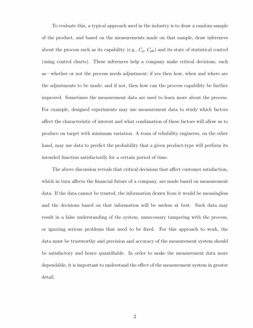
Consider a random sample of ten parts drawn from a production process. The vari-
ation in the true value of the dimension of interest of these parts is known as part-to-part
variation or part variation or process variation (PV). To quantify this variation, these
parts go through a measurement process which adds its own variation known as mea-
surement variation (MV) as mentioned above. The observed variation, which acts as
an input to decision making, is essentially a combination of PV and MV. Figure (1.1)
illustrates how the inherent process variation can be amplified by the measurement sys-
tem. Measurement variation stems from the fact that neither the equipment used for
measurement, nor the appraisers using the equipment are perfect with respect to pre-
cision and accuracy. Ideally, we would like MV to be zero so that process variation
can be estimated without error. But various factors, such as bias and inconsistency of
operators, bias and inconsistency of measuring devices, environmental conditions, and
3

Production System Measurement System Observed Variation
Figure 1.1: Amplification of true process variation
inconsistent sample preparation and measurement processes can introduce measurement
error. As noted by (Barrentine; 1991), measurement error manifests itself in the form of
false conclusions about products with respect to specifications. For example, a product
close to, but within the specification limit, may be classified as defective if the measure-
ment error is large. Similarly, a product out of spec but close to the spec limit may be
classified as non-defective due to measurement error. This increases both producer’s as
well as consumer’s risk. If the data being collected are used for control charting pur-
poses, measurement variation can mask the true process variation and make it difficult
to identify special causes. In a designed experiment, measurement variation can damp
the significance of effects being estimated. Hence it is essential to estimate measurement
error, identify its source and control it within acceptable limits.
1.3 Measurement System Analysis
Measurement System Analysis (MSA) deals with identifying, estimating, analyzing and
controlling various components of measurement error. The Automotive Industry Action
Group (AIAG), a group led by Ford, General Motors and Chrysler has published a refer-
ence manual (AIAG; 1996) for MSA that has become a standard for MSA implementation
across the manufacturing industry. Based on such a study, if the performance of a mea-
4

surement system is found to be unsatisfactory, a company may allocate critical resources
to identify and fix the problem. For example, if the analysis indicates that the high
measurement variation is primarily due to equipment as opposed to appraiser, then the
company may choose to invest in equipment calibration or purchase of new equipment
as opposed to training the appraisers. Hence, it is not only essential that the over-
all measurement error be estimated accurately, but also that it be allocated accurately
among its components—equipment and appraiser. These estimates are based on statisti-
cal properties of multiple measurements obtained from a measurement system operating
under stable conditions (AIAG; 1996). The two primary techniques used to estimate the
components of measurement variation are discussed in the following subsections.
1.3.1 MSA Techniques
Analysis of Variance (ANOVA)
The study is performed in the form of a designed experiment based on a two-way random
effects model. Appraiser and part are treated as random effects. Expected mean squares
and observed mean squares are used to obtain point estimates on desired components.
The primary advantages of using ANOVA are that confidence intervals can be calculated
on these components of variance and the interaction component can be estimated.
Range-Based Estimation
This technique uses average range, adjusted with an appropriate factor (d∗2), to obtain
an unbiased estimate of standard deviation. Despite the advantages of ANOVA, this
method is still widely used in industry primarily due to its simplicity. Data are collected
in a spreadsheet format and a series of simple calculations is required to get the desired
5
estimates. This technique is very effective if the part-by-appraiser interaction component
is believed to be small.
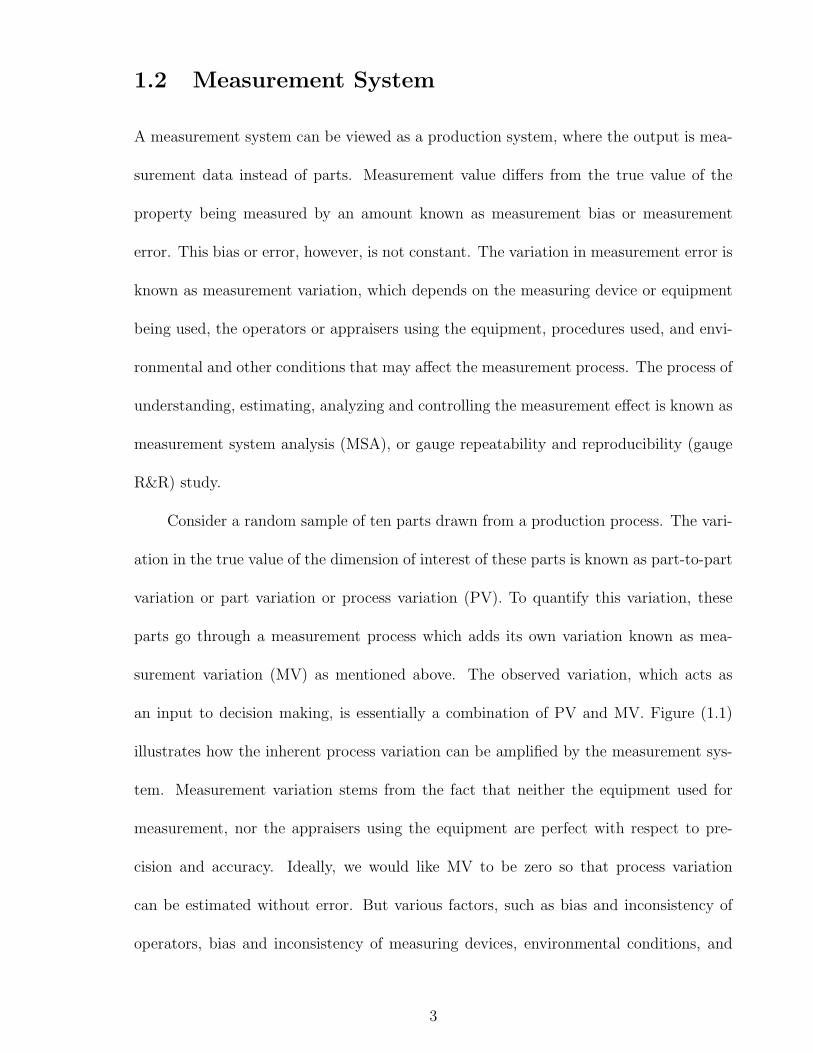
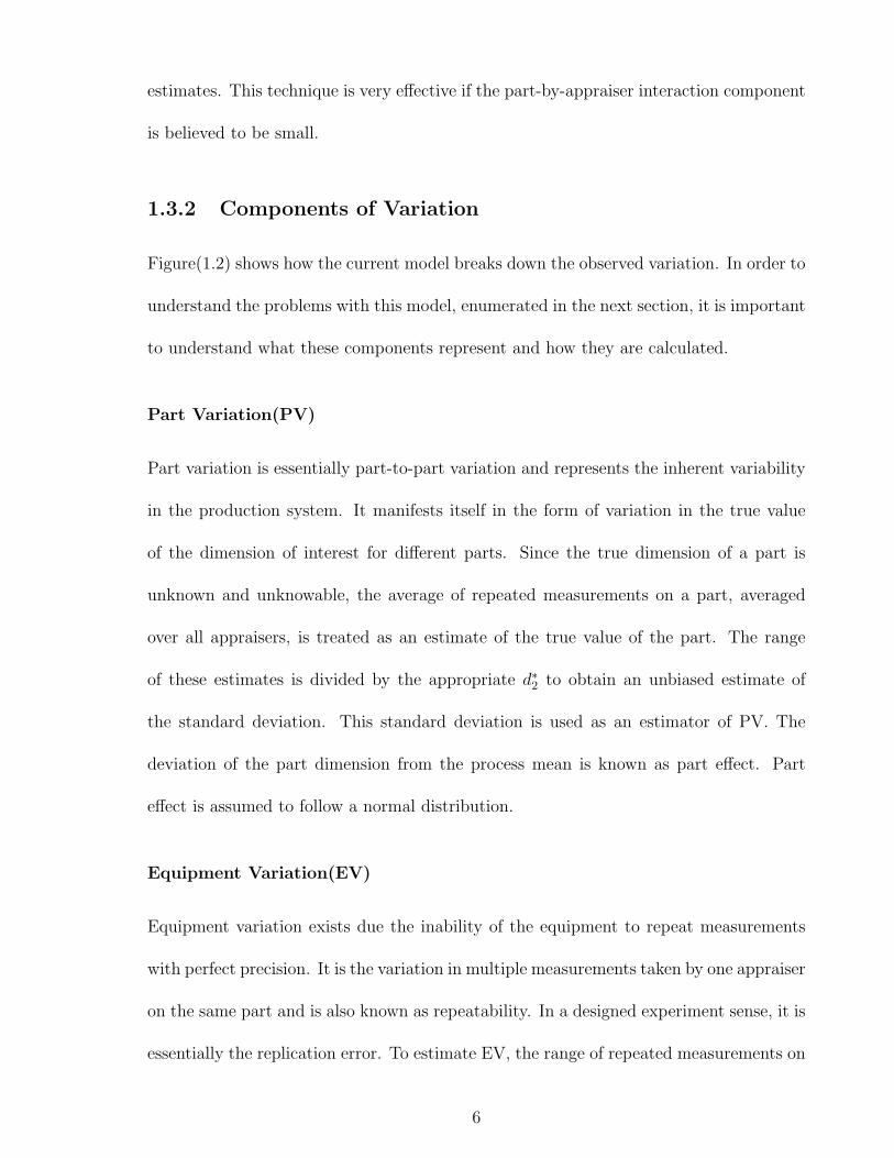
1.3.2 Components of Variation
Figure(1.2) shows how the current model breaks down the observed variation. In order to
understand the problems with this model, enumerated in the next section, it is important
to understand what these components represent and how they are calculated.
Part Variation(PV)
Part variation is essentially part-to-part variation and represents the inherent variability
in the production system. It manifests itself in the form of variation in the true value
of the dimension of interest for different parts. Since the true dimension of a part is
unknown and unknowable, the average of repeated measurements on a part, averaged
over all appraisers, is treated as an estimate of the true value of the part. The range
of these estimates is divided by the appropriate d∗2 to obtain an unbiased estimate of
the standard deviation. This standard deviation is used as an estimator of PV. The
deviation of the part dimension from the process mean is known as part effect. Part
effect is assumed to follow a normal distribution.
Equipment Variation(EV)
Equipment variation exists due the inability of the equipment to repeat measurements
with perfect precision. It is the variation in multiple measurements taken by one appraiser
on the same part and is also known as repeatability. In a designed experiment sense, it is
essentially the replication error. To estimate EV, the range of repeated measurements on
6
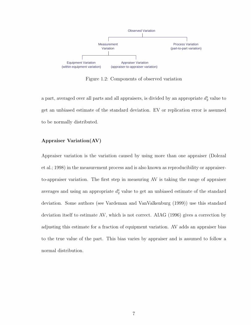
Observed Variation
Measurement Variation
Process Variation (part-to-part variation)
Equipment Variation (within-equipment variation)
Appraiser Variation (appraiser-to-appraiser variation)
Figure 1.2: Components of observed variation
a part, averaged over all parts and all appraisers, is divided by an appropriate d∗2 value to
get an unbiased estimate of the standard deviation. EV or replication error is assumed
to be normally distributed.
Appraiser Variation(AV)
Appraiser variation is the variation caused by using more than one appraiser (Dolezal
et al.; 1998) in the measurement process and is also known as reproducibility or appraiser-
to-appraiser variation. The first step in measuring AV is taking the range of appraiser
averages and using an appropriate d∗2 value to get an unbiased estimate of the standard
deviation. Some authors (see Vardeman and VanValkenburg (1999)) use this standard
deviation itself to estimate AV, which is not correct. AIAG (1996) gives a correction by
adjusting this estimate for a fraction of equipment variation. AV adds an appraiser bias
to the true value of the part. This bias varies by appraiser and is assumed to follow a
normal distribution.
7
1.4 Problems with the Current Model
Some form of MSA has existed, at least for the discrete part manufacturing industry, for
decades. There is still some ambiguity in the terminology and some disagreement among
authors on what the terminology represents. There is also some disparity in definitions
of terms and their mathematical expressions along with the possibility that some com-
ponents of measurement variation have not yet been accounted for. The applicability of
these techniques to continuous process industries presents a whole new challenge.
As mentioned above, AIAG (1996) adjusts the “raw” estimate of AV for a fraction
of equipment variation. The adjusted quantity, also known as reproducibility, still does
not represent true appraiser-to-appraiser variation. Nevertheless, the two terms are used
interchangeably. It is easy to demonstrate a disparity in the definition and the formula
for reproducibility (Vardeman and VanValkenburg; 1999).
Under the current model, replication error is entirely attributed to the equipment.
As will be shown shortly, the replication error may have another component to it besides
equipment variation. This makes the definition of repeatability a little ambiguous. Does
it now represent equipment variation or replication error, as they are not the same any
more? Hence, there may be some disagreement in the definitions of the terms repeata-
bility and reproducibility. As Burdick et al. (2003) noted, such labels do not add value
to answering the questions of interest. Hence, we will refrain from using these terms
throughout this document. The following four subsections summarize the problems in
the current state of MSA that this research will focus on.
8
1.4.1 Within-Appraiser Variation
Within-appraiser variation is the variation due to the inability of an appraiser to repeat
measurements with perfect precision. A closer look at EV above reveals an underlying
assumption that if identically performed measurements on a part are not exactly the
same, then the variation must be due to the imprecision of the equipment. The fact
that appraiser imprecision, if it exists, would also manifest itself in the same way, is
completely ignored. It is equivalent to assuming perfect precision within each appraiser.
In practice, however, it is possible that variation in measurements on the same part
(using the same equipment and appraiser) may be partly due to appraiser imprecision or
within-appraiser variation. It is easy to see that ignoring within-appraiser variation may
produce inflated estimates of EV. Hence, it is possible that a company decides to invest
in re-calibrating or buying new equipment based on high EV estimates, when the real
problem is appraiser imprecision and training appraisers may be a more effective strategy.
The traditional model (AIAG; 1996) does not account for appraiser imprecision or within-
appraiser variation.
1.4.2 Equipment-to-Equipment Variation
Typically only one equipment is used in an MSA study. EV is essentially the within-
equipment variation as indicated in Figure(1.2) above. This restricts the validity of
the inferences drawn to that particular equipment or measuring device. In practice, a
measurement system may consist of multiple equipment and a significant portion of the
observed variation may be due to the fact these equipment are not consistent with each
other. In other words, there may be a bias associated with the equipment. A company
9
may be interested in knowing variation among equipments and the current approach
does not allow for that. Using multiple equipments in the study will allow us to estimate
among-equipment or equipment-to-equipment variation and may produce more realistic
estimates of the true process variation. It should be noted that each equipment being used
may have a different within-equipment variation. The model should explicitly account
for that.
1.4.3 Adjusting the Estimate for Part Variation
The method for estimating PV was described in the previous section. It is easy to show
that this technique estimates is not just PV, but a sum of PV, a fraction of EV and
a fraction of part-by-appraiser interaction. The current technique clearly overestimates
PV. The magnitude of EV and the interaction component and the number of replications
and appraisers used in the study determines how significant this overestimation would
be.
1.4.4 Applicability to Chemical and Process Industries
MSA in its current form uses statistical properties of multiple measurements on the same
part to estimate the various components of measurement variation. In chemical and pro-
cess industries most tests are destructive in nature. For example, measuring the moisture
content of a sample of a chemical compound will require it to go through a test that will
end up destroying the sample. This makes is impossible to take multiple measurements on
the same sample. Hence, the traditional approach of estimating components of variance
cannot be used. There is a very high demand in this industry for a statistically sound
approach that will identify and accurately estimate various components of measurement
10
variation.
1.5 Measurement System Acceptability Criteria
Once measurement variation and its variance components have been estimated, the goal
is to reduce measurement variation to acceptable levels, if it is not already. Hence, it is
important to determine how much measurement variation should be considered accept-
able and what criteria should be used to make that decision. A wide range of metrics can
be found in the literature to evaluate the measurement system capability. For example,
precision-to-tolerance ratio, percent total variation, percent process variation, intraclass
correlation coefficient, discrimination ratio, number of distinct data categories (or clas-
sification ratio) and probable error. All these metrics come with certain recommended
values that suggest the acceptability of the measurement system. The question that
remains to be answered is whether these metrics, if used in the recommended manner,
produce consistent outcomes with respect to the acceptability of the measurement sys-
tem under study. In other words, is it possible that some of these metrics conclude that
a measurement system is acceptable while others conclude otherwise. If so, then under
what conditions does this discrepancy occur and which metrics, if any, are relatively
robust to variations in these conditions.
11
1.6 Objectives
General Objective
Identify any components of variation ignored in the traditional MSA, improve upon the
existing estimates and expand the applicability of MSA to industries other than discrete
part manufacturing.
Specific Objectives
1. Account for within-appraiser variation.
• Develop a mathematical model consistent with the concept of within-appraiser
variation.
• Derive lower bound on within-appraiser variation.
• Use the lower bound to adjust the EV estimate appropriately.
• Show that the estimates of other components of variance do not change as a
result of this development.
• Use simulation to demonstrate the effectiveness of the bounds.
2. Enhance the current MSA approach so that inferences drawn will be applicable to
all equipment in the measurement system.
• Develop guidelines for selecting and using multiple equipment and collecting
data.
• Derive estimates for equipment-to-equipment variation.
• Appropriately adjust estimates of other components of variance that may have
changed as a result of this development.
12
• Verify the estimates using simulation.
3. Derive mathematically correct expression for PV and demonstrate its superior ac-
curacy over the traditional estimate.
4. Evaluate various measurement system acceptability criteria
• Conduct a simulated experiment by varying the sigma-capability of a process
and draw conclusions about relative merits and robustness of the metrics.
5. Develop a methodology similar to MSA for application in chemical and process
industries.
• Develop guidelines for determining sample sizes, sample selection and data
collection.
• Identify any sources of variation in addition to the conventional sources for
the discrete part case.
• Develop a mathematical base for estimating the contribution of each of these
sources.
• Use simulation to verify the estimates.
13
Chapter 2
Literature Review
2.1 Nomenclature and Notation
Measurement system analysis (MSA), also known as gauge capability analysis or gauge
repeatability and reproducibility analysis is an effort to understand, identify, quantify
and control the sources of measurement variation (Burdick et al.; 2003; Potter; 1990;
Montgomery and Runger; 1994a; Dolezal et al.; 1998). There is a consensus among au-
thors that variation in identically performed measurements on the same part is primarily
due to measurement error. One of the primary objectives of MSA, though, is the isola-
tion of the sources of variability in the measurement system (Burdick et al.; 2003). It
is in this stage that a severe lack of standardization in nomenclature and notation is
obvious (John; 1994). Authors disagree on everything from trivial things like spellings of
terms (gauge or gage), kind of alphabet used to represent the underlying model (greek
or roman, capital or small) to more serious issues like the meaning of repeatability and
reproducibility and what they represent.
In order to understand these differences, it is important to introduce some notation
and define the basic underlying model. The notation used here will be consistent with
AIAG (1996) as it is the most widely used reference in the industry for MSA implemen-
tation. MSA is typically conducted in the form of a two-factor experiment based on
14

random effects model (Vardeman and VanValkenburg; 1999; Dolezal et al.; 1998). This
means that a certain number of parts are randomly selected and are measured multiple
times by randomly selected appraisers (or operators). The underlying model is given by
yijm = µ + αi + βj + (αβ)ij + εijm (2.1)
where i = 1, ..., n j = 1, ..., k m = 1, ..., r
The subscripts i, j, and m represent part, appraiser and measurement (or replica-
tion), respectively. The term yijm represents the mth measurement by the jth appraiser
on the ith part and µ is an unknown constant. The terms αi, the part effect; βj, the
appraiser effect; αβij, the part-by-appraiser interaction; and εijm, the replication error
are independently and normally distributed with mean zero and variance σ2p, σ
2a, σ
2pa and
σ2, respectively.
There is a general agreement among authors that the variance of identically per-
formed measurements on the same part, or the replication error variance (σ2) is the
repeatability of the measurement system. Reproducibility, however, has been defined
in multiple ways. AIAG (1996) defines reproducibility as variation among appraisers
or simply appraiser variation (AV) and use σ2a as an estimate of AV or reproducibility.
Mitchell et al. (1997) also use σ2a to estimate reproducibility. Wheeler (1992) criticizes re-
producibility as it tells only that the appraiser-to-appraiser differences are significant but
gives no information about which appraiser(s) is the problem. He states that reproducibil-
ity is useless when applied to a measurement process used in-house. Montgomery and
Runger (1994a) prefer to use σ2a +σ2
pa to estimate reproducibility, but they do not specif-
ically call it appraiser-to-appraiser variation. They reason that since part and appraiser
are the only two factors in the study and the interaction effect is essentially a measure-
15
ment error, it should be included in the reproducibility. Vardeman and VanValkenburg
(1999) also use σ2a+σ2
pa to estimate reproducibility and specifically call it variation among
operators. Their reasoning is a little more mathematical. They suggest that for any one
part (i = 1), the model (2.1) reduces to y1jm = µ+α1+βj +αβ1j +ε1jm. If γj = βj +αβ1j,
then the variance of γj, σ2a +σ2
pa, clearly represents variation among appraisers. Unfortu-
nately, the same reasoning can be used to include σ2pa in part or process variation (PV).
For instance, the model in Eq(2.1) reduces to yi1m = µ + αi + β1 + αβi1 + εi1m for any
one appraiser (j = 1). Now, if γi = αi + αβi1, then the variance of γi, σ2p + σ2
pa, clearly
represents part-to-part variation. Vardeman and VanValkenburg (1999) recognize this
anomaly and use it to dispute σ2p as an estimate of PV. They argue that the interaction
variance should be a part of both PV and AV.
All this discrepancy and confusion seems to originate from the obvious compulsion to
label all the variance components. The term σ2pa represents the variance of the interaction
effect and should be recognized as such. Any attempt to arbitrarily include it with AV or
PV will be misleading. The terms σ2p and σ2
a are the only true estimates of part-to-part
(PV) and appraiser-to-appraiser (AV) variation, respectively. It is acceptable, however,
to label σ2a +σ2
pa as reproducibility as long as it is recognized that reproducibility and AV
will not be the same in that case. As Burdick et al. (2003) have pointed out, such labels
do not add value to our understanding of the system and hence we will purposefully
refrain from using them.
16
2.2 Planning the Study
Literature addressing issues related to measurement error can be traced back to the
1940s (Grubbs; 1948). Early research was primarily focused on avoiding the potential
loss due to measurement error. Eagle (1954) suggests tightening of specifications for
testing purposes to minimize the risk of committing β-error (accepting a non-conforming
part). This, however, increases the risk of committing α-error (rejecting conforming
parts). Besides, this is a reactive approach and does not help much in estimating and
reducing measurement error.
Most techniques used today are proactive and concentrate on estimating and re-
ducing the measurement error. Eagle (1954) states that determining measurement error
requires repeated measures using one device and multiple operators or multiple devices
and one operator. The most widely used form of MSA today employs one device and
multiple operators. There is no reason why multiple devices and multiple operators can-
not be used. Montgomery and Runger (1994b) give a mathematical model for such a
case. Whenever an additional factor is added to the experiment, a decision must be made
as to whether the sample will be selected randomly or not. If all factors are random,
the underlying model is called a random-effects model; if all factors are fixed, it is called
a fixed-effects model; and if some factors are random and others are fixed, it is called
a mixed model. This becomes especially relevant when using the ANOVA technique
described later in this section. It is important to note that if a factor is treated as ran-
dom, the inferences about its effect are applicable to the entire population from which
the sample was drawn. On the other hand, if a factor is treated as fixed, the inferences
about its effect are restricted to the specific levels employed in the experiment. Hence,
17
the decision to treat a factor as fixed or random must be made judiciously, depending
on the desired outcome. Hahn and Nelson (1970), for example, suggest using a mixed
model with a single appraiser, randomly selected parts, and fixed measuring devices.
Dolezal et al. (1998) show the analysis of a mixed model case with fixed operators. It is
interesting to see that whereas the confidence intervals (CI) of random effects are based
on the Chi-square distribution, the CI of fixed effects in a mixed model situation are
based on a non-central Chi-square distribution with a specific non-centrality parameter.
Montgomery and Runger (1994a) recommend that even if the number of operators is
very small and can be a fixed factor, it should be treated as a random draw from the
potential population of operators.
Montgomery and Runger (1994a) recommend using a larger number of parts with
fewer measurements on each. They list multiple advantages of doing this—(i) a gauge
may be more stable near the center of the operating range than towards the extremes
and using many parts increases the chances of detecting any such non-linearity; (ii) if the
measurement variance depends on the mean measurement, this trend can be detected;
and (iii) it is difficult to get complete replication of measurement and hence, too many
measurements on a part increase the chance of introducing other factors of variability.
Wheeler (1991) recommends only two replications for the same reason. Montgomery and
Runger (1994a) also caution against placing too much emphasis on keeping conditions
“identical” during replications. Since such care is usually not taken during routine mea-
surements, this may cause the underestimation of measurement error. They recommend
that if linearity is an issue, then parts must be chosen over the entire operating range
of the instrument, even beyond the specification. In such a case using a random sample
may not be the best choice.
18
Depending on the situation, there may be many factors that affect the measure-
ment process. Montgomery and Runger (1994a) recommend using 25% or less of total
resources in the initial study for identifying important factors through fractional factorial
or screening designs.
2.3 Analyzing the Data
The two most commonly used techniques to estimate measurement variance components,
as mentioned above, are the range-based method and ANOVA. These are discussed in
greater detail in the following sections.
2.3.1 Range-Based Estimation
Patnaik (1949) notes that the distribution of the range in normal samples is independent
of the population mean, but depends on the sample size and population standard devia-
tion. He gives the mathematical basis for the factor d2, which is based on sample size and
is used to estimate the standard deviation from the sample range. AIAG (1996) suggest
that the value of d2 should also depend on the number of samples used. They introduce a
new factor d∗2 that varies with both number of samples and the sample size, and converges
to d2 as number of samples become large (fifteen or more). Wheeler (1992) considers d∗2
to be an unnecessary complication as the uncertainty in the range will usually be greater
than the difference between d2 and d∗2. It has, however, become a common practice in
MSA to use d∗2 and we will continue with the practice. Vardeman and VanValkenburg
(1999) provide a statistical basis for the range-based approach
Most authors in the recent literature discourage the use of range-based approach
19
(Montgomery and Runger; 1994b; Burdick et al.; 2003; Vardeman and VanValkenburg;
1999; John; 1994). The main criticism of this approach is that it does not allow for the
estimation of the interaction variance component, does not allow for the construction of
confidence intervals on the variance components and gives a downwardly biased estimate
of reproducibility. Patnaik (1949) himself notes that range furnishes a less efficient esti-
mate of standard deviation. John (1994) use an example from Wheeler (1992) to show
that the estimates obtained using this approach vary significantly from the ANOVA-based
estimates. John (1994) indicates that using ranges is inappropriate for the semiconductor
industry. With the modern-day computing power, most practitioners are moving away
from this approach toward the ANOVA-based approach. However, there are still a lot of
companies that use this approach and hence it cannot be ignored.
There is a general consensus among authors in the way the repeatability (or replica-
tion error) standard deviation is calculated. The range of multiple measurements taken
by an appraiser on a given part is calculated. This range is averaged over all parts
and appraisers, divided by the appropriate d∗2 to obtain an unbiased estimate of standard
deviation that represents repeatability. For calculating reproducibility, multiple measure-
ments taken by an appraiser are averaged over all parts. The range of these appraiser
averages is divided by d∗2 to estimate reproducibility standard deviation. It is easy to
show that this estimate represents σ2a + 1
nσ2
pa + 1nr
σ2. Vardeman and VanValkenburg
(1999) note that some authors like Montgomery (1996) and Kolarik (1995) use this to
estimate AV. This will obviously result in overestimate of AV. Vardeman and VanValken-
burg (1999) criticize AIAG for adjusting this estimate for the fraction of σ2 but not for
the fraction of interaction variance, σ2pa. AIAG (1996), however, clearly indicate that the
range-based approach should be used only if the additive model is deemed appropriate,
20
i.e., the interaction effect can be neglected. Montgomery and Runger (1994a) introduce
an alternative way of calculating reproducibility. The average of replicate measurements
by an appraiser on each part is calculated. The range of these averages is obtained for
each part. The average of these ranges is used to estimate reproducibility. The variance
calculated in this manner represents σ2a+σ2
pa+ 1rσ2. Vardeman and VanValkenburg (1999)
also use this estimate but emphasize that it must be adjusted for a fraction of σ2.
2.3.2 Analysis of Variance (ANOVA)
Analysis of variance is a technique used to partition the total sum of squares into a portion
due to regression and a portion due to error (Walpole and Myers; 1985). The sum of
squares due to regression is further partitioned into various factors and interactions. The
error mean square is pure replication error, or repeatability. Other variance components
(VC) are not directly readable from the ANOVA table. Their values need to be calculated
using expected mean square (EMS) values. Most statistical software can provide EMS
values for all factors and interactions based on the assumptions of the underlying model.
For guidelines on deriving EMS the reader is referred to Kuehl (2000) or Montgomery
(2001). Even though normality of effects is a basic assumption of ANOVA, Montgomery
and Runger (1994b) state that normality is not essential to use EMS for obtaining VC
estimates. However, they note, if the assumption is met, it is easy to construct confidence
intervals on the VCs.
Most authors agree that the estimates based on ANOVA are more accurate and
allow for the construction of confidence intervals and estimation of interaction effects as
stated above. One of the disadvantages of using ANOVA, however, is that the estimates
of VCs may turn out to be negative (Montgomery and Runger; 1994b). Kuehl (2000)
21
suggests various remedies for this problem. One remedy is to assume the VC to be zero;
but that may produce biased estimates of other VCs as noted by Montgomery and Runger
(1994b). They suggest using a modified ANOVA, which is nothing but redoing ANOVA
with the insignificant term (usually the interaction term) removed. This allocates the
degrees of freedom for that term to error. Another solution is to use other methods of
estimating VCs (Kuehl; 2000; Montgomery and Runger; 1994b).
2.3.3 Other Techniques
Wheeler (1992) very strongly recommends using graphical techniques in place of the
traditional analysis. He plots an X-chart of the operator averages of three operators
and suggests that an out of control condition indicates a significant operator difference.
With control limits based on just three points, however, it may inappropriate to place
too much confidence in the outcome.
Montgomery and Runger (1994b) suggest methods such as maximum likelihood es-
timates (MLE) or MINQUE estimates. MLEs maximize the likelihood function of the
sample such that each VC is required to be non-negative. MINQUE produces estimates
that are best quadratic unbiased and are guaranteed to be non-negative. Both these
procedures are iterative in nature. These estimates, as illustrated by Montgomery and
Runger (1994b), give a covariance matrix of all VCs. The variance of each VC, obtained
from the diagonal elements of this matrix, along with the assumption of normality al-
lows the construction of confidence intervals using z-values. These intervals are easy to
construct and are usually narrower than those obtained from ANOVA. A non-iterative
version of MINQUE also exists, but it is not guaranteed to produce non-negative esti-
mates (Montgomery and Runger; 1994b). Both MLE and MINQUE require specialized
22
software and give estimates close to those obtained by using modified ANOVA. Hence
ANOVA has become the technique of choice.
2.4 Some Problems With MSA
Recall that the objective of this research is to address the issue of within-appraiser
variation and among-equipment variation, provide correct estimate for PV and adapt
MSA to address the needs of chemical and process industries. This section will address
any previous work in these areas.
2.4.1 Within-Appraiser Variation
No previous research has explicitly acknowledged the existence of within-appraiser vari-
ation or addressed the issue otherwise. Some relevant work will be discussed here.
Burdick et al. (2003) note that the variance of measurements may not remain con-
stant in all cases. One reason given, if this variance varies over time, is “operator fatigue”.
Fatigue results in the appraiser’s inability to keep the bias constant over time. This vari-
ation in appraiser-bias is essentially within-appraiser variation. The time-dependence in
the case of operator fatigue makes it easy to spot such variation by plotting residuals
against time. If, however, the variation is due to inadequate training or other human
factors, there may not be a covariate such as time.
Montgomery and Runger (1994a) mention that an out of control condition on the
R chart plotting ranges of measurements would indicate that the appraiser is having
difficulty using the equipment. If indeed this is the case, it is possible to get an R chart
that is in a state of statistical control but has very wide control limits. This would
23
happen if the appraiser inconsistency, or the within-appraiser variation, is randomly
scattered over all measurements. Wide control limits on an R chart would lead to high
estimates of equipment variation since the variance of measurements, or replication error,
is typically attributed to equipment.
To summarize the above discussion, some authors have shown that within-appraiser
variation can be detected either through residual plots if a covariate is present or through
control charts if appraiser inconsistencies are rare and sporadic. If, however, the appraiser
is regularly inconsistent in the use of measuring devices, these tools may not detect within-
appraiser variation. In such a case, a plot of measurement ranges sorted by appraiser
may be helpful. For example, if the average range of an appraiser shows a significant
shift, high variation can be assumed within that appraiser. The absence of shift, however,
should not be confused with the absence of appraiser inconsistency as it will only indicate
that appraiser inconsistency does not vary significantly from appraiser to appraiser.
2.4.2 Using Multiple Equipment
As noted earlier, if routine implementation of the measurement system involves multi-
ple equipment, there may be a significant equipment-to-equipment variance component
involved. Montgomery and Runger (1994b) proposes a model that adds equipment as
another factor to the experiment. However, there has been no effort to estimate vari-
ance components under this scenario. Despite is potential usefulness, this model is rarely
implemented in practice.
24
2.4.3 Correcting the Estimate of PV
The estimate of PV provided by AIAG has not been challenged by any researcher. Yet,
there is a small but definite error in the formula, as will be shown in the next chapter.
2.4.4 MSA for Chemical and Process Industries
Within MSA, the research effort devoted to chemical and process industries where test-
ing is destructive, is an order of magnitude less than that devoted to the discrete part
manufacturing case.
Some authors that have addressed the issue, focus on minimizing the within-sample
variation and treating measurements on different subsamples as different measurements
on the same sample (Spiers; 1989; Ackermann; 1993).
Spiers (1989) uses an example, measuring tensile strength of tin, to illustrate this.
They cut thirty samples from a single sheet of tin and randomly assigned ten samples to
each of three appraisers. Each sample was then cut into three subsamples. The tensile
strength measurement on each of these subsamples was treated as multiple measurement
on the sample. The differences were considered negligible among subsamples due to
adjacency.
Ackermann (1993) recognizes that choosing samples for such a study is the most
critical step and that care should be taken to minimize lot-to-lot, within lot and within
sample variation. She further states that high material variation can mask out the
appraiser-to-appraiser variation. Even though this is true, if all material variation is
minimized the results of such a study will be valid only for that narrow range of val-
ues. Any non-linearity in the measurement system will never be discovered under such
25

circumstances. For example, if the objective is to measure the moisture content of a
chemical compound and all material is chosen so that the moisture content is very close
to 0.5%, then we will never know how the measurement system behaves if the moisture
content in the sample rises to, say, 1%. This is the reason why authors like Montgomery
and Runger (1994a) have emphasized the fact that parts should be chosen over the entire
range of values that the measurement system can measure. This allows for the assess-
ment of linearity in the measurement system. To minimize the masking out of AV, as
alluded to by Ackermann (1993), the first sample assigned to each appraiser should be
near identical, so should the second sample and so on.
Ackermann (1993) notes that merely minimizing material variation is not enough;
the differences, must be accounted for. Yet, in this paper, measurements by an appraiser
on multiple subsamples are treated as multiple measurements on the same sample and
any differences among these subsamples are ignored. The work presented in this paper
is based on the work of Spiers (1989), who also ignores these differences. The work of
Spiers (1989) and Ackermann (1993) is relevant to this discussion in that they address
the issue of destructive testing. However, the applications presented are not from the
CPI, where sampling issues can be much more complex. It may be reasonable to ignore
differences among subsamples in some of these cases, for example, the tensile strength
measurement of a tin sheet.
ASQ Chemical and Process Industries Division (2001) throws some light on sampling
issues in the CPI. They recommend repetitive sampling of incoming material to establish
homogeneity, but acknowledge that when a specimen is destroyed, there is an additional
variability from specimen to specimen, however small it has been made. Besides, for
a sample to be truly representative of the population, it must be random. For gases
26
and liquids, sampling ports may limit any consideration for randomness. For example,
accessibility restricts true randomness for materials in storage silos, railcars, etc. (ASQ
Chemical and Process Industries Division; 2001). Besides, randomness can be especially
difficult to achieve if sampling is done on a time-frequency basis. The ASQ Chemical and
Process Industries Division (2001) states that the element of time and its ramifications
on sampling is one of the major differences between the CPI and the discrete part manu-
facturing industry. They further state that in CPI, production processes often drift over
time and data are autocorrelated; data are based on individual measurements and many
production processes are not in a state of control; specifications are often not statistically
based on production processes and measurement system knowledge.
Wheeler (1991) recommends using a range-chart by plotting measurement ranges.
An out of control condition on such a chart can indicate that either the measurement
system is out of control or that the samples measured were not homogenous. Such a chart
will be useful only if a reasonable assurance of sample homogeneity can be achieved. ASQ
Chemical and Process Industries Division (2001) suggest plotting two types of control
charts — a production process control (PPC) chart and a measurement system control
(MSC) chart. The former is a regular control chart created by measuring material actu-
ally being produced. The latter, however, is created using control material (CM) local to
the particular site. The objective of the former is to determine whether the production
process is in control, while that of the latter is to ensure that the measurement system is
accurate and precise enough for the PPC chart to be trusted. However, if the sampling
frequency is not high enough, the MSC chart may fail to serve its intended purpose. For
example, if the average run length (ARL) of the PPC chart for a shift of, say, x units is
less than the ARL of the MSC chart, and if a shift of x units occurs in the measurement
27
system, then the PPC chart will detect it before the MSC chart and unnecessary tamper-
ing with the process may occur (ASQ Chemical and Process Industries Division; 2001).
To ensure that changes in the measurement system are detected by the MSC chart before
the PPC chart, the ASQ Chemical and Process Industries Division (2001) recommends
that the ARLMSC = 12ARLPPC .
Mitchell et al. (1997) have come up with a very interesting approach to address
the issue of using MSA for destructive testing. Bergeret et al. (2001) use these results
in three different applications. The applications have been chosen such that testing is
not destructive. Then this technique is used pretending that the testing is destructive.
The results are compared with regular MSA study to assess the effectiveness of the
technique. In this technique, the experiment is performed in two stages. In stage one
only one operator is used, who divides each sample into subsamples and measures them.
The equipment variation is assumed to be confounded with subsample variation. In the
second stage multiple operators measure each sample only once. The equipment variation,
in this stage, is assumed to be confounded with sample variation. A simple manipulation
of expected mean squares from the two stages, yields the equipment variation.
2.5 Evaluating Measurement System Acceptability
Criteria
This section identifies various metrics used to assess measurement system acceptabil-
ity and the criteria associated with them. Some such metrics being discussed here are
summarized in Table (2.1)
28
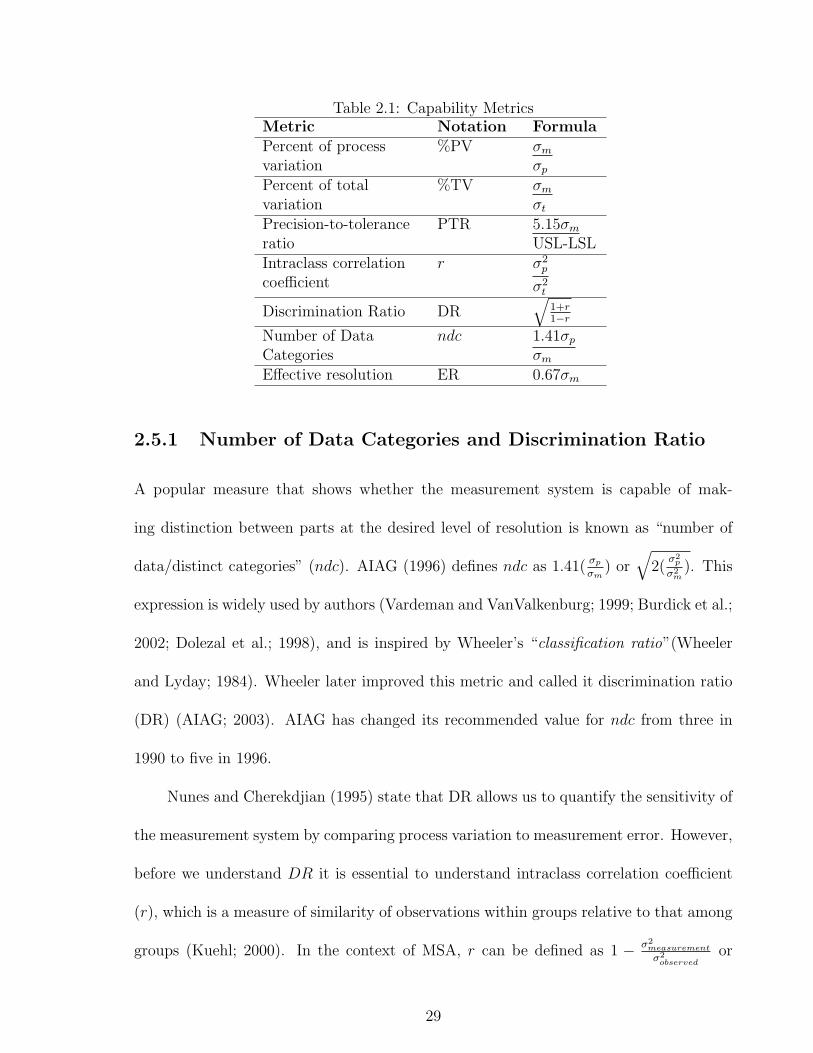
Table 2.1: Capability MetricsMetric Notation FormulaPercent of processvariation
%PV σm
σp
Percent of totalvariation
%TV σm
σt
Precision-to-toleranceratio
PTR 5.15σm
USL-LSLIntraclass correlationcoefficient
r σ2p
σ2t
Discrimination Ratio DR√
1+r1−r
Number of DataCategories
ndc 1.41σp
σm
Effective resolution ER 0.67σm
2.5.1 Number of Data Categories and Discrimination Ratio
A popular measure that shows whether the measurement system is capable of mak-
ing distinction between parts at the desired level of resolution is known as “number of
data/distinct categories” (ndc). AIAG (1996) defines ndc as 1.41( σp
σm) or
√2(
σ2p
σ2m
). This
expression is widely used by authors (Vardeman and VanValkenburg; 1999; Burdick et al.;
2002; Dolezal et al.; 1998), and is inspired by Wheeler’s “classification ratio”(Wheeler
and Lyday; 1984). Wheeler later improved this metric and called it discrimination ratio
(DR) (AIAG; 2003). AIAG has changed its recommended value for ndc from three in
1990 to five in 1996.
Nunes and Cherekdjian (1995) state that DR allows us to quantify the sensitivity of
the measurement system by comparing process variation to measurement error. However,
before we understand DR it is essential to understand intraclass correlation coefficient
(r), which is a measure of similarity of observations within groups relative to that among
groups (Kuehl; 2000). In the context of MSA, r can be defined as 1 − σ2measurement
σ2observed
or
29
1− σ2m
σ2o
and DR has been defined by Wheeler (1992) as
DR =
√1 + r
1− r(2.2)
=
√2σ2
o
σ2m
− 1
Wheeler (1991) recommends that DR should be five or more for the measurement system
to be useful. Dolezal et al. (1998) state that the measurement process is adequate if the
DR is greater than or equal to three. Burdick et al. (2003) define DR as 1+r1−r
(without
the square-root) which is incorrect.
Wheeler (1991) states that DR defines the number of product categories that the
measurement will support. AIAG (1996) define ndc as the number of distinct levels of
product dimensions (or categories) that can be reliably obtained from the data. Both
these quantities are not only similar in concept but turn out to be very similar in value.
2.5.2 Precision-to-Tolerance Ratio (PTR)
Another measure of interest is precision-to-tolerance ratio (PTR) given by
PTR =5.15σm
USL− LSL(2.3)
PTR is considered to be the fraction of the tolerance consumed by the measurement
system (Montgomery and Runger; 1994a; AIAG; 1996; Burdick et al.; 2003; Mitchell
et al.; 1997). Wheeler (1992), however, states that whenever two quantities are compared
by a ratio there is an implicit assumption that the numerator can be added to some other
quantity to yield the denominator . He presents a convincing argument that measurement
error and tolerance are not additive since standard deviations are not additive, and
hence the former does not ”consume” the latter and it is misleading to use such ratios.
30
Moreover, this ratio provides no information about the capability of a measurement
system to detect product variation. For example, Spiers (1989) considers the micrometer
under investigation to be capable because it consumes only 18% of the tolerance. The
truth is, it tells us nothing about the capability of the instrument to distinguish among
product categories. Wheeler (1992) states that a measurement system with high PTR
(undesirable) can be capable of detecting product variation if PV is large and vice versa if
PV is low. Some authors like Montgomery and Runger (1994a) and Burdick et al. (2003)
strongly advocate the use of this ratio and state that PTR of 10% or less indicates an
adequate measurement system. Montgomery and Runger (1994a), however, acknowledge
that PTR can be minimized to any desired value by artificially inflating the specifications.
Morchower (1999) indicates a PTR of 5% or less is preferable.
Sometimes a multiplier of 6 instead of 5.15 may be used in Eq(2.3) (Burdick et al.;
2003). Mitchell et al. (1997) also uses the reciprocal of this ratio as measurement capa-
bility index (Cp).
2.5.3 Other measures
AIAG (1996) also use “percent of Total Variation (%TV = 100MV/TV )”, where MV
and TV represent measurement variation and total variation respectively, as a measure of
measurement system capability. Wheeler (1992) states that even though this measure is
meaningful in terms of indicating the usefulness of the measurement system, it still suffers
from the other problem stated above–total variation and measurement variation are also
not additive and hence should not be compared using a ratio. For example, a %MV of
30% does not indicate, contrary to popular belief that measurement variation is 30% of
total variation. Taking the ratio of variances instead of standard deviations may eliminate
31
Wheeler’s concern with this ratio and may meaningfully represent the portion of observed
variation that is due to measurement. Another performance measure, which is similar to
%PV and is often used, is “percent of Process Variation (%PV = 100MV/PV )”, where
PV represents process or part variation. Montgomery and Runger (1994a) consider these
two to be more useful than PTR.
Wheeler (1991) gives another measure called “effective resolution” which is the max-
imum of two quantities—probable error and measurement unit, where probable error is
defined as 0.67σmeasurement.
32
Chapter 3
Theoretical Background
Chapter Overview
The model presented by AIAG, which is the basis for most MSA studies, will be referred to
as the “current model” or the “traditional model”. A mathematical basis for the estimates
of equipment variation (EV), appraiser variation (AV) and part variation (PV) using both
the range-based method and ANOVA will be developed. In an attempt to resolve the
issue of within-appraiser variation, a new model will be proposed. A mathematical basis
will be developed for within-appraiser variation and any effect of the changes made to the
traditional model on estimates of EV and AV, will be investigated. To allow for multiple
measuring equipment in the study, an enhanced version of the traditional model will be
presented, and new estimates with respect to additional equipment will be derived. A
corrected formula, based on the traditional model, for PV and discrimination ratio will
be derived. Procedures for the verification of all enhancements and alterations to the
traditional model will be outlined.
3.1 Current Model
The linear model underlying the traditional MSA techniques is given in Eq(2.1) as yijm =
µ + αi + βj + (αβ)ij + εijm. The meaning of these symbols is described in Section 2.1.
33
Consider a study conducted with one measuring device, k randomly selected ap-
praisers and n randomly selected parts. Each appraiser measures each part r times. The
estimates of various variance components will be derived for this scenario.
3.1.1 Range Based Estimates of Variance Components
Using average range to estimate standard deviation has been an old tradition in the field
of quality. A brief explanation of the statistical theory behind this is provided here.
Vardeman and VanValkenburg (1999) is the primary source of this explanation. Suppose
that x1, . . . , xn are IID normal (µ, σ2) variables, then their range is given by
R = max xi −min xi
= σ
(max
(xi − µ
σ
)−min
(xi − µ
σ
))
This implies that R has the distribution of a σ multiple of the range of n standard normal
variables. Now, consider n standard normal variables, z1, . . . , zn. Let their range be given
by W = max zi −min zi and the expected value of W be given by E[W ] = d2(n). If the
average of multiple such ranges is given by R, then Rd2(n)
= σ. Then, clearly, the expected
value of R is given by E[R] = σd2(n) and E[
Rd2(n)
]= σ. For details on the distribution of
range of standard normal variables, W , and the calculation of d2(n) values, see Patnaik
(1949). Tabulated values of d2(n) for reasonable values of n can be found in most quality
control books. AIAG recommends using d∗2(n) instead, which takes into account the
number of ranges that the average is based on. These values can be found in AIAG
(1996) for subgroup sizes of up to fifteen and number of ranges up to fifteen and in AIAG
(2003) for subgroup sizes and number of ranges up to 20. For more details and other
values of d∗2(n), the reader is referred to Duncan (1974) and Elam (2001).
34
It would be advantageous, at this point, to introduce some notation. As noted
earlier, yijm represents the mth measurement by the jth appraiser on the ith part. The
average of r measurements taken by the jth appraiser on the ith part is given by yij. =
1r
∑m yijm = µ + αi + βj + αβij + εij.. The bar on the statistic indicates that it is an
average and the subscript over which the average is taken is replaced by a dot. Similarly,
the range of r measurements taken by jth appraiser on the ith part is given by Rijm =
maxm yijm − minm yijm = yijm′′ − yijm′ where m′′ and m′ represent the largest and the
smallest measurement for a given i, j. The subscript on R with an underscore is the one
over which the range has been taken. The average of these ranges over all parts for the jth
appraiser will be given by R.jm = 1n
∑ni=1(maxm yijm−minm yijm) = 1
n
∑ni=1(yijm′′−yijm′).
Equipment Variation
Using the linear model given in Eq(2.1), the range of multiple measurements by the jth
appraiser on the ith part can be represented as Rijm = yijm′′ − yijm′ = εijm′′ − εijm′ where
m′′ and m′ represent the largest and the smallest measurement for a given i, j. Since
εijm represents replication error, and is normally distributed with mean 0 and variance
σ2, we get(
E
[Rijm
d2(r)
])2
= σ2 (3.1)
Using R..m as an estimate of E[Rijm],R..m
d2(r)= σ can be used as an estimate for equipment
variation where
R..m =1
nk
k∑j=1
n∑i=1
(yijm′′ − yijm′) (3.2)
35
Appraiser Variation
The average of all measurements on all parts made by the jth appraiser can be expressed
as
1
nr
n∑i=1
r∑m=1
yijm = y.j. = µ + α. + βj + αβ.j + ε.j. (3.3)
The range of these averages for all appraisers can be expressed as R.j. = (βj′′−βj′)+
(αβ.j′′ − αβ.j′) + (ε.j′′. − ε.j′.) where j′′ and j′ represent appraisers with the largest and
the smallest measurement averages respectively. Since βj, αβij, and εijm are normally
distributed with mean 0 and variance σ2a, σ
2pa, and σ2 respectively, we obtain
(E
[R.j.
d∗2(k)
])2
= σ2a +
σ2pa
n+
σ2
nr(3.4)
Since, only one such range is obtainable for a given experiment, E[R.j.] = R.j. and
R.j.
d∗2(k)=
√σ2
a +σ2
pa
n+
σ2
nr(3.5)
The quantity of interest here, is σ2a, the appraiser variation or appraiser-to-appraiser
variation. As mentioned earlier, some authors like Montgomery (1996) and Kolarik (1995)
use the entire expression in Eq(3.4) to estimate AV. A slightly better estimate is given
by AIAG by correcting for σ2
nr, using EV as an estimate of σ. They recommend using the
range-based approach only if the interaction can be ignored and hence do not adjust this
estimate forσ2
pa
n. The estimate for AV is thus given by
AV = σa =
√(R.j.
d∗2(k)
)2
− EV 2
nr(3.6)
As mentioned previously, Montgomery and Runger (1994a) demonstrated a differ-
ent way of calculating appraiser variation which was later improved by Vardeman and
VanValkenburg (1999). We will call this new estimate of AV, σaNew. In this approach the
36
average of multiple measurements made by the jth appraiser on the ith part is calculated
as
yij. =1
r
∑m
yijm = µ + αi + βj + αβij + εij. ∀i, j (3.7)
The range of these averages calculated for the ith part over all appraisers is given by
Rij. = yij′′.− yij′. = (βj′′ − βj′) + (αβij′′ −αβij′) + (εij′′.− εij′.). Again, since βj, αβij, and
εijm are normally distributed with mean 0 and variance σ2a, σ2
pa, and σ2 respectively, we
obtain(
E
[Rij.
d∗2(k)
])2
= σ2a + σ2
pa +1
rσ2 (3.8)
There will be n such ranges, one for each part. The average of these ranges, Ra =
1n
∑i Rij. = 1
n
∑i(yij′′. − yij′.) is used as an estimate of E[Rij.]. Ignoring the interaction
variance component as before, an estimate of appraiser variation is thus given by
AV = σaNew =
√(Ra
d∗2(k)
)2
− EV 2
r(3.9)
Part Variation
AIAG argues that the average of all measurements on the ith part over all appraisers is
the best obtainable estimate of the true value of the part. Hence variation among these
grand averages of each part truly represents PV. If the grand average of the ith part is
given as
yi.. =1
kr
r∑m=1
k∑j=1
yijm (3.10)
Then PV, expressed as standard deviation (σp) is estimated asRi..
d∗2(n), where Ri..
represents the range of these part grand averages taken over all parts. We will show,
later in this chapter, that this method overestimates PV. An appropriate correction will
be provided.
37
3.1.2 ANOVA-Based Estimates of Variance Components
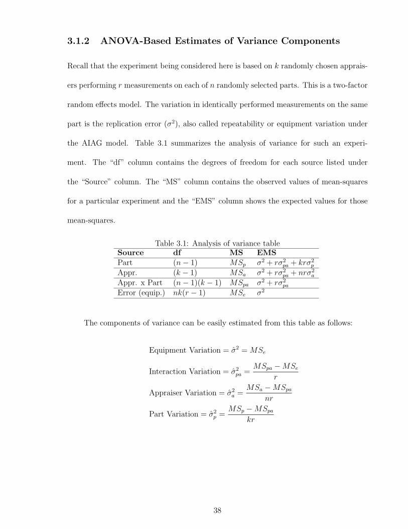
Recall that the experiment being considered here is based on k randomly chosen apprais-
ers performing r measurements on each of n randomly selected parts. This is a two-factor
random effects model. The variation in identically performed measurements on the same
part is the replication error (σ2), also called repeatability or equipment variation under
the AIAG model. Table 3.1 summarizes the analysis of variance for such an experi-
ment. The “df” column contains the degrees of freedom for each source listed under
the “Source” column. The “MS” column contains the observed values of mean-squares
for a particular experiment and the “EMS” column shows the expected values for those
mean-squares.
Table 3.1: Analysis of variance tableSource df MS EMSPart (n− 1) MSp σ2 + rσ2
pa + krσ2p
Appr. (k − 1) MSa σ2 + rσ2pa + nrσ2
a
Appr. x Part (n− 1)(k − 1) MSpa σ2 + rσ2pa
Error (equip.) nk(r − 1) MSe σ2
The components of variance can be easily estimated from this table as follows:
Equipment Variation = σ2 = MSe
Interaction Variation = σ2pa =
MSpa −MSe
r
Appraiser Variation = σ2a =
MSa −MSpa
nr
Part Variation = σ2p =
MSp −MSpa
kr
38
3.2 Accounting for Within-Appraiser Variation
Consider the linear model underlying the traditional MSA given in Eq(2.1). The term
βj represents appraiser bias. This model does not allow for any variation in this bias
associated with an appraiser. For example, consider an appraiser measuring the length
of a part, in millimeters, having a bias (βj) of −2mm. The current model assumes that
every time this appraiser measures a part, he/she will measure it exactly 2mm less than
the true value. The concept of within-appraiser variation is more realistic in that it
assumes βj to be only an average bias with a certain variation from reading to reading.
The relationship between variation among appraisers and variation within apprais-
ers is depicted in Figure 3.1 for three appraisers. The appraiser-to-appraiser variation,
σ2a, governs the variation in mean appraiser biases, the βjs. Hence, the jth appraiser
performs with a mean bias of βj. The bias associated with a particular measurement
on a given part has a variance of σ2aj
, which is the within-appraiser variation for the
jth appraiser. Under the traditional model, σ2aj
= 0 for all appraisers. The difficulty
in visually detecting (through control charts or residual plots) or estimating appraiser
inconsistency is primarily because it is confounded with equipment variation. Replica-
tion error, thus, has two components to it—equipment variation and within-appraiser
variation. In other words, εijm = γijm +νijm, where εijm represents replication error from
Eq(2.1) and γijm, νijm represent measurement error due to within-appraiser variation (for
appraiser j) and equipment variation, respectively. It is easy to see why equating repli-
cation error to equipment variation will overestimate the latter. The model in Eq(2.1)
39
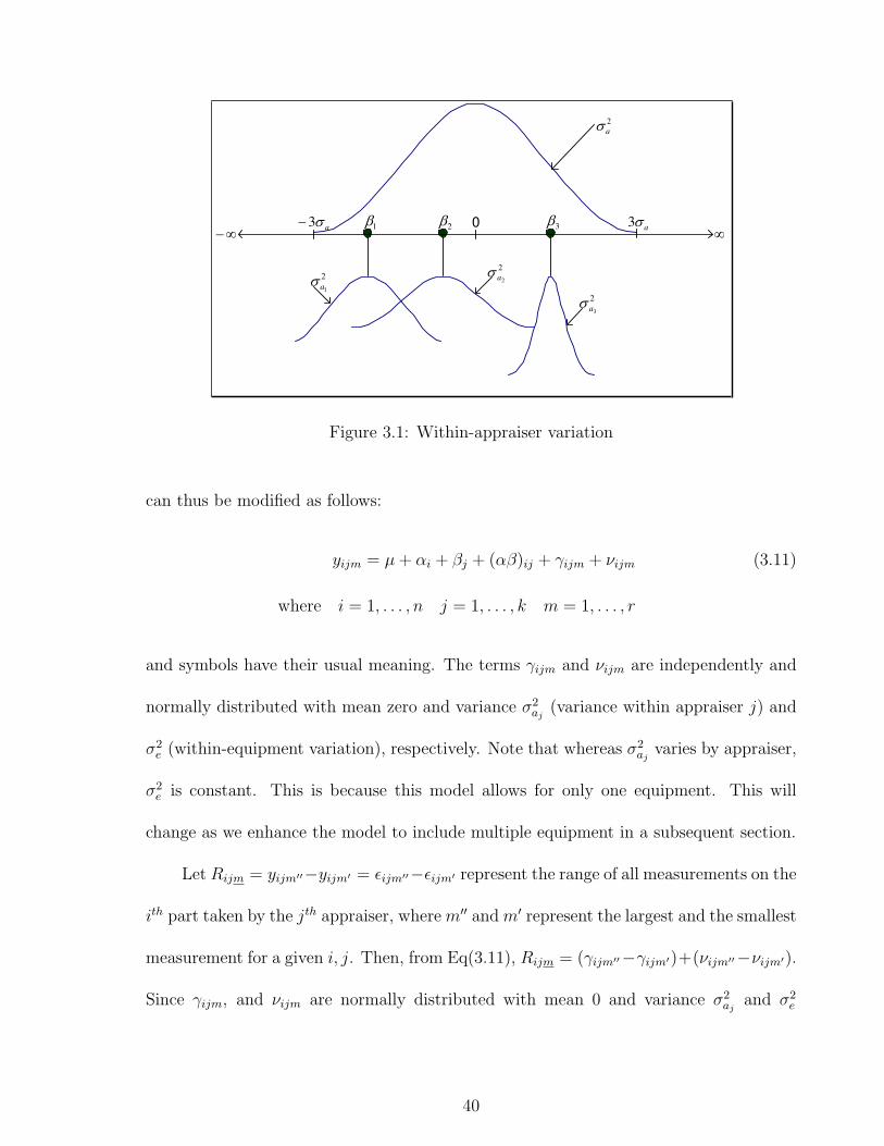
2
a
2
1a
2
2a
2
3a
1 2 30a
3a
3
Figure 3.1: Within-appraiser variation
can thus be modified as follows:
yijm = µ + αi + βj + (αβ)ij + γijm + νijm (3.11)
where i = 1, . . . , n j = 1, . . . , k m = 1, . . . , r
and symbols have their usual meaning. The terms γijm and νijm are independently and
normally distributed with mean zero and variance σ2aj
(variance within appraiser j) and
σ2e (within-equipment variation), respectively. Note that whereas σ2
ajvaries by appraiser,
σ2e is constant. This is because this model allows for only one equipment. This will
change as we enhance the model to include multiple equipment in a subsequent section.
Let Rijm = yijm′′−yijm′ = εijm′′−εijm′ represent the range of all measurements on the
ith part taken by the jth appraiser, where m′′ and m′ represent the largest and the smallest
measurement for a given i, j. Then, from Eq(3.11), Rijm = (γijm′′−γijm′)+(νijm′′−νijm′).
Since γijm, and νijm are normally distributed with mean 0 and variance σ2aj
and σ2e
40

respectively, we obtain,(
E
[Rijm
d2(r)
])2
= σ2j = σ2
aj+ σ2
e (3.12)
where σ2j is the replication error for the jth appraiser. The average of the ranges, Rijm,
taken over all parts for appraiser j, given by R.jm = 1n
∑ni=1(yijm′′ − yijm′) can be used
as an estimate of Rijm.
Since equipment and within-appraiser variation are confounded with each other, it
is difficult, if not impossible, to get a point estimate on them. It is, however, possible to
estimate the bounds on these quantities, as shown in the next subsection.
3.2.1 Estimating Bounds
From Eq(3.12), it is easy to see that the replication error for appraiser j, σ2j = σ2
aj+σ2
e . A
similar expression can be derived for each of k appraisers and can be collectively expressed
as Ak where the subscript indicates the number of equations in the set.
Ak =
σ2a1
+ σ2e = σ2
1
σ2a2
+ σ2e = σ2
2
...
σ2ak
+ σ2e = σ2
k
Assume that the equations are ordered such that σ21 > σ2
2 > . . . > σ2k. Let κ =
(k2
). If Ei
is the ith equation in Ak, then performing the operations Ei−Ei+x where i = 1, ..., (k−1)
and x = 1, ..., (k − i), gives us the following κ equations
Aκ =
σ2a1− σ2
a2= σ2
1 − σ22
σ2a1− σ2
a3= σ2
1 − σ23
...
σ2ak−1
− σ2ak
= σ2k−1 − σ2
k
41
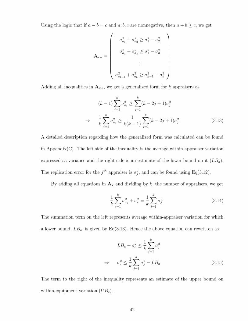
Using the logic that if a− b = c and a, b, c are nonnegative, then a + b ≥ c, we get
Aκ+ =
σ2a1
+ σ2a2≥ σ2
1 − σ22
σ2a1
+ σ2a3≥ σ2
1 − σ23
...
σ2ak−1
+ σ2ak≥ σ2
k−1 − σ2k
Adding all inequalities in Aκ+, we get a generalized form for k appraisers as
(k − 1)k∑
j=1
σ2aj≥
k∑j=1
(k − 2j + 1)σ2j
⇒ 1
k
k∑j=1
σ2aj≥ 1
k(k − 1)
k∑j=1
(k − 2j + 1)σ2j (3.13)
A detailed description regarding how the generalized form was calculated can be found
in Appendix(C). The left side of the inequality is the average within appraiser variation
expressed as variance and the right side is an estimate of the lower bound on it (LBa).
The replication error for the jth appraiser is σ2j , and can be found using Eq(3.12).
By adding all equations in Ak and dividing by k, the number of appraisers, we get
1
k
k∑j=1
σ2aj
+ σ2e =
1
k
k∑j=1
σ2j (3.14)
The summation term on the left represents average within-appraiser variation for which
a lower bound, LBa, is given by Eq(3.13). Hence the above equation can rewritten as
LBa + σ2e ≤
1
k
k∑j=1
σ2j
⇒ σ2e ≤
1
k
k∑j=1
σ2j − LBa (3.15)
The term to the right of the inequality represents an estimate of the upper bound on
within-equipment variation (UBe).
42
3.2.2 Estimating Trivial Bounds
As has been shown earlier, σ2j = σ2
aj+ σ2
e ∀j. Clearly, σ2e ≤ σ2
j ∀j, where the equality
holds when σ2aj
= 0. Hence σ2e ≤ minj(σ
2j ). In other words, UBeTriv = minj(σ
2j ) places an
upper bound on equipment variation. From Eq(3.14)and having an upper bound on σ2e
(UBeTriv) we have 1k
∑kj=1 σ2
aj≥ 1
k
∑kj=1 σ2
j −UBeTriv where the left side of the inequality
represents the average within-appraiser variation and the right side gives an estimated
lower bound on it (LBaTriv)
Recall that all of the estimates (LBa, UBe, LBaTriv, UBeTriv) have be derived using
expected values. When calculating an actual value for these estimates, estimates of these
expected values will be used. This causes the estimated bounds to be ineffective at times.
This will be discussed in more detail later.
3.3 Correcting the Estimate for PV
Consider the model given in Eq(2.1). The average of all measurements by all appraisers
on the ith part can be represented as
1
kr
k∑j=1
r∑m=1
yijm = yi.. = µ + αi + β. + (αβ)i. + εi..
The the range of yi.. over all parts is given by Ri.. = (αi′′−αi′)+(αβi′′.−αβi′.)+(εi′′..−εi′..).
As shown earlier,Ri..
d2(n)is traditionally used to estimate part variation, even though it
estimates not σ2p, but rather
(Ri..
d2(n)
)2
= σ2p +
σ2pa
k+
σ2e
kr(3.16)
Hence the correct estimate of PV is notRi..
d2(n), but rather σ2
p =(
Ri..
d2(n)
)2
− σ2pa
k− σ2
e
kr. As
mentioned previously, the range-based approach is appropriate when the additive model
43
is believed to adequately represent reality and hence, the interaction term can be ignored,
so that σ2pa = 0. The current estimate of process variation should still be adjusted for
σ2e
kr, the last term in Eq(3.16) and be given as
σ2p =
(Ri..
d2(n)
)2
− σ2e
kr
=⇒ σ2p =
(Ri..
d2(n)
)2
− 1
kr
(R..m
d2(r)
)2
=⇒ σ2p = max
(0,
(Ri..
d2(n)
)2
− 1
kr
(R..m
d2(r)
)2)
(3.17)
where, R..m = 1nk
∑ni=1
∑kj=1(maxm yijm − minm yijm) is the average of measurement
ranges over all parts and all appraisers. Under the traditional model,R..m
d2(r)is typically
used as EV to estimate σe, the equipment variation. The last equation follows because a
negative estimate of variance is usually replaced by zero and counted as a null estimate.
Under the traditional model (ignoring within-appraiser variation), the equation above
can be rewritten as PV 2new = PV 2
old − EV 2
kr.
3.4 On Using Multiple Equipment
As mentioned above, in a situation where multiple equipment or measuring devices of
the same type are routinely used for measurement, a significant equipment-to-equipment
variance component may exist. This is ignored under the current model and may result
in overestimating the true process variation. Once the decision to use multiple equipment
has been made, a decision as to whether equipment should be treated as a random or a
fixed factor should be made. This decision depends on the situation and on the objectives
of the study.
For example, if only a small and specific number of equipment are used during
44
routine measurements, then all equipment may be used in the study and equipment
may be treated as a fixed factor. The design would then be analyzed as a mixed model
assuming that parts and appraisers would still be random. Any interaction involving part
or appraiser would also be treated as random. The objective with respect to equipment,
however, should be to study the main effects of those specific equipment. Any attempt
to generalize the conclusions to the entire population of equipment (if larger than the
sample) will lead to erroneous conclusions. Besides, as mentioned earlier, Montgomery
and Runger (1994a) recommend that even in such a case, the factor should be treated as
a random sample from the potential population.
For now, equipment will be considered to be a random factor. The objective of the
study with respect to equipment would be to estimate the variance components due to
equipment. The linear model that retains all the provisions of the AIAG model, accounts
for within-appraiser variation and allows for multiple equipment to be used is given below:
yijlm = µ + αi + βj + ωl + αβij + αωil + βωjl + αβωijl + γijlm + νijlm (3.18)
where i = 1, . . . , n j = 1, . . . , k l = 1, . . . , q m = 1, . . . , r
and symbols have their usual meaning. The term ωl is the equipment effect and is
normally distributed with mean zero and variance σ2e . The terms αβij, αωil, and βωjl
represent two-way interactions between part and appraiser, part and equipment, and
appraiser and equipment, respectively. They are normally distributed with mean zero and
variance σ2pa, σ
2pe, and σ2
ae, respectively. The three-way interaction among part, appraiser
and equipment is denoted by αβωijl, and is normally distributed with mean zero and
variance σ2pae. The replication error is, as before, split into within-appraiser variation and
within-equipment variation. Since the latter can be different for different equipment, the
45
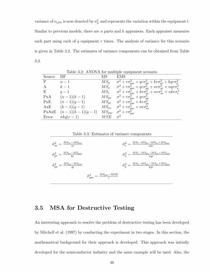
variance of νijlm is now denoted by σ2el
and represents the variation within the equipment l.
Similar to previous models, there are n parts and k appraisers. Each appraiser measures
each part using each of q equipment r times. The analysis of variance for this scenario
is given in Table 3.2. The estimates of variance components can be obtained from Table
3.3.
Table 3.2: ANOVA for multiple equipment scenarioSource DF MS EMSP n− 1 MSp σ2 + rσ2
pae + qrσ2pa + krσ2
pe + kqrσ2p
A k − 1 MSa σ2 + rσ2pae + qrσ2
pa + nrσ2ae + nqrσ2
a
E q − 1 MSe σ2 + rσ2pae + krσ2
pe + nrσ2ae + nkrσ2
e
PxA (n− 1)(k − 1) MSpa σ2 + rσ2pae + qrσ2
pa
PxE (n− 1)(q − 1) MSpe σ2 + rσ2pae + krσ2
pe
AxE (k − 1)(q − 1) MSae σ2 + rσ2pae + nrσ2
ae
PxAxE (n− 1)(k − 1)(q − 1) MSpae σ2 + rσ2pae
Error nkq(r − 1) MSE σ2
Table 3.3: Estimates of variance components
σ2ae = MSae−MSpae
nrσ2
e = MSe−MSpe−MSae+MSpae
nkr
σ2pe = MSpe−MSpae
krσ2
a = MSa−MSpa−MSae+MSpae
nqr
σ2pa = MSpa−MSpae
qrσ2
p = MSp−MSpa−MSpe+MSpae
kqr
σ2pae = MSpae−MSE
r
3.5 MSA for Destructive Testing
An interesting approach to resolve the problem of destructive testing has been developed
by Mitchell et al. (1997) by conducting the experiment in two stages. In this section, the
mathematical background for their approach is developed. This approach was initially
developed for the semiconductor industry and the same example will be used. Also, the
46
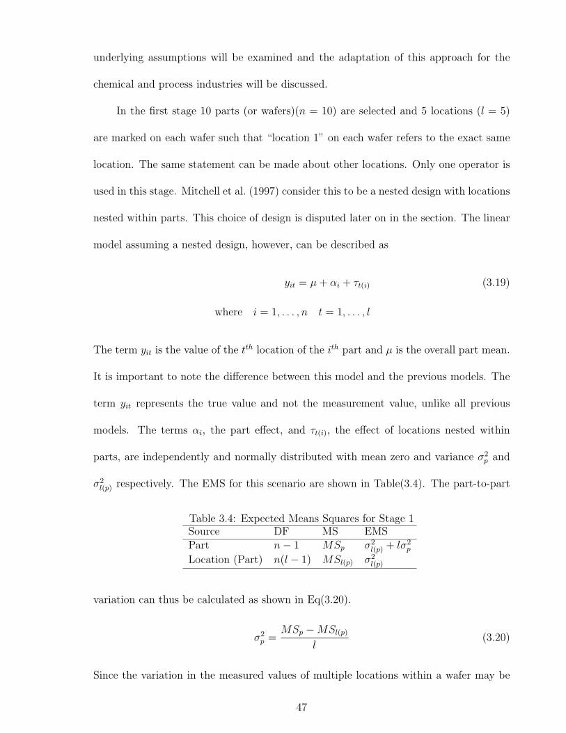
underlying assumptions will be examined and the adaptation of this approach for the
chemical and process industries will be discussed.
In the first stage 10 parts (or wafers)(n = 10) are selected and 5 locations (l = 5)
are marked on each wafer such that “location 1” on each wafer refers to the exact same
location. The same statement can be made about other locations. Only one operator is
used in this stage. Mitchell et al. (1997) consider this to be a nested design with locations
nested within parts. This choice of design is disputed later on in the section. The linear
model assuming a nested design, however, can be described as
yit = µ + αi + τt(i) (3.19)
where i = 1, . . . , n t = 1, . . . , l
The term yit is the value of the tth location of the ith part and µ is the overall part mean.
It is important to note the difference between this model and the previous models. The
term yit represents the true value and not the measurement value, unlike all previous
models. The terms αi, the part effect, and τt(i), the effect of locations nested within
parts, are independently and normally distributed with mean zero and variance σ2p and
σ2l(p) respectively. The EMS for this scenario are shown in Table(3.4). The part-to-part
Table 3.4: Expected Means Squares for Stage 1Source DF MS EMSPart n− 1 MSp σ2
l(p) + lσ2p
Location (Part) n(l − 1) MSl(p) σ2l(p)
variation can thus be calculated as shown in Eq(3.20).
σ2p =
MSp −MSl(p)
l(3.20)
Since the variation in the measured values of multiple locations within a wafer may be
47
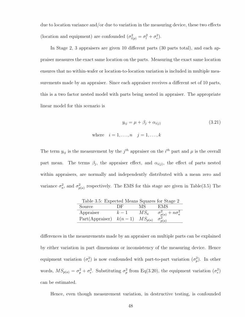
due to location variance and/or due to variation in the measuring device, these two effects
(location and equipment) are confounded (σ2l(p) = σ2
l + σ2e).
In Stage 2, 3 appraisers are given 10 different parts (30 parts total), and each ap-
praiser measures the exact same location on the parts. Measuring the exact same location
ensures that no within-wafer or location-to-location variation is included in multiple mea-
surements made by an appraiser. Since each appraiser receives a different set of 10 parts,
this is a two factor nested model with parts being nested in appraiser. The appropriate
linear model for this scenario is
yij = µ + βj + αi(j) (3.21)
where i = 1, . . . , n j = 1, . . . , k
The term yij is the measurement by the jth appraiser on the ith part and µ is the overall
part mean. The terms βj, the appraiser effect, and αi(j), the effect of parts nested
within appraisers, are normally and independently distributed with a mean zero and
variance σ2a, and σ2
p(a) respectively. The EMS for this stage are given in Table(3.5) The
Table 3.5: Expected Means Squares for Stage 2Source DF MS EMSAppraiser k − 1 MSa σ2
p(a) + nσ2a
Part(Appraiser) k(n− 1) MSp(a) σ2p(a)
differences in the measurements made by an appraiser on multiple parts can be explained
by either variation in part dimensions or inconsistency of the measuring device. Hence
equipment variation (σ2e) is now confounded with part-to-part variation (σ2
p). In other
words, MSp(a) = σ2p + σ2
e . Substituting σ2p from Eq(3.20), the equipment variation (σ2
e)
can be estimated.
Hence, even though measurement variation, in destructive testing, is confounded
48
with sample-to-sample variation, this approach developed by Mitchell et al. (1997) pro-
vides a very clever way of estimating it. This approach needs to be examined, however,
for the underlying assumptions and how those assumptions hold in various scenarios.
Also, it is necessary to show how this method can be adapted for chemical and process
industries and if this adaptation violates some of the underlying assumptions.
3.5.1 An In-Depth Look at the Process
From the description of Stage 2 of the experiment it appears that the difference in the
measurement of the same location on two parts by the same appraiser is attributed to
only equipment variation and part-to-part variation. The implicit assumption here is
that the “location effect” is constant for a given location regardless of the part. In
other words, if µ + αi + τt(i) be the true value of the tth location on the ith part and
µ + αi′ + τt(i′) be the true mean of the tth location on the i′th part, then this assumption
implies thatτt(i) = τt(i′). This is clearly in conflict with the model for Stage 1.
To see this more clearly, consider taking the range of 10 measurements made by an
appraiser in Stage 2. This range can be expressed as Rij = (yi′′j − yi′j) = (αi′′(j) − αi′(j))
such that i′′ and i′ refer to the parts with maximum and minimum measured value,
respectively. The corresponding variance can be expressed as
E
(Rij
d∗2(n)
)2
= σ2p(a) = MSp(a) = σ2
p + σ2e (3.22)
Now consider taking, based on Stage 1, the range of measurements of the tth location
on 10 parts by an appraiser. This range can be expressed as Rit = (yi′′t − yi′t) =
(αi′′ − αi′) + (τt(i′′) − τt(i′)) and the corresponding variance as
E
(Rit
d∗2(n)
)2
= σ2p + σ2
l(p) = σ2p + σ2
e + σ2l (3.23)
49
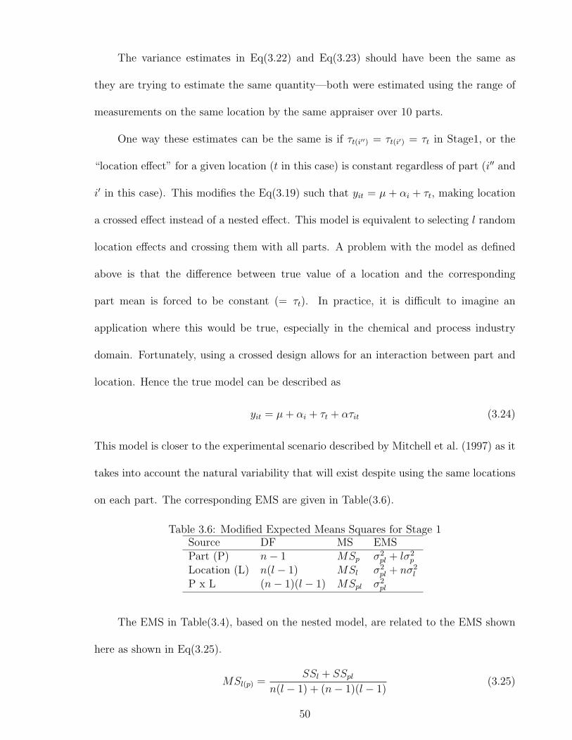
The variance estimates in Eq(3.22) and Eq(3.23) should have been the same as
they are trying to estimate the same quantity—both were estimated using the range of
measurements on the same location by the same appraiser over 10 parts.
One way these estimates can be the same is if τt(i′′) = τt(i′) = τt in Stage1, or the
“location effect” for a given location (t in this case) is constant regardless of part (i′′ and
i′ in this case). This modifies the Eq(3.19) such that yit = µ + αi + τt, making location
a crossed effect instead of a nested effect. This model is equivalent to selecting l random
location effects and crossing them with all parts. A problem with the model as defined
above is that the difference between true value of a location and the corresponding
part mean is forced to be constant (= τt). In practice, it is difficult to imagine an
application where this would be true, especially in the chemical and process industry
domain. Fortunately, using a crossed design allows for an interaction between part and
location. Hence the true model can be described as
yit = µ + αi + τt + ατit (3.24)
This model is closer to the experimental scenario described by Mitchell et al. (1997) as it
takes into account the natural variability that will exist despite using the same locations
on each part. The corresponding EMS are given in Table(3.6).
Table 3.6: Modified Expected Means Squares for Stage 1Source DF MS EMSPart (P) n− 1 MSp σ2
pl + lσ2p
Location (L) n(l − 1) MSl σ2pl + nσ2
l
P x L (n− 1)(l − 1) MSpl σ2pl
The EMS in Table(3.4), based on the nested model, are related to the EMS shown
here as shown in Eq(3.25).
MSl(p) =SSl + SSpl
n(l − 1) + (n− 1)(l − 1)(3.25)
50
where SS indicates Sum of Squares and subscripts have their usual meaning. The part-to-
part variation can be expressed as σ2p =
MSp−MSpl
land the location-to-location variation
as σ2l =
MSl−MSpl
n. Equipment variation, under this model, will be confounded with the
part-by-location interaction.
It is important to assess the impact of these changes to the model for Stage 1 on
the model for Stage 2. Since location effects are considered to be crossed, it may seem
like each measurement for Stage 2 should be expressed as yij = µ + βj + αi(j) + τt. But
since only one (and the same) location is being measured on each part (t = 1) in all cases
τt = τ1 is a constant. Hence µ, the unknown constant will automatically account for it.
Since n parts for each appraiser were chosen separately at random, it is correct to treat
part as a random factor nested within appraisers. No changes are required to the model
in Stage 2.
Independent of the discussion above, consider the fact that Mitchell et al. (1997)
state that in Stage 1, equipment variation is confounded with location-to-location varia-
tion. The argument that can be made in favor of this statement is that measured values
of various locations on the same part are different not only because true location di-
mensions are different (location effect) but also due the inconsistency of the measuring
device. However, it can just as easily be argued that equipment variation is confounded
with part-to-part variation—measured values on a particular location across different
parts are different not only due to differing part effects (and location effects) but also
due to inconsistent measuring device. In fact, this is the exact argument made in Stage
2 to claim the confounding of equipment variation with part-to-part variation. Only,
location effect is ignored in Stage 2 as explained above. The modification to the Stage
1 model suggested resolves this ambiguity by realizing that EV is essentially confounded
51

with part-by-location interaction and not with either part effect or location effect. This is
also consistent with the assumption of Stage 2 that EV is confounded with PV because,
by using only one location, the interaction manifests itself as PV.
The ideas presented here will be tested using simulation. Data would be simulated in
a manner consistent with Eq(3.24) for Stage 1 and Eq(3.21) for Stage 2. The VCs will be
estimated using both the approach given by Mitchell et al. (1997) and the modification
proposed above. Statistical tests will be performed to test the hypotheses that the
modified approach is significantly different from the old approach and that the VCs
estimated using both approaches are, on average, equal to the quantities being estimated.
A designed experiment will be simulated to evaluate the robustness of these hypotheses
across various combinations of PV, LV, EV and PL interaction.
3.6 Comparing Measurement System Acceptability
Criteria
Among all metrics that assess measurement system acceptability, precision-to-tolerance
ratio (PTR) is the only one that takes into account the specification range, or tolerance
of the product. While this makes PTR a unique metric, it introduces the potential
for inconsistency in conclusion when compared with other metrics. The tolerance of a
process and its variation have a definite link through the sigma capability of the process.
For example, in a Six-Sigma capable process, if the process standard deviation is given
by σp, the specs are µ ± 6σp, where µ is the process mean. Hence the tolerance is 12σp
and process span is 6σp (µ ± 3σp). The convention of 1.5σ shift in the process mean is
inconsequential to this discussion. If the sigma capability of a process is given by s, then
52

the tolerance of the process can be calculated as 2sσp.
The sigma capability of the process is used as a common platform for comparison
of these techniques. An arbitrary process standard deviation, say σp, will be selected.
The sigma capability of the process will then be used to calculate tolerance values. The
measurement standard deviation will then be systematically varied from extremely low
values to values larger than σp. For each scenario all metrics will be calculated, thus
revealing any systematic patterns or inconsistencies. The implementation of this part
will be in Microsoft Excel.
53
Chapter 4
The Simulation Process
Chapter Overview
The validity of the ideas presented in the previous chapter is tested through Monte Carlo
simulations of the measurement process using MATLAB as the programming language.
This chapter walks the reader through the simulation process by illustrating the output
of these programs at each step. This acts not only as a justification of the approach used
but allows the reader to gain appreciation for the analysis conducted and conclusions
drawn in the next chapter.
4.1 Introduction
There are four distinct areas into which this research can be divided— MSA with within-
appraiser variation, MSA using multiple devices, MSA for destructive testing, and com-
parison of measurement system acceptability criteria. The software developed essentially
consists of three different programs addressing each of the first three areas combined
into a single application. This section provides a brief overview of each of these and the
subsequent sections discuss each program in more detail.
The first program allows the user to include within-appraiser variation. It estimates
variance components using the traditional approach and the one recognizing the existence
54
of within-appraiser variation. The latter estimates lower bounds for within-appraiser vari-
ation and upper bounds for equipment variation using two different approaches discussed
in Chapter 3. Range-based estimates of variance components are typically considered to
be inferior to ANOVA-based estimates. This program calculates both, allowing for a
comparison between the two. In addition, this program calculates discrimination ratio
and number of distinct data categories and compares them. It also calculates Appraiser
Variation using a different approach suggested by Montgomery and Runger (1994a).
The second program works under the assumption that the measurement process is
destructive. It tests and extends the approach suggested by Mitchell et al. (1997).
The third program extends the traditional model to include multiple measuring
devices. It uses a three-way random effects model (instead of a traditional two-way
model), hence adding a component of variation.
The general approach used to generate data in these programs is very similar and
is shown in the form of a flow chart in Fig(4.1). It starts with taking an arbitrary part
mean (input from the user) and generates true part dimensions by adding part-to-part
variation to it. Next, each component of variation—appraiser, replication, equipment
etc., is added to the data in a stepwise manner. When the data are ready in a form that
would be available if true part dimensions were not known, various estimation approaches
are used to estimate the variance components of interest. Eventually these estimates will
be compared to the true value being estimated.
55
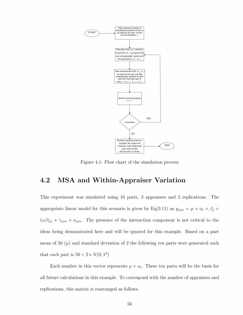
Take maximum number of
simulations (maxSim) to be run
as input by the user. Let the
current simulation = i
START
Take part mean ( ), and part-
to-part SD (p
) as input by the
user and generate n parts such
that each part is +1
zp
Take measurement SDs (ea
, )
as input by the user and add
measurement variation to each
part such that each part is
now +1
zp
+2
za
+3
ze
Set the current simulation
i = i + 1
i<maxSim
YES
Perform statistical tests to
compare the improved
estimates with traditional
ones and test the
effectiveness of both.
NO
END
Figure 4.1: Flow chart of the simulation process
4.2 MSA and Within-Appraiser Variation
This experiment was simulated using 10 parts, 3 appraisers and 2 replications. The
appropriate linear model for this scenario is given by Eq(3.11) as yijm = µ + αi + βj +
(αβ)ij + γijm + νijm. The presence of the interaction component is not critical to the
ideas being demonstrated here and will be ignored for this example. Based on a part
mean of 50 (µ) and standard deviation of 2 the following ten parts were generated such
that each part is 50 + 2 ∗N(0, 12)
Each number in this vector represents µ + αi. These ten parts will be the basis for
all future calculations in this example. To correspond with the number of appraisers and
replications, this matrix is rearranged as follows.
56
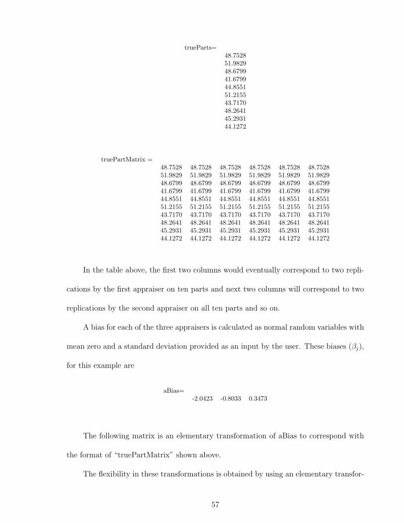
trueParts=48.752851.982948.679941.679944.855151.215543.717048.264145.293144.1272
truePartMatrix =48.7528 48.7528 48.7528 48.7528 48.7528 48.752851.9829 51.9829 51.9829 51.9829 51.9829 51.982948.6799 48.6799 48.6799 48.6799 48.6799 48.679941.6799 41.6799 41.6799 41.6799 41.6799 41.679944.8551 44.8551 44.8551 44.8551 44.8551 44.855151.2155 51.2155 51.2155 51.2155 51.2155 51.215543.7170 43.7170 43.7170 43.7170 43.7170 43.717048.2641 48.2641 48.2641 48.2641 48.2641 48.264145.2931 45.2931 45.2931 45.2931 45.2931 45.293144.1272 44.1272 44.1272 44.1272 44.1272 44.1272
In the table above, the first two columns would eventually correspond to two repli-
cations by the first appraiser on ten parts and next two columns will correspond to two
replications by the second appraiser on all ten parts and so on.
A bias for each of the three appraisers is calculated as normal random variables with
mean zero and a standard deviation provided as an input by the user. These biases (βj),
for this example are
aBias=-2.0423 -0.8033 0.3473
The following matrix is an elementary transformation of aBias to correspond with
the format of “truePartMatrix” shown above.
The flexibility in these transformations is obtained by using an elementary transfor-
57
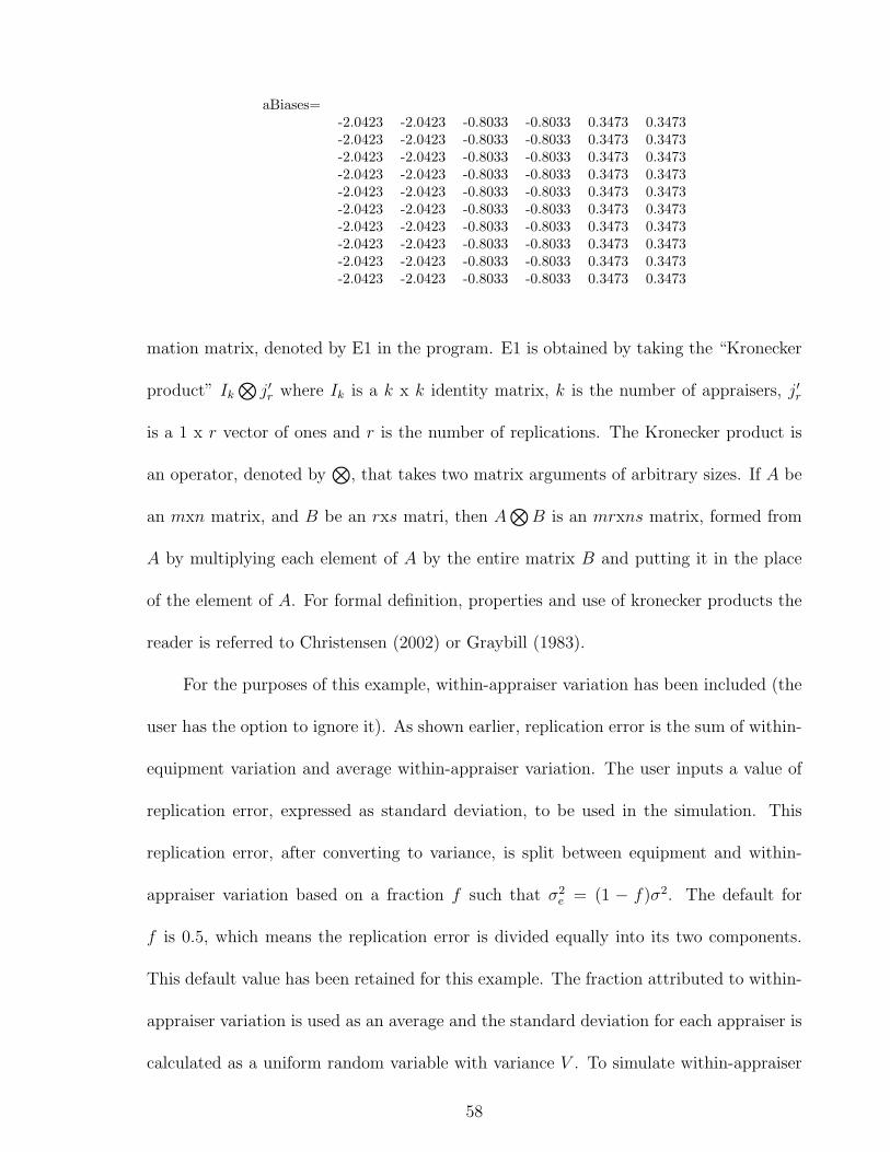
aBiases=-2.0423 -2.0423 -0.8033 -0.8033 0.3473 0.3473-2.0423 -2.0423 -0.8033 -0.8033 0.3473 0.3473-2.0423 -2.0423 -0.8033 -0.8033 0.3473 0.3473-2.0423 -2.0423 -0.8033 -0.8033 0.3473 0.3473-2.0423 -2.0423 -0.8033 -0.8033 0.3473 0.3473-2.0423 -2.0423 -0.8033 -0.8033 0.3473 0.3473-2.0423 -2.0423 -0.8033 -0.8033 0.3473 0.3473-2.0423 -2.0423 -0.8033 -0.8033 0.3473 0.3473-2.0423 -2.0423 -0.8033 -0.8033 0.3473 0.3473-2.0423 -2.0423 -0.8033 -0.8033 0.3473 0.3473
mation matrix, denoted by E1 in the program. E1 is obtained by taking the “Kronecker
product” Ik
⊗j′r where Ik is a k x k identity matrix, k is the number of appraisers, j′r
is a 1 x r vector of ones and r is the number of replications. The Kronecker product is
an operator, denoted by⊗
, that takes two matrix arguments of arbitrary sizes. If A be
an mxn matrix, and B be an rxs matri, then A⊗
B is an mrxns matrix, formed from
A by multiplying each element of A by the entire matrix B and putting it in the place
of the element of A. For formal definition, properties and use of kronecker products the
reader is referred to Christensen (2002) or Graybill (1983).
For the purposes of this example, within-appraiser variation has been included (the
user has the option to ignore it). As shown earlier, replication error is the sum of within-
equipment variation and average within-appraiser variation. The user inputs a value of
replication error, expressed as standard deviation, to be used in the simulation. This
replication error, after converting to variance, is split between equipment and within-
appraiser variation based on a fraction f such that σ2e = (1 − f)σ2. The default for
f is 0.5, which means the replication error is divided equally into its two components.
This default value has been retained for this example. The fraction attributed to within-
appraiser variation is used as an average and the standard deviation for each appraiser is
calculated as a uniform random variable with variance V . To simulate within-appraiser
58

variation, a variation is added to each measurement made by an appraiser based on their
corresponding standard deviation. The matrix “wiav” shows these values in a format that
corresponds with the “truePartMatrix”. These values represent γijm. If the user chooses
to use the traditional model, which does not account for within-appraiser variation, these
values will all be zeros.
wiav =-0.4544 1.0205 3.8563 0.9547 0.0415 3.23774.1638 -0.0516 -2.7213 0.3244 3.8858 3.7676-0.9602 -2.2705 0.4105 5.6130 -3.3534 2.9544-5.9380 8.3592 -0.4223 -0.8355 -3.3497 6.08250.0381 -1.0080 -3.5332 6.7195 -0.9340 1.51870.2793 -5.5154 3.5950 4.5814 -0.0950 -3.12461.2386 6.9263 -0.0469 -5.9072 1.2948 -0.69331.9558 1.2738 1.6285 -5.1038 4.9135 -11.37035.0011 -4.3787 -2.1758 -1.7418 2.8863 2.1974-2.1436 2.4274 -1.9909 -0.5643 -8.1278 0.5430
Similarly replication errors (νijm) calculated based on the standard deviation input
from user are shown by matrix “ev”.
ev=-1.1822 2.5851 2.1678 -2.2490 -0.8936 -1.3398-1.3094 0.8818 -1.9624 3.4714 2.1642 2.6819-2.1613 2.5619 -1.3770 3.8749 4.7453 0.7762-0.0955 -0.9955 2.6790 3.2701 0.4586 0.78610.7587 -2.2374 -1.8185 -2.5119 -0.5332 -3.4147-0.6607 1.6153 -0.8257 -0.4271 1.4033 0.4557-0.9998 0.0824 -1.0123 -0.3979 -0.9752 1.3713-0.0720 -1.5124 3.2395 0.6150 3.7250 -1.2736-0.3495 -0.1783 0.1618 -1.1447 2.2137 -2.0052-1.9145 -4.0177 -2.1621 -1.9553 -2.4551 -0.3712
The final measurements calculated as the sum of truePartMatrix, aBiases, repEr-
rors and wiav are shown as matrix “measurements”. These measurements represent
µ + αi + βj + γijm + νijm. These measurements can now be used for estimating vari-
ous components of variance using both range-based and ANOVA-based approaches. In
59
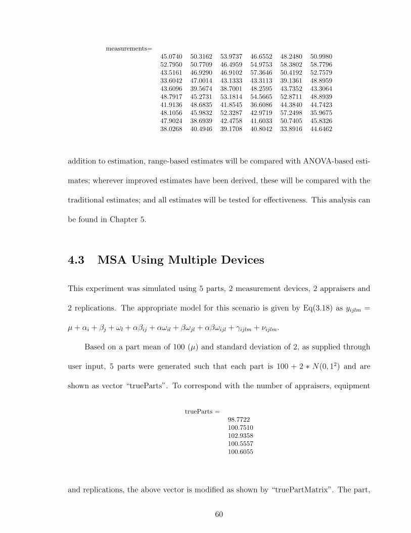
measurements=45.0740 50.3162 53.9737 46.6552 48.2480 50.998052.7950 50.7709 46.4959 54.9753 58.3802 58.779643.5161 46.9290 46.9102 57.3646 50.4192 52.757933.6042 47.0014 43.1333 43.3113 39.1361 48.895943.6096 39.5674 38.7001 48.2595 43.7352 43.306448.7917 45.2731 53.1814 54.5665 52.8711 48.893941.9136 48.6835 41.8545 36.6086 44.3840 44.742348.1056 45.9832 52.3287 42.9719 57.2498 35.967547.9024 38.6939 42.4758 41.6033 50.7405 45.832638.0268 40.4946 39.1708 40.8042 33.8916 44.6462
addition to estimation, range-based estimates will be compared with ANOVA-based esti-
mates; wherever improved estimates have been derived, these will be compared with the
traditional estimates; and all estimates will be tested for effectiveness. This analysis can
be found in Chapter 5.
4.3 MSA Using Multiple Devices
This experiment was simulated using 5 parts, 2 measurement devices, 2 appraisers and
2 replications. The appropriate model for this scenario is given by Eq(3.18) as yijlm =
µ + αi + βj + ωl + αβij + αωil + βωjl + αβωijl + γijlm + νijlm.
Based on a part mean of 100 (µ) and standard deviation of 2, as supplied through
user input, 5 parts were generated such that each part is 100 + 2 ∗ N(0, 12) and are
shown as vector “trueParts”. To correspond with the number of appraisers, equipment
trueParts =98.7722100.7510102.9358100.5557100.6055
and replications, the above vector is modified as shown by “truePartMatrix”. The part,
60
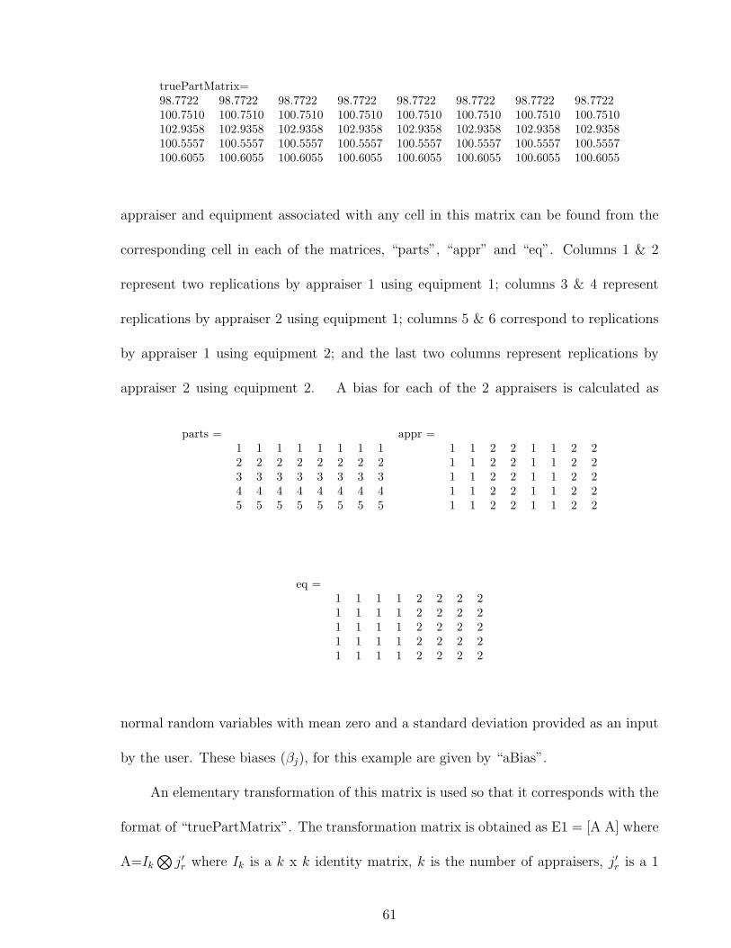
truePartMatrix=98.7722 98.7722 98.7722 98.7722 98.7722 98.7722 98.7722 98.7722100.7510 100.7510 100.7510 100.7510 100.7510 100.7510 100.7510 100.7510102.9358 102.9358 102.9358 102.9358 102.9358 102.9358 102.9358 102.9358100.5557 100.5557 100.5557 100.5557 100.5557 100.5557 100.5557 100.5557100.6055 100.6055 100.6055 100.6055 100.6055 100.6055 100.6055 100.6055
appraiser and equipment associated with any cell in this matrix can be found from the
corresponding cell in each of the matrices, “parts”, “appr” and “eq”. Columns 1 & 2
represent two replications by appraiser 1 using equipment 1; columns 3 & 4 represent
replications by appraiser 2 using equipment 1; columns 5 & 6 correspond to replications
by appraiser 1 using equipment 2; and the last two columns represent replications by
appraiser 2 using equipment 2. A bias for each of the 2 appraisers is calculated as
parts = appr =1 1 1 1 1 1 1 1 1 1 2 2 1 1 2 22 2 2 2 2 2 2 2 1 1 2 2 1 1 2 23 3 3 3 3 3 3 3 1 1 2 2 1 1 2 24 4 4 4 4 4 4 4 1 1 2 2 1 1 2 25 5 5 5 5 5 5 5 1 1 2 2 1 1 2 2
eq =1 1 1 1 2 2 2 21 1 1 1 2 2 2 21 1 1 1 2 2 2 21 1 1 1 2 2 2 21 1 1 1 2 2 2 2
normal random variables with mean zero and a standard deviation provided as an input
by the user. These biases (βj), for this example are given by “aBias”.
An elementary transformation of this matrix is used so that it corresponds with the
format of “truePartMatrix”. The transformation matrix is obtained as E1 = [A A] where
A=Ik
⊗j′r where Ik is a k x k identity matrix, k is the number of appraisers, j′r is a 1
61
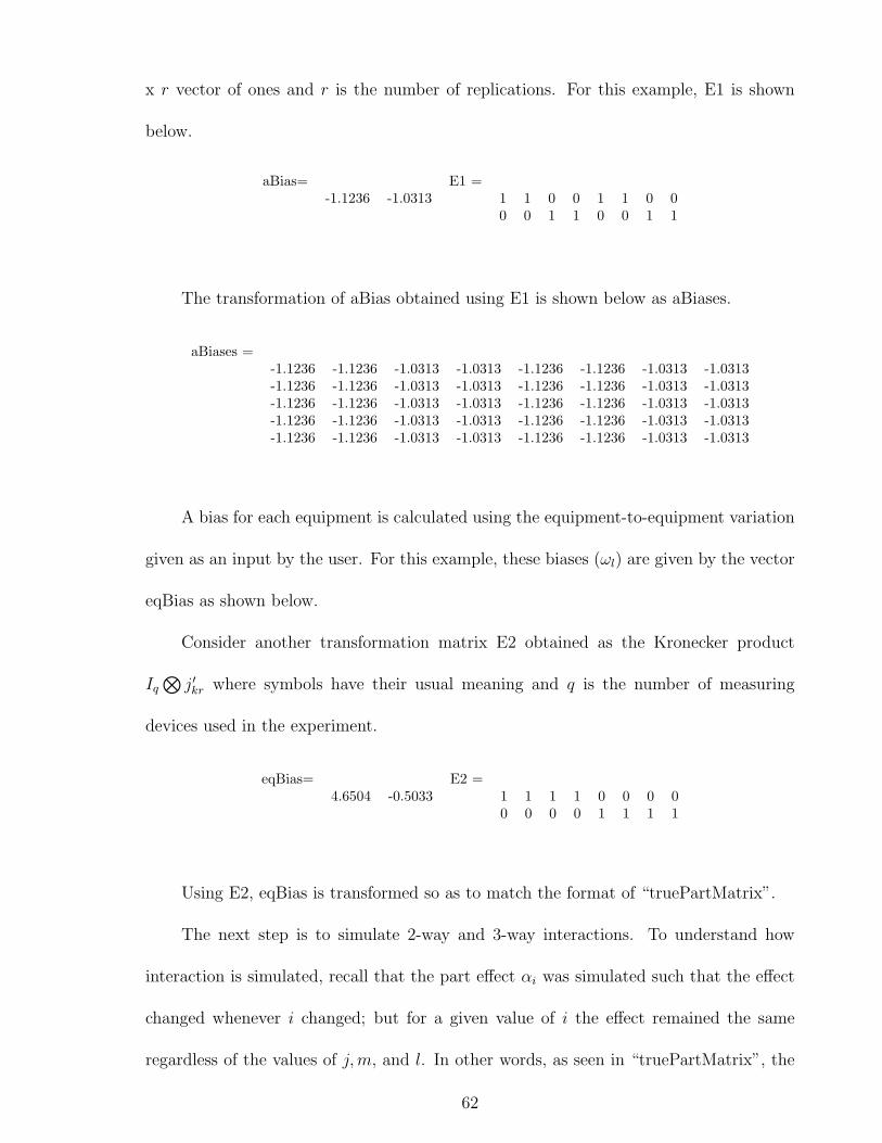
x r vector of ones and r is the number of replications. For this example, E1 is shown
below.
aBias= E1 =-1.1236 -1.0313 1 1 0 0 1 1 0 0
0 0 1 1 0 0 1 1
The transformation of aBias obtained using E1 is shown below as aBiases.
aBiases =-1.1236 -1.1236 -1.0313 -1.0313 -1.1236 -1.1236 -1.0313 -1.0313-1.1236 -1.1236 -1.0313 -1.0313 -1.1236 -1.1236 -1.0313 -1.0313-1.1236 -1.1236 -1.0313 -1.0313 -1.1236 -1.1236 -1.0313 -1.0313-1.1236 -1.1236 -1.0313 -1.0313 -1.1236 -1.1236 -1.0313 -1.0313-1.1236 -1.1236 -1.0313 -1.0313 -1.1236 -1.1236 -1.0313 -1.0313
A bias for each equipment is calculated using the equipment-to-equipment variation
given as an input by the user. For this example, these biases (ωl) are given by the vector
eqBias as shown below.
Consider another transformation matrix E2 obtained as the Kronecker product
Iq
⊗j′kr where symbols have their usual meaning and q is the number of measuring
devices used in the experiment.
eqBias= E2 =4.6504 -0.5033 1 1 1 1 0 0 0 0
0 0 0 0 1 1 1 1
Using E2, eqBias is transformed so as to match the format of “truePartMatrix”.
The next step is to simulate 2-way and 3-way interactions. To understand how
interaction is simulated, recall that the part effect αi was simulated such that the effect
changed whenever i changed; but for a given value of i the effect remained the same
regardless of the values of j, m, and l. In other words, as seen in “truePartMatrix”, the
62
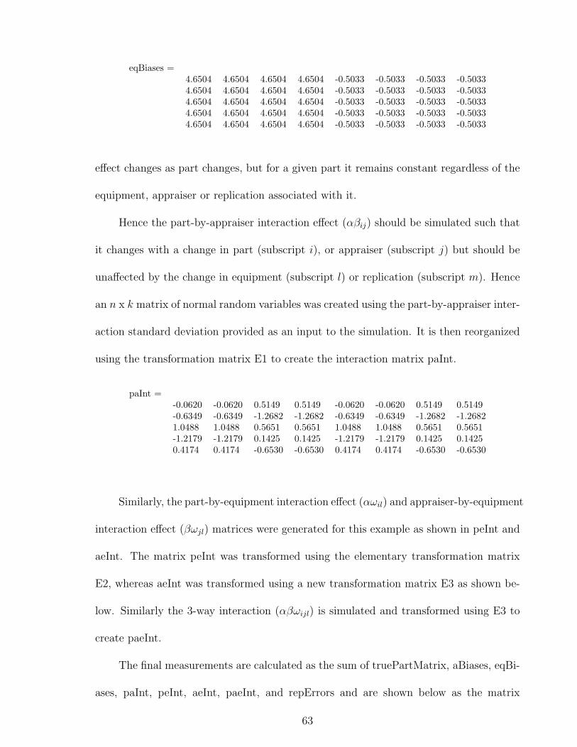
eqBiases =4.6504 4.6504 4.6504 4.6504 -0.5033 -0.5033 -0.5033 -0.50334.6504 4.6504 4.6504 4.6504 -0.5033 -0.5033 -0.5033 -0.50334.6504 4.6504 4.6504 4.6504 -0.5033 -0.5033 -0.5033 -0.50334.6504 4.6504 4.6504 4.6504 -0.5033 -0.5033 -0.5033 -0.50334.6504 4.6504 4.6504 4.6504 -0.5033 -0.5033 -0.5033 -0.5033
effect changes as part changes, but for a given part it remains constant regardless of the
equipment, appraiser or replication associated with it.
Hence the part-by-appraiser interaction effect (αβij) should be simulated such that
it changes with a change in part (subscript i), or appraiser (subscript j) but should be
unaffected by the change in equipment (subscript l) or replication (subscript m). Hence
an n x k matrix of normal random variables was created using the part-by-appraiser inter-
action standard deviation provided as an input to the simulation. It is then reorganized
using the transformation matrix E1 to create the interaction matrix paInt.
paInt =-0.0620 -0.0620 0.5149 0.5149 -0.0620 -0.0620 0.5149 0.5149-0.6349 -0.6349 -1.2682 -1.2682 -0.6349 -0.6349 -1.2682 -1.26821.0488 1.0488 0.5651 0.5651 1.0488 1.0488 0.5651 0.5651-1.2179 -1.2179 0.1425 0.1425 -1.2179 -1.2179 0.1425 0.14250.4174 0.4174 -0.6530 -0.6530 0.4174 0.4174 -0.6530 -0.6530
Similarly, the part-by-equipment interaction effect (αωil) and appraiser-by-equipment
interaction effect (βωjl) matrices were generated for this example as shown in peInt and
aeInt. The matrix peInt was transformed using the elementary transformation matrix
E2, whereas aeInt was transformed using a new transformation matrix E3 as shown be-
low. Similarly the 3-way interaction (αβωijl) is simulated and transformed using E3 to
create paeInt.
The final measurements are calculated as the sum of truePartMatrix, aBiases, eqBi-
ases, paInt, peInt, aeInt, paeInt, and repErrors and are shown below as the matrix
63
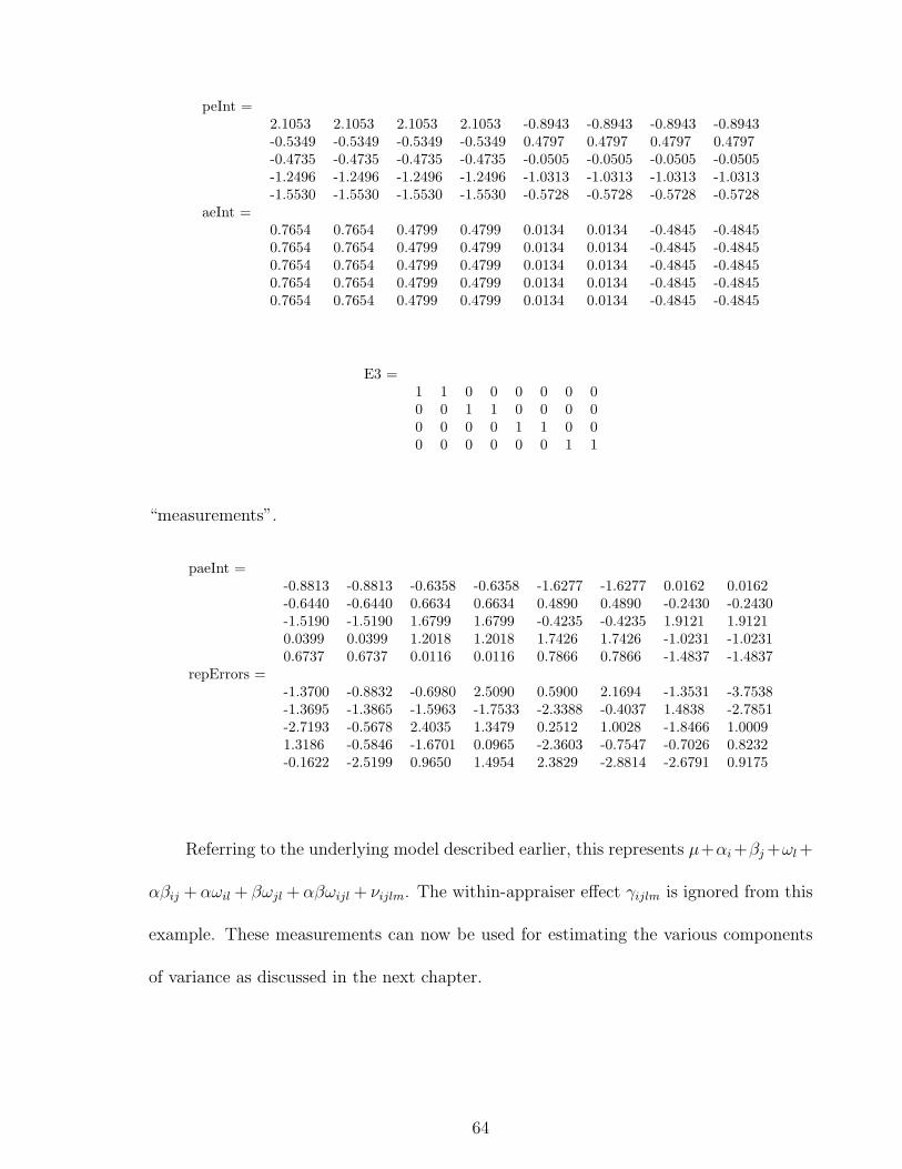
peInt =2.1053 2.1053 2.1053 2.1053 -0.8943 -0.8943 -0.8943 -0.8943-0.5349 -0.5349 -0.5349 -0.5349 0.4797 0.4797 0.4797 0.4797-0.4735 -0.4735 -0.4735 -0.4735 -0.0505 -0.0505 -0.0505 -0.0505-1.2496 -1.2496 -1.2496 -1.2496 -1.0313 -1.0313 -1.0313 -1.0313-1.5530 -1.5530 -1.5530 -1.5530 -0.5728 -0.5728 -0.5728 -0.5728
aeInt =0.7654 0.7654 0.4799 0.4799 0.0134 0.0134 -0.4845 -0.48450.7654 0.7654 0.4799 0.4799 0.0134 0.0134 -0.4845 -0.48450.7654 0.7654 0.4799 0.4799 0.0134 0.0134 -0.4845 -0.48450.7654 0.7654 0.4799 0.4799 0.0134 0.0134 -0.4845 -0.48450.7654 0.7654 0.4799 0.4799 0.0134 0.0134 -0.4845 -0.4845
E3 =1 1 0 0 0 0 0 00 0 1 1 0 0 0 00 0 0 0 1 1 0 00 0 0 0 0 0 1 1
“measurements”.
paeInt =-0.8813 -0.8813 -0.6358 -0.6358 -1.6277 -1.6277 0.0162 0.0162-0.6440 -0.6440 0.6634 0.6634 0.4890 0.4890 -0.2430 -0.2430-1.5190 -1.5190 1.6799 1.6799 -0.4235 -0.4235 1.9121 1.91210.0399 0.0399 1.2018 1.2018 1.7426 1.7426 -1.0231 -1.02310.6737 0.6737 0.0116 0.0116 0.7866 0.7866 -1.4837 -1.4837
repErrors =-1.3700 -0.8832 -0.6980 2.5090 0.5900 2.1694 -1.3531 -3.7538-1.3695 -1.3865 -1.5963 -1.7533 -2.3388 -0.4037 1.4838 -2.7851-2.7193 -0.5678 2.4035 1.3479 0.2512 1.0028 -1.8466 1.00091.3186 -0.5846 -1.6701 0.0965 -2.3603 -0.7547 -0.7026 0.8232-0.1622 -2.5199 0.9650 1.4954 2.3829 -2.8814 -2.6791 0.9175
Referring to the underlying model described earlier, this represents µ+αi +βj +ωl +
αβij + αωil + βωjl + αβωijl + νijlm. The within-appraiser effect γijlm is ignored from this
example. These measurements can now be used for estimating the various components
of variance as discussed in the next chapter.
64
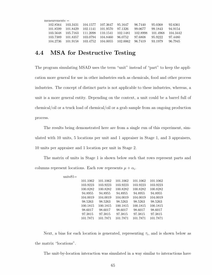
measurements =102.8564 103.3431 104.1577 107.3647 95.1647 96.7440 95.0368 92.6361101.8599 101.8429 102.1141 101.9570 97.1326 99.0677 99.1843 94.9154103.5648 105.7163 111.2098 110.1541 102.1481 102.8998 101.4968 104.3442103.7389 101.8357 103.0794 104.8460 96.0752 97.6808 95.9222 97.4480104.2736 101.9158 103.4752 104.0055 102.0062 96.7419 93.1979 96.7945
4.4 MSA for Destructive Testing
The program simulating MSAD uses the term “unit” instead of “part” to keep the appli-
cation more general for use in other industries such as chemicals, food and other process
industries. The concept of distinct parts is not applicable to these industries, whereas, a
unit is a more general entity. Depending on the context, a unit could be a barrel full of
chemical/oil or a truck load of chemical/oil or a grab sample from an ongoing production
process.
The results being demonstrated here are from a single run of this experiment, sim-
ulated with 10 units, 5 locations per unit and 1 appraiser in Stage 1, and 3 appraisers,
10 units per appraiser and 1 location per unit in Stage 2.
The matrix of units in Stage 1 is shown below such that rows represent parts and
columns represent locations. Each row represents µ + αi.
unitsS1=101.1062 101.1062 101.1062 101.1062 101.1062103.9223 103.9223 103.9223 103.9223 103.9223100.8282 100.8282 100.8282 100.8282 100.828294.8955 94.8955 94.8955 94.8955 94.8955104.0019 104.0019 104.0019 104.0019 104.001998.5263 98.5263 98.5263 98.5263 98.5263100.1815 100.1815 100.1815 100.1815 100.181598.6017 98.6017 98.6017 98.6017 98.601797.3815 97.3815 97.3815 97.3815 97.3815101.7871 101.7871 101.7871 101.7871 101.7871
Next, a bias for each location is generated, representing τt, and is shown below as
the matrix “locations”.
The unit-by-location interaction was simulated in a way similar to interactions have
65
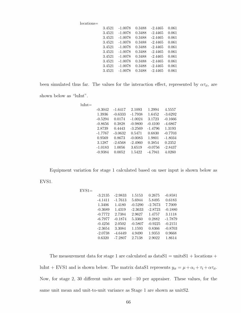
locations=3.4521 -1.0078 0.3488 -2.4465 0.0613.4521 -1.0078 0.3488 -2.4465 0.0613.4521 -1.0078 0.3488 -2.4465 0.0613.4521 -1.0078 0.3488 -2.4465 0.0613.4521 -1.0078 0.3488 -2.4465 0.0613.4521 -1.0078 0.3488 -2.4465 0.0613.4521 -1.0078 0.3488 -2.4465 0.0613.4521 -1.0078 0.3488 -2.4465 0.0613.4521 -1.0078 0.3488 -2.4465 0.0613.4521 -1.0078 0.3488 -2.4465 0.061
been simulated thus far. The values for the interaction effect, represented by ατit, are
shown below as “luInt”.
luInt=-0.3042 -1.6417 2.1093 1.2994 4.55571.3936 -0.6333 -1.7938 1.6452 -3.6292-0.5294 0.0174 -1.0024 3.1723 -0.1666-0.8656 0.3828 -0.9800 -0.4100 -4.68672.8739 0.4443 -3.2569 -1.4796 1.3193-1.7767 -3.0632 0.5471 0.6830 -0.77030.9569 0.8673 -0.0083 1.9801 -1.80343.1287 -2.6568 -2.4960 0.3854 0.2352-1.0183 1.0056 3.6519 -0.0756 -2.8437-0.9384 0.0052 1.5422 -4.7941 4.0260
Equipment variation for stage 1 calculated based on user input is shown below as
EVS1.
EVS1=-3.2135 -2.9833 1.5153 0.2675 -0.8581-4.1411 -1.7613 5.6944 5.8495 0.61831.3406 1.4180 -0.5290 -2.7673 7.7009-0.3689 1.4319 -2.3633 -2.8723 -0.1880-0.7772 2.7384 2.9627 1.4757 3.1118-6.7977 -0.1874 5.3360 0.2882 -1.7879-0.4256 2.0502 -0.5807 -0.9225 -0.2151-2.3654 3.3084 1.1593 0.8366 -0.8703-2.0738 -4.6449 4.9490 1.9353 0.96680.6320 -7.2807 2.7138 2.9022 1.8614
The measurement data for stage 1 are calculated as dataS1 = unitsS1 + locations +
luInt + EVS1 and is shown below. The matrix dataS1 represents yit = µ+αi + τt +ατit.
Now, for stage 2, 30 different units are used—10 per appraiser. These values, for the
same unit mean and unit-to-unit variance as Stage 1 are shown as unitS2.
66

dataS1=101.0407 95.4735 105.0795 100.2267 104.8649104.6269 100.5199 108.1716 108.9705 100.9723105.0915 101.2559 99.6456 98.7868 108.423597.1132 95.7025 91.901 89.1668 90.0818109.5508 106.1768 104.0565 101.5515 108.49493.4041 94.2679 104.7581 97.0511 96.0292104.165 102.0912 99.9413 98.7927 98.2241102.8172 98.2455 97.6137 97.3772 98.027697.7415 92.7344 106.3311 96.7947 95.5657104.9328 93.5037 106.3918 97.4487 107.7354
unitsS2=95.4994 98.2792 102.374199.9099 97.2776 102.0766101.6439 100.8262 103.006999.1996 103.179 95.844897.2365 100.3442 98.445399.0923 99.9631 99.8296.7974 99.7633 95.549293.2081 100.4245 102.951696.3031 101.8382 99.6154104.9658 101.0014 104.6096
The biases of each appraiser are shown below as apprBiases and the equipment
variation for this stage as EVS2.
apprBiases= EVS2=4.3103 -1.5316 -3.1774 -7.5696 -4.0317 5.85624.3103 -1.5316 -3.1774 2.4576 -2.301 -3.03364.3103 -1.5316 -3.1774 2.4576 -2.301 -3.03364.3103 -1.5316 -3.1774 0.8135 1.0809 3.06644.3103 -1.5316 -3.1774 1.6084 6.299 0.32254.3103 -1.5316 -3.1774 -1.2671 -1.3991 6.29934.3103 -1.5316 -3.1774 -1.8971 -2.3282 2.0024.3103 -1.5316 -3.1774 0.3366 5.6315 0.43054.3103 -1.5316 -3.1774 -3.7478 -3.3536 -1.99644.3103 -1.5316 -3.1774 -3.9796 0.4488 4.1241
The measurement data for stage 2 are calculated as dataS2 = unitsS2 + apprBiases
+ EVS2 and is shown below. The matrix dataS2 represents yij = µ + βj + αi(j).
The measurement data in dataS1 and dataS2 can now be used to estimate the EV
and AV. This will be discussed in the next chapter.
67

dataS2=92.24 92.7159 105.053
104.5486 93.8848 94.9325108.4117 96.9937 96.7959104.3233 102.7283 95.7338103.1551 105.1117 95.5904102.1355 97.0324 102.941999.2106 95.9035 94.373997.8549 104.5245 100.204696.8656 96.953 94.4416105.2964 99.9187 105.5563
68
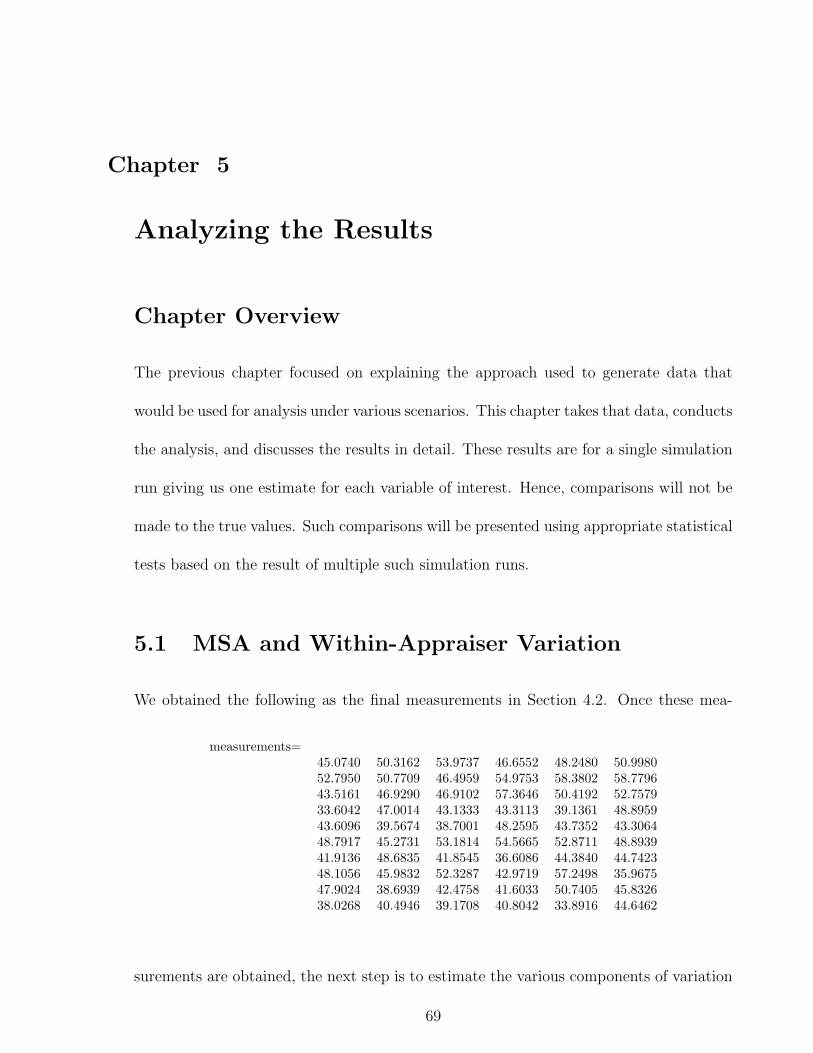
Chapter 5
Analyzing the Results
Chapter Overview
The previous chapter focused on explaining the approach used to generate data that
would be used for analysis under various scenarios. This chapter takes that data, conducts
the analysis, and discusses the results in detail. These results are for a single simulation
run giving us one estimate for each variable of interest. Hence, comparisons will not be
made to the true values. Such comparisons will be presented using appropriate statistical
tests based on the result of multiple such simulation runs.
5.1 MSA and Within-Appraiser Variation
We obtained the following as the final measurements in Section 4.2. Once these mea-
measurements=45.0740 50.3162 53.9737 46.6552 48.2480 50.998052.7950 50.7709 46.4959 54.9753 58.3802 58.779643.5161 46.9290 46.9102 57.3646 50.4192 52.757933.6042 47.0014 43.1333 43.3113 39.1361 48.895943.6096 39.5674 38.7001 48.2595 43.7352 43.306448.7917 45.2731 53.1814 54.5665 52.8711 48.893941.9136 48.6835 41.8545 36.6086 44.3840 44.742348.1056 45.9832 52.3287 42.9719 57.2498 35.967547.9024 38.6939 42.4758 41.6033 50.7405 45.832638.0268 40.4946 39.1708 40.8042 33.8916 44.6462
surements are obtained, the next step is to estimate the various components of variation
69
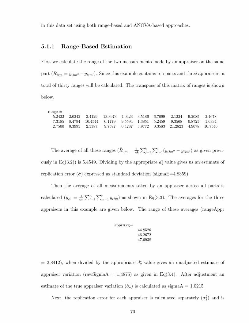
in this data set using both range-based and ANOVA-based approaches.
5.1.1 Range-Based Estimation
First we calculate the range of the two measurements made by an appraiser on the same
part (Rijm = yijm′′−yijm′). Since this example contains ten parts and three appraisers, a
total of thirty ranges will be calculated. The transpose of this matrix of ranges is shown
below.
ranges=5.2422 2.0242 3.4129 13.3973 4.0423 3.5186 6.7699 2.1224 9.2085 2.46787.3185 8.4794 10.4544 0.1779 9.5594 1.3851 5.2459 9.3568 0.8725 1.63342.7500 0.3995 2.3387 9.7597 0.4287 3.9772 0.3583 21.2823 4.9078 10.7546
The average of all these ranges (R..m = 1nk
∑kj=1
∑ni=1(yijm′′ − yijm′) as given previ-
ously in Eq(3.2)) is 5.4549. Dividing by the appropriate d∗2 value gives us an estimate of
replication error (σ) expressed as standard deviation (sigmaE=4.8359).
Then the average of all measurements taken by an appraiser across all parts is
calculated (y.j. = 1nr
∑ni=1
∑rm=1 yijm) as shown in Eq(3.3). The averages for the three
appraisers in this example are given below. The range of these averages (rangeAppr
apprAvg=44.852646.267247.6938
= 2.8412), when divided by the appropriate d∗2 value gives an unadjusted estimate of
appraiser variation (rawSigmaA = 1.4875) as given in Eq(3.4). After adjustment an
estimate of the true appraiser variation (σa) is calculated as sigmaA = 1.0215.
Next, the replication error for each appraiser is calculated separately (σ2j ) and is
70
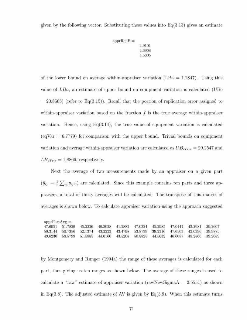
given by the following vector. Substituting these values into Eq(3.13) gives an estimate
apprRepE =4.91014.69684.5005
of the lower bound on average within-appraiser variation (LBa = 1.2847). Using this
value of LBa, an estimate of upper bound on equipment variation is calculated (UBe
= 20.8565) (refer to Eq(3.15)). Recall that the portion of replication error assigned to
within-appraiser variation based on the fraction f is the true average within-appraiser
variation. Hence, using Eq(3.14), the true value of equipment variation is calculated
(eqVar = 6.7779) for comparison with the upper bound. Trivial bounds on equipment
variation and average within-appraiser variation are calculated as UBeTriv = 20.2547 and
LBaTriv = 1.8866, respectively.
Next the average of two measurements made by an appraiser on a given part
(yij. = 1r
∑m yijm) are calculated. Since this example contains ten parts and three ap-
praisers, a total of thirty averages will be calculated. The transpose of this matrix of
averages is shown below. To calculate appraiser variation using the approach suggested
apprPartAvg =47.6951 51.7829 45.2226 40.3028 41.5885 47.0324 45.2985 47.0444 43.2981 39.260750.3144 50.7356 52.1374 43.2223 43.4798 53.8739 39.2316 47.6503 42.0396 39.987549.6230 58.5799 51.5885 44.0160 43.5208 50.8825 44.5632 46.6087 48.2866 39.2689
by Montgomery and Runger (1994a) the range of these averages is calculated for each
part, thus giving us ten ranges as shown below. The average of these ranges is used to
calculate a “raw” estimate of appraiser variation (rawNewSigmaA = 2.5551) as shown
in Eq(3.8). The adjusted estimate of AV is given by Eq(3.9). When this estimate turns
71
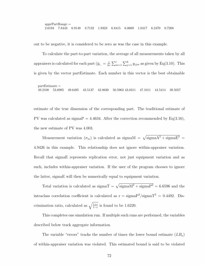
apprPartRange =2.6194 7.8443 6.9148 3.7132 1.9323 6.8415 6.0669 1.0417 6.2470 0.7268
out to be negative, it is considered to be zero as was the case in this example.
To calculate the part-to-part variation, the average of all measurements taken by all
appraisers is calculated for each part (yi.. = 1kr
∑rm=1
∑kj=1 yijm as given by Eq(3.10). This
is given by the vector partEstimate. Each number in this vector is the best obtainable
partEstimate =49.2108 53.6995 49.6495 42.5137 42.8630 50.5963 43.0311 47.1011 44.5414 39.5057
estimate of the true dimension of the corresponding part. The traditional estimate of
PV was calculated as sigmaP = 4.4634. After the correction recommended by Eq(3.16),
the new estimate of PV was 4.003.
Measurement variation (σm) is calculated as sigmaM =√
sigmaA2 + sigmaE2 =
4.9426 in this example. This relationship does not ignore within-appraiser variation.
Recall that sigmaE represents replication error, not just equipment variation and as
such, includes within-appraiser variation. If the user of the program chooses to ignore
the latter, sigmaE will then be numerically equal to equipment variation.
Total variation is calculated as sigmaT =√
sigmaM2 + sigmaP2 = 6.6596 and the
intraclass correlation coefficient is calculated as r = sigmaP2/sigmaT2 = 0.4492. Dis-
crimination ratio, calculated as√
1+r1−r
is found to be 1.6220.
This completes one simulation run. If multiple such runs are performed, the variables
described below track aggregate information.
The variable “errors” tracks the number of times the lower bound estimate (LBa)
of within-appraiser variation was violated. This estimated bound is said to be violated
72

if the true within-appraiser variation is less than LBa. The variables a2a, repE and p2p
calculate the mean of vectors sigmaA, sigmaE, and sigmaP, respectively. They repre-
sent appraiser-to-appraiser, replication error and part-to-part variation averaged over all
simulation runs. The variable mv =√
a2a2 + repE2 calculates the average measurement
variation and tv =√
mv2 + p2p2 calculates the average total variation. Measurement
variation as a percent of total variation expressed as standard deviation is calculated as
percTVsd = mv/tv and the same value expressed as variance is calculated as percTVvar
= percTVsd2.
5.1.2 ANOVA-Based Estimation
Consider the following matrices—part and appr. Each has n = 10 rows and kxr = 3x2 =
6 columns where n, k, and r represent, as usual, number of parts, number of appraisers
and number of replications. For the measurement value in any cell of the “measurement”
part =1 1 1 1 1 12 2 2 2 2 23 3 3 3 3 34 4 4 4 4 45 5 5 5 5 56 6 6 6 6 67 7 7 7 7 78 8 8 8 8 89 9 9 9 9 910 10 10 10 10 10
matrix shown earlier, the corresponding cell in the “part” and “appr” matrices reveals
which part and appraiser the measurement is associated with.
Stacking the columns of each of the three matrices—measurements, part, and appr,
into a single column and then merging the columns together prepares the data for ANOVA
as shown in the table below.
73
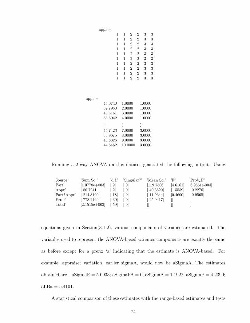
appr =1 1 2 2 3 31 1 2 2 3 31 1 2 2 3 31 1 2 2 3 31 1 2 2 3 31 1 2 2 3 31 1 2 2 3 31 1 2 2 3 31 1 2 2 3 31 1 2 2 3 3
appr =45.0740 1.0000 1.000052.7950 2.0000 1.000043.5161 3.0000 1.000033.6042 4.0000 1.0000...
......
44.7423 7.0000 3.000035.9675 8.0000 3.000045.8326 9.0000 3.000044.6462 10.0000 3.0000
Running a 2-way ANOVA on this dataset generated the following output. Using
’Source’ ’Sum Sq.’ ’d.f.’ ’Singular?’ ’Mean Sq.’ ’F’ ’Prob¿F’’Part’ [1.0778e+003] [ 9] [ 0] [119.7506] [4.6161] [6.9651e-004]’Appr’ [ 80.7241] [ 2] [ 0] [ 40.3620] [1.5559] [ 0.2276]’Part*Appr’ [ 214.8190] [ 18] [ 0] [ 11.9344] [0.4600] [ 0.9565]’Error’ [ 778.2499] [ 30] [ 0] [ 25.9417] [] []’Total’ [2.1515e+003] [ 59] [ 0] [] [] []
equations given in Section(3.1.2), various components of variance are estimated. The
variables used to represent the ANOVA-based variance components are exactly the same
as before except for a prefix ‘a’ indicating that the estimate is ANOVA-based. For
example, appraiser variation, earlier sigmaA, would now be aSigmaA. The estimates
obtained are—aSigmaE = 5.0933; aSigmaPA = 0; aSigmaA = 1.1922; aSigmaP = 4.2390;
aLBa = 5.4101.
A statistical comparison of these estimates with the range-based estimates and tests
74
of effectiveness of the estimates based on multiple simulation runs is shown in the next
section.
5.1.3 Analyzing the Results
Traditionally, range-based estimates are considered inferior to ANOVA-based estimates.
In this section tests will be performed for the hypothesis that the two approaches are
essentially the same. Also, tests will be performed to evaluate whether these estimates are
statistically equal to the true value being estimated and the effectiveness of the estimates
of bounds, LBa and UBe, will be examined.
Comparing ANOVA Estimates with Range-Based Estimates
To compare the estimates obtained using ANOVA with range-based estimates a sample
of size 20 was obtained using 20 consecutive simulation runs using the default set of
parameters—n = 10, k = 3, r = 3, σp = 5, σa = 2, σ = 2, f = 0.5. Remember σ2e =
fσ2. For each statistic to be compared, a paired t-test was performed based on a 95%
confidence using Minitab. The results are displayed in Table(5.1). The hypotheses,
that the ANOVA based estimates of various parameters are equal to their range-based
estimates, could not be rejected in any case. Clearly there is no significant difference
between these estimates.
Effectiveness of Variance Component Estimates
It has already been established that there is no significant difference between ANOVA-
based and range-based estimates of variance components (VCs). Hence, the tests in this
section will be conducted using only the range-based estimates. To test whether the VC
75
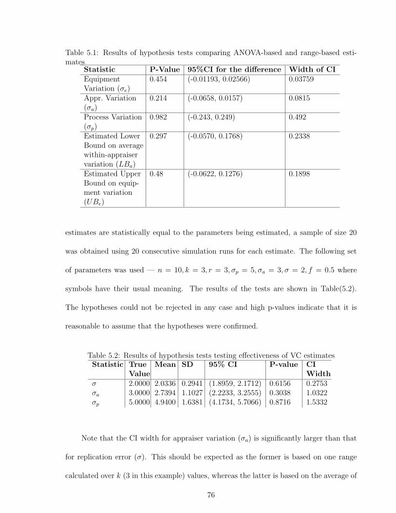
Table 5.1: Results of hypothesis tests comparing ANOVA-based and range-based esti-mates
Statistic P-Value 95%CI for the difference Width of CIEquipmentVariation (σe)
0.454 (-0.01193, 0.02566) 0.03759
Appr. Variation(σa)
0.214 (-0.0658, 0.0157) 0.0815
Process Variation(σp)
0.982 (-0.243, 0.249) 0.492
Estimated LowerBound on averagewithin-appraiservariation (LBa)
0.297 (-0.0570, 0.1768) 0.2338
Estimated UpperBound on equip-ment variation(UBe)
0.48 (-0.0622, 0.1276) 0.1898
estimates are statistically equal to the parameters being estimated, a sample of size 20
was obtained using 20 consecutive simulation runs for each estimate. The following set
of parameters was used — n = 10, k = 3, r = 3, σp = 5, σa = 3, σ = 2, f = 0.5 where
symbols have their usual meaning. The results of the tests are shown in Table(5.2).
The hypotheses could not be rejected in any case and high p-values indicate that it is
reasonable to assume that the hypotheses were confirmed.
Table 5.2: Results of hypothesis tests testing effectiveness of VC estimatesStatistic True
ValueMean SD 95% CI P-value CI
Widthσ 2.0000 2.0336 0.2941 (1.8959, 2.1712) 0.6156 0.2753σa 3.0000 2.7394 1.1027 (2.2233, 3.2555) 0.3038 1.0322σp 5.0000 4.9400 1.6381 (4.1734, 5.7066) 0.8716 1.5332
Note that the CI width for appraiser variation (σa) is significantly larger than that
for replication error (σ). This should be expected as the former is based on one range
calculated over k (3 in this example) values, whereas the latter is based on the average of
76
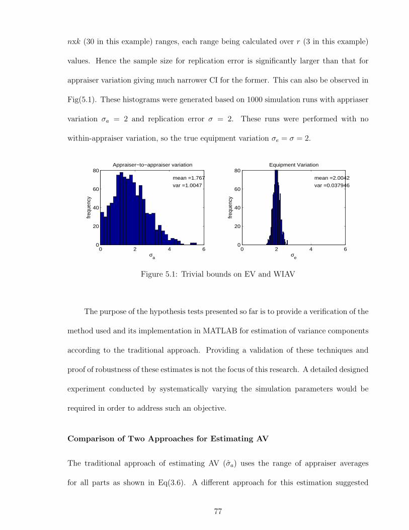
nxk (30 in this example) ranges, each range being calculated over r (3 in this example)
values. Hence the sample size for replication error is significantly larger than that for
appraiser variation giving much narrower CI for the former. This can also be observed in
Fig(5.1). These histograms were generated based on 1000 simulation runs with appriaser
variation σa = 2 and replication error σ = 2. These runs were performed with no
within-appraiser variation, so the true equipment variation σe = σ = 2.
0 2 4 60
20
40
60
80
σa
frequ
ency
Appraiser−to−appraiser variation
mean =1.767
var =1.0047
0 2 4 60
20
40
60
80
σe
frequ
ency
Equipment Variation
mean =2.0042
var =0.037946
Figure 5.1: Trivial bounds on EV and WIAV
The purpose of the hypothesis tests presented so far is to provide a verification of the
method used and its implementation in MATLAB for estimation of variance components
according to the traditional approach. Providing a validation of these techniques and
proof of robustness of these estimates is not the focus of this research. A detailed designed
experiment conducted by systematically varying the simulation parameters would be
required in order to address such an objective.
Comparison of Two Approaches for Estimating AV
The traditional approach of estimating AV (σa) uses the range of appraiser averages
for all parts as shown in Eq(3.6). A different approach for this estimation suggested
77
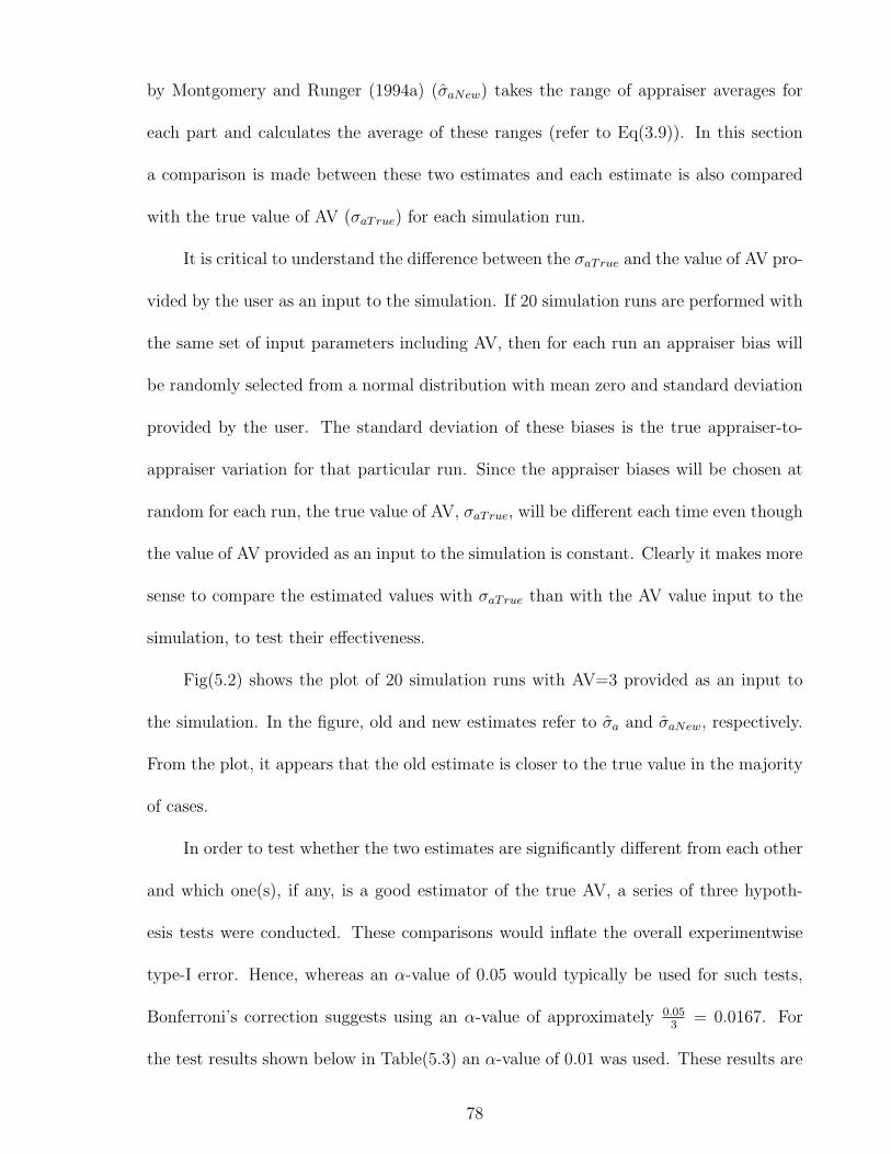
by Montgomery and Runger (1994a) (σaNew) takes the range of appraiser averages for
each part and calculates the average of these ranges (refer to Eq(3.9)). In this section
a comparison is made between these two estimates and each estimate is also compared
with the true value of AV (σaTrue) for each simulation run.
It is critical to understand the difference between the σaTrue and the value of AV pro-
vided by the user as an input to the simulation. If 20 simulation runs are performed with
the same set of input parameters including AV, then for each run an appraiser bias will
be randomly selected from a normal distribution with mean zero and standard deviation
provided by the user. The standard deviation of these biases is the true appraiser-to-
appraiser variation for that particular run. Since the appraiser biases will be chosen at
random for each run, the true value of AV, σaTrue, will be different each time even though
the value of AV provided as an input to the simulation is constant. Clearly it makes more
sense to compare the estimated values with σaTrue than with the AV value input to the
simulation, to test their effectiveness.
Fig(5.2) shows the plot of 20 simulation runs with AV=3 provided as an input to
the simulation. In the figure, old and new estimates refer to σa and σaNew, respectively.
From the plot, it appears that the old estimate is closer to the true value in the majority
of cases.
In order to test whether the two estimates are significantly different from each other
and which one(s), if any, is a good estimator of the true AV, a series of three hypoth-
esis tests were conducted. These comparisons would inflate the overall experimentwise
type-I error. Hence, whereas an α-value of 0.05 would typically be used for such tests,
Bonferroni’s correction suggests using an α-value of approximately 0.053
= 0.0167. For
the test results shown below in Table(5.3) an α-value of 0.01 was used. These results are
78
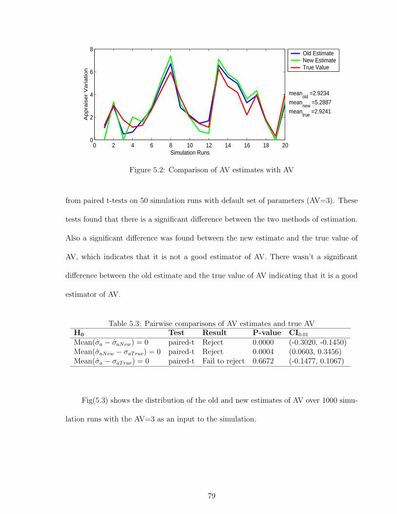
0 2 4 6 8 10 12 14 16 18 200
2
4
6
8
Simulation Runs
Ap
pra
ise
r V
aria
tion
meanold
=2.9234
meannew
=5.2887
meantrue
=2.9241
Old EstimateNew EstimateTrue Value
Figure 5.2: Comparison of AV estimates with AV
from paired t-tests on 50 simulation runs with default set of parameters (AV=3). These
tests found that there is a significant difference between the two methods of estimation.
Also a significant difference was found between the new estimate and the true value of
AV, which indicates that it is not a good estimator of AV. There wasn’t a significant
difference between the old estimate and the true value of AV indicating that it is a good
estimator of AV.
Table 5.3: Pairwise comparisons of AV estimates and true AVH0 Test Result P-value CI0.01
Mean(σa − σaNew) = 0 paired-t Reject 0.0000 (-0.3020, -0.1450)Mean(σaNew − σaTrue) = 0 paired-t Reject 0.0004 (0.0603, 0.3456)Mean(σa − σaTrue) = 0 paired-t Fail to reject 0.6672 (-0.1477, 0.1067)
Fig(5.3) shows the distribution of the old and new estimates of AV over 1000 simu-
lation runs with the AV=3 as an input to the simulation.
79
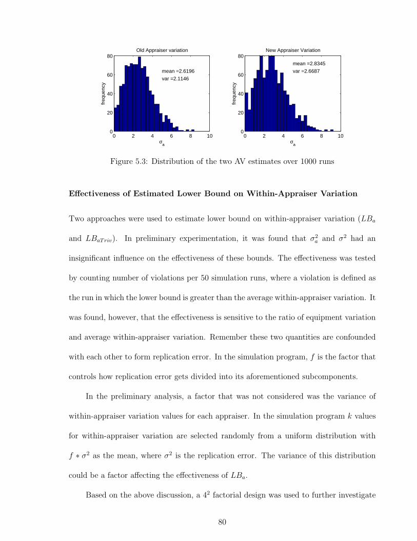
0 2 4 6 8 100
20
40
60
80
σa
freq
uenc
y
Old Appraiser variation
mean =2.6196
var =2.1146
0 2 4 6 8 100
20
40
60
80
σa
freq
uenc
y
New Appraiser Variation
mean =2.8345
var =2.6687
Figure 5.3: Distribution of the two AV estimates over 1000 runs
Effectiveness of Estimated Lower Bound on Within-Appraiser Variation
Two approaches were used to estimate lower bound on within-appraiser variation (LBa
and LBaTriv). In preliminary experimentation, it was found that σ2a and σ2 had an
insignificant influence on the effectiveness of these bounds. The effectiveness was tested
by counting number of violations per 50 simulation runs, where a violation is defined as
the run in which the lower bound is greater than the average within-appraiser variation. It
was found, however, that the effectiveness is sensitive to the ratio of equipment variation
and average within-appraiser variation. Remember these two quantities are confounded
with each other to form replication error. In the simulation program, f is the factor that
controls how replication error gets divided into its aforementioned subcomponents.
In the preliminary analysis, a factor that was not considered was the variance of
within-appraiser variation values for each appraiser. In the simulation program k values
for within-appraiser variation are selected randomly from a uniform distribution with
f ∗ σ2 as the mean, where σ2 is the replication error. The variance of this distribution
could be a factor affecting the effectiveness of LBa.
Based on the above discussion, a 42 factorial design was used to further investigate
80

the effectiveness of LBa. The two factors were the fraction f and the variance of the
uniform distribution from which the actual within-appraiser variation values are selected,
say V . The factor levels are shown in Table(5.4). The extreme values for f , 0.0 and 1.0,
were deliberately avoided under the premise that it is impossible to completely eliminate
the effect of either within-appraiser variation or EV from an experiment.
Table 5.4: Factor levels for testing the effectiveness of within-appraiser variationFactor Symbol Levelsf 0.2, 0.4, 0.6, 0.8
V 12
12, 1.52
12, 22
12, 2.52
12
The response variable for this experiment (Y ) was number of “violations” observed
in 50 simulation runs for each of the estimated bounds—LBa, LBaTriv, UBe, and UBeTriv.
The values of Y for each of 16 treatment combinations are shown in Table(D.1) in
Appendix(D). The analysis of each response variable revealed that the interaction be-
tween f and V is not significant. Further analysis showed (see Appendix (E)) that the
variance, V , is marginally significant in two cases (LBa, UBeTriv) and not at all sig-
nificant in the remaining two. However, f was highly significant in affecting all four
response variables. A box plot of each response variable with respect to variation in
f (see Fig(5.4)) shows that the response decreases with an increase in f . This indi-
cates that as the proportion of within-appraiser variation increases in the replication
error, the estimates of bounds become more effective. Fig(5.5) and Fig(5.6) show the
results of the two types of bound estimates over 20 simulation runs for the parameter
set—n = 10, k = 3, r = 3, σp = 6, σa = 3, σ = 2, f = 0.8, V = 1.
From Fig(5.5) it is evident that in the traditional estimate of EV significantly over-
estimates equipment variation. The upper bound (UBe), in such cases, can provide a
81
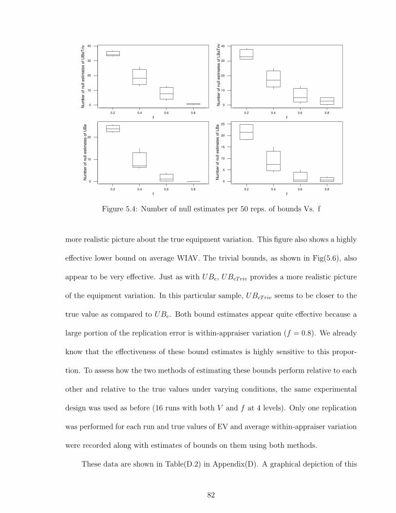
0.80.60.40.2
40
30
20
10
0
f
Num
ber
of null e
stim
ate
s o
f U
BeT
riv
0.80.60.40.2
40
30
20
10
0
f
Num
ber
of null e
stim
ate
s o
f LB
aT
riv
0.80.60.40.2
20
10
0
f
Num
ber
of
null e
stim
ate
s o
f U
Be
0.80.60.40.2
25
20
15
10
5
0
f
Num
ber
of
null e
stim
ate
s o
f LB
a
Figure 5.4: Number of null estimates per 50 reps. of bounds Vs. f
more realistic picture about the true equipment variation. This figure also shows a highly
effective lower bound on average WIAV. The trivial bounds, as shown in Fig(5.6), also
appear to be very effective. Just as with UBe, UBeTriv provides a more realistic picture
of the equipment variation. In this particular sample, UBeTriv seems to be closer to the
true value as compared to UBe. Both bound estimates appear quite effective because a
large portion of the replication error is within-appraiser variation (f = 0.8). We already
know that the effectiveness of these bound estimates is highly sensitive to this propor-
tion. To assess how the two methods of estimating these bounds perform relative to each
other and relative to the true values under varying conditions, the same experimental
design was used as before (16 runs with both V and f at 4 levels). Only one replication
was performed for each run and true values of EV and average within-appraiser variation
were recorded along with estimates of bounds on them using both methods.
These data are shown in Table(D.2) in Appendix(D). A graphical depiction of this
82
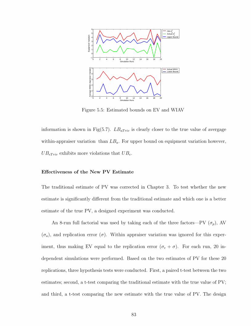
0 2 4 6 8 10 12 14 16 18 20−1
0
1
2
3
4
5
6
Simulation Runs
Equ
ipm
ent V
aria
tion
Old σe2
Actual σe2
Upper Bound
0 2 4 6 8 10 12 14 16 18 200
1
2
3
4
5
Simulation Runs
Ave
rage
With
in A
ppra
iser
Var
iatio
n
Actual WIAVLower Bound
Figure 5.5: Estimated bounds on EV and WIAV
information is shown in Fig(5.7). LBaTriv is clearly closer to the true value of avergage
within-appraiser variation than LBa. For upper bound on equipment variation however,
UBeTriv exhibits more violations that UBe.
Effectiveness of the New PV Estimate
The traditional estimate of PV was corrected in Chapter 3. To test whether the new
estimate is significantly different from the traditional estimate and which one is a better
estimate of the true PV, a designed experiment was conducted.
An 8-run full factorial was used by taking each of the three factors—PV (σp), AV
(σa), and replication error (σ). Within appraiser variation was ignored for this exper-
iment, thus making EV equal to the replication error (σe + σ). For each run, 20 in-
dependent simulations were performed. Based on the two estimates of PV for these 20
replications, three hypothesis tests were conducted. First, a paired t-test between the two
estimates; second, a t-test comparing the traditional estimate with the true value of PV;
and third, a t-test comparing the new estimate with the true value of PV. The design
83
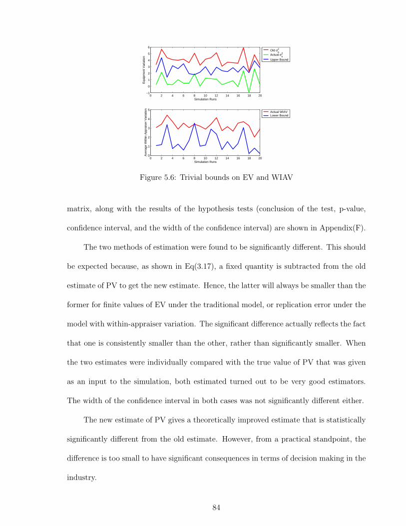
0 2 4 6 8 10 12 14 16 18 20−1
0
1
2
3
4
5
6
Simulation Runs
Equ
ipm
ent V
aria
tion
Old σe2
Actual σe2
Upper Bound
0 2 4 6 8 10 12 14 16 18 200
1
2
3
4
5
Simulation Runs
Ave
rage
With
in A
ppra
iser
Var
iatio
n
Actual WIAVLower Bound
Figure 5.6: Trivial bounds on EV and WIAV
matrix, along with the results of the hypothesis tests (conclusion of the test, p-value,
confidence interval, and the width of the confidence interval) are shown in Appendix(F).
The two methods of estimation were found to be significantly different. This should
be expected because, as shown in Eq(3.17), a fixed quantity is subtracted from the old
estimate of PV to get the new estimate. Hence, the latter will always be smaller than the
former for finite values of EV under the traditional model, or replication error under the
model with within-appraiser variation. The significant difference actually reflects the fact
that one is consistently smaller than the other, rather than significantly smaller. When
the two estimates were individually compared with the true value of PV that was given
as an input to the simulation, both estimated turned out to be very good estimators.
The width of the confidence interval in both cases was not significantly different either.
The new estimate of PV gives a theoretically improved estimate that is statistically
significantly different from the old estimate. However, from a practical standpoint, the
difference is too small to have significant consequences in terms of decision making in the
industry.
84
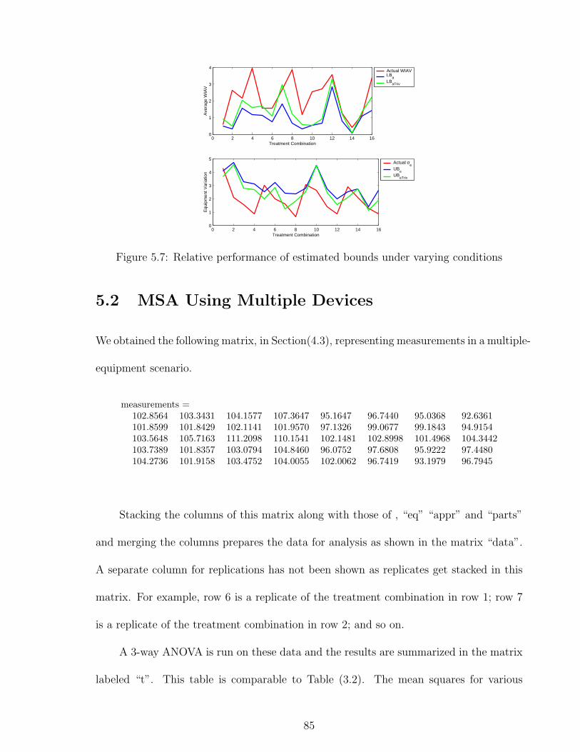
0 2 4 6 8 10 12 14 160
1
2
3
4
Treatment Combination
Ave
rage
WIA
V
Actual WIAVLB
aLB
aTriv
0 2 4 6 8 10 12 14 160
1
2
3
4
5
Treatment Combination
Equ
ipm
ent V
aria
tion
Actual σe
UBe
UBeTriv
Figure 5.7: Relative performance of estimated bounds under varying conditions
5.2 MSA Using Multiple Devices
We obtained the following matrix, in Section(4.3), representing measurements in a multiple-
equipment scenario.
measurements =102.8564 103.3431 104.1577 107.3647 95.1647 96.7440 95.0368 92.6361101.8599 101.8429 102.1141 101.9570 97.1326 99.0677 99.1843 94.9154103.5648 105.7163 111.2098 110.1541 102.1481 102.8998 101.4968 104.3442103.7389 101.8357 103.0794 104.8460 96.0752 97.6808 95.9222 97.4480104.2736 101.9158 103.4752 104.0055 102.0062 96.7419 93.1979 96.7945
Stacking the columns of this matrix along with those of , “eq” “appr” and “parts”
and merging the columns prepares the data for analysis as shown in the matrix “data”.
A separate column for replications has not been shown as replicates get stacked in this
matrix. For example, row 6 is a replicate of the treatment combination in row 1; row 7
is a replicate of the treatment combination in row 2; and so on.
A 3-way ANOVA is run on these data and the results are summarized in the matrix
labeled “t”. This table is comparable to Table (3.2). The mean squares for various
85
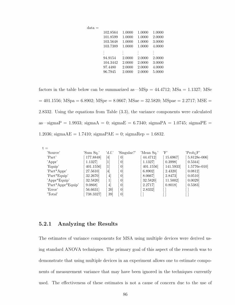
data =102.8564 1.0000 1.0000 1.0000101.8599 1.0000 1.0000 2.0000103.5648 1.0000 1.0000 3.0000103.7389 1.0000 1.0000 4.0000...
......
...94.9154 2.0000 2.0000 2.0000104.3442 2.0000 2.0000 3.000097.4480 2.0000 2.0000 4.000096.7945 2.0000 2.0000 5.0000
factors in the table below can be summarized as—MSp = 44.4712; MSa = 1.1327; MSe
= 401.1556; MSpa = 6.8902; MSpe = 8.0667; MSae = 32.5820; MSpae = 2.2717; MSE =
2.8332. Using the equations from Table (3.3), the variance components were calculated
as—sigmaP = 1.9933; sigmaA = 0; sigmaE = 6.7340; sigmaPA = 1.0745; sigmaPE =
1.2036; sigmaAE = 1.7410; sigmaPAE = 0; sigmaRep = 1.6832.
t =’Source’ ’Sum Sq.’ ’d.f.’ ’Singular?’ ’Mean Sq.’ ’F’ ’Prob¿F’’Part’ [ 177.8848] [4] [ 0] [ 44.4712] [ 15.6967] [ 5.8128e-006]’Appr’ [ 1.1327] [1] [ 0] [ 1.1327] [ 0.3998] [ 0.5344]’Equip’ [ 401.1556] [1] [ 0] [ 401.1556] [ 141.5933] [ 1.5776e-010]’Part*Appr’ [ 27.5610] [4] [ 0] [ 6.8902] [ 2.4320] [ 0.0812]’Part*Equip’ [ 32.2670] [ 4] [ 0] [ 8.0667] [ 2.8473] [ 0.0510]’Appr*Equip’ [ 32.5820] [ 1] [ 0] [ 32.5820] [ 11.5002] [ 0.0029]’Part*Appr*Equip’ [ 9.0868] [ 4] [ 0] [ 2.2717] [ 0.8018] [ 0.5383]’Error’ [ 56.6631] [ 20] [ 0] [ 2.8332] [ ] [ ]’Total’ [ 738.3327] [ 39] [ 0] [ ] [ ] [ ]
5.2.1 Analyzing the Results
The estimates of variance components for MSA using multiple devices were derived us-
ing standard ANOVA techniques. The primary goal of this aspect of the research was to
demonstrate that using multiple devices in an experiment allows one to estimate compo-
nents of measurement variance that may have been ignored in the techniques currently
used. The effectiveness of these estimates is not a cause of concern due to the use of
86
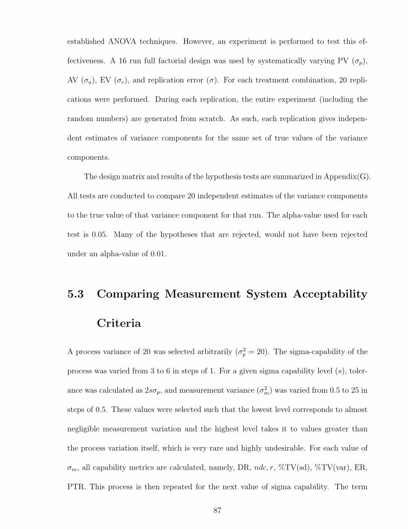
established ANOVA techniques. However, an experiment is performed to test this ef-
fectiveness. A 16 run full factorial design was used by systematically varying PV (σp),
AV (σa), EV (σe), and replication error (σ). For each treatment combination, 20 repli-
cations were performed. During each replication, the entire experiment (including the
random numbers) are generated from scratch. As such, each replication gives indepen-
dent estimates of variance components for the same set of true values of the variance
components.
The design matrix and results of the hypothesis tests are summarized in Appendix(G).
All tests are conducted to compare 20 independent estimates of the variance components
to the true value of that variance component for that run. The alpha-value used for each
test is 0.05. Many of the hypotheses that are rejected, would not have been rejected
under an alpha-value of 0.01.
5.3 Comparing Measurement System Acceptability
Criteria
A process variance of 20 was selected arbitrarily (σ2p = 20). The sigma-capability of the
process was varied from 3 to 6 in steps of 1. For a given sigma capability level (s), toler-
ance was calculated as 2sσp, and measurement variance (σ2m) was varied from 0.5 to 25 in
steps of 0.5. These values were selected such that the lowest level corresponds to almost
negligible measurement variation and the highest level takes it to values greater than
the process variation itself, which is very rare and highly undesirable. For each value of
σm, all capability metrics are calculated, namely, DR, ndc, r, %TV(sd), %TV(var), ER,
PTR. This process is then repeated for the next value of sigma capability. The term
87

%TV (sd) is measurement variation as a percent of total variation calculated using stan-
dard deviations, and %TV(var) represents the same quantity calculated using variances.
Table(5.3) shows selected results from this experiment.
Table 5.5: Relative performance of capability metricsSigmaCapability
DR ndc r %TV(sd) %TV(var) ER PTR
3 2.9 3.1 0.82 43% 18% 1.42 40.71%3 5 5.1 0.93 27% 7% 0.85 24.28%3 12.1 12.2 0.98 12% 1% 0.35 10.00%4 2.8 3 0.8 45% 20% 1.5 32.19%4 5 5.1 0.93 27% 7% 0.85 18.21%4 9.1 9.2 0.98 15% 2% 0.47 10.00%5 2.9 3.1 0.82 43% 18% 1.43 24.43%5 5 5.1 0.93 27% 7% 0.85 14.57%5 7.3 7.4 0.96 19% 4% 0.58 10.00%6 3 3.1 0.82 43% 18% 1.42 20.36%6 5 5.1 0.93 27% 7% 0.85 12.14%6 6 6.1 0.95 23% 5% 0.7 10.00%
Recall that AIAG had increased the recommended value for ndc from 3 to 5 over
time and the generally accepted threshold for PTR is 10%. Hence, for each level of sigma
capability, three records have been displayed. The first two correspond to an ndc of 3
and 5 respectively and the third corresponds to a PTR of 10%.
For metrics like DR, ndc, and r higher values are desirable, whereas for %TV and
PTR lower values are desirable. As the sigma capability of the process increases, PTR
reduces for a given DR. This should be expected because as the sigma capability of
a process increases, either the process variance decreases or tolerance increases. It is
interesting to note that when DR and ndc are close to 3, PTR is extremely high regardless
of the sigma quality. For DR close to 5, it is relatively low but still at unacceptable levels
regardless of sigma capability. This means that the same measurement system may be
88
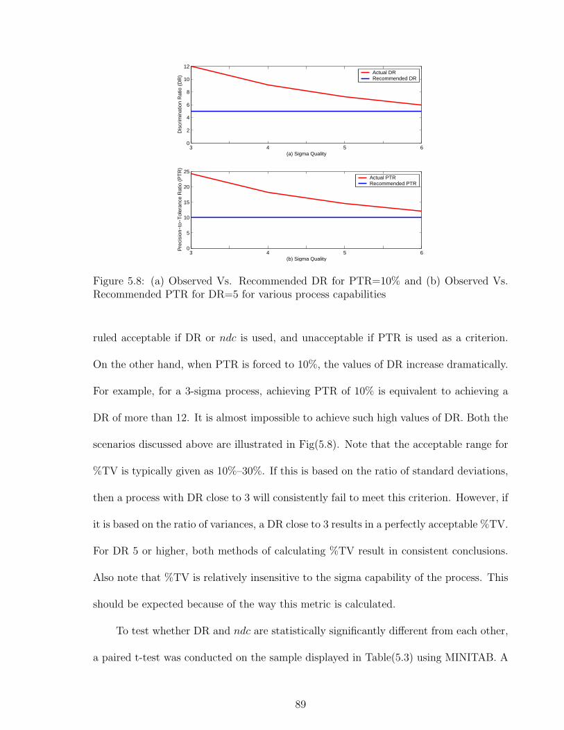
3 4 5 60
2
4
6
8
10
12
(a) Sigma Quality
Dis
crim
inat
ion
Rat
io (
DR
) Actual DRRecommended DR
3 4 5 60
5
10
15
20
25
(b) Sigma Quality
Pre
cisi
on−
to−
Tol
eran
ce R
atio
(P
TR
)Actual PTRRecommended PTR
Figure 5.8: (a) Observed Vs. Recommended DR for PTR=10% and (b) Observed Vs.Recommended PTR for DR=5 for various process capabilities
ruled acceptable if DR or ndc is used, and unacceptable if PTR is used as a criterion.
On the other hand, when PTR is forced to 10%, the values of DR increase dramatically.
For example, for a 3-sigma process, achieving PTR of 10% is equivalent to achieving a
DR of more than 12. It is almost impossible to achieve such high values of DR. Both the
scenarios discussed above are illustrated in Fig(5.8). Note that the acceptable range for
%TV is typically given as 10%–30%. If this is based on the ratio of standard deviations,
then a process with DR close to 3 will consistently fail to meet this criterion. However, if
it is based on the ratio of variances, a DR close to 3 results in a perfectly acceptable %TV.
For DR 5 or higher, both methods of calculating %TV result in consistent conclusions.
Also note that %TV is relatively insensitive to the sigma capability of the process. This
should be expected because of the way this metric is calculated.
To test whether DR and ndc are statistically significantly different from each other,
a paired t-test was conducted on the sample displayed in Table(5.3) using MINITAB. A
89
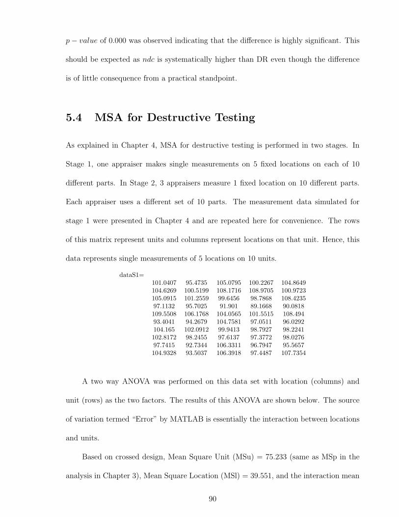
p− value of 0.000 was observed indicating that the difference is highly significant. This
should be expected as ndc is systematically higher than DR even though the difference
is of little consequence from a practical standpoint.
5.4 MSA for Destructive Testing
As explained in Chapter 4, MSA for destructive testing is performed in two stages. In
Stage 1, one appraiser makes single measurements on 5 fixed locations on each of 10
different parts. In Stage 2, 3 appraisers measure 1 fixed location on 10 different parts.
Each appraiser uses a different set of 10 parts. The measurement data simulated for
stage 1 were presented in Chapter 4 and are repeated here for convenience. The rows
of this matrix represent units and columns represent locations on that unit. Hence, this
data represents single measurements of 5 locations on 10 units.
dataS1=101.0407 95.4735 105.0795 100.2267 104.8649104.6269 100.5199 108.1716 108.9705 100.9723105.0915 101.2559 99.6456 98.7868 108.423597.1132 95.7025 91.901 89.1668 90.0818109.5508 106.1768 104.0565 101.5515 108.49493.4041 94.2679 104.7581 97.0511 96.0292104.165 102.0912 99.9413 98.7927 98.2241102.8172 98.2455 97.6137 97.3772 98.027697.7415 92.7344 106.3311 96.7947 95.5657104.9328 93.5037 106.3918 97.4487 107.7354
A two way ANOVA was performed on this data set with location (columns) and
unit (rows) as the two factors. The results of this ANOVA are shown below. The source
of variation termed “Error” by MATLAB is essentially the interaction between locations
and units.
Based on crossed design, Mean Square Unit (MSu) = 75.233 (same as MSp in the
analysis in Chapter 3), Mean Square Location (MSl) = 39.551, and the interaction mean
90
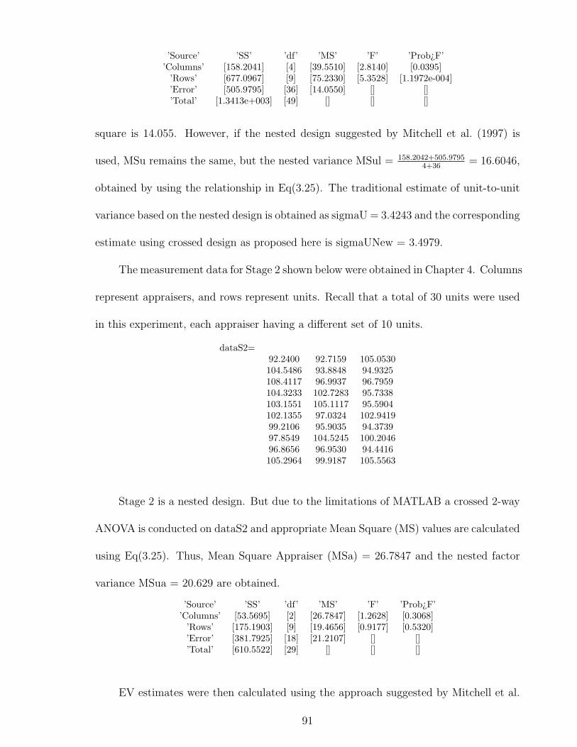
’Source’ ’SS’ ’df’ ’MS’ ’F’ ’Prob¿F’’Columns’ [158.2041] [4] [39.5510] [2.8140] [0.0395]
’Rows’ [677.0967] [9] [75.2330] [5.3528] [1.1972e-004]’Error’ [505.9795] [36] [14.0550] [] []’Total’ [1.3413e+003] [49] [] [] []
square is 14.055. However, if the nested design suggested by Mitchell et al. (1997) is
used, MSu remains the same, but the nested variance MSul = 158.2042+505.97954+36
= 16.6046,
obtained by using the relationship in Eq(3.25). The traditional estimate of unit-to-unit
variance based on the nested design is obtained as sigmaU = 3.4243 and the corresponding
estimate using crossed design as proposed here is sigmaUNew = 3.4979.
The measurement data for Stage 2 shown below were obtained in Chapter 4. Columns
represent appraisers, and rows represent units. Recall that a total of 30 units were used
in this experiment, each appraiser having a different set of 10 units.
dataS2=92.2400 92.7159 105.0530104.5486 93.8848 94.9325108.4117 96.9937 96.7959104.3233 102.7283 95.7338103.1551 105.1117 95.5904102.1355 97.0324 102.941999.2106 95.9035 94.373997.8549 104.5245 100.204696.8656 96.9530 94.4416105.2964 99.9187 105.5563
Stage 2 is a nested design. But due to the limitations of MATLAB a crossed 2-way
ANOVA is conducted on dataS2 and appropriate Mean Square (MS) values are calculated
using Eq(3.25). Thus, Mean Square Appraiser (MSa) = 26.7847 and the nested factor
variance MSua = 20.629 are obtained.
’Source’ ’SS’ ’df’ ’MS’ ’F’ ’Prob¿F’’Columns’ [53.5695] [2] [26.7847] [1.2628] [0.3068]
’Rows’ [175.1903] [9] [19.4656] [0.9177] [0.5320]’Error’ [381.7925] [18] [21.2107] [] []’Total’ [610.5522] [29] [] [] []
EV estimates were then calculated using the approach suggested by Mitchell et al.
91
(1997) (sigmaE = 2.9838) and the improved approach suggested here (sigmaEnew =
2.8971). The estimate of AV (sigmaA) was the same for both the approaches and was
found to be 0.7846.
5.4.1 Analyzing the Results
The objectives of this analysis are—to test if the VC estimation approach given by
Mitchell et al. (1997) produces reliable estimates; to test if the improved approach sug-
gested in this research is significantly different; and to test whether the improved approach
produces reliable estimates. To test these hypotheses a designed experiment is conducted
by systematically varying potentially influential factors and conducting the analysis in
the form of appropriate statistical tests.
The factors that could potentially affect the estimate of EV (σe) and AV (σa) are
the true values of EV (σe), AV (σa), UV (σu), LV(σl), and the interaction between unit
and location (σul). A Central Composite Design (CCD) was chosen for this analysis.
The specific form was chosen from MINITAB with standard axials and 10 center points
creating a total of 52 treatment combinations (TCs). The details of the factors and
levels used are shown in the Appendix(I) in the form of a design matrix. For each TC, 50
replications were performed and statistics were collected. Each replication was conducted
as an independent analysis such that all random numbers were generated from scratch
for each replication. To conduct this experiment a design matrix of input parameters
was created in Microsoft Excel. This spreadsheet was read by a program (in MATLAB)
which in turn invoked another program performing the MSAD analysis for each TC in
the design. It performed 50 replications, conducted the appropriate hypothesis tests and
published the results of these tests to a text file. The design matrix along with the test
92
results can be found in Appendix(I).
The unit mean (µ) was 100 for this experiment. The high and low (1 and -1) for σe,
σa, σu, and σl were 3 and 7 respectively and the centerpoint was 5. Coded axial value of
α = n1/4f = 2.3784 was used for these factors, which is equivalent to 0.24317 and 9.75683
in terms of true factor settings. In the previous expression, nf is the number of TCs in
the factorial portion of the experiment. For σul, the high and low values were 2 and 4
respectively, yielding axial values of 0.62159 and 5.37841.
H0 : The two methods of estimating σe are statistically equivalent
The first hypothesis to be tested is regarding the difference between the two approaches
for estimating EV—the one provided by Mitchell et al. (1997) (σe) and the one suggested
as a part of this research (σeNew). A paired t-test was conducted on σe and σeNew using
50 replications for each of the 52 TCs in the experiment. A 99% CI was used to make
the test even more stringent. The hypothesis that the two methods are equivalent was
rejected 51 out of the 52 times. The TC for which this hypothesis was not rejected was
when σa was set to its −α and all other factors were at center points. Clearly there is
a significant difference between the two approaches. The new EV estimate (σeNew) was
consistently and significantly lower than the old estimate, σe.
H0 : σe is a good estimator of σe
The hypothesis tested above merely suggests that the two methods are different, but
does not indicate if either produces a good estimate of σe. Hence a t-test was conducted
with α = 0.05 for each TC comparing the average of σe (¯σe)with σe. As a result 19 of
the 52 tests were rejected concluding with 95% confidence that this approach was not
93
very effective in estimating σe in these 19 cases. A logistic regression of the result of the
hypothesis test (0 or 1) on the factors of the experiment could provide some insight into
the factors affecting the effectiveness of the estimate. However, a binary response cannot
provide information about the degree of this effect. In other words, any information
about the degree of deviation from the true value will be lost.
Hence the difference between ¯σe for each TC and the corresponding true value, σe,
was calculated as ∆e = σe − ¯σe and an ANOVA / regression was performed with this as
the response variable. All two-way interactions were included in the model but square
terms were left out. The results are displayed in Appendix(J). The regression was highly
significant with R2 = 97.2% and Adj.R2 = 96%. Interaction terms were not significant.
Among the main effects, σu, σl, and σe were the only significant terms. The coefficients
for these factors indicate the kind of effect they have on the error. Remember, ∆e
represents error and not absolute error. Hence factors with negative coefficients should
not be construed as factors that reduce error because error could be negative. The mean
of ∆e over all TCs was -0.2773 and the standard deviation was 2.5281. The mean of
absolute deviations, |∆e|, was 1.7736, which is of much more interest because negative
deviations from the true value are just as undesirable as positive deviations. The average
width of CI on ¯σe was found to be 1.1956.
However, it was found that during many replications the equipment variance, σ2e ,
turns out to be negative and hence the estimate of σe becomes a complex number which
is unacceptable. Under such circumstances σe is considered to be zero. For example,
out of the 50 replications for the the first TC in the experiment, 4 estimates were zero
and for the second TC 12 were zero or null. On average, 4.8654 (9.7%) estimates out
of 50 for each TC were null. These null estimates clearly bias ¯σe for each TC. Hence,
94

a separate analysis was performed after removing all instances where the σe = 0. This
trimmed-mean of estimates, ¯σeTrim, is shown in Table(I.4).
A hypothesis test was performed again for each TC with this new mean. In this
case 30 out of 52 tests were rejected. It appears as if the null estimates were lowering
the mean estimate bringing it closer to the true value. As before, ANOVA / regression
was performed with ∆eTrim = σe − ¯σeTrim as the response variable. The results were
very similar to those obtained earlier— σu, σl, and σe were the only significant terms;
the coefficients have the same sign as before; and the R2 and Adj. R2 values were very
similar to the previous analysis. These results are not shown. The average of ∆eTrim
was found to be -0.78777 and the standard deviation was 2.1144. Again, since absolute
deviations are of more interest the mean of |∆eTrim| was calculated as 1.5810. The width
of CI on ¯σeTrim was found to be 0.9897.
The mean absolute deviation was less for the trimmed mean and the width of the
CI also decreased significantly. However, since the mean of the raw deviations has moved
farther away from zero, the hypothesis is rejected in a significantly larger number of
cases when the trimmed mean was used. In practice, since the cases in which a variance
estimate turns out to be negative are typically discarded, the analysis with trimmed
mean is more relevant.
H0 : σeNew is a good estimator of σe
The analysis presented in this section is very similar to the one in the previous section.
Only, in this section it is being performed on the improved estimate of σe suggested as a
part of this research, σeNew.
A t-test was conducted with α = 0.05 for each TC comparing the average of σeNew
95
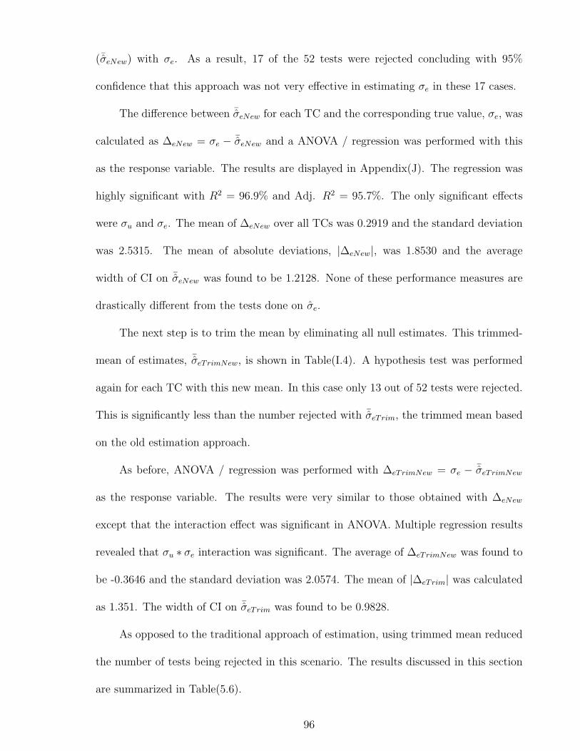
(¯σeNew) with σe. As a result, 17 of the 52 tests were rejected concluding with 95%
confidence that this approach was not very effective in estimating σe in these 17 cases.
The difference between ¯σeNew for each TC and the corresponding true value, σe, was
calculated as ∆eNew = σe − ¯σeNew and a ANOVA / regression was performed with this
as the response variable. The results are displayed in Appendix(J). The regression was
highly significant with R2 = 96.9% and Adj. R2 = 95.7%. The only significant effects
were σu and σe. The mean of ∆eNew over all TCs was 0.2919 and the standard deviation
was 2.5315. The mean of absolute deviations, |∆eNew|, was 1.8530 and the average
width of CI on ¯σeNew was found to be 1.2128. None of these performance measures are
drastically different from the tests done on σe.
The next step is to trim the mean by eliminating all null estimates. This trimmed-
mean of estimates, ¯σeTrimNew, is shown in Table(I.4). A hypothesis test was performed
again for each TC with this new mean. In this case only 13 out of 52 tests were rejected.
This is significantly less than the number rejected with ¯σeTrim, the trimmed mean based
on the old estimation approach.
As before, ANOVA / regression was performed with ∆eTrimNew = σe − ¯σeTrimNew
as the response variable. The results were very similar to those obtained with ∆eNew
except that the interaction effect was significant in ANOVA. Multiple regression results
revealed that σu ∗ σe interaction was significant. The average of ∆eTrimNew was found to
be -0.3646 and the standard deviation was 2.0574. The mean of |∆eTrim| was calculated
as 1.351. The width of CI on ¯σeTrim was found to be 0.9828.
As opposed to the traditional approach of estimation, using trimmed mean reduced
the number of tests being rejected in this scenario. The results discussed in this section
are summarized in Table(5.6).
96
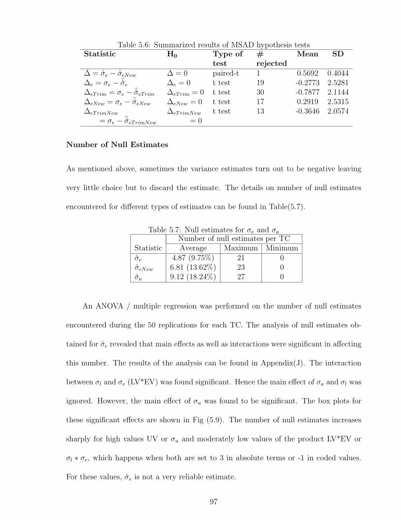
Table 5.6: Summarized results of MSAD hypothesis testsStatistic H0 Type of
test#rejected
Mean SD
∆ = σe − σeNew ∆ = 0 paired-t 1 0.5692 0.4044∆e = σe − ¯σe ∆e = 0 t test 19 -0.2773 2.5281∆eTrim = σe − ¯σeTrim ∆eTrim = 0 t test 30 -0.7877 2.1144∆eNew = σe − ¯σeNew ∆eNew = 0 t test 17 0.2919 2.5315∆eTrimNew
= σe − ¯σeTrimNew
∆eTrimNew
= 0t test 13 -0.3646 2.0574
Number of Null Estimates
As mentioned above, sometimes the variance estimates turn out to be negative leaving
very little choice but to discard the estimate. The details on number of null estimates
encountered for different types of estimates can be found in Table(5.7).
Table 5.7: Null estimates for σe and σa
Number of null estimates per TCStatistic Average Maximum Minimumσe 4.87 (9.75%) 21 0σeNew 6.81 (13.62%) 23 0σa 9.12 (18.24%) 27 0
An ANOVA / multiple regression was performed on the number of null estimates
encountered during the 50 replications for each TC. The analysis of null estimates ob-
tained for σe revealed that main effects as well as interactions were significant in affecting
this number. The results of the analysis can be found in Appendix(J). The interaction
between σl and σe (LV*EV) was found significant. Hence the main effect of σa and σl was
ignored. However, the main effect of σu was found to be significant. The box plots for
these significant effects are shown in Fig (5.9). The number of null estimates increases
sharply for high values UV or σu and moderately low values of the product LV*EV or
σl ∗ σe, which happens when both are set to 3 in absolute terms or -1 in coded values.
For these values, σe is not a very reliable estimate.
97
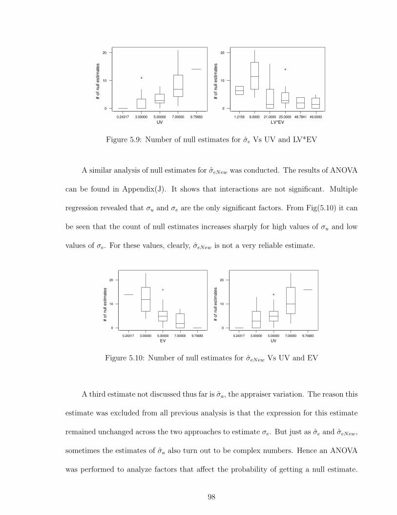
9.756837.000005.000003.000000.24317
20
10
0
UV
# o
f null e
stim
ate
s
49.000048.784125.000021.00009.00001.2159
20
10
0
LV*EV
# o
f null e
stim
ate
s
Figure 5.9: Number of null estimates for σe Vs UV and LV*EV
A similar analysis of null estimates for σeNew was conducted. The results of ANOVA
can be found in Appendix(J). It shows that interactions are not significant. Multiple
regression revealed that σu and σe are the only significant factors. From Fig(5.10) it can
be seen that the count of null estimates increases sharply for high values of σu and low
values of σe. For these values, clearly, σeNew is not a very reliable estimate.
9.756837.000005.000003.000000.24317
20
10
0
EV
# o
f null e
st im
ate
s
9.756837.000005.000003.000000.24317
20
10
0
UV
# o
f null e
stim
ate
s
Figure 5.10: Number of null estimates for σeNew Vs UV and EV
A third estimate not discussed thus far is σa, the appraiser variation. The reason this
estimate was excluded from all previous analysis is that the expression for this estimate
remained unchanged across the two approaches to estimate σe. But just as σe and σeNew,
sometimes the estimates of σa also turn out to be complex numbers. Hence an ANOVA
was performed to analyze factors that affect the probability of getting a null estimate.
98
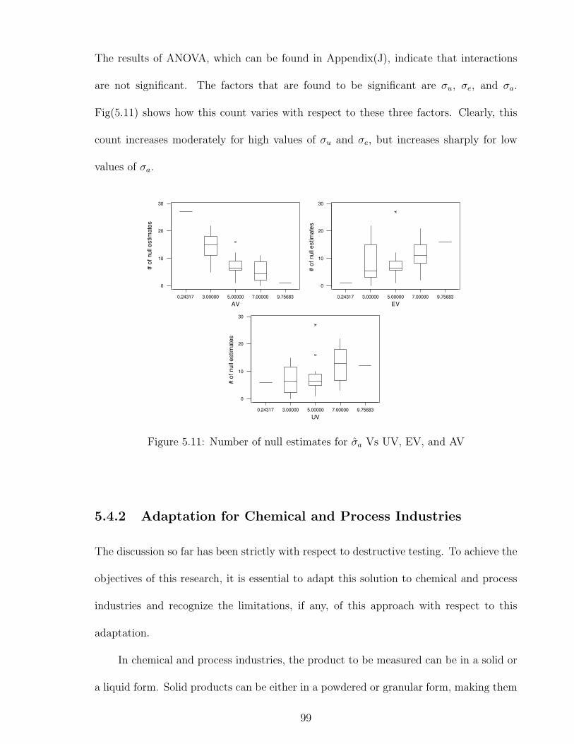
The results of ANOVA, which can be found in Appendix(J), indicate that interactions
are not significant. The factors that are found to be significant are σu, σe, and σa.
Fig(5.11) shows how this count varies with respect to these three factors. Clearly, this
count increases moderately for high values of σu and σe, but increases sharply for low
values of σa.
9.756837.000005.000003.000000.24317
30
20
10
0
AV
# o
f null e
st im
ate
s
9.756837.000005.000003.000000.24317
30
20
10
0
EV
# o
f null e
stim
ate
s
9.756837.000005.000003.000000.24317
30
20
10
0
UV
# o
f null e
st im
ate
s
Figure 5.11: Number of null estimates for σa Vs UV, EV, and AV
5.4.2 Adaptation for Chemical and Process Industries
The discussion so far has been strictly with respect to destructive testing. To achieve the
objectives of this research, it is essential to adapt this solution to chemical and process
industries and recognize the limitations, if any, of this approach with respect to this
adaptation.
In chemical and process industries, the product to be measured can be in a solid or
a liquid form. Solid products can be either in a powdered or granular form, making them
99
easy to be homogenized, or in the form of solid chunks (e.g., rubber), making them very
difficult to be homogenized.
First, consider product in the form of liquid or powdered/granular solid. The two
stage approach employed in this section, refers to units and locations within those units.
In Stage 1, 10 units are chosen randomly and 5 locations are chosen within each unit.
One appraiser measures all locations on all units. The locations are identical in each
unit to minimize the difference in the location effect of the same location on two different
units. In Stage 2, 3 appraisers measure 1 locations on 10 different units (a total of 30
units). In the context of chemical and process industries, the meaning of a unit can
vary from a truck load to a spoonfull depending on the context and the volume being
produced/handled. While it is not possible to address each specific industry separately,
a generic approach can be developed such that it can be used in various industries with
marginal modifications. The main steps in sample preparation are described below:
¦ Unit Selection. Define a unit as a barrel full of the product to be tested. A
total of 40 such barrels will be required—10 for Stage 1 and 30 for Stage 2. Choose
these barrels of the product randomly. If the product is not available in barrels,
fill ten barrels from the existing product, randomizing from barrel to barrel (not
within barrel) to the extent possible.
¦ Homogenization. Once such units are separated, each should be homogenized
to the extent possible. Homogenization should be attempted only after the units
(barrels) have been separated. This is essential in order to maintain detectable
unit-to-unit variation. Homogenizing a liquid product may be easier than doing
the same with a powdered or granular substance.
100
¦ Settling Period. After the previous step, the homogeneity of the unit will start
to change as a function of time. For example, if the characteristic of interest is
viscosity and the product is a liquid, then stirring the barrel will result in homog-
enization, but as soon as the stirring is stopped, the heavier particles will begin to
settle and cause the viscosity to have a gradient within the barrel. This gradient
will not be a problem by itself, as long as the time rate of change of viscosity is
small enough to be negligible with respect to the duration of the experiment (MSA
study). To attain this, the units should be left undisturbed for a certain period of
time. This time period should be chosen such that the rate of change of the char-
acteristic of interest is negligible with respect to the duration of the experiment.
In other words, it is necessary to ensure that location-to-location variation does
not change during the experiment. The time duration for which the units need to
be left undisturbed may vary from minutes to hours and the determination of this
time may pose the need for some additional experimentation. This problem may
be more serious in the case of liquid products.
¦ Location Definition. Locations should refer to actual physical locations in the
barrel. For Stage 1, use 3 locations per unit instead of five, thus selecting one
sample from the top, one from the center, and one from the bottom of the barrel.
These locations need to be precisely defined. A convenient way is to define them
in terms of coordinates with reference to the barrel geometry. For Stage 2, select
one sample form the top of the barrel.
¦ Sample Selection. The first sample should be selected from the center of the
top layer in the barrel. To obtain the second sample, the barrel should be emptied
101
until the the height of the product in the barrel is exactly half of the height of the
product before the first sample was taken. The second sample should be obtained
from the center of the surface of the product in the barrel. For the third sample a
similar process should be used. Care should be taken to allow sufficient material to
remain in the barrel for proper sample collection. Extreme care must be taken while
emptying the barrel to collect the second and the third sample in order to ensure
that no turbulence is introduced in the contents of the barrel. This is important to
maintain sample integrity.
¦ Sample Size. The size of the sample will be dictated by the product-type, char-
acteristic to be tested, and equipment to be used in testing. This sample size must
remain unchanged throughout the experiment. Care should be taken to ensure
that the size of the unit (barrel) is significantly larger (at least ten times) than the
sample size.
Some problems with the sample preparation approach described above, pertain to
accessibility and handling of the product, randomization, and maintaining sample in-
tegrity while emptying parts of the barrel to collect the second and the third sample for
Stage 1. The issue of accessibility arises if the product is not stored in barrels or similar
containers, but instead is stored in much larger containers such as rail-cars or is a liquid
that flows through pipelines. As suggested above, in such cases, barrels should be filled
for the purposes of the experiment. This raises the issue of randomization. Since such
large storages offer limited access points, true randomization is not possible. This may
cause the range of the true value of the characteristic to be measured to be very small
across the material collected for the experiment. Lack of unit-to-unit randomization will
102

not necessarily make the measurement error estimates unreliable. It will, however, limit
the validity of the results to the narrow range of the true value of the characteristic to be
measured. For example, if the true viscosity of the material collected for an experiment
ranges from 82cP to 84cP, whereas the expected range for the material being produced
is 78cP to 84cP. Based on the results of the experiment, there will be no way to estimate
how the measurement system will behave when encountered with a material of viscosity
78cP.
A significant challenge in adaptation of this process for chemical and process indus-
tries is posed by industries where the product is a solid that is difficult to homogenize
such as rubber. In such cases slabs of rubber can be taken and used as units. Chunks
of specific dimensions of rubber can be cut off from each slab from specific locations to
act as samples. A problem with this approach of sample preparation is that locations
on different units may not be as correlated as the two-stage approach assumes. In other
words, location 1 on unit 1 may not have the same location effect as location 1 on unit
2.
103
Chapter 6
Research Contributions and Summary
Chapter Overview
This chapter summarizes the key results and contributions of this research and draws
conclusions while reflecting on the objectives initially set.
6.1 Research Contributions
During the course of this research, it was realized that in the literature related to Mea-
surement System Analysis, there is a significant variation with respect to notation and
terminology. Some of these differences exist for a good reason—to distinguish among
subtle differences in the approach or the technique used. Inconsistent representation
however, has made it difficult to comprehend and compare these approaches. One of the
contributions of this dissertation is summarizing all schools of thought using consistent
notation and terminology.
There are two approaches for estimating variance components of measurement error—
range-based approach and ANOVA-based approach. Most authors recommend ANOVA-
based approach for superior accuracy. It has been established in this dissertation that
there is no statistically significant difference between the estimates obtained using either
approach. However, the range-based estimates may be sensitive assumptions such as
104
normality while ANOVA is robust to departures from normality. Increasing computing
power, wide use of computers in the industry, and support for MSA and/or ANOVA in
various statistics software have made using ANOVA both quicker and easier. It has also
been shown that EV is a more reliable estimate than AV.
This dissertation makes a strong case for the existence of within-appraiser variation
and its confounding with equipment variation. Lower bounds on average within-appraiser
variation and upper bounds on equipment variation have been estimated using two dif-
ferent approaches. Since these bounds are estimated based on expected values, they are
not fully effective. The effectiveness varies as the relative proportion of within-appraiser
variation and equipment variation in replication error changes. The bounds become more
effective as the former becomes the dominating component of replication error. Ignoring
within-appraiser variation can mean overestimating equipment variation, which in turn
may result in tampering with a potentially satisfactory measurement system. The ef-
fectiveness of these bounds has not been very satisfactory. This opens new avenues for
research in this area.
Traditionally, MSA studies have been done using a single measuring device or equip-
ment. In practice, however, it is possible that a given sample of parts is measured by
two appraisers on similar but different devices to save time. In such a case, observed
variation includes a component of measurement variation that the traditional analysis
will fail to catch—equipment-to-equipment variation. The appropriate linear model for
this scenario has been developed and guidelines have been given on whether equipment
should be treated as a random or a fixed factor in such an experiment. The estimates have
been tested for effectiveness. This approach has been developed using the ANOVA-based
approach.
105
The estimate of part-to-part variation given by AIAG was not accurate. This es-
timate has been corrected giving the theoretical background for such correction, and it
has been verified using simulation. The difference between the corrected estimate and
the traditional estimate, though statistically significant, is negligible from a practical
standpoint. This difference can increase for higher values of replication error, and lower
number replications and appraisers.
A number of criteria to assess measurement system acceptability have been suggested
in the literature. In this research, all these criteria have been simultaneously evaluated
under varying conditions of process capability and proportion of measurement variation in
the total or observed variation. The key findings are being summarized here. Using PTR
may produce results that are inconsistent with using DR or ndc. It should be realized
that even though both DR and PTR are criteria for measurement system acceptability,
they are measuring different quantities. Concerns over additivity of MV and PV in case
of criteria such as %TV and %MV have been addressed by using these ratios as ratios
of variances, and not standard deviations as is the general practice. Also, a DR of 5 as
recommended by AIAG corresponds to %TV = 7% when used as a ratio of variances and
27% when used as a ratio of standard deviations. The generally recommended threshold
for %TV is 10% which is closer to ratio based on variances. Great caution should be
exercised in using these criteria for evaluating a measurement system in practice. It
is easy to rule a good measurement system unacceptable due to nothing more than an
oversight.
Various approaches to dealing with a destructive measurement system have been
outlined in the literature. While most of these arrive at a solution by ignoring within-
sample variation, the approach developed by Mitchell et al. (1997) uses a two-stage
106
technique to arrive a solution. However, the way the data are collected in the second
stage is inconsistent with the linear model used for that stage. Moreover, the model in
Stage 1 is inconsistent with the model in Stage 2 with respect to certain key assumptions.
The models have been modified so that it is consistent not only with the model in Stage
1, but also with the way the data are collected. New estimates have been developed based
on these changes and their superiority with respect to the ones used by Mitchell et al.
(1997) has been demonstrated. Guidelines have been developed for using this technique,
originally developed with the semiconductor industry in mind, for MSA in chemical and
process industries.
6.2 Future Research
MSA research has matured significantly over the last few years, owing its growth primarily
to the pioneering efforts of AIAG in this field. However, there remain some opportuni-
ties for improvement to be discovered and some application areas to be explored. This
dissertation has addressed some such topics. In this section we will briefly touch upon
how some of these areas can be extended newer areas be explored.
Within-appraiser variation is an inevitable reality that has been ignored in all re-
search so far. It is nothing but the allowance for an operator or an appraiser to be
inconsistent in his/her operation—a concept that is in fact very intuitive and accept-
able. The lower bounds on the average within-appraiser variation are not very effective.
It would be ideal if it could be “unconfounded” from equipment variation, and accept-
able if more effective bounds could be developed so as to be used without running the
risk of overestimating it due to a bound-violation. An effective lower bound on within-
107
appraiser variation will automatically give us an effective upper bound on EV as they
are inextricably linked with each other.
Measurement system acceptability criteria evaluation in this dissertation has re-
vealed many interesting conflicts and redundancies. The point being made here is less
with respect to fundamental research in this area, and more about utilizing more re-
sources to educate the “quality-practitioners” with the pit-falls and risks of using these
without realizing their dependence on each other as well as on factors not directly related
to the measurement system, such as tolerance.
The adaptability of MSA for the chemical and process industries is an area where
there is significant potential for more research. These opportunities stem from the fact
that each industry and its product in this industry has some unique properties and
constraints that may need either minor customization of the approach used here, or a
complete overhaul of this process.
Some newer application areas for MSA need to be explored—education or similar
service industries for example. The author is not aware of any research, or lack thereof,
on MSA in these segments, but the idea of exploring the repeatability and reproducibility
of students and instructors does sound interesting!
108
Appendix A
Abbreviations
This appendix contains the expanded form of most abbreviations used in the text. The
abbreviations are alphabetically sorted and are accompanied by their symbolic represen-
tation wherever appropriate.
ANOVA Analysis of Variance
AV (σa) Appraiser Variation or Appraiser-to-Appraiser Variation
σa: Traditional estimate of AV
σaNew: Modified AV estimate provided by Montgomery and Runger
(1994a)
CCD Central Composite Design
CI Confidence Interval
cntE Number of null estimates of EV per 50 replications using the tradi-
tional approach of estimation for MSAD
cntENew Number of null estimates of EV per 50 replications using the new
approach (proposed as part of this research) of estimation for MSAD
109
cntA Number of null estimates of AV per 50 replications for
MSAD
DeltaE (∆e) Difference between true EV and the mean traditional es-
timate of EV (averaged over 50 replications in the text)
for MSAD
DeltaETrim
(∆eNew)
Difference between true EV and trimmed-mean of the tra-
ditional estimate of EV (averaged over 50 replications in
the text) for MSAD
DeltaENew
(∆eNew)
Difference between true EV and the mean of new estimate
of EV (averaged over 50 replications in the text) for MSAD
DeltaETrimNew
(∆eTrimNew)
Difference between true EV and trimmed-mean of new
estimate of EV (averaged over 50 replications in the text)
of MSAD
DR Discrimination Ratio
EMS Expected Mean Squares
ER Effective Resolution
EV (σe) Equipment Variation (typically within-equipment)
σe: Traditional estimate of EV
σeNew: Improved estimate of EV proposed in this research
for MSAD
LBa Lower Bound on average WIAV
110
LV (σl) Location-to-location variation (in MSAD)
MSAD Destructive Measurement System Analysis
MV (σm) Measurement Variation
ndc Number of Data/Distinct Categories
PE Probable Error
PTR Precision-to-Tolerance Ratio
PV (σp) Part Variation or Process Variation or Part-to-Part Variation
TC Treatment Combination
TV (σt) Total Variation (observed variation)
UBe Upper Bound on EV
UV (σu) Unit Variation or unit-to-unit variation (in MSAD)
VC Variance Component
WIAV (σaj) Within-Appraiser Variation
111
Appendix B
GUI Sample Screens
The software for simulating and testing the concepts presented in this dissertation was
developed in MATLAB. A Graphical User Interface was developed to allow the user
to manipulate the simulation parameters and view results and graphs in a convenient
manner. A master interface allows the user to choose the kind of application to run—
regular MSA, MSA with multiple devices, and MSA for destructive testing. This choice
opens up another interface for the specific application. A screen-shot of each of these
interfaces with a sample run is shown below.
112
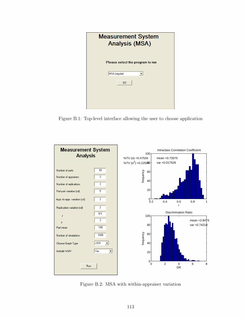
Figure B.1: Top-level interface allowing the user to choose application
0.2 0.4 0.6 0.8 10
20
40
60
80
100
r
freq
uenc
y
Intraclass Correlation Coefficient
%TV (σ) =0.47534
%TV (σ2) =0.22594
mean =0.73575
var =0.017526
0 2 4 6 80
20
40
60
80
100
DR
freq
uenc
y
Discrimination Ratio
mean =2.8474
var =0.74214
Figure B.2: MSA with within-appraiser variation
113
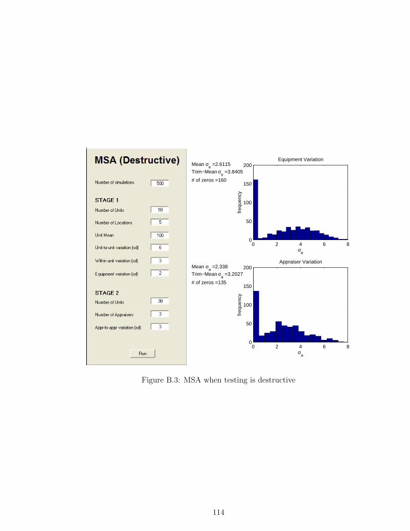
0 2 4 6 80
50
100
150
200
σe
freq
uenc
y
Equipment VariationMean σ
e =2.6115
Trim−Mean σe =3.8405
# of zeros =160
0 2 4 6 80
50
100
150
200
σa
freq
uenc
y
Appraiser VariationMean σ
a =2.338
Trim−Mean σa =3.2027
# of zeros =135
Figure B.3: MSA when testing is destructive
114
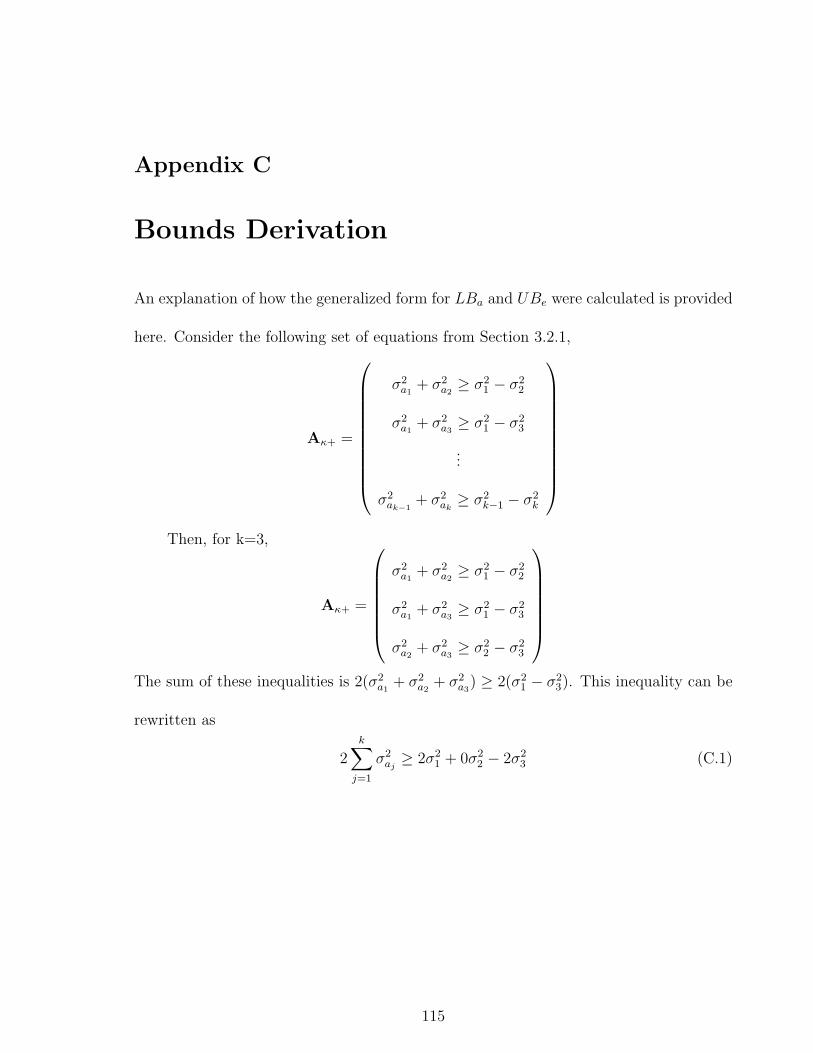
Appendix C
Bounds Derivation
An explanation of how the generalized form for LBa and UBe were calculated is provided
here. Consider the following set of equations from Section 3.2.1,
Aκ+ =
σ2a1
+ σ2a2≥ σ2
1 − σ22
σ2a1
+ σ2a3≥ σ2
1 − σ23
...
σ2ak−1
+ σ2ak≥ σ2
k−1 − σ2k
Then, for k=3,
Aκ+ =
σ2a1
+ σ2a2≥ σ2
1 − σ22
σ2a1
+ σ2a3≥ σ2
1 − σ23
σ2a2
+ σ2a3≥ σ2
2 − σ23
The sum of these inequalities is 2(σ2a1
+ σ2a2
+ σ2a3
) ≥ 2(σ21 − σ2
3). This inequality can be
rewritten as
2k∑
j=1
σ2aj≥ 2σ2
1 + 0σ22 − 2σ2
3 (C.1)
115
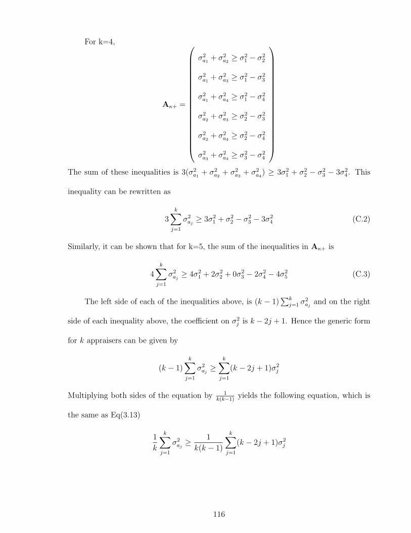
For k=4,
Aκ+ =
σ2a1
+ σ2a2≥ σ2
1 − σ22
σ2a1
+ σ2a3≥ σ2
1 − σ23
σ2a1
+ σ2a4≥ σ2
1 − σ24
σ2a2
+ σ2a3≥ σ2
2 − σ23
σ2a2
+ σ2a4≥ σ2
2 − σ24
σ2a3
+ σ2a4≥ σ2
3 − σ24
The sum of these inequalities is 3(σ2a1
+ σ2a2
+ σ2a3
+ σ2a4
) ≥ 3σ21 + σ2
2 − σ23 − 3σ2
4. This
inequality can be rewritten as
3k∑
j=1
σ2aj≥ 3σ2
1 + σ22 − σ2
3 − 3σ24 (C.2)
Similarly, it can be shown that for k=5, the sum of the inequalities in Aκ+ is
4k∑
j=1
σ2aj≥ 4σ2
1 + 2σ22 + 0σ2
3 − 2σ24 − 4σ2
5 (C.3)
The left side of each of the inequalities above, is (k − 1)∑k
j=1 σ2aj
and on the right
side of each inequality above, the coefficient on σ2j is k − 2j + 1. Hence the generic form
for k appraisers can be given by
(k − 1)k∑
j=1
σ2aj≥
k∑j=1
(k − 2j + 1)σ2j
Multiplying both sides of the equation by 1k(k−1)
yields the following equation, which is
the same as Eq(3.13)
1
k
k∑j=1
σ2aj≥ 1
k(k − 1)
k∑j=1
(k − 2j + 1)σ2j
116
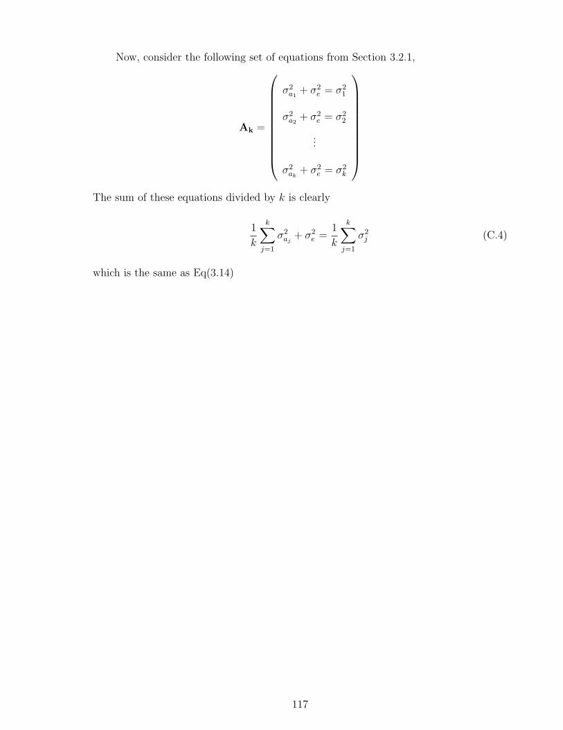
Now, consider the following set of equations from Section 3.2.1,
Ak =
σ2a1
+ σ2e = σ2
1
σ2a2
+ σ2e = σ2
2
...
σ2ak
+ σ2e = σ2
k
The sum of these equations divided by k is clearly
1
k
k∑j=1
σ2aj
+ σ2e =
1
k
k∑j=1
σ2j (C.4)
which is the same as Eq(3.14)
117
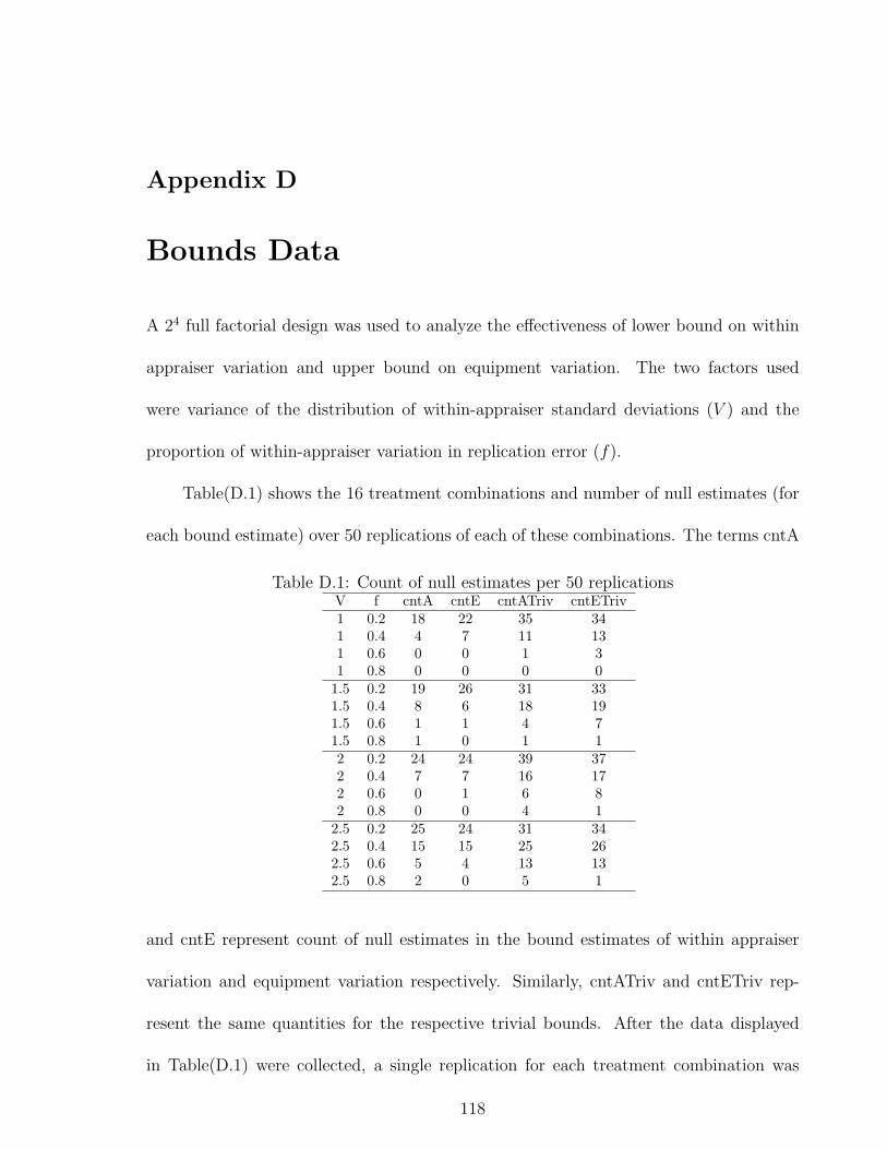
Appendix D
Bounds Data
A 24 full factorial design was used to analyze the effectiveness of lower bound on within
appraiser variation and upper bound on equipment variation. The two factors used
were variance of the distribution of within-appraiser standard deviations (V ) and the
proportion of within-appraiser variation in replication error (f).
Table(D.1) shows the 16 treatment combinations and number of null estimates (for
each bound estimate) over 50 replications of each of these combinations. The terms cntA
Table D.1: Count of null estimates per 50 replicationsV f cntA cntE cntATriv cntETriv1 0.2 18 22 35 341 0.4 4 7 11 131 0.6 0 0 1 31 0.8 0 0 0 0
1.5 0.2 19 26 31 331.5 0.4 8 6 18 191.5 0.6 1 1 4 71.5 0.8 1 0 1 12 0.2 24 24 39 372 0.4 7 7 16 172 0.6 0 1 6 82 0.8 0 0 4 1
2.5 0.2 25 24 31 342.5 0.4 15 15 25 262.5 0.6 5 4 13 132.5 0.8 2 0 5 1
and cntE represent count of null estimates in the bound estimates of within appraiser
variation and equipment variation respectively. Similarly, cntATriv and cntETriv rep-
resent the same quantities for the respective trivial bounds. After the data displayed
in Table(D.1) were collected, a single replication for each treatment combination was
118
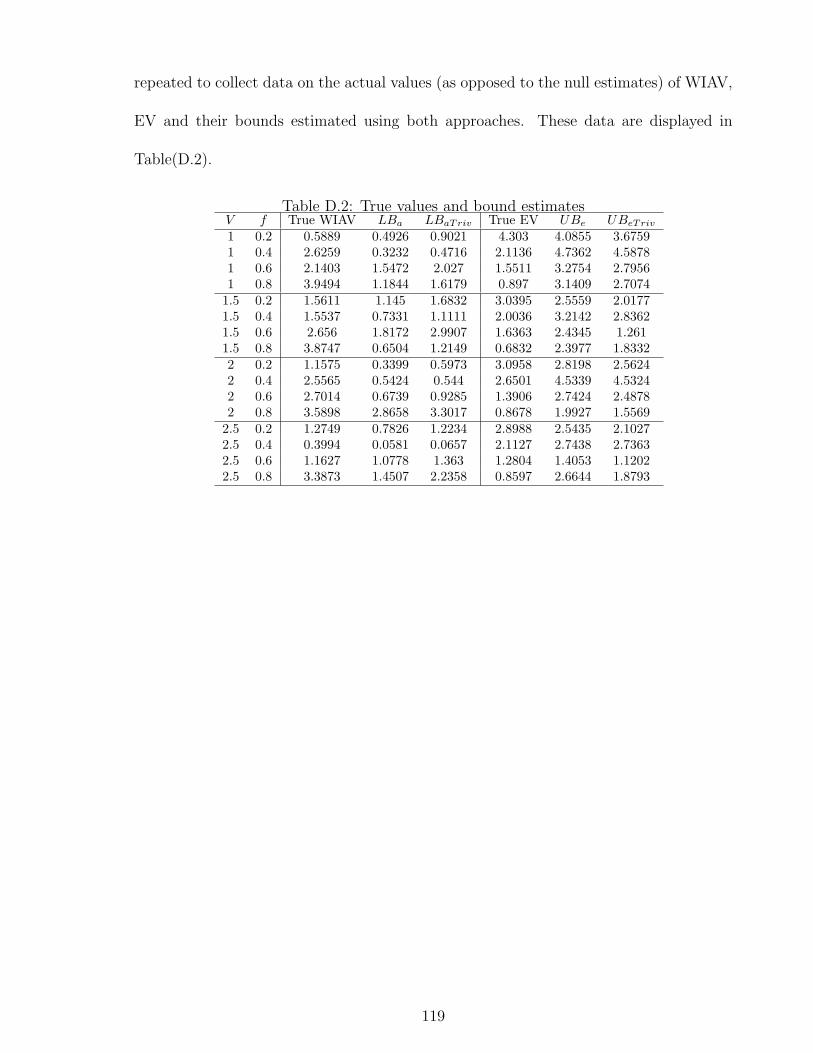
repeated to collect data on the actual values (as opposed to the null estimates) of WIAV,
EV and their bounds estimated using both approaches. These data are displayed in
Table(D.2).
Table D.2: True values and bound estimatesV f True WIAV LBa LBaTriv True EV UBe UBeTriv
1 0.2 0.5889 0.4926 0.9021 4.303 4.0855 3.67591 0.4 2.6259 0.3232 0.4716 2.1136 4.7362 4.58781 0.6 2.1403 1.5472 2.027 1.5511 3.2754 2.79561 0.8 3.9494 1.1844 1.6179 0.897 3.1409 2.7074
1.5 0.2 1.5611 1.145 1.6832 3.0395 2.5559 2.01771.5 0.4 1.5537 0.7331 1.1111 2.0036 3.2142 2.83621.5 0.6 2.656 1.8172 2.9907 1.6363 2.4345 1.2611.5 0.8 3.8747 0.6504 1.2149 0.6832 2.3977 1.83322 0.2 1.1575 0.3399 0.5973 3.0958 2.8198 2.56242 0.4 2.5565 0.5424 0.544 2.6501 4.5339 4.53242 0.6 2.7014 0.6739 0.9285 1.3906 2.7424 2.48782 0.8 3.5898 2.8658 3.3017 0.8678 1.9927 1.5569
2.5 0.2 1.2749 0.7826 1.2234 2.8988 2.5435 2.10272.5 0.4 0.3994 0.0581 0.0657 2.1127 2.7438 2.73632.5 0.6 1.1627 1.0778 1.363 1.2804 1.4053 1.12022.5 0.8 3.3873 1.4507 2.2358 0.8597 2.6644 1.8793
119
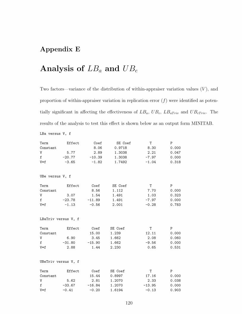
Appendix E
Analysis of LBa and UBe
Two factors—variance of the distribution of within-appraiser variation values (V ), and
proportion of within-appraiser variation in replication error (f) were identified as poten-
tially significant in affecting the effectiveness of LBa, UBe, LBaTriv and UBeTriv. The
results of the analysis to test this effect is shown below as an output form MINITAB.
LBa versus V, f
Term Effect Coef SE Coef T PConstant 8.06 0.9718 8.30 0.000V 5.77 2.89 1.3038 2.21 0.047f -20.77 -10.39 1.3038 -7.97 0.000V*f -3.65 -1.82 1.7492 -1.04 0.318
UBe versus V, f
Term Effect Coef SE Coef T PConstant 8.56 1.112 7.70 0.000V 3.07 1.54 1.491 1.03 0.323f -23.78 -11.89 1.491 -7.97 0.000V*f -1.13 -0.56 2.001 -0.28 0.783
LBaTriv versus V, f
Term Effect Coef SE Coef T PConstant 15.00 1.239 12.11 0.000V 6.90 3.45 1.662 2.08 0.060f -31.80 -15.90 1.662 -9.56 0.000V*f 2.88 1.44 2.230 0.65 0.531
UBeTriv versus V, f
Term Effect Coef SE Coef T PConstant 15.44 0.8997 17.16 0.000V 5.62 2.81 1.2070 2.33 0.038f -33.67 -16.84 1.2070 -13.95 0.000V*f -0.41 -0.20 1.6194 -0.13 0.903
120
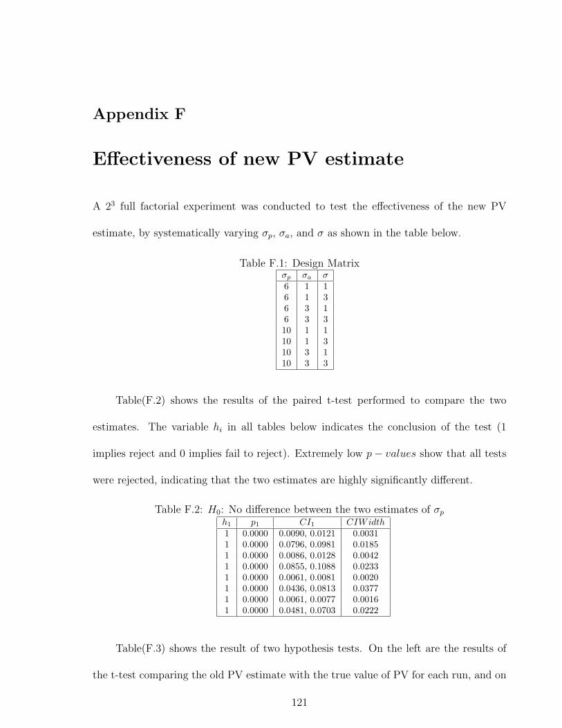
Appendix F
Effectiveness of new PV estimate
A 23 full factorial experiment was conducted to test the effectiveness of the new PV
estimate, by systematically varying σp, σa, and σ as shown in the table below.
Table F.1: Design Matrixσp σa σ6 1 16 1 36 3 16 3 310 1 110 1 310 3 110 3 3
Table(F.2) shows the results of the paired t-test performed to compare the two
estimates. The variable hi in all tables below indicates the conclusion of the test (1
implies reject and 0 implies fail to reject). Extremely low p− values show that all tests
were rejected, indicating that the two estimates are highly significantly different.
Table F.2: H0: No difference between the two estimates of σp
h1 p1 CI1 CIWidth1 0.0000 0.0090, 0.0121 0.00311 0.0000 0.0796, 0.0981 0.01851 0.0000 0.0086, 0.0128 0.00421 0.0000 0.0855, 0.1088 0.02331 0.0000 0.0061, 0.0081 0.00201 0.0000 0.0436, 0.0813 0.03771 0.0000 0.0061, 0.0077 0.00161 0.0000 0.0481, 0.0703 0.0222
Table(F.3) shows the result of two hypothesis tests. On the left are the results of
the t-test comparing the old PV estimate with the true value of PV for each run, and on
121
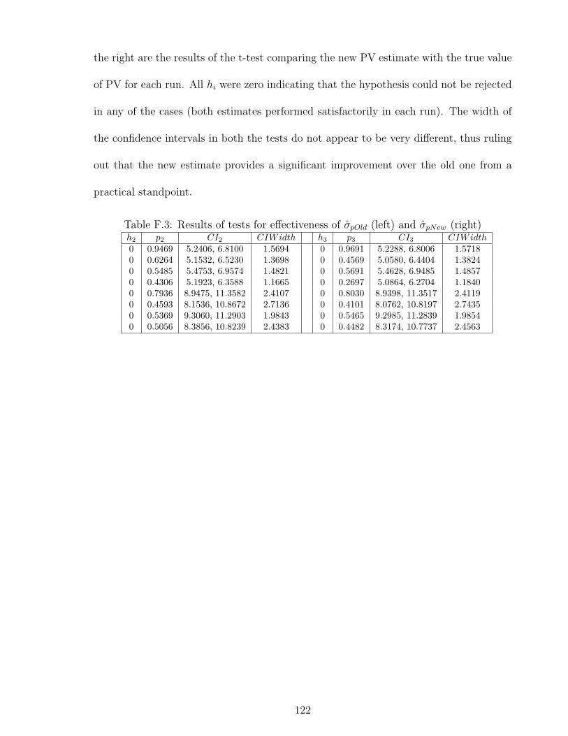
the right are the results of the t-test comparing the new PV estimate with the true value
of PV for each run. All hi were zero indicating that the hypothesis could not be rejected
in any of the cases (both estimates performed satisfactorily in each run). The width of
the confidence intervals in both the tests do not appear to be very different, thus ruling
out that the new estimate provides a significant improvement over the old one from a
practical standpoint.
Table F.3: Results of tests for effectiveness of σpOld (left) and σpNew (right)h2 p2 CI2 CIWidth h3 p3 CI3 CIWidth0 0.9469 5.2406, 6.8100 1.5694 0 0.9691 5.2288, 6.8006 1.57180 0.6264 5.1532, 6.5230 1.3698 0 0.4569 5.0580, 6.4404 1.38240 0.5485 5.4753, 6.9574 1.4821 0 0.5691 5.4628, 6.9485 1.48570 0.4306 5.1923, 6.3588 1.1665 0 0.2697 5.0864, 6.2704 1.18400 0.7936 8.9475, 11.3582 2.4107 0 0.8030 8.9398, 11.3517 2.41190 0.4593 8.1536, 10.8672 2.7136 0 0.4101 8.0762, 10.8197 2.74350 0.5369 9.3060, 11.2903 1.9843 0 0.5465 9.2985, 11.2839 1.98540 0.5056 8.3856, 10.8239 2.4383 0 0.4482 8.3174, 10.7737 2.4563
122
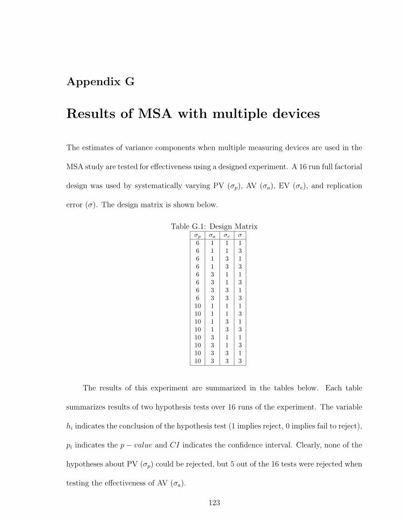
Appendix G
Results of MSA with multiple devices
The estimates of variance components when multiple measuring devices are used in the
MSA study are tested for effectiveness using a designed experiment. A 16 run full factorial
design was used by systematically varying PV (σp), AV (σa), EV (σe), and replication
error (σ). The design matrix is shown below.
Table G.1: Design Matrixσp σa σe σ6 1 1 16 1 1 36 1 3 16 1 3 36 3 1 16 3 1 36 3 3 16 3 3 310 1 1 110 1 1 310 1 3 110 1 3 310 3 1 110 3 1 310 3 3 110 3 3 3
The results of this experiment are summarized in the tables below. Each table
summarizes results of two hypothesis tests over 16 runs of the experiment. The variable
hi indicates the conclusion of the hypothesis test (1 implies reject, 0 implies fail to reject),
pi indicates the p− value and CI indicates the confidence interval. Clearly, none of the
hypotheses about PV (σp) could be rejected, but 5 out of the 16 tests were rejected when
testing the effectiveness of AV (σa).
123
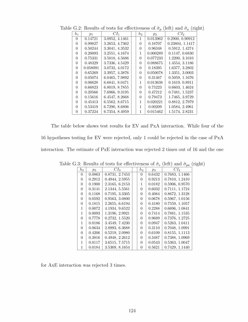
Table G.2: Results of tests for effectiveness of σp (left) and σa (right)h1 p1 CI1 h2 p2 CI2
0 0.14721 3.0952, 4.1461 1 0.013962 0.2900, 0.909120 0.99827 3.2653, 4.7362 0 0.16707 0.23804, 1.14170 0.50244 3.3041, 4.3532 0 0.96348 0.5912, 1.42740 0.20093 3.2551, 4.1674 1 0.000289 0.1147, 0.68300 0.75331 3.5818, 4.5686 0 0.077233 1.2200, 3.10100 0.48329 3.7336, 4.5429 0 0.088675 1.4554, 3.11860 0.058091 3.0732, 4.0172 0 0.18395 1.6377, 3.28020 0.65269 3.3957, 4.3876 0 0.050078 1.3351, 3.00030 0.05074 6.0465, 7.9892 0 0.31467 0.5059, 1.16760 0.06628 6.6841, 8.0471 1 0.013638 0.1619, 0.89110 0.66823 6.8019, 8.7855 0 0.75223 0.6603, 1.46240 0.20566 7.6966, 9.3195 0 0.47212 0.7481, 1.52370 0.15616 6.4547, 8.2668 0 0.79473 1.7465, 3.97290 0.45413 6.5562, 8.6715 1 0.020221 0.8812, 2.79790 0.53419 6.7290, 8.6806 1 0.00209 1.0584, 2.49610 0.37224 6.7354, 8.4959 1 0.015462 1.5174, 2.8231
The table below shows test results for EV and PxA interaction. While four of the
16 hypotheses testing for EV were rejected, only 1 could be rejected in the case of PxA
interaction. The estimate of PxE interaction was rejected 2 times out of 16 and the one
Table G.3: Results of tests for effectiveness of σe (left) and σpa (right)h3 p3 CI3 h4 p4 CI4
0 0.0863 0.8731, 2.7453 0 0.6432 0.7683, 1.14660 0.2912 0.4944, 2.5955 0 0.9213 0.7810, 1.24100 0.1900 2.3165, 6.2153 1 0.0182 0.5906, 0.95700 0.3141 2.1344, 5.5561 0 0.6032 0.7111, 1.17240 0.1168 0.7195, 3.3305 0 0.4084 0.8672, 1.31280 0.0592 0.9563, 3.0800 0 0.0678 0.5967, 1.01560 0.1815 2.2655, 6.6194 0 0.4180 0.7559, 1.10571 0.0072 4.1934, 9.6522 0 0.2288 0.6696, 1.08411 0.0093 1.3196, 2.9921 0 0.7414 0.7881, 1.15350 0.7778 0.2732, 1.5520 0 0.9689 0.7376, 1.27251 0.0186 3.4549, 7.4230 0 0.0947 0.5263, 1.04110 0.0634 2.8993, 6.3688 0 0.3110 0.7048, 1.09910 0.4206 0.5219, 2.0980 0 0.6109 0.8155, 1.11130 0.3816 0.4948, 2.2612 0 0.3487 0.7388, 1.09691 0.0117 3.6515, 7.5715 0 0.0543 0.5363, 1.00471 0.0184 3.5369, 8.1654 0 0.5621 0.7429, 1.1440
for AxE interaction was rejected 3 times.
124
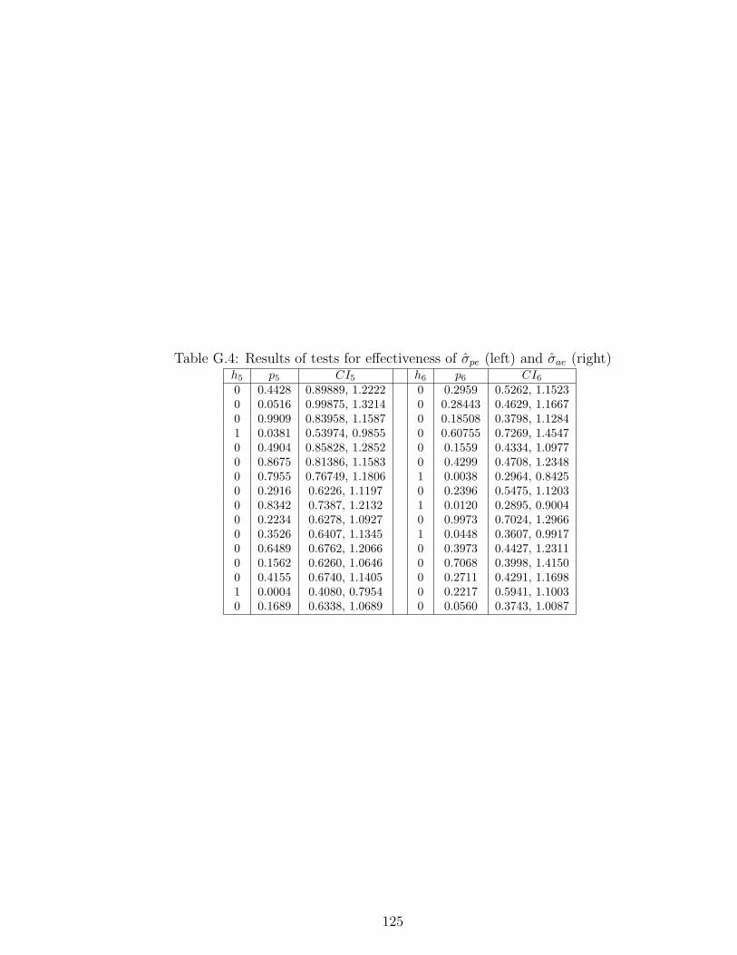
Table G.4: Results of tests for effectiveness of σpe (left) and σae (right)h5 p5 CI5 h6 p6 CI6
0 0.4428 0.89889, 1.2222 0 0.2959 0.5262, 1.15230 0.0516 0.99875, 1.3214 0 0.28443 0.4629, 1.16670 0.9909 0.83958, 1.1587 0 0.18508 0.3798, 1.12841 0.0381 0.53974, 0.9855 0 0.60755 0.7269, 1.45470 0.4904 0.85828, 1.2852 0 0.1559 0.4334, 1.09770 0.8675 0.81386, 1.1583 0 0.4299 0.4708, 1.23480 0.7955 0.76749, 1.1806 1 0.0038 0.2964, 0.84250 0.2916 0.6226, 1.1197 0 0.2396 0.5475, 1.12030 0.8342 0.7387, 1.2132 1 0.0120 0.2895, 0.90040 0.2234 0.6278, 1.0927 0 0.9973 0.7024, 1.29660 0.3526 0.6407, 1.1345 1 0.0448 0.3607, 0.99170 0.6489 0.6762, 1.2066 0 0.3973 0.4427, 1.23110 0.1562 0.6260, 1.0646 0 0.7068 0.3998, 1.41500 0.4155 0.6740, 1.1405 0 0.2711 0.4291, 1.16981 0.0004 0.4080, 0.7954 0 0.2217 0.5941, 1.10030 0.1689 0.6338, 1.0689 0 0.0560 0.3743, 1.0087
125
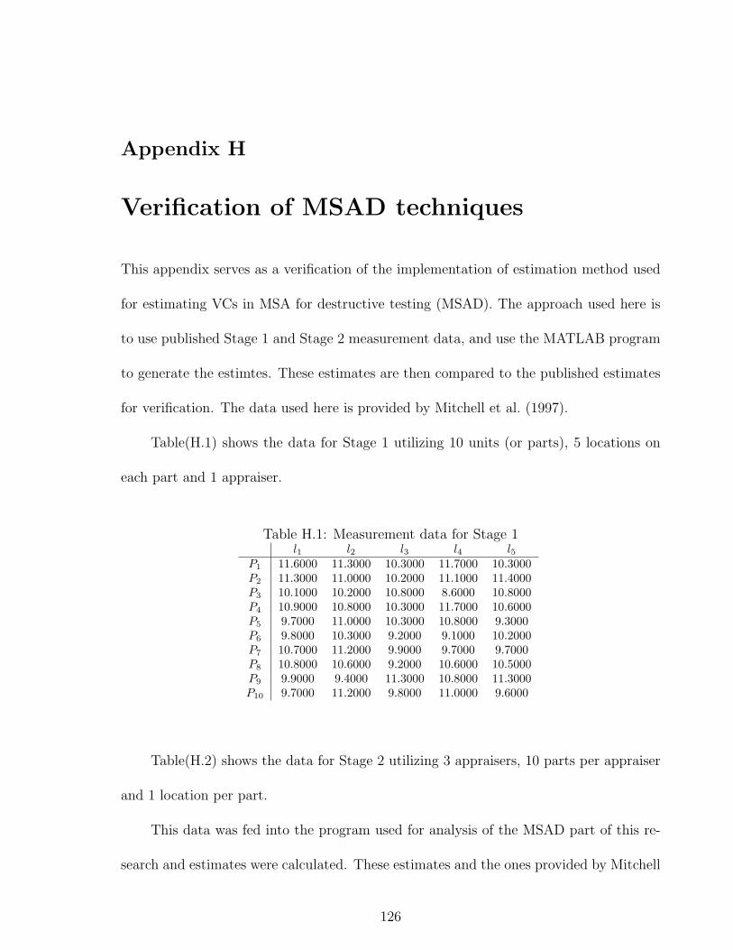
Appendix H
Verification of MSAD techniques
This appendix serves as a verification of the implementation of estimation method used
for estimating VCs in MSA for destructive testing (MSAD). The approach used here is
to use published Stage 1 and Stage 2 measurement data, and use the MATLAB program
to generate the estimtes. These estimates are then compared to the published estimates
for verification. The data used here is provided by Mitchell et al. (1997).
Table(H.1) shows the data for Stage 1 utilizing 10 units (or parts), 5 locations on
each part and 1 appraiser.
Table H.1: Measurement data for Stage 1l1 l2 l3 l4 l5
P1 11.6000 11.3000 10.3000 11.7000 10.3000P2 11.3000 11.0000 10.2000 11.1000 11.4000P3 10.1000 10.2000 10.8000 8.6000 10.8000P4 10.9000 10.8000 10.3000 11.7000 10.6000P5 9.7000 11.0000 10.3000 10.8000 9.3000P6 9.8000 10.3000 9.2000 9.1000 10.2000P7 10.7000 11.2000 9.9000 9.7000 9.7000P8 10.8000 10.6000 9.2000 10.6000 10.5000P9 9.9000 9.4000 11.3000 10.8000 11.3000P10 9.7000 11.2000 9.8000 11.0000 9.6000
Table(H.2) shows the data for Stage 2 utilizing 3 appraisers, 10 parts per appraiser
and 1 location per part.
This data was fed into the program used for analysis of the MSAD part of this re-
search and estimates were calculated. These estimates and the ones provided by Mitchell
126
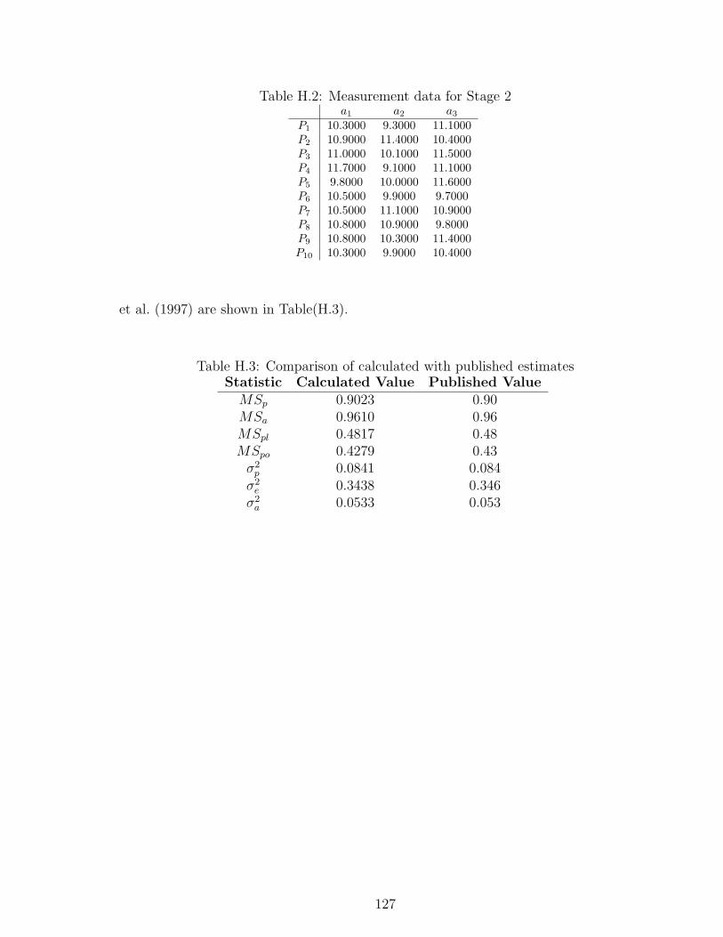
Table H.2: Measurement data for Stage 2a1 a2 a3
P1 10.3000 9.3000 11.1000P2 10.9000 11.4000 10.4000P3 11.0000 10.1000 11.5000P4 11.7000 9.1000 11.1000P5 9.8000 10.0000 11.6000P6 10.5000 9.9000 9.7000P7 10.5000 11.1000 10.9000P8 10.8000 10.9000 9.8000P9 10.8000 10.3000 11.4000P10 10.3000 9.9000 10.4000
et al. (1997) are shown in Table(H.3).
Table H.3: Comparison of calculated with published estimatesStatistic Calculated Value Published Value
MSp 0.9023 0.90MSa 0.9610 0.96MSpl 0.4817 0.48MSpo 0.4279 0.43
σ2p 0.0841 0.084
σ2e 0.3438 0.346
σ2a 0.0533 0.053
127
Appendix I
MSAD Output
A 4 factor 52 run CCD was performed to test various hypotheses regarding the destructive
MSA techniques. The design matrix is shown in Table(I.1). The subsequent tables
illustrate the summary statistics of this experiment outlining the results of hypothesis
tests conducted for each TC. In these tables hi indicates whether the hypothesis was
rejected or not (1 implies reject and 0 implies fail to reject). Similarly pi and CIi represent
the p-value associated with the hypothesis test and the appropriate confidence interval,
respectively.
Table(I.2) shows the results of the hypothesis testing whether the two approaches of
calculating EV are significantly different from each other. Table(I.3) shows test results
comparing the two EV estimates to the true value for each run. Some estimates of EV2
turned out to be negative due to the method of estimation. In such cases the estimate
of EV was considered to be zero. Table(I.4) tests the same hypothesis as Table(I.3) but
with trimmed mean instead of the overall mean. Trimmed mean of the estimate is the
mean after removing zeros from the analysis.
128
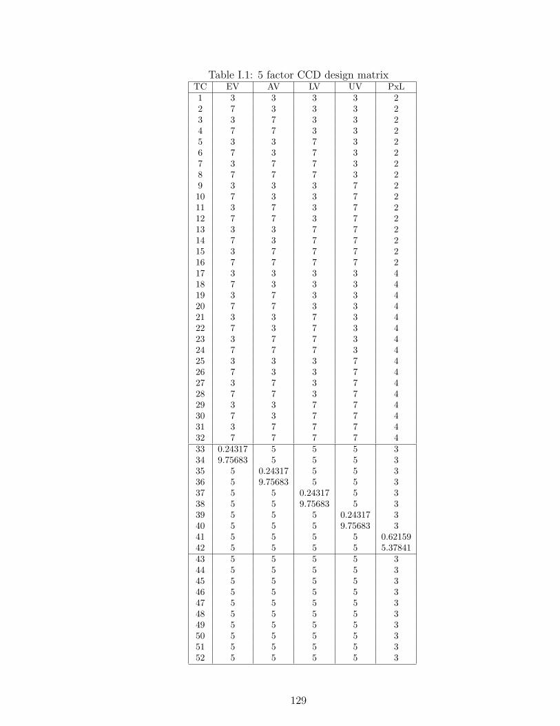
Table I.1: 5 factor CCD design matrixTC EV AV LV UV PxL1 3 3 3 3 22 7 3 3 3 23 3 7 3 3 24 7 7 3 3 25 3 3 7 3 26 7 3 7 3 27 3 7 7 3 28 7 7 7 3 29 3 3 3 7 210 7 3 3 7 211 3 7 3 7 212 7 7 3 7 213 3 3 7 7 214 7 3 7 7 215 3 7 7 7 216 7 7 7 7 217 3 3 3 3 418 7 3 3 3 419 3 7 3 3 420 7 7 3 3 421 3 3 7 3 422 7 3 7 3 423 3 7 7 3 424 7 7 7 3 425 3 3 3 7 426 7 3 3 7 427 3 7 3 7 428 7 7 3 7 429 3 3 7 7 430 7 3 7 7 431 3 7 7 7 432 7 7 7 7 433 0.24317 5 5 5 334 9.75683 5 5 5 335 5 0.24317 5 5 336 5 9.75683 5 5 337 5 5 0.24317 5 338 5 5 9.75683 5 339 5 5 5 0.24317 340 5 5 5 9.75683 341 5 5 5 5 0.6215942 5 5 5 5 5.3784143 5 5 5 5 344 5 5 5 5 345 5 5 5 5 346 5 5 5 5 347 5 5 5 5 348 5 5 5 5 349 5 5 5 5 350 5 5 5 5 351 5 5 5 5 352 5 5 5 5 3
129
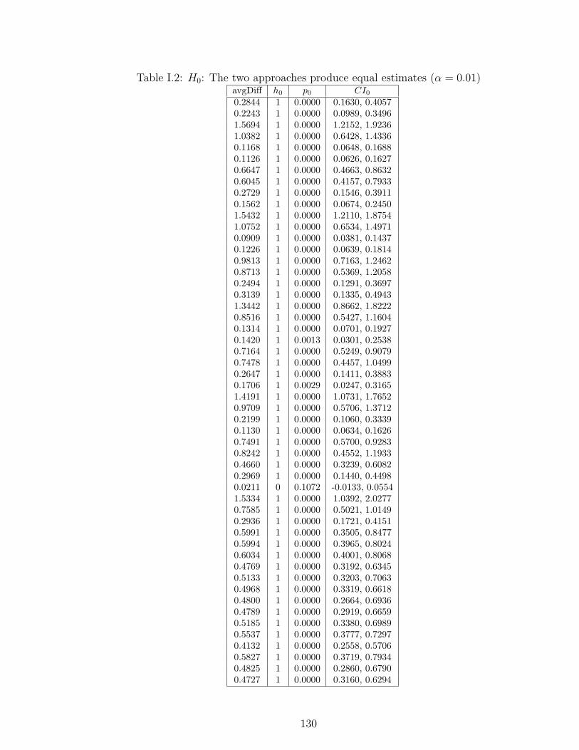
Table I.2: H0: The two approaches produce equal estimates (α = 0.01)avgDiff h0 p0 CI0
0.2844 1 0.0000 0.1630, 0.40570.2243 1 0.0000 0.0989, 0.34961.5694 1 0.0000 1.2152, 1.92361.0382 1 0.0000 0.6428, 1.43360.1168 1 0.0000 0.0648, 0.16880.1126 1 0.0000 0.0626, 0.16270.6647 1 0.0000 0.4663, 0.86320.6045 1 0.0000 0.4157, 0.79330.2729 1 0.0000 0.1546, 0.39110.1562 1 0.0000 0.0674, 0.24501.5432 1 0.0000 1.2110, 1.87541.0752 1 0.0000 0.6534, 1.49710.0909 1 0.0000 0.0381, 0.14370.1226 1 0.0000 0.0639, 0.18140.9813 1 0.0000 0.7163, 1.24620.8713 1 0.0000 0.5369, 1.20580.2494 1 0.0000 0.1291, 0.36970.3139 1 0.0000 0.1335, 0.49431.3442 1 0.0000 0.8662, 1.82220.8516 1 0.0000 0.5427, 1.16040.1314 1 0.0000 0.0701, 0.19270.1420 1 0.0013 0.0301, 0.25380.7164 1 0.0000 0.5249, 0.90790.7478 1 0.0000 0.4457, 1.04990.2647 1 0.0000 0.1411, 0.38830.1706 1 0.0029 0.0247, 0.31651.4191 1 0.0000 1.0731, 1.76520.9709 1 0.0000 0.5706, 1.37120.2199 1 0.0000 0.1060, 0.33390.1130 1 0.0000 0.0634, 0.16260.7491 1 0.0000 0.5700, 0.92830.8242 1 0.0000 0.4552, 1.19330.4660 1 0.0000 0.3239, 0.60820.2969 1 0.0000 0.1440, 0.44980.0211 0 0.1072 -0.0133, 0.05541.5334 1 0.0000 1.0392, 2.02770.7585 1 0.0000 0.5021, 1.01490.2936 1 0.0000 0.1721, 0.41510.5991 1 0.0000 0.3505, 0.84770.5994 1 0.0000 0.3965, 0.80240.6034 1 0.0000 0.4001, 0.80680.4769 1 0.0000 0.3192, 0.63450.5133 1 0.0000 0.3203, 0.70630.4968 1 0.0000 0.3319, 0.66180.4800 1 0.0000 0.2664, 0.69360.4789 1 0.0000 0.2919, 0.66590.5185 1 0.0000 0.3380, 0.69890.5537 1 0.0000 0.3777, 0.72970.4132 1 0.0000 0.2558, 0.57060.5827 1 0.0000 0.3719, 0.79340.4825 1 0.0000 0.2860, 0.67900.4727 1 0.0000 0.3160, 0.6294
130
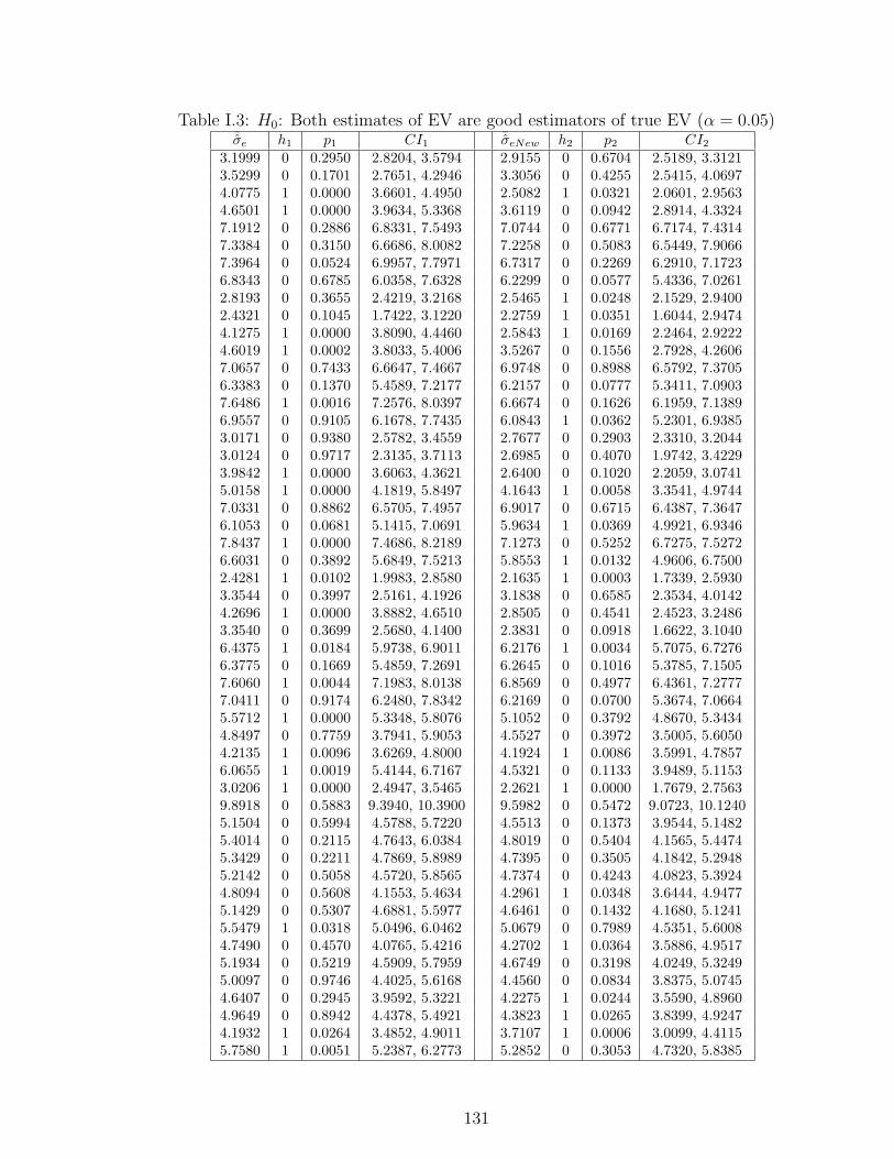
Table I.3: H0: Both estimates of EV are good estimators of true EV (α = 0.05)¯σe h1 p1 CI1
¯σeNew h2 p2 CI2
3.1999 0 0.2950 2.8204, 3.5794 2.9155 0 0.6704 2.5189, 3.31213.5299 0 0.1701 2.7651, 4.2946 3.3056 0 0.4255 2.5415, 4.06974.0775 1 0.0000 3.6601, 4.4950 2.5082 1 0.0321 2.0601, 2.95634.6501 1 0.0000 3.9634, 5.3368 3.6119 0 0.0942 2.8914, 4.33247.1912 0 0.2886 6.8331, 7.5493 7.0744 0 0.6771 6.7174, 7.43147.3384 0 0.3150 6.6686, 8.0082 7.2258 0 0.5083 6.5449, 7.90667.3964 0 0.0524 6.9957, 7.7971 6.7317 0 0.2269 6.2910, 7.17236.8343 0 0.6785 6.0358, 7.6328 6.2299 0 0.0577 5.4336, 7.02612.8193 0 0.3655 2.4219, 3.2168 2.5465 1 0.0248 2.1529, 2.94002.4321 0 0.1045 1.7422, 3.1220 2.2759 1 0.0351 1.6044, 2.94744.1275 1 0.0000 3.8090, 4.4460 2.5843 1 0.0169 2.2464, 2.92224.6019 1 0.0002 3.8033, 5.4006 3.5267 0 0.1556 2.7928, 4.26067.0657 0 0.7433 6.6647, 7.4667 6.9748 0 0.8988 6.5792, 7.37056.3383 0 0.1370 5.4589, 7.2177 6.2157 0 0.0777 5.3411, 7.09037.6486 1 0.0016 7.2576, 8.0397 6.6674 0 0.1626 6.1959, 7.13896.9557 0 0.9105 6.1678, 7.7435 6.0843 1 0.0362 5.2301, 6.93853.0171 0 0.9380 2.5782, 3.4559 2.7677 0 0.2903 2.3310, 3.20443.0124 0 0.9717 2.3135, 3.7113 2.6985 0 0.4070 1.9742, 3.42293.9842 1 0.0000 3.6063, 4.3621 2.6400 0 0.1020 2.2059, 3.07415.0158 1 0.0000 4.1819, 5.8497 4.1643 1 0.0058 3.3541, 4.97447.0331 0 0.8862 6.5705, 7.4957 6.9017 0 0.6715 6.4387, 7.36476.1053 0 0.0681 5.1415, 7.0691 5.9634 1 0.0369 4.9921, 6.93467.8437 1 0.0000 7.4686, 8.2189 7.1273 0 0.5252 6.7275, 7.52726.6031 0 0.3892 5.6849, 7.5213 5.8553 1 0.0132 4.9606, 6.75002.4281 1 0.0102 1.9983, 2.8580 2.1635 1 0.0003 1.7339, 2.59303.3544 0 0.3997 2.5161, 4.1926 3.1838 0 0.6585 2.3534, 4.01424.2696 1 0.0000 3.8882, 4.6510 2.8505 0 0.4541 2.4523, 3.24863.3540 0 0.3699 2.5680, 4.1400 2.3831 0 0.0918 1.6622, 3.10406.4375 1 0.0184 5.9738, 6.9011 6.2176 1 0.0034 5.7075, 6.72766.3775 0 0.1669 5.4859, 7.2691 6.2645 0 0.1016 5.3785, 7.15057.6060 1 0.0044 7.1983, 8.0138 6.8569 0 0.4977 6.4361, 7.27777.0411 0 0.9174 6.2480, 7.8342 6.2169 0 0.0700 5.3674, 7.06645.5712 1 0.0000 5.3348, 5.8076 5.1052 0 0.3792 4.8670, 5.34344.8497 0 0.7759 3.7941, 5.9053 4.5527 0 0.3972 3.5005, 5.60504.2135 1 0.0096 3.6269, 4.8000 4.1924 1 0.0086 3.5991, 4.78576.0655 1 0.0019 5.4144, 6.7167 4.5321 0 0.1133 3.9489, 5.11533.0206 1 0.0000 2.4947, 3.5465 2.2621 1 0.0000 1.7679, 2.75639.8918 0 0.5883 9.3940, 10.3900 9.5982 0 0.5472 9.0723, 10.12405.1504 0 0.5994 4.5788, 5.7220 4.5513 0 0.1373 3.9544, 5.14825.4014 0 0.2115 4.7643, 6.0384 4.8019 0 0.5404 4.1565, 5.44745.3429 0 0.2211 4.7869, 5.8989 4.7395 0 0.3505 4.1842, 5.29485.2142 0 0.5058 4.5720, 5.8565 4.7374 0 0.4243 4.0823, 5.39244.8094 0 0.5608 4.1553, 5.4634 4.2961 1 0.0348 3.6444, 4.94775.1429 0 0.5307 4.6881, 5.5977 4.6461 0 0.1432 4.1680, 5.12415.5479 1 0.0318 5.0496, 6.0462 5.0679 0 0.7989 4.5351, 5.60084.7490 0 0.4570 4.0765, 5.4216 4.2702 1 0.0364 3.5886, 4.95175.1934 0 0.5219 4.5909, 5.7959 4.6749 0 0.3198 4.0249, 5.32495.0097 0 0.9746 4.4025, 5.6168 4.4560 0 0.0834 3.8375, 5.07454.6407 0 0.2945 3.9592, 5.3221 4.2275 1 0.0244 3.5590, 4.89604.9649 0 0.8942 4.4378, 5.4921 4.3823 1 0.0265 3.8399, 4.92474.1932 1 0.0264 3.4852, 4.9011 3.7107 1 0.0006 3.0099, 4.41155.7580 1 0.0051 5.2387, 6.2773 5.2852 0 0.3053 4.7320, 5.8385
131
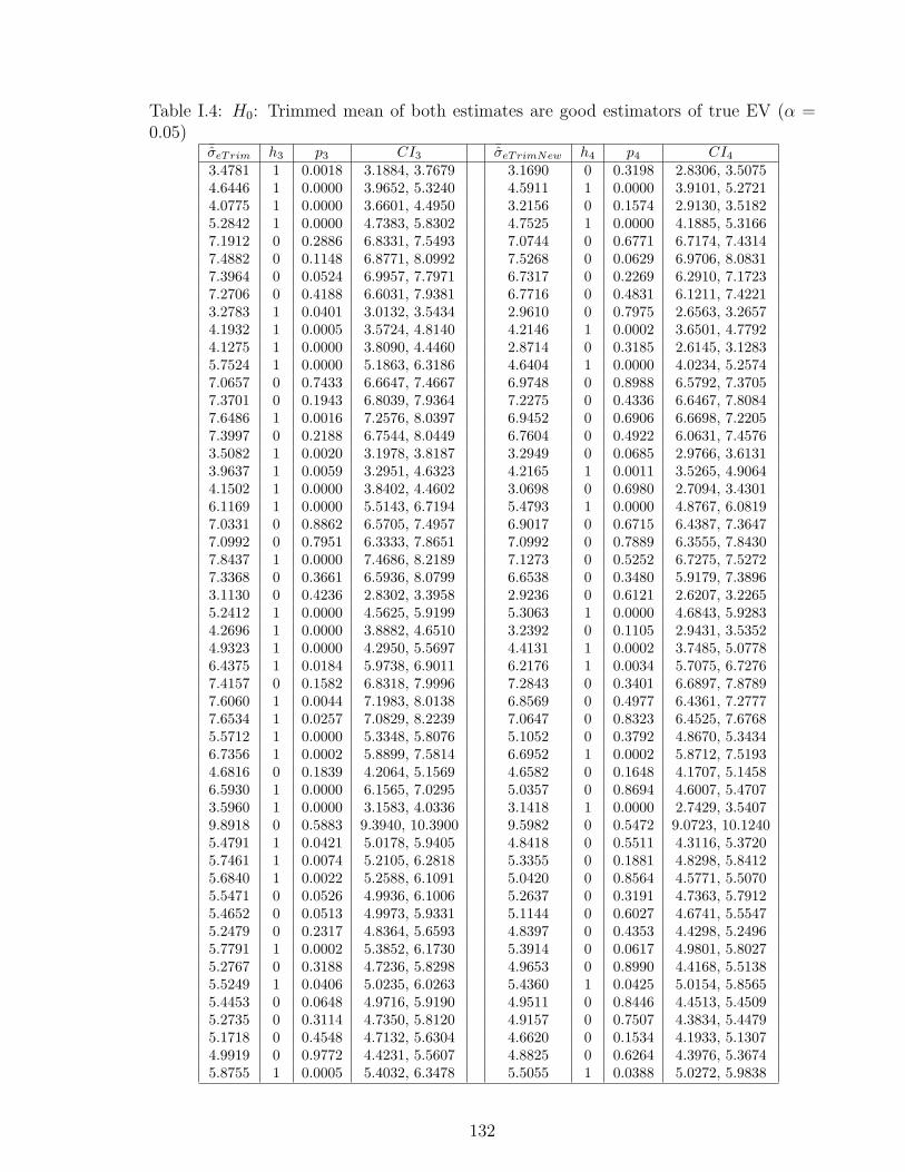
Table I.4: H0: Trimmed mean of both estimates are good estimators of true EV (α =0.05)
¯σeTrim h3 p3 CI3¯σeTrimNew h4 p4 CI4
3.4781 1 0.0018 3.1884, 3.7679 3.1690 0 0.3198 2.8306, 3.50754.6446 1 0.0000 3.9652, 5.3240 4.5911 1 0.0000 3.9101, 5.27214.0775 1 0.0000 3.6601, 4.4950 3.2156 0 0.1574 2.9130, 3.51825.2842 1 0.0000 4.7383, 5.8302 4.7525 1 0.0000 4.1885, 5.31667.1912 0 0.2886 6.8331, 7.5493 7.0744 0 0.6771 6.7174, 7.43147.4882 0 0.1148 6.8771, 8.0992 7.5268 0 0.0629 6.9706, 8.08317.3964 0 0.0524 6.9957, 7.7971 6.7317 0 0.2269 6.2910, 7.17237.2706 0 0.4188 6.6031, 7.9381 6.7716 0 0.4831 6.1211, 7.42213.2783 1 0.0401 3.0132, 3.5434 2.9610 0 0.7975 2.6563, 3.26574.1932 1 0.0005 3.5724, 4.8140 4.2146 1 0.0002 3.6501, 4.77924.1275 1 0.0000 3.8090, 4.4460 2.8714 0 0.3185 2.6145, 3.12835.7524 1 0.0000 5.1863, 6.3186 4.6404 1 0.0000 4.0234, 5.25747.0657 0 0.7433 6.6647, 7.4667 6.9748 0 0.8988 6.5792, 7.37057.3701 0 0.1943 6.8039, 7.9364 7.2275 0 0.4336 6.6467, 7.80847.6486 1 0.0016 7.2576, 8.0397 6.9452 0 0.6906 6.6698, 7.22057.3997 0 0.2188 6.7544, 8.0449 6.7604 0 0.4922 6.0631, 7.45763.5082 1 0.0020 3.1978, 3.8187 3.2949 0 0.0685 2.9766, 3.61313.9637 1 0.0059 3.2951, 4.6323 4.2165 1 0.0011 3.5265, 4.90644.1502 1 0.0000 3.8402, 4.4602 3.0698 0 0.6980 2.7094, 3.43016.1169 1 0.0000 5.5143, 6.7194 5.4793 1 0.0000 4.8767, 6.08197.0331 0 0.8862 6.5705, 7.4957 6.9017 0 0.6715 6.4387, 7.36477.0992 0 0.7951 6.3333, 7.8651 7.0992 0 0.7889 6.3555, 7.84307.8437 1 0.0000 7.4686, 8.2189 7.1273 0 0.5252 6.7275, 7.52727.3368 0 0.3661 6.5936, 8.0799 6.6538 0 0.3480 5.9179, 7.38963.1130 0 0.4236 2.8302, 3.3958 2.9236 0 0.6121 2.6207, 3.22655.2412 1 0.0000 4.5625, 5.9199 5.3063 1 0.0000 4.6843, 5.92834.2696 1 0.0000 3.8882, 4.6510 3.2392 0 0.1105 2.9431, 3.53524.9323 1 0.0000 4.2950, 5.5697 4.4131 1 0.0002 3.7485, 5.07786.4375 1 0.0184 5.9738, 6.9011 6.2176 1 0.0034 5.7075, 6.72767.4157 0 0.1582 6.8318, 7.9996 7.2843 0 0.3401 6.6897, 7.87897.6060 1 0.0044 7.1983, 8.0138 6.8569 0 0.4977 6.4361, 7.27777.6534 1 0.0257 7.0829, 8.2239 7.0647 0 0.8323 6.4525, 7.67685.5712 1 0.0000 5.3348, 5.8076 5.1052 0 0.3792 4.8670, 5.34346.7356 1 0.0002 5.8899, 7.5814 6.6952 1 0.0002 5.8712, 7.51934.6816 0 0.1839 4.2064, 5.1569 4.6582 0 0.1648 4.1707, 5.14586.5930 1 0.0000 6.1565, 7.0295 5.0357 0 0.8694 4.6007, 5.47073.5960 1 0.0000 3.1583, 4.0336 3.1418 1 0.0000 2.7429, 3.54079.8918 0 0.5883 9.3940, 10.3900 9.5982 0 0.5472 9.0723, 10.12405.4791 1 0.0421 5.0178, 5.9405 4.8418 0 0.5511 4.3116, 5.37205.7461 1 0.0074 5.2105, 6.2818 5.3355 0 0.1881 4.8298, 5.84125.6840 1 0.0022 5.2588, 6.1091 5.0420 0 0.8564 4.5771, 5.50705.5471 0 0.0526 4.9936, 6.1006 5.2637 0 0.3191 4.7363, 5.79125.4652 0 0.0513 4.9973, 5.9331 5.1144 0 0.6027 4.6741, 5.55475.2479 0 0.2317 4.8364, 5.6593 4.8397 0 0.4353 4.4298, 5.24965.7791 1 0.0002 5.3852, 6.1730 5.3914 0 0.0617 4.9801, 5.80275.2767 0 0.3188 4.7236, 5.8298 4.9653 0 0.8990 4.4168, 5.51385.5249 1 0.0406 5.0235, 6.0263 5.4360 1 0.0425 5.0154, 5.85655.4453 0 0.0648 4.9716, 5.9190 4.9511 0 0.8446 4.4513, 5.45095.2735 0 0.3114 4.7350, 5.8120 4.9157 0 0.7507 4.3834, 5.44795.1718 0 0.4548 4.7132, 5.6304 4.6620 0 0.1534 4.1933, 5.13074.9919 0 0.9772 4.4231, 5.5607 4.8825 0 0.6264 4.3976, 5.36745.8755 1 0.0005 5.4032, 6.3478 5.5055 1 0.0388 5.0272, 5.9838
132
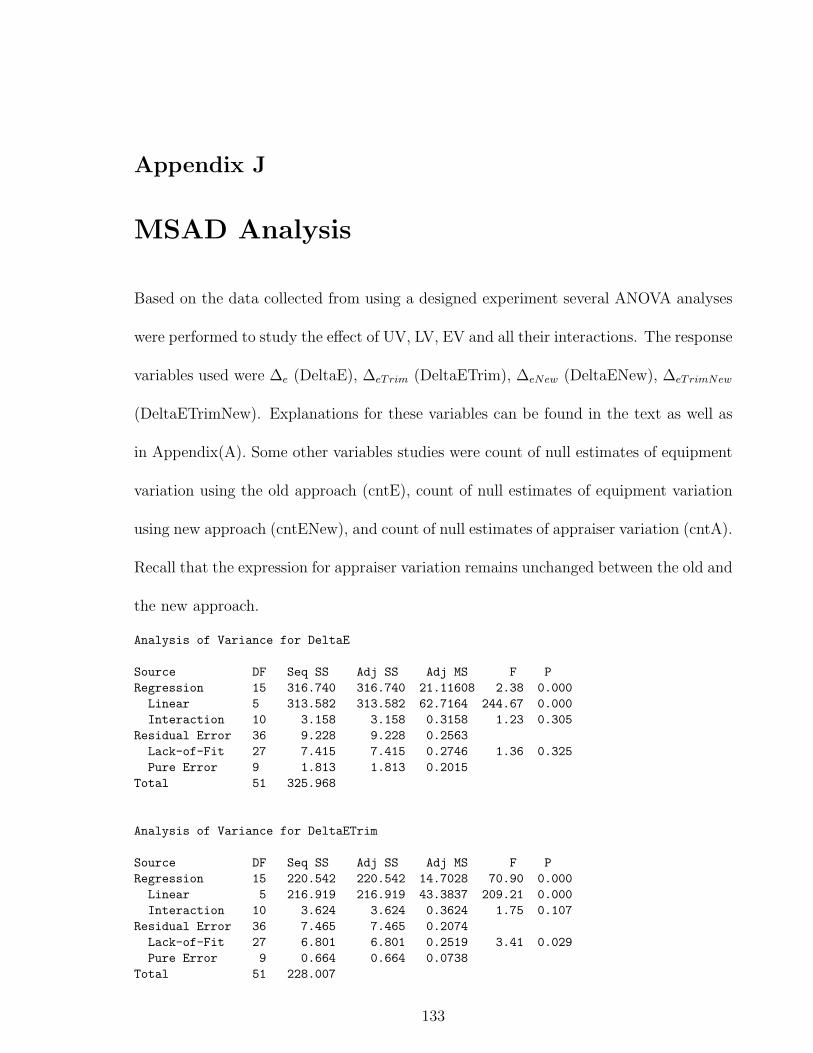
Appendix J
MSAD Analysis
Based on the data collected from using a designed experiment several ANOVA analyses
were performed to study the effect of UV, LV, EV and all their interactions. The response
variables used were ∆e (DeltaE), ∆eTrim (DeltaETrim), ∆eNew (DeltaENew), ∆eTrimNew
(DeltaETrimNew). Explanations for these variables can be found in the text as well as
in Appendix(A). Some other variables studies were count of null estimates of equipment
variation using the old approach (cntE), count of null estimates of equipment variation
using new approach (cntENew), and count of null estimates of appraiser variation (cntA).
Recall that the expression for appraiser variation remains unchanged between the old and
the new approach.
Analysis of Variance for DeltaE
Source DF Seq SS Adj SS Adj MS F PRegression 15 316.740 316.740 21.11608 2.38 0.000
Linear 5 313.582 313.582 62.7164 244.67 0.000Interaction 10 3.158 3.158 0.3158 1.23 0.305
Residual Error 36 9.228 9.228 0.2563Lack-of-Fit 27 7.415 7.415 0.2746 1.36 0.325Pure Error 9 1.813 1.813 0.2015
Total 51 325.968
Analysis of Variance for DeltaETrim
Source DF Seq SS Adj SS Adj MS F PRegression 15 220.542 220.542 14.7028 70.90 0.000
Linear 5 216.919 216.919 43.3837 209.21 0.000Interaction 10 3.624 3.624 0.3624 1.75 0.107
Residual Error 36 7.465 7.465 0.2074Lack-of-Fit 27 6.801 6.801 0.2519 3.41 0.029Pure Error 9 0.664 0.664 0.0738
Total 51 228.007
133
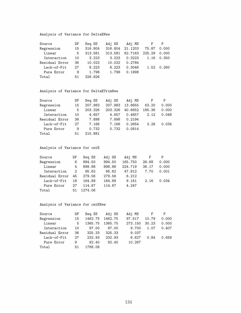
Analysis of Variance for DeltaENew
Source DF Seq SS Adj SS Adj MS F PRegression 15 316.804 316.804 21.1203 75.87 0.000
Linear 5 313.581 313.581 62.7163 225.29 0.000Interaction 10 3.223 3.223 0.3223 1.16 0.350
Residual Error 36 10.022 10.022 0.2784Lack-of-Fit 27 8.223 8.223 0.3046 1.52 0.260Pure Error 9 1.798 1.798 0.1998
Total 51 326.826
Analysis of Variance for DeltaETrimNew
Source DF Seq SS Adj SS Adj MS F PRegression 15 207.983 207.983 13.8655 63.20 0.000
Linear 5 203.326 203.326 40.6652 185.36 0.000Interaction 10 4.657 4.657 0.4657 2.12 0.048
Residual Error 36 7.898 7.898 0.2194Lack-of-Fit 27 7.166 7.166 0.2654 3.26 0.034Pure Error 9 0.732 0.732 0.0814
Total 51 215.881
Analysis of Variance for cntE
Source DF Seq SS Adj SS Adj MS F PRegression 6 994.50 994.50 165.750 26.68 0.000
Linear 4 898.88 898.88 224.719 36.17 0.000Interaction 2 95.62 95.62 47.812 7.70 0.001
Residual Error 45 279.56 279.56 6.212Lack-of-Fit 18 164.89 164.89 9.161 2.16 0.034Pure Error 27 114.67 114.67 4.247
Total 51 1274.06
Analysis of Variance for cntENew
Source DF Seq SS Adj SS Adj MS F PRegression 15 1462.75 1462.75 97.517 10.79 0.000
Linear 5 1365.75 1365.75 273.150 30.23 0.000Interaction 10 97.00 97.00 9.700 1.07 0.407
Residual Error 36 325.33 325.33 9.037Lack-of-Fit 27 232.93 232.93 8.627 0.84 0.659Pure Error 9 92.40 92.40 10.267
Total 51 1788.08
134
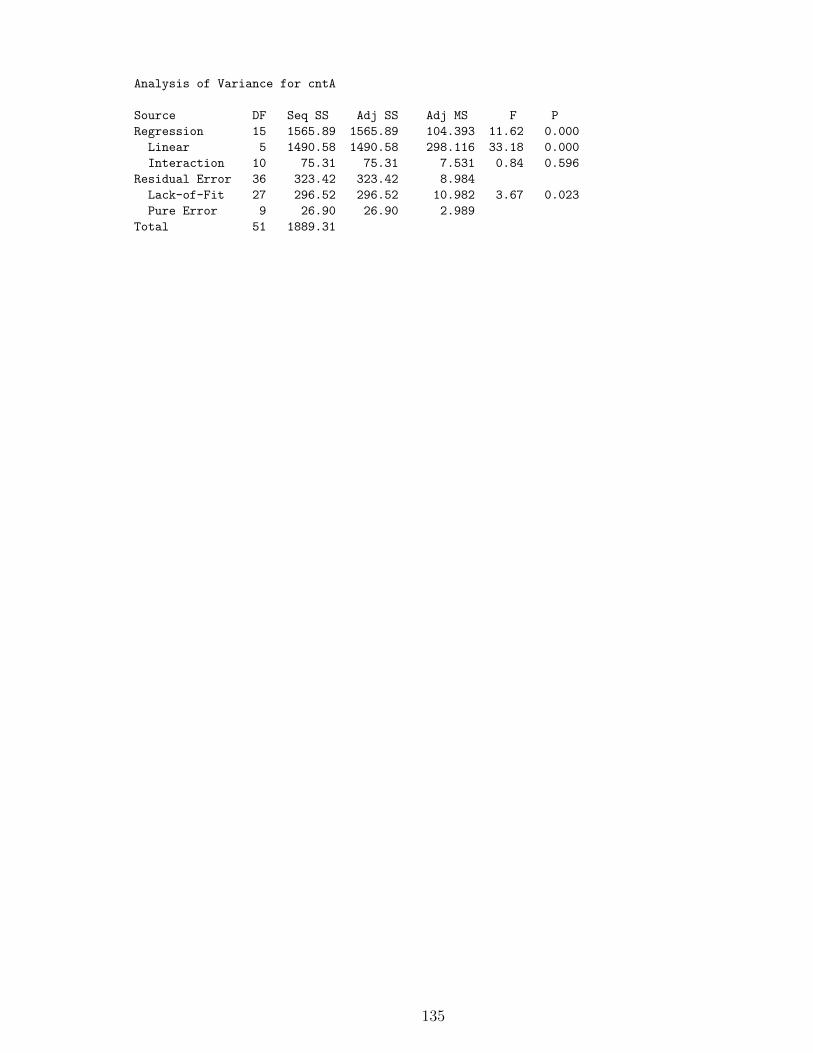
Analysis of Variance for cntA
Source DF Seq SS Adj SS Adj MS F PRegression 15 1565.89 1565.89 104.393 11.62 0.000
Linear 5 1490.58 1490.58 298.116 33.18 0.000Interaction 10 75.31 75.31 7.531 0.84 0.596
Residual Error 36 323.42 323.42 8.984Lack-of-Fit 27 296.52 296.52 10.982 3.67 0.023Pure Error 9 26.90 26.90 2.989
Total 51 1889.31
135
References
Ackermann, C. S. (1993). “Evaluating Destructive Measurements Using Gage R&R”. InIEEE/SEMI Advanced Semiconductor Manufacturing Conference.
AIAG (1996). Measurement System Analysis Reference Manual. Detroit, MI:AutomotiveIndustry Action Group.
AIAG (2003). Measurement System Analysis Reference Manual. Detroit, MI:AutomotiveIndustry Action Group.
ASQ Chemical and Process Industries Division (2001). Trusting measurement results inchemical and process industries. Milwaukee, WI:ASQ Quality Press.
Barrentine, L. B. (1991). Concepts for R&R Studies. Milwaukee, WI: ASQC QualityPress.
Bergeret, F.; Maubert, S.; Sourd, P.; and Puel, F. (2001). “Improving and applyingdestructive gauge capability”. Quality Engineering, 14(1), pp. 59–66.
Burdick, R. K.; Allen, A. E.; and Larsen, G. A. (2002). “Comparing variability of twomeasurement processes using R&R studies”. Journal of Quality Technology, 34(1), pp.97–105.
Burdick, R. K.; Borror, C. M.; and Montgomery, D. C. (2003). “A review of methods formeasurement systems capability analysis”. Journal of Quality Technology, 35(4), pp.342–354.
Christensen, R. (2002). Plane Answers to Comples Question: The Theory fo LinearModels. New York, NY: Springer.
Dolezal, K. K.; Burdick, R. K.; and Birch, N. J. (1998). “Analysis of a two-factor R&Rstudy with fixed operators”. Journal of Quality Technology, 30(2), pp. 163–170.
Duncan, A. J. (1974). Quality Control and Industrial Statistics. Homewood, IL: RichardD. Irwin, Inc.
Eagle, A. R. (1954). “A method for handling errors in testing and measuring”. IndustrialQuality Control.
Elam, M. E. (2001). Investigation, extension, and generalization of a methodology fortwo stage short run variables control charting. PhD thesis, Oklahoma State University.
Graybill, F. A. (1983). Matrices with applications in statistics. United States: DuxburyThomson Learning.
Grubbs, F. E. (1948). “On estimating precision of measuring instruments and productvariability”. Journal of American Statistics Association, 43, pp. 243–264.
136
Hahn, G. J. and Nelson, W. (1970). “A problem in the statistical comparison of measuringdevices”. Technometrics, 12(1), pp. 95–102.
John, P. (1994). Alternative models for gauge studies. SEMATECH report 93081755A-TR.
Kolarik, W. J. (1995). Creating Quality. New York: McGraw-Hill.
Kuehl, R. O. (2000). Design of experiments: statistical principles of research design andanalysis. New York: Duxbury Press.
Mitchell, T.; Hegemann, V.; and Liu, K. (1997). “GRR Methodology for Destructive Test-ing and Quantitative Assessment of Gauge Capability for One-Side Specifications”. InCzitrom, V. and Spagon, P. D., editors, Statistical Case Studies for Industrial ProcessImprovement, pages 47–59. Philadelphia:SIAM.
Montgomery, D. C. (1996). Introduction to statistical quality control. New York: JohnWiley & Sons, 3rd edition.
Montgomery, D. C. (2001). Design and analysis of experiments. New York: John Wiley& Sons, 5th edition.
Montgomery, D. C. and Runger, G. C. (1994a). “Gauge Capability Analsysi and DesignedExperiments. Part I: Basic Methods”. Quality Engineering, 6(1), pp. 115–135.
Montgomery, D. C. and Runger, G. C. (1994b). “Gauge Capability Analysis and De-signed Experiments. Part II: Experimental Design Models and variance componentestimation”. Quality Engineering, 6(2), pp. 289–305.
Morchower, N. D. (1999). “Two-location gauge evaluation”. Quality Progress, pages79–86.
Nunes, J. and Cherekdjian, S. (1995). “Reduction of measurement system variation usingthe Discrimination Ratio”. Nuclear Instruments and Methods in Physics Research B,96(1-2), pp. 118–122.
Patnaik, P. B. (1949). “The Use of Mean Range as an Estimator of Variance in StatisticalTests”. Biometrika, 37, pp. 78–87.
Potter, R. W. (1990). “Measurement system capability analysis”. In IEEE/SEMI Ad-vanced Semiconductor Manufacturing Conference.
Spiers, B. (1989). “Analysis of Destructive Measurement Systems”. ASQC QualityCongress Transactions, 43, pp. 22–27.
Vardeman, S. B. and VanValkenburg, E. S. (1999). “Two-Way Random-Effects Analysesand Gauge R&R Studies”. Technometrics, 41, pp. 202–211.
Walpole, R. E. and Myers, R. H. (1985). Probability and statistics for engineers andscientists. New York: McMillan, 3rd edition.
Wheeler, D. J. (1991). “Evaluating the Measurement Process When the Testing is De-structive”. In Presented at TAPPI conference, Nashville, TN.
137

Wheeler, D. J. (1992). “Problems with gauge R&R studies”. In 46th ASQC QualityCongress Transactions, Nashville, TN, pages 179–185.
Wheeler, D. J. and Lyday, R. W. (1984). Evaluating the Measurement Process. Knoxville,TN: SPC Press, Inc.
138

VITA
Mukul PatkiCandidate for the Degree of
Doctor of Philosophy
Thesis: Investigation, Improvement and Extension of Techniquesfor Measurement System Analysis
Major Field: Industrial Engineering & Management
Biographical:
Personal Data : Born in Durg, Madhya Pradesh, India, January 25, 1974,son of Suresh D. Patki and Archana S. Patki
Education : Graduated from high school in 1992; received a Bachelor’sdegree in Mechanical Engineering from Barkatullah University, Bhopal,India in June 1997; received a Master’s degree in Industrial Engineeringand Management from Oklahoma State University, Stillwater, OK inMay 2000; completed requirements for the Doctor of Philosophy degreeat Oklahoma State University in December 2005.
Experience : Maintenance and Operations Engineer, Indophil Textile Mills,Philippines (January 1998 – June 1998);Graduate Research Assistant, School of Industrial Engineering and Man-agement, Oklahoma State University (January 1999 – May 2000);Software Consultant, Information Sciences Corporation, Washington,DC (May 2000 – August 2000);Consultant, IBM TJ Watson Research Center, Yorktown Heights, NY(August 2000 – August 2001);Graduate Teaching/Research Assistant, School of Industrial Engineer-ing and Management, Oklahoma State University (August 2002 – May2005);Research Scientist, Knowledge Based Systems Inc., College Station, TX(June 2005 – current).
Honors : Material Handling Education Foundation Scholarship Award, Spring2003, Spring 2004; IEM Outstanding Teaching Assistant Award, Spring2004; Alpha Pi Mu invited member, Spring 1999;
Professional Membership : ASQ, INFORMS, IIE, SISO.
Name: Mukul Patki Date: December, 2005Institution: Oklahoma State University Location: Stillwater, OKTitle of Study: Investigation, Improvement, and Extension of Techniques
for Measurement System AnalysisPages of Study: 138 Candidate for the degree of Doctor of Philosophy
Purpose and scope of study: Critical manufacturing decisions are made based ondata obtained by randomly sampling production units. The effectiveness of these deci-sions depends on the accuracy of the data, which in turn depends on the accuracy andprecision of the measurement system. A measurement system is comprised of two primarycomponents - equipment or measuring devices and appraisers or personnel who use thesedevices. Each component adds to the variability of the data. The process of analyzingthis variation and estimating the contribution of various components of the measurementsystem toward this variation is known as measurement system analysis (MSA).
Automotive Industry Action Group (AIAG) has been at the forefront of MSAresearch. Through this dissertation, (i) improvements have been made in some of theexisting estimates of variance components (part variation); (ii) new variance componentshave been identified and quantified (within-appraiser variation); (iii) new approacheshave been suggested (using multiple measuring devices); (iv) the estimates of variancecomponents when measurement is destructive have been improved and adapted for chemi-cal and process industries; and (v) various measurement system acceptability criteria havebeen identified and their relative merits and demerits have been evaluated under varyingprocess capability conditions. Monte-Carlo simulation is used to verify the techniquesdeveloped as a part of this research.
Research contributions and conclusions: Within-appraiser variation is found tobe confounded with equipment variation. Lower bound for the former and upper boundfor the latter are estimated using two different approaches. The use of multiple equip-ment in the MSA study allows the estimation of variation among equipment which can bea significant component of the observed variation, and yet, is ignored in the current stateof MSA. The traditional estimate of part-to-part variation is corrected. Concurrent eval-uation of various measurement system acceptability criteria revealed that some of theseare in conflict with each other. Guidelines for the use of these criteria are developed.The difference between two such criteria—discrimination ratio and number of distinctcategories, are outlined. The current MSA approach for destructive testing scenarios issignificantly improved and new estimates for measurement variation are derived.
All simulation tests were done on a MATLAB-based software developed as part ofthis research. This software allows the simulation and analysis of various measurementsystems under widely varying conditions.
Advisor’s Approval: Dr. Kenneth Case