inverse modeling and uncertainty quantification of ... · the “adaptive anova-based probabilistic...
TRANSCRIPT

INVERSE MODELING AND UNCERTAINTY QUANTIFICATION OF
NONLINEAR FLOW IN POROUS MEDIA MODELS
by
Weixuan Li
A Dissertation Presented to the
FACULTY OF THE USC GRADUATE SCHOOL
UNIVERSITY OF SOUTHERN CALIFORNIA
In Partial Fulfillment of the
Requirements for the Degree
DOCTOR OF PHILOSOPHY
(CIVIL ENGINEERING)
May 2014
Copyright 2014 Weixuan Li

Dedication
To my family
1

Acknowledgments
I would like to express my greatest appreciation to everyone who was with me during the
entire or part of my journey of Ph.D study.
I would like to thank my advisor, Professor Dongxiao Zhang, for his consistent guid-
ance, support and all the research resources and opportunities he introduced to me, with-
out which this dissertation would never have been accomplished.
I would like to thank the professors on my dissertation committee: Dr. Felipe de Barros,
Dr. Roger Ghanem and Dr. Behnam Jafarpour, as well as Dr. Erik Jonhson who served on
my qualifying exam committee, for their valuable suggestions and comments.
I would like to extend my sincere thanks to my mentors and collaborators out of USC.
They are Dr. Adedayo Oyerinde, Dr. David Stern and Dr. Xiao-hui Wu from ExxonMobil
upstream research company, Dr. Guang Lin and Dr. Bin Zheng from Pacific Northwest
National Laboratory.
I would like to thank the former and current fellow students and post-doctors in our
2

and other research groups at USC, Heli Bao, Dr. Haibin Chang, Dr. Parham Ghods, Dr.
Ziyi Huang, Dr. Hamid Reza Jahangiri, Woonhoe Kim, Dr. Heng Li, Qinzhuo Liao, Le
Lu, Dr. Liangsheng Shi, Charanraj Thimmisetty, Dr. Ramakrishna Tipireddy, Dr. Hamed
Haddad Zadegan, Dr. Lingzao Zeng, Ruda Zhang,..., not only for the discussions and
shared thoughts that inspired my research, but also for the friendships that made my life
through the PhD study so much easier.
Finally, I would like to thank my wife Jie Yang and everyone in my family, for your
endless and unconditional love.
I acknowledge financial supports provided by US National Science Foundation, China
Scholarship Council, and Sonny Astani Department of Civil and Environmental Engineer-
ing.
3

Contents
Dedication 1
Acknowledgments 2
List of Tables 7
List of Figures 8
Abstract 14
Chapter 1 Introduction 17
1.1 Subsurface Flow Simulations under Uncertainty . . . . . . . . . . . . . . . . 17
1.2 Uncertainty Reduction by Inverse Modeling . . . . . . . . . . . . . . . . . . 19
1.3 Inversion Approaches: Dealing with Nonlinearity . . . . . . . . . . . . . . . 23
1.4 Objective and Scope . . . . . . . . . . . . . . . . . . . . . . . . . . . . . . . . . 35
Chapter 2 Bayesian Inversion 37
Chapter 3 Nonlinear Kalman Filter Approaches 41
3.1 Kalman Filter and its Nonlinear Variants . . . . . . . . . . . . . . . . . . . . . 42
3.1.1 Kalman Filter . . . . . . . . . . . . . . . . . . . . . . . . . . . . . . . . 42
3.1.2 Extended Kalman Filter . . . . . . . . . . . . . . . . . . . . . . . . . . 44
3.1.3 Ensemble Kalman Filter . . . . . . . . . . . . . . . . . . . . . . . . . . 45
3.1.4 Probabilistic Collocation Kalman Filter . . . . . . . . . . . . . . . . . 46
3.2 Adaptive ANOVA-based PCKF . . . . . . . . . . . . . . . . . . . . . . . . . . 49
3.2.1 PCE Approximation based on ANOVA Decomposition . . . . . . . . 50
3.2.2 Adaptive Selection of ANOVA Components . . . . . . . . . . . . . . 56
3.2.3 Additional Discussions on Implementation . . . . . . . . . . . . . . . 62
4

3.2.4 Summary of Adaptive ANOVA-based PCKF Algorithm . . . . . . . 65
3.3 Illustrative Examples . . . . . . . . . . . . . . . . . . . . . . . . . . . . . . . . 67
3.3.1 Problem 1: Saturated Water Flow in a Heterogeneous Aquifer . . . . 67
3.3.2 Problem 2: Waterflooding of a Petroleum Reservoir . . . . . . . . . . 81
3.4 Discussions . . . . . . . . . . . . . . . . . . . . . . . . . . . . . . . . . . . . . 90
Chapter 4 Adaptive Sampling via GP-based Surrogates 92
4.1 Sampling Methods . . . . . . . . . . . . . . . . . . . . . . . . . . . . . . . . . 93
4.1.1 Markov Chain Monte Carlo . . . . . . . . . . . . . . . . . . . . . . . . 93
4.1.2 Importance Sampling . . . . . . . . . . . . . . . . . . . . . . . . . . . 95
4.1.3 Simulated Annealing . . . . . . . . . . . . . . . . . . . . . . . . . . . . 96
4.2 Gaussian Process-based Surrogates . . . . . . . . . . . . . . . . . . . . . . . . 98
4.2.1 Basic Idea . . . . . . . . . . . . . . . . . . . . . . . . . . . . . . . . . . 98
4.2.2 Selection of Mean and Covariance functions . . . . . . . . . . . . . . 105
4.2.3 Models with Multiple Output Variables . . . . . . . . . . . . . . . . . 108
4.3 Adaptive Re-sampling and Refinement Algorithm . . . . . . . . . . . . . . . 109
4.3.1 Initialization . . . . . . . . . . . . . . . . . . . . . . . . . . . . . . . . . 110
4.3.2 Re-sampling via GP-based Surrogate . . . . . . . . . . . . . . . . . . 110
4.3.3 Refinement of Surrogate Models . . . . . . . . . . . . . . . . . . . . . 112
4.3.4 Summary of Work Flow . . . . . . . . . . . . . . . . . . . . . . . . . . 114
4.4 Illustrative Examples . . . . . . . . . . . . . . . . . . . . . . . . . . . . . . . . 116
4.4.1 Problem 3: Test on an Algebraic Function . . . . . . . . . . . . . . . . 116
4.4.2 Problem 4: I-C Fault Model . . . . . . . . . . . . . . . . . . . . . . . . 121
4.4.3 Problem 5: Solute Transport with Groundwater . . . . . . . . . . . . 129
4.5 Discussions . . . . . . . . . . . . . . . . . . . . . . . . . . . . . . . . . . . . . 142
Chapter 5 Conclusion, Discussions, and Future Work 143
5.1 Conclusion . . . . . . . . . . . . . . . . . . . . . . . . . . . . . . . . . . . . . . 143
5.2 Discussions . . . . . . . . . . . . . . . . . . . . . . . . . . . . . . . . . . . . . 144
5.3 Future work . . . . . . . . . . . . . . . . . . . . . . . . . . . . . . . . . . . . . 145
5

Nomenclature 147
Abbreviations 150
Bibliography 151
6

List of Tables
3.1 List of case studies of Problem 1 with different prior variances and observa-
tion errors. . . . . . . . . . . . . . . . . . . . . . . . . . . . . . . . . . . . . . . 68
3.2 Number of PCE basis functions selected by three criteria (average number
of 10 data assimilation loops). . . . . . . . . . . . . . . . . . . . . . . . . . . . 78
4.1 List of case studies of Problem 5 with different parameter and observation
settings. . . . . . . . . . . . . . . . . . . . . . . . . . . . . . . . . . . . . . . . . 130
7

List of Figures
1.1 Work flow of forward and inverse modelings. . . . . . . . . . . . . . . . . . . 20
3.1 First order ANOVA components’ variances of model output in Problem 1
(h|x=0.05). . . . . . . . . . . . . . . . . . . . . . . . . . . . . . . . . . . . . . . . 69
3.2 Adaptive selection of PCE bases using three criteria for case 1, Problem 1
(ǫ = 0.05). . . . . . . . . . . . . . . . . . . . . . . . . . . . . . . . . . . . . . . . 70
3.3 Uncertainty quantification of model output h(x) and calibration to observa-
tions, Adaptive PCKF, criterion 3. . . . . . . . . . . . . . . . . . . . . . . . . . 71
3.4 Uncertainty quantification of model parameter Y (x), Adaptive PCKF, crite-
rion3. . . . . . . . . . . . . . . . . . . . . . . . . . . . . . . . . . . . . . . . . . 72
3.5 Comparison of the parameter estimations given by EnKFs, non-adaptive
PCKFs and Adaptive PCKFs (Problem 1). . . . . . . . . . . . . . . . . . . . . 75
8

3.6 Efficiency comparison between EnKFs, non-adaptive PCKFs and Adaptive
PCKFs using H2 index (Case 1, Problem 1). . . . . . . . . . . . . . . . . . . . 76
3.7 Efficiency comparison between EnKFs, non-adaptive PCKFs and Adaptive
PCKFs using H2 index (Case 2, Problem 1). . . . . . . . . . . . . . . . . . . . 79
3.8 Efficiency comparison between EnKFs, non-adaptive PCKFs and Adaptive
PCKFs using H2 index (Case 3, Problem 1). . . . . . . . . . . . . . . . . . . . 80
3.9 Oil recovery from a reservoir by waterflooding. . . . . . . . . . . . . . . . . . 83
3.10 Simulated production history with uncertainty quantification, before model
calibration (Problem 2). . . . . . . . . . . . . . . . . . . . . . . . . . . . . . . . 85
3.11 Simulated production history with uncertainty quantification, after model
calibration (Problem 2). . . . . . . . . . . . . . . . . . . . . . . . . . . . . . . . 86
3.12 Estimated mean and standard deviation of log permeability by adaptive
ANOVA-based PCKF (Problem 2). . . . . . . . . . . . . . . . . . . . . . . . . 87
3.13 Number of PCE bases adaptively selected by criterion 3 (problem 2). . . . . 88
3.14 Efficiency comparison between EnKFs, non-adaptive PCKFs and Adaptive
PCKFs using H2 index (problem 2). . . . . . . . . . . . . . . . . . . . . . . . . 89
4.1 An example of a pdf at different temperatures. . . . . . . . . . . . . . . . . . 97
9

4.2 Comparison between the true and GP-based surrogate model responses,
and their corresponding posterior distributions of the model parameter given
an observation of the model output. The surrogate and its error estimation
are represented by a Gaussian process conditioned to model evaluations at
three base points. . . . . . . . . . . . . . . . . . . . . . . . . . . . . . . . . . . 102
4.3 Comparison between the true and GP-based surrogate model responses,
and their corresponding posterior distributions of the model parameter given
an observation of the model output. The surrogate and its error estimation
are represented by a Gaussian process conditioned to the model evaluations
at three initial base points and one refinement point. . . . . . . . . . . . . . . 103
4.4 Comparison between the true and mean response of the surrogate model,
and their corresponding posterior distributions of the model parameter given
an observation of the model output. The surrogate is built by a Gaussian
process conditioned to model evaluations at three base points. The surro-
gate error is not considered when computing the posterior distribution. . . 104
4.5 Four GP-based surrogates built on the same base points but with different
assumptions of the covariance function. . . . . . . . . . . . . . . . . . . . . . 107
10

4.6 Use a Gaussian mixture distribution as the proposal distribution for im-
portance sampling: an illustrative example. (a) 300 original sample points;
(b) clustering of the original sample points; (c) Gaussian mixture distribu-
tion fitted from the clusters; (d) 1000 new sample points proposed from the
Gaussian mixture distribution. . . . . . . . . . . . . . . . . . . . . . . . . . . 113
4.7 Mean and standard deviation of the GP-based surrogate built on 9 initial
base points (Problem 3). . . . . . . . . . . . . . . . . . . . . . . . . . . . . . . 117
4.8 Sample points obtained in different re-sampling and refinement loops (Prob-
lem 3). . . . . . . . . . . . . . . . . . . . . . . . . . . . . . . . . . . . . . . . . 119
4.9 Standard deviations of the surrogate errors in different refinement loops
(Problem 3). . . . . . . . . . . . . . . . . . . . . . . . . . . . . . . . . . . . . . 120
4.10 I-C Fault model (Carter et al., 2006), distances are measured in feet (Problem
4). . . . . . . . . . . . . . . . . . . . . . . . . . . . . . . . . . . . . . . . . . . . 122
4.11 Simulation results of the I-C Fault model based on the parameter points
sampled from prior distribution (Problem 4). . . . . . . . . . . . . . . . . . . 123
4.12 Comparison between original I-C Fault model responses and surrogate re-
sponses evaluated at three randomly selected parameter points. The re-
sponses of the GP-based surrogate are shown with error estimation (mean
+/- 2 standard deviations), (Problem 4). . . . . . . . . . . . . . . . . . . . . . 125
11

4.13 Sample from the posterior distribution of the I-C Fault model parameters
via the GP-based surrogate built on 40 initial base points (Problem 4). . . . . 126
4.14 Sample from the posterior distribution of the I-C Fault model parameters
via the GP-based surrogate built on 40 initial and 45 refinement base points
(Problem 4). . . . . . . . . . . . . . . . . . . . . . . . . . . . . . . . . . . . . . 126
4.15 Simulation results of the I-C Fault model based on the parameter points
sampled from posterior distributions obtained using the final GP-based sur-
rogate (Problem 4). . . . . . . . . . . . . . . . . . . . . . . . . . . . . . . . . . 127
4.16 Sample from the posterior distribution of the I-C Fault model parameters
using a large number of Monte Carlo simulations (Problem 4). . . . . . . . . 127
4.17 Predictions of cumulative oil production for the next 7 years after the first
three years of observed production history. Simulations are based on 1) sam-
ple parameter points from the prior distribution and 2) sample parameter
points obtained from the posterior distribution using G-P based surrogate
(Problem 4). . . . . . . . . . . . . . . . . . . . . . . . . . . . . . . . . . . . . . 128
4.18 Schematic representation of the solute transport model (Problem 5). . . . . . 129
4.19 Concentration breakthrough curves at well obs2 simulated using prior sam-
ple points (Case 1, Problem 5). . . . . . . . . . . . . . . . . . . . . . . . . . . . 132
4.20 Estimated posterior distribution (Case 1, Problem 5); (a) posterior sample
points; (b-d) posterior histograms for each uncertain parameter. . . . . . . . 133
12

4.21 Concentration breakthrough curves at well obs2 simulated using posterior
sample points (Case 1, Problem 5). . . . . . . . . . . . . . . . . . . . . . . . . 134
4.22 Estimated posterior distribution (Case 2, Problem 5); (a) posterior sample
points; (b-d) posterior histograms for each uncertain parameter. . . . . . . . 136
4.23 Concentration breakthrough curves at wells obs1, obs2, obs3, simulated using
prior and posterior sample points (Case 2, Problem 5). . . . . . . . . . . . . 137
4.24 Estimated posterior histograms for each uncertain parameter (Case 3, Prob-
lem 5). . . . . . . . . . . . . . . . . . . . . . . . . . . . . . . . . . . . . . . . . 138
4.25 Concentration breakthrough curves at wells obs1-obs6, simulated using prior
and posterior sample points (Case 3, Problem 5). . . . . . . . . . . . . . . . . 139
4.26 Posterior histograms for each uncertain parameter estimated by sampling
via the true model (Case 3, Problem 5). . . . . . . . . . . . . . . . . . . . . . . 141
13
Abstract
When using computer models to predict flow in porous media, it is necessary to set pa-
rameter values that correctly characterize the geological properties like permeability and
porosity. Besides direct measurements of these geological properties, which may be ex-
pensive and difficult, parameter values could be obtained from inverse modeling which
calibrates the model to any available observations on flow behaviors such as pressure, sat-
uration and well production rates. A typical inverse problem has non-unique solutions
because the information contained in the observations is usually insufficient to identify all
uncertain parameters. Finding a single solution to the inverse problem that well matches
all observations does not guarantee the correct representation of the real geological sys-
tem. In order to capture multiple solutions and quantify remaining uncertainty we solve
an inverse problem from a probabilistic point of view: seek the posterior distribution of
parameters given the observations using Bayes’ theorem. In the situation where the model
is nonlinear, which is often the case of subsurface flow problems, the posterior distribu-
tion cannot be analytically derived. Instead we implement numerical algorithms to find
approximate results. The key to running an inversion algorithm is to understand how the
14

model input (parameters) and model output (simulation results) are related to each other.
For complex models where direct derivation is difficult this task can be done by running a
large number of trial simulations with different parameter values. These algorithms work
well for simple small scale models but are prohibitively expensive to apply to subsurface
flow models since each single run may take a long time and we do not have unlimited time
and resource to run the trial simulations.
The main contribution of this research is the development and test of two approaches—
the “adaptive ANOVA-based probabilistic collocation Kalman filter (PCKF)” and “adap-
tive sampling via Gaussian process (GP)-based surrogates”—for inverse modeling of non-
linear flow in porous media models. Both approaches fall into the category of probabilistic
inversion and have the capability to quantify remaining uncertainty. This study focuses
on computational efficiency, which is often the bottleneck of implementing inverse mod-
eling and uncertainty quantification (UQ) algorithms for nonlinear models. The selection
of proper inversion approach to be used is problem dependent. The “adaptive ANOVA-
based PCKF”, is a nonlinear variant of the classic Kalman filter approach, which estimates
the first two statistical moments, i.e., mean and covariance, of the posterior distribution.
It applies to the problems where the nonlinearity is mild and the posterior distribution is
approximately Gaussian. The main idea is to represent and propagate uncertainty with
a proper polynomial chaos expansion (PCE) that is adaptively selected for the specific
problem. The second method is more general and deals with stronger nonlinearity and
non-Gaussian, even multi-modal, posterior distributions. Sampling approaches usually
cost even more computational effort comparing with Kalman filter methods. But in our al-
15

gorithm, the efficiency is greatly enhanced by the following four features: a GP surrogate
for simulation acceleration, an adjustment of the posterior considering surrogate error, an
importance sampler using Gaussian mixture proposal distribution, and an adaptive re-
finement scheme. The developed approaches are demonstrated and tested with different
models.
16

Chapter 1
Introduction
1.1 Subsurface Flow Simulations under Uncertainty
Numerical models are powerful tools to simulate the fluid flow through porous media. It
has many research and industrial applications in the areas such as oil and gas recovery,
groundwater management, pollutant transport assessment, and geological sequestration
of greenhouse gases. After decades of development, the state-of-the-art simulators are now
capable of solving coupled partial differential equations governing the complex subsurface
multiphase flow system within a practically large spatial and temporal domain. However,
despite the advances in numerical approaches and computing capabilities, researchers and
engineers still find it challenging to make accurate predictions for real practical problems.
One of the biggest difficulties is to assign the correct values to the model parameters when
they are subject to uncertainty.
17

Chapter 1. Introduction
Subsurface flow behaviors depend on the geological properties such as permeability,
porosity, fault transmissibility, etc. Thus it is necessary for a modeler to find the parameter
values that correctly characterize these properties. But this is not an easy task. The geolog-
ical properties are location dependent and often reveal a strong heterogeneity. In addition
precise and comprehensive measurements are difficult and usually very expensive. These
facts prevent modelers from obtaining the complete information of these properties. In
addition to the geological properties, uncertain parameters also may arise from our in-
complete knowledge about boundary and initial conditions, e.g., the rate of recharge to
an aquifer, or the initial position of the oil-water contact in a petroleum reservoir. These
uncertain parameters could be a major contributor to the discrepancy between simulation
results and reality.
To address this problem one could consider all possible parameter values that are con-
sistent with the available measurement data and other pre-given geological descriptions
such as experts’ opinion. Mathematically, the model parameters are expressed as random
variables (or stochastic processes if the parameters are location/time dependent), which
are characterized by the corresponding probability distributions. For models with stochas-
tic parameters, the model output also becomes random. To make reliable prediction one
needs to study how the parameter uncertainty propagates through model and affects the
simulation results. For example, we may give an estimated error bound for the simulated
output. This process is referred to as “(forward) UQ”. The studies regarding the stochas-
tic flow in porous media and uncertainty quantification are summarized in the books by
Zhang (2001), Rubin (2003), and Dagan and Neuman (2005).
18

Chapter 1. Introduction
1.2 Uncertainty Reduction by Inverse Modeling
If we hope to reduce the uncertainty and make more accurate predictions, we need to
gather more information about the parameters. Besides direct measurements of the input
parameters, the field measurement/observation of flow behaviors is another important
source of information which helps us improve the estimation of parameters as well as the
credibility of predictions about other output variables. The idea is straightforward: only
the parameter values from which the simulation results match the observed field data
should be trusted and used for prediction. Examples of such field data include the water
head observations in a groundwater problem, the concentration measurements in a pollu-
tant transport problem, the bottom-hole pressure and production rates recorded at wells
in an oil recovery problem, etc. The work of calibrating model parameters to field data is
known as “data assimilation”. Since this process infers the input variables (parameters)
from the observations on some of the output variables, we also call it “inverse modeling”.
Previous studies on inverse modeling of flow in porous media problems are seen in the
review papers by Yeh (1986) and Oliver and Chen (2011). The calibrated parameters are
then used to make predictions to other output variables in a forward modeling procedure.
The work flow of forward and inverse modelings is illustrated in Fig. 1.1.
Solving inverse modeling problems is challenging, especially when one has multiple
parameters to estimate and multiple field observations to match. Usually, what we have at
hand is a simulator that solves the deterministic forward problem. The forward problem
is well defined, i.e. for a deterministic input submitted to the simulator we get a unique
19

Chapter 1. Introduction
Measurable output variables!!
Output variables to be predicted!
Inverse modeling!
Forward modeling!
Uncertain input parameters!!
Known input parameters!
• Flow behaviors
• Pressure
• Satura2on
• Concentra2on
• Flow rate
…
• Geological proper2es
• Ini2al condi2ons
• Boundary condi2ons
…
Figure 1.1: Work flow of forward and inverse modelings.
output returned by the simulator. In contrast, the simulator does not generate a model
“input” with a given “output”. In fact, one should note that an inverse problem is usu-
ally ill-posed and has non-unique solutions. This means that for a single deterministic
observed value of the output one may find multiple corresponding input values that all
give a match to the output value. Essentially, this is because the information contained
in the data measurement is insufficient to determine all the uncertain model parameters.
Specific reasons causing non-unique solutions include the following ones.
First, in most inverse problems we have less number of independent observations than
the independent uncertain parameters. Like solving equations, this implies that we do
not have enough constraints to determine all the parameters, and there are different com-
binations of parameter values that all result in a match to the observations. The second
typical reason is the nonlinear input-output relationship. Most subsurface flow models
are nonlinear and this may cause non-unique solutions even if the model parameters are
constrained by the same number of observations. The third reason is acceptable mismatch.
20

Chapter 1. Introduction
Besides inaccurate model parameters, there are other causes of the discrepancy between
real field measurements and simulation results. For instance, measurement errors associ-
ated with observations. In addition, the model used in the simulation could be imperfect
and results in a modeling error comparing with the real physical process to be simulated.
These errors contribute to the mismatch between the simulation result and the observation
made in the real world even if we have accurate parameter values. Considering this fact,
one should keep all those parameter points if their corresponding mismatch is within an
acceptable error range, rather than requiring a strict zero mismatch.
Approaches solving inverse problems can be roughly divided into two categories: de-
terministic inversion and probabilistic inversion. In deterministic inversion approaches,
we seek a single point in the parameter space that results in the best match to the ob-
served data. This is done by searching for the minimum point of an objective function
which quantifies the difference between the simulation results and the observations. The
minimization could be implemented by typical numerical optimization algorithms such
as gradient-based approaches or genetic algorithms. Once an optimal parameter point is
obtained, it is then used for predicting quantities of our interest. For ill-posed inverse
problems with non-unique solutions, a regularized term that reflects the modeler’s prior
preference may be added to the objective function to help identify a single solution.
Non-unique solutions of an inverse problem indicate that the uncertainty associated
with model parameters is not eliminated by the observations, but usually only greatly
reduced. For example, the variances of uncertain parameters become smaller but not neg-
ligible.
21
Chapter 1. Introduction
In this situation, the single solution provided by the deterministic inversion approach,
which omits the remaining uncertainty, does not lead to a reliable prediction of future,
because such a solution could deviate from reality even it nicely matches all the field data.
Instead, we prefer to keep all possible scenarios in the solution of the inverse problem,
which brings the idea of probabilistic inversion approaches. With multiple solutions one
can re-assess the remaining uncertainty in the parameters and the simulation results after
the data assimilation. In this sense, we also call the probabilistic inverse modeling “inverse
uncertainty quantification”.
In order to capture multiple solutions and quantify the remaining parameter uncer-
tainty we formulate an inverse modeling problem from a probabilistic point of view, rather
than the optimization approaches talked previously. Tarantola (2005) proposed a method
of “combination of states of information” to quantify parameter uncertainty. In our study
we adopt the more widely used approach of Bayesian inversion. See the book by Kai-
pio and Somersalo (2006) and the book by Oliver et al. (2008) for reference. In Bayesian
probabilistic inversion approaches different solutions are represented by the “posterior
probability distribution” of the model parameters given the observations. By the Bayes’
theorem the posterior distribution is calculated from the pre-specified prior distribution
as well as the likelihood function. While the likelihood function represents the informa-
tion about model parameters obtained from observations, the prior distribution reflects
the information from all other sources, e.g., a physically meaningful range constraining
the parameter value, experts’ opinions, or direct measurements. Although the posterior
distribution provides the complete information of the remaining uncertainty associated
22

Chapter 1. Introduction
with model parameters, it in general cannot be analytically derived except for a few spe-
cial cases, e.g., linear models with Gaussian pdfs, or models where the parameters can
take only finite number of discrete values. Often we rely on numerical algorithms to find
approximate representations of the posterior distributions. In most of the current avail-
able numerical algorithms solving inverse modeling problems, the key procedure is to
make a large number of trial model simulations with different parameter values, which
are used to detect the nonlinear input-output relationship in a model. While these algo-
rithms work well for some other models they cannot be simply applied to subsurface flow
models because each single simulation may take a long time and running a large number
of simulations is impractical.
1.3 Inversion Approaches: Dealing with Nonlinearity
One special case in which the posterior distribution can be analytically derived is linear
models with the prior density of parameters and measurement errors both normally dis-
tributed. Under these conditions, the posterior distribution of model parameters is also
normal and hence fully characterized by its first two statistical moments, mean and co-
variance. The classic algorithm to solve such kind of inverse problems is Kalman filter
(Kalman, 1960). In addition, the Kalman filter is usually implemented in a recursive man-
ner. Suppose the data (measurements) come available as a time sequence. For each node
on this data sequence, we solve an inverse modeling problem. The posterior mean and
covariance computed from the previous step serve as the prior for the next step. When-
23

Chapter 1. Introduction
ever new data are collected, the parameters are updated correspondingly. This process is
known as sequential data assimilation.
For nonlinear systems, the posterior distribution generally is non-Gaussian, regardless
of whether or not the prior density and observation error are Gaussian. As long as the
nonlinearity is not strong, the Kalman filter still yields a good approximate solution of the
posterior mean and covariance. The key step in implementing the Kalman filter is to com-
pute the “Kalman gain,” which requires knowledge of the covariance of the (prior) joint
distribution of model parameters and output variables. While this covariance is easily
computed for linear systems, extra computational effort is necessary to estimate it for non-
linear models. Indeed, a forward UQ problem must be solved to study how the parametric
uncertainty propagates through the nonlinear system to affect the output quantities. This
becomes the main difficulty and computational overhead in extending the Kalman filter to
nonlinear models.
A straightforward way to apply Kalman filter to nonlinear models is to implement a
first-order linearization to the model around its prior mean. This method is known as “ex-
tended Kalman filter (EKF)” (Anderson and Moore, 1979). One of the disadvantages of
EKF is its instability when the prior estimation is far away from the true state. Moreover,
EKF requires computing the Jacobian matrix, i.e., the partial derivatives of the model out-
puts with respect to the model parameters. This could be extremely costly for models with
a large number of parameters.
The ensemble Kalman filter (EnKF), a relatively new nonlinear variant of the Kalman
filter, represents and propagates uncertainty using the Monte Carlo method (Evensen,
24

Chapter 1. Introduction
1994, 2009). First, a number of realizations (an ensemble) of model parameters are ran-
domly sampled from the prior distribution. Then, for each realization, a simulation is run
to predict the corresponding realization of model outputs, and the required covariance is
estimated from the joint ensemble. Finally, each realization is updated by the Kalman fil-
ter to form a new ensemble that represents the posterior distribution of model parameters.
Due to the simplicity in its implementation, EnKF has gained great popularity within the
past two decades. Since its invention, EnKF has been applied to many different research
fields including the modeling of flow in porous media (Chen and Zhang, 2006; Aanon-
sen et al., 2009) and has demonstrated great effectiveness. Evensen (2003) has provided
a review of the development and applications of EnKF. However, like all Monte Carlo
approaches, EnKF’s accuracy relies on a sufficiently large ensemble, which causes an enor-
mous computational burden for large-scale computational models.
An alternative to the Monte Carlo method for studying uncertainty propagation is the
PCE. In this approach, the random quantities under study are expanded using a polyno-
mial chaos basis, which are the orthogonal polynomials with respect to a set of indepen-
dent random variable with known distributions (Wiener, 1938; Ghanem and Spanos, 2003;
Xiu and Karniadakis, 2003). Once the PCE representation is obtained, the statistical mo-
ments of our interest (e.g., mean and covariance of the random quantities) can be easily
computed from the coefficients in front of the polynomial chaos basis.
The key–and computationally demanding–step of implementing the PCE approach is
solving for the PCE coefficients. Among different methods available to tackle this prob-
lem, such as the stochastic Galerkin projection (Ghanem and Spanos, 2003) and regression
25

Chapter 1. Introduction
method (Isukapalli et al., 1998), the probabilistic collocation method (PCM) (Tatang et al.,
1997) is particularly convenient and effective. PCM constructs the PCE approximation
by interpolation, where the interpolation points are called “collocation points.” Similar to
Monte Carlo, PCM is a non-intrusive approach, which means it treats the model as a black
box and requires only repetitive evaluations of the model at the collocation points with a
deterministic simulator. To achieve high accuracy in estimating the statistical moments,
which by definition are integrals over the random space, the collocation points usually are
deployed the same way as the quadrature points used in numerical integration schemes,
such as Gauss quadrature points. For high-dimensional PCM, commonly used collocation
schemes include sparse grid and Stroud quadrature points (Xiu and Hesthaven, 2005). A
discussion regarding the selection of collocation points is given by Eldred and Burkardt
(2009). PCM was compared with the Monte Carlo method in previous studies and demon-
strated better efficiency in solving forward UQ problems for flow in porous media models
(Li and Zhang, 2007, 2009; Li et al., 2009; Lin and Tartakovsky, 2009).
Similar to the EnKF, which combines the Monte Carlo method with the Kalman filter,
the so-called “PCKF” or “polynomial chaos-based ensemble Kalman filter”, which com-
bines the PCE with the Kalman filter, was developed to solve inverse modeling problems
(Saad and Ghanem, 2009; Li and Xiu, 2009; Zeng and Zhang, 2010; Zeng et al., 2011; Li
et al., 2011). PCKF resembles EnKF in almost every aspect except that it uses the PCE to
represent uncertainty. While an EnKF user must decide on the size of the ensemble be-
fore running the algorithm, a PCKF user has to determine in advance the truncation of
the PCE, i.e., to select the basis functions to form the PCE approximation. The trade-off is
26

Chapter 1. Introduction
that keeping more PCE basis functions helps to capture uncertainty more accurately, but
it increases the computational cost. An ideal PCE should accurately represent the model
uncertainty but keep the number of basis functions as small as possible. Dealing with
this issue is particularly vital in solving high-dimensional problems (i.e., stochastic mod-
els with a large number of uncertain parameters) because the total number of PCE terms
can grow dramatically fast as the dimensionality increases.
A general guideline for choosing the PCE bases for PCKF was lack in previous re-
searches. In this study, we develop a new algorithm (Li et al., 2014) that adaptively se-
lects active PCE basis functions for uncertainty representation in different problems and
automatically adjusts the number of basis functions in different Kalman filter loops. We
construct the PCE based on adaptive functional analysis of variance (ANOVA) decompo-
sition. Functional ANOVA, also referred to as “high-dimensional model representation”
(HDMR), was shown as an effective dimensionality reduction method (Rabitz and Alis,
1999; Li et al., 2001)and was combined with PCE approximation to solve forward UQ prob-
lems (Foo and Karniadakis, 2010). Now, we extend this methodology toward solving in-
verse modeling problems. Because in many physical models the coupling effect of a large
number of input parameters on the model output can be reduced to the coupling effect of
only a few, functional ANOVA decomposition is able to approximate a high-dimensional
function with the summation of a set of low-dimensional functions, known as ANOVA
components. For different models, the components of the ANOVA decomposition may be
adaptively calculated following some adaptive criterion, which greatly reduces the com-
putational cost and improves efficiency (Ma and Zabaras, 2010; Yang et al., 2012). Once
27

Chapter 1. Introduction
an ANOVA decomposition is done, the ANOVA components (low-dimensional) can be
expanded with PCE, which is much less costly than expanding the original model (high-
dimensional).
Although the above mentioned Kalman filter’s variants have been shown working
well in many studies of nonlinear inverse problems, one should note that all these meth-
ods could fail for highly nonlinear models when the assumptions on which Kalman filter
is based are severely violated. Kalman filter only uses the first two statistical moments
(mean and covariance) to describe the joint distribution of the parameters and model out-
puts when solving inverse problems. The information contained in higher-order moments
is not seen by the algorithm. In an extreme case, it is possible that model input and output
are nonlinearly dependent with each other but statistically uncorrelated, i.e., their covari-
ance is zero. In this situation Kalman filter and its variants cannot infer input from the
observations of the output. Strong non-linearity also may lead to multimodal posterior
distributions in which situation only estimating the first two statistical moments simply
does not provide enough insight into the posterior.
To deal with strong nonlinearity and to characterize an arbitrary posterior density, we
put down the Kalman filters and go back to solve the Bayesian inverse problem directly.
If the posterior density cannot be analytically derived, we could draw a sample of real-
izations to represent it, which is again the idea of Monte Carlo methods. (Note that in
EnKF the purpose of using Monte Carlo method is to estimate the required prior statistical
moments and the updated ensemble does not accurately represent the posterior distribu-
tion unless the model is indeed linear). Examples of Monte Carlo approaches include the
28

Chapter 1. Introduction
Particle filter (Gordon et al., 1993), the Markov chain Monte Carlo (MCMC) (Metropolis
et al., 1953; Hastings, 1970), etc. Implementing a typical Monte Carlo algorithm requires to
randomly sample a set of points in the parameter space according to the prior distribution.
For each parameter point the model is evaluated to generate the corresponding output
which is then compared with the field data. Only those parameter points that match the
field data are kept (following certain rules) to represent the posterior distribution. In many
cases, the probability that a randomly selected point hit the target is small. To have enough
points representing the posterior distribution one has to sample and evaluate an extremely
large number of parameter points. This makes Monte Carlo methods intractable for large
scale models which are time consuming to run.
A practical inversion algorithm is expected to keep the computational cost as low as
possible. One of the straightforward ideas to lessen the computational cost is to use sur-
rogate models. A surrogate (also called a meta-model, or a reduced order model in differ-
ent studies) is an approximation of the original true model that can be quickly evaluated.
With a surrogate replacing the original model, drawing a large enough sample becomes
affordable and hence makes Monte Carlo methods applicable. A good surrogate should
be both economical and accurate. Various types of surrogate models have been studied in
previous researches to approximate parameter-output relationships for objectives includ-
ing prediction, optimization, sensitivity analysis, uncertainty analysis and inverse model-
ing/calibration. Razavi et al. (2012) gave a review of the surrogate models used in the field
of water resources research, which are divided into two categories: statistical data-driven
models and lower-fidelity physically based surrogates. The construction of the first type of
29

Chapter 1. Introduction
surrogate models often requires a number of simulations of the original model at a group
of parameter points based on an experimental design scheme, from which a response sur-
face over the entire parameter space is then quickly generated using some technique. In
the context of inverse modeling, examples of such techniques include polynomial approx-
imations like the PCE (also known as “stochastic response surface” in some literature)
(Balakrishnan et al., 2003), radial basis functions interpolation (Bliznyuk et al., 2008), and
the neural network (Zou et al., 2009). Examples of the second category of surrogates in-
clude models built on coarser spatial and/or temporal grid size, simplified mathematical
equations or physical models.
In previous studies on surrogate-based sampling algorithms for inverse modeling, the
original models usually were simply replaced with selected surrogate models under the
assumption that the approximation error is negligible. However, surrogate accuracy is in-
deed a crucial issue. One needs to keep in mind that an inaccurate surrogate in a sampling
algorithm causes extra sampling error and results in a biased estimation of the parameters.
For example, a parameter point that matches the field data through the original model but
not through the inaccurate surrogate may be mistakenly ruled out of the sample. On the
other hand, a parameter point out of the true posterior distribution may be sampled if it
happens to fit the observations through the inaccurate surrogate.
To reduce such mistakes, we need an error estimation for the surrogate approximation.
Note that the approximation error, which is defined as the difference between the output
values given by the original model and the surrogate, is deterministic in the sense that re-
peated computational experiments with the same input parameter point would yield the
30

Chapter 1. Introduction
same output difference. However, in practice the output value of the original model is not
known without running simulations, so the approximation error at each parameter point
is generally uncertain and is expressed as a random variable. The accuracy of the surrogate
is measured by the spread, e.g., estimated standard deviation, of the approximation error.
This quantity indicates how reliable the surrogate is when we use it for inverse modeling.
With an error estimation of the surrogate, we can modify sampling algorithms accord-
ingly to avoid the above mentioned mistakes caused by inaccurate surrogate. Specifically,
we sample from an adjusted posterior distribution, which incorporate the estimation of
approximation error. When the surrogate is accurate, i.e., with a small approximation er-
ror, the modified sampling algorithm works almost the same way as sampling via the true
model response. However, a large estimated surrogate error would have an effect on the
sampling rule. The sampling algorithm should tolerate those parameter points that do not
match the observation but lead to a mismatch within a reasonable range considering the
estimated approximation error. The reason is that the mismatch could be induced by either
an incorrect parameter point or the surrogate error. Before we make any further investi-
gation we should not rashly conclude that the parameter point is wrong and rule it out.
Similarly, for those parameter points that do match the observation via the surrogate, the
sampling rule should be less assertive to keep them as solutions if the estimated surrogate
error is not negligible.
Another prominent byproduct of error estimation is that it provides an indicator of
whether a refinement is necessary if a more accurate surrogate is desired. For the major-
ity of nonlinear flow in porous media models, it is extremely difficult to find accurate yet
31

Chapter 1. Introduction
inexpensive surrogates. However, in the context of inverse modeling, the surrogate does
not have to be globally accurate. In fact, we only need the surrogate to be accurate in
the regions where the posterior density distributes since most model evaluations are com-
puted here, whereas the accuracy requirement can be relaxed elsewhere. Fortunately, the
posterior density in most inverse problems covers only a small portion of the prior distri-
bution, which makes it possible to build such a locally accurate surrogate with affordable
computational cost. This motivates us to develop an adaptive re-sampling and surrogate
refinement algorithm. We first draw a sample using an initial surrogate which could be
associated with some non-negligible error. This initial sample outlines the regions where
the solutions could exist. Next we check the estimated surrogate error in these regions
and make refinements to locally improve the surrogate accuracy if necessary. Then a new
sample is drawn using the improved surrogate. This re-sampling and refinement loops
proceed until the surrogate is accurate enough at all the solution regions and the sample
points are verified to be reliable solutions via this accurate surrogate.
According to above discussions, we prefer a surrogate model for our algorithm if it
has the following two features. 1) At a given parameter point, the surrogate model should
provide not only an approximate model output, but also an estimation of the approxima-
tion error. 2) The surrogate has the flexibility to be refined adaptively to improve local
accuracy in the important regions if necessary. Through adaptive refinement, we are able
to achieve a surrogate that is accurate enough for the inverse problem yet costs a mini-
mum computational resource to build. One of such surrogate models that provide these
features is GP. The method of approximating a deterministic function with a GP was first
32

Chapter 1. Introduction
used in geostatistics, known as Kriging interpolation, to estimate the spacial distribution
of a geological property. The same idea was later applied to approximation of computer
model responses (Sacks et al., 1989; Currin et al., 1991; Kennedy and O’Hagan, 2001). The
basic idea of GP-based surrogate, or Kriging, is assuming that the input-output relation-
ship of a model, or a function, resembles a realization of a Gaussian stochastic process that
bears some spatial correlation structure. The surrogate is obtained by conditioning this
stochastic process to the (original) model output values evaluated at a number of parame-
ter points. The approximate model response and the error estimation of the surrogate are
represented by the mean and the variance of the conditional process, respectively. Further-
more, the surrogate model can be adaptively refined by adding more conditioning points
to the regions of interest.
Jones et al. (1998) developed an optimization algorithm called ”efficient global opti-
mization (EGO)” using Kriging interpolation to approximate the objective function and
accelerate the searching process. EGO may be used in the context of inverse modeling in
which the objective function to be optimized is defined as the mismatch between surro-
gate output and the observations. Nevertheless, as we discussed in an earlier paragraph,
optimization approaches result in only a single solution, a global minimum, and does not
reflect the posterior uncertainty. In addition, we point out that the GP is not a good can-
didate to approximate the mismatch function in the targeted regions of the posterior dis-
tribution because the mismatch would be very close to zero but always positive (hence
non-Gaussian).
We adopt the idea of Kriging interpolation in our approach. However, unlike EGO, our
33

Chapter 1. Introduction
focus is to solve inverse problems rather than a general optimization problem. First, in-
stead of defining and approximating an objective function, we approximate the dependent
relation between model parameters and outputs. Secondly, we develop a GP surrogate-
based sampling algorithm to sample from the posterior distribution. The objective is to
capture multiple solutions of an inverse modeling problem and to quantify the remaining
uncertainty.
Besides the estimation of approximation error, several other features of GP/Kriging
make it particularly suitable for inverse modeling. 1) The selection of interpolation points
(the parameter points where original model is evaluated) is flexible. This allows us to
freely and adaptively add more interpolation points wherever we want to refine the sur-
rogate model without abandoning previously evaluated points. Whereas in many other
surrogate models (e.g., interpolation on sparse grid) the selection of parameter points for
model evaluation must follow a certain scheme (e.g., quadrature schemes). In this case not
only local refinement becomes difficult, the total number of model evaluations required
by the scheme usually grows dramatically as the dimension of parameter space increases.
2) For model with multiple input parameters, a GP is able to detect the ”important” input
dimensions among all parameters (sensitivity analysis). This information is crucial since
it provides guidance about how to allocate the interpolation points to best capture the
dependent relationship between parameters and model output. The sensitivity analysis
is embedded in the spatial correlation structure of the GP. The correlation lengths along
different dimensions generally is different. In other words, the correlation structure is
anisotropic. A strong correlation (long correlation length) along a dimension implies a rel-
34

Chapter 1. Introduction
atively small and smooth variation and thus a few model evaluation points are sufficient
to represent it, whereas a weak correlation (short correlation length) along a dimension
means large and frequent variation and so more points are needed. 3) By adjusting the
mean and covariance functions of a GP model, we are able to obtain realization functions
at different levels of nonlinearity and smoothness, which makes the GP model flexible to
mimic model responses with different complexities.
1.4 Objective and Scope
The main contribution of this research is the development and test of two approaches—
the “adaptive ANOVA-based PCKF” and “adaptive sampling via GP-based surrogates”—
for inverse modeling of nonlinear flow in porous media models. Both approaches fall
into the category of probabilistic inversion and have the capability to quantify remaining
uncertainty. This study focuses on computational efficiency, which is often the bottleneck
of implementing inverse modeling and UQ algorithms for nonlinear models.
The “adaptive ANOVA-based PCKF”, is a nonlinear variant of the classic Kalman fil-
ter approach. It applies to the problems where the nonlinearity is mild and the posterior
distribution is approximately Gaussian. The main idea is to represent and propagate un-
certainty with a proper PCE that is adaptively selected for the specific problem.
The second method is more general and deals with stronger nonlinearity and non-
Gaussian, even multi-modal, posterior distributions. Four major ingredients of this al-
gorithm are: a GP surrogate for simulation acceleration, an adjustment of the posterior
35

Chapter 1. Introduction
considering surrogate error, an importance sampler using Gaussian mixture proposal dis-
tribution, and an adaptive refinement scheme.
This dissertation is organized as follows. In chapter 2, we formulate the problem of
inverse modeling and UQ with Bayes’ theorem. The two approaches are presented and
discussed in detail in chapters 3 and 4, respectively. Each proposed approach is also illus-
trated and tested with models relate to different flow in porous media problems. Finally,
chapter 5 summarizes the study and outlines the areas for future research work.
36

Chapter 2
Bayesian Inversion
A subsurface flow system can generally be expressed as
d = g(m), (2.1)
where m ∈ Rnm is a vector that contains all the uncertain input variables/parameters
such as those representing the geological properties without a comprehensive and precise
measurement. d is the output vector that contains the simulated output variables which
are to be checked against the real field observations. Usually, g(·) is a nonlinear model and
time consuming to evaluate. Without knowing the exact values of the parameters, m is
expressed as a random vector characterized by a prior density function that reflects our
limited knowledge about the real world system. Inverse modeling is a means to reduce
the uncertainty associated with m by calibrating the simulation results to the observations
37

Chapter 2. Bayesian Inversion
d∗. The problem of inverse modeling may be formulated with Bayes’ theorem,
p(m|d∗) = h· p(d∗|m)p(m), (2.2)
where p(m|d∗), the solution we seek in this inverse problem, is the conditional distribu-
tion of m given the observation d∗, also known as the posterior distribution. According
to Bayes’ rule (2.2), p(m|d∗) is proportional to the product of the prior distribution p(m)
and the likelihood function p(d∗|m), which is defined as the conditional distribution of the
observation given a specific parameter value. h is the scaling factor which is constant with
respect to m and makes the integral of the posterior density function equal to 1. While the
prior distribution represents our prior knowledge about the model parameters, the likeli-
hood reflects the additional information gained from the observed data. In a Bayesian in-
version problem, the prior distribution is given as known, whereas the likelihood function
has to be computed based on the relationship between m and d∗. Consider the following
cases.
Case 1: accurate model, accurate observation. If the observation and the model are
both free of error, the only possible observation, given the condition that the true model
parameter is m, is the simulated output: d∗ = d = g(m). As a result, the likelihood is
expressed with a Dirac-delta function:
p(d∗|m) = δ(d∗ − g(m)). (2.3)
Case 2: accurate model, inaccurate observation. In this situation, the observed data
38

Chapter 2. Bayesian Inversion
deviate from the model prediction because of an observation error: d∗ = d+eo = g(m)+eo.
Assuming the observation error follows a probability distribution function eo ∼ feo(·), the
likelihood is then expressed as
p(d∗|m) = feo(d∗ − g(m)). (2.4)
Case 3: inaccurate model, accurate observation. Consider the situation when the model
does not accurately reflect the dependent relationship between d and m. For example, we
will study in this paper the situation that a surrogate model g(·) is used to replace g(·), and
the output of the surrogate may differ from the original accurate model due to an modeling
error: d∗ = d = g(m) = g(m) + eg. When the modeling error follows a distribution
function eg ∼ feg(·), the likelihood function is expressed as
p(d∗|m) = feg(d∗ − g(m)). (2.5)
Case 4: inaccurate model, inaccurate observation. In a more general case, the obser-
vation and the model could be both subject to errors, so we have d∗ = g(m) + eo =
g(m) + eg + eo. Let fe(·) denote the pdf of the total error e = eg + eo, we have the likeli-
hood function in the following form
p(d∗|m) = fe(d∗ − g(m)). (2.6)
Note that in most situations the original model itself also contains some sources of mod-
39

Chapter 2. Bayesian Inversion
eling error (e.g., simplified physics, numerical error, etc.), though here we assume these
errors are negligible in comparison with the surrogate error. Otherwise, we need to fur-
ther modify the likelihood function to reflect these errors.
Although Bayes’ rule ( Eq.2.2) provides the theoretical foundation for computing the
posterior distribution, it usually cannot be analytically and explicitly derived when the
model g(·) is nonlinear. In the following chapters, we discuss the numerical approaches,
including existing and newly developed ones, that provide approximate solutions to the
posterior.
40

Chapter 3
Nonlinear Kalman Filter Approaches
The Kalman filter is a classic approach solving linear inverse modeling problems. It also
has several variants that were successfully applied to nonlinear models. In an effort to
improve the efficiency of existing nonlinear Kalman filter methods, we developed a new
approach, the adaptive ANOVA-based PCKF (Li et al., 2014). In this chapter we first give
a short review of the Kalman filter and its nonlinear extensions, and then present the new
approach in detail. Finally, the approach is demonstrated with two different flow in porous
media problems.
41

Chapter 3. Nonlinear Kalman Filter Approaches
3.1 Kalman Filter and its Nonlinear Variants
3.1.1 Kalman Filter
Kalman filter is a set of equations which provide the analytic solution of the posterior
distribution (Eq. 2.2) when the following conditions are held:
1. Model g(·) is linear. For simplicity we can further assume that d = Gm, where G is
a matrix. Note that we can always shift the coordinates such that d = 0 when m = 0.
2. Both the prior pdf p(m) and the observation error eo follow Gaussian distributions.
In this situation, the posterior distribution p(m|d∗) is also Gaussian and its mean µm|d∗
and covariance Cm|d∗ are given by the following formulas:
µm|d∗ = µm +K(d∗ − µd), (3.1)
Cm|d∗ = Cmm −KCdm, (3.2)
where µm and Cmm are the prior mean and covariance of parameter vector m, respec-
tively. µd is the predicted/prior mean of d. Cdm is the prior covariance between vectors
d and m. K is a matrix named Kalman gain:
K = Cdm(Cdd +R)−1, (3.3)
42

Chapter 3. Nonlinear Kalman Filter Approaches
where Cmd = CdmT , Cdd is the predicted/prior covariance of vector d, and R is the
covariance of the error eo, which usually is pre-set based on users’ knowledge of the error.
Implementation of the Kalman filter requires first solving a forward UQ problem, i.e., to
estimate the predicted mean µd, as well as the covariance matrices Cdm and Cdd. They
are easily solved for linear models:
µd = Gµm, (3.4)
Cdm = GCmm, (3.5)
Cdd = GCmmGT . (3.6)
Often, the observations of the output variables become available as a sequence: d =[
d(1)T ,d(2)T , ...]T
, where d(i) contains the variables on the ith node of the sequence. For
instance, the output vector d may consist of the same quantities (e.g., pressure, flow rate)
to be measured at different time points, and each time point makes a node on the data
sequence. In this situation, the Kalman filter may be implemented in a recursive manner.
For each node d(i) on the data sequence, we solve an inverse problem with Eqs. (3.1)-(3.6).
The resulting posterior then serves as the prior for the next Kalman filter loop when the
new data d(i+1) is available.
43

Chapter 3. Nonlinear Kalman Filter Approaches
3.1.2 Extended Kalman Filter
The Kalman filter can be extended to inverse problems of nonlinear models for which it
gives an approximate solution provided that the nonlinearity is not strong, in which case
the posterior distribution still is unimodal and well described by its first two statistical
moments. However, to propagate uncertainty from m to d is not a simple task when a
model is nonlinear. One approach is to replace the nonlinear model g(·) with a linear
approximation around the mean of m
g(m) ≈ G(m− µm) + g(µm), (3.7)
where G is the Jacobi matrix
Gi,j =∂di∂mj
. (3.8)
With the linear approximation, the formulas of Kalman filter are applicable and this method
is known as EKF. EKF is one of the most straightforward methods to apply Kalman filter
to nonlinear inverse problems. But in practice, EKF has some disadvantages. First, the
calculation of the Jacobi matrix causes an extra computation burden, especially for high-
dimensional problems. Second, EKF may easily diverge if the prior mean is not close to
the true parameter point.
44
Chapter 3. Nonlinear Kalman Filter Approaches
3.1.3 Ensemble Kalman Filter
Besides linearization, another commonly used approach to estimate the required statisti-
cal moments is the Monte Carlo method, which leads to a variant of the Kalman filter: the
EnKF. In EnKF we initially draw a random ensemble of realizations from the prior distri-
bution of the parameters, then propagate the uncertainty by running simulations for each
individual realization to generate the corresponding ensemble of output d.
di = g(mi), i = 1, 2, ..., ne, (3.9)
where ne is ensemble size (the number of realizations in the ensemble). The required sta-
tistical moments are estimated from the ensemble:
µd =1
ne
ne∑
i=1
di, (3.10)
Cdd =1
ne − 1
ne∑
i=1
(di − µd)(di − µd)T , (3.11)
Cdm =1
ne − 1
ne∑
i=1
(di − µd)(mi − µm)T . (3.12)
Furthermore, instead of updating the first two statistical moments, EnKF updates each
realization with the equation of Kalman filter:
mui = mi +K(d∗
i − g(mi)), i = 1, 2, , ..., ne, (3.13)
45

Chapter 3. Nonlinear Kalman Filter Approaches
where the superscript “u” implies ”updated.” The updated realizations form a new en-
semble representing the posterior uncertainty of the parameters and serve as the prior
ensemble for the next data assimilation loop.
Remark 3.1. The observation ensemble d∗i used in Eq. (3.13) is synthetically generated by
perturbing the actually observed value according to R. If a single deterministic observa-
tion is used to update all of the realizations, the posterior covariance would be systemat-
ically underestimated (Burgers et al., 1998). However, generating perturbed d∗i would in-
troduce additional sampling errors. Whitaker and Hamill (2002) have proposed a method
termed “ensemble square root filter (EnSRF),” which uses the deterministic observation
but yields a consistent estimation of the posterior covariance. It updates the mean and
perturbation of m separately. While the mean is updated with the standard Kalman gain
(3.3), the perturbation is updated with a modified gain:
K = Cmd((√
Cdd +R)−1)T (√
Cdd +R+√R)−1. (3.14)
EnSRF is adopted in this study.
3.1.4 Probabilistic Collocation Kalman Filter
An intrinsic property of the Monte Carlo method is that its accuracy is guaranteed only
when the ensemble size is sufficiently large, which could cause an enormous computa-
tional burden for using EnKF when the model g(·) is costly to simulate. An effort to mini-
mize the number of simulations for a given required accuracy has led to the development
46

Chapter 3. Nonlinear Kalman Filter Approaches
of another variant of the Kalman filter: PCKF. PCKF is similar to EnKF in every aspect
except that it employs the PCE instead of an ensemble for uncertainty representation and
propagation. By PCE, the input and output random vectors m and d are expressed as two
truncated series:
m(ξ) ≈nψ∑
i=0
cmi ψi(ξ), (3.15)
d(ξ) ≈nψ∑
i=0
cdi ψi(ξ), (3.16)
where ξ =[
ξ1, ξ2, ...ξnξ]T
is a random vector comprising a set of independent random
variables with given pdfs, such as normal distribution, uniform distribution, and so on.
ψi(ξ) are the orthogonal polynomial basis with respect to ξ: E (ψi(ξ)ψj(ξ))) = δij , where
E(·) denotes the expectation operator, δij is the Kronecker delta function. The first basis
function ψ0(ξ) = 1 represents the mean (deterministic) term, whereas the following terms
are the perturbation (random) terms, which have zero means. Vectors ci are the determin-
istic coefficients. In the implementations of PCKF, PCE representation of input parameters
(3.15) is set according to the prior distribution of m (see Section 3.2.3), whereas (3.16) is
obtained by solving a forward uncertainty propagation problem (discussed in detail in
Sections 3.2.1 and 3.2.2). Note that the numbers of PCE basis functions used in (3.15) and
(3.16) are not necessarily the same, but we can always extend (3.15) and (3.16) by adding
the missing terms with zero coefficients so that they include the same basis.
With PCE expressions (3.15) and (3.16), the statistical moments needed for implement-
47

Chapter 3. Nonlinear Kalman Filter Approaches
ing the Kalman filter can be easily calculated from the coefficients:
µd =
nψ∑
i=0
cdi E (ψi(ξ)) = cd0 , (3.17)
Cdd = E(
(d− µd)(d− µd)T)
= E
(
nψ∑
i=1
cdi ψi(ξ))(
nψ∑
j=1
cdj ψj(ξ))T
=
nψ∑
i=1
cdi cdTi , (3.18)
Cdm = E(
(d− µd)(m− µm)T)
= E
(
nψ∑
i=1
cdi ψi(ξ))(
nψ∑
j=1
cmj ψj(ξ))T
=
nψ∑
i=1
cdi cmTi .
(3.19)
Note that the orthogonal property of ψi(ξ) is used in Eqs. (3.17)-(3.19).
Similar to EnKF, the majority of the computational cost in PCKF is spent on propagat-
ing the uncertainty, i.e., building the PCE representation/calculation of the deterministic
coefficients of output vector (3.16) given the PCE representation of the input vector (3.15).
The required computational cost for this task depends on the number of PCE basis func-
tions included in (3.16). Usually, this cost is much smaller than running the simulations for
all realizations in EnKF if the dimensionality of the problem, i.e., the number of random
variables ξi , is relatively low. However, PCKF may lose its advantage over EnKF for rela-
tively high-dimensional problems because the number of PCE basis functions grows very
fast as the dimensionality increases. For these problems, we need a carefully designed
method to select the basis functions that form the PCE approximation (3.16).
48

Chapter 3. Nonlinear Kalman Filter Approaches
3.2 Adaptive ANOVA-based PCKF
A key step in PCKF is to determine the truncation of the PCE for the output vector, i.e.,
to select the PCE basis to form the approximation. Having more basis functions retained
in the truncated PCE gives a better approximation but increases the computational cost.
An ideal set of basis for PCE approximation should find a balance between accuracy and
computational cost. Nevertheless, there were no clear guidelines for picking the PCE ba-
sis functions for PCKF. A common selection is to keep all of the polynomial chaos terms
whose degree is smaller than or equal to a certain integer k. This results in a total num-
ber of basis functions equal to (nξ! + k)!/(nξ!k!), where nξ is the number of independent
random variables ξj . In most PCKF applications, setting k = 2 was sufficient to yield a
good result. However, the total number of basis functions still grows very fast as nξ in-
creases, which could make PCKF even more computationally demanding than EnKF for
high-dimensional problems. Also, in previous applications of PCKF on sequential data as-
similation problems, the PCE basis functions were selected in advance and remained fixed
through the entire process.
Demonstrated in this section, we develop an algorithm that improves the efficiency of
PCKF by adaptively determining the appropriate PCE truncations for the specific problem
under study. For sequential data assimilation problems, the algorithm also adjusts the PCE
basis in different loops because the uncertainty changes as more and more information
comes in.
We note that most of the terms in the PCE approximation for a high-dimensional func-
49

Chapter 3. Nonlinear Kalman Filter Approaches
tion are those high-dimensional polynomials used to represent the coupling effects of mul-
tiple input parameters on the model output. However, in many practical problems, these
effects are weak and negligible. This observation leads to the idea of functional ANOVA
decomposition. Functional ANOVA is a dimensionality reduction technique widely used
in forward UQ problems and can be conveniently combined with PCE approximation. It
partitions a high-dimensional random function into a group of lower-dimensional compo-
nents called “ANOVA components,” and the total variance of the random function is dis-
tributed among the ANOVA components. With the decomposition, the PCE terms needed
for representing this group of low-dimensional random functions are much less than those
needed for the original high-dimensional function. In addition, adaptive algorithms have
been developed in previous studies (Ma and Zabaras, 2010; Yang et al., 2012) to select
active ANOVA components for specific random functions, and this directly leads to an
adaptive approach to construct PCE approximation in PCKF.
3.2.1 PCE Approximation based on ANOVA Decomposition
In this subsection, we introduce the functional ANOVA decomposition and explain how to
construct the PCE approximation of the output vector d given its ANOVA decomposition.
Following the notations defined in Chapter 2, our model can be rewritten as a function
with respect to the nξ random variables d = g(m(ξ)) = f(ξ) = f(ξ1, ...ξnξ). Functional
ANOVA decomposes this function into a finite group of component functions—each of
50

Chapter 3. Nonlinear Kalman Filter Approaches
which takes a subset of (ξ1, ...ξnξ) as argument:
f(ξ) = f0+∑
1≤j1≤nξ
fj1(ξj1)+∑
1≤j1<j2≤nξ
fj1,j2(ξj1 , ξj2)+· · ·+f1,2,··· ,nξ(ξ1, ξ2, · · · , ξnξ), ξ ∈ Rnξ ,
(3.20)
where the function fj1,j2,··· ,jv with v argument variables ξj1 , ξj2 , · · · , ξjv is called a “vth-
order ANOVA component.” Each component is computed by integration:
fV (ξV ) =
∫
Rnξ−v
f(ξ)dµ(ξQ)−∑
P⊂V
fP (ξP ), (3.21)
where V = {j1, j2, · · · , jv},ξV = {ξj1 , ξj2 , · · · , ξjv}, P indicates every strict subset of V ,
and Q is the compliment of V . Note that the computation of fV requires first computing
the lower-order components fP . So, we first compute the 0th-order component:
f0 =
∫
RNξ
f(ξ)dπ(ξ). (3.22)
Then, the following 1st- and higher-order component functions are computed with (3.21)
in a recursive manner.
Different choices of integration measure dπ(ξ) result in different ANOVA decompo-
sitions. If dπ(ξ) is chosen to be the same as the probability measure of ξ , we have the
following property:
σ2(f) =∑
1≤j1≤nξ
σ2(fj1) +∑
1≤j1<j2≤nξ
σ2(fj1,j2) + · · ·+ σ2(f1,2,··· ,nξ), (3.23)
which means the total variance of f is exactly equal to the sum of the variances of all
51

Chapter 3. Nonlinear Kalman Filter Approaches
the ANOVA components. However, in practice, the integration with respect to the prob-
ability measure generally is difficult to compute. Instead, the Dirac measure is used as
a convenient alternative: dπ(ξ) = δ(ξ − θ)dξ, where θ = (θ1, · · · , θnξ) ∈ R is a constant
point, usually chosen to be the mean of ξ, and called the “anchor point.” The correspond-
ing ANOVA decomposition is termed “anchored-ANOVA.” In anchored-ANOVA, (3.21)
becomes:
fV (ξV ) = f(ξV ,θQ)−∑
P⊂V
fP (ξP ). (3.24)
The computation of an anchored-ANOVA component requires only evaluating the
model at corresponding points. For example, the first few components of anchored-ANOVA
decomposition are listed as follows:
f0 = f(θ), (3.25)
f1(ξ1) = f(ξ1, θ2, ..., θnξ)− f0, (3.26)
f2(ξ2) = f(θ1, ξ2, θ3, ..., θnξ)− f0, (3.27)
f1,2(ξ1, ξ2) = f(ξ1, ξ2, θ3, ..., θnξ)− f1(ξ1)− f2(ξ2)− f0. (3.28)
In many practical problems, the variance of the function f distributes mainly on low-
order ANOVA components. In other words, the coupling effect between multiple dimen-
sions usually is small and negligible. This allows us to truncate the high-order ANOVA
components in (3.20) and obtain an approximation of the original high-dimensional func-
52

Chapter 3. Nonlinear Kalman Filter Approaches
tion f with its low-dimensional components:
f(ξ) ≈nA∑
i=1
fVi(ξVi). (3.29)
With the truncated ANOVA decomposition (3.29), we construct the PCE for the random
function by expanding each component into PCE. For a component function fV (ξV ), we
form its polynomial chaos basis from the tensor product of the one-dimensional basis:
fj1,j2,...,jv(ξj1 , · · · , ξjv) ≈k∑
i1=0
. . .k∑
iv=0
ci1...ivφi1(ξj1) . . . φiv(ξjv), (3.30)
where φi(ξj) is the ith-degree one-dimensional polynomial chaos with respect to the ran-
dom variable ξj , while ci1···it are the deterministic coefficients. For example, the first three
one-dimensional polynomial chaos basis functions (including the deterministic one) for
standard normal random variable are: φ0(ξ) = 1, φ1(ξ) = ξ, and φ2(ξ) = (ξ2 − 1)/√2
(known as Hermite polynomials). The 1st-order ANOVA component f1 with respect to a
single standard normal random variable is expanded as follows:
f1(ξ1) ≈2∑
i1=0
ci1φi1(ξ1) = c0 + c1ξ1 + c2(ξ21 − 1)
/√2, (3.31)
and the 2nd-order ANOVA component f1,2 with respect to two standard normal random
53

Chapter 3. Nonlinear Kalman Filter Approaches
variables is expanded as follows:
f1,2(ξ1, ξ2) ≈2∑
i1=0
2∑
i2=0ci1i2φi1(ξ1)φi2(ξ2)
= c00 + c01ξ2 + c02(ξ22 − 1)
/√2
+c10ξ1 + c11ξ1ξ2 + c12ξ1(ξ22 − 1)
/√2
+c20(ξ21 − 1)
/√2 + c21ξ2(ξ
21 − 1)
/√2 + c22(ξ
21 − 1)(ξ22 − 1)
/
2.
(3.32)
To determine the PCE coefficients, we use PCM (Tatang et al., 1997). In PCM, we evalu-
ate the component fj1,j2,··· ,jv(ξj1 , ξj2 , · · · , ξjv) following the anchored-ANOVA procedures
at a set of collocation points. The number of collocation points is chosen to be the same
as the number of polynomial basis functions. By requiring the PCE approximation to be
equal to the true function at these points (i.e., interpolation), one solves for the coefficients.
PCM is a non-intrusive approach where we may treat the function f as a black box. The ac-
curacy of PCM depends on the positions of collocation points. Commonly, the collocation
points are positioned at the quadrature points (e.g., Gauss points), resulting in accurate
computations of the statistical moments of f(ξ). Specifically, for a one-dimensional PCE
with the highest polynomial degree of k, the collocation points/Gauss quadrature points
are the roots of the (k+1)st polynomial chaos. For a multidimensional PCE, the collocation
points are formed from the tensor product of the one-dimensional collocation points. For
instance, the PCE representation of a two-dimensional component, such as (3.32), may be
built by interpolation on a 3 by 3 tensor product of one-dimensional Gaussian quadrature
points. After expanding each ANOVA component with PCE, we sum up all of the PCE
terms to form the final PCE approximation for the original function (3.16).
54

Chapter 3. Nonlinear Kalman Filter Approaches
With the PCE representation of an ANOVA component fV , we can easily calculate
its variance σ2(fV ) from the PCE coefficients. Note that the PCE representation for an
ANOVA component built with PCM may include the PCE terms that, in fact, belong to
lower-order ANOVA components. For example, take representation (3.32): c00 belongs to
the 0th-order component f0 , and c10ξ1 belongs to the 1st-order component f1. These terms
are not necessarily zero. When the same PCE basis function appears in the PCE represen-
tations of different ANOVA components, the resulting variances of different components
are not additive, e.g., σ2(f1+f1,2) 6= σ2(f1)+σ2(f1,2) when c1ξ1 in (3.31) and c10ξ1 in (3.32)
are both non-zero. This is because the Dirac measure is used in anchored-ANOVA. To re-
gain the additive property, we may rearrange and lump the PCE terms according to their
arguments. For example, we amend the PCE representation (3.32) for f1,2 by removing the
term c10ξ1 and adding it to the PCE representation for f1 (3.31). Other terms in (3.32), such
as c00, c01ξ2, c02(ξ22 − 1)/
√2 and c20(ξ
21 − 1)/
√2, should be moved similarly.
The approach of forming collocation points and polynomial chaos basis using tensor
product would suffer the so-called “curse of dimensionality” for high-dimensional func-
tions because the tensor product yields a huge number of points and basis functions. Still,
it works well in our algorithm if we have most high-order ANOVA components truncated
and mainly compute the low-dimensional components. This truncation may be obtained
for a specific function f based on some adaptive criterion, which will be discussed in detail
in Section 3.2.2.
55
Chapter 3. Nonlinear Kalman Filter Approaches
3.2.2 Adaptive Selection of ANOVA Components
As mentioned in Section 3.2.1, when computing the ANOVA decomposition for a specific
function, we can use some criteria to decide which ANOVA components are computed
and which are truncated. This leads to the adaptive ANOVA decomposition.
Remark 3.2. In our context, “computing an ANOVA component” does not imply evaluat-
ing the component at every possible point with Eq. (3.24), but to give the PCE approxima-
tion (3.30) and estimate the statistical moments from the PCE coefficients.
The idea of the adaptive ANOVA is to identify the important dimensions, called “active
dimensions,” and only compute the high-order components on these dimensions. In the
first step of this process, we choose the 1st-order active dimensions i ∈ A1 and compute
their corresponding 1st-order ANOVA components:
f(ξ) = f0 +∑
i∈A1
fi(ξi). (3.33)
Note that this step is much easier than computing 2nd- and higher-order ANOVA compo-
nents because the number of PCE basis functions, as well as the number of required model
evaluations in this step, grows only linearly with the number of dimensions included in
A1. Usually, if we do not have any prior information to determine which dimensions can
be safely neglected, we could afford to keep all dimensions 1st-order active. Next, we se-
lect the 2nd-order active dimensions by examining the statistical moments of the 1st-order
ANOVA components. For example, we may check how the total variance of (3.33) is dis-
tributed to each individual dimension σ2(f) =∑
i∈A1σ2(fi). The dimensions with large
56

Chapter 3. Nonlinear Kalman Filter Approaches
portions of variance are identified as important and chosen to be 2nd-order active. For
each pair of the 1st-order active dimensions (i, j) i, j ∈ A2 we compute the correspond-
ing 2nd-order ANOVA component fi,j(ξi, ξj). Similarly, we can adaptively select the 3rd-
and higher-order active dimensions by examining the statistical moments of lower-order
ANOVA components. However, when using ANOVA-based PCKF, our numerical results
suggest computing the ANOVA components no further than the 2nd-order. This is not
simply because the computation of 3rd- and higher-order components is much more ex-
pensive. More importantly, the Kalman filter and its variants assume that the nonlinearity
of the studied model is mild. Thus, using only the first two statistical moments is suffi-
cient to infer the input from the observations of the output. For these models, 2nd-order
ANOVA usually is capable of providing a good approximation. For those models where
nonlinearity is strong–such that keeping higher-order ANOVA components is necessary–
other inversion approaches, rather than Kalman filters, should be considered. This study
focuses on the adaptive criteria for choosing the 2nd-order active dimensions. Three differ-
ent criteria are discussed here and will be tested in Section 3.3 with illustrative examples.
Remark 3.3. In the following discussions on adaptive criteria, we consider the situation
when there is only one observable output variable. For the general case when the model
has multiple observable output variables, we apply the adaptive criteria to the ANOVA
decomposition for each individual output variable. Because different output variables may
be sensitive to different input dimensions, the selected ANOVA components and resulting
PCE basis functions for different output variables generally are not the same. Finally, the
entire output vector is represented with the union of all selected basis functions.
57

Chapter 3. Nonlinear Kalman Filter Approaches
Criterion 1
Yang et al. (2012) showed an adaptive criterion that assesses the “importance” of each di-
mension based on the variances of the 1st-order ANOVA components σ2(fi). This requires
sorting the dimensions according to σ2(fi) in descending order and keeping the first N2 in
the set of 2nd-order active dimensions A2 such that:
n2∑
j=1
σ2(fj) ≥ (1− ǫ)∑
i∈A1
σ2(fi), (3.34)
where ǫ is a proportional constant between 0 and 1. Smaller ǫ retains more dimensions in
A2. Then, we compute the 2nd-order ANOVA components for each pair (i, j) i, j ∈ A2.
This criterion determines the relative importance between different dimensions, but it
does not compare the relative importance between 1st- and 2nd-order ANOVA compo-
nents. For example, consider two functions f (1) and f (2), which have approximately the
same 1st-order ANOVA components. Their difference is that the variance distributed on
the 2nd-order ANOVA components of f (1) is comparable with its 1st-order components,
whereas the 2nd-order components of f (2) are negligible. Ideally, an adaptive criterion
should compute more 2nd-order ANOVA components for f (1) than for f (2). However,
Criterion 1 cannot distinguish these two different situations because it does not check the
variances of the 2nd-order ANOVA components. To solve this issue, we propose a more
sophisticated adaptive criterion.
58

Chapter 3. Nonlinear Kalman Filter Approaches
Criterion 2
We propose a new adaptive criterion that compares the relative importance not only be-
tween different dimensions but also between the 1st- and 2nd-order ANOVA components.
This criterion is based on the estimation of the variance distributed on the 2nd-order com-
ponents that are excluded from the ANOVA decomposition. To obtain this estimation we
build a regression model that can be used to approximately predict σ2(fi,j) for a dimension
pair (i, j) before actually computing fi,j . Specifically, we assume that σ2(fi,j) is related to
the variances of 1st-order components σ2(fi) and σ2(fj) through the following equation
σ2(fi,j) = βσ2(fi)σ2(fj) + ei,j , (3.35)
where β is a ratio coefficient and ei,j is an error term. Eq. (3.35) is based on two sim-
ple assumptions which are valid for many models: (i) a dimension pair (i, j) is likely to
have larger coupling effect (measured by σ2(fi,j)) comparing with other pairs if dimen-
sions i and j both have relatively large individual effect (measured by σ2(fi) and σ2(fj));
(ii) If both dimensions i and j have relatively small individual effect, the corresponding
dimension pair (i, j) is likely to have relatively small coupling effect. Based on the second
assumption, we prefer Eq. (3.35) to an additive model such as
σ2(fi,j) = β[σ2(fi) + σ2(fj)] + ei,j , (3.36)
59

Chapter 3. Nonlinear Kalman Filter Approaches
or a regression model that includes a constant term:
σ2(fi,j) = β0 + β1σ2(fi)σ
2(fj) + ei,j . (3.37)
We point out that the regression model (3.35) is a simplified relation that is intended to
capture only the big trend and may not accurately fit every dimension pair. Indeed it
is impossible to have a general equation that accurately predicts the value of σ2(fi,j) for
every function f from only the statistical moments of the 1st-order ANOVA components.
If more properties of the function f are known in a specific problem, we may replace (3.35)
with a better model.
With Eq. (3.35) we develop the new adaptive criterion as follows. After computing
all 1st-order active ANOVA components, we sort all of the dimension pairs (i, j) i, j ∈ A1
into a list according to σ2(fi)σ2(fj) in descending order. We then compute the 2nd-order
ANOVA components, starting with the important pairs, which are the leading pairs in
this list. After computing each 2nd-order component, we give an assessment of the error
in calculating the total variance of f , induced by leaving the rest of the pairs out of the
ANOVA decomposition:
Err(D)
σ2
f
=∑
(i,j)/∈D
σ2(fi,j) ≈ β∑
(i,j)/∈D
σ2(fi)σ2(fj), (3.38)
whereD is the set of all pairs whose 2nd-order ANOVA components have been computed,
60

Chapter 3. Nonlinear Kalman Filter Approaches
and β is computed from
β =
∑
(i,j)∈D
σ2(fi,j)
∑
(i,j)∈D
σ2(fi)σ2(fj). (3.39)
This error estimation is based on assumption (3.35), and the ratio coefficient β is estimated
from the previously computed pairs. As D expands and more 2nd-order ANOVA com-
ponents are computed, this error diminishes. Computing stops once this error is small
enough when compared to the total variance of all the 1st- and 2nd-order ANOVA com-
ponents that have been computed:
Err(D)
σ2
f
< ǫ
∑
i∈A1
σ2(fi) +∑
(i,j)∈D
σ2(fi,j)
. (3.40)
This new criterion is able to examine the overall relative importance of the 2nd-order
ANOVA components compared with the 1st-order ones (represented by β), and hence
decides to keep more or less 2nd-order components in the decomposition. For example,
reconsider the two functions f (1) and f (2) described in the discussion of Criterion 1. In that
situation, the stop criterion (3.40) is reached much earlier for f (2) than for f (1) because a
much smaller ratio coefficient β would be detected for model f (2).
Criterion 3
We point out that Criteria 1 and 2 are designed for forward modeling problems, i.e., to
quantify the uncertainty of model output. However, these criteria do not give a considera-
tion to the error associated with the observation eo = d∗ − d, which is important in inverse
61

Chapter 3. Nonlinear Kalman Filter Approaches
modeling problems. In most inverse modeling problems, the observations of output vari-
ables are not treated as hard data (i.e., the data must be exactly matched by the simulation
results) but soft (i.e., mismatches within certain ranges are allowed). This is because the
discrepancy between observations and simulation results may be due to a reason other
than inaccurate input parameters, such as a modeling or measurement error. In the con-
text of Kalman filter, we focus on quantifying the variance of d∗ = d + eo: σ2d∗ = σ2 + R,
where R is the variance of error eo. Accordingly, we modify criterion (3.40) to a new ver-
sion:
Err(D)
σ2
f
< ǫ
∑
i∈A1
σ2(fi) +∑
(i,j)∈D
σ2(fi,j) +R
. (3.41)
Note that larger R makes the stop criterion (3.41) easier to achieve and thus requires
a smaller number of 2nd-order ANOVA components to be calculated. Intuitively, this
implies that the criterion considers the quality of the observation when running PCKF. A
large error variance R indicates the observed data provide little information for inferring
the input parameters. Accordingly, we do not need to spend much computational effort
on assimilating these data.
3.2.3 Additional Discussions on Implementation
In this section, we discuss the pre- and post-procedures in the implementation of the adap-
tive ANOVA-based PCKF before summarizing this algorithm in Section 3.2.4.
62

Chapter 3. Nonlinear Kalman Filter Approaches
Representation of Prior Parametric Uncertainty
The first step in PCKF is to provide a PCE representation of the input parameter vector
m that is consistent with its prior statistical moments. In our algorithm, we use principal
component analysis (PCA), also known as Karhunen-Loeve expansion (KLE). A random
parameter vector m with prior mean µm and covariance matrix Cmm can be expressed in
the following form:
m = µm +
nP∑
i=1
√
λimiξi, (3.42)
in which λi and mi are the ith eigenvalue and eigenvector of Cmm, respectively. ξi are
a set of uncorrelated random variables with zero mean and unit variance. Eq. (3.42) is
equivalent to the PCE form
m(ξ) = c0 +
nP∑
i=1
ciψi(ξ) (3.43)
, where c0 = µm, ci =√λimi, ψi(ξ) = ξi, i = 1, ..., nP .
PCA not only decouples the correlation–represents correlated parameters with un-
correlated random variables–but also redistributes the variability of all input parameters
mainly to the first few dimensions (i.e., the dimensions with largest eigenvalues). By trun-
cating the dimensions with negligible eigenvalues, we may reduce the dimensionality of
the problem to a number less than the parameters.
Remark 3.4. Generally, the pdf of ξi depends on the distribution of m and can be estimated
numerically. In our algorithm, we simply set ξi to be independent standard normal. It
is a reasonable approximation as, in a PCKF problem, the prior distribution should be
approximately normal. Also, the first two statistical moments of m, which are all of the
63

Chapter 3. Nonlinear Kalman Filter Approaches
information considered by Kalman filter, still are accurately represented.
Remark 3.5. A special case arises when input parameters are uncorrelated. In such a situ-
ation, the PCA does not help to reduce the dimensionality. In fact, PCA (3.42) is equivalent
to representing each individual parameter with a random variable.
Update Scheme of PCKF
After obtaining the PCE representation of the output vector and computing the needed
statistical moments from the PCE coefficients, we update the PCE representation of the
parameter vector m given the observation using the Kalman filter. In this paper, we use
an updated scheme of EnSRF, which does not require an artificially perturbed observation.
The mean is updated with Kalman gain:
cmu0 = cm0 +K(d∗ − cd0 ). (3.44)
The perturbation (all PCE terms except the first) is updated with the modified gain defined
in (3.14), which yields a consistent estimation of the posterior covariance:
nψ∑
j=1
cmuj ψj =
nψ∑
j=1
cmj ψj + K
nψ∑
j=1
cd∗
j ψj −nψ∑
j=1
cdj ψj
. (3.45)
Note that when using the EnSRF, all of the random terms of the observation are zero (cd∗
j =
0, j = 1, ..., nψ) because perturbation is not needed. By multiplying Eq. (3.45) with each
basis function and taking the expectation, we have the update equations for the coefficients
64

Chapter 3. Nonlinear Kalman Filter Approaches
other than the mean (first) term:
cmuj = cmj − Kc
d
j , j = 1, ..., nψ. (3.46)
In our algorithm, we update the PCE of parameters by directly updating its coefficients,
which follows (Saad and Ghanem, 2009; Zeng and Zhang, 2010). Another method is seen in
(Li and Xiu, 2009), where the PCE approximation is used as a surrogate to generate a large
ensemble of realizations and the posterior PCE is obtained from the updated ensemble.
The posterior mean and covariance of the parameters can be calculated from the up-
dated PCE representation:
µm|d∗ = cmu0 , (3.47)
Cmm|d∗ =
nψ∑
j=1
(cmuj )(cmu
j )T . (3.48)
3.2.4 Summary of Adaptive ANOVA-based PCKF Algorithm
The algorithm of adaptive ANOVA-based PCKF is summarized herein. The following
procedures consist of a complete data assimilation loop:
1. Represent the parameter vector m with PCE (3.15) according to the prior statistical
moments. For a correlated input parameter, PCA (3.42) may be used to reduce the
input dimensionality.
65

Chapter 3. Nonlinear Kalman Filter Approaches
2. Compute the PCE representation (3.16) for the output variables d with adaptive
ANOVA. This includes:
(a) Compute the 0th-order ANOVA components by evaluating the model output at
the anchored point (3.25).
(b) Compute the PCE approximations for the 1st-order ANOVA component with
respect to each input dimension using the PCM method.
(c) Select the dimension pairs with an adaptive criterion and compute the corre-
sponding 2nd-order ANOVA components using the PCM method.
(d) Rearrange all PCE terms to form the final PCE representation (3.16).
3. Estimate the required statistical moments–(3.17), (3.18), and (3.19)–for computing the
Kalman gain (3.3) and the modified gain (3.14).
4. Update the PCE representation of m using EnSRF. Mean (i.e., the first PCE term)
is updated with standard Kalman gain (3.44). The perturbation (i.e., all PCE terms
except the first) is updated with the modified gain (3.46).
5. Compute the posterior mean and covariance of m from the updated PCE (3.47) and
(3.47).
66

Chapter 3. Nonlinear Kalman Filter Approaches
3.3 Illustrative Examples
3.3.1 Problem 1: Saturated Water Flow in a Heterogeneous Aquifer
In the first example, we consider one of the most basic models for flow in porous media:
1-dimensional steady groundwater flow in a saturated but heterogeneous aquifer, which
is described by the following differential equation
d
dx
[
exp (Y (x, ξ))d
dxh(x, ξ)
]
= 0, 0 ≤ x ≤ 1
h(0) = 0, h(1) = 1
(3.49)
The input parameter of this model is log conductivity Y (x, ξ), and the output is the hy-
draulic head h(x, ξ). Both input and output are functions with respect to location coor-
dinate x. We assume that Y (x, ξ) is subject to a prior uncertainty and is expressed by a
random function with stationary normal distribution. The prior mean and covariance of
Y (x, ξ) is E(Y (x)) = 0 and C(Y (x1), Y (x2)) = σ2Y exp[
25(x1 − x2)2]
, respectively. σ2Y is
the prior variance of Y . A realization of Y (x, ξ) is sampled from the prior distribution and
serves as the reference parameter value. The reference output is solved from the differen-
tial equation with the reference parameter. Observations of the output are made on the
reference output at 10 locations (x1 = 0.05, x2 = 0.15, ..., x10 = 0.95) with the observation
errors assumed to be independent normal random variables N(0, R). The objective is to
estimate model parameter Y (x, ξ) from the observed data. The data sequence hi = h(xi) is
assimilated with 10 Kalman filter loops recursively. We have tested our adaptive algorithm
in three case studies with different prior variances and observation errors (Table 3.1).
67

Chapter 3. Nonlinear Kalman Filter Approaches
Table 3.1: List of case studies of Problem 1 with different prior variances and observationerrors.
σ2Y R
Case 1 2 0.022
Case 2 0.5 0.022
Case 3 2 0.22
Demonstration of Adaptive ANOVA-based PCKF
We first demonstrate the adaptive ANOVA-based PCKF algorithm using the initial case
study. The PCE representation for parameter Y (x) is initialized using PCA with 10 random
variables, which makes this a 10-dimensional inverse problem. The model output h(x) is
approximated using functional ANOVA decomposition. In Fig. 3.1, we plot the variances
of the 10 1st-order ANOVA components of h|x=0.05. It is apparent that some dimensions
have larger contributions to the total output variance (the 3rd, 4th, and 5th dimensions),
whereas other dimensions do not affect the output very much (the 8th, 9th, and 10th di-
mensions). In each Kalman filter loop, the ANOVA components are selected according to
the adaptive criteria described in Section 3.2.2 (ǫ = 0.05), and each ANOVA component is
expanded into PCE (Eq. 3.30) using the tensor product of the first three one-dimensional
Hermite polynomial basis functions.
Fig. 3.2 shows the number of total PCE basis functions, which is the same as the number
of required model simulations kept in different data assimilation loops. We can see that all
three criteria are capable of adaptively adjusting the PCE basis in different loops. Overall,
we recognize a decreasing trend in the number of PCE basis functions as the data assimila-
68

Chapter 3. Nonlinear Kalman Filter Approaches
1 2 3 4 5 6 7 8 9 10 0
0.5
1
1.5
2
2.5 x 10
-3
Input dimensions
Va
ria
nce
s o
f 1
st
ord
er A
NO
VA
co
mp
on
en
ts
Figure 3.1: First order ANOVA components’ variances of model output in Problem 1(h|x=0.05).
69

Chapter 3. Nonlinear Kalman Filter Approaches
tion process goes loop by loop, which means that a smaller number of PCE basis functions
are sufficient to represent the remaining uncertainty.
0
10
20
30
40
50
60
70
80
90
100
110
Nu
mb
er
of P
CE
ba
se
s
1 2 3 4 5 6 7 8 9 10
Data assimilation loops
criterion2
criterion1
criterion3
Figure 3.2: Adaptive selection of PCE bases using three criteria for case 1, Problem 1 (ǫ =0.05).
In each loop, we calculate the means and standard deviations of the model output
h(x, ξ) and input Y (x, ξ) from their PCEs and plot them in Figs. 3.3 and 3.4, respectively.
Initially, the mean of Y (x, ξ) is zero with standard deviation equal to√2 throughout the
domain, which is consistent with our assumption of the prior distribution. Also, we see
significant uncertainty associated with the initial prediction of the model output h(x, ξ)–
except for the left and right ends x = 0 and x = 1, where they are constrained by the
boundary conditions. As observations are assimilated, we see a trend of uncertainty re-
70

Chapter 3. Nonlinear Kalman Filter Approaches
duction in the estimation of both parameter Y (x, ξ) and output h(x, ξ). For the latter,
where direct observations are made, our estimation converges to the reference case. For
the parameter, we obtain a much more accurate posterior estimation with reduced uncer-
tainty compared to the prior one. However, a non-negligible uncertainty still exists, even
after 10 data assimilation loops. This shows the ill-posedness of this inverse problem and
implies that the reference parameter cannot be exactly identified by observing h(x, ξ) at
the 10 locations.
0 0.2 0.4 0.6 0.8 1 -0.5
0
0.5
1
1.5 after 0 data assimilation steps
x
h
0 0.2 0.4 0.6 0.8 1 -0.5
0
0.5
1
1.5 after 2 data assimilation steps
x
0 0.2 0.4 0.6 0.8 1 -0.5
0
0.5
1
1.5 after 4 data assimilation steps
x
0 0.2 0.4 0.6 0.8 1 -0.5
0
0.5
1
1.5 after 6 data assimilation steps
x
h
0 0.2 0.4 0.6 0.8 1 -0.5
0
0.5
1
1.5 after 8 data assimilation steps
x
0 0.2 0.4 0.6 0.8 1 -0.5
0
0.5
1
1.5 after 10 data assimilation steps
x
Reference Data assimilation points Estimated confidence interval
(Mean+/-standard deviation)
Figure 3.3: Uncertainty quantification of model output h(x) and calibration to observa-tions, Adaptive PCKF, criterion 3.
71

Chapter 3. Nonlinear Kalman Filter Approaches
0 0.2 0.4 0.6 0.8 1 -3
-2
-1
0
1
2
3 after 0 data assimilation loops
x
Y
0 0.2 0.4 0.6 0.8 1 -3
-2
-1
0
1
2
3 after 2 data assimilation loops
x
0 0.2 0.4 0.6 0.8 1 -3
-2
-1
0
1
2
3 after 4 data assimilation loops
x
0 0.2 0.4 0.6 0.8 1 -3
-2
-1
0
1
2
3 after 6 data assimilation loops
x
Y
0 0.2 0.4 0.6 0.8 1 -3
-2
-1
0
1
2
3 after 8 data assimilation loops
x
0 0.2 0.4 0.6 0.8 1 -3
-2
-1
0
1
2
3 after 10 data assimilation loops
x
Reference Estimated confidence interval
(Mean+/-standard deviation)
Figure 3.4: Uncertainty quantification of model parameter Y (x), Adaptive PCKF, crite-rion3.
72

Chapter 3. Nonlinear Kalman Filter Approaches
Efficiency Comparison with EnKF and Non-adaptive PCKF
To check the efficiency of our algorithm, we solve the same inverse modeling problem us-
ing EnKF methods with different ensemble sizes. Furthermore, we conduct two more non-
adaptive PCKF algorithms. All 10 dimensions are expanded to only the 1st-order ANOVA
in the first non-adaptive algorithm and to the full 2nd-order ANOVA in the second. The
estimated posterior means and standard deviations of Y (x, ξ) by different methods are
compared in Fig. 3.5. The result given by EnKF with a large number of realizations (10000)
is set as the benchmark. From the comparison, we see that the result given by PCKF based
on 2nd-order ANOVA is able to aptly capture the posterior uncertainty and is very close to
the benchmark, whereas the 1st-order ANOVA-based PCKF gives a result that apparently
differs from the benchmark, as well as the reference. The adaptive ANOVA-based PCKFs
offer results that also are very close to the benchmark but require much less computational
cost compared with the 2nd-order ANOVA-based PCKF. Moreover, the results from the
adaptive ANOVA-based PCKFs are more reliable than the EnKFs with similar computa-
tional costs. To accurately check the performances of different methods, we compute a
single index that simultaneously measures the accuracies of both estimated mean µY (x)
and variance σ2Y (x) of the model parameter:
H2(µY (x), σ2Y (x)) = 1−
√
2σY (x)σY b(x)
σ2Y (x) + σ2Y b(x)exp
[
−1
4
(µY (x)− µY b(x))2
σ2Y (x) + σ2Y b(x)
]
, (3.50)
where mean µY b(x) and variance σY b(x) are the benchmark. Eq. (3.50) is close to 1 if the
estimation and benchmark have little overlap and equals 0 if the estimation is identical to
73
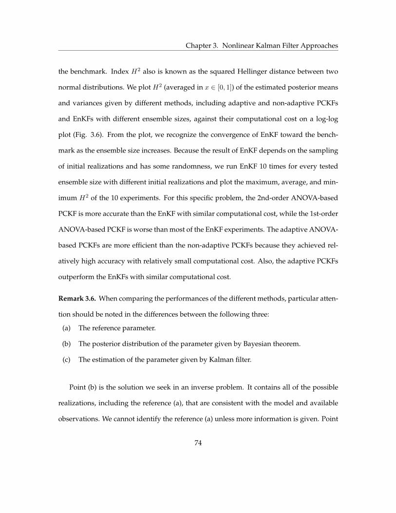
Chapter 3. Nonlinear Kalman Filter Approaches
the benchmark. Index H2 also is known as the squared Hellinger distance between two
normal distributions. We plot H2 (averaged in x ∈ [0, 1]) of the estimated posterior means
and variances given by different methods, including adaptive and non-adaptive PCKFs
and EnKFs with different ensemble sizes, against their computational cost on a log-log
plot (Fig. 3.6). From the plot, we recognize the convergence of EnKF toward the bench-
mark as the ensemble size increases. Because the result of EnKF depends on the sampling
of initial realizations and has some randomness, we run EnKF 10 times for every tested
ensemble size with different initial realizations and plot the maximum, average, and min-
imum H2 of the 10 experiments. For this specific problem, the 2nd-order ANOVA-based
PCKF is more accurate than the EnKF with similar computational cost, while the 1st-order
ANOVA-based PCKF is worse than most of the EnKF experiments. The adaptive ANOVA-
based PCKFs are more efficient than the non-adaptive PCKFs because they achieved rel-
atively high accuracy with relatively small computational cost. Also, the adaptive PCKFs
outperform the EnKFs with similar computational cost.
Remark 3.6. When comparing the performances of the different methods, particular atten-
tion should be noted in the differences between the following three:
(a) The reference parameter.
(b) The posterior distribution of the parameter given by Bayesian theorem.
(c) The estimation of the parameter given by Kalman filter.
Point (b) is the solution we seek in an inverse problem. It contains all of the possible
realizations, including the reference (a), that are consistent with the model and available
observations. We cannot identify the reference (a) unless more information is given. Point
74

Chapter 3. Nonlinear Kalman Filter Approaches
0 0.2 0.4 0.6 0.8 1 -4
-2
0
2
4
Adaptive PCKF criterion1 (average 64 simulations/loop)
0 0.2 0.4 0.6 0.8 1 -4
-2
0
2
4 EnKF 10000 realizations
0 0.2 0.4 0.6 0.8 1 -4
-2
0
2
4 EnKF 160 realizations
0 0.2 0.4 0.6 0.8 1 -4
-2
0
2
4 EnKF 40 realizations
0 0.2 0.4 0.6 0.8 1 -4
-2
0
2
4
PCKF based on 1st order ANOVA (21 simulations/loop)
0 0.2 0.4 0.6 0.8 1 -4
-2
0
2
4
Adaptive PCKF criterion2 (average 39 simulations/loop)
PCKF based on 2nd order ANOVA (201 simulations/loop)
0 0.2 0.4 0.6 0.8 1 -4
-2
0
2
4 EnKF 80 realizations
0 0.2 0.4 0.6 0.8 1 -4
-2
0
2
4
0 0.2 0.4 0.6 0.8 1 -4
-2
0
2
4
Adaptive PCKF criterion3 (average 38 simulations/loop)
x x x
x x x
x x x
Y
Y
Y
Y
Y
Y
Y
Y
Y
Figure 3.5: Comparison of the parameter estimations given by EnKFs, non-adaptivePCKFs and Adaptive PCKFs (Problem 1).
75

Chapter 3. Nonlinear Kalman Filter Approaches
10 1
10 2
10 -2
10 -1
10 0
Average number of model simulations per loop
H 2
EnKFs (max, average, min)
PCKF 1st order ANOVA
PCKF 2nd order ANOVA
Adaptive PCKF criterion1
Adaptive PCKF criterion2 Adaptive PCKF criterion3
Figure 3.6: Efficiency comparison between EnKFs, non-adaptive PCKFs and AdaptivePCKFs using H2 index (Case 1, Problem 1).
76

Chapter 3. Nonlinear Kalman Filter Approaches
(c) is an approximation to (b) that may be obtained with less computational cost (e.g., com-
pared with MCMC). The difference between (b) and (c) results from applying the Kalman
filter to a nonlinear model, and this error cannot be eliminated by enlarging either the en-
semble size in EnKF or the PCE terms in PCKF. Hence, rather than (a) or (b), we choose the
EnKF with large ensemble size as the benchmark.
Comparison Between Adaptive Criteria
To further study and compare the different adaptive criteria, we test our algorithm on Case
2 and Case 3. In Case 2, we set a smaller prior parameter variance. Because the parameter
varies in a smaller range, this makes input–output relation less nonlinear and results in
smaller 2nd-order ANOVA components. This case is designed to study how the adaptive
criteria respond to the change in the problem’s non-linearity. In Case 3, we assume the
observations are less accurate by setting larger observation errors. The purpose is to check
how the adaptive criteria react to the change in observation quality. Table 3.2 shows the
average number of PCE basis functions selected in the 10 loops by the three different cri-
teria. From Table 3.2, we see that Criterion 3 responds to the changes in Cases 2 and 3 by
retaining a smaller number of PCE basis functions compared with Case 1, which implies
that fewer 2nd-order components are computed in the ANOVA decomposition. Criterion
2 reduces the number of PCE basis functions for only Case 2 but is not sensitive to the
change in Case 3. Criterion 1 retains almost the same number of PCE basis functions in all
three cases. This result is consistent with our expectations. Criterion 1 selects 2nd-order
ANOVA components by distinguishing the important dimensions among all dimensions
77

Chapter 3. Nonlinear Kalman Filter Approaches
using 1st-order ANOVA, but it considers neither the nonlinearity of the problem nor the
quality of the observations. Criterion 2, which is an improvement upon Criterion 1, ex-
amines model nonlinearity. Finally, Criterion 3 improves Criterion 2 by considering the
quality of the observations.
To check the accuracies of the adaptive ANOVA-based PCKF using different criteria,
we once again solve the last two cases by different KF approaches and plot the index H2
of their results against the corresponding computational cost for Case 2 and Case 3 (Fig.
3.7 and Fig. 3.8, respectively). Apparently, the accuracies of the three adaptive ANOVA-
based PCKF methods are at almost the same level. Considering the computational cost,
we conclude that adaptive Criterion 3 offers the most effective selection of the PCE basis.
In fact, in the comparison with EnKFs, the 1st-order ANOVA-based PCKF performs much
better for Cases 2 and 3 than for Case 1. This also shows that a large number of 2nd-
order components are not necessary for the last two cases, and the response of reducing
PCE basis functions automatically made by Criterion 3 (also by Criterion 2 in Case 2) is
appropriate.
Table 3.2: Number of PCE basis functions selected by three criteria (average number of 10data assimilation loops).
Criterion 1 Criterion 2 Criterion 3
Case 1 64 39 38
Case 2 63 27 26
Case 3 69 38 26
78

Chapter 3. Nonlinear Kalman Filter Approaches
10 1
10 2
10 3
10 -4
10 -3
10 -2
10 -1
10 0
H 2
Average number of model simulations per loop
EnKFs (max, average, min)
PCKF 1st order ANOVA
PCKF 2nd order ANOVA
Adaptive PCKF criterion1
Adaptive PCKF criterion2 Adaptive PCKF criterion3
Figure 3.7: Efficiency comparison between EnKFs, non-adaptive PCKFs and AdaptivePCKFs using H2 index (Case 2, Problem 1).
79

Chapter 3. Nonlinear Kalman Filter Approaches
10 1
10 2
10 -3
10 -2
10 -1
EnKFs (max, average, min)
PCKF 1st order ANOVA
PCKF 2nd order ANOVA
Adaptive PCKF criterion1
Adaptive PCKF criterion2 Adaptive PCKF criterion3
Average number of model simulations per loop
H 2
Figure 3.8: Efficiency comparison between EnKFs, non-adaptive PCKFs and AdaptivePCKFs using H2 index (Case 3, Problem 1).
80

Chapter 3. Nonlinear Kalman Filter Approaches
3.3.2 Problem 2: Waterflooding of a Petroleum Reservoir
To further test and demonstrate the adaptive ANOVA-based PCKF, we apply it to a history
matching problem, which is commonly practiced in reservoir engineering. We calibrate a
petroleum reservoir model to the recorded well production data. Consider a synthetic,
two-dimensional, square-shaped reservoir bounded by no-flow boundaries (Fig. 3.9a).
The 1200-ft by 1200-ft domain is partitioned into 40 by 40 grid blocks, and the thickness of
every grid block is 30 ft. We simulate the physical process of two-phase flow (oil and water)
in the reservoir. Initially, the reservoir is saturated with 75% oil and 25% water (porosity
is 0.2). Four wells, two producers, and two water injectors are located at the four corners.
The oil is recovered from the reservoir using the waterflooding method: two injectors are
used to push oil toward the producers by injecting water, both at the constant rate of 300
stock tank barrels (STB) per day and the two production wells both produce fluids while
maintaining a constant bottom hole pressure (BHP) of 3000 psi. This production process is
simulated with the reservoir simulator ECLIPSE. In this process, the permeability k(x, y) of
the reservoir medium has significant influence on the fluid flow and determines how much
of the total oil stored in the reservoir may be recovered. However, due to the heterogeneity
of the permeability distribution and difficulty of precise measurement, we usually do not
have complete and accurate knowledge of k(x, y). In this example, k(x, y) is assumed to
be subject to a prior uncertainty. Y = log(k) is a stationary Gaussian random function, and
its prior mean and covariance are:
E(Y (x, y)) = µY , (3.51)
81

Chapter 3. Nonlinear Kalman Filter Approaches
Cov (Y (x1, y1) , Y (x2, y2)) = σ2Y exp
[
−(
x1 − x2ηx
)2
−(
y1 − y2ηy
)2]
, (3.52)
where the mean of log permeability is µY = 2 (this mean is calculated when permeability
is measured in the unit of millidarcy); variance σ2Y = 1; and the correlation factors in x and
y directions, ηx and ηy, are both 400 ft. A realization of Y is sampled from the prior distri-
bution and is assumed to be the true permeability field (Fig. 3.9b). Given the permeability
field, we can predict the water saturation in different stages during the waterflooding pro-
cess (Figs. 3.9c and 3.9d).
In this inverse problem, our objective is to estimate Y from the recorded production
data in different stages (also known as the production history). The available data include
the bottom hole pressure (BHP) recorded at the two injection wells, as well as the water
production rate (WPR) and the oil production rate (OPR) at the two production wells. The
data are generated from the true permeability field and are collected every 40 days at a
total of 15 time steps. The data observed at different time steps are assimilated sequen-
tially in Kalman filter loops. The errors associated with observations are assumed to be
independent normal with zero means and standard deviations being equal to 5% of the
observed values.
We solve this problem with adaptive ANOVA-based PCKF using Criterion 3. The PCE
representation for parameter Y is initialized using PCA with 20 random variables, which
results in a 20-dimensional inverse problem. Fig. 3.10 and Fig. 3.11 show the simulation
results with error bars of the well production history before and after data assimilations,
respectively. We observe that, due to the uncertain parameters, the simulation results in
82

Chapter 3. Nonlinear Kalman Filter Approaches
Inj2
Inj1
Pro1
Pro2 x
y
300
600
900
12
00
(ft
) 0
300 600 900 1200 (ft) 0
(a) A synthetic 2-d reservoir model.
40 300
600
900
12
00
(ft
) 0
300 600 900 1200 (ft) 0
(b) True log permeability field.
300
600
900
1200 (
ft)
0
300 600 900 1200 (ft) 0
(c) Water saturation at t=180 d.
0.25
0.3
0.35
0.4
0.45
0.5
0.55
0.6
0.65
0.7
300
600
900
12
00
(ft
) 0
300 600 900 1200 (ft) 0
(d) Water saturation at t=500 d.
Figure 3.9: Oil recovery from a reservoir by waterflooding.
83

Chapter 3. Nonlinear Kalman Filter Approaches
Fig. 3.10 do not match the observed production history and are subject to significant un-
certainties. After assimilating all of the observations, we note the simulations match the
production history well and the uncertainties are greatly reduced (Fig. 3.11). The esti-
mated mean and posterior standard deviation of the log permeability field Y (x, y) by the
adaptive ANOVA-based PCKF is plotted in Fig. 3.12. Compared with Fig. 3.9b, we see
that the estimated mean is not identical to the true permeability but captures the big trend,
i.e., high permeability in the upper right area and low permeability in the lower left area.
From Fig. 3.12b, it is apparent that the parametric uncertainty is reduced mainly in the
regions near the wells, especially the production wells (note that the prior standard devia-
tion is uniformly equal to 1). In the regions far away from the wells, the uncertainty is less
reduced, indicating the production data are less sensitive to the permeability at those lo-
cations. To accurately estimate the permeability of the entire domain, other measurements
would be necessary.
In Fig. 3.13, we plot the number of adaptively selected PCE basis functions in different
data assimilation loops. The most visible trend in this plot is that the adaptive criterion
increased the number of PCE basis functions from Day 180 until around Day 380. In fact,
this is the early period when the production wells started producing water, known as
“break- through.” During breakthrough, there are some radical changes in the production
history, such as a sudden increase in WPR and a decrease in OPR. Having more PCE terms
helps to accurately capture the model response during this period.
Finally, we compare the efficiency of the adaptive ANOVA-based PCKF with non-
adaptive PCKFs and EnKFs. Again, we use the EnKF with large ensemble size (2000) as
84

Chapter 3. Nonlinear Kalman Filter Approaches
0 100 200 300 400 500 600 0
100
200
300
400
100 200 300 400 500 600 0
0.5
1
1.5
2 x 10
4
0 100 200 300 400 500 600 -50
0
50
100
150
200
250
100 200 300 400 500 600 0
0.5
1
1.5
2 x 10
4
0 100 200 300 400 500 600 -50
0
50
100
150
200
250
0 100 200 300 400 500 600 0
100
200
300
400
Time (days) Time (days) Time (days)
Time (days) Time (days) Time (days)
BH
P o
f In
j1 (
psi
) B
HP
of
Inj2
(p
si)
WP
R o
f P
ro1
(S
TB
/D)
WP
R o
f P
ro2
(S
TB
/D)
OP
R o
f P
ro1
(S
TB
/D)
OP
R o
f P
ro2
(S
TB
/D)
Observation Simulated production history
(Mean+/-standard deviation)
Figure 3.10: Simulated production history with uncertainty quantification, before modelcalibration (Problem 2).
85

Chapter 3. Nonlinear Kalman Filter Approaches
Time (days) Time (days) Time (days)
Time (days) Time (days) Time (days)
BH
P o
f In
j1 (
psi
) B
HP
of
Inj2
(p
si)
WP
R o
f P
ro1
(S
TB
/D)
WP
R o
f P
ro2
(S
TB
/D)
OP
R o
f P
ro1
(S
TB
/D)
OP
R o
f P
ro2
(S
TB
/D)
100 200 300 400 500 600 0
0.5
1
1.5
2 x 10
4
100 200 300 400 500 600 0
0.5
1
1.5
2 x 10
4
100 200 300 400 500 600 -50
0
50
100
150
200
250
100 200 300 400 500 600 -50
0
50
100
150
200
250
100 200 300 400 500 600 0
100
200
300
400
100 200 300 400 500 600 0
100
200
300
400
Observation Simulated production history
(Mean+/-standard deviation)
Figure 3.11: Simulated production history with uncertainty quantification, after modelcalibration (Problem 2).
86
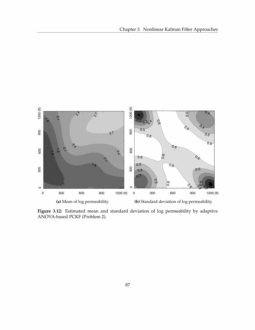
Chapter 3. Nonlinear Kalman Filter Approaches
1.8
2.1
2.1
2.4
1.5
3
0.9
300 600 900 1200 (ft) 0
30
0
60
0
90
0
12
00
(ft)
0
30
0
60
09
00
12
00
(ft)
(a) Mean of log permeability.
(ft)
30
0
60
0
90
0
12
00
(ft)
0
300 600 900 1200 (ft) 0
0.2
0.3
0.4
0.5
0.5
0.5
0.5
0.5
0.5
0.6
0.6
0.6
0.6
0.6
0.6
0.6
0.1
(b) Standard deviation of log permeability.
Figure 3.12: Estimated mean and standard deviation of log permeability by adaptiveANOVA-based PCKF (Problem 2).
87

Chapter 3. Nonlinear Kalman Filter Approaches
50 100 150 200 250 300 350 400 450 500 550 600 0
50
100
150
200
250
300
Time (Day)
Nu
mb
er
of
PC
E b
ase
s
Figure 3.13: Number of PCE bases adaptively selected by criterion 3 (problem 2).
88

Chapter 3. Nonlinear Kalman Filter Approaches
the benchmark and calculate the H2 indexes of the results given by different approaches
to measure their accuracy. Fig. 3.14 depicts the “accuracy versus computational cost”
chart. Notably, the non-adaptive PCKFs are almost at the same accuracy levels with the
EnKFs with comparable computational cost, but the adaptive ANOVA-based PCKF is able
to achieve higher accuracy with relatively low cost, making it the most efficient option
among all of the methods tested.
EnKFs (max, average, min)
PCKF 1st order ANOVA
PCKF 2nd order ANOVA
Adaptive PCKF criterion3
10 -2
10 -1
H 2
10 2
10 3
Average number of model simulations per loop
Figure 3.14: Efficiency comparison between EnKFs, non-adaptive PCKFs and AdaptivePCKFs using H2 index (problem 2).
89

Chapter 3. Nonlinear Kalman Filter Approaches
3.4 Discussions
In this chapter, we develope an adaptive ANOVA-based PCKF algorithm to solve non-
linear inverse modeling problems. Our research contributes to previous studies from the
following aspects, and these improvements make the adaptive ANOVA-based PCKF a
more flexible and efficient tool for inverse modeling problems when compared with clas-
sic PCKF.
(a) Our algorithm adaptively selects the PCE basis functions to represent uncertainties
for different models and in different Kalman filter loops of sequential data assimilation
problems, while, in classic PCKF methods, the PCE basis are pre-set by users and remain
fixed in all loops.
(b) We extend the adaptive functional ANOVA algorithm, which mainly is used in
solving forward uncertainty propagation problems, to solving inverse modeling problems.
(c) We propose two new criteria (Criteria 2 and 3 in Section 3.2.2) for adaptive func-
tional ANOVA decomposition, which are more efficient and especially suited for using
PCKF. Criterion 2 is not only able to detect the important input dimen- sions among all of
them, but it also compares the relative importance between the low- and high-order com-
ponents. Criterion 3 is a modified version of Criterion 2. It accounts for the quality of the
observations and is more effective for inverse modeling problems.
We have tested the developed method by solving the inverse problems for two flow in
porous media models. The new method has been demonstrated to be more efficient and
90

Chapter 3. Nonlinear Kalman Filter Approaches
reliable in comparison with non-adaptive PCKF and EnKF approaches.
Finally, there are two other points worth noting: 1) The major computational burden in
the new approach still is the model evaluations at collocation points. The extra computa-
tional cost caused by manipulating the PCE terms and judging the adaptive criteria does
not make a difference in the efficiency competition between the new and old Kalman filter
methods. 2) Even with adaptive basis selection, the PCKF approach is not supposed to
replace the EnKF for extremely high-dimensional problems, e.g., when the dimension is a
few hundred or higher. For these problems, the computational cost of the PCKF based only
on 1st-order ANOVA decomposition still may be comparable to or exceed that required by
EnKF.
91

Chapter 4
Adaptive Sampling via GP-based
Surrogates
In this chapter we study a more general inversion approach. In order to deal with nonlin-
ear models and non-Gaussian distributions, we abandon the assumptions of Kalman filter
and directly sample from the posterior distribution defined by Bayes’ theorem. Sampling
methods rely on a large number of model evaluations with different parameter points,
which is computationally costly and impractical for most inverse modeling problems. To
alleviate the computation burden we study the use of a GP-based surrogate to facilitate the
sampling process. Like any other surrogate models, the GP-based surrogate is an approx-
imation of the original model that can be evaluated with much less computation effort. In
addition, the GP-based surrogate gives an estimation of approximation error. This error
estimation is considered in the sampling algorithm to yield a more reliable estimation of
92
Chapter 4. Adaptive Sampling via GP-based Surrogates
posterior distribution of model parameters. Furthermore this estimation indicates where
to do local refinements if a more accurate surrogate is desired. We present a novel in-
version algorithm that consists of a series of adaptive sampling and surrogate refinement
loops, which captures the posterior accurately while keeping the computational cost as
low as possible. To further improve the sampling efficiency and better reproduce non-
Gaussian, especially multi-modal posteriors, we propose an importance sampler using
Gaussian mixture proposal distributions.
The structure of this chapter is as follows: first, we briefly discuss the sampling tech-
niques that are used in inverse modeling; we then review some necessary background
knowledge about GP-based surrogates before presenting the main algorithm, which will
be demonstrated with three examples; finally, we summarize the chapter with conclusions
and further discussions.
4.1 Sampling Methods
4.1.1 Markov Chain Monte Carlo
MCMC is able to sample from a posterior density of any form and in high dimensionality.
It forms a Markov chain which evolves in the parameter space under some rules. Those
rules make the chain equivalent to a sample from the objective density function. The classic
MCMC algorithm with Metropolis-Hastings sampling rule was developed by Metropolis
et al. (1953). A brief summary of the Metropolis-Hastings algorithm is described here.
93

Chapter 4. Adaptive Sampling via GP-based Surrogates
To sample from the posterior p(m|d∗), we start with an randomly selected initial point
m(0) and then build a Markov chain step by step. In the (j + 1)st step, a new point is
selected with the following rule:
1. A candidate point mq is generated from a proposal distribution q(·) which is easy to
sample from but may differ from our objective density p(m|d∗). q(·) could depend
on the point at previous step: q(·|m(j)).
2. The candidate point mq is accepted to be the (j +1)st point on the chain with proba-
bility γ, which depends on m(j) and mq through the following equation:
γ = min
(
1,p(mq|d∗)q(m(j)|mq)
p(m(j)|d∗)q(mq|m(j))
)
. (4.1)
If mq is rejected, the Markov chain stays at the previous point, m(j+1) = m(j).
The second step reshapes the sample from the proposal distribution q to the objective dis-
tribution. Note that: 1) for each proposed candidate point mq, one needs to call the sim-
ulator once to evaluate the model and compute the acceptance probability. This makes
MCMC a computationally expensive method; 2) the computation of γ does not require
to know h, the normalizing constant in the Bayesian theorem since it cancels in the ratio
expression.
94
Chapter 4. Adaptive Sampling via GP-based Surrogates
4.1.2 Importance Sampling
Similar to MCMC, importance sampling draws a sample from an arbitrary pdf in two
steps: proposal and correction. In the first step, a sample of points {m(1)q ,m
(2)q , ...,m
(nS)q }
is generated from a proposal distribution q(m), which may be different from the targeted
distribution but takes some simple form that is easy to sample from. In the second step, we
make this proposed sample reflect the distribution of p(m|d∗) by assigning each sample
point a weight
wj =p(m
(j)q |d∗)
q(m(j)q )
, j = 1, 2, ..., nS , (4.2)
The weight factors wj are then normalized such that their summation equals 1. Because of
this normalization, the normalizing constant h in the expression of posterior distribution
again does not have to be explicitly calculated. The calculation of the weights requires
model evaluations at each proposed points, which again makes the algorithm computa-
tional demanding. However, one advantage of importance sampling over MCMC is that
the model evaluations at different points may be run in parallel.
If a equal-weight sample is desired, we can draw a new sample among the points of
{m(1)q ,m
(2)q , ...,m
(nS)q } with probability of picking the point m
(j)q being wj . In our algo-
rithm, we use the method of systematic re-sampling (Arulampalam et al., 2002): generate
nS i.i.d. random numbers uj from the uniform distribution U(0, 1), and let m(j) = m(r)q ,
such that∑r
l=1wl ≥ uj and∑r−1
l=1 wl < uj . Finally, {m(1),m(2), ...,m(nS)} form an equal-
weight sample representing the objective posterior distribution.
Importance sampling also may be used for sequential data assimilation problems, which
95

Chapter 4. Adaptive Sampling via GP-based Surrogates
leads to the algorithm of sequential importance sampling, also known as particle filter
(Gordon et al., 1993). In particle filter, the weight associated with each point is updated
whenever new data become available so that the new information is assimilated.
4.1.3 Simulated Annealing
In most inverse modeling problems, the regions in the parameter space with non-negligible
posterior distribution only covers a tiny portion of that of the prior, which results in spiky
and rugged posterior pdf. As a result, in a MCMC implementation, most of the proposed
points do not hit the posterior and hence are rejected, whereas in importance sampling,
most of the proposed points would end up with nearly-zero weights. For such problems,
an extremely long chain or an extremely large sample size is necessary to achieve a reliable
representation of the posterior distribution. To alleviate the difficulty, one may sample
from a pdf that is modified from the original posterior distribution
pτ (m|d∗) = h · exp[
ln p(m|d∗)
τ
]
, (4.3)
where τ ≥ 1 is a parameter called temperature. When τ = 1, the modified pdf (4.3) is
equivalent to the original posterior pdf. When a larger temperature is used, the pdf (4.3)
becomes a flattened version of the original posterior and hence easier to sample from. See
Fig. 4.1 for an example. In practice, one can start with a high temperature, which is then
gradually decreased to approach the real posterior.
96

Chapter 4. Adaptive Sampling via GP-based Surrogates
−2 −1 0 1 20
10
20
30
40
50
60
70
80
m
pτ
τ = 1
−2 −1 0 1 20
5
10
15
20
25
30
m
pτ
τ = 8
−2 −1 0 1 20
2
4
6
8
10
m
pτ
τ = 64
−2 −1 0 1 20
0.5
1
1.5
2
2.5
3
3.5
m
pτ
τ = 512
Figure 4.1: An example of a pdf at different temperatures.
97

Chapter 4. Adaptive Sampling via GP-based Surrogates
4.2 Gaussian Process-based Surrogates
4.2.1 Basic Idea
In this section, we give a review of Gaussian process-based surrogates and demonstrate
how they can be used to facilitate the Bayesian inversion. For simplicity, we first consider
models with only one output variable, and then extend the methodology to general models
with multidimensional output.
The methods of using Gaussian processes to approximate deterministic computer model
outputs were previously developed in different studies (Sacks et al., 1989; Currin et al.,
1991; Kennedy and O’Hagan, 2001). Though formulated by different researchers and from
different perspectives, these methods share the same fundamental philosophy. Essen-
tially, the true model response g(m) is assumed to be a realization of a stochastic process
G(m). For mathematical convenience, this stochastic process is often chosen to be a Gaus-
sian/normal process:
G(m) ∼ N (µ(·), C (·, ·)) , (4.4)
which is characterized by its mean function µ(·) and covariance function C (·, ·) (see next
subsection for detailed discussion about the covariance function). Eq. (4.4) means that the
model response at n different parameter points {m(1),m(2), ...,m(n)} follow a multivariate
Gaussian distribution N(µ,C), where the mean vector and covariance matrix are µi =
µ(m(i)), Cij = C(m(i),m(j)), i, j = 1, ...n. Specifically, at any parameter point m, the
model response is expressed as a Gaussian random variable.
98

Chapter 4. Adaptive Sampling via GP-based Surrogates
The uncertainty associated with the model output is caused by the fact that we are not
able to actually evaluate the original model at that parameter point due to the computa-
tional cost, but can only give an approximate estimation. To reduce this uncertainty, we
may condition this process (Eq.4.4) to model evaluations at nB parameter points, which
we call the base points: B = {m(1)B ,m
(2)B , ...,m
(nB)B }. The conditional process, G|B(m), is
still a a Gaussian process, and its mean and variance at a parameter point m are given by
µ|B(m) = µ(m) + CmBC−1BB (g(B)− µ(B)) , (4.5)
and
σ2|B(m) = C(m,m)− CmBC−1BBCBm, (4.6)
respectively. µ(·) and C (·, ·) are the mean and covariance functions defined in the uncon-
ditional process (4.4). CmB is a 1 by nB vector where the ith element is C(m,m(i)B ). CBB is
a nB by nB matrix where the element on the ith row and the jth column is C(m(i)B ,m
(j)B ).
g(B) and µ(B) are both nB by 1 vectors. While the former contains the evaluated model
output at the nB base points, the latter includes the unconditional mean defined on the
same points. Note that the conditioned variance (Eq.4.6) at the base points becomes zero,
which shows our knowledge of the exact model output at these points. Moreover, the un-
certainty at any other point m is also reduced because of the information gained through
the correlations between m and the base points.
The conditional distribution provides a surrogate to the original model: g(m) = g(m)+
eg, where g(m) = µ|B(m) can be used as an approximation of the true model response,
99

Chapter 4. Adaptive Sampling via GP-based Surrogates
and eg is the estimated surrogate error which follows the normal distribution N(
0, σ2|B
)
.
The likelihood function may be derived from this surrogate. Consider an example of case
4 discussed in Chapter 2. Suppose the observation of the model output has an error of
eo ∼ N(0, σ2o) independent of the surrogate error, then the total error, e = eg + eo, is also a
Gaussian random variable with the distribution of N(0, σ2|B + σ2o). The likelihood function
takes the form of fe(d∗ − g(m)), where fe(·) is the pdf of e.
To illustrate the GP surrogate-based Bayesian inversion, we consider a simple nonlin-
ear model with only one input parameter and one output variable: d = g(m). The model
parameter is subject to a prior uncertainty: m ∼ N(0, 0.52). To estimate the parameter,
an observation of the model output is made: d∗ = 1.1, which is also associated with an
observation error: eo ∼ N(0, 0.022). When the model is expensive to evaluate, we cannot
afford to compute the exact model response at every points, but we assume it resembles a
realization of a Gaussian process described by Eq.(4.4) with a constant mean µ(m) = 1.5
for any m and a covariance function C(m(1),m(2)) = 4 exp(
−0.75(m(1) −m(2))2)
. Note
that according to this assumption, the model output at any parameter point m is a Gaus-
sian random variable with standard deviation of 2. To reduce this uncertainty, we evaluate
the model d = g(m) at three base points B = {m(1)B = −
√3/2,m
(2)B = 0,m
(3)B =
√3/2},
and condition the Gaussian process to these base points. This conditional process as a
surrogate to the original model is plotted in Fig. 4.2. We see that the conditional mean
approximates the true model response, whereas the conditional standard deviation shows
the estimated approximation error. The surrogate is accurate at the points where original
model is evaluated while some surrogate uncertainty remains at other parameter points.
100

Chapter 4. Adaptive Sampling via GP-based Surrogates
Nonetheless, the overall uncertainty is greatly reduced after the conditioning. We also plot
in Fig.4.2 two posterior distributions of m, one derived from the GP-based surrogate and
the other from the true model response. The latter one is the true solution of this Bayesian
inverse problem, however, it requires the evaluation of model g(m) at a large number of
parameter points. Two spikes are seen in this distribution, showing two distinct parameter
values that may result in the observed output value. Also, the right spike is taller than the
left one, which is because the prior distribution puts more weight on the right solution.
The posterior pdf derived from the surrogate also accurately captures the left solution. But
the exact location of the right solution is not identified because the surrogate is subject to
a relatively large error in that region. Instead, we observe that the posterior pdf outlines
a larger region where the right solution might exist. This observation motivates us to add
one refinement base point (m = 0.4) in that region to improve the local accuracy. The re-
fined surrogate and the corresponding posterior distribution are shown in Fig. 4.3. With
one more refinement point (and a total of four base points and four model evaluations), the
GP-based surrogate is accurate enough around both solutions, and the resulting posterior
pdf is in a good agreement with the one obtained from the true model response. Finally,
Fig. 4.4 demonstrates the posterior computed from the surrogate without considering the
surrogate error. Assuming the surrogate is accurate enough, we simply substitute the orig-
inal model g(·) with the mean response of the GP g(·) when calculating the likelihood (2.4).
However, we see that the estimated right spike is biased due to the inaccurate approxima-
tion of the surrogate, and the true solution is mistakenly excluded from the posterior. The
posterior estimation of the right solution is precise (small reported uncertainty) but wrong.
Moreover, without an estimation of the surrogate, we have no clue of whether refinement
101

Chapter 4. Adaptive Sampling via GP-based Surrogates
points are needed.
-1.5 -1 -0.5 0 0.5 1 1.5 -1
0
1
2
3
4
m
g(m)
-1.5 -1 -0.5 0 0.5 1 1.5 0
10
20
30
40
50
60
m
p(m|d*)
Result by true model response
Result by surrogate response
True model response
Observa5on
Response of GP-‐based surrogate (mean+/-‐sd)
Model evalua5ons at base points
Figure 4.2: Comparison between the true and GP-based surrogate model responses, andtheir corresponding posterior distributions of the model parameter given an observationof the model output. The surrogate and its error estimation are represented by a Gaussianprocess conditioned to model evaluations at three base points.
102
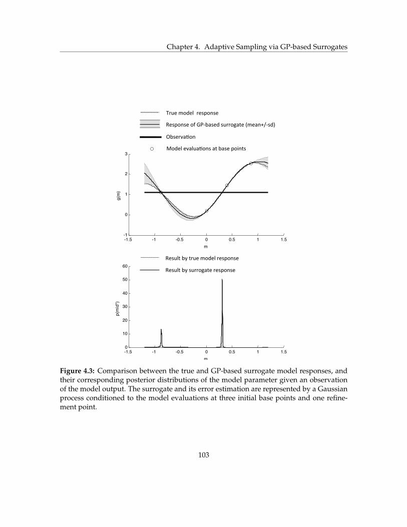
Chapter 4. Adaptive Sampling via GP-based Surrogates
-1.5 -1 -0.5 0 0.5 1 1.5 -1
0
1
2
3
m
g(m)
-1.5 -1 -0.5 0 0.5 1 1.5 0
10
20
30
40
50
60
m
p(m|d*)
Result by true model response
Result by surrogate response
True model response
Observa5on
Response of GP-‐based surrogate (mean+/-‐sd)
Model evalua5ons at base points
Figure 4.3: Comparison between the true and GP-based surrogate model responses, andtheir corresponding posterior distributions of the model parameter given an observationof the model output. The surrogate and its error estimation are represented by a Gaussianprocess conditioned to the model evaluations at three initial base points and one refine-ment point.
103

Chapter 4. Adaptive Sampling via GP-based Surrogates
-1.5 -1 -0.5 0 0.5 1 1.5 -1
0
1
2
3
4
m
g(m
)
m
-1.5 -1 -0.5 0 0.5 1 1.5 0
10
20
30
40
50
60
p(m
|d*)
Result by true model response
Result by surrogate response
True model response
Observation
Mean response of GP-based surrogate
Model evaluations at base points
Figure 4.4: Comparison between the true and mean response of the surrogate model, andtheir corresponding posterior distributions of the model parameter given an observationof the model output. The surrogate is built by a Gaussian process conditioned to modelevaluations at three base points. The surrogate error is not considered when computingthe posterior distribution.
104

Chapter 4. Adaptive Sampling via GP-based Surrogates
4.2.2 Selection of Mean and Covariance functions
The properties of a Gaussian process’ realizations are determined by the mean and co-
variance functions in Eq.(4.4). So the quality of a GP-based surrogate is dependent on
the proper selection of these functions according to our prior knowledge about the prop-
erties of the model response. The mean function depicts the major trend of the model
response. For instance, we can choose from the simplest forms such as a constant function
µ(m) = µ0 if we know little about the model response, or more complicate forms such as
a linear regression function µ(m) = µ0 + βTm, where β is the coefficients vector. A group
of commonly used covariance functions for a model with nm input parameters take the
following form
C(m(1),m(2)) = σ2 exp
[
−nm∑
i=1
|m(1)i −m
(2)i |αi
ηi
]
. (4.7)
Eq.(4.7) assumes that the covariance between g(m(1)) and g(m(2)) depends on the distance
separating the two points m(1) and m(2). The shorter the distance is, the stronger the
correlation is, and a perfect positive correlation is achieved as the distance approaches 0.
Such a covariance function is used when we believe the model response is a continuous
function. Furthermore the distances along different input dimensions may have different
impacts on the correlation, which is controlled by the correlation length parameters ηi and
the power parameters αi. ηi, which is a positive real number, determines the typical cor-
relation length along the ith input dimension, i.e., the distance beyond which two points
have relatively weak correlation. On the other hand, αi, which could be a real number
between 1 and 2, controls the smoothness of the realizations. Fig.4.5 shows four GP-based
surrogates built on the same three interpolation points but from different covariance func-
105

Chapter 4. Adaptive Sampling via GP-based Surrogates
tions of the unconditional process. In the first three cases, power parameter α is equal to 2
(known as the Gaussian type correlation function). By comparison among the three poste-
rior processes we see the effect of the correlation length factor η. Large η imposes a strong
correlation constraint and tends to underestimate the surrogate error (Fig.4.5c), whereas
short η results in an overestimated surrogate error (Fig.4.5b). Only a proper correlation
length leads to a good approximation of the true model response (Fig.4.5a). In the fourth
case, we change parameter α to 1 (known as the exponential type correlation function). We
see that the mean response in this case is less smooth (not differentiable at the interpolation
points) comparing with the results of the Gaussian correlation function.
In practice, the mean and covariance functions, or the parameters that determine these
functions (e.g. µ0,β, σ2, ηi, αi) could be estimated also from the model evaluations at the
base points. For example, we can choose the maximum likelihood estimator (MLE) of the
parameters, i.e., the values of the parameters that maximize the joint pdf of the model
responses at the nB base points, which is multi-variate Gaussian N (µ(B), C(B,B)).
To further check the quality of the GP-based surrogate, one could implement a cross
validation procedure, which does not incur any extra model evaluations. That procedure
is to leave one base point out of the conditioning step and see whether the resulting Gaus-
sian process can predict the true model output at this point. Repeat this process for every
base point. Failing in cross validation signals that the surrogate is not reliable. For ex-
ample, if the predicted mean response deviates from the true model response by as far
as three standard deviations of the estimated approximation error, we reject the surrogate
and build a new one with some other mean and covariance functions.
106

Chapter 4. Adaptive Sampling via GP-based Surrogates
-1 -0.5 0 0.5 1 -1
0
1
2
3
4
5
m
g(m
)
-1 -0.5 0 0.5 1 -1
0
1
2
3
4
5
m
g(m
)
-1 -0.5 0 0.5 1 -1
0
1
2
3
4
5
m
g(m
)
-1 -0.5 0 0.5 1 -1
0
1
2
3
4
5
m
g(m
)
(1) (2) 2(1) (2) | |
( , ) 4exp[ ]3
m mC m m
(a)
(c)
(b)
(d)
Estimated response
(Mean+/-standard deviation) True model response Interpolation points
(1) (2) 2(1) (2) | |
( , ) 4exp[ ]4 / 3
m mC m m
(1) (2) 2(1) (2) | |
( , ) 4exp[ ]1/ 3
m mC m m
(1) (2)(1) (2) | |
( , ) 4exp[ ]4
m mC m m
Figure 4.5: Four GP-based surrogates built on the same base points but with differentassumptions of the covariance function.
107

Chapter 4. Adaptive Sampling via GP-based Surrogates
4.2.3 Models with Multiple Output Variables
So far we have been discussing the GP-based surrogate for scalar functions. A simple ap-
proach to extend this method to models with multiple output variables is to build different
GP surrogates for each of them. However, in many subsurface flow models, the outputs
are usually temporal and spatial functions and thus high-dimensional, which makes the
construction of GP-based surrogates difficult and expensive. But on the other hand, these
output variables are often correlated, so we can represent the high-dimensional output
with its low-dimensional principal components (Higdon et al., 2008).
d = d0 +Dρ, (4.8)
where d0 is the mean of the output vector d, D is a matrix whose columns are the principal
components of the output vector, and ρ = [ρ1, ρ2, ..., ρnP ]T is a vector of the corresponding
coefficients of each principal components. With this representation we can approximate
each element of vector ρ with GP-based surrogates instead of approximating vector d. Not
only ρ usually contains much less elements than d, ρi are also decorrelated, which makes
the mathematical manipulation easier. At any parameter point m, the model output d(m)
is expressed as a multi-variate random vector, with mean
µd(m) = d0 +Dµρ(m) (4.9)
and covariance
Cdd(m) = DCρρ(m)DT , (4.10)
108

Chapter 4. Adaptive Sampling via GP-based Surrogates
where µρ(m) and Cρρ(m) are the mean vector and covariance matrix of ρ(m) provided by
the GP-based surrogates. Similar to the single-output situation, we can write the surrogate
model for d as d(m) = g(m) + eg(m), where g(m) = µd(m) provides an approximation
of the original model response and eg ∼ N (0,Cdd) reflects the estimation of the approx-
imation error. Substituting this surrogate and its error estimation into Eq.(2.5) or Eq.(2.6)
yields the likelihood function for Bayesian inversion.
Moreover, instead of dealing with the original values of the output variables, we nor-
malize each output variable using its corresponding observation error: di = di/σei . This
procedure puts more weights on those output variables with more accurate observation.
4.3 Adaptive Re-sampling and Refinement Algorithm
Sampling from the posterior, even with the help of a surrogate model, is not a trivial task,
especially when the posterior is multi-modal and/or covers only a tiny fraction of the prior
distribution. In this section, we present an algorithm that adaptively refines the GP-based
surrogate and samples from the targeted posterior distribution. The algorithm starts with
an initial surrogate and an initial sample of parameter points, and then goes through a
series of loops, each consists of a re-sampling step and a refinement step. The re-sampling
and refinement steps are implemented alternatively with the assistance of each other and
gradually achieve a sample of points that accurately show the targeted posterior.
109

Chapter 4. Adaptive Sampling via GP-based Surrogates
4.3.1 Initialization
We start by building a GP-based surrogate on nB initial base points,B0 = {m(1)B , ...,m
(nB)B },
selected according to the prior distribution. In our algorithm the initial base points are gen-
erated using the method of latin hyper-cube sampling, which results in a relatively good
coverage of the entire prior distribution (McKay et al., 1979). nB , the number of initial base
points and the number of model evaluations needed in this step does not have to be very
large because we do not require the surrogate to be globally accurate. The initial surrogate
will be adaptively refined in the following steps. Also, we generate an initial sample of pa-
rameter points S0 = {m(1)S0,m
(2)S0, ...,m
(nS)S0
} from the prior distribution. which will shrink
to the posterior distribution in the following refinement and re-sampling loops. Note that
we could afford to have a much larger number of sample points nS than the base points
since the sampling and re-sampling procedures do not incur simulations of the original
model when a surrogate is used instead. After the initialization, we proceed to a series of
re-sampling and surrogate refinement loops.
4.3.2 Re-sampling via GP-based Surrogate
In each new loop, say the ith loop, a new sample of points are generated from p(m|d∗, Bi−1) =
h· p(d∗|m, Bi−1)p(m), which is the posterior distribution defined through the surrogate
built upon base points Bi−1 in previous loop. In our algorithm, we choose the method of
importance sampling to carry out this step (see section 4.1.2). One of the most challenging
parts in importance sampling is the selection of the proposal distribution q(m). Although,
110

Chapter 4. Adaptive Sampling via GP-based Surrogates
theoretically, any distribution that covers the domain where the targeted distribution exists
may be used as the proposal distribution, a properly selected q(m) could greatly improve
the qualify of the sample. An ideal proposal distribution should be as close to the targeted
distribution as possible. However, in the context of Bayesian inversion, we have no idea
of where to construct such a proposal distribution since the target itself, i.e., the posterior,
is unknown. Usually, the proposal distribution is chosen as the prior p(m). Note that in
most problems the prior has a simple pdf such as uniform or Gaussian, which is easy to
sample from. But often the posterior distribution concentrates only on a small portion of
the regions covered by the prior distribution. As a result, most of the proposed sample
points except a few do not hit the posterior and end up with nearly-zero weights, which
causes a large sampling error. This phenomenon is known as “sample degeneracy”.
Our algorithm brings a remedy to this issue by using a different proposal distribu-
tion that is much closer to the target. Note that the posterior distribution we seek in
current loop, p(m|d∗, Bi−1), is not completely unknown because it is an improvement of
the posterior we estimated in previous loop, which we have a sample of points Si−1 =
{m(1)Si−1
,m(2)Si−1
, ...,m(nS)Si−1
} showing its distribution. Inspired by this observation, we choose
a proposal qi(m) in the ith loop such that the points in Si−1 are closely incorporated. For
the specific form of qi(m), we use a Gaussian mixture model, which is not only easy to
draw sample from, but also flexible enough to fit different distributions of Si−1, includ-
ing multi-modal distributions induced by strongly nonlinear model g(·). To fit the sample
Si−1 into a Gaussian mixture model, we first divide the nS sample points into nc groups,
or clusters, with a clustering method such as K-means (Hartigan and Wong, 1979). Each
111

Chapter 4. Adaptive Sampling via GP-based Surrogates
cluster of points approximately represents a nm-dimensional multivariate Gaussian pdf
fN(
m;µ(j),C(j))
, j = 1, 2, ...nc, where the mean µ(j) and covariance C(j) are estimated
from the jth cluster of points. A Gaussian mixture distribution as the proposal is then
constructed
qi(m) =
nc∑
j=1
n(j)S
nSfN
(
m;µ(j),C(j))
, (4.11)
where n(j)S is the number of points in the jth cluster. A sample point from this pdf can
be obtained simply in two steps: 1) randomly picking a cluster j with probability n(j)S /nS ;
and 2) generating a sample point from the Gaussian distribution fN(
m;µ(j),C(j))
. Fig.
4.6 shows an example of fitting a sample of points into a Gaussian mixture distribution
and a new sample regenerated from it.
4.3.3 Refinement of Surrogate Models
After obtaining the new sample in the ith new loop, we check whether further refinement
of the surrogate is needed. If so, we refine the surrogate by adding one more base point
m(n+i)B to the existing ones to form a new set of base points Bi. The selection of the new
base point follows two criteria which ensure the efficiency of the refinement scheme. First,
the refinement point should be within or close to the regions of posterior distribution; sec-
ond, the refinement point should not be placed at a location where the surrogate is already
accurate enough. Note that the sample points obtained from the previous loop provide
an approximate representation of the posterior distribution (though they usually cover a
larger region than the true posterior because of the consideration of surrogate error), which
112

Chapter 4. Adaptive Sampling via GP-based Surrogates
−6 −4 −2 0 2 4 6−4
−3
−2
−1
0
1
2
3
4
m1
m2
(a)
−6 −4 −2 0 2 4 6−4
−3
−2
−1
0
1
2
3
4
m1
m2
cluster 1
cluster 2
cluster 3
cluster 4
(b)
0.01
0.010.01
0.01
0.0
1
0.01
0.01
0.01
0.0
1
0.02
0.02
0.02
0.0
2
0.0
2
0.02
0.02
0.02
0.0
2
0.0
3
0.0
3
0.03
0.0
3
0.0
3
0.03
0.03
0.030.0
4
0.04
0.04
0.0
4
0.0
40.0
4
0.04
0.04
0.05
0.05
0.0
50.0
5
0.05
0.05
0.05
0.06
0.0
6
0.06 0.06
0.070.07
0.07
m1
m2
−6 −4 −2 0 2 4 6−4
−3
−2
−1
0
1
2
3
4
(c)
−6 −4 −2 0 2 4 6−4
−3
−2
−1
0
1
2
3
4
m1
m2
(d)
Figure 4.6: Use a Gaussian mixture distribution as the proposal distribution for importancesampling: an illustrative example. (a) 300 original sample points; (b) clustering of theoriginal sample points; (c) Gaussian mixture distribution fitted from the clusters; (d) 1000new sample points proposed from the Gaussian mixture distribution.
113

Chapter 4. Adaptive Sampling via GP-based Surrogates
makes them candidate points meeting the first criterion. So we choose the refinement point
to be the point with the largest surrogate error among all the sample points from the pre-
vious loop. However, if the surrogate is accurate enough at all candidate points, we stop
the refinement loops and report the current sample points as the sample that represent the
targeted posterior distribution.
Note that this algorithm can be easily modified to add multiple refinement base points
in each loop, which is particularly useful when the simulations with different parameter
points can be run in parallel.
4.3.4 Summary of Work Flow
The implementation procedures of the adaptive sample-refine algorithm are summarized
here:
1. Input to the algorithm:
• original model, g(·);
• prior distribution of model parameters, p(m);
• observation of model output, d∗, and associated observation errors;
• number of initial base points, nB ;
• maximum number of base points, also the maximum number of evaluations of
the original model, nB ;
• number of sample points used to represent the posterior distribution, nS ;
114

Chapter 4. Adaptive Sampling via GP-based Surrogates
• surrogate error threshold, e
2. Initialization:
• generate nB initial base points B0 = {m(1)B ,m
(2)B , ...,m
(nB)B } according to p(m)
using latin hyper-cube sampling;
• compute the output values of the original model at the base points: d(j) =
g(
m(j)B
)
, j = 1, 2, ..., nB ;
• construct a GP-based surrogate of the original model conditioned to the base
points: G(m|B0);
• draw nS initial sample points S0 = {m(1)S0,m
(2)S0, ...,m
(nS)S0
} according to the prior
distribution p(m).
3. Re-sampling via surrogate in the ith loop
• group the sample points Si−1 into clusters with K-means method;
• construct a proposal distribution qi(m) using a Gaussian mixture model (Eq.4.11);
• generate nS proposed sample points {m(1)q ,m
(2)q , ...,m
(nS)q } from qi(m), and
compute their corresponding weights {w1, w2, ..., wnS} using Eq.(4.2) via the
surrogate model G(m|Bi−1);
• draw a equal-weight sample Si = {m(1)Si,m
(2)Si, ...,m
(nS)Si
} from the weighted pro-
posed sample using systematic re-sampling method.
4. Refine surrogate in the ith loop
• check the approximation error of the GP-based surrogate response by calcu-
lating its standard deviation σ|B(m) using Eq.(4.6) at each sample point of Si,
115

Chapter 4. Adaptive Sampling via GP-based Surrogates
locate the point m∗ where the surrogate response has the largest standard devi-
ation;
• if the surrogate error is small enough: σ|B(m∗) < e, or the maximum number of
model evaluation is reached: nB + i > nB , stop, and report the sample Si as the
final solution of the inverse problem;
• if the stop criterion is not met, let m∗ be the refinement point m(n+i)B , add it to
current base points, and update the GP-based surrogate use the new set of base
points;
• proceed to step 3: Re-sampling via surrogate of the next loop.
4.4 Illustrative Examples
4.4.1 Problem 3: Test on an Algebraic Function
To better visualize the surrogate and the adaptive refinement process, we first apply our
algorithm to an algebraic model with only 2 input parameters and 1 output variable:
d = g(m1,m2) = m1m2. The prior distributions of m1 and m2 are both uniform on [-1,1]
and are independent with each other. We have an observation of model output d∗ = 0.4,
which is subject to a normally distributed observation error, eo ∼ N(0, 0.012). The objec-
tive is to estimate the model parameters from this observation and quantify the remaining
uncertainty. Moreover, we assume the analytic expression of g(·) is not known and it can
only be evaluated for specific input values, just like a simulator we would encounter in
116

Chapter 4. Adaptive Sampling via GP-based Surrogates
most inverse problems. We seek a sample of points representing the posterior distribution
defined by the Bayes’ rule. Even though this model has a simple form, its strong non-
linearity results in a spiky and bi-modal posterior, which is extremely difficult to sample
from using a classic sampling method.
To start our algorithm, we set the number of initial base points nB = 9, the number
of sample points nS = 2000, and the surrogate threshold e = 0.01, which is equal to
the standard deviation of the observation error. The initial surrogate response and the
estimation of the approximation error, which are represented by the mean and the standard
deviation of the GP-based surrogate, respectively, are shown in Fig. 4.7. We see that the
approximation error is pinned down to zero at the base points, but remains relatively large
(comparing with the threshold) in some other regions.
Contour lines Base points
Mean Standard deviation
m1 m1
m2
m2
-1 -0.5 0 0.5 1 -1
-0.5
0
0.5
1
-1 -0.5 0 0.5 1 -1
-0.5
0
0.5
1
Figure 4.7: Mean and standard deviation of the GP-based surrogate built on 9 initial basepoints (Problem 3).
117

Chapter 4. Adaptive Sampling via GP-based Surrogates
The further adaptive refinement process is illustrated in Fig.4.8 and Fig.4.9. We see that
in each refinement loop, a sample of points are generated via the surrogate (Fig.4.8). Ini-
tially, the sample points are loosely spread around the upper right and lower left corners,
which roughly outline the regions of the true posterior but do not provide an accurate
representation. In each loop, a new base point is selected among the sample points and
is used to improve the local accuracy of the surrogate (Fig.4.9). The stop criterion is met
after 6 refinements. Even though the surrogate is still not globally accurate, we see that the
adaptive refinement scheme ensures the surrogate accuracy in the regions around the tar-
geted posterior distribution, and as a result, a nice sample of the posterior is obtained. The
final sample representing the posterior is achieved at the cost of only 15 model evaluations,
including 9 for building the initial surrogate and 6 for adaptive refinement.
118

Chapter 4. Adaptive Sampling via GP-based Surrogates
-1 -0.5 0 0.5 1-1
-0.5
0
0.5
1
m1
m2
-1 -0.5 0 0.5 1-1
-0.5
0
0.5
1
m1
m2
-1 -0.5 0 0.5 1-1
-0.5
0
0.5
1
m1
m2
-1 -0.5 0 0.5 1-1
-0.5
0
0.5
1
m1
m2
-1 -0.5 0 0.5 1-1
-0.5
0
0.5
1
m1
m2
-1 -0.5 0 0.5 1-1
-0.5
0
0.5
1
m1
m2
Sample points Existing base points Newly added base point
(loop 1)
(loop 3)
(loop 5)
(loop 2)
(loop 4)
(loop 6)
Figure 4.8: Sample points obtained in different re-sampling and refinement loops (Problem3).
119

Chapter 4. Adaptive Sampling via GP-based Surrogates
-1 -0.5 0 0.5 1-1
-0.5
0
0.5
1
m1
m2
-1 -0.5 0 0.5 1-1
-0.5
0
0.5
1
m1
m2
-1 -0.5 0 0.5 1-1
-0.5
0
0.5
1
m1
m2
-1 -0.5 0 0.5 1-1
-0.5
0
0.5
1
m1
m2
-1 -0.5 0 0.5 1-1
-0.5
0
0.5
1
m1
m2
-1 -0.5 0 0.5 1-1
-0.5
0
0.5
1
m1
m2
Existing base points Newly added base point
(loop 1)
(loop 3)
(loop 5)
(loop 2)
(loop 4)
(loop 6)
Figure 4.9: Standard deviations of the surrogate errors in different refinement loops (Prob-lem 3).
120

Chapter 4. Adaptive Sampling via GP-based Surrogates
4.4.2 Problem 4: I-C Fault Model
In the second example, we applied our algorithm to the history matching problem of a
reservoir model known as I-C Fault model (Tavassoli et al., 2004; Carter et al., 2006). The
model is designed such that the dependent relationship between the production history
and the uncertain model parameters is strongly nonlinear, which results in a complex
multi-modal posterior. In the original study of (Tavassoli et al., 2004), the authors thor-
oughly explored the three-dimensional parameter space with the simulations of 159,645
randomly generated realizations. But, the realization that best matched the production
history did not reflect the true geological properties of the reservoir and yielded a wrong
prediction of future production. In a following research paper, Christie et al. (2006) studied
the quantification of the posterior uncertainty by sampling from the posterior distribution.
Machine learning algorithms including Genetic Algorithms and Artificial Neural Network
were used to reduce the computational burden. However, thousands of model simulations
were still needed to achieve a satisfying sample.
We give a brief review of the I-C Fault model, while more details may be found in
the above cited references. The I-C Fault model represents the 2-D vertical cross section
of an oil reservoir that consists of six layers of alternating high- and low-permeable sand
(Fig.4.10). The reservoir is 1000 ft wide and 60 ft thick, where the thickness of the six layers
is an arithmetic progression from the bottom (7.5 ft) to the top (12.5ft). The reservoir is
divided into two parts by a fault in the middle. A water injection well and a production
well are located at the left and right boundaries, respectively, both operating at constant
pressures. The upper and lower boundaries are bounded by no flow boundary conditions.
121

Chapter 4. Adaptive Sampling via GP-based Surrogates
Figure 4.10: I-C Fault model (Carter et al., 2006), distances are measured in feet (Problem4).
The model has three uncertain input parameters with independent and uniform prior
distributions: the fault throw (h ∈ [0, 60]ft), the permeability of the good-quality sand
(kg ∈ [100, 200]md), and the permeability of the poor-quality sand (kp ∈ [0, 50]md). For
each realization sampled from the parameter space, the corresponding production history
(water cut and oil production rate in this problem) could be simulated from the model.
Fig.4.11 shows the simulation results from an ensemble of input realizations drawn from
the prior distribution. It is seen that the variations of the input parameters cause a large
uncertainty in the simulation results. To reduce the uncertainty, we calibrate the input pa-
rameters to the observations of the ”synthetic true” production history, which are recorded
every month in the first three years of production. The observed data are generated
from the simulation based on a reference parameter point (h0 = 10.4ft, kg0 = 131.6md,
122

Chapter 4. Adaptive Sampling via GP-based Surrogates
kp0 = 1.3md), and are perturbed randomly according to the observation errors, which we
assume are normally distributed, with zero means and standard deviations equal to 5% of
the predicted standard deviations (prior uncertainty) of the simulation results.
time (days)
Oil
Pro
duction R
ate
(S
TB
/day)
time (days)
Wate
r C
ut
0 200 400 600 800 1000 1200 0
200
400
600
800
1000
0 200 400 600 800 1000 1200
0
0.2
0.4
0.6
0.8
Simulations Observations
Figure 4.11: Simulation results of the I-C Fault model based on the parameter points sam-pled from prior distribution (Problem 4).
Our algorithm starts by building an initial GP-based surrogate with 40 initial base
points selected from the prior distribution using latin hyper-cube sampling. Note that the
simulation results of this model are two time sequences, which make a high-dimensional
output and may be represented with the principal components method. Similar to the
one-dimensional output case, the surrogate returns an approximate model output and an
error estimation for each input parameter point. The surrogate responses at some input
points are plotted in Fig.4.12 with error estimations. The simulation results of the original
model are also shown in the same plots for comparison. With only 40 model evaluations,
123

Chapter 4. Adaptive Sampling via GP-based Surrogates
we did not obtain an perfect approximation of the original model. However, at most input
parameter points, the true outputs fall into the confidence intervals (mean +/- 2 standard
deviations) provided by the surrogate. An initial sample of parameter points are drawn
from the posterior via the surrogate (Fig.4.13). Again, this sample does not accurately
show the true posterior distribution but outlines a region for further refinement.
After 40 adaptive re-sampling and refinement loops, we obtained the final sample of
parameter points as shown in Fig.4.14. Although this sample distributes within a much
smaller region comparing with the initial sample, the parametric uncertainty is not com-
pletely eliminated. Especially, the fault throw is not identifiable from the observation of
the production history. To verify the history matching results, we run the original model
at some parameter points picked randomly from the final sample and compare the sim-
ulation results with the observations (Fig.4.15). It is seen that all the simulations and the
observations are in good agreement.
To further check the quality of the final sample obtained from our algorithm, we gener-
ate another sample (Fig.4.16) from the large number (159645) of Monte Carlo simulations
of the original model provided by the creators of the model. Through the comparison, we
see the two samples are very close to each other. However, our algorithm employs only 80
simulations of the original model.
The final objective of history matching is to predict the quantities of our interest using
the calibrated model. Moreover, we are able to quantify the uncertainty in the prediction
using the multiple solutions obtained with our algorithm. In this example, we predict
the cumulative oil production for the next seven years after the observed history. We im-
124

Chapter 4. Adaptive Sampling via GP-based Surrogates
0 200 400 600 800 1000 1200 0
200
400
600
800
1000
0 200 400 600 800 1000 1200
0
0.2
0.4
0.6
0.8
Oil
Pro
du
ctio
n R
ate
(S
TB
/da
y)
Wa
ter
Cu
t
time (days) time (days)
Model response at parameter 1!
0 200 400 600 800 1000 1200 0
200
400
600
800
1000
0 200 400 600 800 1000 1200
0
0.2
0.4
0.6
0.8
Oil
Pro
du
ctio
n R
ate
(S
TB
/da
y)
Wa
ter
Cu
t
time (days) time (days)
Model response at parameter 2!
0 200 400 600 800 1000 1200 0
200
400
600
800
1000
0 200 400 600 800 1000 1200
0
0.2
0.4
0.6
0.8
Oil
Pro
du
ctio
n R
ate
(S
TB
/da
y)
Wa
ter
Cu
t
time (days) time (days)
Model response at parameter 3!
Surrogate response (mean +/-2 standard deviation) True model response!
Figure 4.12: Comparison between original I-C Fault model responses and surrogate re-sponses evaluated at three randomly selected parameter points. The responses of theGP-based surrogate are shown with error estimation (mean +/- 2 standard deviations),(Problem 4).
125

Chapter 4. Adaptive Sampling via GP-based Surrogates
0
20
40
60
100
150
200 0
10
20
30
40
50
h(ft) k g (md)
k p
(md)
reference
Figure 4.13: Sample from the posterior distribution of the I-C Fault model parameters viathe GP-based surrogate built on 40 initial base points (Problem 4).
0 20
40 60
100
150
200 0
10
20
30
40
50
h(ft) k g (md)
k p (
md)
reference
Figure 4.14: Sample from the posterior distribution of the I-C Fault model parameters viathe GP-based surrogate built on 40 initial and 45 refinement base points (Problem 4).
126

Chapter 4. Adaptive Sampling via GP-based Surrogates
0 200 400 600 800 1000 1200 0
200
400
600
800
1000
0 200 400 600 800 1000 1200 0
200
400
600
800
1000
time (days)
Oil
Pro
duction R
ate
(S
TB
/day)
time (days) W
ate
r C
ut
Simulations Observations
Figure 4.15: Simulation results of the I-C Fault model based on the parameter points sam-pled from posterior distributions obtained using the final GP-based surrogate (Problem4).
0 20
40 60
100
150
200 0
10
20
30
40
50
h(ft) k g (md)
k p (
md)
reference
Figure 4.16: Sample from the posterior distribution of the I-C Fault model parametersusing a large number of Monte Carlo simulations (Problem 4).
127

Chapter 4. Adaptive Sampling via GP-based Surrogates
plement two sets of simulations, which are based on the sample points before and after
the history matching, respectively (Fig.4.17). It is seen from the figure that matching the
production history significantly improves the accuracy of prediction. The calibrated sim-
ulations are reliable in the near future, with little prediction uncertainty. Nevertheless, as
the simulation time moves forward, the prediction uncertainty gradually increases, show-
ing that a single simulation matching the first three years of production history does not
necessarily provide a reliable prediction over a long-time period.
40 60 80 100 120 5
6
7
8
9
10 x 10
5
time (month)
cu
mu
lative
oil
pro
du
ctio
n (
ST
B)
40 60 80 100 120 5
6
7
8
9
10 x 10
5
time (month)
cu
mu
lative
oil
pro
du
ctio
n (
ST
B)
Simulations based on sample points Simulations based on reference point
Prediction with prior sample points Prediction with posterior sample points
Figure 4.17: Predictions of cumulative oil production for the next 7 years after the firstthree years of observed production history. Simulations are based on 1) sample parame-ter points from the prior distribution and 2) sample parameter points obtained from theposterior distribution using G-P based surrogate (Problem 4).
128

Chapter 4. Adaptive Sampling via GP-based Surrogates
4.4.3 Problem 5: Solute Transport with Groundwater
Now we apply the algorithm to a problem of conservative solute transport in a confined
aquifer as shown in Fig. 4.18. The standard mathematical model for this problem com-
puting the concentration of the solute C in the time and space is the advection dispersion
equation:
∂(φC)
∂t= −∇ · (φCv − φD∇C) , (4.12)
where φ is effective porosity, D is the dispersion tensor with the longitudinal and trans-
verse components being DL = αL|v| and DT = αT |v|, respectively. αL and αT are longi-
tudinal and transverse dispersivities. The linear velocity of water flux v is determined by
the continuity equation:
∇ · (φv) = 0, (4.13)
and the Darcy’s law:
v = − 1
φK∇h, (4.14)
where K is the tensor of hydraulic conductivity.
y = 0
h1=30[L] h2=20[L]
400[L] 400[L] 200[L]
50[L]
Obs 3
Obs 2
Obs 1
Obs 6
Obs 5
Obs 4
Contamina:on source
Figure 4.18: Schematic representation of the solute transport model (Problem 5).
129

Chapter 4. Adaptive Sampling via GP-based Surrogates
In this 2-D illustrative problem, we assume the aquifer has homogeneous and isotropic
conductivity K, and is bounded by two rivers with constant head at the left (h1 = 30[L])
and the right (h2 = 20[L]) boundaries, respectively, which results in a uniform background
flow from left to right. Suppose an amount Q0 of contaminant is accidentally released
(instantaneously) into the aquifer at a point (x0, y0) and time t0. The solute concentration
is measured at some observation wells downstream of the contamination source, and is
used for model calibration. Consider the following cases of inverse modeling problems
listed in Table 4.1.
Table 4.1: List of case studies of Problem 5 with different parameter and observation set-tings.
Parameters Case 1 Case 2 Case 3
x0 [L] [50,150] [50,150] [50,150]
y0 [L] [-50,50] [-50,50] [-50,50]
Q0 [M] [0.5,1.5] × 10 6 [0.5,1.5] × 10 6 [0.5,1.5] × 10 6
t0 [T] 0 0 [0,60]
φ 0.2 0.2 [0.15,0.25]
K [LT-1] 20 20 [15,25]
αL [L] 2 2 [1.5,2.5]
αT [L] 0.8 0.8 [0.6,1]
Observations Case 1 Case 2 Case 3
obs 2 CH* CH CH
obs 1, obs 3 NA CH CH
obs 4 - obs 6 NA NA CH
*CH: 3 characteristics—maximum concentration, 1st and 2nd moments—of the break-through curve observed at the well; NA: not available.
130

Chapter 4. Adaptive Sampling via GP-based Surrogates
In case 1, we assume the data available are the concentration values/breakthrough
curve measured at observation well #2 (x = 400[L], y =0[L]). The objective is to infer the
location (x0, y0) of contamination source and the total released mass (Q0), which all have
uniform prior distributions, whereas other parameters are of known deterministic values
(see Table 4.1). We first construct an initial GP surrogate from 30 base points sampled
from the prior distribution using latin hyper-cube sampling. The simulated breakthrough
curves at 10 of the initial points are plotted in Fig. 4.19 in comparison with the observation.
The initial simulation results reveal great variability and hardly match the observation. We
see that although the output in this problem is a time seriesC(t) (hence high-dimensional),
it is a bell-shaped curve that can be characterized with three quantities: cumulative con-
centration I0 =∫∞t=0C(t)dt, the 1st normalized moment: I1 =
1I0
∫∞t=0 tC(t)dt, which shows
the approximate arrival time of the peak concentration; and the 2nd normalized moment:
I2 = 1I0
∫∞t=0(t − I1)
2C(t)dt, which reflects the length of the time period in which a signifi-
cant solute concentration is seen at the well. This implies that we can conveniently repre-
sent the model output with only three variables instead of a high-dimensional time series.
We then proceed to the adaptive re-sampling and refinement loops. After adding 8 refine-
ment points, the algorithm stops with a sample shown in Fig. 4.20a. The histograms of
three parameters are also shown in Fig. 4.20b-d. Clearly, the observations in this problem
are deficient to determine a single solution, but instead lead to a non-Gaussian, bimodal
posterior. x0 is the only parameter that is identified with high resolution. Because of the
symmetry of the concentration pattern, an initial contamination at (x0, y0) would induce
the same breakthrough curve at well #2 as induced by a source at (x0, −y0) with the same
released amount Q0. As a result, two distinct possibilities of the value of y0 are seen in the
131

Chapter 4. Adaptive Sampling via GP-based Surrogates
posterior. Finally, the posterior provides little information about the true value of Q0. This
is because the effect of a larger/smaller Q0 on the observation is easily compensated with
a larger/smaller distance between the observation well and the path of the center of the
contaminant slug, which is determined by y0. Simulations from the posterior sample are
shown in Fig. 4.21, where we see a great agreement with the observed curve.
100 200 300 400 500 600 0
200
400
600
800
1000
1200
time [T]
concentr
ation [
ML
-3 ]
simulation
observation
Figure 4.19: Concentration breakthrough curves at well obs2 simulated using prior samplepoints (Case 1, Problem 5).
To gain more information about the contamination source, we measure the break-
through curves at two more wells #1 (x =400[L], y =-25[L]) and #3 (x =400[L], y =25[L])
in the second case study. Again, we start with the initial GP surrogate built from 30 base
points. But this time, the adaptive sampling algorithm stops after adding only two re-
finement points. The posterior sample is shown in Fig. 4.22 with the histograms of each
132

Chapter 4. Adaptive Sampling via GP-based Surrogates
-50 0 50
y 0 [L]
0.5 1 1.5
x 10 6 Q
0 [M]
50
100
150
-50
0
50 0.5
1
1.5
x 10 6
x 0 [L] y
0 [L]
Q 0 [M
]
50 100 150
x 0 [L]
(a) (b)
(c) (d)
reference
sample point
Figure 4.20: Estimated posterior distribution (Case 1, Problem 5); (a) posterior samplepoints; (b-d) posterior histograms for each uncertain parameter.
133

Chapter 4. Adaptive Sampling via GP-based Surrogates
100 200 300 400 500 600 0
200
400
600
800
1000
time [T]
concentr
ation [
ML
-3 ]
simulation
observation
Figure 4.21: Concentration breakthrough curves at well obs2 simulated using posteriorsample points (Case 1, Problem 5).
134

Chapter 4. Adaptive Sampling via GP-based Surrogates
parameter. In this case the posterior sample points converge to a small region around the
reference parameter point, showing that all three parameters are accurately estimated with
little remaining uncertainty. Again, the simulations from the posterior match the observed
breakthrough curves well (Fig. 4.23). Note that our adaptive sampling method requires
fewer (original) model evaluations, and thus less computational cost, for case 2 than for
case 1. This is because the added observations in case 2 restrict the posterior distribution
within a much smaller region, in which the refinement of the GP-based surrogate is much
easier.
We further test our algorithm with a more challenging case (Case 3, Table 4.1) , in which
we infer all 8 uncertain parameters with uniform prior distributions from the breakthrough
curves observed at 6 wells. Comparing with cases 1 and 2, the parameter space to be ex-
plored in Case 3 is much larger because of an increased number of uncertain parameters.
A posterior sample is obtained using a GP surrogate based on 40 initial and 48 refinement
base points. The simulation results from prior and posterior samples are shown in Fig.
4.25. As a result of more uncertain parameters, the prior results reveal a greater variability.
Nevertheless, the posterior given by our algorithm achieves a good match to the observa-
tions. Fig. 4.24 presents the (posterior) histograms of the parameters. We see that the refer-
ence values of all parameters are correctly incorporated within the posterior distributions.
However, significant parameter uncertainty remains, showing that different combinations
of the input parameters may all yield the observed breakthrough curves.
Note that for this simple solute transport problem, we actually have an analytic solu-
135

Chapter 4. Adaptive Sampling via GP-based Surrogates
50
100
150
-50
0
50 0.5
1
1.5
x 10 6
x 0 [L] y
0 [L]
Q 0
[M
]
50 100 150
x 0 [L]
-50 0 50
y 0 [L]
0.5 1 1.5
x 10 6 Q
0 [M]
(a) (b)
(c) (d)
reference
sample point
Figure 4.22: Estimated posterior distribution (Case 2, Problem 5); (a) posterior samplepoints; (b-d) posterior histograms for each uncertain parameter.
136

Chapter 4. Adaptive Sampling via GP-based Surrogates
200 400 600 0
500
1000
1500
time [T]
concentr
ation [
ML
-3
]
well #1, prior
200 400 600 0
500
1000
1500
time [T]
concentr
ation [
ML
-3
]
well #2, prior
200 400 600 0
500
1000
1500
time [T]
concentr
ation [
ML
-3
]
well #3, prior
200 400 600 0
500
1000
1500
time [T]
concentr
ation [
ML
-3
]
well #1, posterior
200 400 600 0
500
1000
1500
time [T]
concentr
ation [
ML
-3
]
well #2, posterior
200 400 600 0
500
1000
1500
time [T]
concentr
ation [
ML
-3
] well #3, posterior
Figure 4.23: Concentration breakthrough curves at wells obs1, obs2, obs3, simulated usingprior and posterior sample points (Case 2, Problem 5).
137

Chapter 4. Adaptive Sampling via GP-based Surrogates
50 100 150
x 0 [L]
-50 0 50
y 0 [L]
0.5 1 1.5
x 10 6 Q
0 [M]
0 20 40 60
t 0 [T]
0.15 0.2 0.25
f
15 20 25
K [LT -1 ]
1.5 2 2.5
a L [L]
0.6 0.8 1
a T [L]
reference
Figure 4.24: Estimated posterior histograms for each uncertain parameter (Case 3, Problem5).
138

Chapter 4. Adaptive Sampling via GP-based Surrogates
200 400 600 0
500
1000
1500
time [T]
concentr
atio
n [
ML
-3
] well #1, prior
400 600 800 0
500
1000
1500
time [T]
concentr
atio
n [
ML
-3
] well #4, prior
200 400 600 0
500
1000
1500
time [T]
concentr
atio
n [
ML
-3
] well #1, posterior
400 600 800 0
500
1000
1500
time [T]
concentr
atio
n [
ML
-3
] well #4, posterior
200 400 600 0
500
1000
1500
time [T]
concentr
atio
n [
ML
-3
] well #2, prior
400 600 800 0
500
1000
1500
time [T]
concentr
atio
n [
ML
-3
] well #5, prior
200 400 600 0
500
1000
1500
time [T]
concentr
atio
n [
ML
-3
] well #2, posterior
400 600 800 0
500
1000
1500
time [T]
concentr
atio
n [
ML
-3
] well #5, posterior
200 400 600 0
500
1000
1500
time [T]
concentr
atio
n [
ML
-3
] well #3, prior
400 600 800 0
500
1000
1500
time [T]
concentr
atio
n [
ML
-3
] well #6, prior
200 400 600 0
500
1000
1500
time [T]
concentr
atio
n [
ML
-3
] well #3, posterior
400 600 800 0
500
1000
1500
time [T]
concentr
atio
n [
ML
-3
] well #6, posterior
simulation observation
Figure 4.25: Concentration breakthrough curves at wells obs1-obs6, simulated using priorand posterior sample points (Case 3, Problem 5).
139

Chapter 4. Adaptive Sampling via GP-based Surrogates
tion to the forward model. The concentration at any time and location is given by
C(x, y, t) =Q0
4π(t− t0)φ√DLDT
exp
[
−(x− x0 − v(t− t0))2
4DL(t− t0)− (y − y0)
2
4DT (t− t0)
]
. (4.15)
The analytic solution makes it plausible to sample without using a surrogate. To verify
the accuracy of our algorithm, we solve Case 3 again by applying the importance sam-
pling with a large number (105) of evaluations of the true model. The estimated posterior
histograms of every uncertain parameter are shown in Fig. 4.26. From the comparison be-
tween Fig. 4.24 and Fig. 4.26, we see that the results obtained via the GP-based surrogate
are really close to that obtained using the true model.
140

Chapter 4. Adaptive Sampling via GP-based Surrogates
50 100 150
x0 [L]
-50 0 50
y0 [L]
0.5 1 1.5
x 106Q
0 [M]
0 20 40 60
t0 [T]
0.15 0.2 0.25
15 20 25
K [LT-1
]
1.5 2 2.5
L [L]
0.6 0.8 1
T [L]
reference
Figure 4.26: Posterior histograms for each uncertain parameter estimated by sampling viathe true model (Case 3, Problem 5).
141

Chapter 4. Adaptive Sampling via GP-based Surrogates
4.5 Discussions
In this chapter we present an adaptive sampling algorithm for general nonlinear inverse
modeling and UQ problems. The four major ingredients of this algorithm are: 1) a GP
surrogate for simulation acceleration; 2) an adjustment of the posterior according to the es-
timated surrogate error, which consistently reflects the uncertainty associated with the un-
known true model response; an importance sampler using Gaussian mixture proposal dis-
tribution, which tackles the issue of sample deficiency; 4) an adaptive refinement scheme,
which keeps the number of (original) model evaluations at a minimum level. In the illus-
trative examples, the algorithm demonstrates its capability to handle strongly nonlinear
models and accurately capture the multi-modal posterior distribution with a relatively
low computational cost.
142

Chapter 5
Conclusion, Discussions, and Future
Work
5.1 Conclusion
By assimilating observed data from the real world, inverse modeling is a critical technique
to estimate uncertain model parameters and to improve the fidelity of simulations and
predictions. Often the inverse modeling problems are ill-posed and have non-unique so-
lutions. Although capturing non-unique solutions (probabilistic inversion) is much more
challenging than finding a single best match (deterministic inversion), it allows quantify-
ing the remaining uncertainty and yields more reliable predictions.
This study has developed two new inversion algorithms, i.e., the “adaptive ANOVA-
143

Chapter 5. Conclusion, Discussions, and Future Work
based PCKF” and “adaptive sampling via GP-based surrogates”, and applied them to dif-
ferent flow in porous media problems. The values of the new approaches are: 1) both
approaches quantify the remaining uncertainty by incorporating different possible param-
eter points in the solutions; 2) each approach results in a significant efficiency improvement
comparing with the related existing inversion methods; 3) both approaches apply to non-
linear models, although they deal with different levels of complexity. The former method
works for mildly nonlinear models with approximately Gaussian posterior distributions,
whereas the latter is able to catch complex non-Gaussian, multi-modal posterior resulted
from strong nonlinearity.
5.2 Discussions
Some more points are discussed below:
1) The inversion approaches presented here are not limited to flow in porous media
models and may be applied to inverse modeling and UQ problems in other fields.
2) An automatic and universally optimal inversion approach is impossible. We need
our intuition and understanding of the system being studied to choose the proper ap-
proach. For example, knowing the properties about the true model response (nonlinearity,
continuity, etc.) could help us select an appropriate surrogate model.
3) The presented inversion approaches have limitations in handling extremely nonlin-
ear or high dimensional models, as well as models with fundamental modeling errors.
144

Chapter 5. Conclusion, Discussions, and Future Work
Both extreme nonlinearity and high input dimensionality make the input-output relation-
ship difficult and costly to detect and to approximate. Also, a severe modeling error as-
sociated with the (original) forward model, such as an unrecognized geological structure,
would result in a posterior distribution far from the reality.
5.3 Future work
In the future, this research work can be furthered along the following directions:
1) Input dimension reduction by inverse regression. Besides the dimension reduction
procedures previously used in inverse modeling, a technique that has been successfully
implemented in many other applications is the sliced inverse regression (Li, 1991). This
method reduces the input dimension based on a nonlinear “inverse regression” of the in-
put variables against the output variables. It takes advantage of the fact that in many prob-
lems the “true input dimension” is much lower than the actual number of input parame-
ters, because some parameters have little individual or combining effect on the observable
output variable and hence may be excluded from inverse modeling. A potential research
topic would be the combination of this method with the developed inversion approaches.
2) Different types of surrogate models other than GPs. A critical step in the adaptive
sampling approach is the construction of a surrogate model. Any surrogate model may fit
in this role, though it has to provide a practical means of error estimation. The selection of
the surrogate depends on the specific model being studied. A proper choice is expected to
balance the needs for accuracy and efficiency. It is worth devoting more research work on
145

studying and testing different types of statistically and physically based surrogate models.
3) Software tools development. User friendly software tools implementing the pre-
sented inversion approaches are expected to be developed and made available to related
research communities. So these methods can be easily applied to and tested with different
problems.
146

Nomenclature
α power parameter characterizing the covariance function of a Gaussian process
β vector of regression coefficients
µ mean/expectation
θ anchor point
ξ vector of random variables with know pdfs, used for PCE representation
δ(·) Dirac-delta function
δij Kronecker delta function
ǫ threshold for 2nd-order active dimension selection
η correlation length characterizing the covariance function of a Gaussian process
γ acceptance probability in M-H sampling algorithm
λi the ith eigenvalue
R set of real numbers
C covariance matrix
ci deterministic coefficient of the ith PCE term
d∗ observed values output variables
D matrix with columns being the principal components of d
d vector of observable output variables
eg modeling error
147

eo observation error
G transformation matrix mapping input parameters to output variables when modelg(·) is linear
K Kalman gain
m vector of model parameters
mi the ith eigenvector of m
ψi basis function of the ith PCE term
ρi coefficients of the principal components of d
σ2 variance
τ temperature
K modified gain used in EnSRF
g(·) surrogate of forward model g(·)
A set of active dimensions
B set of base points for building a GP surrogate
C(·, ·) covariance function of a Gaussian process
dπ(ξ) integration measure of ξ
e total error, sum of observation and modeling errors
E(·) expectation operator
Err error caused by the truncation of ANOVA components
f(·) function mapping random vector ξ to model output d
fe pdf of error
G Gaussian process as a surrogate of g(·)
g(·) original forward model that simulates observable output variables from input pa-rameters
h normalizing constant in Bayes’ rule
k maximum polynomial degree in a PCE representation
148

N normal/Gaussian distribution
nψ number of perturbation terms in PCE, total number of PCE terms is nψ + 1
nA number of ANOVA components
nB number of initial base points for building a GP surrogate
ne number of realizations in an ensemble
nm number of uncertain input parameters
nP number of principal components
nS number of sample points
nξ number of random variables used in a PCE representation
p probability density function
q proposal distribution
Si sample set in the ith re-sampling and refinement loop
T transpose of a vector/matrix
U uniform distribution
u uniform random variable
wi weights
149

Abbreviations
ANOVA analysis of variance. 27, 28, 35, 41, 50, 68
BHP bottom hole pressure. 82
EGO efficient global optimization. 33
EKF extended Kalman filter. 24, 44
EnKF ensemble Kalman filter. 24–26, 28, 45–49
EnSRF ensemble square root filter. 46
GP Gaussian process. 15, 16, 32–35, 92, 93, 101, 131, 132, 135, 140, 142, 144, 145
KLE Karhunen-Loeve expansion. 63
MCMC Markov chain Monte Carlo. 29, 93–96
OPR oil production rate. 82
PCA principal component analysis. 63, 68
PCE polynomial chaos expansion. 15, 25–28, 30, 35, 47–50
PCKF probabilistic collocation Kalman filter. 15, 26, 27, 35, 41, 47–50, 144
PCM probabilistic collocation method. 26
UQ uncertainty quantification. 15, 18, 24, 26, 27, 35, 36, 50, 142, 144
WPR water production rate. 82
150

Bibliography
Aanonsen, S., Nævdal, G., Oliver, D., Reynolds, A., and Valles, B. (2009). “The ensemblekalman filter in reservoir engineering–a review.” SPE Journal, 14(3).
Anderson, B. D. O. and Moore, J. B. (1979). Optimal Filtering. Prentice-Hall, EnglewoodCliffs, NJ.
Arulampalam, M. S., Maskell, S., Gordon, N., and Clapp, T. (2002). “A tutorial on parti-cle filters for online nonlinear/non-gaussian bayesian tracking.” Signal Processing, IEEETransactions on, 50(2), 174–188.
Balakrishnan, S., Roy, A., Ierapetritou, M. G., Flach, G. P., and Georgopoulos, P. G. (2003).“Uncertainty reduction and characterization for complex environmental fate and trans-port models: An empirical bayesian framework incorporating the stochastic responsesurface method.” Water Resources Research, 39(12).
Bliznyuk, N., Ruppert, D., Shoemaker, C., Regis, R., Wild, S., and Mugunthan, P. (2008).“Bayesian calibration and uncertainty analysis for computationally expensive modelsusing optimization and radial basis function approximation.” Journal of Computationaland Graphical Statistics, 17(2), 270–294.
Burgers, G., Jan van Leeuwen, P., and Evensen, G. (1998). “Analysis scheme in the ensem-ble kalman filter.” Monthly Weather Review, 126(6), 1719–1724.
Carter, J., Ballester, P., Tavassoli, Z., and King, P. (2006). “Our calibrated model has poorpredictive value: An example from the petroleum industry.” Reliability Engineering &System Safety, 91(10–11), 1373–1381.
Chen, Y. and Zhang, D. (2006). “Data assimilation for transient flow in geologic formationsvia ensemble kalman filter.” Advances in Water Resources, 29(8), 1107–1122.
Christie, M., Demyanov, V., and Erbas, D. (2006). “Uncertainty quantification for porousmedia flows.” Journal of Computational Physics, 217(1), 143–158.
151

Currin, C., Mitchell, T., Morris, M., and Ylvisaker, D. (1991). “Bayesian prediction of de-terministic functions, with applications to the design and analysis of computer experi-ments.” Journal of the American Statistical Association, 86(416), 953–963.
Dagan, G. and Neuman, S. P. (2005). Subsurface Flow and Transport: A Stochastic Approach.Cambridge University Press (October).
Eldred, M. and Burkardt, J. (2009). “Comparison of non-intrusive polynomial chaos andstochastic collocation methods for uncertainty quantification.” 47th AIAA Aerospace Sci-ences Meeting including The New Horizons Forum and Aerospace Exposition.
Evensen, G. (1994). “Sequential data assimilation with a nonlinear quasi-geostrophicmodel using monte carlo methods to forecast error statistics.” Journal of Geophysical Re-search: Oceans, 99(C5), 10143–10162.
Evensen, G. (2003). “The ensemble kalman filter: theoretical formulation and practicalimplementation.” Ocean Dynamics, 53(4), 343–367.
Evensen, G. (2009). Data Assimilation: The Ensemble Kalman Filter. Springer.
Foo, J. and Karniadakis, G. E. (2010). “Multi-element probabilistic collocation method inhigh dimensions.” Journal of Computational Physics, 229(5), 1536–1557.
Ghanem, R. G. and Spanos, P. D. (2003). Stochastic Finite Elements: A Spectral Approach.Courier Dover Publications.
Gordon, N., Salmond, D., and Smith, A. (1993). “Novel approach to nonlinear/non-gaussian bayesian state estimation.” IEE Proceedings F Radar and Signal Processing, 140(2),107.
Hartigan, J. A. and Wong, M. A. (1979). “Algorithm AS 136: A k-means clustering algo-rithm.” Journal of the Royal Statistical Society. Series C (Applied Statistics), 28(1), 100–108.
Hastings, W. K. (1970). “Monte carlo sampling methods using markov chains and theirapplications.” Biometrika, 57(1), 97–109.
Higdon, D., Gattiker, J., Williams, B., and Rightley, M. (2008). “Computer model calibrationusing high-dimensional output.” Journal of the American Statistical Association, 103(482),570–583.
Isukapalli, S. S., Roy, A., and Georgopoulos, P. G. (1998). “Stochastic response surfacemethods (SRSMs) for uncertainty propagation: Application to environmental and bio-logical systems.” Risk Analysis, 18(3), 351–363.
Jones, D. R., Schonlau, M., and Welch, W. J. (1998). “Efficient global optimization of expen-sive black-box functions.” Journal of Global Optimization, 13(4), 455–492.
152

Kaipio, J. and Somersalo, E. (2006). Statistical and Computational Inverse Problems. Springer(March).
Kalman, R. E. (1960). “A new approach to linear filtering and prediction problems.” Journalof basic Engineering, 82(1), 35–45.
Kennedy, M. C. and O’Hagan, A. (2001). “Bayesian calibration of computer models.” Jour-nal of the Royal Statistical Society: Series B (Statistical Methodology), 63(3), 425–464.
Li, G., Wang, S.-W., Rosenthal, C., and Rabitz, H. (2001). “High dimensional model repre-sentations generated from low dimensional data samples. i. mp-cut-HDMR.” Journal ofMathematical Chemistry, 30(1), 1–30.
Li, H. and Zhang, D. (2007). “Probabilistic collocation method for flow in porous media:Comparisons with other stochastic methods.” Water Resources Research, 43(9).
Li, H. and Zhang, D. (2009). “Efficient and accurate quantification of uncertainty for mul-tiphase flow with the probabilistic collocation method.” SPE Journal, 14(4).
Li, J. and Xiu, D. (2009). “A generalized polynomial chaos based ensemble kalman filterwith high accuracy.” Journal of computational physics, 228(15), 5454–5469.
Li, K.-C. (1991). “Sliced inverse regression for dimension reduction.” Journal of the AmericanStatistical Association, 86(414), 316–327.
Li, W., Lin, G., and Zhang, D. (2014). “An adaptive ANOVA-based PCKF for high-dimensional nonlinear inverse modeling.” Journal of Computational Physics, 258, 752–772.
Li, W., Lu, Z., and Zhang, D. (2009). “Stochastic analysis of unsaturated flow with proba-bilistic collocation method.” Water Resources Research, 45(8).
Li, W., Oyerinde, A., Stern, D., Wu, X.-h., and Zhang, D. (2011). “Probabilistic collocationbased kalman filter for assisted history matching-a case study.” SPE Reservoir SimulationSymposium.
Lin, G. and Tartakovsky, A. M. (2009). “An efficient, high-order probabilistic collocationmethod on sparse grids for three-dimensional flow and solute transport in randomlyheterogeneous porous media.” Advances in Water Resources, 32(5), 712–722.
Ma, X. and Zabaras, N. (2010). “An adaptive high-dimensional stochastic model represen-tation technique for the solution of stochastic partial differential equations.” Journal ofComputational Physics, 229(10), 3884–3915.
McKay, M. D., Beckman, R. J., and Conover, W. J. (1979). “Comparison of three methodsfor selecting values of input variables in the analysis of output from a computer code.”Technometrics, 21(2), 239–245.
153

Metropolis, N., Rosenbluth, A. W., Rosenbluth, M. N., Teller, A. H., and Teller, E. (1953).“Equation of state calculations by fast computing machines.” The journal of chemicalphysics, 21, 1087.
Oliver, D. S. and Chen, Y. (2011). “Recent progress on reservoir history matching: a re-view.” Computational Geosciences, 15(1), 185–221.
Oliver, D. S., Reynolds, A. C., and Liu, N. (2008). Inverse Theory for Petroleum ReservoirCharacterization and History Matching. Cambridge University Press (May).
Rabitz, H. and Alis, O. F. (1999). “General foundations of high-dimensional model repre-sentations.” Journal of Mathematical Chemistry, 25(2-3), 197–233.
Razavi, S., Tolson, B. A., and Burn, D. H. (2012). “Review of surrogate modeling in waterresources.” Water Resources Research, 48(7).
Rubin, Y. (2003). Applied Stochastic Hydrogeology. Oxford University Press (March).
Saad, G. and Ghanem, R. (2009). “Characterization of reservoir simulation models using apolynomial chaos-based ensemble kalman filter.” Water Resources Research, 45(4).
Sacks, J., Welch, W. J., Mitchell, T. J., and Wynn, H. P. (1989). “Design and analysis ofcomputer experiments.” Statistical Science, 4(4), 409–423 Mathematical Reviews number(MathSciNet): MR1041765; Zentralblatt MATH identifier: 0955.62619.
Tarantola, A. (2005). Inverse Problem Theory and Methods for Model Parameter Estimation.SIAM.
Tatang, M. A., Pan, W., Prinn, R. G., and McRae, G. J. (1997). “An efficient method forparametric uncertainty analysis of numerical geophysical models.” Journal of GeophysicalResearch, 102(D18), 21925–21.
Tavassoli, Z., Carter, J., and King, P. (2004). “Errors in history matching.” SPE Journal, 9(3).
Whitaker, J. S. and Hamill, T. M. (2002). “Ensemble data assimilation without perturbedobservations.” Monthly Weather Review, 130(7), 1913–1924.
Wiener, N. (1938). “The homogeneous chaos.” American Journal of Mathematics, 60(4),897–936.
Xiu, D. and Hesthaven, J. S. (2005). “High-order collocation methods for differential equa-tions with random inputs.” SIAM Journal on Scientific Computing, 27(3), 1118–1139.
Xiu, D. and Karniadakis, G. E. (2003). “Modeling uncertainty in flow simulations via gen-eralized polynomial chaos.” Journal of Computational Physics, 187(1), 137–167.
154

Yang, X., Choi, M., Lin, G., and Karniadakis, G. E. (2012). “Adaptive ANOVA decom-position of stochastic incompressible and compressible flows.” Journal of ComputationalPhysics, 231(4), 1587–1614.
Yeh, W. W.-G. (1986). “Review of parameter identification procedures in groundwaterhydrology: The inverse problem.” Water Resources Research, 22(2), 95–108.
Zeng, L., Chang, H., and Zhang, D. (2011). “A probabilistic collocation-based kalman filterfor history matching.” SPE Journal, 16(2), 294–306.
Zeng, L. and Zhang, D. (2010). “A stochastic collocation based kalman filter for data as-similation.” Computational Geosciences, 14(4), 721–744.
Zhang, D. (2001). Stochastic Methods for Flow in Porous Media: Coping with Uncertainties.Academic Press (October).
Zou, R., Lung, W.-S., and Wu, J. (2009). “Multiple-pattern parameter identification anduncertainty analysis approach for water quality modeling.” Ecological Modelling, 220(5),621–629.
155