Introductory Notes on theIntroductory Notes on theStructural and Dynamical Structural and Dynamical

Analysis of NetworksAnalysis of NetworksLeigh Tesfatsion

Prof of Econ, Math, and ECpE, Iowa State U, Ames, IA 50011

Important Acknowledgement:Important Acknowledgement:These notes are based (with edits/corrections) on

an on-line “Complex Networks” slide presentation byChangsong Zhou

AGNLD, Institute für PhysikUniversität Potsdam

Last Revised: 15 April 2009Last Revised: 15 April 2009

What is a Network?• A network is a (finite) collection of

entities together with a specified pattern of relationships among these entities.

• Three main tools have been used for the quantitative study of networks: – graph theory;– statistical and probability theory; – algebraic models.

1. INTRODUCTION

Technological NetworksWorld-Wide Web

Power Grid

Internet

1. INTRODUCTION

Social NetworksFriendship Net

Sexual Contacts

Citation Networks

Movie Actors

Collaboration Networks

1. INTRODUCTION

Transportation NetworksAirport Networks

Road Maps

Local Transportation

1. INTRODUCTION

Biological Networks

Neural Networks

Genetic Networks

Protein interaction

Ecological Webs

Metabolic Networks

2. NETWORKS...

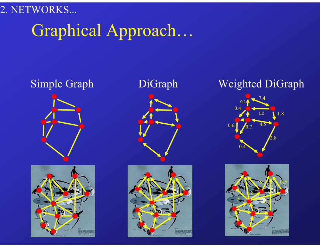
Example: Food WebGOAL: A unified approach

enabling analysis of the

connection topologyconnection topologyunderlying a wide variety of Complex SystemsComplex Systems

2. NETWORKS...

Graphical Approach: Vertices and EdgesExample: Simple graph G with Vertex SetVertex Set V(G)={V1,…,V8}

1 2 3 4 5 6 7 8

1 0 1 1 0 0 0 0 0

2 1 0 1 1 1 0 0 0

3 1 1 0 0 0 1 0 0

4 0 1 0 0 1 0 1 0

5 0 1 0 1 0 1 1 0

6 0 0 1 0 1 0 0 1

7 0 0 0 1 1 0 0 1

8 0 0 0 0 0 1 1 0

Symmetrical Adjacency Matrix Afor the Simple Graph G

V1V2

V4V5 V6

V7V8

V3

Aij = 1 iff (i,j) is in theEdge SetEdge Set E(G)

2. NETWORKS...

Simple Graph

Directed Graph G(DiGraph)

1 2 3 4 5 6 7 8

1 0 0 1 0 0 0 0 0

2 1 0 0 1 0 0 0 0

3 1 1 0 0 0 1 0 0

4 0 0 0 0 0 0 1 0

5 0 1 0 1 0 1 1 0

6 0 0 0 0 1 0 0 1

7 0 0 0 0 0 0 0 1

8 0 0 0 0 0 0 1 0

Non-Symmetrical AdjacencyMatrix A for the DiGraphV1

V4V5 V6

V7V8

Graphical Approach…Aij = 1 iff (i,j) is in the edge set E(G)

V2V3

2. NETWORKS...

28

5

0.58

Simple Graph DiGraph Weighted DiGraph

0.4

0.7 4.5

1.8

2.8

0.6

0.4

7.4

Graphical Approach…

0.1

1.2

2. NETWORKS...

Structural Characterization

Vertex Degree: k(v)Simple Graph

3)( =ke.g. Trade Network

v

v

v

2. NETWORKS...

Clustering Coefficient: C(v)Simple Graph

Structural Characterization…

e.g. Trade Network

v

v

2. NETWORKS...

Clustering Coefficient: C(v)

• Degree of vertex (number of directly connected vertices): k( ) = 3

Simple Graph

Structural Characterization…

e.g. Trade Network

v

v

2. NETWORKS...

Clustering Coeficient: C(v)

• Degree of vertex : k( ) = 3• Total number of possible connections

among these 3 neighbors: ½·k(v)·[k(v)-1] = ½·[3·2] = 3

Simple Graph

Structural Characterization…

e.g. Trade Network

v

v

2. NETWORKS...

Clustering Coefficient: C(v)

• Number of actual connections among the three neighbors = 1

• Total number of possible connections: ½·k(v)·[k(v)-1] = ½·[3·2] = 3

• C(v) = 1 / 3 = 0.33333• Measures how well my neighbors are

connected to each other!

Simple Graph

Structural Characterization…

e.g. Trade Network

v

v

2. NETWORKS...

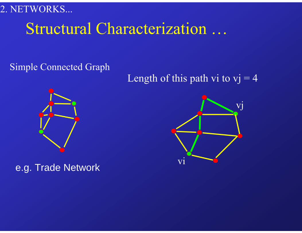
“Distance” vi to vj?Simple Connected Graph

Structural Characterization…

vi

vj

e.g. Trade Network

2. NETWORKS...

Length of this path vi to vj = 4Simple Connected Graph

Structural Characterization …

vi

vj

e.g. Trade Network

2. NETWORKS...

Length of this path vi to vj = 3Simple Connected Graph

Structural Characterization…

vi

vj

e.g. Trade Network

2. NETWORKS...

DistanceDistance vi to vj = ShortestShortest path length vi to vj, here equal to 3Simple Connected Graph

Structural Characterization…

e.g. Trade Networkvi

vj

2. NETWORKS...

Distance from vertex vi to each other vertex v?

Simple Connected Graph

vi

Structural Characterization...

e.g. Trade Network

2. NETWORKS...

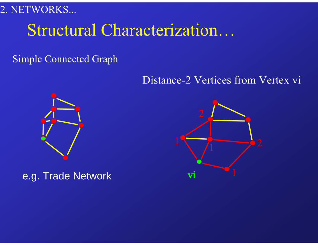
Distance-1 Vertices from Vertex viSimple Connected Graph

1

1

1

Structural Characterization…

e.g. Trade Networkvi

2. NETWORKS...

Distance-2 Vertices from Vertex vi

Simple Connected Graph

vi

1

1

1

2

2

Structural Characterization…

e.g. Trade Network

2. NETWORKS...

Characterization

Distance 3-Vertices from Vertex viSimple Connected Graph

vi

1

1

1

2

2

3

3

DistanceDistance ijL : Length of the shortestshortest path(s) from vi to vj

2. NETWORKS...

• All-to-all distance matrix:Length of the shortest path(s)

1 2 3 4 5 6 7 8 9

1 0 1 1 2 2 2 3 3 4

2 1 0 1 1 1 2 2 3 4

3 1 1 0 2 2 1 3 2 3

4 2 1 2 0 1 2 1 2 3

5 2 1 2 1 0 1 1 2 3

6 2 2 1 2 1 0 2 1 2

7 3 2 3 1 1 2 0 1 2

8 3 3 2 2 2 1 1 0 1

9 4 4 3 3 3 2 2 1 0

L(G) = Characteristic Path Length of Graph G

ijL

L(G)L(G) = Average of Lij over all vertices vi and vj (i ≠ j) in V(G) = 1.94

v7

v4

v9

v8

v1v3

v6

v2

v5

2. NETWORKS...

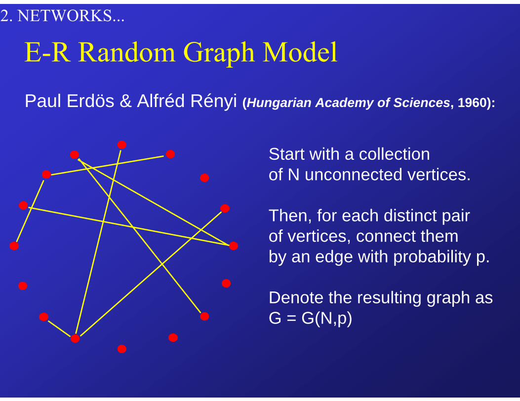
Paul Erdös & Alfréd Rényi (Hungarian Academy of Sciences, 1960):

E-R Random Graph Model

Start with a collection of N unconnected vertices.

Then, for each distinct pairof vertices, connect them by an edge with probability p.

Denote the resulting graph asG = G(N,p)

2. NETWORKS...

• Degree distribution: PG(k)

Poissonian!

E-R Random Graph Model…Continued

PG(k) = Probability that a randomly selected vertex inG will have degree k

PG(k) ~ [ e(-z) zk ]/k! for G=G(N,p)where z = mean k (depends on N,p)

N=1020p = 0.2

2. NETWORKS...

• Regular = Every vertex has the same degree

• |V(G)| = No. of Vertices = 16

• Degree k = 4

• Clustering: C(G) = 1/2

• Characteristic Path Length:

L(G) = 36/15 = 12/5

Graph G for a Regular Ring Lattice

1 1

1 1

2

2 2

33

3 3

4 44

2

vi

2. NETWORKS...

Duncan Watts & Steven Strogatz (Nature, 1998): Small-World Network (SWN) Models

v V*Construction of SWN G(p), 0≤ p≤1

Choose a vertex v and edge e* that connects v to its nearest neighbor v* in clockwise direction.

With probability p, reconnect edge to a vertex v** chosen uniformly at random over the ring but withduplicate edges forbidden.

Continue process clockwise around ring until 1 lap is complete.

e*

v**

e**

2. NETWORKS...

Watts-Strogatz 1998: Construction of Small-World Network G(p)SWN Models…Continued

Rewired edges are called “SHORT-CUTS“

Next consider edges e‘ at distance 2 from from each v in clockwisedirection, and randomly rewirewith probability p.

Moving clockwise, complete a full lap of distance-2 rewiring.

In general, for a ring of any even degree k, successively rewire ALL edges with probability p by completing k/2 laps around ring.

v

V**

e‘

V *V ’

e**

2. NETWORKS...

• For a range of p’s with 0 < p < 1, the SWN G(p) is characterized by– High clustering C(p)/C(0)– Short path length L(p)/L(0)

Watts, Strogatz. Nature 393/4, 1998

Watts-Strogatz 1998: Construction of Small-World Network G(p)

SWN Models…Continued

2. NETWORKS...

• At each step add new vertex v to graph and connect it to 2 randomly selected existing vertices vi using“preferential attachment” prob’s

• Results:– “Richer-Get-Richer”– PG(k) ~ k –3 (Power Law =Scale Free)

Albert-Lázló Barabási (A-B) Scale-Free Network (Science, 1999):

SWN Models…Continued

∑=

jj

ii k

kp = Prob(= Prob(vi)

v

2. NETWORKS...

Properties of the Network ModelsWS Small-WorldRegular E-R RandomAB Small-World

Path length

Clustering

Long Short Short Short

Large Large Large Small

Small-world networks fall “between” regular and E-R random networks!

2. NETWORKS...

Regular Lattice A-B Scale-Free SWN E-R Random Graph

PG(k) = δ(k - kTrue) :Delta Function equals 1 at

true degree k and 0 elsewhere

PG(k) ~ [ e(-z)zk ]/k!z = mean k

Properties of the Network Models…

PG(k) ~ k –3

power law

“thick tailed”

2. NETWORKS...

•• Network Resiliance:Network Resiliance:

–Highly robust against RANDOM failures of vertices v

Small-World Nets: Robustness to Shocks

V

2. NETWORKS...

•• Network Resiliance:Network Resiliance:

–Highly robust against RANDOM failures of vertices v

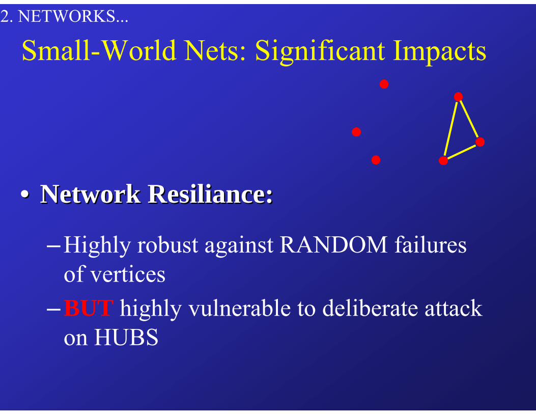
Small-World Nets: Significant Impacts

2. NETWORKS...

•• Network Resiliance:Network Resiliance:

–Highly robust against RANDOM failures of vertices

–BUT highly vulnerable to deliberate attack on HUBS (v’s having a relatively high degree k)

Small-World Nets: Significant ImpactsV

2. NETWORKS...

•• Network Resiliance:Network Resiliance:

–Highly robust against RANDOM failures of vertices

–BUT highly vulnerable to deliberate attack on HUBS

Small-World Nets: Significant Impacts

2. NETWORKS...

So how well do YOU know Kevin Bacon?

• Small-World Effect = Hypothesis that every two people in the world are connected by a surprisingly short chain of social acquaintances.

•• Example:Example: The trivia game Six Degrees of Six Degrees of Kevin BaconKevin Bacon

2. NETWORKS...

Six Degrees of Kevin Bacon…• Name taken from 1990 stage play by American playright

John Guare: Six Degrees of Separation

• Play loosely based on 1967 small-world experiment by Stanley Milgrom suggesting random pairs of U.S. citizens were connected on average by a chain of six social acquaintances (people on a first-name basis).

• Pick any film actor A, then try to link this actor to Bacon via a chain of films.

• Actor set for first film in chain must include A, each successive film must include an actor from previous film, and final film must include Bacon among its actors.

2. NETWORKS...

Six Degrees of Kevin Bacon….

Example:Example: (from Wikipedia, accessed 4/8/07)http://http://en.wikipedia.org/wiki/Six_Degrees_of_Kevin_Baconen.wikipedia.org/wiki/Six_Degrees_of_Kevin_Bacon

Elvis Presley was in Change of Habit (1969) with Edward Asner

Edward Asner was in JFK (1991) with Kevin Bacon

Therefore Elvis Presley has a Bacon Number = 2.

2. NETWORKS...

Rank Name Averagedistance

# ofmovies

# oflinks

1 Rod Steiger 2.537527 112 25622 Donald Pleasence 2.542376 180 28743 Martin Sheen 2.551210 136 35014 Christopher Lee 2.552497 201 29935 Robert Mitchum 2.557181 136 29056 Charlton Heston 2.566284 104 25527 Eddie Albert 2.567036 112 33338 Robert Vaughn 2.570193 126 27619 Donald Sutherland 2.577880 107 2865

10 John Gielgud 2.578980 122 294211 Anthony Quinn 2.579750 146 297812 James Earl Jones 2.584440 112 3787…

876 Kevin Bacon 2.786981 46 1811…

What’s the average distance between Kevin Bacon and all other actors?(from Albert-Lázló Barabási , www.nd.edu/~networks)

No. of movies : 46 No. of actors : 1811 Average separation: 2.79Kevin Bacon

Is Kevin Bacon the most

connected actor?

NO!

876 Kevin Bacon 2.786981 46 1811