Structural Dynamic Capabilities of ANSYS

Erke Wang, Thomas Nelson

CADFEM GmbH, Munich, Germany

Abstract: ANSYS is one of the leading commercial finite element programs in the world and can be applied to a large number of applications in engineering. Finite element solutions are available for several engineering disciplines like statics, dynamics, heat flow, fluid flow, electromagnetics and also coupled field problems. In the present paper we summarize the current simulation capabilities of ANSYS in structural dynamics. A general classification of dynamical problems that can be solved with ANSYS is given considering not only the implicit but also the explicit solution capabilities of the code.

A useful feature of ANSYS that is not only available for problems in structural dynamics are the ANSYS Parametric Design Language (APDL) that enables the user to completely parametrize the model. With parametric modelling the investigation of results due to a variation of the input parameters can be done quite comfortably.

Considering the solution speed of eigenvalue problems we focus on a few quite powerful eigenvalue solver available in ANSYS especially the QR Damped Method and the Powerdynamics Method that decrease the required solution time significantly.

To show the general development of ANSYS into an easy-to-use software we finally present the drop test module of ANSYS which enables the user to perform any drop test in a most comfortable way.

Introduction The finite element method (FEM) is the most popular simulation method to predict the physical behaviour of systems and structures. Since analytical solutions are in general not available for most daily problems in engineering sciences numerical methods have been evolved to find a solution for the governing equations of the individual problem. Although the finite element method was originally developed to find a solution for problems of structural mechanics it can nowadays be applied to a large number of engineering disciplines in which the physical description results in a mathematical formulation with some typical differential equations that can be solved numerically.

Much research work has been done in the field of numerical modelling during the last twenty years which enables engineers today to perform simulations close to reality. Nonlinear phenomena in structural mechanics such as nonlinear material behaviour, large deformations or contact problems have become standard modelling tasks. Because of a rapid development in the hardware sector resulting in more and more powerful processors together with decreasing costs of memory it is nowadays possible to perform simulations even for models with millions of degrees of freedom.

ANSYS provides finite element solutions for several engineering disciplines like statics, dynamics, heat flow, fluid flow, electromagnetics and also coupled field problems. The ANSYS user is able to run simulations for linear and nonlinear problems in engineering where structural nonlinearities may occur due to nonlinear material behaviour, large deformations or contact boundary conditions.

CAD-FEM GmbH is the official ANSYS distributor for Germany, Austria and Switzerland and has an experienced team of engineers that performs numerical simulations for industry covering all engineering disciplines mentioned above. CAD-FEM GmbH also provides technical support for all ANSYS customers of the above countries. For education purposes, many professional seminars are offered ranging from introductory courses to courses covering highly advanced topics of numerical modelling techniques.

With this paper, we give an overview of the present capabilities of ANSYS in the field of structural dynamics. A general classification of dynamical calculation disciplines will be provided. The algorithms that are available with the present version of ANSYS are discussed together with their typical applications. Considering the time integration method for transient problems we emphasize implicit and explicit solution capabilities of ANSYS. Furthermore, we focus on algorithms that reduce the solution time of dynamical calculations significantly. Two methods will be discussed in detail: First of all, to determine the natural frequencies of very large models where typically solid elements are used ANSYS provides an algorithm called Powerdynamics Method which shows quite good results when comparing the solution time with other classical algorithms. In addition, the QR Damped Method is introduced which enables the user to model non-proportional damping not only in a modal analysis but also in a transient and harmonic analysis when based on the modal superposition technique. Again this results in less computation time. We also will mention how damping can be modelled in ANSYS. With the modern ANSYS Parametric Design Language (APDL) the user is able to model its problem in a parametric way. Furthermore, several mathematical operations are available for postprocessing purposes. Finally, we present some numerical examples of structural dynamics including a drop test of a personal digital assistant as an example of explicit transient dynamics performed with the easy-to-use drop test module of ANSYS.

Problems of Structural Dynamics - Numerical Methods in ANSYS In this chapter we give a general overview of typical problems in structural dynamics. Based on d’Alemberts principle and due to the discretization process of a continuous structure with finite elements the following equation of motion can be derived:

)((t) 1fuKuCuM =⋅+⋅+⋅ &&&

In the above equation and ,M C K denote the structural mass, damping and stiffness matrices. The vectors of nodal accelerations, velocities and displacements are u& and u respectively. ,& u& (t)f is the vector of applied forces. Dynamical equilibrium is obtained if equation (1) holds for all times .t

All problems in structural dynamics can be formulated based on the above equation of motion (1). A coarse classification is obtained by taking different representations for the time varying applied forces. For this classification Figure 1 presents a diagram where several analysis types of structural dynamics are listed according to the representation of the applied load.

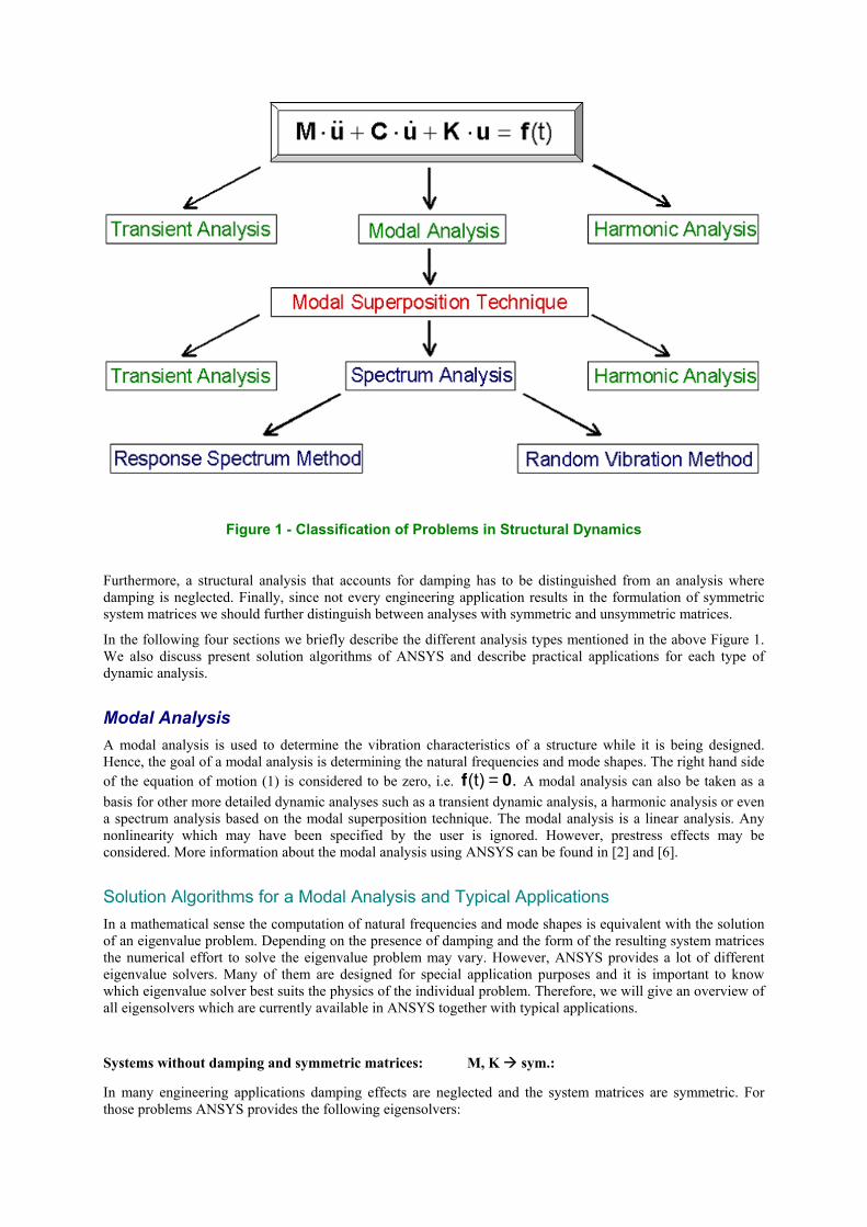
Figure 1 - Classification of Problems in Structural Dynamics

Furthermore, a structural analysis that accounts for damping has to be distinguished from an analysis where damping is neglected. Finally, since not every engineering application results in the formulation of symmetric system matrices we should further distinguish between analyses with symmetric and unsymmetric matrices.

In the following four sections we briefly describe the different analysis types mentioned in the above Figure 1. We also discuss present solution algorithms of ANSYS and describe practical applications for each type of dynamic analysis.

Modal Analysis A modal analysis is used to determine the vibration characteristics of a structure while it is being designed. Hence, the goal of a modal analysis is determining the natural frequencies and mode shapes. The right hand side of the equation of motion (1) is considered to be zero, i.e. .(t) 0f = A modal analysis can also be taken as a basis for other more detailed dynamic analyses such as a transient dynamic analysis, a harmonic analysis or even a spectrum analysis based on the modal superposition technique. The modal analysis is a linear analysis. Any nonlinearity which may have been specified by the user is ignored. However, prestress effects may be considered. More information about the modal analysis using ANSYS can be found in [2] and [6].

Solution Algorithms for a Modal Analysis and Typical Applications In a mathematical sense the computation of natural frequencies and mode shapes is equivalent with the solution of an eigenvalue problem. Depending on the presence of damping and the form of the resulting system matrices the numerical effort to solve the eigenvalue problem may vary. However, ANSYS provides a lot of different eigenvalue solvers. Many of them are designed for special application purposes and it is important to know which eigenvalue solver best suits the physics of the individual problem. Therefore, we will give an overview of all eigensolvers which are currently available in ANSYS together with typical applications.

Systems without damping and symmetric matrices: M, K sym.:

In many engineering applications damping effects are neglected and the system matrices are symmetric. For those problems ANSYS provides the following eigensolvers:

• Block Lanczos Method

• Subspace Method

• Reduced Method

• Powerdynamics Method

The Block Lanczos Method is a very efficient algorithm to perform a modal analysis for large models. It is a fast and robust algorithm and used for most applications as the default solver.

The Subspace Method was popular in earlier years since very little computer resources were necessary to perform a modal analysis. However, compared with the Block Lanczos Method the Subspace Method is fast for small models but solution time increases as soon as larger models are considered.

The Reduced Method is also an old eigensolver which works with reduced matrices in order to minimize the number of dynamic degrees of freedom. Master degrees of freedom have to be chosen which represent the dynamic response of the system as accurately as possible. Neither the Subspace Method nor the Reduced Method are popular today.

The Powerdynamics Method is a special algorithm based on the Subspace Method. During the Subspace Algorithm linear systems of equations have to be solved. For this purpose, ANSYS provides several equation solver. Typical solver for problems in structural mechanics are the Sparse Solver, the Frontal Solver and the Pre-conditioned Conjugate Gradient Solver (PCG-Solver). Each of these equation solver has its special characteristics. At this stage we focus especially on the Frontal Solver and the PCG-Solver since both can be used within the Subspace Method. By default the Subspace Method as mentioned above uses the Frontal Solver to obtain the first natural frequencies of a structure. This solver works efficiently for small models of up to 50,000 active degrees of freedom. However, if models consist mainly of solid elements with more than 50,000 active degrees of freedom, the Subspace Method combined with the PCG-Solver should be the preferred solution method. In ANSYS the combination of the Subspace Method together with the PCG-Solver is called Powerdynamics Method. For large models of up to 10,000,000 degrees of freedom, this method significantly reduces solution time. Another characteristic of the Powerdynamics Method is the lumped mass matrix formulation. In a lumped mass approach, the mass matrix is diagonal since the mass is considered concentrated at the nodes. Note that the Subspace Method is the only eigensolver in ANSYS where the user has the option to specify the equation solver.

Systems without damping and unsymmetric matrices: M, K unsym.:

Some engineering applications in which structural damping is ignored may lead to unsymmetric system matrices. In those cases the ANSYS user can take advantage of the following eigensolver called:

• Unsymmetric Method

In fact, this method uses a Lanczos algorithm to solve the resulting unsymmetric eigenvalue problem which is commonly encountered in fluid-structure-interaction problems.

For example if interest lies in the natural frequencies of a steel ring which is submerged in a compressible fluid the matrices are unsymmetric and the user has to apply the Unsymmetric Method as an appropriate eigensolver.

Damped systems with symmetric matrices: M, K sym., C sym.:

If damping is considered and the system matrices are symmetric, the user can choose the following eigensolver to calculate damped natural frequencies of a structure:

• QR Damped Method

The QR Damped Method typically consists of two parts: First, the Block Lanczos Method mentioned earlier in this section is used to compute the solution of the undamped system. Hence, all natural frequencies and mode shapes will be calculated for zero damping. Note that the Block Lanczos Method ignores the damping matrix even if it is set up by the program.

In a second step, the equation of motion now including the damping matrix is transformed with the matrices of undamped mode shapes into the modal subspace. This procedure is identical with the first step of the modal superposition technique which will be discussed in the next subsection. After some further mathematical manipulations an extended eigenvalue problem can be formulated. The resulting eigenvalues of this problem are complex. Each real part of an eigenvalue physically represents the damping coefficient multiplied with the undamped natural frequency of the considered mode whereas the imaginary part consists of the damped natural frequency itself.

Let us briefly summarize the main properties of the QR Damped Method as an eigensolver: Damped natural frequencies are computed as well as modal damping coefficients of each mode. However, the effects of damping are not considered for the computation of the resulting mode shapes which simply means that only undamped mode shapes are obtained. Furthermore, we should mention that the QR Damped Method gives reasonable results only if undercritical damping is specified. Considering the solution speed the QR Damped Method shows a better performance especially when compared with the Damped Method which will be discussed next.

Damped systems with symmetric/unsymmetric matrices: M, K sym., C sym./unsym.:

Let us assume damping is considered and the resulting damping matrix is either symmetric or unsymmetric. For such applications ANSYS provides the eigensolver called:

• Damped Method

This method accounts for the damping matrix for the formulation of the considered eigenvalue problem. From a mathematical point of view this results in a so called quadratic eigenvalue problem. The obtained eigenvalues are again complex. The real part physically represents the product of the modal damping coefficient and the undamped natural frequency. The imaginary part, however, obtains the damped natural frequency.

In contrast to the QR Damped Method the effect of damping is also considered for the computation of mode shapes which has the consequence that all mode shapes are obtained in a complex form. Therefore, the dynamic response in each mode consists of a real and an imaginary part.

In summary, we note that the Damped Method computes the damped natural frequencies and the real and imaginary parts of each mode shape. Considering solution time, the Damped Method works less efficiently compared with the QR Damped Method described above.

Finally, we discuss in which engineering discipline a symmetric damping matrix is obtained and in which case the damping matrix appears as an unsymmetric one. The modal analysis of damped systems which are at rest leads in general to a symmetric formulation of the resulting damping matrix. Different possibilities to model the effect of damping will be summarized later on in this paper. However, if a modal analysis of a spinning structure has to be performed the effect of the resulting gyroscopic forces has to be included. Indeed these effects are physically comparable with structural damping and therefore a so called gyroscopic matrix has to be set up. In the equation of motion (1) it typically occurs at the same position where usually the damping matrix can be found. It should be noted that for problems involving such rotordynamic stability this gyroscopic matrix is usually unsymmetric. Hence, the Damped Method has to be chosen to perform the analysis.

Modal Superposition Technique for Problems in Structural Dynamics At this stage we would like to describe briefly the modal superposition technique since it is based on a modal analysis which has been discussed so far in this section. Many solution disciplines of structural dynamics require a transient or harmonic analysis that can be performed efficiently when the modal superposition technique is used. Also remember the fact that the spectrum analysis always uses the modal superposition as a basic concept.

We refer to Figure 1 where the important role of the modal superposition technique is shown in context with classical solution disciplines of structural dynamics.

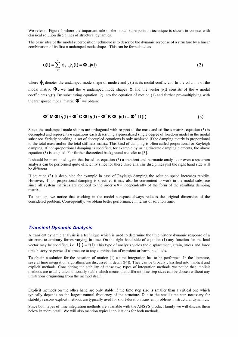
The basic idea of the modal superposition technique is to describe the dynamic response of a structure by a linear combination of its first n undamped mode shapes. This can be formulated as

)((t)(t)(t) 2yΦu ⋅=⋅=∑=

i

n

1ii yϕ

where iϕ denotes the undamped mode shape of mode i and yi(t) is its modal coefficient. In the columns of the

modal matrix , we find the n undamped mode shapes Φ iϕ and the vector y(t) consists of the n modal coefficients yi(t). By substituting equation (2) into the equation of motion (1) and further pre-multiplying with the transposed modal matrix Φ we obtain: T

)((t)(t)(t)(t) 3fΦyΦKΦyΦCΦyΦMΦ ⋅=⋅+⋅+⋅ TTTT &&&

Since the undamped mode shapes are orthogonal with respect to the mass and stiffness matrix, equation (3) is decoupled and represents n equations each describing a generalized single degree of freedom model in the modal subspace. Strictly speaking, a set of decoupled equations is only achieved if the damping matrix is proportional to the total mass and/or the total stiffness matrix. This kind of damping is often called proportional or Rayleigh damping. If non-proportional damping is specified, for example by using discrete damping elements, the above equation (3) is coupled. For further theoretical background we refer to [3].

It should be mentioned again that based on equation (3) a transient and harmonic analysis or even a spectrum analysis can be performed quite efficiently since for these three analysis disciplines just the right hand side will be different.

If equation (3) is decoupled for example in case of Rayleigh damping the solution speed increases rapidly. However, if non-proportional damping is specified it may also be convenient to work in the modal subspace since all system matrices are reduced to the order n×n independently of the form of the resulting damping matrix.

To sum up, we notice that working in the model subspace always reduces the original dimension of the considered problem. Consequently, we obtain better performance in terms of solution time.

Transient Dynamic Analysis A transient dynamic analysis is a technique which is used to determine the time history dynamic response of a structure to arbitrary forces varying in time. On the right hand side of equation (1) any function for the load vector may be specified, i.e. (t).(t) ff = This type of analysis yields the displacement, strain, stress and force time history response of a structure to any combination of transient or harmonic loads.

To obtain a solution for the equation of motion (1) a time integration has to be performed. In the literature, several time integration algorithms are discussed in detail ([4]). They can be broadly classified into implicit and explicit methods. Considering the stability of these two types of integration methods we notice that implicit methods are usually unconditionally stable which means that different time step sizes can be chosen without any limitations originating from the method itself.

Explicit methods on the other hand are only stable if the time step size is smaller than a critical one which typically depends on the largest natural frequency of the structure. Due to the small time step necessary for stability reasons explicit methods are typically used for short-duration transient problems in structural dynamics.

Since both types of time integration methods are available with the ANSYS product family we will discuss them below in more detail. We will also mention typical applications for both methods.

Implicit Time Integration and its Typical Application The implicit time integration algorithm in ANSYS is the Newmark method ([4]). The stability of this method is controlled by two parameters that are set up by default so that the scheme is unconditionally stable and the effect of numerical damping is minimized. Applying the Newmark method to the equation of motion (1) results in a linear system of equation for each time step. Since the stiffness matrix appears on the left hand side it must be inverted in each time step in the incremental solution process. Since its inversion is computationally expensive especially for highly nonlinear problems the implicit solution technique in ANSYS is always a good choice to solve a transient analysis if the problem is not crucially dominated by nonlinearities. More details about the implicit transient analysis using ANSYS are provided in [2] and [6].

To solve a transient analysis ANSYS provides different solution options which will be discussed according to their importance and computational efficiency in more or less detail:

• Full Method

• Reduced Method

• Modal Superposition Method

The Full Method does not reduce the dimension of the considered problem since original matrices are used to compute the solution. As a consequence it is simple to use, all kinds of nonlinearities may be specified, automatic time stepping is available, all kinds of loads may be specified, masses are not assumed to be concentrated at the nodes and finally all results are computed in a single calculation. The main disadvantage of the Full Method is the fact that the required solution time will increase with the size of the considered model.

The Reduced Method originates from earlier years. Because of the reduced system matrices which are used to solve the transient problem, this method has an advantage when compared with the Full Method with respect to the required solution time. However, the user has to specify master degrees of freedom which represent the dynamic behaviour as good as possible. The only nonlinearity which can be specified is node-to-node contact via a gap condition. However, automatic time stepping is not possible. Consequently, this method is not very popular any more since all its disadvantages do not really compensate the advantage of lower costs in solution time.

The Modal Superposition Method usually reduces the dimension of the original problem as well since the transient analysis is finally performed in the modal subspace which has the dimension of the number of mode shapes used for the superposition. The main advantage is again the reduction of solution time. It turns out that this method is actually the most efficient one compared with the other two. The accuracy just depends on the number of mode shapes used for the modal superposition. Even if a few modes shapes are taken the requested solution time might still be less when compared with the Full and the Reduced Method. Contact can be applied using the gap condition we mentioned in the discussion of the Reduced Method. The time step has to be chosen as constant which means that automatic time stepping is not available for this method. It should also be noted that a modal analysis has to be performed before the transient problem can be solved with the modal superposition technique. Hence, the solution process consists basically of two analyses, the modal analysis and the transient analysis in the modal subspace. Since for most problems in structural dynamics the natural frequencies of a structure are of interest this is not really a disadvantage. Summing up, using the modal superposition technique for a transient analysis reduces not only solution time, but the user also obtains information about the natural frequencies and the undamped mode shapes, respectively.

Comparing the above solution options the Modal Superposition Method is the most powerful method considering the required solution time. However, it cannot handle nonlinearities. The Full Method requires more time to finish the analysis but can handle nonlinearities.

Explicit Time Integration and its Typical Application ANSYS also provides the possibility to perform an explicit transient analysis. ANSYS/LS-DYNA as a product of the ANSYS family combines the LS-DYNA explicit finite element solver with the powerful pre- and postprocessing capabilities of ANSYS.

As an explicit time integration algorithm, LS-DYNA uses a central difference scheme ([4]). Similarly as the implicit Newmark method linear systems of equation have to be solved in each time step. However, the stiffness matrix will appear on the right hand side during the solution process and therefore does not need to be inverted in each step. For this reason ANSYS/LS-DNYA can handle highly nonlinear problems in transient dynamics

very well. Fast solution capabilities are provided for short-time large deformation dynamics, quasi-static problems with large deformations and multiple nonlinearities and also for complex contact/impact problems. For highly nonlinear transient problems the product ANSYS/LS-DYNA might be the better choice compared with ANSYS in its implicit version. More details about ANSYS/LS-DYNA can be found in [1].

Because of the small time step which has usually to be taken for stability reasons in ANSYS/LS-DYNA long-time transient problems might run inefficiently with this code and ANSYS in its implicit form could be a better choice.

With ANSYS/LS-DYNA, the user can perform the complete preprocessing in ANSYS, obtain the explicit dynamic solution via LS-DYNA and review the results using again the ANSYS postprocessing tools the user might be already familiar with. It is also possible to transfer geometry and result information between ANSYS and ANSYS/LS-DYNA to perform a sequential implicit-explicit/explicit-implicit analysis, such as required for a drop test or a springback analysis.

Harmonic Response Analysis Any sustained cyclic load will produce a sustained cyclic response in a structure which is often called a harmonic response. The harmonic response analysis solves the equation of motion (1) for linear structures undergoing steady-state vibrations. All loads and displacements vary sinusoidally with the same known frequency although not necessarily in phase. The use of a complex notation allows a compact and efficient description of the problem. For the function of applied force on the right hand side of the equation of motion (1) the following expression is used, i.e. . In this formulation represents the amplitude

of the force, Ω denotes the imposed circular frequency measured in radians/time and stands for the force phase shift which is measured in radians. For additional information we refer to [2] and [6].

)(e(t) Ψ+Ω⋅= timaxff maxf

Ψ

As for the transient dynamic analysis ANSYS provides several solution options to solve a harmonic response analysis which will be discussed more or less in detail according to their immediate meaning:

• Full Method

• Reduced Method

• Modal Superposition Method

Note that the same three solution methods which are available for the transient dynamic analysis are provided to perform a harmonic response analysis. Since the mean characteristics of these methods have been already explained earlier we will not repeat them at this stage. All discussed advantages and disadvantages remain the same if the above methods are applied to a harmonic response analysis. Some features which are typical for these methods when used in the harmonic response analysis are discussed as follows.

One feature of the Full Method which should be mentioned here is the capability of handling unsymmetric matrices which occur in problems of fluid-structure-interaction or rotordyamics. However, considering the solution time the Reduced Method and the Modal Superposition Method will still provide better performance, but cannot handle unsymmetric matrices.

The Reduced Method and the Modal Superposition Method have the capability to take into consideration the effects of pre-stressing within a harmonic analysis. With the general improvement in solution time this turns out as an advantage when compared with the Full Method. Nevertheless, the Modal Superposition Method itself shows the best performance when observing the solution time.

Spectrum Analysis A spectrum analysis is a dynamical calculation discipline in which the results of a modal analysis are used together with a well-known spectrum to calculate certain quantities in the structure like displacements and stresses for example. A spectrum is simply a graph of a spectral quantity like the acceleration versus frequency that captures the intensity and frequency content of time-history loads.

The spectrum analysis is often used instead of a transient dynamic analysis to determine the response of structures due to random or time-dependent loading conditions such as earthquakes, wind loads, ocean wave

loads, jet engine thrusts, rocket motor vibrations and so on. Contrary to a transient analysis a spectrum analysis does not calculate the dynamic answer for the whole considered time range where the dynamic forces have been acting. Rather a conservative estimation for the maximum response of a certain quantity like the displacements or stresses is obtained from this type of analysis. Additional information about the spectrum analysis can be found in [2] and [6].

To discuss further aspects of a spectrum analysis we should distinguish the deterministic way of consideration from the non-deterministic one. Up to now each analysis type has been of a deterministic nature since the load function has been always a clearly defined one. This assumption holds for the most engineering applications of today. Strictly speaking, dynamic loads appear quite often to be statistical in nature and hence a non-deterministic probabilistic consideration could be even more suitable. In the following two subsections we provide detailed information about the deterministic response spectrum analysis and the non-deterministic random vibration analysis.

Deterministic Response Spectrum Analysis For the deterministic response spectrum analysis the following types of spectra are available in ANSYS and we will try to explain their main characteristics as follows:

• Response Spectrum

Single-point Response Spectrum

Multi-point Response Spectrum

• Dynamic Design Analysis Method

A response spectrum represents the response of a single degree of freedom system to a time-history loading function. It is a graph of response versus frequency where the response might be a displacement, velocity, acceleration, or even a force. In a single-point response spectrum analysis you specify one response spectrum curve at a set of points in the model, such as at all supports. On the other hand, in a multi-point response spectrum analysis you specify different spectrum curves at different sets of points.

The dynamic design analysis method is a technique used to evaluate the shock resistance of shipboard equipment. The technique is essentially a response spectrum analysis in which the spectrum is obtained from a series of empirical equations and shock design tables provided in the U.S. Naval Research Laboratory Report NRL-1396.

Non-deterministic Random Vibration Analysis For the non-deterministic random vibration analysis the following type of spectrum is used in ANSYS:

• Power Spectral Density (PSD)

PSD is a statistical measure defined as the limiting mean-square value of a random variable. It is used in a random vibration analysis in which the instantaneous magnitudes of the response can be specified only by a probability distribution function that shows the probability of the magnitude taking a particular value. A PSD is a statistical measure of the response of a structure to random dynamic loading conditions. It is a graph of the PSD value versus frequency where the PSD may be a displacement PSD, velocity PSD, acceleration PSD, or a force PSD. Mathematically spoken, the area under a PSD-versus-frequency curve is equal to the variance that is simply the square of the standard deviation of the response.

Similarly to the response spectrum analysis a random vibration analysis may be single-point or even multi-point. In a single-point random vibration analysis you specify one PSD spectrum at a set of points. In a multi-point random vibration analysis, you specify different PSD spectra at different points.

Various Possibilities to Model the Effect of Damping in ANSYS In nature, every dynamic process is subjected to the effect of damping. A totally undamped vibration actually does not exist in reality. In ANSYS, there are several possibilities available to model the effect of structural damping. The aim of this chapter is to give an overview of currently existing damping models of ANSYS. Since not every kind of damping can be applied in each solution method that is available for the different calculation disciplines, we have to discuss which damping model can be used in which solution method.

Assuming that the damping matrix in the equation of motion (1) is set up directly and no transformation into the modal subspace is performed the following formulation can be given taken from [3]:

)(4∑∑==

+⋅+⋅+⋅+⋅=NEL

1jjc

NMAT

1iii βββα CKKKMC

14243 14243 123 123

1 2 3 4

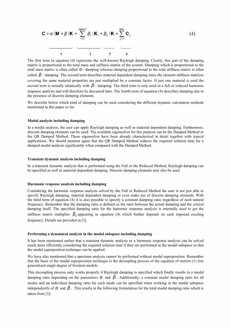
The first term in equation (4) represents the well-known Rayleigh damping. Clearly, this part of the damping matrix is proportional to the total mass and stiffness matrix of the system. Damping which is proportional to the total mass matrix is often called α - damping whereas damping proportional to the total stiffness matrix is often called - damping. The second term describes material dependent damping since the element stiffness matrices covering the same material properties are just multiplied by a constant factor. If just one material is used the second term is actually identically with - damping. The third term is only used in a full or reduced harmonic response analysis and will therefore be discussed later. The fourth term of equation (4) describes damping due to the presence of discrete damping elements.

β

β

We describe below which kind of damping can be used considering the different dynamic calculation methods mentioned in this paper so far:

Modal analysis including damping

In a modal analysis, the user can apply Rayleigh damping as well as material dependent damping. Furthermore, discrete damping elements can be used. The available eigensolver for this purpose can be the Damped Method or the QR Damped Method. These eigensolver have been already characterized in detail together with typical applications. We should mention again that the QR Damped Method reduces the required solution time for a damped modal analysis significantly when compared with the Damped Method.

Transient dynamic analysis including damping

In a transient dynamic analysis that is performed using the Full or the Reduced Method, Rayleigh damping can be specified as well as material dependent damping. Discrete damping elements may also be used.

Harmonic response analysis including damping

Considering the harmonic response analysis solved by the Full or Reduced Method the user is not just able to specify Rayleigh damping, material dependent damping or even make use of discrete damping elements. With the third term of equation (4) it is also possible to specify a constant damping ratio regardless of each natural frequency. Remember that the damping ratio is defined as the ratio between the actual damping and the critical damping itself. The specified damping ratio for the harmonic response analysis is internally used to get the stiffness matrix multiplier appearing in equation (4) which further depends on each imposed exciting frequency. Details are provided in [3].

cβ

Performing a dynamical analysis in the modal subspace including damping

It has been mentioned earlier that a transient dynamic analysis or a harmonic response analysis can be solved much more efficiently considering the required solution time if they are performed in the modal subspace so that the modal superposition technique can be applied.

We have also mentioned that a spectrum analysis cannot be performed without modal superposition. Remember that the basis of the modal superposition technique is the decoupling process of the equation of motion (1) into generalized single degree of freedom models.

This decoupling process only works properly if Rayleigh damping is specified which finally results in a modal damping ratio depending on the parameters α and . Additionally, a constant modal damping ratio for all modes and an individual damping ratio for each mode can be specified when working in the modal subspace independently of and . This results in the following formulation for the total modal damping ratio which is taken from [3]:

β

α β

)(5mii

ii ξξ

2ωβ

ω2αξ ++⋅+⋅

=

144424443 123 123

1 2 3

In equation (5) the first term represents α - and - damping. The second one describes the constant modal damping ratio used for all modes and the third term represents the individual modal damping ratio which can be prescribed for each single mode differently.

β

It has been mentioned already that it is quite convenient to perform a dynamic analysis in the modal subspace since the dimension of the problem is reduced according to the number of mode shapes you consider. However, the modal superposition technique in its classical form cannot take into account the effects of non-proportional damping, i.e. when material dependent damping is used or discrete damping elements are present. In such a case the decoupling process of the resulting damping matrix does not work properly.

Nevertheless, if the user wants to apply non-proportional damping but also likes to take advantage of working in the modal subspace ANSYS provides a special method to do this. The modal analysis has to be done by using the QR Damped Method as an eigensolver. Every kind of non-proportional damping can be considered further in a transient, harmonic or in a spectrum analysis when performed in the modal subspace. Hence, the QR Damped Method does not just reduce the solution time in a modal analysis. It also enables the user to work in the modal subspace with non-proportional damping which results again in a better performance considering the solution speed.

Parametric Modelling and Efficient Postprocessing using APDL In this chapter, we introduce the ANSYS Parametric Design Language (APDL) as a useful capability to build up a model in a parametric way. Also various mathematical operations are available for postprocessing purposes which are especially useful if the obtained results have further to be manipulated in a mathematical sense. We explain basic characteristics and features of the ANSYS Parametric Design Language (APDL) by showing simple examples.

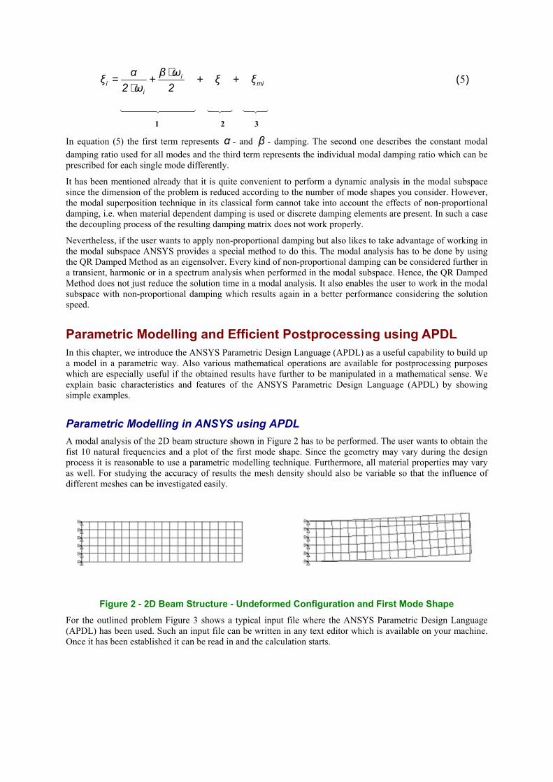
Parametric Modelling in ANSYS using APDL A modal analysis of the 2D beam structure shown in Figure 2 has to be performed. The user wants to obtain the fist 10 natural frequencies and a plot of the first mode shape. Since the geometry may vary during the design process it is reasonable to use a parametric modelling technique. Furthermore, all material properties may vary as well. For studying the accuracy of results the mesh density should also be variable so that the influence of different meshes can be investigated easily.

Figure 2 - 2D Beam Structure - Undeformed Configuration and First Mode Shape For the outlined problem Figure 3 shows a typical input file where the ANSYS Parametric Design Language (APDL) has been used. Such an input file can be written in any text editor which is available on your machine. Once it has been established it can be read in and the calculation starts.

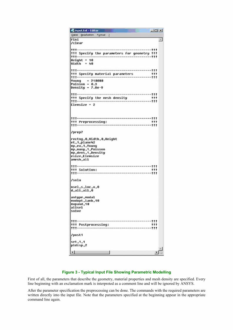
Figure 3 - Typical Input File Showing Parametric Modelling First of all, the parameters that describe the geometry, material properties and mesh density are specified. Every line beginning with an exclamation mark is interpreted as a comment line and will be ignored by ANSYS.

After the parameter specification the preprocessing can be done. The commands with the required parameters are written directly into the input file. Note that the parameters specified at the beginning appear in the appropriate command line again.

After finishing the preprocessing we enter the solution part. First of all, the nodes at the location X = 0 are selected to apply the boundary conditions of a fixed edge. As analysis type the modal analysis is chosen with the Block Lanczos Method as an eigensolver. The first 10 modes should be calculated together with the mode shapes.

During the postprocessing the user asks to plot the displacements of the first mode shape together with the edge of the undeformed configuration.

It is quite obviously that parametric studies can be performed easily using APDL. The user just changes the value of a parameter and reads in the input file again.

Many other capabilities of APDL are not shown in the input file of Figure 3. For example, like in any other programming language it is possible to program do-loops as well as if-else-conditions, etc.

To sum up, APDL provides a very powerful capability to the user since the complete simulation can be done automatically beginning with preprocessing and ending with postprocessing.

Mathematical Operations for Effective Postprocessing using APDL As mentioned earlier for some applications of structural dynamics the obtained results might be complex. For example a damped modal analysis results in complex mode shapes and a real and imaginary part of each mode shape is obtained. The dynamic answer consists of both parts and can be computed using the following equation taken from [6]

)(t)sintcos(e(t) t 6DimDreδ ωω ϕϕ −= −u

where reϕ and imϕ denote the real and imaginary part of the considered mode shape, Dω stands for the

damped natural frequency and δ covers the product of modal damping ratio and undamped natural frequency. Clearly, u is the resulting displacement vector depending on the physical time .tFigure 4 shows a subroutine which could be read in during the postprocessing to compute a damped mode shape of a structure according to equation (4).

Strictly speaking, just the term in brackets of equation (4) has been programmed since this part describes the resulting shape of the vibration. The term with the exponential function just measures the decreasing amplitude of the mode shape.

In the subroutine the considered load- and substep has first to be specified, to describe the interesting mode. After defining π a do-loop in range 0 < t < 2π with an incremental step of π/20 is set up to obtain the values of the used trigonometric functions.

We are of the opinion that the comments state clearly where the mathematical multiplication is performed so we will not provide any more details at this stage.

Note that with APDL many mathematical operations can be performed in ANSYS and no additional program is necessary for further postprocessing.

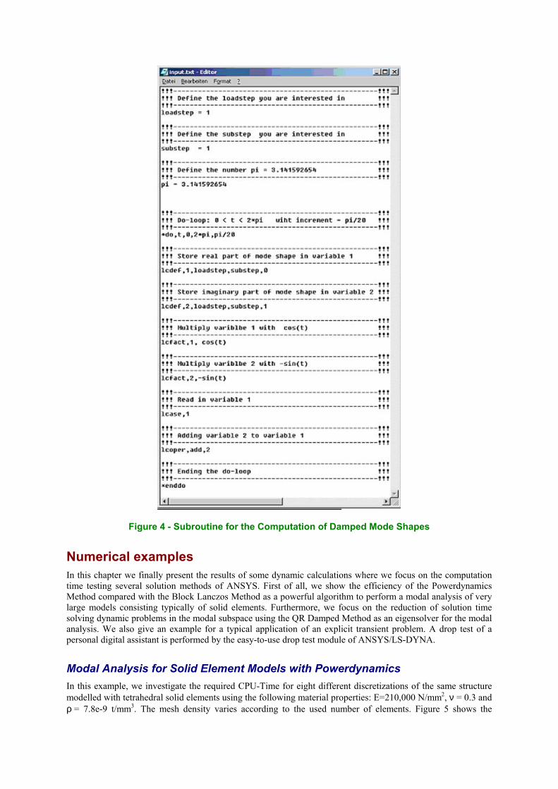
Figure 4 - Subroutine for the Computation of Damped Mode Shapes

Numerical examples In this chapter we finally present the results of some dynamic calculations where we focus on the computation time testing several solution methods of ANSYS. First of all, we show the efficiency of the Powerdynamics Method compared with the Block Lanczos Method as a powerful algorithm to perform a modal analysis of very large models consisting typically of solid elements. Furthermore, we focus on the reduction of solution time solving dynamic problems in the modal subspace using the QR Damped Method as an eigensolver for the modal analysis. We also give an example for a typical application of an explicit transient problem. A drop test of a personal digital assistant is performed by the easy-to-use drop test module of ANSYS/LS-DYNA.

Modal Analysis for Solid Element Models with Powerdynamics In this example, we investigate the required CPU-Time for eight different discretizations of the same structure modelled with tetrahedral solid elements using the following material properties: E=210,000 N/mm2, ν = 0.3 and ρ = 7.8e-9 t/mm3. The mesh density varies according to the used number of elements. Figure 5 shows the

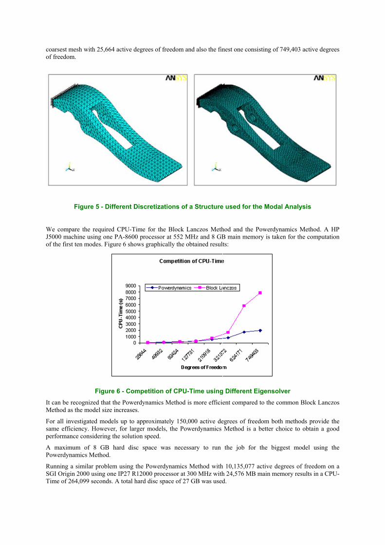
coarsest mesh with 25,664 active degrees of freedom and also the finest one consisting of 749,403 active degrees of freedom.

Figure 5 - Different Discretizations of a Structure used for the Modal Analysis

We compare the required CPU-Time for the Block Lanczos Method and the Powerdynamics Method. A HP J5000 machine using one PA-8600 processor at 552 MHz and 8 GB main memory is taken for the computation of the first ten modes. Figure 6 shows graphically the obtained results:

Figure 6 - Competition of CPU-Time using Different Eigensolver It can be recognized that the Powerdynamics Method is more efficient compared to the common Block Lanczos Method as the model size increases.

For all investigated models up to approximately 150,000 active degrees of freedom both methods provide the same efficiency. However, for larger models, the Powerdynamics Method is a better choice to obtain a good performance considering the solution speed.

A maximum of 8 GB hard disc space was necessary to run the job for the biggest model using the Powerdynamics Method.

Running a similar problem using the Powerdynamics Method with 10,135,077 active degrees of freedom on a SGI Origin 2000 using one IP27 R12000 processor at 300 MHz with 24,576 MB main memory results in a CPU-Time of 264,099 seconds. A total hard disc space of 27 GB was used.

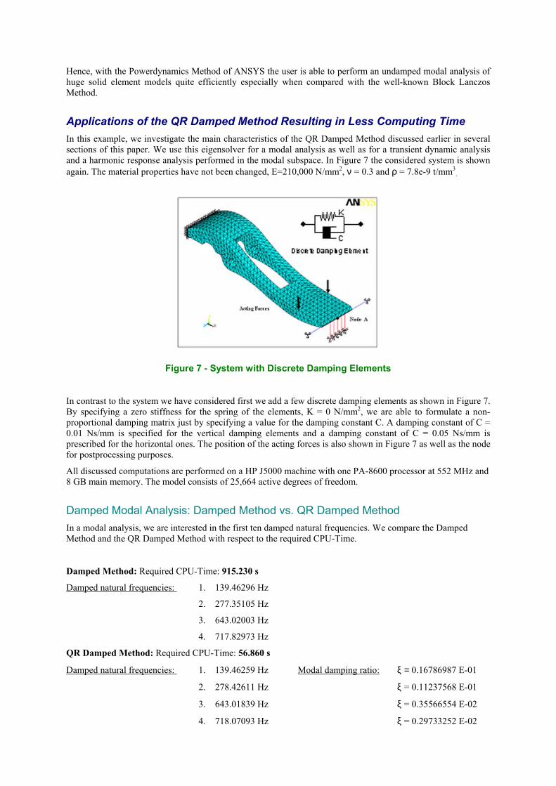
Hence, with the Powerdynamics Method of ANSYS the user is able to perform an undamped modal analysis of huge solid element models quite efficiently especially when compared with the well-known Block Lanczos Method.

Applications of the QR Damped Method Resulting in Less Computing Time In this example, we investigate the main characteristics of the QR Damped Method discussed earlier in several sections of this paper. We use this eigensolver for a modal analysis as well as for a transient dynamic analysis and a harmonic response analysis performed in the modal subspace. In Figure 7 the considered system is shown again. The material properties have not been changed, E=210,000 N/mm2, ν = 0.3 and ρ = 7.8e-9 t/mm3

.

Figure 7 - System with Discrete Damping Elements

In contrast to the system we have considered first we add a few discrete damping elements as shown in Figure 7. By specifying a zero stiffness for the spring of the elements, K = 0 N/mm2, we are able to formulate a non-proportional damping matrix just by specifying a value for the damping constant C. A damping constant of C = 0.01 Ns/mm is specified for the vertical damping elements and a damping constant of C = 0.05 Ns/mm is prescribed for the horizontal ones. The position of the acting forces is also shown in Figure 7 as well as the node for postprocessing purposes.

All discussed computations are performed on a HP J5000 machine with one PA-8600 processor at 552 MHz and 8 GB main memory. The model consists of 25,664 active degrees of freedom.

Damped Modal Analysis: Damped Method vs. QR Damped Method In a modal analysis, we are interested in the first ten damped natural frequencies. We compare the Damped Method and the QR Damped Method with respect to the required CPU-Time.

Damped Method: Required CPU-Time: 915.230 s

Damped natural frequencies: 1. 139.46296 Hz

2. 277.35105 Hz

3. 643.02003 Hz

4. 717.82973 Hz

QR Damped Method: Required CPU-Time: 56.860 s

Damped natural frequencies: 1. 139.46259 Hz Modal damping ratio: ξ = 0.16786987 E-01

2. 278.42611 Hz ξ = 0.11237568 E-01

3. 643.01839 Hz ξ = 0.35566554 E-02

4. 718.07093 Hz ξ = 0.29733252 E-02

In the listing above, we show the results for the first four damped natural frequencies. The results are almost the same but the CPU-Time factor is about 16. Note also, that using the QR Damped Method, the modal damping ratio for each mode is computed.

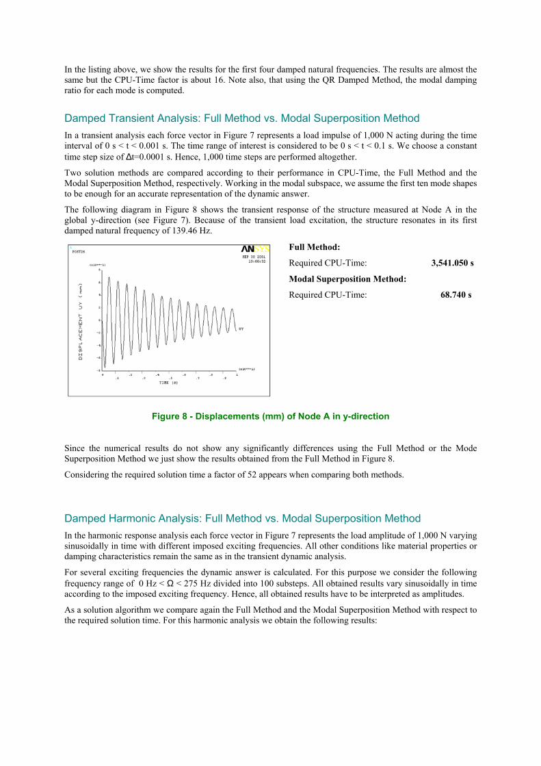
Damped Transient Analysis: Full Method vs. Modal Superposition Method In a transient analysis each force vector in Figure 7 represents a load impulse of 1,000 N acting during the time interval of 0 s < t < 0.001 s. The time range of interest is considered to be 0 s < t < 0.1 s. We choose a constant time step size of ∆t=0.0001 s. Hence, 1,000 time steps are performed altogether.

Two solution methods are compared according to their performance in CPU-Time, the Full Method and the Modal Superposition Method, respectively. Working in the modal subspace, we assume the first ten mode shapes to be enough for an accurate representation of the dynamic answer.

The following diagram in Figure 8 shows the transient response of the structure measured at Node A in the global y-direction (see Figure 7). Because of the transient load excitation, the structure resonates in its first damped natural frequency of 139.46 Hz.

Full Method:

Required CPU-Time: 3,541.050 s

Modal Superposition Method:

Required CPU-Time: 68.740 s

Figure 8 - Displacements (mm) of Node A in y-direction

Since the numerical results do not show any significantly differences using the Full Method or the Mode Superposition Method we just show the results obtained from the Full Method in Figure 8.

Considering the required solution time a factor of 52 appears when comparing both methods.

Damped Harmonic Analysis: Full Method vs. Modal Superposition Method In the harmonic response analysis each force vector in Figure 7 represents the load amplitude of 1,000 N varying sinusoidally in time with different imposed exciting frequencies. All other conditions like material properties or damping characteristics remain the same as in the transient dynamic analysis.

For several exciting frequencies the dynamic answer is calculated. For this purpose we consider the following frequency range of 0 Hz < Ω < 275 Hz divided into 100 substeps. All obtained results vary sinusoidally in time according to the imposed exciting frequency. Hence, all obtained results have to be interpreted as amplitudes.

As a solution algorithm we compare again the Full Method and the Modal Superposition Method with respect to the required solution time. For this harmonic analysis we obtain the following results:

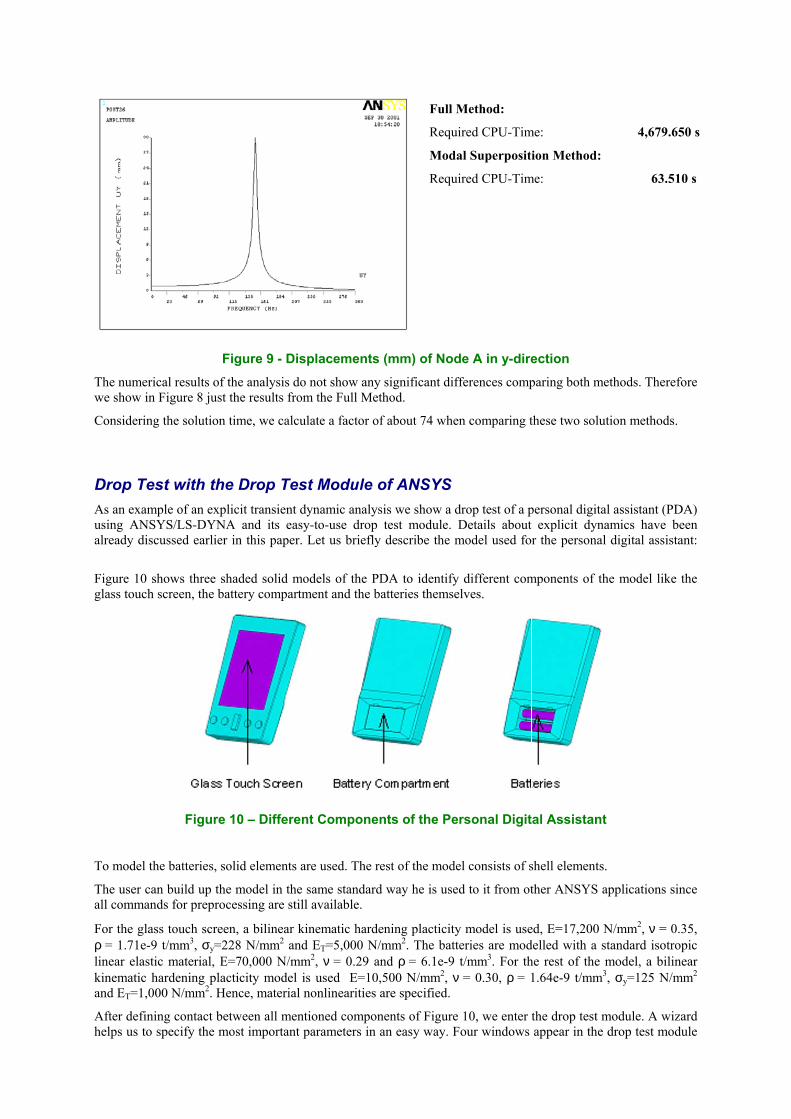
Full Method:

Required CPU-Time: 4,679.650 s

Modal Superposition Method:

Required CPU-Time: 63.510 s

Figure 9 - Displacements (mm) of Node A in y-direction The numerical results of the analysis do not show any significant differences comparing both methods. Therefore we show in Figure 8 just the results from the Full Method.

Considering the solution time, we calculate a factor of about 74 when comparing these two solution methods.

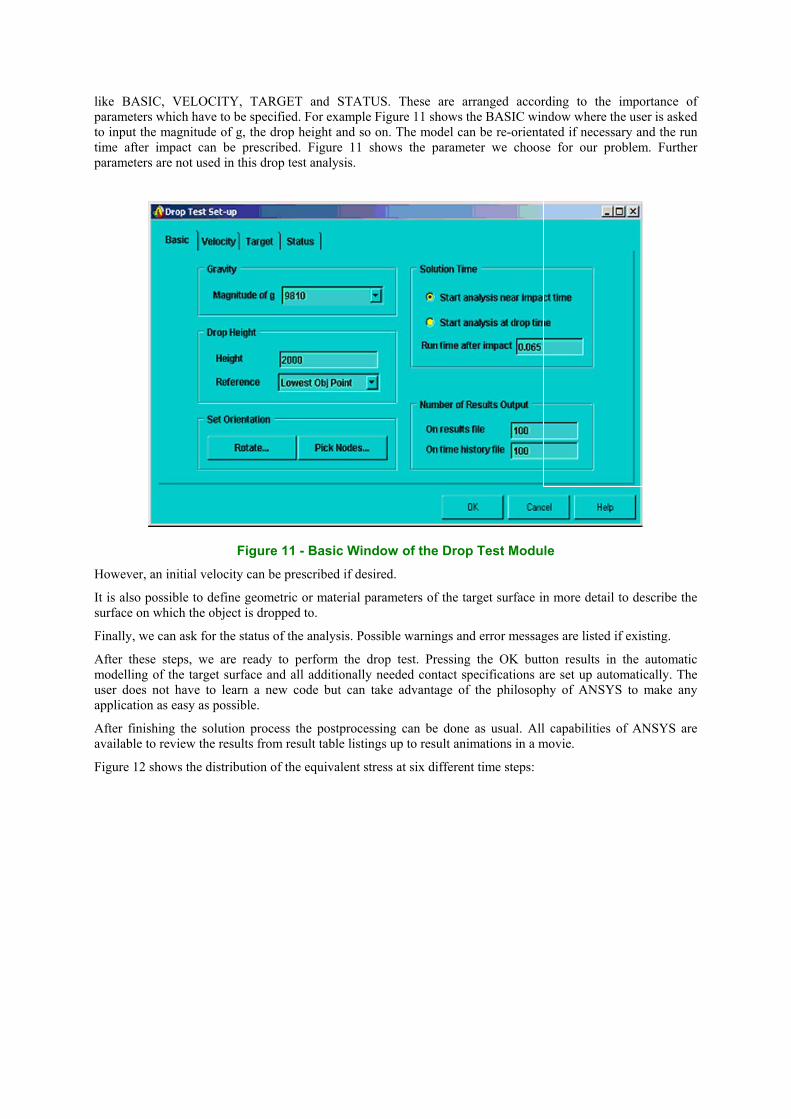
Drop Test with the Drop Test Module of ANSYS As an example of an explicit transient dynamic analysis we show a drop test of a personal digital assistant (PDA) using ANSYS/LS-DYNA and its easy-to-use drop test module. Details about explicit dynamics have been already discussed earlier in this paper. Let us briefly describe the model used for the personal digital assistant:

Figure 10 shows three shaded solid models of the PDA to identify different components of the model like the glass touch screen, the battery compartment and the batteries themselves.

Figure 10 – Different Components of the Personal Digital Assistant

To model the batteries, solid elements are used. The rest of the model consists of shell elements.

The user can build up the model in the same standard way he is used to it from other ANSYS applications since all commands for preprocessing are still available.

For the glass touch screen, a bilinear kinematic hardening placticity model is used, E=17,200 N/mm2, ν = 0.35, ρ = 1.71e-9 t/mm3, σy=228 N/mm2 and ET=5,000 N/mm2. The batteries are modelled with a standard isotropic linear elastic material, E=70,000 N/mm2, ν = 0.29 and ρ = 6.1e-9 t/mm3. For the rest of the model, a bilinear kinematic hardening placticity model is used E=10,500 N/mm2, ν = 0.30, ρ = 1.64e-9 t/mm3, σy=125 N/mm2 and ET=1,000 N/mm2. Hence, material nonlinearities are specified.

After defining contact between all mentioned components of Figure 10, we enter the drop test module. A wizard helps us to specify the most important parameters in an easy way. Four windows appear in the drop test module

like BASIC, VELOCITY, TARGET and STATUS. These are arranged according to the importance of parameters which have to be specified. For example Figure 11 shows the BASIC window where the user is asked to input the magnitude of g, the drop height and so on. The model can be re-orientated if necessary and the run time after impact can be prescribed. Figure 11 shows the parameter we choose for our problem. Further parameters are not used in this drop test analysis.

Figure 11 - Basic Window of the Drop Test Module However, an initial velocity can be prescribed if desired.

It is also possible to define geometric or material parameters of the target surface in more detail to describe the surface on which the object is dropped to.

Finally, we can ask for the status of the analysis. Possible warnings and error messages are listed if existing.

After these steps, we are ready to perform the drop test. Pressing the OK button results in the automatic modelling of the target surface and all additionally needed contact specifications are set up automatically. The user does not have to learn a new code but can take advantage of the philosophy of ANSYS to make any application as easy as possible.

After finishing the solution process the postprocessing can be done as usual. All capabilities of ANSYS are available to review the results from result table listings up to result animations in a movie.

Figure 12 shows the distribution of the equivalent stress at six different time steps:

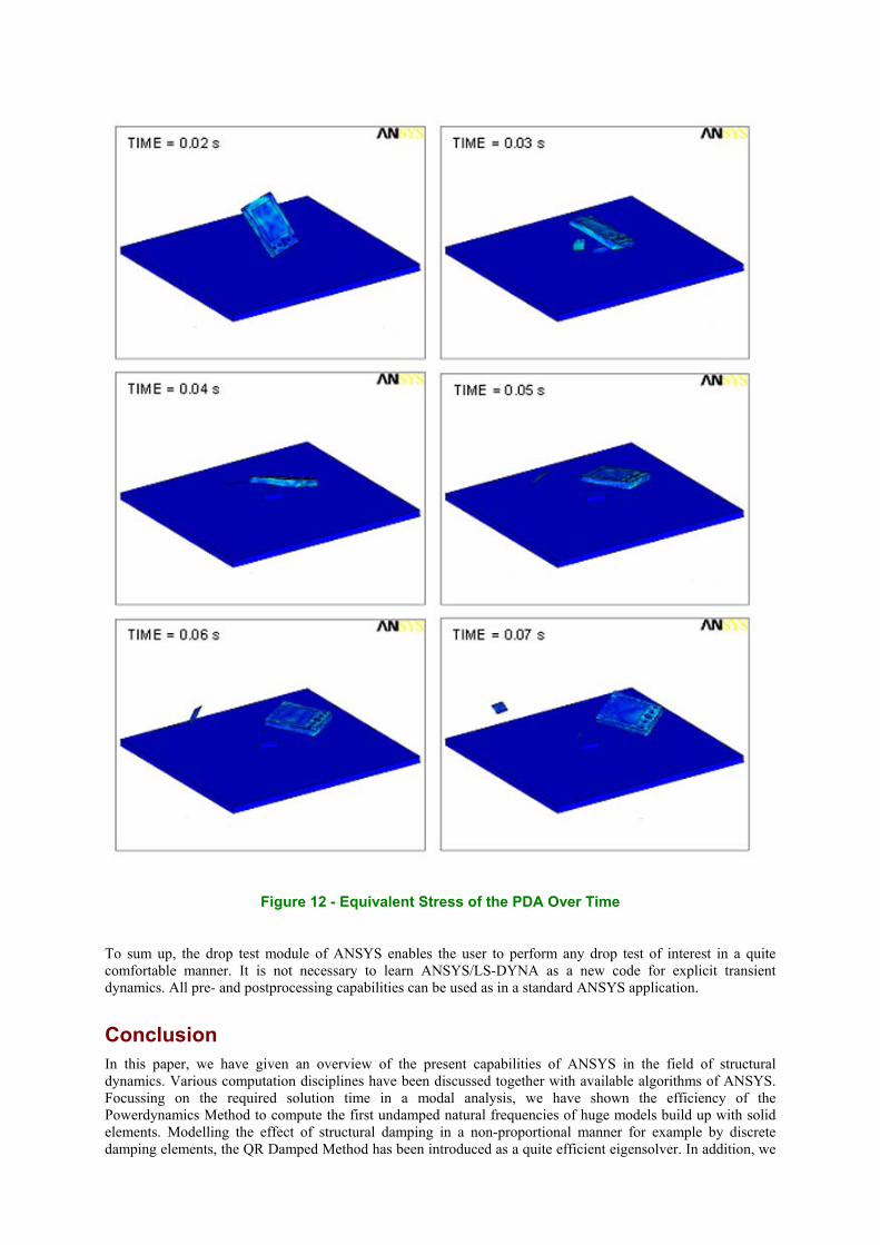
Figure 12 - Equivalent Stress of the PDA Over Time

To sum up, the drop test module of ANSYS enables the user to perform any drop test of interest in a quite comfortable manner. It is not necessary to learn ANSYS/LS-DYNA as a new code for explicit transient dynamics. All pre- and postprocessing capabilities can be used as in a standard ANSYS application.

Conclusion In this paper, we have given an overview of the present capabilities of ANSYS in the field of structural dynamics. Various computation disciplines have been discussed together with available algorithms of ANSYS. Focussing on the required solution time in a modal analysis, we have shown the efficiency of the Powerdynamics Method to compute the first undamped natural frequencies of huge models build up with solid elements. Modelling the effect of structural damping in a non-proportional manner for example by discrete damping elements, the QR Damped Method has been introduced as a quite efficient eigensolver. In addition, we

have mentioned that this algorithm is able to perform a transient, harmonic and also a spectrum analysis quite efficiently in the modal subspace even if non-proportional damping is modelled. Finally, we have demonstrated that the drop test module of ANSYS can solve a typical problem of explicit transient dynamics in a comfortable fashion.

Acknowledgments The authors would like to thank Mr. Steve Pilz and Mr. Tim Pawlak from ANSYS, Inc. who provide very useful material about the ANSYS drop test module. Also special thanks to Dr. Ulrich Stelzmann from CAD-FEM GmbH for many interesting and useful discussions.

References 1) ANSYS/LS-DYNA User’s Guide, Release 5.7, Swanson Analysis Systems, Inc., 2001

2) ANSYS Structural Analysis Guide, Release 5.7, Swanson Analysis Systems, Inc., 2000

3) ANSYS Theory Manual, Release 5.7, Swanson Analysis Systems, Inc., 2001

4) Bathe, K.J., Finite Element Procedures, Prentice-Hall, Englewood Cliffs, New Jersey, 1996

5) Stelzmann, U.: ANSYS Einführungskurs Dynamik, CAD-FEM Seminarunterlagen, 2000

6) Stelzmann, U., Groth, C., Müller, G.: FEM für Praktiker - Band 2: Strukturdynamik, 5. Auflage, expert verlag, 2000