introduction*to*seismic*body*waves*...
TRANSCRIPT

Introduction to seismic body waves Tomography
Presented by Han Zhang
Prepared by group work of Justin Wilgus and Han Zhang

Outlines
1. Velocity derived from wave equation
2. Two commonly used reference 1-‐D models
3. Naming seismic body waves at global scale
4. Basic ideas of body wave tomography
5. Possible improvement on inversion
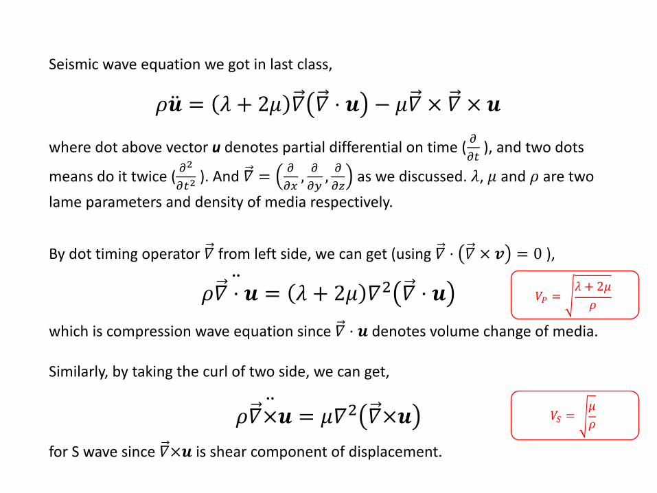
𝜌�̈� = 𝜆 + 2𝜇 𝛻 𝛻 ⋅ 𝒖 − 𝜇𝛻 × 𝛻 × 𝒖
Seismic wave equation we got in last class,
where dot above vector u denotes partial differential on time ( ../
), and two dots
means do it twice ( .0
./0). And 𝛻 = .
.1, ..3, ..4
as we discussed. 𝜆, 𝜇 and 𝜌 are two lame parameters and density of media respectively.
By dot timing operator 𝛻 from left side, we can get (using 𝛻 ⋅ 𝛻 × 𝒗 = 0 ),
𝜌𝛻 ⋅ 𝒖̈ = 𝜆 + 2𝜇 𝛻7 𝛻 ⋅ 𝒖which is compression wave equation since 𝛻 ⋅ 𝒖 denotes volume change of media.
Similarly, by taking the curl of two side, we can get,
𝜌𝛻×𝒖̈ = 𝜇𝛻7 𝛻×𝒖for S wave since 𝛻×𝒖 is shear component of displacement.
𝑉9 =𝜆 + 2𝜇𝜌
�
𝑉; =𝜇𝜌
�
Despite the fact that density of materials inside Earth is increasing with depth, lame parameters 𝜆, 𝜇 are also increasing with depth and their enlargement factor is greater than that of density, which finally leads to an
increase function of wave velocity with depth inside mantle.

Reference Models0
400
800
1200
1600
2000
2400
2800
3200
3600
4000
4400
4800
5200
5600
6000
0 2 4 6 8 10 12 14
220 km
400 km
670 km
CMB
ICB
ρ Vs Vp
Velocity (km/s) or Density (g/cm3)
Dep
th (
km
)
PREM reference model

0
400
800
1200
1600
2000
2400
2800
3200
3600
4000
4400
4800
5200
5600
6000
0 2 4 6 8 10 12 14
410 km
660 km
CMB
ICB
ρ Vs Vp
Velocity (km/s) or Density (g/cm3)
Dep
th (
km
)
AK135 reference model0
400
800
1200
1600
2000
2400
2800
3200
3600
4000
4400
4800
5200
5600
6000
0 2 4 6 8 10 12 14
220 km
400 km
670 km
CMB
ICB
ρ Vs Vp
Velocity (km/s) or Density (g/cm3)
Dep
th (
km
)
PREM reference model0
400
800
1200
1600
2000
2400
2800
3200
3600
4000
4400
4800
5200
5600
6000
0 2 4 6 8 10 12 14
220 km
400 km
670 km
CMB
ICB
ρ Vs Vp
Velocity (km/s) or Density (g/cm3)
Dep
th (
km
)
PREM reference model
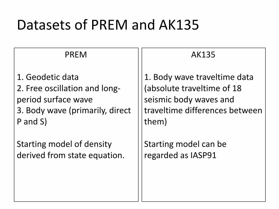
Datasets of PREM and AK135
PREM
1. Geodetic data2. Free oscillation and long-‐period surface wave3. Body wave (primarily, direct P and S)
Starting model of density derived from state equation.
AK135
1. Body wave traveltime data (absolute traveltime of 18 seismic body waves and traveltime differences between them)
Starting model can be regarded as IASP91

Phases Naming (global)
Generally, upgoing waves start with lower case letter while downgoing phases using upper case. Same rule for reflection/conversion points.
Considering difference of sP and SP to see how to name different phases.
source
(Shearer, Intro. to Seismology)

0˚
30˚
60˚
90˚
120˚
150˚
180˚
−150˚
−120˚
−90˚
−60˚
−30˚
Phases Naming (exercise)Blue for P waveRed for S wave
CMB ICB660410
Animation available herehttp://ds.iris.edu/seismon/swaves/index.php
Ray 1 Ray 2
pPcP410s
ScS660ScS

Body Wave TomographyCommon assumptions of body wave traveltime tomography,
1. One good reference model available to make sure velocity perturbation of model region is small enough for linear inversion;
2. All blocks in our model region are well sampled by observations to reduce uncertainty of inversion result.
Idea of body wave traveltime tomography based on ray theory,
1. Traveltime misfit between observed data and prediction of one certain ray is contributed by the blocks lie on this ray path only;
2. Total traveltime perturbation along the ray path can be summed from the product of traveltime in each block (calculated using reference model) with the fractional velocity perturbation within the block.

Body Wave Tomography
1 2 3
4
9
6
7
8
5
For each ray path, we can get one equation looks like this,
𝑟= = ∑ 𝑡=@𝑃@�BCDEFG
where 𝑟= is traveltime misfit between observation and prediction of ray path i, 𝑡=@is absolute traveltime in block j of ray path i, and 𝑃@ is velocity perturbation of block j.
a b c
d fe
g h iFor ray path 1 in the setting showed left, the equation should be,
𝑟H = 𝑃I + 𝑃J + 𝑃Kby assuming 𝑡HI = 𝑡HJ = 𝑡HK = 1 𝑠𝑒𝑐.
𝑟H = 𝑟7 = 𝑟P = 𝑟Q = −0.01 𝑠𝑒𝑐;𝑟S = 𝑟T = 𝑟U = 𝑟V = 𝑟W = 0 𝑠𝑒𝑐;
Rays are numbered aside their arrows and blocks are marked by low-‐case characters inside them. Simple traveltime (1 sec or 2� 𝑠𝑒𝑐 for one block) is assumed for practice.

Body Wave Tomography1 2 3
4
9
6
7
8
5
a b c
d fe
g h i
White blocks have zero perturbation relative to reference model while black ones have perturbation of -‐1%.
𝑟H = 𝑟7 = 𝑟P = 𝑟Q = −0.01 𝑠𝑒𝑐;𝑟S = 𝑟T = 𝑟U = 𝑟V = 𝑟W = 0 𝑠𝑒𝑐;
𝑃I = 𝑃Y = −1%;𝑃B = 𝑃E = 𝑃J = 𝑃[ = 𝑃K = 𝑃\ =𝑃= = 0.

Body Wave TomographyRewrite residual equation using matrix to get general form,
𝒅 = 𝑮𝒎Residuals = Rays × Model
where 𝒅 (1 x i) represents residuals of all the ray path, 𝑮 (j x i) is related to ray path configuration and sensitive kernels adopted and 𝒎 (1 x j) denotes perturbation model.
In the case of i < j, which means the number of independent equations is less than parameters need to be recovered, we can get general solution only (infinitely many solutions).
In the case of i = j, which means we have same amount of independent equations and model parameters, we will get exactly one solution.
In the case of i > j, which means we have more independent equations than model parameters, theoretically we cannot get solution from above form. However, we are able to get least-‐square solution (L2 norm) of this kind of problem by solving
𝑮𝑻𝒅 = 𝑮𝑻𝑮𝒎which theoretically have exactly one solution.

GAP_P4 Model
(Fukao and Obayashi, 2013)
Slab atop at 660 km discontinuity

GAP_P4 Model
(Fukao and Obayashi, 2013)
Slab cross 660 km discontinuity

Possible Improvements
Body wave tomography works pretty well in helping us understand deep Earth structures, however, there are some defects of it, which may be overcame by joint inversion with other dataset. Some are listed here for checking,
1. L2 norm tend to results in a smooth model, which will average small-‐scale heterogeneity to its surroundings. Combining with converted wave modelling (such as receiver function).
2. Limited by the fact that most seismometers are deployed on continents and islands, which leads to poor ray path cover at crust and uppermost mantle beneath ocean. Combing with data from OBSs (ocean bottom seismometers) and/or electrical resistivity tomography (which is also expensive in ocean but is able to get very good shallow structures).


Finite Frequency Kernels
Banana-‐doughnut kernels showing the sensitivity of P-‐wave travel times at 60◦epicentral distance to velocity perturbations in the mantle.
(Hung et al, 2000)