Introduction :Use and misuse of statistics

Garib Murshudov

Not even the most subtle and skilled analysis can overcome completely the unreliability of basic data. Allen, R.G.D. Statistics for Economists

Stolen from “Statistically speaking”

There are three kind of lies: lies, damn lies and (church) statistics

credited to B. Disraeli

__________________________________________________There are thee kind of lies: lies, statistics and Bayesian statistics

Contents

1. Introduction: importance and misuses of statistics2. Use of statistics: two different scenarios3. Introduction to R4. References

IntroductionStatistics is perhaps the most important and at the same time the least appreciated subject in schools

Statistics can (in)validate proposed models. Understanding available tools in statistics may help to improve drawing conclusions and see validity of drawn conclusions.However no statistical treatment can replace good experiment. One has to remember that the results extracted from any sample cannot be better than the sample itself (any data processing reduces information content of the data).

Some misuse of statisticsPsychiatrist: Nearly everybody he meets is neurotic therefore nearly everybody is neurotic.

Problem with the sample

Friends: The number of friends of most of my friends is greater than the number of my friends therefore I am least sociable person.

It is very likely that people who make more friends are my friends also

Averages: Some universities claims about average salary of their graduates. Average can be affected with one extreme outlier

Extrapolations: Mark Twain extrapolates based on observation that:“… In the space of one hundred and seventy-six years the Lower Mississippi

has shortened itself two hundred and forty-two miles. … just a million years ago next November, the Lower Mississippi River was upward of one million

three thousand miles long. …”

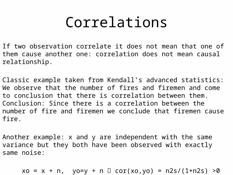
CorrelationsIf two observation correlate it does not mean that one of them cause another one: correlation does not mean causal relationship.

Classic example taken from Kendall’s advanced statistics: We observe that the number of fires and firemen and come to conclusion that there is correlation between them. Conclusion: Since there is a correlation between the number of fire and firemen we conclude that firemen cause fire.

Another example: x and y are independent with the same variance but they both have been observed with exactly same noise:

xo = x + n, yo=y + n cor(xo,yo) = n2s/(1+n2s) >0

n2s is noise to signal ratio.

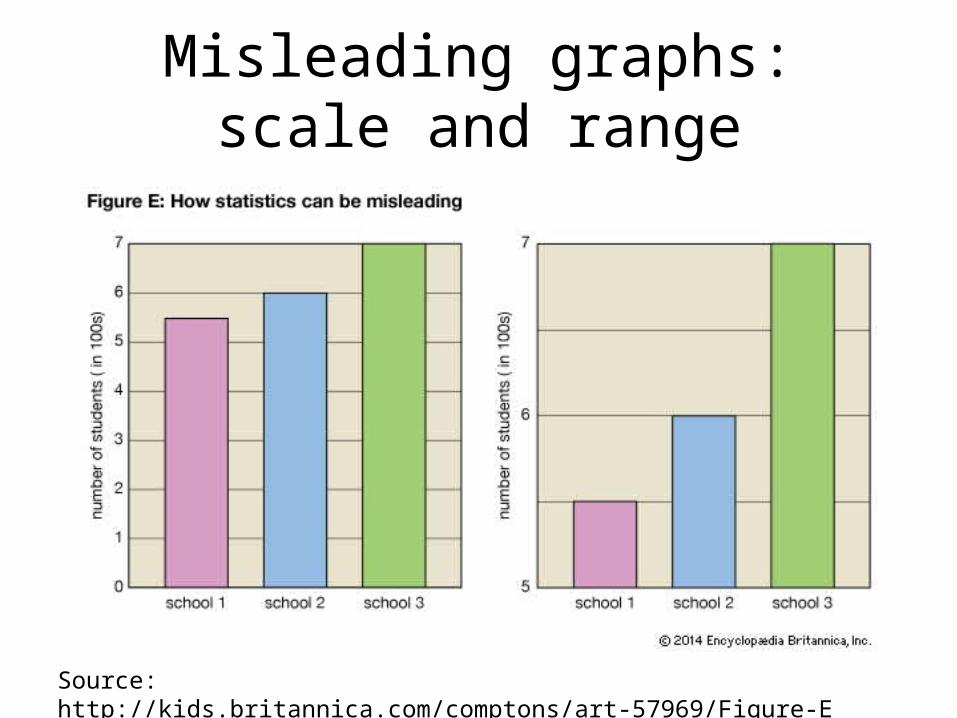
Misleading graphs: scale and range

Source: http://kids.britannica.com/comptons/art-57969/Figure-E

Some uses of statistics:Two different scenarios

Knowledge New system

Model Experiment

EstimateVerify

Predict

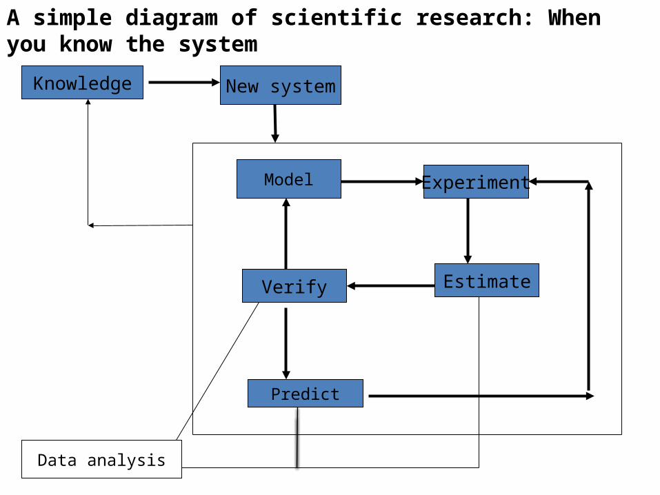
A simple diagram of scientific research: When you know the system

Data analysis

Simple application of Statistics

1. Using previously accumulated knowledge you want to study a system2. Build a model of the system that is based on the previous knowledge3. Set up an experiment and collect data4. Estimate the parameters of the model and change the model if needed5. Verify if parameters are correct and they describe the current model6. Predict the behaviour of the experiment and set up a new experiment. If

prediction gives good results then you have done a good job. If not then you need to reconsider your model and do everything again

7. Once you have done and satisfied then your data as well as model become part of the world knowledge

Data Analysis is used at the stage of estimation, verification and prediction

Simple application of Statistics

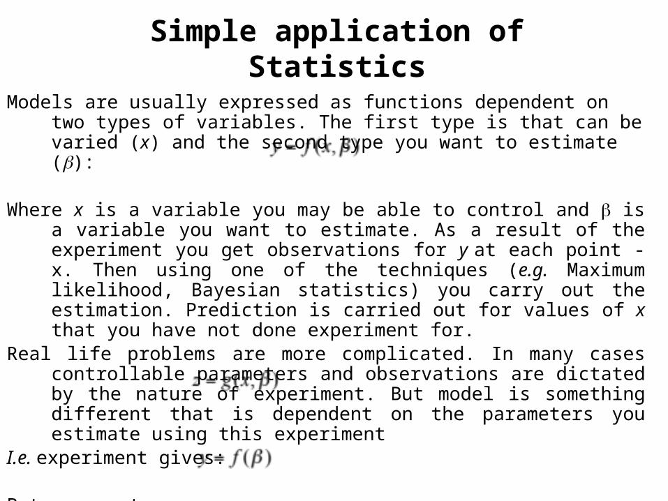
Models are usually expressed as functions dependent on two types of variables. The first type is that can be varied (x) and the second type you want to estimate ():

Where x is a variable you may be able to control and is a variable you want to estimate. As a result of the experiment you get observations for y at each point - x. Then using one of the techniques (e.g. Maximum likelihood, Bayesian statistics) you carry out the estimation. Prediction is carried out for values of x that you have not done experiment for.

Real life problems are more complicated. In many cases controllable parameters and observations are dictated by the nature of experiment. But model is something different that is dependent on the parameters you estimate using this experiment

I.e. experiment gives:

But you want:

Simple application of Statistics

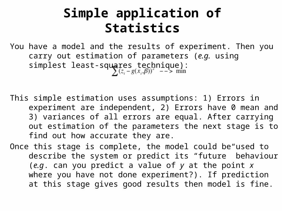
You have a model and the results of experiment. Then you carry out estimation of parameters (e.g. using simplest least-squares technique):

This simple estimation uses assumptions: 1) Errors in experiment are independent, 2) Errors have 0 mean and 3) variances of all errors are equal. After carrying out estimation of the parameters the next stage is to find out how accurate they are.

Once this stage is complete, the model could be used to describe the system or predict its “future” behaviour (e.g. can you predict a value of y at the point x where you have not done experiment?). If prediction at this stage gives good results then model is fine.

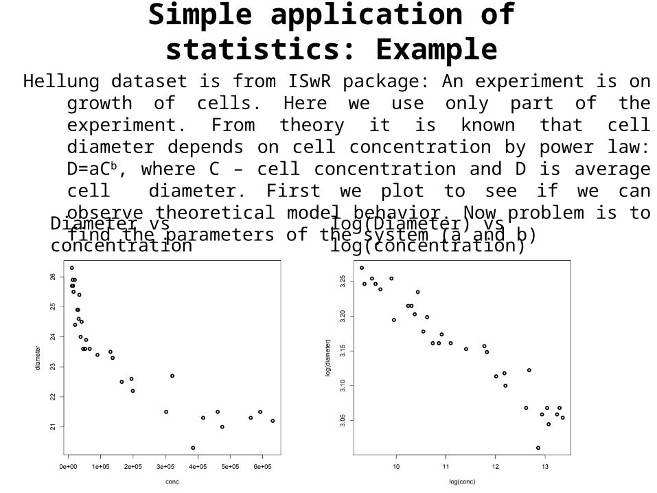
Simple application of statistics: ExampleHellung dataset is from ISwR package: An experiment is on growth of cells. Here we

use only part of the experiment. From theory it is known that cell diameter depends on cell concentration by power law: D=aCb, where C – cell concentration and D is average cell diameter. First we plot to see if we can observe theoretical model behavior. Now problem is to find the parameters of the system (a and b)

Diameter vs concentration log(Diameter) vs log(concentration)

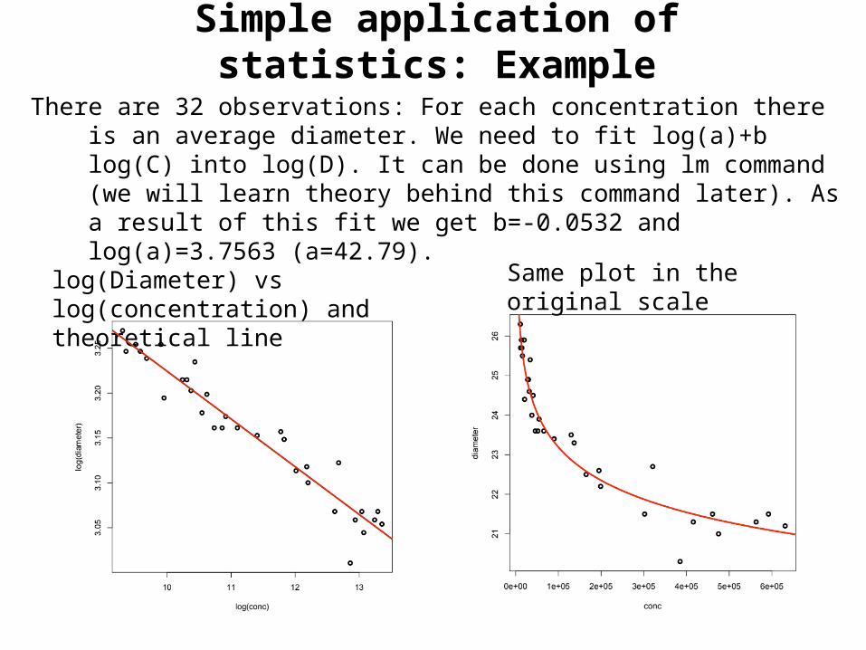
Simple application of statistics: ExampleThere are 32 observations: For each concentration there is an average diameter. We

need to fit log(a)+b log(C) into log(D). It can be done using lm command (we will learn theory behind this command later). As a result of this fit we get b=-0.0532 and log(a)=3.7563 (a=42.79).

log(Diameter) vs log(concentration) and theoretical line

Same plot in the original scale

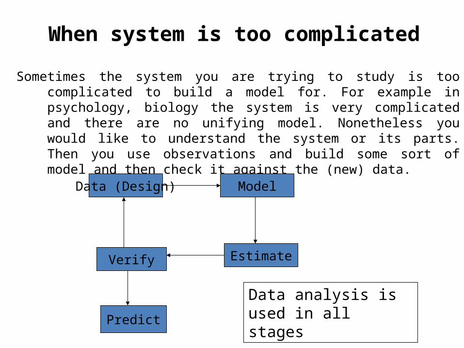
When system is too complicated

Sometimes the system you are trying to study is too complicated to build a model for. For example in psychology, biology the system is very complicated and there are no unifying model. Nonetheless you would like to understand the system or its parts. Then you use observations and build some sort of model and then check it against the (new) data.

Data (Design) Model

EstimateVerify

Predict

Data analysis is used in all stages

When the system is unknown

When you do not know any theoretical model then usually you start from the simplest models: linear models.

If linear model does not fit then start complicating it. By linearity we mean linear on parameters.

This way of modeling could be good if you do not know anything and you want to build a model to understand the system. In later lecture we will learn some of the modeling tools.

When the system is unknown

In many cases simple linear model may not be sufficient. You need to analyse the data before you can build any sort of model.

In these cases you want to find some sort of structure in the data. Even if you can find a structure in the data then it is very good idea to look at the subject where these data came from and try to make sense of it.

Exploratory data analysis techniques might be useful in trying to find a model. Graphical tools such as boxplot, scatter plot, histograms, probability plots, plots of residual after fitting a model into the data etc may give some idea and help to get some sort of sensible model.

We will learn some of the techniques that can give some idea about the structure of the data.

When the system is unknown

When the system is unknown, instead of building the model that can answer to all of your questions you sometimes want to know answer to simple questions. E.g. if effect of two or more factors are significantly different. For example you may want to compare the effects of two different drugs or effects of two different treatments.

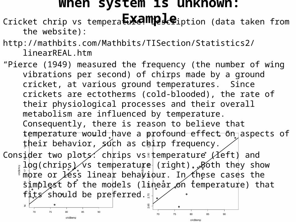
When system is unknown: ExampleCricket chrip vs temperature. Description (data taken from the website):http://mathbits.com/Mathbits/TISection/Statistics2/linearREAL.htm“Pierce (1949) measured the frequency (the number of wing vibrations per second) of

chirps made by a ground cricket, at various ground temperatures.  Since crickets are ectotherms (cold-blooded), the rate of their physiological processes and their overall metabolism are influenced by temperature.  Consequently, there is reason to believe that temperature would have a profound effect on aspects of their behavior, such as chirp frequency.”

Consider two plots: chrips vs temperature (left) and log(chrips) vs temperature (right). Both they show more or less linear behaviour. In these cases the simplest of the models (linear on temperature) that fits should be preferred.

When system is unknown: Various criteria

• Occam’s razor: “entities should not be multiplied beyond necessity” or“All things being equal, the simplest solution tends to be the right one”

A potential problem: There might be conflict between simplicity and accuracy. You can build tree of models that would have different degree of simplicity at different levels

• Rashomon: Multiple choices of models When simplifying a model you may come up up with different simplifications

that have similar prediction errors. In these cases, techniques like bagging (bootstrap aggregation) may be helpful

Introduction to RR is a multipurpose statistical package. It is freely available from:http://www.r-project.org/Or just type R on your google search. The first hit is usually hyperlink to R.

R is an environment (in unix/linux terminology it is some sort of shell) that offers from simple calculation to sophisticated statistical functions.

You can run programs available in R or write your own script using these programs. Or you can also write a program using your favourite language (C,C++,FORTRAN) and add it in R.

If you are a programmer then it is perfect for you. If you are a user it gives you very good options to do what you want to do.

To get started

Useful commands for beginners:help.start()will start a web browser and you can start learning. A very useful section is “An

Introduction to R”. There is a search engine also.To get information about a command, just type?command It will give some sort of help (sometimes helpful). commandgives R script if available. Reading these scripts may help you to write your own

script or program

Simple commands: assignmentThe simplest command is assignmentv=5.0orv <- 5.0the value of the variable v will become 5.0 (Although there are several ways for

assignment I almost always will use =)If you typev = c(1.0,2.0,10.0,1.5,2.5,6.5)will make a vector with length 6.if you typevR will print the value(s) of the variable v.v=c(“mine”,”yours”,”his/hers”,”theirs”,”its”)will create a vector of characters. The type of the variable is defined on fly.To access particular value of a vector use, for examplev[1] – the first element

Simple calculations: arithmetic

All elementary functions are available:exp(v) log(v)tan(v)cos(v) and othersThese functions are applied to all the elements of the vector (or matrix). Types of the

value of these function are the same as the types of the arguments. It will fail if v is a vector of characters and you are trying to use a function that accepts real arguments or the values are outside of the range of function’s argument space.

Apart from elementary functions there are many built in special functions like Bessel functions (besselI(x,n), besselK(x,n) etc), gamma functions and many others. Just have a look help.start() and use “Search engine and Keywords”

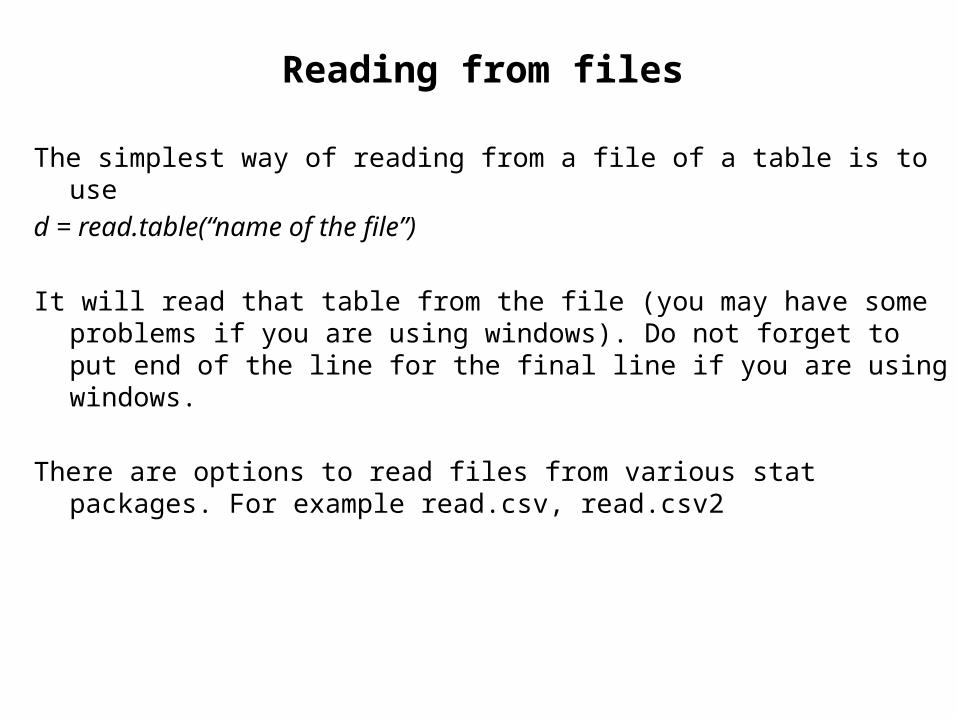
Reading from files

The simplest way of reading from a file of a table is to used = read.table(“name of the file”)

It will read that table from the file (you may have some problems if you are using windows). Do not forget to put end of the line for the final line if you are using windows.

There are options to read files from various stat packages. For example read.csv, read.csv2

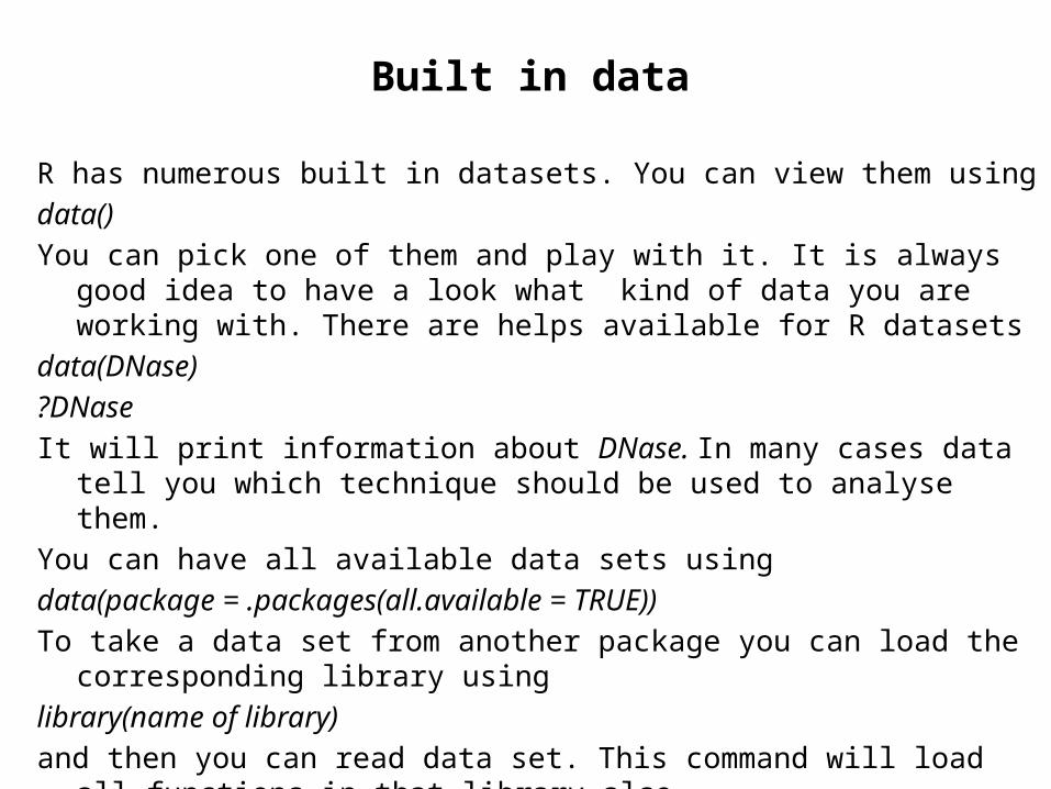
Built in data

R has numerous built in datasets. You can view them usingdata()You can pick one of them and play with it. It is always good idea to have a look what

kind of data you are working with. There are helps available for R datasetsdata(DNase)?DNaseIt will print information about DNase. In many cases data tell you which technique

should be used to analyse them.You can have all available data sets usingdata(package = .packages(all.available = TRUE))To take a data set from another package you can load the corresponding library usinglibrary(name of library)and then you can read data set. This command will load all functions in that library

alsoOnce you have data you can start analyzing them

Installing packages

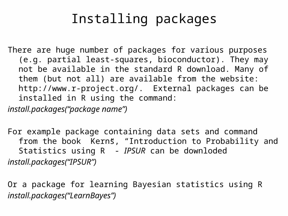
There are huge number of packages for various purposes (e.g. partial least-squares, bioconductor). They may not be available in the standard R download. Many of them (but not all) are available from the website: http://www.r-project.org/. External packages can be installed in R using the command:

install.packages(“package name”)

For example package containing data sets and command from the book Kerns, “Introduction to Probability and Statistics using R” - IPSUR can be downloded

install.packages(“IPSUR”)

Or a package for learning Bayesian statistics using Rinstall.packages(“LearnBayes”)

Simple statistics

The simplest statistics you can calculate are mean, variance and standard deviationsdata(randu) It is a built in data of uniformly distributed random variables. There are three

columns.mean(randu[,2]) # Calculate mean value of the second columnvar(randu[,2])sd(randu[,2])

will calculate mean, variance and standard deviation of the column 2 of the data randu

Another useful command issummary(randu[,2])It gives minimum, 1st quartile, median, mean, 3rd quartile and maximum values

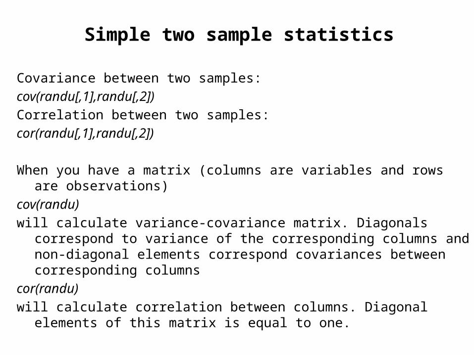
Simple two sample statistics

Covariance between two samples:cov(randu[,1],randu[,2])Correlation between two samples:cor(randu[,1],randu[,2])

When you have a matrix (columns are variables and rows are observations)cov(randu)will calculate variance-covariance matrix. Diagonals correspond to variance of the

corresponding columns and non-diagonal elements correspond covariances between corresponding columns

cor(randu) will calculate correlation between columns. Diagonal elements of this matrix is equal

to one.

Simple plots

There are several useful plot functions. We will learn some of them during the course. Here are the simplest ones:

plot(randu[,2])Plots values vs indices. The x axis is index of the data points and the y axis is its

value

Simple plots: boxplotAnother useful plot is boxplot.require(MASS)boxplot(shoes)It produces a boxplot. It is a useful plot that may show extreme outliers and overall

behaviour of the data under consideration. It plots median, 1st, 3rd quantiles, minimum and maximum values. In some sense it a graphical representation of command summary. It also plots several boxplots alongside if the argument is the list of vectors.

Simple plots: histogram

Description: Histogram is a tabulated frequencies and usually displayed as bars. The range of datapoints is divided into bins and the number of datapoints falling into each bin is calculated. If bin size is equal then midpoints of bins vs the number of points in this bins is plotted (If the empirical density of a probability distribution is desired then the number of points in each bin is divided by the total number).

There are various ways of calculating the number of bins. Two most popular ones are: Sturges where bin size is equal to range(sample)/(1+log2n), where range is the difference between maximum and minimum and 2) Scott’s method where bin size is 3.5σ/n1/3, where σ is the sample standard deviation. Often Scott’s method gives visually better histograms. By default R’s hist command uses Sturges method

Histogram is a useful tool to visually inspect location, skewness, presence of outliers, multiple modes.

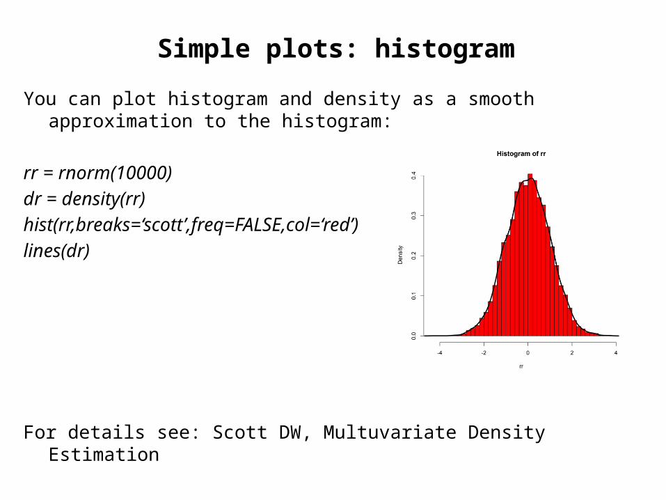
Simple plots: histogram

You can plot histogram and density as a smooth approximation to the histogram:

rr = rnorm(10000)dr = density(rr)hist(rr,breaks=‘scott’,freq=FALSE,col=‘red’)lines(dr)

For details see: Scott DW, Multuvariate Density Estimation

Simple plots: qqplot

Description: qqplot is a qunatile-quantile plot. It is used for graphical comparison of the distributions of two random variables. It can be used to compare two samples or one sample against a theoretical distribution. Quantile is a fraction of points below a given number. For example if 0.25 (25%) of all data are below x25 then this point is called 0.25 (25%) quantlile. 0.25 quantile is also called first quartile, 0.5 quantile is median.

For two given samples, quantiles are calculated and then they are plotted against each other. If the resulting plot is linear it means that one random variable can be derived from another using a linear transformation.

If you have two cumulative probability distribution (empirical or theoretical) – F and G then QQ plot is plot of x and y related as:

F(y) = G(x) y = F-1(G(x))

Simple plots: qqplot

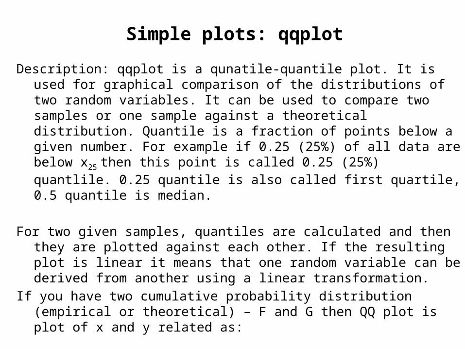
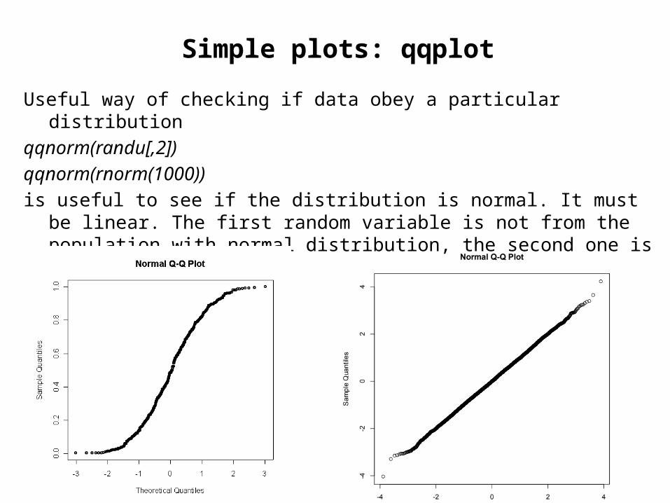
Useful way of checking if data obey a particular distributionqqnorm(randu[,2])qqnorm(rnorm(1000))is useful to see if the distribution is normal. It must be linear. The first random

variable is not from the population with normal distribution, the second one is

Simple qqplot

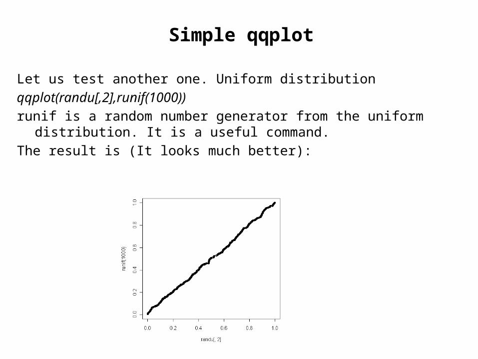
Let us test another one. Uniform distributionqqplot(randu[,2],runif(1000))runif is a random number generator from the uniform distribution. It is a useful

command. The result is (It looks much better):

Further reading

1) “Introduction to R” from package R2) Dalgaard, P “Introductory statistics with R”3) Kerns, JC. “Introduction to Probability and Statistics using R”4) Scott DW, Multivariate Density Estimation5) Huff, D, “How to lie with Statistics”6) Gaither, CC and Cavazoz-Gaither, AE “Statistically Speaking:

dictionary of quotations”