introduction to symplectic topology by dusa mcdu & …jchaidez/solutions/salamonmcduff.pdf ·...

Introduction To Symplectic Topology

By Dusa Mcduff & Dietmar Salamon

Solutions By Julian C. Chaidez

Exercise 1.5 Carry out the inverse Legendre transform from a Hamiltonian system to a Lagrangian

system.

Solution 1.5 Suppose that we are given a Hamiltonian H with det( ∂H∂yi∂yj

) 6= 0. Then we define:

vk =∂H

∂yk; L(t, x, v) =

∑k

ykvk −H(t, x, v)

Now we show that if γ(t) = (x(t), y(t)) satisfies Hamiltons equations for H, then (x, dxdt

) satisfy the Euler-

Lagrange equations for L. First we see that due to Hamilton’s equations, we have:

dxkdt

=∂H

∂yk= vk;

dykdt

= −∂H∂xk

We observe that:

d

dt(∂L

∂vk) =

d

dt(∂

∂vk(∑j

yjvj −H(t, x, v))) =d

dt(yk −

∂H

∂vk+∑j

∂yj∂vk

vj)

Then we see: ∑j

vj∂yj∂vk

=∑j

dxjdt

∂yj∂vk

=∑j

∂H

∂yj

∂yj∂vk

=∂H

∂vk

Thus:d

dt(∂L

∂vk) =

dykdt

= −∂H∂xk

Furthermore we have:

∂L

∂xk=

∂

∂xk(∑j

yj∂H

∂vj−H(t, x, v)) = −∂H

∂xk+∑j

∂yj∂xk

vj + yj∂vj∂xk− ∂H

∂vj

∂vj∂xk

= −∂H∂xk

Here the equality of the last two terms comes from the fact that∂yj∂xk

= 0 and yj = ∂H∂vj

. This proves the

result

Exercise 1.12 Show that the set Symp(R2n) of symplectomorphisms of R2n form a group.

Solution 1.12 The identity map Id : R2n is a smooth symplectomorphism since its Jacobian is the

identity map TR2n → TR2n, which is evidently symplectic. Furthermore given φ, ψ ∈ Symp(R2n) we can

compose them to get a diffeomorphism ψ φ and since d(ψ φ) = dψ dφ, the fact that dψ and dφ are

symplectic and that symplectic matrices are a group implies that d(ψφ) is symplectic. Finally, the inverse

1

diffeomorphism φ−1 has d(φ−1) = (dφ)−1, thus its Jacobian is also in the linear symplectic group, so it is

a symplectomorphism. Associativity follows from the same property for group composition in Diff. Thus

concludes the proof.

Exercise 1.13 Consider the matrix:

Φ =

(A B

C D

)where A.B,C and D are real n× n matrices. Prove that Φ is symplectic if and only if its inverse is of the

form

Φ−1 =

(DT −BT

−CT AT

)Deduce that a 2× 2 matrix is symplectic if and only if its determinant is equal to 1.

Solution 1.13 We simply carry out the matrix multiplication. Φ is symplectic if and only if:

ΦTJΦ =

(AT CT

BT DT

)(0 −1

1 0

)(A B

C D

)=

(AT CT

BT DT

)(−C −DA B

)=

(CTA− ATC CTB − ATDDTA−BTC DTB −BTD

)=

(0 −1

1 0

)Furthermore we see that the inverse condition is true if and only if:(

DT −BT

−CT AT

)(A B

C D

)=

(DTA−BTC DTB −BTD

ATC − CTA ATD − CTB

)=

(1 0

0 1

)From these expressions it is evident that these two conditions are equivalent, since they are both true if

and only if CTA − ATC = DTB − BTD = 0 and DTA − BTC = ATD − CTB = 1. In the n = 1 case,

this is equivalent to ad− bc = 1 (i.e the determinant 1 condition). The other condition is trivially satisfied

since 1× 1 matrix commute.

Exercise 1.15 Find an element of the linear group SL(4,R) which is not in Sp(4,R).

Solution 1.15 One cheap way of doing this is to just find a linear φ where φ∗ω = −ω. Then:

φ∗(ω2) = φ∗ω ∧ φ∗ω = (−1)2ω2 = ω2

Such a map φ is given, for example, by the matrix 4× 4:

Φ =

(1 0

0 −1

)

Exercise 1.17 (Confirming Lemma 1.17) The Poisson bracket satisfies the Jacobi identity.

2

Solution 1.17 We will write this out in Einstein index notation, which will make it clear where the signs

are coming from, then we will switch to a more invariant notation. Let J = (jab) be the co-symplectic

matrix/form in coordinates. Furthermore let f, g, h ∈ C∞(R2n). Then:

f, g, h = ∂cfjcd∂d(∂agj

ab∂bh) = ∂chjcd∂d∂agj

ab∂bh+ ∂chjcd∂agj

ab∂d∂bh

= ∂chjcd∂d∂agj

ab∂bh− ∂chjcd∂agjba∂d∂bh = d2g(Jdf, Jdh)− d2h(Jdf, Jdg)

It is clear that if we sum over the cyclic permutations of f, g and h, the result will vanish due to term

matching.

Exercise 1.19 How does the Poisson bracket behave with respect to product of functions? Prove that

the Poisson bracket of two functions f and g is given by:

f, g = ω0(Xf , Xg)

Solution 1.19 The Poisson bracket obeys a Leibniz rule. We see that:

fg, h = −(∇(fg))TJ0∇h = f(−(∇g)TJ0∇h) + g(−(∇f)TJ0∇h) = fg, h+ gf, h

We can use the fact that fg, h = h, fg to show the analogous identity for the other entry.

For the second part, we just observe that:

−(∇f)TJ0∇g = −(∇f)T (−J0)J0(−J0)∇g = (−J0∇f)TJ0(−J0∇g) = ω0(Xf , Xg)

Exercise 1.20 Check that in the Kepler problem (Example 1.7) the three components of the angular

momentum x× x are integrals of motion which are not in involution.

Solution 1.20 In the Kepler problem we have p = dxdt

. To show that the elements of x× p = x× dxdt

are

invariants of motion we just have to show that ddt

(x× dxdt

) = 0. But:

d

dt(x× dx

dt) =

dx

dt× dx

dt+ x× dx2

dt= x× −x

|x|2= 0

Now observe that the whole system is symmetric under orthogonal transformations (in fact this is where

these conserved quantities come from, via Noether’s theorem). Thus to check that these integrals of motion

are not in involution, we need only check it for one pair of components. Take f(x, p) = (x×p)1 = x2p3−x3p2

3

and g(x, p) = (x× p)2 = x3p1 − x1p3. Then we just see that:

∇f =

0

p3

−p2

0

−x3

x2

;∇g =

−p3

0

p1

x3

0

−x1

Thus it is easy to calculate f, g = −(∇g)J0∇f = x2p1− x2p1 (there may be a sign error here but this is

irrelevant for showing that it’s not 0).

Exercise 1.22 Consider the Hamiltonian:

H =n∑j=1

aj(x2j + y2

j )

with aj > 0. Find the solution of the corresponding Hamiltonian differential equation. Prove that this

system is integrable. Find all periodic solutions on the energy surface H = c for c > 0.

Solution 1.22 Consider Hi(x, y) = x2i + y2

i . In the coordinates (x1, y1, . . . , xn, yn) the matrix J0 splits

into blocks where on the (xi, yi) each block acts as the standard 90 degree rotation. Thus we evidently have

ω0(dHi, dHj) = 0. Thus any linear combination H =∑

i aiHi has the property that the Hi are conserved

quantities, due to the linearity of the Poisson bracket. Thus the system is integrable.

If we examine the defining ODE for the Hamiltonian flow, we see that:

(dxidt,dyidt

) = −ai(−yi, xi)

Therefore the integral curves of the Hamiltonian system are precisely the vectors:

(xi(t), yi(t)) = (ri cos(−ait), ri sin(−ait))

Here r2 =∑

i r2i .

Now I ⊂ 1, . . . , n. Then we make the following claim: an orbit (ri cos(−ait), ri sin(−ait)) with ri > 0

if and only if i ∈ I is periodic if and only if there exists an s such that ais2π∈ Z for all i ∈ I. If this is the

case, then evidently any such orbit is s-periodic. Conversely, if such an orbit (ri cos(−ait), ri sin(−ait)) is

s-periodic, then ais ∈ 2πZ for all i ∈ I.

To see that the system is integrable, we show that we can find n conserved quantities Hi with Hi, Hj =

0 and H,Hi = 0 for all i, j. We take:

Hi =1

2(x2

i + y2i )

4

so that ∂Hi∂xj

= δijxi and ∂Hi∂yj

= δijyi. Then:

Hi, Hj =∑k

∂Hi

∂xk

∂Hj

∂yk− ∂Hi

∂yk

∂Hj

∂xk=∑k

xiyjδikδjk − yixjδikδjk

The above expression is 0 if i 6= j since then either δik = 0 or δjk = 0. If i = j, then the expression

is 0 because F, F = −F, F and thus F, F = 0 for any function F . Thus these are n commuting

conserved quantities which commute with H since H =∑

i aiHi and the Poisson bracket is bilinear.

Exercise 1.23 Carry out the Legendre transformation for the geodesic flow. Prove that the g-norm of

the velocity |x|g =√〈x, g(x)x〉 is constant along every geodesic.

Solution 1.23 We have that the conjugate momentum is pi = gijyj and thus that yj = gijpi. Therefore

under the Legendre transform we have:

H(x, p) = piyi − L(x, y) = gijpipj −1

2gijy

iyj = gijpipj −1

2gijpipj =

1

2gijpipj

Hamilton’s equations are:dxidt

=dH

dqi= gijpi

dpkdt

=−1

2

∂gij

∂xkpipj

We see that:

|dxidt|2 = gij

dxidt

dxjdt

= gijgikgjlqkql = gijqiqj = 2H(x, p)

So the g-norm is conserved.

Exercise 1.24 (Exponential Map) Assume g(x) = 1 for large x so that the solutions x(t) of Equation

(1.12) exist for all time. The solution with initial conditions x(0) = x and x(0) = ξ is called the geodesic

through (x, ξ). Define the exponential map:

E : Rn × Rn → Rn, E(x, ξ) = x(1)

where x(t) is the geodesic through (x, ξ). Prove that this geodesic is given by x(t) = E(x, tξ). Prove that

there exists a constant c > 0 such that:

|E(x, ξ)− x− ξ| ≤ c|ξ|2

and deduce that:∂Ej∂xk

(x, 0) =∂Ej∂ξk

(x, 0) = δij,∂2Ej∂xk∂ξl

(x, 0) = 0

5

Solution 1.24 Given a point p and velocity ξ, let x(t) be the geodesic defined for t ∈ [0,∞) with x(0) = p

and dxdt

(0) = ξ. Then observe that xr(t) = x(rt) satisfies:

d2xirdt2

(t) = r2d2xi

dt2(rt) = r2Γijk(x(rt))

dxj

dt(rt)

dxk

dt(rt) = Γijk(x(rt))

dxj(rt)

dt

dxk(rt)

dt

Thus xr is a geodesic with initial velocity rξ and initial point p, and it follows from uniqueness of ODE

solutions that this is the unique solution. It thus follows that x(t) = xt(1) = E(p, tξ).

To show the estimate, note that the geodesic equations yield:

| dxdt2| ≤ C|dx

dt|2 ≤ C|ξ|2

Here C = supx∈Rn(|Γijk|) (which exists because g ≡ 1 outside of a compact set) and we use the fact that

|dxdt|2 is conserved. Also we may assume that the norm is just the typical Euclidean norm when writing the

estimate, since on any compact set K there exists a ck with |v|2g ≤ CK |v|2 where |v| is the usual Euclidean

norm. Again, we may use the “compact support” of g to conclude that we can pick a constant so that

such an inequality holds for all x ∈ Rn.

Thus we may write:

|dxdt

(t)− dx

dt(0)| ≤

∫ 1

0

| dxdt2| ≤ C|ξ|2t

|x(1)− x(0)− dx

dt(0)| ≤ |

∫ 1

0

dx

dt(t)− dx

dt(0)| ≤

∫ 1

0

|dxdt

(t)− dx

dt(0)| ≤ C|ξ|2

This is precisely our estimate.

This estimate implies the derivative identities, as it gives us the Taylor expansion:

Ek(x, ξ) = xk + ξk + |ξ|2hk(x, ξ)

Thus we have:∂Ek

∂xj= δkj +O(ξ)

∂Ek

∂ξj= δkj +O(ξ)

∂Ek

∂xi∂ξj= 0 + 2ξj

∂h

∂xi+ |ξ|2 ∂h

∂xi∂ξj

Exercise 1.25 Suppose that φ : Rn → Rn is a diffeomorphism and:

g(x) = φ∗h(x) = dφ(x)Th(φ(x))dφ(x)

Prove that every geodesic x(t) for g is mapped under φ to a geodesic y(t) = φ(x(t)) for h. Deduce that

the concept of the exponential map extends to manifolds.

6

Solution 1.25 We calculate using Einstein notation. The geodesic equations for the metric h = φ∗g and

a curve x are:

gkl∂mφk∂jφ

ldxj

dt+

1

2(∂i(gkl∂mφ

k∂jφl) + ∂j(gkl∂mφ

k∂iφl)− ∂m(gkl∂iφ

k∂jφl))dxi

dt

dxj

dt

= gkl∂mφk∂jφ

ldxj

dt+

1

2(∂iφ

n∂ngkl∂mφk∂jφ

l+gkl∂i∂mφk∂jφ

l+gkl∂mφk∂i∂jφ

l+∂jφn∂ngkl∂mφ

k∂iφl+gkl∂j∂mφ

k

+gkl∂mφk∂j∂iφ

l − ∂mφn∂ngkl∂iφk∂jφl − gkl∂m∂iφk∂j∂l − gkl∂iφk∂m∂jφl)dxi

dt

dxj

dt

= gkl∂mφk∂jφ

ldxj

dt+ gkl∂mφ

k∂i∂jφldx

i

dt

dxj

dt

+1

2(∂ngkl∂iφ

n∂mφk∂jφ

l + ∂ngkl∂jφn∂mφ

k∂iφl − ∂ngkl∂mφn∂iφk∂jφl)

dxi

dt

dxj

dt

From the second to third line we cancel some terms in the 12(. . . ) part and reorganize the rest of the terms

into two pieces. On the other hand the geodesic equations for the metrix g and the curve φ(x) is:

gmkd

dt2(φ(x)j) +

1

2(∂kglm + ∂lgkm − ∂mgkl)∂iφk

dxi

dt∂jφ

ldxj

dt

= gmk(∂i∂jφk dx

i

dt

dxj

dt+ ∂iφ

k dxi

dt2) +

1

2(∂kglm + ∂lgkm − ∂mgkl)∂iφk

dxi

dt∂jφ

ldxj

dt

These two systems of equations for x merely differ by composition with the Jacobian (∂φ) on the m index

of the latter equation. Thus the second system vanishes if and only if the first does. This shows that

geodesics are coordinate independent.

Exercise 1.26 The covariant derivative of a vector field ξ(s) ∈ Rn along a curve x(s) ∈ Rn is defined by:

(∇ξ)k = ξk +n∑

i,j=1

Γkijxξj

A submanifold L ⊂ Rn is called totally geodesic if ∇x(s) ∈ Tx(s)L for every smooth curve x(s) ∈ L. Prove

taht L is totally geodesic if and only if TL is invariant under the geodesic flow.

Solution 1.26 First suppose that L were closed under geodesic flow. Pick a p ∈ L and pass to coordinates

U about p where p is 0 and L ∩ U ' Rk ∩ U ⊂ U ⊂ Rn. Then any geodesic x with x(0) = p = 0 anddxdt

(0) = ξ has:

dxk

dt2|p = −(

n∑i,j=1

Γkijdxi

dt

dxj

dt)|p = η

Now suppose that the the left term were not in TLp. Then for small time ε we have dxdt

(ε) = tη + O(t2)

and thus x(ε) = 0 + εξ + ε2

2η + O(ε3) (in coordinates). Now we may split η into η = ηL + ηL⊥ , a parallel

7

and non-parallel component. Then we may write:

x(ε) = εξ +ε2

2η|| +

ε2

2η⊥ +O(ε3) = v||(ε) +

1

2ε2η⊥ +O(ε3)

Taking ε → 0 we see that the result must have some non-zero perpendicular component to x(ε). Thus it

must be the case that η ∈ TLp, and thus that −(∑n

i,j=1 Γkijξiξj)|p ∈ TLp for any p ∈ L. This implies that

∇(dxdt

(s)) ∈ Tx(s)L since dxdt

(s) is parallel to L for any such curve.

Conversely, suppose that L is not closed under geodesic flow. Then there exists a geodesic x with

x(0) = p ∈ L and dxdt

(0) ∈ TLp, but x(t) 6∈ L for some t.

Exercise 2.1 Let (V, ω) be a symplectic vector space and Φ : V → V be a linear map. Prove that Φ is

a linear symplecticmorphism if and only if its graph

ΓΦ = (v,Φv) ∈ V ⊕ V |v ∈ V

is Lagrangian in V ⊕ V with symplectic form ω = (−ω)⊕ ω.

Solution 2.1 If Φ is Lagrangian then for any v ∈ V we have:

ω(v ⊕ Φv, w ⊕ Φw) = −ω(v, w) + ω(Φv,Φw) = Φ∗ω(v, w)− ω(v, w)

Thus Φ∗ω(v, w) = ω(v, w) for all v, w ∈ V if and only if ΓΦ is Lagrangrian.

Exercise 2.9 Identify a matrix with its graph as in Exercise 2.1 and use a construction similar to that

in Exercise 2.8 to interpret the composition of symplectic matrices in terms of symplectic reduction.

Solution 2.9 Let (Vi, ωi), i = 1, 2, 3, be three symplectic vector spaces with φ12 : V1 → V2 and φ23 : V2 →V3 with graphs Γ12 ⊂ V1⊕V2, Γ23 ⊂ V2⊕V3. Then consider the symplectic vector space V1⊕V2⊕V2⊕V3 with

symplectic form (−ω1)⊕ω2⊕(−ω2)⊕ω3. Furthermore consider the subspaces Γ12⊕Γ23 and W = V1⊕∆⊕V3.

The first subspace is Lagrangian and the second is coisotropic with symplectic perpendicular W ω =

0⊕∆⊕0. We can see that this is equal to the symplectic perpendicular because it has dimension 4n−3n = n

and is contained in the symplectic perpendicular by direct computation. Under symplectic reduction we

have the identification W/W ω = V1 ⊕ V3 with symplectic form (−ω1)⊕ ω3. Furthermore:

(Γ12 ⊕ Γ23) ∩W = v1 ⊕ φ12(v1)⊕ v2 ⊕ φ23(v2)|φ1(v1) = v2

and thus under the quotient the Lagrangian Γ12 ⊕ Γ23 goes to the Lagrangian:

Γ13 = v1 ⊕ v2|v2 = φ23(φ12(v1))

Thus we can interpret composition of symplectomorphisms in terms of taking a product of their graphs

and then performing a symplectic reduction along W .

8

Exercise 2.10 Let (V, ω) be a symplectic vector space and W ⊂ V be any subspace. Prove that the

quotient V ′ = W/(W ∩W ω) carries a natural symplectic structure.

Solution 2.10 We simply define the symplectic form ω([v], [w]) := ω(v, w). To show that this is well-

defined, suppose that v′ = v+ a and w′ = w+ b with a, b ∈ W ∩W ω. Then ω(v′, w′) = ω(v, w) +ω(a, w) +

ω(v, b) + ω(a, b) = ω(v, w). To show that ω is non-degenerate, suppose that we see that ω([v], [w]) = 0 for

some [v] and all [w]. Then ω(v, w) = 0 for v ∈ W and all w ∈ W , so v ∈ W ω ∩W and thus [v] = [0]. This

proves non-degeneracy. Bilinearity and anti-symmetry follow from the definition.

Exercise 2.11 Let A = −AT ∈ R2nn be a non-degenerate skew-symmetric matrix and define ω(z, w) =

〈Az,w〉. Prove that a symplectic basis for (R2n, ω) can be constructed from the eigenvectors uj + ivj of A.

Solution 2.11 Consider the matrix iA. This matrix is Hermitian, thus it admits a diagonalization with

eigenvectors xi = ui+ ivi and real eigenvalues λi. This is also a diagonalization of A with eigenvalues −iλi.Since A is non-degenerate, λi 6= 0 for any i. Now observe that iA(ui + ivi) = −Avi + iAui = λiui + iλivi.

Since A is real, it preserves real and imaginary vectors, so it follows that Avi = −λiui and Aui = λivi. This

implies that A(ui − ivi) = −λi(ui − ivi). Thus eigenspaces occur in conjugate pairs, and the eigenvectors

are of the form ±λ1, . . . ,±λn.

Now let ei = 1|ui|ui and fi = −1

λi|ui|vi (here we take only the λi > 0). Then we have:

ω(ei, fi) = 〈ei, Afi〉 = 〈ei, ei〉 = 1

Thus the subspace ei, fi is symplectic. Furthermore, we can choose the ui+ ivi so that u1± iv1, . . . , un± ivnis orthonormal. Since each span span(ei, fi) = span(ui, vi) is a union of the ±λi eigenspaces, and since

eigenspaces of a self-adjoint operator are perpendicular, it follows that the spans span(ei, fi) are mutually

symplectic orthogonal. Thus e1, f1, . . . , en, fn is a symplectic basis.

Exercise 2.12 Consider a smooth family of symplectic forms ωt(z, w) = 〈z, Atw〉 on R2n. Prove Corollary

2.4 by considering the family of subspaces Et ⊂ C2n generated by the eignevectors of At corresponding to

the eigenvalues with positive imaginary part.

Solution 2.12 This is a less general version of Exercise 2.61. See that exercise: the proof is essentially

the same, except here it is over I instead of a general simply connected neighborhood U ⊂ Rn.

Exercise 2.13 Show that if β is any skew-symmetric bilinear form on the vector space W , there is a

basis u1, . . . , un, v1, . . . , vn of W such that β(uj, vk) = δjk and all other pairings β(b1, b2) vanish.

Solution 2.13 Let φ : W → W ∗ be the map v 7→ β(v, ·) and let B = ker(φ). Let b1, . . . , bk and take any

complimentary subspace V ⊂ W so that W = V ⊕B. Then β|V is non-degenerate on V since β(u, v) = 0

9

for some u ∈ V and all v ∈ V implies that β(u, v + b) = 0 for all v ∈ V and b ∈ B as well, thus that

u ∈ B ∩ V = 0. Thus we can find a symplectic basis e1, f1, . . . , en, fn on V by Theorem 2.3.

Exercise 2.14 Show that if W is an isotropic, coisotropic or symplectic subspace of (V, ω) then any

standard basis for (W,ω) extends to a symplectic basis for (V, ω).

Solution 2.14 If W is symplectic, then we can take a symplectic basis e1, f1, . . . , ek, fk and a symplectic

basis ek+1, fk+1, . . . , en, fn of W ω. The union of the bases is then a symplectic basis of V , since pairings of

a basis element from W with those of W ω are necessarily 0.

Now let W be isotropic. We prove that we can extend any basis to a symplectic basis of V inductively. If

W is 1-dimensional, this is trivial. Now suppose W is k > 1 dimensional and let b1, . . . , bk be a basis. Then

W ′ = span(b1, . . . , bk−1) is an isotropic subspace and by the induction assumption we may extend its basis

to a symplectic basis a1, b1, . . . , ak−1, bk−1, e1, f1, . . . , en−k−1, fn−k−1. Let U = span(a1, b1, . . . , ak−1, bk−1)

and observe that Uω = span(e1, f1, . . . , en−k−1, fn−k−1). Now observe that there must exist an ei or fisuch that ω(ei, bk) 6= 0 (resp. ω(fi, bk) 6= 0). Otherwise bk ∈ U ∩ span(b1, . . . , bk−1)ω = span(b1, . . . , bk−1),

contradicting that bi is a basis. Thus we may rescale the ei or fi to an ak so that ω(ak, bk) = 1. Then the

resulting a1, b1, . . . , ak, bk is a symplectic basis of its span, and we extend this to a symplectic basis of V .

Then given a standard basis of W , e1, f1, . . . , en, fn, b1, . . . , bk and let U = span(e1, f1, . . . , en, fn). Then

b1, . . . , bk spans an isotropic subspace of the symplectic space Uω, so we may use the previous result to

find an extension of b1, . . . , bk to a symplectic basis of Uω, and then combine the bases to get an extension

e1, f1, . . . , en, fn, a1, b1, . . . , ak, bk.

Exercise 2.15 Show that any hyperplane W in a 2n-dimensional symplectic vectorspace is coisotropic.

Thus W ω ⊂ W and ω|W has rank 2(n− 1).

Solution 2.15 Simply observe that any 1-dimensional subspace is isotropic. Indeed, ω(v, v) = 0 for

any v. Then any hyperplane H has Hω 1-dimensional, and thus isotropic. Then since the symplectic

perpendicular to an isotropic space is coisotropic, we have (Hω)ω = H is coisotropic.

Exercise 2.16 Let Ω(V ) denote the space of all symplectic forms on the vector space V . By considering

the action of GL(2n,R) on Ω(V ) given by ω 7→ Φ∗ω show that Ω(V ) ' GL(2n,R)/Sp(2n).

Solution 2.16 By Theorem 2.3 we know that the action of GL(2n,R) is transitive. Furthermore, the

stabilizer of any symplectic form is isomorphic to the symplectic group. In fact, if ω = Φ∗ω0 then:

Stab(ω) = Φ−1SΦ|S ∈ Sp(2n) = Φ−1Sp(2n)Φ

Thus the map GL(2n,R)/Sp(2n)→ Ω(V ) given by:

[Φ] 7→ Φ∗ω0

10

is bijective and smooth with respect to the smooth structure on the homogeneous space GL(2n,R)/Sp(2n).

Note that to prove the smoothness of this map really rigorously we need to know a slice theorem for Lie

group actions, which we will not develop here.

Exercise 2.17 (The Gelfand-Robbin quotient) It has been noted by physicists for a long time that

symplectic structures often arise from boundary value problems. The underlying abstract principle can be

formulated as follows. Let H be a Hilbert space and D : dom(D) → H be a symmetric linear operator

with a closed graph and a dense domain dom(D) ⊂ H. Prove that the quotient:

V = dom(D∗)/dom(D)

is a symplectic vector space with symplectic structure:

ω([x], [y]) = 〈x,D∗y〉 − 〈D∗x, y〉

Solution 2.17 First we prove that ω is well-defined and symplectic. First suppose that [x′] = [x] so that

x′ = x+ a, a ∈ dom(D). Then:

ω([x′], [y]) = 〈x,D∗y〉+ 〈a,D∗y〉 − 〈D∗x, y〉 − 〈D∗a, y〉 = 〈x,D∗y〉 − 〈D∗a, y〉+ 〈D∗(a− a), y〉

= 〈x,D∗y〉 − 〈D∗x, y〉 = ω([x], [y])

And similarly ω([x], [y′]) = ω([x], [y]) if [y′] = [y]. The form is anti-symmetric by construction. To show

that it is non-degenerate, suppose that ω([x], [y]) = 0 for all [y] and some [x]. Then:

〈x,D∗y〉 − 〈D∗x, y〉 = 0

for all y ∈ dom(D∗) and x ∈ dom(D∗).

To see that Λ0 is a Lagrangian subspace, first observe for any x, y ∈ Λ0 we have D∗x = D∗y = 0, thus

ω([x], [y]) = 0. Thus Λ0 ⊂ Λω0 . Similarly, if y ∈ Λω

0 , then 〈D∗x, y〉 − 〈x,D∗y〉 = 〈x,D∗y〉 = 0 for every

x ∈ Λ0.

Exercise 2.18 Consider the linear operator:

D = J0d

dtJ0 =

(0 −1

1 0

)on the Hilbert space H = L2([0, 1],R2n) with dom(D) = W 1,2

0 ([0, 1],R2n). Show that in this case the

Gelfand-Robbin quotient is given by V = R2n × R2n with symplectic form (−ω0)× ω0.

11

Solution 2.18 The definition of dom(D∗) is all of the y ∈ H such that the map x 7→ 〈y,Dx〉 extends

from dom(D) to H. This is the map:

x 7→∫ 1

0

〈y, J0dx

dt〉dt

Now observe that if this map extends to H then y is differentiable in the weak sense, thus in W 1,2 ⊂L2. Furthermore the Sobolev inequalities imply that W 1,2 functions are continuous in dimension 1, and

continuity implies absolute continuity on a compact domain. Thus dom(D∗) ⊂ W 1,2([0, 1],R2n), the

Sobolev space with no boundary limitations. Furthermore, for any y ∈ W 1,2([0, 1],R2n) and any x ∈dom(D) we have: ∫ 1

0

〈y, J0dx

dt〉dt =

∫ 1

0

−〈J0dy

dt, x〉dt

There is no boundary contribution due to the vanishing of x at the ends of [0, 1]. Thus W 1,2([0, 1],R2n) ⊂dom(D∗) and they are therefore equal.

Continuing, we may characterize dom(D∗)/dom(D) as R2n⊕R2n. Indeed, we have [x] = [x′] if and only

if we have x − x′ ∈ W 1,20 ([0, 1],R2n), i.e if and only if x(0) = x′(0) and x(1) = x′(1) (the other conditions

are automatically satisfied). The map to the quotient can thus be given by x 7→ (x(0), y(0)) ∈ R2n ⊕ R2n.

Then if we consider [x], [y] ∈ V = dom(D∗)/dom(D), we see that:

ω([x], [y]) =

∫ 1

0

〈J0dy

dt, x〉 − 〈J0

dx

dt, y〉dt =

∫d

dt〈J0y, x〉dt = 〈J0y(1), x(1)〉 − 〈J0y(0), x(0)〉

This is precisely the symplectci from ω0 ⊕−ω0.

Exercise 2.24 (i) Show that if Φ ∈ Sp(2n) is diagonalizable, then it can be diagonalized with a symplectic

matrix. (ii) Deduce from Lemma 2.20 that the eigenvalues of Φ ∈ Sp(2n) occur either in pairs λ, λ−1 ∈ R,

λ, λ ∈ S1, or in complex quadruplets λ, λ−1, λ, λ−1. (iii) Work out the conjugacy classes for matrices in

Sp(2) and Sp(4).

Solution 2.24 (i) Let Φ ∈ Sp(2n) be diagonalizable by GL(2n,R). Let e1, . . . , e2n be a basis of eigen-

vectors. Then ω(ei, ej) = ω(Φei,Φej) = λiλjω(ei, ej), so either ω(ei, ej) = 0 or λiλj = 1 for any pair ei, ejof eigenvectors. In particular, let Vλ = spanei|Φei = λ±1

i ei. Then V ωλ = ⊕λ′∈σ(Φ)|λ′ 6=λVλ′ (here by σ(Φ)

we denote the set of eigenvalues with |λ| ≥ 1 so that we don’t double count). To see this, observe that we

have ⊕λ′∈σ(Φ)|λ′ 6=λVλ′ ⊂ V ωλ and by dimension counting they must be equal. Thus ω|Vλ is symplectic, and

Φ splits as a direct sum of symplectic maps Φ = Φλ ⊕ Φωλ with Φλ : Vλ → Vλ and Φω

λ : V ωλ → V ω

λ .

The above discussion implies that V splits symplectically as V = ⊕λ∈σ(Φ)Vλ with Φ splitting as

⊕λ∈σ(Φ)Φλ. Each Φλ has only two eigenvalues, λ±1, or only 1 is λ = ±1. By the symplectic Graham-

Schmidt procedure, we know that we can find a symplectic basis ei, fi such that for every i we have

ei, fi ∈ Vλ for some λ and so that the collection of ei, fi with this property form a symplectic basis for Vλ.

Thus we can get Φ into the block form ⊕λΦλ via a symplectic transformation and it suffices to show that

we may find a symplectic change of basis on each Vλ individually to get Φλ into diagonal form.

Thus we may assume that we are in one of two cases. In the first case, Φ : V → V has two real

12

eigenvalues, λ and λ−1. In the second case, λ has only one eigenvalue, ±1. In the second case, Φ = ±Iand is already diagonalized. Thus we may restrict to the first case.

Therefore assume that Φ : V → V is a symplectomorphism with only two eigenvalues, λ and λ−1 with

|λ| > 1. Thus V = Vλ ⊕ Vλ−1 . Now let e ∈ Vλ. Since Vλ ⊂ eω we must be able to pick an f ∈ Vλ−1

so that ω(e, f) = 1 by non-degeneracy. Now consider W = span(e, f). Then Vλ ∩ fω ⊂ eω ∩ fω = W ω

and likewise eω ∩ Vλ−1 ⊂ eω ∩ fω = W ω. We have dim(Vλ ∩ fω) = dim(Vλ) − 1 since fω is codimension

1 in V and it does not contain Vλ since e ∈ Vλ, and likewise dim(eω ∩ Vλ−1) = dim(Vλ−1) − 1. Thus

W ω = (Vλ ∩ fω)⊕ (Vλ−1 ∩ eω). We see that for any w = u+ v ∈ W ω with u ∈ Vλ ∩ fω and v ∈ Vλ−1 ∩ eω,

then Φw = λu + λ−1v ∈ W ω. Thus we may recurse our argument onto V ′ = W ω, and by repeating it

acquire a symplectic basis e1, . . . , ek, f1, . . . , fk where Φei = λei and Φfi = λ−1fi. This concludes the proof.

(ii) By Lemma 2.20, for a symplectic matrix S, λ ∈ σ(S) implies that λ−1 ∈ σ(S). Furthermore

λ ∈ σ(S) implies λ ∈ σ(S) because S is real. Thus we have 3 cases. If λ is real, then λ = λ λ occurs in a

pair λ, λ−1. If λ is complex and unit norm, then λ = λ−1 so λ occurs in a pair λ, λ ∈ U(1). If λ is both

complex and non-unit length, then λ, λ, λ−1, λ−1 are all distinct. So λ occurs in that group of 4.

(iii) Here we will use the fact that if two real matrices M,N are similar over GL(n,C) if and only if

they are similar over GL(n,R).

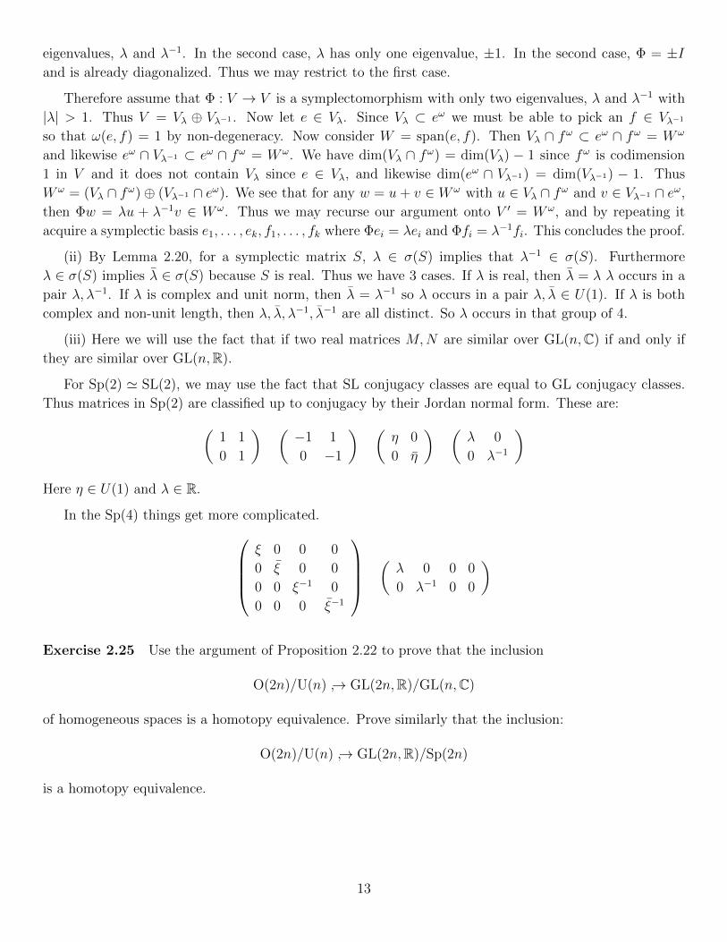
For Sp(2) ' SL(2), we may use the fact that SL conjugacy classes are equal to GL conjugacy classes.

Thus matrices in Sp(2) are classified up to conjugacy by their Jordan normal form. These are:(1 1

0 1

) (−1 1

0 −1

) (η 0

0 η

) (λ 0

0 λ−1

)Here η ∈ U(1) and λ ∈ R.

In the Sp(4) things get more complicated.ξ 0 0 0

0 ξ 0 0

0 0 ξ−1 0

0 0 0 ξ−1

(λ 0 0 0

0 λ−1 0 0

)

Exercise 2.25 Use the argument of Proposition 2.22 to prove that the inclusion

O(2n)/U(n) → GL(2n,R)/GL(n,C)

of homogeneous spaces is a homotopy equivalence. Prove similarly that the inclusion:

O(2n)/U(n) → GL(2n,R)/Sp(2n)

is a homotopy equivalence.

13

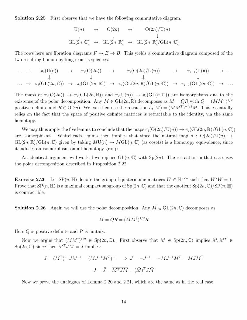
Solution 2.25 First observe that we have the following commutative diagram.

U(n) → O(2n) → O(2n)/U(n)

↓ ↓ ↓GL(2n,C) → GL(2n,R) → GL(2n,R)/GL(n,C)

The rows here are fibration diagrams F → E → B. This yields a commutative diagram composed of the

two resulting homotopy long exact sequences.

. . . → πi(U(n)) → πi(O(2n)) → πi(O(2n)/U(n)) → πi−1(U(n)) → . . .

↓ ↓ ↓ ↓. . . → πi(GL(2n,C)) → πi(GL(2n,R)) → πi(GL(2n,R)/GL(n,C)) → πi−1(GL(2n,C)) → . . .

The maps of πi(O(2n)) → πi(GL(2n,R)) and πi(U(n)) → πi(GL(n,C)) are isomorphisms due to the

existence of the polar decomposition. Any M ∈ GL(2n,R) decomposes as M = QR with Q = (MMT )1/2

positive definite and R ∈ O(2n). We can then use the retraction ht(M) = (MMT )−t/2M . This essentially

relies on the fact that the space of positive definite matrices is retractable to the identity, via the same

homotopy.

We may thus apply the five lemma to conclude that the maps πi(O(2n)/U(n))→ πi(GL(2n,R)/GL(n,C))

are isomorphisms. Whiteheads lemma then implies that since the natural map q : O(2n)/U(n) →GL(2n,R)/GL(n,C) given by taking MU(n) → MGL(n,C) (as cosets) is a homotopy equivalence, since

it induces an isomorphism on all homotopy groups.

An identical argument will work if we replace GL(n,C) with Sp(2n). The retraction in that case uses

the polar decomposition described in Proposition 2.22.

Exercise 2.26 Let SP(n,H) denote the group of quaternionic matrices W ∈ Hn×n such that W ∗W = 1.

Prove that SP(n,H) is a maximal compact subgroup of Sp(2n,C) and that the quotient Sp(2n,C)/SP(n,H)

is contractible.

Solution 2.26 Again we will use the polar decomposition. Any M ∈ GL(2n,C) decomposes as:

M = QR = (MM †)1/2R

Here Q is positive definite and R is unitary.

Now we argue that (MM †)1/2 ∈ Sp(2n,C). First observe that M ∈ Sp(2n,C) implies M,MT ∈Sp(2n,C) since then MTJM = J implies:

J = (MT )−1JM−1 = (MJ−1MT )−1 =⇒ J = −J−1 = −MJ−1MT = MJMT

J = J = MTJM = (M)TJM

Now we prove the analogues of Lemma 2.20 and 2.21, which are the same as in the real case.

14

We have MT = JM−1J−1 so MT is conjugate to M−1 and thus they have the same eigenvalues.

Therefore M and M−1 have the same eigenvalues, and thus if λ ∈ σ(M) has λ 6= ±1 then λ−1 ∈ σ(M).

Since det(M) = 1, we must therefore have an even number of −1 eigenvalues and since dim(M) = 2n, we

have an even number of the remaining 1 eigenvalues as well.

Now observe that if if v and w are in eigenspaces of M with eigenvalues λ, λ′ and λ′ 6= λ−1 then they

are symplectic orthogonal. Indeed:

ω(v, w) = ω(Mv,Mw) = λλ′ω(v, w)

So if λλ′ 6= 1 then ω(v, w) = 0. Then we can argue again that if P = P † and P ∈ Sp(2n,C) then

Pα ∈ Sp(2n,C) for all α ∈ R. We can check this by splitting C2n into eigenspaces. If v, w in non-

complimentary eigenspaces then ω(Pαv, P αw) = ω(v, w) = 0 and otherwise:

ω(Pαv, Pαw) = (λλ−1)αω(v, w) = ω(v, w)

Thus (MM †)−α/2 ∈ Sp(2n,C) for α ∈ [0, 1] and thus the homotopy ht(M) = (MM †)−α/2M is a

retraction of Sp(2n,C) to U(n) ∩ Sp(2n,C).

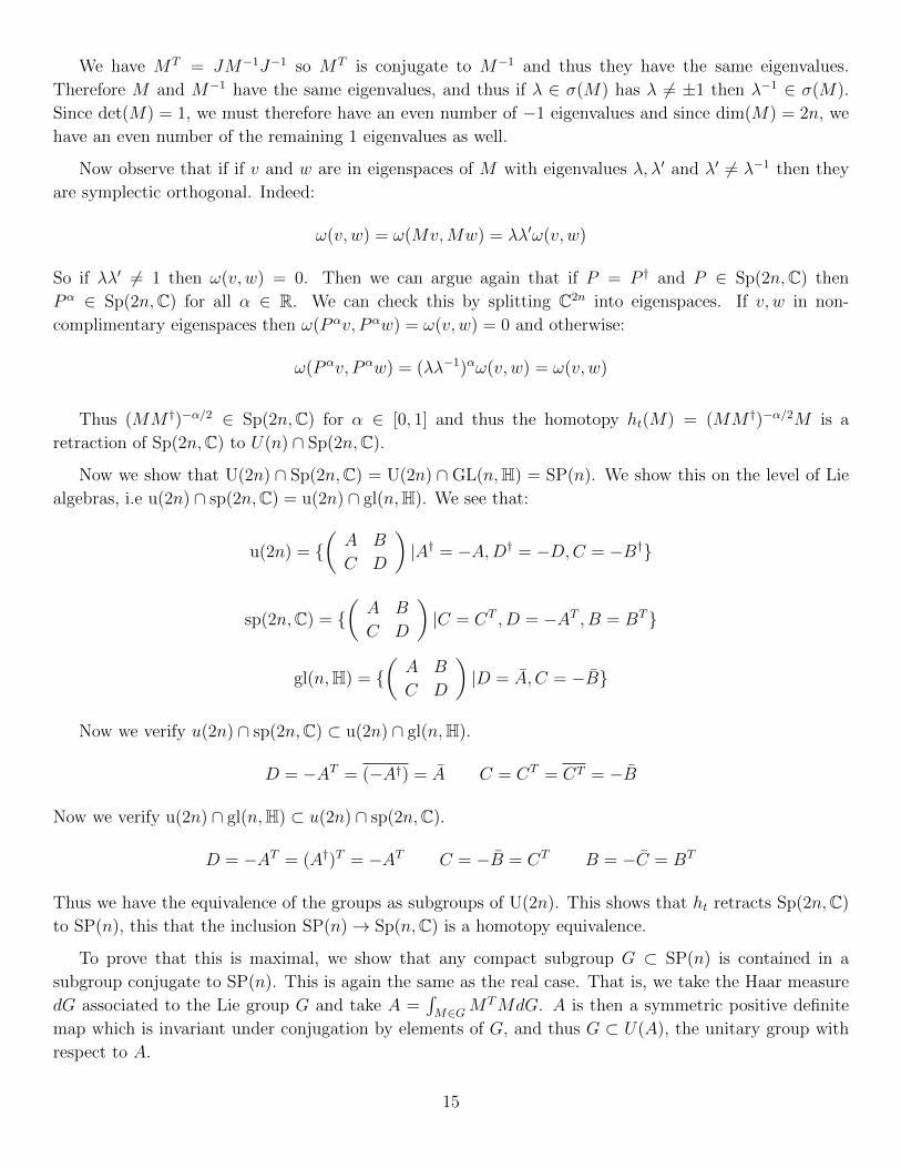
Now we show that U(2n) ∩ Sp(2n,C) = U(2n) ∩ GL(n,H) = SP(n). We show this on the level of Lie

algebras, i.e u(2n) ∩ sp(2n,C) = u(2n) ∩ gl(n,H). We see that:

u(2n) = (A B

C D

)|A† = −A,D† = −D,C = −B†

sp(2n,C) = (A B

C D

)|C = CT , D = −AT , B = BT

gl(n,H) = (A B

C D

)|D = A, C = −B

Now we verify u(2n) ∩ sp(2n,C) ⊂ u(2n) ∩ gl(n,H).

D = −AT = (−A†) = A C = CT = CT = −B

Now we verify u(2n) ∩ gl(n,H) ⊂ u(2n) ∩ sp(2n,C).

D = −AT = (A†)T = −AT C = −B = CT B = −C = BT

Thus we have the equivalence of the groups as subgroups of U(2n). This shows that ht retracts Sp(2n,C)

to SP(n), this that the inclusion SP(n)→ Sp(n,C) is a homotopy equivalence.

To prove that this is maximal, we show that any compact subgroup G ⊂ SP(n) is contained in a

subgroup conjugate to SP(n). This is again the same as the real case. That is, we take the Haar measure

dG associated to the Lie group G and take A =∫M∈GM

TMdG. A is then a symmetric positive definite

map which is invariant under conjugation by elements of G, and thus G ⊂ U(A), the unitary group with

respect to A.

15

Furthermore A is symplectic. This is a poorly elaborated point in the book! We see this as so:

ATJA =

∫M×N∈G×G

M †MJN †NdGdG

=

∫M×M∈∆⊂G×G

M †MJM †MdG+

∫M×N∈M×N−∆

1

2(MTMJNTN +NTNJMTM)dGdG

= J

∫M×M∈∆⊂G×G

dG+

∫M×N∈M×N−∆

1

2(MTMJNTN −MTMJNTN)dGdG = J

Thus we may use the conjugation map G → U(2n) given by M 7→ A−1/2MA1/2 to see that it is

conjugate to a subgroup of SP)(n).

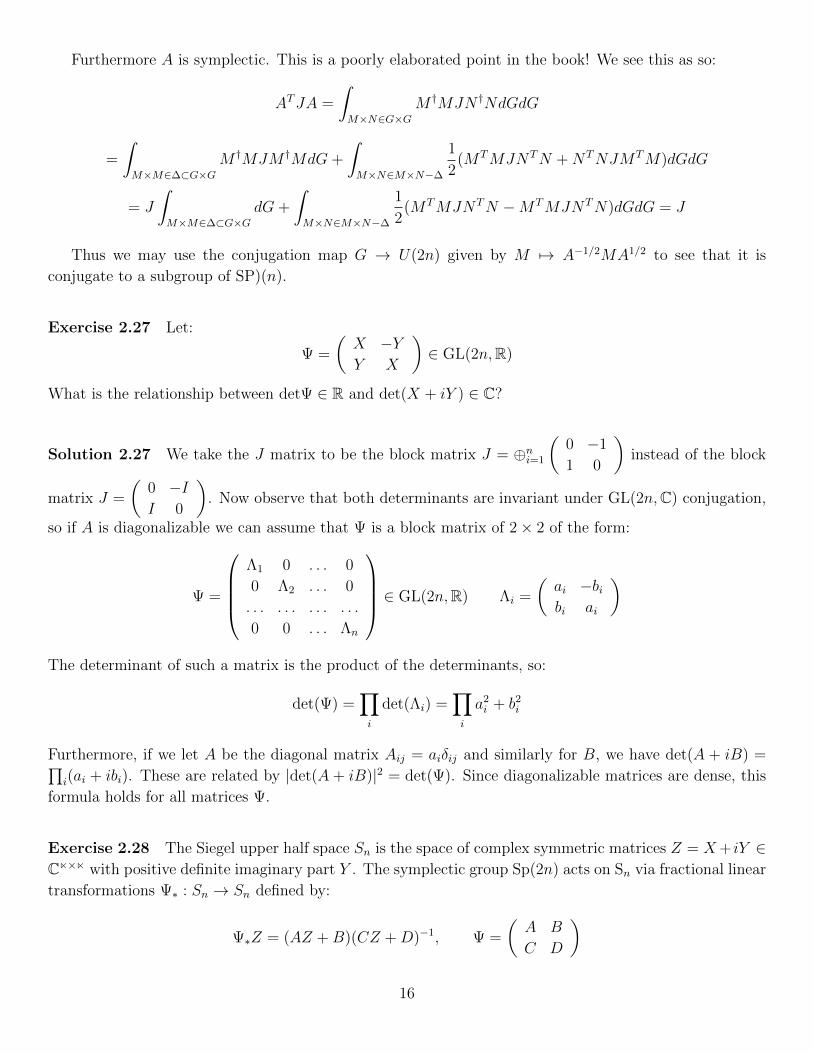
Exercise 2.27 Let:

Ψ =

(X −YY X

)∈ GL(2n,R)

What is the relationship between detΨ ∈ R and det(X + iY ) ∈ C?

Solution 2.27 We take the J matrix to be the block matrix J = ⊕ni=1

(0 −1

1 0

)instead of the block

matrix J =

(0 −II 0

). Now observe that both determinants are invariant under GL(2n,C) conjugation,

so if A is diagonalizable we can assume that Ψ is a block matrix of 2× 2 of the form:

Ψ =

Λ1 0 . . . 0

0 Λ2 . . . 0

. . . . . . . . . . . .

0 0 . . . Λn

∈ GL(2n,R) Λi =

(ai −bibi ai

)

The determinant of such a matrix is the product of the determinants, so:

det(Ψ) =∏i

det(Λi) =∏i

a2i + b2

i

Furthermore, if we let A be the diagonal matrix Aij = aiδij and similarly for B, we have det(A + iB) =∏i(ai + ibi). These are related by |det(A + iB)|2 = det(Ψ). Since diagonalizable matrices are dense, this

formula holds for all matrices Ψ.

Exercise 2.28 The Siegel upper half space Sn is the space of complex symmetric matrices Z = X+ iY ∈Cn×n with positive definite imaginary part Y . The symplectic group Sp(2n) acts on Sn via fractional linear

transformations Ψ∗ : Sn → Sn defined by:

Ψ∗Z = (AZ +B)(CZ +D)−1, Ψ =

(A B

C D

)

16

Here we use the notation of Exercise 1.13. Prove that Φ∗ is well-defined: if Z ∈ Sn then the matrix is

CZ +D is invertible and Ψ∗Z ∈ Sn. Prove that:

Ψ∗Φ∗Z = (ΨΦ)∗Z

for Φ,Ψ ∈ Sp(2n) and Z ∈ Sn. Prove that the action is transitive. Prove that:

Ψ(iI) = iI ⇐⇒ Ψ ∈ U(n)

Deduce that the map Ψ→ Ψ∗(iI) induces a diffeomorphism from the homogeneous space Sp(2n)/U(n) to

the Seigel upper half space Sn. Thus the quotient Sp(2n)/U(n) inherits the complex structure of Sn.

Solution 2.28 We prove everything except that the maps are well-defined, which we postpone until the

end. First observe that if:

Ψ =

(A B

C D

)Φ =

(E F

G H

)ΦΨ =

(EA+ FB EB + FD

GA+HC GB +HD

)Then we have:

Φ∗Ψ∗Z = (E(AZ +B)(CZ +D)−1 + F )(G(AZ +B)(CZ +D)−1 +H)−1

= (E(AZ +B) + F (CZ +D))(CZ +D)−1((G(AZ +B) +H(CZ +D))(CZ +D)−1)−1

= (E(AZ +B) + F (CZ +D))(G(AZ +B) +H(CZ +D))−1

= ((EA+ FC)Z + (EB + FD))((GA+HC)Z + (GB +HD))−1 = (ΦΨ)∗Z

So the map is a group homomorphism into complex automorphisms of Sn.

To see the group is transitive, it suffices to check that the map sp(2n) → TZSn induced by the group

representation is surjective. This then implies that the group action is locally transitive in a neighborhood

of any Z ∈ Sn, and then by a continuity argument and the fact that Sn is connected we may conclude that

the group action is in fact globally transitive.

We thus need to check that for any N ∈ TZSn (i.e an N = U + iV with U, V symmetric) there is a

family of symplectic maps ddt

(Φt)|t=0 = S with S ∈ sp(2n) with ddt

((Φt)∗Z) = N . Recall that sp(2n) can

be described as the set of matrices splitting into blocks A,B,C,D in the obvious way with D = −AT ,

B = BT and C = CT . Now observe that:

d

dt((Φt)∗Z)|t=0 =

d

dt((Z + t(AZ +B) +O(t2))(tCZ + +1 + tD +O(t2))−1)|t=0

=d

dt((Z + t(AZ +B) +O(t2))(1− t(CZ +D) +O(t2)))|t=0

= AZ +B − ZCZ − ZD = AZ + ZAT +B − ZCZ

Thus we just need to prove that we can pick an A,B,C,D satisfying the above identities (to be in sp(2n))

such that AZ+ZAT +B−ZCZ = U + iV . We can assume C = 0. Then in terms of Z = X+ iY we want

17

AX + B + XAT = U and AY + Y AT = V . Here B is symmetric and A can be anything. But since the

map A 7→ AY + Y AT is the composition of the map A → Y A (which is a bijection because Y is positive

definite) and the symmetrization map P 7→ P +P T we know that it is surjective. So we can certainly pick

an A. Then we may simply pick B = U − AX − XAT , D = −AT and C = 0 to find the S ∈ sp(2n) of

interest. This proves transitivity.

Now we identify the stabilizer of a point. We pick i1. Then we see that we want to find symplectic Ψ

so that the blocks A,B,C,D satisfy:

(iA+B)(iC +D)−1 = i1; iA+B = −C + iD;B = −C,A = D

This is in fact the condition that ΨJ = JΨ. Thus Ψ is in the stabilizer of i1 if and only if Ψ ∈ GL(n,C)∩Sp(2n) = U(n). Since we have in general that a space H with a transitive group action G is diffeomorphic

to G/Stab(p).

Exercise 2.32 Prove that the orthogonal compliment of a Lagrangian subspace Λ ⊂ R2n with respect

to the standard metric is given by Λ⊥ = JΛ. Deduce if u1, . . . , un is an orthonormal basis of Λ then the

vectors u1, . . . , un, Ju1, . . . , Jun forms a basis for R2n which is both symplectic and orthogonal. Relate this

to the proof of Lemma 2.31.

Solution 2.32 Since J is orthogonal, the vectors Ju1, . . . , Jun are independent from each other. Now

observe that since ω(v, w) = 〈v, Jw〉, we see that ω(ei, ej) = ω(Jei, Jej) = 〈ei, Jej〉 = 0 and 〈ei, ej〉 =

〈Jei, Jej〉 = −ω(Jei, ej) = −δij. These calculations show that the set e1, . . . , en, Je1, . . . , Jen are a set of

2n orthonormal (thus an orthonormal basis) and standard with respect to the symplectic form.

One way to interpret this in terms of Lemma 2.31 is to note that this elucidates the relationship between

the Lagrangian and its perpendicular Lagrangian, relating them via the unitary transformation J .

Exercise 2.33 State and prove the analog of Lemma 2.31 for isotropic, symplectic and coisotropic

subspaces.

Solution 2.33 (i) We prove that if V is isotropic, coisotropic or symplectic then so is ΨV for any

symplectic map. This is clear: ω(v, w) = 0 for all v ∈ V and some w if and only if ω(Ψv,Ψw) = 0. Thus

(ΨV )ω = ΨV ω and V ω ⊂ V (resp. V ⊂ V ω) if and only if (ΨV )ω ⊂ ΨV (resp. ΨV ⊂ (ΨV )ω). Likewise if

ω|V is non-degenerate then ω|ΨV = Ψ∗ω|ΨV is as well.

(ii) We prove that symplectic maps are transitive on isotropic, symplectic and coisotropic subspaces of

the same rank. First suppose that V is isotropic of rank k ≤ n. Then we can pick a Lagrangian L with

V ⊂ L and a matrix:

M =

[X

Y

]with orthogonal columns forming a basis of L, and where the first k columns form a basis of V . Then the

18

matrix: [X −YY X

]is a map taking the isotropic space spanned by e1, . . . , ek to V . Note that Ψ is in fact unitary.

For the coisotropic case, where the rank of V is k ≥ n, we can simply observe thav V ω is isotropic

and find a symplectic Ψ taking V ω to the standard rank 2n − k isotropic space as above. Then since

(ΨV ω)ω = ΨV we may conclude that V goes to the symplectic perpendicular of the standard rank 2n− kisotropic space. Again, Ψ here is unitary.

Finally, if V is symplectic of rank 2k then we can take a symplectic bases g1, h1, . . . , gk, hk for V and

gk+1, hk+1, . . . , gn, hn for V ω, and then use the map Φ given by gi 7→ ei, hi 7→ fi.

(iii) Finally, we characterize these Grassmanians as homogeneous spaces. The symplectic case of

SGr(n, k) is simple enough: the stabilizer of a symplectic subspace of rank k is isomorphic to the symplectic

group Sp(2k) so SGr(n, k) ' Sp(2n)/Sp(2k). For the isotropic case, IGr(n, k), we observe that any choice

of X + iY ∈ U(n) yields a rank k isotropic space as the span V the first k columns of M (where M is

as above). Two such M yield the same V if and only if they are related by right multiplication by an

element of O(k)×O(n− k) (an orthogonal transformation preserving the span of the first k columns and

their ortho-compliment). So we have IGr(n, k) ' U(n)/O(k)×O(n−k). Finally, for coisotropic CGr(n, k)

we use duality via taking the symplectic perp to see that CGr(n, k) ' IGr(n, 2n − k) ' IGr(n, k) 'U(n)/O(2n− k)×O(k − n).

Exercise 2.34 Consider the vertical Lagrangian:

Λvert = z = (x, y) ∈ R2n|x = 0

Use Lemma 2.30 to show that L(n) is the disjoint union:

L(n) = L0(n) ∪ Σ(n)

where L0(n) can be identified with the affine space of symmetric n × n matrices and Σ(n) consists of all

Lagrangian subspaces which do not intersect Λvert transversely. The set Σ(n) is called the Maslov cycle.

Solution 2.34 We simply prove that a Lagrangian L can be given as a graph over Λhor if and only

if it is transverse to Λvert. But observe that Λvert = JΛhor = (Λhor)⊥. Furthermore an n-dimensional

subspace V of R2n can be described as a graph over Λhor if and only if orthogonal projection V → Λhor is

an isomorphism, i.e has no kernel. But the kernel of this map is precisely V ∩ Λvert. So there is no kernel

if and only if V ∩ Λvert = 0, i.e if and only if V and Λvert are transverse.

Exercise 2.36 The Maslov index of a loop Λ : R/Z → L(V, ω) of a Lagrangian subspace in a general

symplectic vector space is defined as the Maslov index of the loop t 7→ Ψ−1Λ(t) ∈ L(n), where Ψ :

(R2n, ω0) → (V, ω) is a linear symplectomorphism. Show that this definition is independent of Ψ. Show

that if one reverses the sign of ω then the sign of the Maslov index reverses also.

19

Solution 2.36 For the first part, simply observe that if Ψ,Φ : (R2n, ω0) → (V, ω) are two different

symplectomorphisms then Ψ−1Λ(t) = Ψ−1Φ(Φ−1Λ(t)). Thus if we denote the constant path t 7→ Ψ−1Φ as

Ψ−1Φ then we have µ(Ψ−1Φ) = 0 and therefore:

µ(Φ−1Λ) = µ(Ψ−1Λ) + 2µ(Ψ−1Φ) = µ(Ψ−1Λ)

by the composition axiom. This shows that if (U, ω) and (V, ω′) are two symplectic vectorspaces, Ψ : U → V

is a symplectomorphism and Λ : R/Z→ L(U, ω) is a path of Lagrangians, then µ(Λ) = µ(ΨΛ).

For the second part, by the previous argument we may reduce to the case of (R2n, ω0) and (R2n,−ω0).

It suffices to check that Maslov index for the generating homotopy class, Λ0(t) ⊕ Rn−1 ⊂ C ⊕ Cn−1 with

Λ0(t) = e2πitR changes sign, and due to the direct sum formula it even suffices to check for Λ0(t). The

isomorphism c : (C, ω0)→ (C,−ω0) is just conjugation z 7→ z, so under this map the family Λ0(t) = e2πitRgets sent to cΛ0(t) = e−2πitR. This is the same curve with the reverse parameterization, thus µ(cΛ) =

µ(Λ(−·)) = −µ(Λ).

Exercise 2.37 Let Ψ : R/Z → Sp(V, ω) be a loop of linear symplectomorphisms. Prove that the

corresponding loop ΓΨ : R/Z→ L(V × V, (−ω)× ω) of Lagrangian graphs has twice the Maslov index, i.e

µ(ΓΨ) = 2µ(Ψ).

Solution 2.37 We see that Λ(t) = v ⊕ Ψ(t)v|v ∈ V = (1 ⊕ Ψ(t))Λ0(t) where Λ0(t) = v ⊕ v|v ∈ V and 1⊕Ψ(t) is the family of symplectomorphisms given by v ⊕ w 7→ v ⊕Ψ(t)w. Thus we have:

µ(Λ(t)) = µ(Λ0(t)) + 2µ(1⊕Ψ(t)) = 0 + 2(µ(1) + µ(Ψ(t))) = 2µ(Ψ(t))

Here we apply the product axiom, then the direct sum axiom, then the homotopy axiom.

Exercise 2.40 Prove that every anti-symplectic linear map has determinant (−1)n. Prove that every

anti-symplectic linear map preserves the linear symplectic width of subsets of R2n.

Solution 2.40 For the first part, suppose that Ψ is anti-symplectic. Then:

(−1)nωn = (−ω)n = (Ψ∗ω)n = det(Ψ)ωn

So det(Ψ) = (−1)n. Here by ωn we mean the nth wedge power of ω.

For the second part, consider a subset A ⊂ R2n. We observe that a ball B2n(r) can be mapped into A

via a symplectic map if and only if it can be mapped in via an anti-symplectic map. Indeed, we have the

standard involutive anti-symplectic map Φ given by ei 7→ fi, fi 7→ ei which fixes any ball B2n(r). Thus if

we have an affine symplectic (resp. anti-symplectic) ψ : B2n(r)→ A then ψ Φ is an affine anti-symplectic

(resp. symplectic) map B2n(r)→ A.

Now for an anti-symplectic affine map ψ consider ψ(A). Then if ξ : B2n(r) → A were an affine

symplectic map to A, then ψξΦ is a symplectic map B2n(r) → ψ(A). Furthermore if ξ : B2n(r) → ψ(A)

20

is symplectic, then ψ−1ξΦ is a symplectic map B2n(r)→ A. Thus we have:

w(A) = supπr2|ψ(B2n(r)) ⊂ A for some ψ ∈ ASp(R2n)

= supπr2|ξ(B2n(r)) ⊂ ψ(A) for some ξ ∈ −ASp(R2n) = w(ψ(A))

Exercise 2.46 Let E ⊂ R2n be an ellipsoid and define the dual ellipsoid by:

E∗ = v ∈ R2n|〈v, e〉 ≤ 1∀e ∈ E

where 〈·, ·〉 is the standard inner product on R2n. Prove that:

E∗∗ = E, (ΨE)∗ = (ΨT )−1E∗

for Ψ ∈ Sp(2n).Prove that the symplectic spectrum of E∗ is given by (1/rn, . . . , 1/r1) where (r1, . . . , rn) is

the symplectic spectrum of E. Deduce that the dual of a linear symplectic ball is again a linear symplectic

ball.

Solution 2.46 First we show that (ΨE)∗ = (ΨT )−1E∗. Indeed, we see that:

〈v, e〉 = 〈v,Ψ−1Ψe〉 = 〈(Ψ−1)Tv,Ψe〉

Thus 〈v, e〉 ≤ 1 for all e ∈ E if and only if 〈(Ψ−1)Tv,Ψe〉 ≤ 1 for all Ψe ∈ ΨE. This implies that E∗ and

(ΨE)∗ are symplectomorphic. Thus it suffices to show that E = E∗∗ for standard ellipsoids, which will

follow from the last statement.

Now suppose that E has spectrum (r1, . . . , rn). Then E = e|〈e, Re〉 ≤ 1 where R = diag(r1, . . . , rn).

Now suppose that v ∈ E where E = v|〈v,R−1v〉 ≤ 1. Then for any e ∈ E we have:

|〈v, e〉|2 = 〈R−1/2v,R1/2e〉 ≤ 〈v,R−1v〉〈e, Re〉 ≤ 1

Thus v ∈ E∗. If on the other hand 〈v,R−1v〉 = c > 1 and e 6∈ E then w = c−1/2R−1v satisfies:

〈w,Rw〉 = c−1〈R−1v,RR−1v〉 = c−1〈v,R−1v〉 = 1

Thus w ∈ E. But then we have:

〈w, v〉 = c−1/2〈v,R−1v〉 = c1/2 > 1

so e 6∈ E∗. Thus E = E∗ and we are done.

Exercise 2.49 Let (V, ω) be a symplectic vector space and J be a complex structure on V . Prove that the

following are equivalent. (i) J is compatible with ω. (ii) The bilinear form gJ(v, w) = ω(v, Jw) is symmetric,

positive definite and J-invariant. (iii) The form H : V ×V → C given by H(v, w) = ω(v, Jw) + iω(v, w) is

21

complex linear in w, complex anti-linear in v, satisfies H(w, v) = H(v, w) and has a positive definite real

part.

Solution 2.49 (i) =⇒ (ii). We have:

gJ(v, w) = ω(v, Jw) = −ω(Jw, v) = −ω(J2w, Jv) = ω(w, Jv) = gJ(w, v)

so gJ is symmetric. Also gJ(v, v) = ω(Jv, Jv) > 0 unless v = 0 and:

gJ(Jv, Jw) = ω(Jv, J2w) = −ω(Jv, w) = ω(w, Jv) = gJ(w, v) = gJ(v, w)

So gJ is positive definite and J-invariant.

(ii) =⇒ (iii). We evidently have H(u + v, w) = H(u,w) + H(v, w) and likewise for the other entry

since H is a sum of R-bilinear maps. Now if c = x+ iy ∈ C we have:

H(cv, w) = gJ(cv, w) + iω(cv, w) = gJ(xv + yJv, w) + iω(xv + yJv, w)

= xgJ(v, w) + ygJ(Jv, w) + ixω(v, w)− iyω(w, Jv)

= xgJ(v, w) + ygJ(v, Jw) + ixω(v, w)− iygJ(w, v)

= xgJ(v, w)− yω(v, w) + ixω(v, w)− iygJ(v, w)

= (x− iy)(gJ(v, w) + iω(v, w)) = cH(v, w)

Notice that we are careful to only use the compatibility between gJ and J here, which are guaranteed by

(i). A nearly identical calculation shows H(v, cw) = cH(v, w). We also have:

H(w, v) = gJ(w, v) + iω(w, v) = gJ(v, w)− iω(v, w) = H(v, w)

Finally we see that H(v, v) = gJ(v, v) + iω(v, v) = gJ(v, v) > 0 unless v = 0.

(iii) =⇒ (i). For any v 6= 0 we have ωJ(v, Jv) = gJ(v, v) = H(v, v) > 0 if (iii) holds. Furthermore:

ω(Jv, Jw) =1

2(H(iv, w) +H(iv, w)) =

1

2(−iH(v, w) + (iH(v, w))) =

−i2

(H(v, w)−H(v, w)) = ω(v, w)

Exercise 2.52 (i) Prove the continuity of the map r : Met(V )→ J (V, ω) in Proposition 2.50 as follows.

If V = R2n and ω = ω0 then an inner product g ∈Met(R2n) can be written in the form g(v, w) = wTGv

where G ∈ R2n×2n is positive definite. The formula w0(v, w) = (J0v)Tw = g(Av,w) determines the matrix

A = G−1J0. Prove that the g-adjoint of A represented by the matrix A∗ = G−1ATG = −A. Prove that

tghe g-square root of the matrix P = A∗A = −A2 = G−1JT0 G−1J0 is given by:

Q = G−1/2(G−1/2JT0 G−1J0G

−1/2)1/2G1/2

Deduce that the map G→ JG = Q−1G−1J0 is continuous.

(ii) The algebra here is also just a reformulation of that in the proof of Lemma 2.42. Use the current

22

method to give an alternative proof of this result.

(iii) Deduce from (ii) that a complex structure J is ω-compatible if and only if it has the form J =

Ψ−1J0Ψ for some Ψ ∈ Sp(2n).

Solution 2.52 (i) We observe that for any v, w we have:

g(Av,w) = vTATGw = vTGG−1ATGw = g(v,G−1ATGw) = g(v, A∗w)

Thus we must have A∗ = G−1ATG. Furthermore:

g(v,Aw) = −g(w,Av) = −g(A∗w, v) = g(v,−A∗w)

so A∗ = −A. Now consider P = A∗A = G−1ATGA. We have that R = G1/2PG−1/2 = G−1/2ATGAG−1/2

is a symmetric positive definite matrix, and thus R = OTΛO for some orthogonal O and diagonal positive

Λ. We may thus define the square root as R1/2 = OTΛ1/2O. Note that the map R→ R1/2 can be defined

around any multiple of the identity λI with λ > 0 using the Taylor series for√λ+ x, which has radius of

convergence λ. Thus we can see that R→ R1/2 is a continuous (in fact, smooth!) function of the entries of

R by noting that R1/2 = (λI+(R−λI)1/2 (where the right-hand side is defined using the Taylor expansion

about λ) for λ greater than any eigenvalue of R. A similar discussion holds for the map M → M−1 (in

fact we can use the formula M−1 = det(M)−1 · adj(M) which show that M−1 can be written in terms of

smooth functions in the entries of M when M isn’t singular).

Thus the map G → Q = G−1/2R1/2G1/2 = G−1/2(G−1/2JT0 G−1J0G

−1/2)1/2G1/2 is smooth and we just

need to verify that Q satisfies all of the properties we want. We certainly have Q2 = G−1/2RG1/2 = P .

Furthermore we have:

g(v,Qw) = vTGG−1/2R1/2G1/2w = vTG1/2R1/2G1/2w = vT (G1/2R1/2G1/2)Tw = g(Qv,w)

Finally we see that sinceR is positive, R1/2 is positive and thusQ is because it is conjugate toR1/2. Thus the

Q given by the above formula is the g-square root, and we may conclude that the map G→ JG = Q−1G−1J0

is smooth due to it being a matrix product of smooth matrix-valued functions of the entries of G.

(ii) Let zj = uj ± ivj and ±iλj (with λi > 0) be the eigenvectors and eigenvalues of A = G−1J0.

Since A is real and anti-self-conjugate with respect to g, A must have imaginary eigenvalues coming in

conjugate pairs, with corresponding eigenvectors uj ± ivj which are g orthonormal. In this diagonal basis

Q = (A∗A)1/2 is the simply the diagonal matrix with entries λi. Now observe that A(uj+ivj) = λj(iuj−vj),soAuj = −λjvj, Avj = λjuj. Thus JGuj = Q−1Auj = −vj and JGvj = uj. In other words, this is a standard

basis for JG. Furthermore we have:

ω(vi, uj) = g(Avi, uj) = g(λiui, uj) = λiδij

and similarly ω(ui, vj) = −λiδij, ω(vi, vj) = ω(ui, uj) = 0. Thus we may set ei = λ−1i vi, fi = λ−1

i ui to get

a standard basis for ω which is g-orthogonal. Note that in this basis JG is still standard, since the change

of basis ui, vi → ei, fi commutes with JG (it is essentially just rescaling on the eigenspaces).

23

(iii) If J = Ψ−1J0Ψ for some Ψ ∈ Sp(2n), then:

ω(v, Jw) = 〈v, JT0 Ψ−1J0Ψw〉 = 〈v,ΨTJT0 J0Ψw〉 = 〈v,ΨTΨw〉

Thus ω(·, J ·) is positive definite. Furthermore ω(Jv, Jw) = ω(v, w) because J is a composition of three

symplectomorphisms. Conversely, suppose J is ω-compatible. Then by the work in (ii) it is conjugate to

J0 via a symplectic transformation (given by the basis ei and fi).

Exercise 2.53 Here is yet another proof of the contractibility of J (V, ω). This proof illustrates in a clear

geometric way the relationship between Lagrangian subspaces, complex structures and inner products.

Given a Lagrangian subspace Λ0 ∈ L(V, ω) there is a natural bijection:

J (V, ω)→ L0(V, ω,Λ0)× S(Λ0)

where L0(V, ω,Λ0) is the space of all Lagrangian subspaces which intersect Λ0 transversely and S(Λ0) is

the space of all positive definite quadratic forms on Λ0. Note that, by Lemma 2.30, the space L0(V, ω,Λ0)

is contractible. The above correspondence is given by the map:

J 7→ (JΛ0, gJ |Λ0)

where gJ(v, w) = ω(v, Jw) as above. Show that this map is a bijection.

Solution 2.53 First we show injectivity. First we see that ω(v, Jw) = ω(v, Iw) for any v, w ∈ Λ0.

Similarly, for any v ∈ JΛ0 = IΛ0 and w ∈ Λ0 we have:

ω(v, Jw) = ω(Jv′, Jw) = ω(v′, w) = 0 = ω(v′′, w) = ω(Iv′′, Iw) = ω(v, Iw)

where v = Jv′ = Iv′′ and v′, v′′ ∈ Λ0. But Λ0 and JΛ0 = IΛ0 span V . So ω(v, Jw) = ω(v, Iw) for any

v ∈ V and w ∈ Λ0, and it follows that Jw = Iw. Furthermore, suppose that Iv = Jw for some v, w ∈ JΛ0.

Then v = Iv′ and w = Jw′ for some v′, w′ ∈ Λ0. Furthermore:

−v′ = I2v′ = Iv = Jw = J2w′ = −w′

So v′ = w′. But then v = Iv′ = Jw′ = w, so v = w. Since J and I carry JΛ0 to Λ0 bijectively, this implies

that they agree on both JΛ0, i.e Jv = Iv for v ∈ JΛ0. Since Λ0 and JΛ0 together span V , this implies

that they agree on V .

Now we prove surjectivity. To see this, simply note that given a Lagrangian Λ transverse to Λ0 and a

metric g on Λ0, we have an isomorphism induced by ω, Λ→ Λ∗0, given by w 7→ ω(·, w). We may therefore

define J as a map Λ0 → Λ by the identity:

ω(v, Jw) = g(v, w)

i.e J : Λ0 → Λ is the unique map such that ω(·, Jw) = g(·, w) ∈ Λ∗0. We may then extend this to a map

J : V → V by defining Jv = Jv for v ∈ Λ0, Jv = −J−1v for v ∈ Λ, and then extending by linearity. We

24

may also extend g simply by setting g(v, w) = g(Jv, Jw) for v, w ∈ Λ and g(v, w) = 0 if v ∈ Λ0, w ∈ Λ.

We then have that Λ and Λ0 are perpendicular subspaces with respect to g. Furthermore, J2 = −1 and

g(v, w) = g(Jv, Jw) (this is easily checked on a split basis in V = Λ0 ⊕ Λ).

Exercise 2.54 Let ω and g be given. Show that there is a basis for V which is both g-orthogonal and

ω standard if and only if there is a Lagrangian subspace Λ whose g-orthogonal compliment Λ⊥ is also

Lagrangian.

Solutuion 2.54 If there is such a basis e1, . . . , en, f1, . . . , fn, then we can take Λ = span(ei) and Λ⊥ =

span(fi). Conversely, if two such Lagrangians exist, then we can construct such a basis via a version of

the symplectic Graham-Schmidt. More specifically, we can proceed by induction: if V is 2-dimensional,

we can pick the orthogonal basis e ∈ Λ, f ∈ Λ⊥, picking e arbitrarily and f so that ω(e, f) = 1, which we

must be able to do since Λ⊥ is transverse to Λ. If dim(V ) = 2n, then we pick an arbitrary non-zero e ∈ Λ.

Then there is a unique vector

Exercise 2.55 Let J ∈ J (V, ω). prove that a subspace Λ ⊂ V is Lagrangian with respect to ω if and only

if JΛ is the orthogonal compliment of Λ with respect to the inner product gJ . Deduce that Λ ∈ L(V, ω) if

and only if JΛ ∈ L(V, ω).

Solution 2.55 We see that:

ω(v, w) = 0 for all v, w ∈ Λ ⇐⇒ gJ(v, Jw) = −ω(v, JJw) = −ω(v, w) = 0 for all v ∈ Λ, Jw ∈ JΛ

By dimension counting, then, we must have Λ⊥ = JΛ. Since JΛ = Λ⊥ if and only if J2Λ = Λ = (JΛ)⊥,

we see that Λ is a Lagrangian if and only if JΛ is.

Exercise 2.56 Suppose that Jt is a smooth family of complex structures on V depending on a parameter

t. Prove that there exists a smooth family of isomorphisms Φt : R2n → V such that JtΦt = ΦtJ0.

Solution 2.56 Let I = (0, 1) be the open interval. Consider J(t) : V ⊗ C → V ⊗ C and consider the

sub-bundle E → I of I×V ⊗C→ I defined by E(t) = ker(J(t)− i1) ⊂ V ⊗C. This is a vector-bundle over

the interval, so it is trivial. Therefore we can pick n non-vanishing, linearly independent global sections

uj(t) + ivj(t). Point-wise these uj and vj satisfy J(t)(uj(t) + ivj(t)) = iuj(t) − vj(t), so J(t)vj(t) = uj(t)

and J(t)uj(t) = −vj(t). Using the map V ⊗ C ' V ⊕ iV → V given by u + iv → u + v, we may identify

the sections ui(t), Jui(t) = vi(t) as 2n sections of V . They are point-wise linearly independent, since the

vectors ui + iJui and ui − iJui were independent in the complexification. Thus the map Φt : R2n → V

given by ei → ui(t), fi → vi(t) gives the desired family of isomorphisms.

Note that if Jt were compatible with ω0 (the standard form, not time-dependent) then we could have

chosen Φt to be symplectic. Indeed, in that case, we can pick ui + ivi to be orthogonal with respect to

gJt = ω(·, Jt·) via the argument in Paragraph 2 of Solution 2.61, and the resulting map described above

would then be symplectic since then ω(ui, vi) = gJ(ui, Jvi) = gJ(ui, ui) = 1 and ω(ui, ui) = ω(vi, vi) = 0.

25

Finally, this argument can be extended to a family Jt of complex structures on a trivial bundle E =

U×R2k over U , to show that there is a family of bundle automorphisms Φt : E → E such that JΦt = ΦtJ0.

We may or may not take Jt compatible with ω0; in the latter case, which case we may take Φt to be

automorphisms of E as a symplectic bundle. Again, the same argument as above will work, except this

time we pick sections uj + ivj over I × U .

Exercise 2.57 Prove that the real 2× 2 matrix:

J =

(a b

c d

)satisfies J2 = −1 if and only if det(J) = 1 and a = −d. Deduce that J0 and −J0 lie in different components

of J (R2). Prove that each component of J (R2) is contractible.

Solution 2.57 J2 = −1 implies that the eigenvalues are ±i, and since imaginary eigenvalues for real

matrices occur in conjugate pairs, this implies that there must be 1 i eigenvalue and 1 −i eigenvalue.

Therefore J2 = −1 if and only if det(J − λ) = λ2 − tr(J) + det(J)λ2 + 1. This proves the first part.

To prove the second part, we recall that J (R2) ' GL(2,R)/GL(1,C) with connected components

distinguished by the determinant. Thus if two complex structure are related by an orientation reversing

transformation, then they are in separate components. Indeed, J0 and −J0 are related by the transforma-

tion e1 → e2, e2 → e1, which is determinant −1. So they are in different components.

To prove the third part, we observe that there exists a G ∈ GL+(2,R) is connected: these matrices can

be retracted via ht(M) = (MMT )−t/2M to SO(2) = U(1), which is certainly connected. Thus there exists

a family of maps M(t) such that the path J(t) = M(t)J0M(t)−1 has J0 = J(0) and J = J(1) for any J in

the component of J0.

Exercise 2.58 Let V be a 2n-dimensional real vector space with complex structure J . Show that the

space of all skew-forms ω which are compatible with J is convex.

Solution 2.58 Simply observe that if ω0, ω1 are two such forms, then ω(t) = tω0 + (1 − t)ω1 is anti-

symmetric. Furthermore gω(t) = tgω0 +(1− t)gω1 and metrics are convex, so ω(t)(·, J ·) is certainly a metric.

This also means that ω(t) is non-degenerate, since ω(t)(v, Jv) > 0 for all v 6= 0, so ω(t) : V → V ∗ is

injective. This proves that any convex combination of compatible forms is compatible.

Exercise 2.59 A linear subspace W ⊂ V is called totally real if it is of dimension n and:

JW ∩W = 0

If W ⊂ V is a totally real subspace show that the space of non-degenerate skew forms ω : V ×V → R which

are compatible with J and satisfy W ∈ L(V, ω) is naturally isomorphic to the space of inner products on

W and hence is convex.

26

Solution 2.59 We define the map as so. First, let πΛ denote projection to Λ along JΛ. Then we can

define a metric g on V from a metric g on W via:

g(v, w) = g(πΛv, πΛw) + g(πΛJv, πΛJw)

This metric is J-invariant, restricts to g on W and has Λ ⊥ JΛ, and it’s easy to see that it is the unique

metric satisfying these properties. Now we define the map

ωg(v, w) = −g(v, Jw) = −g(πΛv, πΛJw) + g(πΛJv, πΛw)

Now we have

ωg(v, w) = g(v, Jw) = −g(Jv, w) = −g(w, Jv) = −ωg(w, v)

Thus ωg is an anti-symmetric. It is also non-degenerate, since ωg(v, Jv) = g(v, v) > 0 for any v 6= 0.

Finally, we have:

ωg(v, w) = −g(v, 0) + g(0, w) = 0

for v, w ∈ Λ and likewise for JΛ by J invariance. So both Λ and JΛ are Lagrangian, and this defines a

map Ψ : Met(W ) → Symp(M) which maps metrics on W into compatible symplectic forms on V which

have W as a Lagrangian. This map is clearly injective, since if we have two metrics g, h on Λ and v, w ∈ Λ

with g(v, w) 6= h(v, w), then ωg(v, Jw) 6= ωh(v, Jw). Furthermore, the formula for ωg is smooth in g.

Conversely, to see surjectivity, we consider any ω satisfying those properties with respect to W . We

can take the metric gJ = ω(·, J ·) and see that it is a J-invariant metric, restricting to h = gJ |Λ on Λ and

having Λ ⊥ JΛ. Thus we have h = g and thus ωh = ω, so Ψ(h) = ω, and the map Ψ is surjective. Note

that the map ω → gJ |Λ is the inverse to Ψ, and it is smooth, so the map Ψ is in fact a diffeomorphism.

Exercise 2.61 Prove that a symplectic vector bundle as defined on p. 69 is locally symplectically trivial.

Solution 2.61 We are given a rank 2k vector-bundle E → X over some base X with a smooth non-

degenerate section ω of E∗ ∧ E∗. Pick a metric h. Then there exists a unique anti-self-adjoint, invertible

section A of End(E) satisfying h(v,Aw) = ω(v, w). We may consider the section J = (A∗A)−1/2A =

(−A2)−1/2A. Here (A∗A)−1/2 is as in Solution 2.52, see that problem for a more thorough discussion.

We see that if we define g(v, w) = h(v, (A∗A)1/2w) then h is a new metric satisfying g(v, Jw) = ω(v, w).

Furthermore J2 = −1, so J has n i eigenvalues and n −i eigenvalues. Let K ⊂ E ⊗ C be defined as

K = ker(J − i1).

Now let p ∈ X be any point and U ' Bn ⊂ Rn be any simply connected neighborhood of p. Then

K|U is a line bundle over U , and thus is thus topologically trivial. Thus it possesses n independent global

sections zj = uj + ivj. In fact, we can make these orthonormal with respect to g|K (extended to E ⊗ Cas a Hermitian inner product then restricted to K). We may first pick a non-vanishing section u1 + iv1 of

K|U , then setting K1 = span(u1 + iv1) pick a section u2 + iv2 in K1|⊥U (which is also trivial), then define

K2 = span(u1 + iv1, u2 + iv2) and proceed thus. Note that the real sections ui are perpendicular in E due

to this choice.

By the standard argument (see Solution 2.11) we have Aui = −vi, Avi = ui. Thus via the map E⊗C '

27

E⊕iE → E via u+iv → u+v we get 2n independent real sections ui, Jui satisfying ω(ui, vj) = g(ui, Avj) =

δij and ω(ui, uj) = ω(vi, vj) = 0. Thus the map ψ : U×R2k → E|U given by (x, ei)→ vi(x), (x, fi)→ ui(x)

has the property that ψ∗ω = ω0 and constitutes a symplectic trivialization over U .

Exercise 2.64 Let E → M be a 2n-dimensional vector-bundle with complex structure J and F → ∂M

be an n-dimensional real sub-bundle. This means JqFq ∩ Fq = 0 for all q ∈ ∂M . Prove that there exists

a symplectic bilinear form ω which is compatible with J and satisfies Fq ∈ L(Eq, ωq) for q ∈ ∂M . Prove

that the space of such forms is contractible.

Solution 2.64 We apply an identical construction to that in Exercise 2.59. That is, define the following

fiber-bundle isomorphism Ψ : Met(F )→ SympJ,F (E). Here Met(F ) denotes the bundle whose fiber is the

metrics on Fp. SympJ,F (E) denotes the bundle whose fiber is the space of J-compatible symplectic forms

on E with F as a Lagrangian. We want the isomorphism:

Ψ(g) = ωg, ωg(v, w) := −g(πFv, πFJw) + g(πFJv, πFw)

Note that since J varies smoothly and F is a smooth sub-bundle, the section πF of End(E) to F along JF

is smooth. Thus the map Ψ is a smoothly varying map which is smooth as a map of the fibers. In fact, Ψ

can be extended to a section of Hom(E∗ ⊗ E∗, E∗ ∧ E∗) which is fiber-wise linear!

This map is an isomorphism on the fibers by Exercise 2.59. Furthermore, the fibers of Met(F ) are

convex, so since Ψ extends to a section of Hom(E∗ ⊗ E∗, E∗ ∧ E∗) we may conclude that the bundle

of symplectic forms also has convex fiber. A fiber-bundle with convex fiber has a contractible space of

sections, so the space Γ(SympJ,F (E)) is contractible. Furthermore, since Γ(Met(F )) is non-empty (we can

run the usual partition of unity argument) Γ(SympJ,F (E)) is also non-empty. So such an ω exists.

To prove existence once we know convexity, we could alternatively apply a partition of unity argument

directly to textSympJ,F (E). Namely, we take locally trivially patches Ui (where E|Ui is a trivial complex

vector bundle of rank 2n), find ωi on each patch by taking the standard one, and then taking convex

combinations of these ωi using a partition of unity to get a global ωi.

Exercise 2.67 Define the notion ‘symplectic trivialization.’ Show that a Hermitian line bundle has a

unitary trivialization if and only if its underlying symplectic bundle has a symplectic trivialization.

Solution 2.67 Let (E0, ω0, J0, g0)→ X denote the trivial Hermitian vector-bundle with E0 = X × R2k,

ω0(x) = ω0, J0(x) = J0, g0(x) = 〈·, ·〉 and π : E0 = X × R2k → X the standard projection map. We will

also use E0 to denote the underlying trivial symplectic bundle.

Let (E,ω) → X be a symplectic vector-bundle of rank 2k. A symplectic trivialization is a bundle

isomorphism Ψ : E0 → E with Ψ∗ω = ω0. Similary, let (E,ω, J, g) → X be a Hermitian vector-bundle of

rank 2k. A unitary trivialization is a bundle isomorphism Ψ : E0 → E with Ψ∗ω = ω0, JΨ = ΨJ0 and

Ψ∗g = g.

Evidently, a unitary trivialization of a unitary bundle is also a symplectic trivialization of the underlying

28

symplectic bundle. Now suppose that Ψ : (E0, ω0, J0, g0)→ (E,ω, J, g) is a symplectic trivialization. Then

J1 = Ψ−1JΨ and J0 are two complex structures on E0 which are compatible with ω0. By Solution 2.56,

there exists a symplectic bundle automorphism Φ : E0 → E0 (connected to the identity in fact) such that

J1Φ = ΦJ0. Thus ΨΦ has the property that (ΨΦ)∗ω = ω0 and JΨΦ = ΨΦJ0. By the compatibility

condition, it follows that (ΨΦ)∗g = g0. Thus this is a unitary trivialization of E.

Exercise 2.68 Prove that the space of paths Ψ : [0, 1] → Sp(2n) of symplectic matrices satisfying

Ψ(1) = Ψ(0)−1 has two components. Deduce that up to isomorphism there are precisely two symplectic

vector bundles (of every given dimension) over the real projective RP 2.

Solution 2.68 Let Ψ : [0, 1] → Sp(2n) be such a path. We single out two standard loops: Ψ0,Ψ1 :

[0, 1] → Sp(2n) where Ψ0(t) ≡ 1 and Ψ(0) = R(θ) ⊕ 12n−2 ∈ U(1) ⊕ Sp(2n − 2). Both of these Ψi are

evidently in our class of curves. We will show that every Ψ(t) is homotopic to exactly one Ψi.

First observe that any Ψ is homotopic to a curve such that Ψ(1) = Ψ(0). We can just take any curve

Φ(t) such that Φ(0) = 1 and Φ(1) = Ψ(1), letting Φs(t) denote the partial curve Φs(t) = Φ((1 − s) + st)

and Φ−1s (t) = Φ((1 − s) + s(1 − t))−1. Then Ψs = Φ−1

s Ψ Φs (where denotes path composition) is

a homotopy of curves with Ψs(0) = Ψs(1)−1 and Ψ1(0) = Ψ1(1) = 1. Thus we may consider without

loss of generality that Ψ(0) = Ψ(1) = 1 and we may classify homotopy classes of these (we will still use

homotopies of curves where Ψ(0) 6= Ψ(1)).

Now, if Ψ and Ψ′ are two such curves, and they are homotopic as curves S1 → Sp(2n) with 0 7→1, then they are evidently homotopic as curves with Ψ(0) = Ψ(1)−1. Now let Φ(t) = Ψ1(t), so that

[Ψ1] ∈ π1(Sp(2n)) = Z generates the group. Let Ψ1,s(t) and Ψ−11,s(t) be as Φs and Φ−1

s above. Then

Ψs = Ψ−11,s Ψ Φ1,s has [Ψ] = [Ψ] + 2[Ψ1] for any of our Ψ. Thus any curve is homotopic to a curve in the

π1 class of Ψ0 or Ψ1, and thus to Ψ0 or Ψ1 itself.

Conversely, suppose that Φs is a homotopy of curves with Φ0(0) = Φ0(1) = Φ1(0) = Φ1(1) = 1 and

Φs(0) = Φ−1s (1) for all s. Let Γ(t) = Φt(0) and let Γs and Γ−1

s be like Φs and Φ−1s above. Observe that Γ

itself is a closed curve, so [Γ] = [Γ1] = k[e] for some generator [e] of π1(Sp(2n)). Then Ψr = Γ−1r Φr Γr is

a homotopy of curves with Ψr(0) = Ψr(1) = 1. Thus we see that [Φ1] = [Φ0] + 2[Γ1] = [Φ0] + 2n[e]. Thus

the mod 2 homotopy class of a curve [Φ] with Φ(0) = Φ(1)−1 is invariant up to homotopy through other

such curves.

Thus we has established that there are two homotopy classes of our curves. Now consider a symplectic

vector bundle E → RP 2. We may take RP 2 and split it along a circle into a disk D2, where the boundary

S1 ' ∂D2 is identified with itself in RP 2 via the antipode map a : ∂D2 → ∂D2. E then pulls back to

the trivial bundle over D2, since it is over a disk, coupled with a bundle map Ψ : Ep → Ea(p). The data

of a line bundle over RP 2 is thus the data of a bundle map Φ : E|∂D2 → E|∂D2 identifying Ep with Ea(p),

and satisfying Φ(p) = Φ(a(p))−1. Identifying ∂D2 = R/2Z, such a map is given equivalently by a map

Ψ : [0, 1]→ Sp(2n) with Ψ(0) = Ψ(1)−1. We can then recover the original map Ψ : ∂D2 → Sp(2n) by path

composing Ψ Ψ.

Two different trivializations of E over D2 yield isotopic bundle maps on ∂D2. Indeed, any two such

trivializations are related by a bundle map Ψ : E|D2 → E|D2 . Since the space of such bundle maps

29

If Φ and Φ′ are two homotopic bundle maps on ∂D2, they yield isomorphic bundles.

Exercise 2.75 Use the formula (2.2) (the characterization as the Euler class) to calculate the first Chern

class of the normal bundle νCP1 in CP2.

Solution 2.75 We have the trivializations Φ1 : Σ1 × C → νCP 1 and Φ2 : Σ2 × C → νCP 1 given by

Φ1([1 : z1 : 0], w) = [1 : z1 : w] and Φ2([z2 : 1 : 0], w) = [z2 : 1 : w]. Consider the section given by

([1 : z1 : 0], 1) in the firsts patch and ([z2 : 1 : 0], z2) in the second patch. The transition map Φ−12 Φ1 sends

([1 : z1 : 0], 1) → [1 : z1 : 1] → [1/z1 : 1 : 1/z1] → ([1/z1 : 1 : 0], 1/z1) = ([z2 : 1 : 0], z2). So this is a

well-defined section. Furthermore it evidently intersects the zero section (identified with [z2 : z1 : 0]) at a

single point, where z2 = 0 in the second patch. The orientation of νCP1 is induced by the ambient space,

CP2, via a normal neighborhood and with this orientation the intersection is positive since the section is

locally the intersection of two holomorphically embedded CP1’s in CP2.

Exercise 2.76 Let L ⊂ Cn × CP n−1 be the incidence relation:

L = (z, l)|z ∈ l = (z1, . . . , zn; [w1, . . . , wn])|wjzk = wkzj∀j, k

The projection π : L → CP n−1 gives L the structure of a complex line-bundle over CP n−1. Show that

when n = 2 the first Chern number of L is −1, and hence calculate c1(L) for arbitrary n.

Solution 2.76 Consider the n = 1 case. We have two patches for L, each over one of the disks in CP 1:

([z, 1], λ)→ ([z, 1], λ(z, 1)) and ([1, z], λ)→ ([1, z], λ(1, z)). Calculating the transition map, we see that:

([z, 1], λ)→ ([z, 1], λ(z, 1)) = ([1, 1/z], zλ(1, 1/z))→ ([1, 1/z], λz) = ([1, w], w−1λ)

Thus the curve S1 → Sp(2) induced by this bundle is θ → e−2πiθ, i.e c1(L) = µ(Ψ) = −1. For any n > 2,

we see that the inclusion map CP 1 → CP n−1 is covered by a bundle LCP 1 → LCPn−1 . Thus if we use c1(L)

to now denote the map H2(CP n−1)→ Z we have 〈c1(L)|[CP 1]〉 = −1. But since H2(CP n−1) is generated

by [CP 1], this completely determines c1(L) as a map.

Exercise 2.77 Prove that every symplectic vector bundle over a Riemann surface decomposes as a direct

sum of 2-dimensional vector bundles.

Solution 2.77 First observe that given a Riemann surface Σ, we can produce a plane bundle ξ → Σ

with c1(ξ) = z ∈ Z for any z ∈ Z. To do so, we simply pick a curve C ⊂ Σ such that Σ − C has is

connected and has 2 boundary components. Then we consider the trivial bundle ξ0 over Σ − C. Given a

map γ : C → Sp(2) with µ(γ) = z, we may produce a bundle ξ over Σ by using two trivializations: one over

a cylinder/normal neighborhood U0 ⊂ Σ with C ⊂ U0 and U0 ' (−1, 1)×C and one over U1 = Σ−C ⊂ Σ.

The transition map on U1 ∩ U2 = V −C ' (−1, 0)×C ∪ (0, 1)×C = U12 ∪ U21 can be the identity on

U12. On U21 we can define it using the identification U21 ' C ∪ (0, 1): if (x, s) are coordinates with respect

30

to this diffeomorphism, then we want to use the transition map Φ(x, s) = γ(x).

Now let C1 = C. Take a set of n − 1 other splitting curves C2, . . . , Cn so that Σ − tiCi is a union

of two disconnected surfaces Σ1 and Σ2, each homeomorphic to a disc with n − 1 holes. Then using the

trivialization of ξ on Σ−C to induce a trivialization of ξ on Σ−tiCi, we see that the maps Ψi : Ci → Sp(2)

given by the transition maps at the cycles are the identity for i > 1 and equal to γ for i = 1. Thus by

construction∑

i µ(Ψi) = z.

Now to answer the question. If we are given an arbitrary vector-bundle E of rank k, then c1(E) = z ∈ Z.

Pick any set of k integers zi so that∑

i zi = z, and let ξi be bundles with those Chern numbers, i.e

c1(ξi) = zi. Then the direct sum bundle F = ⊕iξi has c1(F ) =∑

i c1(ξi) =∑

i zi = z. So its rank and

Chern number agree with E, and by naturality we conclude that F ' E.

Exercise 2.78 (i) Suppose that E → Σ is a symplectic vector bundle over an oriented Riemann surface

Σ that extends over a compact oriented 3-manifold Y with boundary ∂Y = Σ. Prove that the restriction

E|Σ has Chern class zero. (ii) Use (i) above and Exercise 2.77 to substantiate the claim made in Remark

2.70 that the Chern class c1(f ∗E) depends only on the homology class of f .

Solution 2.78 (i) If rank(E) = 2k > 2 we observe that by transversality considerations E → Y admits

a global non-vanishing section. That is, if we choose any section σ : Y → E and then perturb it to be

transverse to the 0-section, dimension counting tells us that the intersection is empty and thus that the

perturbed σ is global and non-vanishing. This section restricts to a global non-vanishing section on Σ,

so we may split E as E ′ ⊕ R2 where rank(E ′) = 2k − 2. Since E|Σ = E ′|Σ ⊕ R2|Σ, we may assume after

repeating this process that rank(E) = 2.

In this case, consider a unitary connection A on E, picked after augmenting E by some chosen compat-

ible complex structure J . Then the curvature FA is a closed iR-valued 2-form on Y . By Stokes theorem

we thus have c1(E) = i2π

∫ΣFA = i

2π

∫YdFA = 0.

(ii) The easiest way to do this is to use stuff that’s a little outside of the scope of the book. Given a

complex vector bundle E over some X of (real) rank 2k, we can look at U(k) connections on E (for instance,

the Levi-Civita connection with respect to a Hermitian inner product structure). Let P be the associated

U(k)-principle bundle. The first Chern class can then be defined as a cohomology class via c1(E) =

c1(P ) = i2π

tr(FA) where FA ∈ Ω2(AdP ) is a 2-form valued in the associated bundle P ×U(k) Ad(u(k)) and

tr : Λ2(X)⊗ AdP → Λ2(X) is the map induced by AdP → R given by h 7→ tr(h) = 〈1, h〉 (and 〈, 〉 is the

U(k)-invariant inner product).

Anyway, tr(FA) is closed (see Milnor-Stasheff, Appendix 3) so if f, f ′ : Σ → X are two homologous

embeddings we have f(Σ) ∪ f ′(Σ) = ∂C for some 3-cycle and thus by Stokes theorem:

〈c1(E), f∗[Σ]− f ′∗[Σ]〉 =i

2π

∫f(Σ)∪f ′(Σ)

tr(FA) =i

2π

∫C

dtr(FA) = 0

Exercise 2.79 Prove that every symplectic vector bundle E → Σ that admits a Lagrangian sub-bundle

can be symplectically trivialized.

31

Solution 2.79 Split Σ into two Riemann surfaces with boundary Σ0 and Σ1 with Σ = Σ0 ∪C Σ1 and

C = tiCi a disjoint union of curves. Then the symplectic 2k-bundle E with Lagrangian sub-bundle F

splits into two pairs of nested bundles Fj ⊂ Ej over each Σj for j ∈ 0, 1. The data of the bundle is then

encoded in the transition maps Ψi : Ci → Sp(2k), and the Chern class is defined as∑

i µ(Ψi).

Now observe that F0|Ci and F1|Ci are yield paths of Lagrangians in (R2k, ω0) via the trivialization of

E0 and E1 over Ci ⊂ Σ0 and Ci ⊂ Σ1. Call these paths Λ0i and Λ1

i respectively. Furthermore we must have

ΨiΛ0i = Λ1

i since the Fj glue together to form a sub-bundle of all of E. Thus we have 2µ(Ψi) = µ(Λ1i )−µ(Λ0

i )

by the axioms of the Maslov index.

Now observe that the Maslov index factors as a homomorphism µ : H1(Sp(2k);Z) → Z rather than

µ : π1(Sp(2k)) → Z, since H1(Sp(2k) ' Ab(π1(Sp(2k))) ' π1(Sp(2k)) ' Z. It is then clear that if a

set of loops of Lagrangians Γi : S1 → Λ(V, ω) bound a map of a surface Γ : Σ → Λ(V, ω) then the

sum of the Maslov indices is 0, since the union is then null-homologous. But the maps Σ0 → (R2k, ω0)

and Σ1 → (R2k, ω0) given by the trivialization do precisely this for the union of the curves Λ0i and Λ1

i

respectively. So:

c1(E) =∑i

µ(Ψi) =1

2(∑i

µ(Λ1i )−

∑i

µ(Λ0i )) = 0

Exercise 3.1 Consider cylindrical polar coordinates (θ, x3) on the sphere minus its poles S2−(0, 0,±1)where 0 ≤ θ < 2π and −1 < x3 < 1. Show that the area form induced by the Euclidean metric is precisely

the form ω = dθ ∧ dx3.

Solution 3.1 Here we use z instead of x3. The coordinate patch (θ, z) is embedded in R3 via (θ, z) 7→(√

1− z2 cos(θ),√

1− z2 sin(θ), z). The Jacobian of this transformation Ψ is:

DΨθ,z =

−√

1− z2 sin(θ) − z√1−z2 cos(θ)√

1− z2 cos(θ) − z√1−z2 sin(θ)

0 1

The pullback of the Euclidean metric is thus given by:

gθ,z = (DΨθ,z)TDΨθ,z =

(1− z2 0

0 11−z2

)

The area form induced by this metric is thus√

det(gθ,z)dθ ∧ dz = dθ ∧ dz.

Exercise 3.5 Assume that τ is a non-degenerate 2-form on M which is not necessarily closed. In this

case Hamiltonian vector fields and Poisson brackets can be defined as above. Show that:

F,G, H+ G,H, F+ H,F, G = dτ(XF , XG, XH)

for any three functions F,G,H ∈ C∞(M).

32

Solution 3.5 We can verify this with a calculation in local coordinates. Let τij denote the almost

symplectic form and τ ij denote its inverse. f, g, h will denote the functions in question. Then we have:

f, g, h+ g, h, f+ h, f, g = ∂k(τij∂if∂jg)∂kh+ ∂k(τ

ij∂ig∂jh)∂f + ∂k(τij∂ih∂jf)∂kg

= ∂kτij∂if∂jgτ

kl∂lh+ τ ij∂k∂if∂jgτkl∂lh+ τ ij∂if∂k∂jgτ

kl∂lh

+∂kτij∂ig∂jhτ

kl∂lf + τ ij∂k∂ig∂jhτkl∂lf + τ ij∂ig∂k∂jhτ

kl∂lf

+∂kτij∂ih∂jfτ

kl∂lg + τ ij∂k∂ih∂jfτkl∂lg + τ ij∂ih∂k∂jfτ

kl∂lg

Notice that the 2nd and 9th term in the second line cancel due to the anti-symmetry of τ and the symmetry

of the Hessian ∂i∂jf . This occurs with all similar pairs of terms above, thus yielding:

f, g, h+ g, h, f+ h, f, g = ∂kτij∂if∂jgτ

kl∂lh+ ∂kτij∂ig∂jhτ

kl∂lf + ∂kτij∂ih∂jfτ

kl∂lg

= ∂kτijXifX

jgX

kh + ∂kτijX

igX

jhX

kf + ∂kτijX

ihX

jfX

kg

=1

2(∂kτijX

ifX

jgX

kh + ∂kτijX

igX

jhX

kf + ∂kτijX

ihX

jfX

kg − ∂kτijX i

gXjfX

kh − ∂kτijX i

hXjgX

kf − ∂kτijX i

fXjhX

kg )

=1

2dτ(Xf , Xg, Xh)

Here we use the formula:

∂aτij = ∂a(τ

ikτklτlj) = ∂a(τkl)τ

ikτ lj + τkl∂aτikτ lj + τklτ

ik∂aτlj

= ∂a(τkl)τikτ lj + δjk∂aτ

ik + δil∂aτlj

This implies ∂a(τkl)τkiτ lj = ∂aτ

ij, and allows us to substitute a lower index τij and raise the indices of the

∂if, . . . gradient terms.

Exercise 3.7 Let S be a compact orientable hypersurface in the symplectic manifold (M,ω). Prove that

there exists a smooth function H : M → R such that 0 is a regular value of H and S ⊂ H−1(0). Prove

that XH(q) ∈ Lq for q ∈ S.

Solution 3.7 Take a tubular neighborhood N of S in M , parameterized by S × (−1, 1). Since S and

M are orientable, the normal bundle νS is trivial and we can pick such a parameterization. Then take

any bump function β : (−1, 1) → R which is supported on (−1, 1), such that β(0) 6= 0, and such that

β′(x) = 0 implies that x ∈ (−∞,−1] ∪ a ∪ [1,∞) for some a 6= 0. We can take, for instance, the usual

bump function:

β(x) =

0 |x+ a| ≥ 1

2

exp(−(1− 4(x+ a)2)−1) |x+ a| < 12

for some small a 6= 0. Now define:

f(p) =

−β(0) p 6∈ N

β(t)− β(0) p = (t, x) ∈ N ' (−1, 1)× S

33

This is a smooth function with 0 as a regular value and S ⊂ H−1(0), all by construction of β. At a point

q ∈ S we have ω(XH , v) = dH(v) = 0 for any v ∈ TqS since H is constant on S. Thus by the definition

Lq = (TSq)ω of L as the symplectic perpendicular to TSq we have that XH ∈ Lq.

Exercise 3.10 Show that there is an isomorphism:

T(q,0)T∗L ' TqL⊕ T ∗q L

and

−dλcan(q,0)(v, w) = w∗1(v0)− v∗1(w0)

for v, w = (v0, v∗1), (w0, w

∗1) ∈ TqL⊕ T ∗q L.

Solution 3.10 We pick coordinates xi in a neighborhood of q ∈ L, so that (xi, yi) are the corresponding

coordinates on T ∗L with yi = dxi. Then dλcan(q,0) =∑

i dyi ∧ dxi. Now observe that ∂yi form a basis of

ker(π∗) where π∗ : TT ∗M → TM is map of tangent spaces induced by the projection map π : TM → M .

We have a natural map φ : T ∗Lq ' T(q,0)(T∗Lq) ' ker(π∗) ⊂ (TT ∗M)(q,0) given by

∑i aiyi 7→

∑i ai∂yi ,

which does not depend on our choice of xi. Thus we may define:

Ψ : T(q,0)T∗L ' TqL⊕ T ∗q L Ψ(v) = (π∗(v), φ−1(v))

In the basis this map is simply v =∑

i ai∂xi + bi∂yi 7→ (∑

i ai∂xi ,∑

i bidxi) = (v0, v∗1). We see that is v and

w are as above, then in our basis:

−ωcan(v, w) = (∑i

dxi ∧ dyi)(v, w) =∑i

−(v∗1)i(w0)i + (w∗1)i(v0)i

=∑i

= (∑i

(w∗1)idxi)(∑i

(v0)i∂xi)− (∑i

(v∗1)idxi)(∑i

(w0)i∂xi) = w∗1(v0)i − v∗1(w0) = Ψ∗Ωcan

Here Ωcan is the usual symplectic form on V ⊕ V ∗ given to TMq ⊕ T ∗Mq ' TMq ⊕ (TMq)∗.

Exercise 3.11 Prove that there is a bundle isomorphism Φ : TL ⊕ T ∗L → T (T ∗L) which identifies the

summand T ∗L with the vertical vectors. Prove that Φ can be chosen to such that the composition dπ Φ

restricts to the identity on the summand TL and Φ∗ωcan = Ωcan.

Solution 3.11 We want to illustrate an isomorphism π∗TL⊕π∗T ∗L ' T (T ∗L). Pick an almost complex

structure J on T (T ∗L). We still have a natural isomorphism ker(π∗)q ' T ∗Lπ(q) for any q ∈ T ∗M , by the

same argument as in Exercise 3.10 (that argument was not dependent on q being on the 0-section). This

extends to a bundle map ker(π∗)→ T ∗L over the bases T ∗L and L respectively, which is an isomorphism

on the fibers (as noted on p. 92), thus a bundle isomorphism φ : ker(π∗) ' π∗T ∗L.

Now let J be any almost complex structure on T (T ∗L) compatible with ωcan. Then Jker(π∗) is trans-

verse to ker(π∗) itself and thus T (T ∗M) ' ker(π∗) ⊕ Jker(π∗). Furthermore since Jker(π∗) is transverse

to ker(π∗), the restriction of π∗ to Jker(π∗) gives an isomorphism Jker(π∗) ' TL on the fibers, thus an

34

isomorphism Jker(π∗) ' π∗TL given by π∗ in one direction and the inverse rq : π∗TLq → Jker(π∗). Thus

we have a splitting:

Φ : π∗TL⊕ π∗T ∗L ' Jker(π∗)⊕ ker(π∗) ' T (T ∗L) Φ(v, v∗) = r(v) + φ(v∗)

By the definition of r this has the property that π∗Φ(v, 0) = (π∗r(v), 0) = (v, 0). Furthermore, consider

coordinates xi about some π(p) ∈ U ⊂ L for p ∈ T ∗L. Let v =∑

i ai∂xi ∈ TLπ(p), v∗ =

∑i bidxi ∈ TLπ(p)

and r(v) =∑

i ai∂xi +∑

i ci∂yi . Also let xi, yi be the corresponding coordinates on T (T ∗L)p. Then we

have:

Φ∗ωcan = ωcan(Φ(v, 0),Φ(0, v∗)) =

ωcan(r(v), φ(v∗)) = (∑i

dxi ∧ dyi)(∑i

ai∂xi +∑i

ci∂yi ,∑i

bi∂yi) =∑i

−biai = −v∗(v) = Ωcan(v, v∗)

Since Φ(T ∗L) and Φ(TL) are both Lagrangian by construction of Φ, we can conclude that Ωcan(v, w) =

Φ∗ωcan(v, w) for all v, w ∈ π∗TL⊕ π∗T ∗L.

Exercise 3.12 (i) Any diffeomorphism ψ : L → L lifts to a diffeomorphism Ψ : T ∗L → T ∗L by the

formula:

Ψ(q, v∗) = (ψ(q), dψ(q)−1v∗)

Prove that Ψ∗λcan = λcan and hence Ψ is a symplectomorphism of T ∗L. (ii) Let Y : L → TL be a vector

field on L which integrates to the parameter group ψt of diffeomorphisms of L. Let X : T ∗L → TT ∗L

generate the corresponding group of symplectomorphisms Ψt of (T ∗L, ωcan). Show that X = XH is the

Hamiltonian vector field of the function H : T ∗L→ R given by:

H(q, v∗) = v∗(Y (q))

Solution 3.12 (i) Let qi be coordinates on L, with corresponding coordinates qi, pi on T ∗L. Then:

dΨp,q(v, v∗) = dψ(q)v + dψ(q)−1v∗ + d(dψ(q)−1)(p, v)

Here d(dψ(q)−1)(p, v) is just a makeshift expression for the term contributed by the differential of the

q-depenedent part of dψ(q)−1v∗. It’s important to note that the image of dψ(q)−1v∗, d(dψ(q)−1)(p, v) ∈ker(π∗) ⊂ T (T ∗L) (i.e both of those vectors are in the vertical part of T (T ∗L)). Now we see that:

Ψ∗λcan,(p,q) = Ψ∗p,q(∑i

pidqi) =∑i

(∑j

dψ(q)−1)jipj)(∑j

dqjdψ(q)ji )

=∑i,j

dqjdψ(q)jidψ(q)−1)jipj =∑i,j

δijpjdqi =∑i

pidqi = λcan,(p,q)

(ii) Consider the family of diffeomorphisms ψt generated by Y . These act on T ∗L via (q, p) 7→(ψt(q), (dψ

−1(q))p). Thus the generating vector field X must be of the form X = (Y, Z) in split co-

ordinates (i.e its TL-coordinates agree with those of Y ). Furthermore since X is symplectic, we have

0 = LXλ = diXλ+ iXdλ, i.e −iXdλ = diXλ. Since ω = −dλ, we see that X is Hamiltonian with H = iXλ.

35

But we see that:

iX(q,p)λp,q = p(π∗X(q, p)) = p(Y (q))

This is the desired formula.

Exercise 3.13 (i) A Lagrangian for a variational problem on a manifold is a functional L : TM → R.

Formulate an appropriate version of the non-degeneracy condition which permits the Legendre transfor-

mation. What is the corresponding Hamiltonian function H on (T ∗M,ωcan)? Check that the equations for

L on TM and the corresponding Hamiltonian equations are invariant under coordinate transformation.

Solution 3.13 (i) First we observe the following: given a manifold M , there is a natural map ρ :

T ∗(TM)→ T ∗M given in coordinates x on U ⊂M with corresponding coordinates (x, v, ξx, ξv) on T ∗(TM)

by (x, v, ξx, ξv)→ (x, ξv). We see that this is well-defined as so: given new coordinates x′ with x = φ(x′),

we have v = dφ(x′)v′. Let Ψ : TM → TM be this corresponding diffeomorphism on TM . Thus given a

function L : TM → R we have (Ψ∗L)(x′, v′) = L(φ(x′), dφ(x′)v′). If we denote by dxL, dvL the x and v

parts of the gradient in these coordinates (and similarly for x′, v′) we see that dv′L = dvL(Ψ(x)) dφ(x′).

Thus if (x, v, ξx, ξv) → (x, ξv) then (x′, v′, ξ′x, ξ′v) → (x′, ξ′v) = (φ−1(x), dvL dφ(φ−1(x))) = φ∗(x, ξv). This

shows that ρ(x, v, ξx, ξv) is a well-defined point in T ∗M .

With ρ given, we can now give an invariant form to the Legendre condition. A Lagrangian saisfies this

condition if and only if the map ρ dL : TM → T ∗M is a diffeomorphism. This map respects the fibers of

TM , i.e ρ dL(p, v) = (p, v∗) for any v and some v∗, and it is thus sufficient for it to be a diffeomorphism

fiber to fiber, which (since the fibers are all vector-spaces) is equivalent to the non-degeneracy of the

Hessian in the tangent directions (thus the coordinate description of this condition in Ch. 1).

The corresponding Hamiltonian can be given as:

H(x, p) = (ρ dL)(v)(v)− L(x, v) = p((ρ dL)−1(x, p))− L(x, (ρ dL)−1(x, p))

Here p(. . . ) indicates evaluating the vector (ρ dL)−1(x, p) ∈ TMx against the dual vector p ∈ T ∗Mx =

(TM)∗x.

The fact that Hamilton’s equations are coordinate invariant follows from its invariant formulation: A

curve γ : M → T ∗M satisfies the equations if and only if γ∗iγdλ = γ∗dH. The fact that a diffeomorphism

on M lifts to a symplectomorphsim on T ∗M guarantees that this equation is fully covariant under diffeo-

morphisms on M . Checking this in coordinates would just involve translating this into coordinates and

checking there, which is pretty uninformative so we’ll skip it.

We may as well check directly for the Lagrangian case. If we change coordinates x = φ(x′) and

v = dx′φ(x′)v′, then dxL = dx′L dx′φ(x′) + dv′L d2x′φ(x′)v′ and dvL = dv′L dx′φ(x′). Thus:

d

dt(dvL) =

d

dt(dv′L dx′φ(x′)) =

d

dt(dv′L) dx′φ(x′) + dv′L

d

dt(dx′φ(x′))

=d

dt(dv′L(x′)) dx′φ(x′) + dv′L d2

x′φ(x′)v′

36

Thus we see that:

dxL−d

dt(dvL) = (dx′L−

d

dt(dv′L)) dx′φ(x′) + (dv′L d2

x′φ(x′)v′ − dv′L d2x′φ(x′)v′)

Thus the left side vanishes if and only if the right-side vanishes, and the two sides are equivalent to the

Euler-Lagrange equations in the x and x′ coordinates respectively.

Exercise 3.18 This exercise establishes a relative form of Moser’s theorem that is often useful. Let M

be a compact manifold with boundary. Suppose that ωt is a smooth family of symplectic forms that agree

on TxM for every x ∈ ∂M and satisfy, for every compact 2-manifold Σ and every smooth map u : Σ→M

with ∂Σ ⊂ ∂M :d

dt

∫Σ

u∗ωt = 0

Prove that there exists a smooth isotopy ψt : M →M such that:

ψ0 = id, ψt|∂M = id, ψ∗tωt = ω0

If ωt = ω0 in some neighborhood of ∂M , prove that ψt can be chosen equal to the identity in a (possibly

smaller) neighborhood of ∂M .

Solution 3.18 As with the other applications of Moser’s argument, we just need to show that there

exists a family of 1-forms σt with dσt = ddtωt and σt = 0 on T∂MM . To see this, we recall the long-exact

sequence of relative cohomology for the pair (M,∂M)

· · · → H1(M ;R)i∗−→ H1(∂M ;R)

δ∗−→ H2(M,∂M ;R)q∗−→ H2(M ;R)

i∗−→ H2(∂M ;R)→ . . .

Now observe that by exactness of the above sequence, i∗([ddtωt]) = 0 implies that d

dtωt give a well-defined

element of the relative cohomology H2(M,∂M ;R)1

Furthermore we have by assumption that ddt〈u∗[Σ], [ωt]〉 = 〈u∗[Σ], d

dtωt〉 = 0 for every embedding

(Σ, ∂Σ) → (M,∂M) and every time t. Every homology class in H2(M,∂M ;R) ' (H2(M,∂M ;R))∗

can be represented this way 2, so this implies that [( ddtωt, 0)] = 0 ∈ H2(M,∂M ;R) and of course that

q∗[0] = q∗[( ddtωt, 0)] = [ d

dtωt] = 0 ∈ H2(M ;R).This second condition implies that there exists a family of

1-forms σt ∈ Ω1(M) such that dσt = ddtωt (where smoothness of the family follows from similar arguments

to the proof in Theorem 3.17).

Now we want to show that σt can be chosen so that i∗σt = 0. The fact that [( ddtωt, 0)] = 0 implies that

σt can be chosen to be cohomologous to i∗δ∗αt for some family αt of closed 1-forms on M . Since i∗δ∗αt =

1Recall that the chain group Cn(M,∂M) in de Rham cohomology is defined as Ωn(M) ⊕ Ωn−1(M) with differentiald(α, β) = (dα, i∗α − dβ). The map q∗ : Hi(M,∂M ;R) → Hi(M,R) is given by q∗(α, β) = α. If i∗α = α|∂M = 0 then (α, 0)defines a cocycle in this model, so α is in the image of H2(M,∂M ;R) → H2(M ;R). Also, δ∗ : Hi(∂M ;R) → Hi+1(∂M ;R)is given by δ∗β = (0, β).

2In dimension 2n with n ≥ 3, we can represent any cycle by a smoothly embedded surface as so. Take a generic cyclerepresentative and perturb it to a smooth immersion. Due to transverse surfaces being non-intersecting in d ≥ 5, we theresult is an embedded surface. In dimension 2n = 4 we can perturb to have an immersed surface with only transverse doublepoints. We can replace the double points with handles smoothly by using the model xy = 0→ xy = ε in C2.

37

(0, i∗αt), this implies that there exists a family of closed 1-forms αt such that ( ddtωt,−i∗αt) = (σt,−i∗αt)

is exact in H2(M,∂M ;R). In particular, αt satisfies d(σt,−i∗αt) = (dσt, i∗σt − di∗αt) = 0. But since αt is

closed, di∗αt = 0 and thus i∗σt = σt|∂M = 0 for all t.

Thus by Moser’s trick, we can set Xt such that σt + iXtωt = 0 and take ψt to be the diffeomorphisms

generated by Xt with initial diffeomorphism ψ0. In particular, i∗σt = 0 implies that Xt will vanish on ∂M ,

so that ψt|∂M = id.

If ωt = ω0 in a neighborhood V of ∂M , we can take a tubular neighborhood N of ∂M so that U ⊂ V .

Any map u : (Σ′, ∂Σ′) → (M,N) (i.e with u(∂Σ′) ⊂ N) can be extended to a map u′ : (Σ, ∂Σ) →(M,∂M). We can do this by attaching a tube [−1, 0]× ∂Σ to Σ along ∂Σ. We can then use the fact that

N ' (−1, 0]× ∂M is tubular to extend the map ∂Σ→ N to a homotopy [−1, 0]× ∂Σ→ N with 1 × Σ

agreeing with the original map and 0 × Σ ⊂ ∂M . Then since ωt is constant in N , we have:

d

dt

∫Σ

u∗ωt =d

dt

∫Σ′u∗ωt = 0

Thus, since we never used anything specific about the boundary in the above arguments (only results about

relative de Rham homology of a pair (M,A)) we can replace ∂M with N in all of the above arguments

and our results carry over.

Exercise 3.20 Suppose that ωt and τt are two families of symplectic forms on a closed manifold M such

that ω0 = τ0 and ωt is cohomologous to τt for all t ∈ [0, 1]. Prove that for some ε > 0 there exists an

isotopy ψt such that ψ∗tωt = τt for 0 ≤ t ≤ ε.

Solution 3.20 We modify the Moser argument. We want to find a family of diffeomorphisms ψt with

ψ0 = id and ψ∗tωt = τt. Differentiating in time we see that:

d

dtτt =

d

dtψ∗tωt = ψ∗t (

d

dtωt + diXtωt)

Here Xt is the family of vector fields on M satisfying ddtψt = Xt ψt.

Exercise 3.21 Prove Darboux’s theorem in the 2-dimensional case, using the fact that every non-

vanishing 1-form on a surface can be written locally as fdg for a suitable f and g.

Solution 3.21 We want to show that every area form ω on surface Σ is locally symplectomorphic to the

standard form dx ∧ dy on R2. For this purpose, consider a point p ∈ Σ and a neighborhood U of p.

First suppose that we know that every non-zero 1-form can be written as fdg for some choice of f and

dg. Then look at ω|U ∈ Ω2(U). ω is closed, so on U it is exact and there exist smooth f, g such that ω = dα

for a 1-form α. We can assume that α is non-vanishing at p and in U (possibly after shrinking U) by adding

an exact form (perhaps a constant adu+ ydv in coordinates). Thus we may assume ω = d(fdg) = df ∧ dg.

Now observe that the map Ψ : U → R2 given by Ψ(p) = (f(p), g(p)) is a symplectomorphism. It is

38

certainly a diffeomorphism since in coordinates u, v we have det(dψ)du ∧ dv = df ∧ dg. Furthermore, it is

a symplectomorphism since Ψ∗ω0 = df ∧ dg = ω.

Thus we only need to know this fact that every non-vanishing 1-form over a contractible U can be

written as fdg. But this is clear: given any 1-form α on U , we can look at the line bundle ker(α) over U .

Since U is diffeomorphic to the disk, we know that this bundle is trivial, so we can pick a global non-zero

section v ∈ Γ(ker(α)) ⊂ Γ(TU). We can then integrate this vector field to obtain integral curves. This

foliation will be locally trivial, so we can take a smooth function g : U → R such that the level sets of g

are precisely the integral curves of v. Then dg is non-zero in U and ker(α) = ker(dg), so they differ by a

non-zero scalar α = fdg.

Exercise 3.22 (i) Let Σ be a closed 2-manifold. Prove that a symplectic (or area) form on Σ is determined

up to strong isotopy by its cohomology class. (ii) Prove a similar result for volume forms on closed

manifolds.

Solution 3.22 (i) First we prove that if two volume forms ω0 and ω1 on a closed n-manifold M are

cohomologous, then there is a family ωt of cohomologous forms connecting them. Let M be a closed

n-manifold with symplectic forms ω0, ω1.

We claim that ωt = (1 − t)ω0 + tω1 is the family that we want. Evidently [ωt] = [ω0]. Furthermore,

ω1 = fω0 for some f , since Λn(M) is the trivial bundle since it is a line bundle with a globals non-vanishing

section. We cannot have f = 0 anywhere, since this would imply that ω1 was degenerate there. Thus,

either f > 0 or f < 0 everywhere, and since∫Mω0 =

∫Mω1, it must be the case that f > 0. Thus

ωt = ((1− t) + tf)ω0 is non-degenerate (and closed for dumb dimensional reasons).

Now consider a closed surface Σ with ω0, ω1. Evidently if ω0 and ωt are strongly isotopic then [ω0] = [ω1].

Conversely, suppose that [ω0] = [ω1]. Then as we have shown above, we have a connecting family ωt of

cohomologous symplectic forms. Thus we may apply Moser stability (Theorem 3.17) to conclude that

there exists a family of diffeomorphisms ψt such that ψ∗1ω1 = ω0.

(ii) We want to prove that if M is an n-manifold with two volume forms λ0, λ1 and [λ0] = [λ1] then

there exists a family of diffeomorphisms ψt with ψ0 = id and ψ∗1ω1 = ω0. By part (i), we just need to prove

the analog of Moser stability: that if there exists a family of cohomologous volume forms λt connecting λ0

to λ1 then there exists a family of diffeomorphisms ψt with the properties above.

Suppose that such a family λt exists. We want to find a family of diffeomorphisms ψt with ψ∗t λt = λ0

(as in the book). Then λt− λ0 is a family of exact forms, thus there exists a family σt of n− 1-forms such

that ddtλt = dσt. Again, the fact that we can pick a smooth family σt of forms like this follows from de

Rham theory 3. Now we see that if Xt is the generating vector field of ψt, i.e satisfying ddtψt = Xt ψt,

then:

0 =d

dt(λ0) =

d

dt(ψ∗t λt) = ψ∗t (LXtλt +

d

dtλt) = ψ∗t (d(iXtλt) +

d

dtλt)

d(iXtλt) +d

dtλt

3The lack of detail on this point in the book is getting disturbing to me, so I’m going to discuss this in an Appendix atthe end of this document.

39

Now observe that the map TpM → Λn−1p M given by v 7→ (ivλt)p is an isomorphism for any p since λt is a

volume form. Indeed, if some v 6= 0 has (ivλt)p = 0, then we could complete v to a basis v = v1, v2, . . . , vnand see that λt(v1, . . . , vn) = 0, contradicting the fact that it is a volume form. Thus as in the symplectic

case, if we find a σt with dσt = ddtλt, we get a family of vectorfields Xt uniquely determined by iXtλt = −σt

which satisfy d(iXtλt) + ddtλt. Thus we have found σt, Xt and (by integrating Xt) ψt.

Exercise 3.28 Give examples of symplectic, isotropic, coisotropic and Lagrangian submanifolds of the

symplectic manifold R4/Γ of Example 3.8.

Solution 3.28 Let M = R4/Γ with coordinates (x1, x2, y1, y2). Let q : R4 → M denote the quotient

map. We freely refer to Example 3.8 for terminology and notation.

To find a symplectic subspace, observe that (as alluded to on the bottom of p. 89) we have an embedded

torus T 2 ⊂ M . If we take the plane R2 × 0 ⊂ R4 and take its orbit O under Γ, then we get a disjoint

union of planes all in the orbit of R2. O is by construction closed under the Γ action, and thus the image

q(O) ⊂M is diffeomorphic to O/Γ, and it is a 2-d submanifold of M .

A fundamental domain of the action on O is given by the unit square F = [0, 1]2 × 0 ⊂ R2 × 0. The

g ∈ Γ sending points in ∂F to other points in ∂F must fix the plane R2 × 0 (otherwise ∂F and g(∂F ) will

be in disjoint planes) so they must be in Z2 × 0. Such transformations simply act by the usual Z2 action

on R2, thus the resulting quotient F/Γ = q(F ) ' T 2. Since O ⊂ R4, so is q(O) = q(F ).

Any isotropic sub-manifold that isn’t Lagrangian will be a curve for dimensional reasons, and any curve

γ : R → M will be isotropic. Likewise any hyper-surface will be coisotropic. To find explicit ones, we

could just take the curve C given by the imbedding S1 → T 2 ⊂M given by t mod 1 7→ q(t, 0, 0, 0).

For a hypersurface H (thus a cosiotropic manifold), we can just take the hypersurface P = R3×0 ⊂ R4

spanned by the coordinates x1, x2 and y1. The Γ orbit O of this hyperplane P is a disjoint union of the

planes P + 0 × 0 × 0 × Z. Thus q(O) = q(P ) is the quotient of a sub-manifold fixed by Γ and is thus

a manifold itself. It is diffeomorphic to H quotiented by the subgroup Stab(H) fixing H, which is the

group of elements (j, k) with k = (k1, 0). This subgroup is actually isomorphic to Z3 since(j, k)(j′, k′) =

(j + j′, Aj′k + k′) = (j + j′, k + k′) when k2 = 0. Likewise the action is just the typical Z3 action. So

H ' T 3.

Finally, we want a Lagrangian. We can get this by much the same process, taking the space L =

0 × R × 0 × R spanned by x1, y1 and taking q(L). Clearly L is a Lagrangian in R2. The same type of

arguments as above show that q(L) = q(O) where O is the orbit of L and that q(L) is isomorphic to T 2.

Exercise 3.29 If Q is a coisotropic submanifold in (M,ω) show that the complimentary distribution

TQω ⊂ TQ is integrable. Since ω vanishes on TQω the leaves corresponding to the foliation of Q are

isotropic. This generalizes the characteristic foliation on a hypersurface discussed in Section 1.2

Solution 3.29 We have to use the Frobenius theorem. The statement we need is that if X is a manifold

and E ⊂ TX is a sub-bundle, then E is integrable if and only if it arises from a regular foliation F or M ,

40

in the sense that Ep = TFp where Fp is the leaf of F going through p. E is called integrable if it is closed

under the Lie bracket, i.e if X, Y are two sections of E ⊂ TM then [X, Y ] is also a section of E.

Now we apply this fundamental theorem to our situation. Suppose Q is a coisotropic sub-manifold of

(M,ω), of dimension 2n− k with k < n, and let p ∈ Q be any point. We can pick a neighborhood U of p

in M and k functions Hi such that 0 is a regular value of each Hi and such that U ∩ (∩iH−1i (0)) = U ∩Q

(i.e these are locally defining smooth functions).

We make several observations about the Hi. First, observe that TQq = ∩iker(dHi)q for any point

q ∈ U∩Q. This implies that the covectors (dHi)q ∈ T ∗M are independent at q. Indeed, if they weren’t, then

∩iker(dHi)q = ∩i 6=jker(dHi)q for some j, and thus dim(∩iker(dHi)q) = dim(∩i 6=jker(dHi)q) ≥ 2n − k − 1,

contradicting the fact that dim(TQq) = 2n − k. Second, observe that for any q ∈ U ∩ Q and any

v ∈ TqQ we have ω(XHi , v) = dHi(v) = 0. Thus the XHi|Q are k non-vanishing, independent sections

of TQω in U ∩ Q. It follows that they are a basis of TqQω at every q ∈ U ∩ Q. Thus any section X of

TQω over U can be expressed as X =∑

i aiXHi for some coefficient functions ai. Finally, observe that

[XHi , XHj ] = Xω(XHi ,XHj ) = 0, by Proposition 3.6 and the fact that ω(XHi , XHj) = dHi(XHj) = 0.

With these comments we can prove our result. Let X, Y be two sections of TQω. Consider any p ∈ Q,

a neighborhood U of p and a set of local defining functions Hi as above. Then X =∑

i aiXHi and

Y =∑

i biXHi for some smooth ai, bi on U . Then we have:

[X, Y ] =∑ij

[aiXHi , biXHj ] =∑ij

aibj[XHi , XHj ] + aiXHi(bj)XHj − bjXHj(ai)XHi

=∑j

(∑i

aiXHi(bj)− biXHi(aj))XHj =∑j

cjXHj

Thus [X, Y ] is still a section of TQω and TQω is an integrable distribution.

Exercise 3.31 Let Q be a 2-dimensional compact symplectic submanifold of a symplectic 4-manifold

(M,ω). Prove that a neighborhood of Q is determined up to symplectomorphism by the self-intersection

number Q ·Q and the integral∫Qω.

Solution 3.31 Suppose Q,Q′ ⊂M are two symplectic 2-folds in M . It suffices to show that∫Qω =

∫Q′ω

and Q ·Q = Q′ ·Q′. Let ψ : Q→ Q′ be any diffeomorphism. Then:

〈[ψ∗ω], [Q]〉 =

∫Q

ψ∗(ω|Q′) =

∫Q′ω|Q′ =

∫Q

ωQ = 〈[ω], [Q]〉

Here [Q] is the fundamental class of Q. Thus ψ∗(ω|Q′) and ω|Q are cohomologous symplectic forms and

by Exercise 3.22 we know that there is a diffeomorphism φ : Q → Q such that φ∗ψ∗ω|Q′ = ω|Q. Thus

α : (Q,ω|Q)→ (Q′, ω|Q′) with α = φψ is a symplectomorphism.

Now observe that Q ·Q = e(νQ) = c1(Q) and likewise for Q′. Indeed, if σ is a generic section of νQ then

we can use any diffeomorphism φ : νQ → N(Q) with φ(0) = Q ⊂ N(Q) (where 0 is the zero-section) to

get a cohomologous submanifold Qσ = φ(σ(Q)) intersecting Q itself transversely. Here N(Q) is a tubular

neighborhood of Q. Then the signed count of intersections Qσ ∩Q is clearly equal to the signed count of

41

intersections σ ∩ 0, i.e Q ·Q = e(νQ).

Thus if we consider νQ and α∗νQ′, we see that c1(νQ) = c1(α∗νQ′), so the two bundles are isomorphic.

Thus there is a bundle isomorphism α : νQ → νQ′ covering α. We can then apply Theorem 3.30. to see

that there is a symplectomorphism (N(Q), ω)→ (N(Q′), ω).

Exercise 3.32 Suppose that the normal bundles νQ0 and νQ1 are trivial as symplectic (or equivalently,

complex) bundles, and fix a symplectic isomorphism from νQ0 to the trivial symplectic bundle Q0 × R2k.

Then choosing an isomorphism Φ in the preceding theorem is equivalent to choosing a symplectic framing

νQ1, and so there may well be several non-isotopic choices.

Here is an explicit example to work out. For i = 0, 1 let (Mi, Qi) = (T 2 × C, T 2 × 0) with the usual

product form and let φ = id. Take the obvious identification νQ0 = νQ1 = T 2 × C and define Φ by:

Φ(s, t, v) = (s, t, e2πitv)

where (s, t) ∈ T 2 = R2/Z2. Show that Φ is an isomorphism of the symplectic vector bundle νT 2 and find

a formula for the symplectomorphism ψ : N(Q0)→ N(Q1).

Solution 3.32 This question is suspiciously straight forward. We rewrite this map as a bundle map,

defining the map φ : Q0 → Q1 of the base spaces in the coordinates given by these trivializations by

φ(s, t) = (s, t) and the covering bundle map φ : νQ0 → νQ1 as φp(v) = e2πitv. Using the identification

C→ R2, z = x + iy → (x, y) with the standard ω0 = dx ∧ dy, we can identify T 2 × C = T 2 × R2. In this

trivialization, the map Φ : νQ0 → νQ1 is given by φp(v) = e2πJtv where:

J =

(0 −1

1 0

); e2πJt =

(cos(2πt) − sin(2πt)

sin(2πt) cos(2πt)

)This is evidently an isomorphism on the fibers νpQ0 → νφ(p)Q1. To check that the map is symplectic,

we just need to check that (denoting by τi the symplectic forms on νQi) (φ∗τ1)p = (τ0)p. But in our

trivialization this is equivalent to φ∗p(dx∧ dy) = dx∧ dy. But note that the endomorphism Ji : νQi → νQi

given in our trivializations by (Ji)pv = Jv is a compatible complex structure with ωi(·, Ji) = 〈, 〉 with 〈, 〉the standard Euclidean inner product in these trivializations. Furthermore e2πJt obviously commutes with

J and is orthogonal with respect to 〈, 〉 (they’re rotation matrices). Thus the maps are symplectic.

Using the formula:

ψ(s, t, x, y) = (s, t,

(cos(2πt) − sin(2πt)

sin(2πt) cos(2πt)

)(x

y

))

seems acceptable to me.

Note that this trivialization is not isotopic to the identity trivialization φ0(s, t, x, y) = (s, t, x, y). If this

were so, then φφ−10 would be isotopic to the identity. But isotopy classes of bundle isomorphisms that fix

the base are equivalent to homotopy classes of maps [T 2, SO(2)], and the map φ φ−10 can’t be isotopic to

the identity, since it contains the map S1 → SO(2) given by t→ (φ φ−10 )0,t = e2πJt, which is a map to a

42

non-null homotopic loop. If φ φ−10 were isotopic to 0, then this map S1 → SO(2) would be contractible,

a contradiction.

Exercise 3.35 (i) Let g : M → T ∗M be an embedding which is sufficiently close to the canonical

embedding of the zero section in the C1-topology. Prove that the image of g is the graph of a 1-form.

(ii) Let g : M → M ×M be an embedding which is sufficiently close to the canonical embedding of the

diagonal in the C1-topology. Prove that the image of g is the graph of a diffeomorphism.

Solution 3.35 (i) Let z : M → T ∗M be the zero section embedding. We just need to show that if g is

C1-close to z then φ = π g : M → M is a diffeomorphism. Then letting σ = g φ−1 we see that σ is an

embedding (as a composition of an embedding and a diffeomorphism) and π σ = π g (π g)−1 = id.

Thus such a σ is a section with σ(M) = g(M).

Assume that we have put a Riemannian metric g onM , thus inducing a metric (also g) on TM , T ∗M and

T (T ∗M) (the naturally induced metric on a TX and TX given a metric on X is easy to work out, but this

is not the point of this question so we won’t go into it here). Thus for two maps σ, τ : M → T ∗M and their

corresponding differentials dσ, dτ : TM → T (T ∗M) we can define ‖σ − τ‖C0 = maxp∈Mdistg(σ(p), τ(p))

and ‖dσ − dτ‖C0 = max(p,v)∈SMdistg(dσp(v), dτp(v)) (here SM is the sphere bundle of TM under g), and

thus ‖σ − τ‖C1 = ‖σ − τ‖C0 + ‖dσ − dτ‖C0 .

Now consider the two maps φ = π g and i = id = π z. We will start by showing that there is an

ε1 > 0 such that ‖g − z‖C1 < ε1 implies that dφ : TM → TM is rank n (i.e it’s a local diffeomorphism).

Start by observing that the image di(SM) = SM . This is a compact sub-manifold of TM which is

disjoint from the zero section Z0 ⊂ TM . So the number d(SM,M0) = minp∈M0,q∈SM d(p, q) is non-zero

(it’s 1 actually, assuming that we define the metric on TM in a reasonable way). Now, there exists a

constant C1 such that ‖d(πg) − d(πz)‖C0 ≤ C1‖g − z‖C1 (this is evident since π : TM → M is C∞

bounded and d(πg) = dπ dg). Now suppose that ‖g − z‖C1 < ε1 = d(SM,M0)/C1 and, for the sake of

contradiction, that dgp(v) = 0 for some (p, v) ∈ SM . Then we see that d(dgp(v), dip(v)) = d((p, 0), (p, v)) >

d(SM,M0) = C1ε1. This contradicts the assumption that ‖d(πg)− d(πz)‖C0 ≤ C1‖g− z‖C1 = C1ε1. Thus

dgp is non-degenerate (rank n) for each p in this case.

Now assume M is connected (the not connected case is just more notationally complicated but it isn’t

harder). The above argument shows that assuming ‖g − z‖C1 < ε1 implies that φ : M → M is a covering

map (we can show surjectivity using a continuity argument on M if it’s connected). The fiber must be

finite since M is compact. But the size of the fiber |φ−1(p)| is locally constant near points p where dg(p) is

non-degenerate, and thus it is constant on M .Then the size of the fiber of g is some integer n ≥ 1. We see

that the fiber can be expressed as F (φ) =∫Mφ∗µ where µ is some fixed volume form with

∫Mµ = 1. But

the map F : C∞(M,M)→ R given by this integral is certainly continuous in the C1 topology, so for small

ε2 we must have ‖φ− i‖C1 < C1‖g − z‖C1 ≤ C1ε2 implies F (φ) = 1 and thus that φ is a diffeomorphism.

Thus picking ε = min(ε1, ε2) we see that ‖g − z‖C1 < ε implies that g is the graph of a section.

(ii) This admits a similar treatment to (i). Let δ : M →M×M denote the diagonal imbedding, and let

π1, π2 : M ×M →M denote the two projection maps to the different factors. We want to show that if g is

C1-close enough to δ, then it is the graph of some diffeomorphism. It suffices to show that if g is close to δ

43

then the maps π1g, π2g : M →M are both diffeomorphisms. Then g(M) is the graph of φ = (π2g)(π1g)−1

since (π1g(x), π2g(x)) ∈M ×M |x ∈M = (x, (π2g)(π1g)−1(x)) ∈M ×M |x ∈M. The same argument

almost verbatim as with πg in (i) should work to show that π1g is a diffeomorphism for g close to δ (and

likewise for π2g, since the problem is symmetric with respect to swapping the first and second coordinate

of M ×M).

Exercise 3.36 (Hypersurfaces) Let ω0 and ω1 be symplectic forms on M which agree on a compact

oriented hypersurface S. Show that the inclusion i : S →M extends to an embedding φ of a neighborhood

of U of S into M such that φ∗ω1 = ω0. Note that we only assume equality of the forms i∗ω0 and i∗ω1 on

S and not TSM . Deduce that a neighborhood of S is symplectomorphic to the product S × (−ε, ε) with

the symplectic form:

ω = i∗ω0 + d(tα)

Here α is any 1-form on S which does not vanish in the characteristic directions TSω of S and t is the

coordinate on (−ε, ε).

Solution 3.36 Let νS be the normal bundle to i(S) and let TSω be the canonical line bundle given by

the symplectic perp to TSp at each point p.

νS is trivial if S is orientable. This is true because, if we choose a metric g on M , we have the

isomorphism Λn−1S → νS given by α 7→ g# ∗ α. That is, we take an element α ∈ Λn−1Sp ⊂ (Λn−1M |S)p,

apply the Hodge star ∗ in M to map it into (Λ1(M)|S)p and then apply the musical isomorphism to lift

it to an element of TM |S. The result will be perpendicular to TQ in TM , so it will be an element of the

normal bundle via the identification νM ' TS⊥ ⊂ TM . S is orientable if and only if its top form bundle

Λn−1S is trivial, so this bundle isomorphism shows that νQ is trivial.

Let p ∈ S and consider ν(p) ∈ νS ⊂ (TM |S)p (here we fixing a background metric so that νMp '(TSp)

⊥) and some arbitrary non-zero vector ξ(p) ∈ TSωp . First observe that ωi(ξ(p), ν(p)) 6= 0 for i = 0, 1.

If this were that case, then ωi(ξ(p), ei(p)) = 0 for a basis ei(p) of TSp and thus ω(ξ(p), v) = 0 for all

v ∈ span(ν(p), ei(p)) = TMp. This contradicts non-degeneracy of ωi.

Now we show that ωt = (1 − t)ω0 + tω1 are non-degenerate in a neighborhood of S for all t. Assume

that ω0(ξ(p), ν(p)) and ω1(ξ(p), ν(p)) are the same sign (we will deal with this at the end of the problem).

Then if ξ(p), e1(p), . . . , e2n−2(p) are a basis of TpS then ωt(ei(p), ·) is non-zero for all i since there is a vector

v ∈ TS such that ωt(ei(p), v(p)) = ω0(ei(p), v(p)) 6= 0 since ωt = ω0 on TS and ei(p) 6∈ TSωt = TSω0 .

Likewise ωt(ν(p), ·) is non-zero on ξ(p) since it is the convex combination of non-zero numbers of the same

sign and likewise ωt(ξ(p), ·) is non-zero on ν(p). Thus the map v(p) 7→ ωt(v(p), ·) from TM → T ∗M is

non-degenerate. Since closedness is linear, this implies that ωt is a family of symplectic forms.

Now we demonstrate that ω1 − ω0 = ddtωt is exact. Then it follows from Moser’s argument (or just

Lemma 3.14) we have a map ψ : N0(S) → N1(S) between two tubular neighorhoods of S such that

ψ∗ω1 = ω0 and ψ|S = id. This yields the desired result.

To see this, consider the long exact de Rham cohomology sequence for the pair (N,S) where N is any

44

tubular neighborhood of S.

· · · → H1(N)→ H1(S)→ H2(N,S)→ H2(N)→ H2(S)→ . . .

Consider ω1 − ω0. This form gives a well-defined class [ω1 − ω0] ∈ H2(N,S) since the pair (ω1 − ω0, 0)

is closed in the cochain complex Ω∗(N) ⊕ Ω∗−1(S) defining the relative cohomology of N and S, i.e

d(ω1−ω0, 0) = (d(ω1−ω0), (ω1−ω0)|S) = (0, 0). But this relative cohomology is 0 because N retracts to S,

so (ω1−ω0, 0) = (0, κ)+(dα, α|S−dβ) (that is, it’s equal to an element in the image of H1(S)→ H2(N,S),

which is (up to an exact cocycle (dα, α|S − dβ) in Ω2(N)⊕Ω1(S)) something of the form (0, κ)). But this

says that ω1 − ω0 is exact in N .

Now we cope with this sign issue. First observe that the relative sign ω0(ν(p), ξ(p))/ω1(ν(p), ξ(p)) is

constant for all p ∈ S (assuming that S is connected). To show this we use a continuity argument: fix a

p0 and define T by:

T = q ∈ S|sign(ω0(ν(q), ξ(q))

ω1(ν(q), ξ(q))) = sign(

ω0(ν(p), ξ(p))

ω1(ν(p), ξ(p)))∀ξ(p) ∈ TSωp − 0, ξ(q) ∈ TSωq − 0

Note that this is independent of our choice of non-zero ξ(p) and ξ(q). Obviously p ∈ T , so T is non-empty.

It is also open: if q ∈ T , then by picking a non-zero section ξ of TSω in a connected neighborhood U of

p we see that ω0(ν(q),ξ(q))ω1(ν(q),ξ(q))

will be a continuously varying non-zero function over U and thus will not change

sign. A simple argument with converging sequences of points pi and vectors ξ(pi) also shows that the set

is closed. So T = S.

Thus either the sign ω0(ν(p), ξ(p))/ω1(ν(p), ξ(p)) is negative everywhere or positive everywhere. We

already dealt with the positive case. In the other case, we can use an automorphism j : N → N of a

tubular neighborhood of S given in coordinates S × (−ε, ε) (induced by the trivialization of νS by ν) as

j(p, s) = (p,−s). This diffeomorphism restricts to the identity on S. Now if we consider j∗ω1, it satisfies

j∗ω1(ν(p), ξ(p)) = −ω1(ν(p), ξ(p)). Thus ω0(ν(p),ξ(p))j∗ω1(ν(p),ξ(p))

is positive. Thus applying the first case to j∗ω1 we

find a φ : N0(S)→ N1(S) with Ni(S) ⊂ N such that φ(S) = S and (φj)∗ω1 = ω0. Thus we still have our

result, replacing φ with φj.

In the case when S is not connected, we can treat each piece separately. Deducing the last part is trivial:

the symplectic manifold S × (−ε, ε) with form ω′ = i∗ω0 + d(tα) has the map i : S × 0→ S ⊂M which by

constructioj satisfies i∗ω|i(S) = i∗ω = ω′|S×0. So there are neighborhoods of S in M and S × (−ε, ε) that

are isomorphic.

Exercise 3.37 State and prove analogues of Theorem 3.30 and Theorem 3.33 for isotropic and coisotropic

submanifolds.

Solution 3.37 The analogue is this:

3.30/3.33 Analogue: For j = 0, 1 let (Mj, ωj) be a symplectic manifold with compact submanifold

Qj. Suppose that there is a bundle map Φ : TQω0 → TQω

1 such that Φ∗ω1|TQω1 = ω0|TQω0 which covers a map

φ : Q0 → Q1 such that φ∗ω1|TQ1 = ω0|TQ0 . Then φ extends to a symplectomorphism ψ : (N(Q0), ω0) →

45

(N(Q1), ω1) of neighborhoods of Q0 and Q1.

Proof:

Exercise 3.38 Show that any point q of a symplectic 2k-dimensional sub-manifold Q of M has a Darboux

chart such that Q is given by the equation xi = 0 for i > 2k. State and prove similar theorems in

Lagrangian, isotropic and coisotropic cases.

Solution 3.38 This is essentially an application of Theorem 3.30, Theorem 3.33 and Exercise 3.37 (along

with Exercise 3.40 which states that these results are valid for non-compact submanifolds).

First suppose Q ⊂ M is symplectic. Take a p ∈ M and a contractible neighborhood U ⊂ M of p and

consider Q ∩ U . This is a symplectic manifold of dimension 2k, so by possibly shrinking U we can find a

V ⊂ R2k and a symplectomorphism φ : V → Q∩U with φ(0) = p. Now consider the pullback φ∗ν(Q∩U)

(where the normal bundle is taken by considering Q∩U as a non-compact sub-manifold of U). φ∗ν(Q∩U)

is a bundle over a contractible space V (diffeomorphic to the disk) so it admits a trivialization, equivalently

a bundle map ψ : νV = V ×R2n−2k → φ∗ν(Q∩U). This is the same as a a bundle map φ : νV → ν(Q∩U)

covering the symplectomorphism φ : V → Q∩U . Thus the hypotheses of Theorem 3.30 are satisfied, with

Q0 = V , (M0, ω0) = (W,ω0) where W ⊂ R2n is a contractible open subset of R2n with W ∩ R2k = V ,

Q1 = Q and (M1, ω1) = (U, ω). We have neighborhoods N1 with 0 ∈ V ⊂ N0 in W ⊂ R2n, a neighborhood

N1 with p ∈ Q ∩ U ⊂ U , and a symplectomorphism ψ : N0 → N1 sending R2k ∩W to V . But these are

precisely Darboux coordinates about p where Q ∩N1 ' V ∩N0 = R2k ∩N0 = (xi) ∈ N0|xi = 0, i > 2k.

Now suppose that Q ⊂ M is Lagrangian. Take a p ∈ M and a contractible neighborhood U of p such

that U∩Q is also contractible. Then U∩Q is a contractible Lagrangian in the open symplectic manifold U ,

and is diffeomorphic via some φ to an open V ⊂ Rn ⊂ R2n where Rn ⊂ R2n ' Cn is the usual Lagrangian

(the real sub-space). We can assume that φ(0) = p. Let W ⊂ R2n be a simply connected open subset such

that W ∩ V . Then by Theorem 3.33, the diffeomorphism φ : V → U is covered by a symplectomorphism

ψ : N0 → N1 of neighborhoods of N0 of V to a neighorhood N1 of Q ∩ U . This is precisely a Darboux

chart where ψ(0) = p and ψ−1(Q ∩ U) = V = W ∩ R2n = (xi) ∈ W |xi = 0, i > n.

Exercise 3.39 Prove Lemma 3.14 and hence Theorems 3.30 and 3.33 for non-compact sub-manifolds Q.

Solution 3.39 We will prove the following Lemma. The proof will largely be a rehashing of the proof of

Lemma 3.14, with a few modifications which we will point out.

Lemma 3.14 Analogue: Let M be a 2n-dimensional smooth manifold, and Q ⊂ M be a closed

sub-manifold whose topology is the induced topology4. Suppose that ω0, ω1 ∈ Ω2(M) are closed 2-forms

such that at each q ∈ Q the forms ω0 and ω1 are equal and non-degenerate on TqM . Then there exists open

neighborhoods N0 and N1 of Q and a diffeomorphism ψ : N0 → N1 such that ψ|Q = id and ψ∗ω1 = ω0.

Proof: First we show that there exists a neighborhood N of Q and exact 1-form σ ∈ Ω1(N) such that

4So every p ∈ Q has a neighborhood U in M and coordinates φ : V → U such that Q ∩ U = φ((xi)|x1 = . . . xk = 0 forsome k. Lang takes this as the definition of a sub-manifold, but it’s not always considered a necessary condition.

46

σ|TQM = 0 and dσ = ω1 − ω0. As in Lemma 3.14, we prove this by considering the exponential map exp :

TQ⊥ →M from the normal bundle to Q with respect to any metric on M . By the tubular neighborhood

theorem for closed sub-manifolds (see for instance Lang, Fundamentals of Differential Geometry, Theorem

5.1) there exists a smooth function ε : Q → R+ such that the open neighborhood U(ε) = (p, v) ∈TQ⊥|g(v, v) < ε(p) maps diffeomorphically to N = exp(U(ε)) ⊂ M . Now define φt : N → N for

0 ≤ t ≤ 1 by:

φt(exp(p, v)) = exp(p, tv)

φt is a diffeomorphism for t > 0, φ0(N) = Q, φ1 = id and φt|Q = id. Thus letting τ = ω1 − ω0, we have

φ∗0τ = 0 and φ∗1τ = τ . Now define the vector field Xt by:

Xt = (d

dtφt) φ−1

t

for t > 0. Then:d

dtφ∗t τ = φ∗tLXtτ = d(φ∗t iXtτ) = dσt

where we now define σt = φ∗t iXtτ . In particular, we have:

τ = φ∗1τ − φ∗0τ =

∫ 1

0

d

dtφ∗t τ = dσ σ =

∫ 1

0

σtdt

Furthermore, ivσt(q) = i ddtφt(q))

idφt(q)vτ(φt(q)), so σt itself is smooth at 0 even though Xt is not. Furthermore

this formula makes it clear that it vanishes for q ∈ Q since then φt(q) = q and τ(φt(q)) = τ(q) = 0.

Thus we have our σ. Now we execute Moser’s argument. Consider the family of 2-forms ωt = ω0 +

t(ω1−ω0) = ω0 + tdσ. Since ωt|Q = ω0|Q, for every point q ∈ Q there exists a neighborhood U(q) such that

ωt is non-degenerate for all t at any r ∈ U(q). Taking the union of these neighborhoods and intersecting

the result with N , we may shrink N so that ωt is non-degenerate in N for all N for all t. Then we can

solve the equation σt + iXtωt = 0 for a vector field Xt on N .

Now we just need to know that we can solve the equation ddtψt = Xt ψt, ψ0 = id for 0 ≤ t ≤ 1. Then

0 = ddtψ∗ωt = ψ∗t (

ddtωt + diXtωt) = 0 so in particular ψ∗1ω1 = ω0. To know this, we must shrink N even

further. Since Xt is C1 (thus locally Lipchitz) and Xt(q) = 0 for every q ∈ Q, we know that for every q there

exists a constant C(q) such that in a sufficiently small ball B(q, ε(q)) about q we have |Xt(p)| < d(p, q) for

all p ∈ B(q, ε(q)). Furthermore we know that any flow line p(t) of Xt can be continued while p(t) remains

in the ball: that is, if p : [0, s] → B(q, ε(q)) is some partially defined flow line with p(s) ∈ B(q, ε(q)) then

by the local existence theory of first order ODE (Picard-Lindelof) and the fact that Xt is C∞ in t and p,

we can extend p(s) to a flow line p : [0, s+ δ] for some small δ > 0.

Now suppose that p : [0, s) → B(q, ε(q)) is some flow-line. Then observe that ddt

(d(p(t), q)) ≤ddt

(len(p(t))) = |Xt(p(t))| ≤ C(q)d(p(t), q). Thus letting f(t) = d(p(t), q) we have dfdt≤ C(q)f , which

implies f(t) ≤ f(0)eC(q)t, i.e d(p(t), q) ≤ d(p(0), q)eC(q)t. Thus if we pick p(0) ∈ B(q, η(q)) where

η(q) = 12ε(q)e−C(q), p(t) will stay in B(ε(q), q) until t = 1.

Thus if we let N0 = N ∩(∪q∈QB(q, η(q))), then the flow along Xt is well-defined to time 1. Thus setting

φ = φ1 and N1 = φ1(N0), the resulting map φ : N0 → N1 is the map that we desire.

47

Exercise 3.40 Let ψt : Q → M be an isotopy of a symplectic, Lagrangian, isotropic or coisotropic

submanifolds Q of M . Show that ψt extends symplectically over a neighborhood of Q.

Solution 3.40 First assume that Q is isotropic, Lagrangian, or symplectic. In the symplectic case, by

Moser stability, we can assume that the map satisfies ψ∗tωt = τ for some fixed symplectic form τ on Q: if

not, then ψ∗tωt is a family of cohomologous symplectic forms on Q, thus there exists a family νt : Q → Q

so that ν∗t ψ∗tω = ψ∗0ω = τ . In the other cases we can also assume this, because the restriction of ω is 0.

Now choose a neighborhood N that retracts onto Q, so that H∗(N,Q;R) = 0. Take any extension of

ψt to an isotopy ρt : N →M of a neighborhood of Q into M , and consider ρ∗tωt. Then τt = ρ∗tω− ρ∗0ω is a

family of closed forms on N which vanish on Q. Now we examine the long exact sequence of cohomology

for the pair (N,Q):

· · · → H1(N)→ H1(Q)→ H2(N,Q)→ H2(N)→ H2(Q)→ . . .

Since τt vanishes on the Q, (τt, 0) is a representative of an element in H2(N,Q). However, H2(N,Q) = 0,

so (τt, 0) = (dαt, αt|Q − dβt) + (0, κt|Q) for some smooth families of 1-forms αt on N , 0-forms β on Q and

closed 1-forms κ on N . This just comes from unravelling the definition of cocycles for relative de Rham

cohomology5. But this precisely says that τt = dαt where αt|Q = dβt+κt|Q. We can extend βt to a smooth

function on all of U and then redefine αt = αt − κt + dβt to get an αt which vanishes on the boundary

and has dαt = τt. Thus we may apply the Moser trick (solving αt + iXtωt = 0 for Xt and then integrating

Xt) to construct a family of diffeomorphisms φt which fix Q ⊂ U and have the property that ρ∗0ω = φ∗tρ∗tω

and φt|Q = id. Thus φtρt : U → M is a family of symplectomorphisms (U, ρ∗0ω) → (M,ω) such that

φtρt|Q = ψt.

Exercise 3.50 Let H = H(x1, . . . , xn, y1, . . . , yn, z) be a smooth function on R2n+1. Prove that the

contact vector field generated by H with respet to the standard form α = dz −∑

j yjdxj is given by the

differential equation:

xj,=∂H

∂yj, yj = −∂H

∂xj− yj

∂H

∂z, z =

∑j

yjxj −H

Solution 3.50 The contact vector field XH is characterized uniquely by iXHα = −H and iXHdα =

dH − (iRdH)α where R is the Reeb vector field and α is the contact form. Consider the vector field:

X =∂H

∂yj∂xj + (−∂H

∂xj− yj

∂H

∂z)∂yj + (

∑j

yj∂H

∂yj−H)∂z

Then we calculate that:

iXα +H =∑j

yj∂H

∂yj−H −

∑j

yj∂H

∂yj+H = 0

5See for instance Bott & Tu, Differential Forms In Algebraic Topology

48

iXdα−dH+(iRdH)α = (∑j

∂H

∂yjdyj+

∂H

∂xjdxj+yj

∂H

∂zdxj−

∂H

∂xjdxj−

∂H

∂yjdyj−yj

∂H

∂zdxj)−

∂H

∂zdz+

∂H

∂zdz = 0

Thus X = XH . This prove that the flow lines solving ddtγ = Xγ are given by the ODE written. In

particular, if H is time independent then the first two equations are the Hamiltonian flow equations for

(x, y) in R2n and the last equation says that:

z(t)− z(0) =

∫ t

0

zdt =

∫ t

0

∑j

yjxj −Hdt = A((x, y)|[0,t])

Here A is the symplectic action, as introduced in Ch. 1.

Exercise 3.51 Prove that the solutions of (3.11) are characteristics of the Hamilton-Jacobi equation:

∂tS +H(x, ∂xS, S) = 0

for a function S = S(t, x) on Rn+1. More precisely, if S is a solution of (3.12) (the above equation) and

x(t) is a solution of the ordinary differential equation x = ∂yH(x, ∂xS, S), prove that:

x(t), y(t) = ∂xS(t, x(t)), z(t) = S(t, x(t))

satisfy (3.11) (the contact ODE). Conversely, given an initial function S(0, x) = S0(x) use the solutions of

the contact differential equation (3.11) with initial conditions of the form x(0) = x0, y(0) = ∂xS0(x0), z(0) =

S0(x0), to construct a solution to the Hamilton-Jacobi equation (3.12) for small t. Moreover, prove that a

function S = S(t, x) satisfies (3.12) if and only if the corresponding Legendrian submanifolds:

Lt = (x, ∂xS(t, x), S(t, x))|x ∈ Rn

are related by Lt = ψt(L0), where ψt : R2n+1 → R2n+1 is the flow of the differential equation (3.11).

Solution 3.51 Suppose that xj = ∂yjH(x, ∂xS, S) and we define y(t) = ∂xS(t, x(t)) and z(t) = S(t, x(t)).

We want to show that these satisfy the contact Hamilton equations. The equation x = ∂yH is the set of

equations for x. For z we have:

z =d

dt(S(t, x(t))) = ∂tS(t, x(t)) +

∑j

(∂xjS)xj = −H(x, y, z) +∑j

yjxj

Here we just use chain rule, the differential equation for S and the definition of y. Likewise, we have:

yj =d

dt(∂xjS(t, x)) = (∂t∂xjS)(t, x) +

∑i

(∂xi∂xjS)(t, x)xi(t)

= −(∂xj(H(x, ∂xS, S)) +∑i


49

= −(∂xjH)(x, ∂xS, S)−∑i

(∂yiH)(x, ∂S, S)∂xi∂xjS − ∂zH∂xjS +∑i


= −(∂xjH)(x, y, z)− ∂zHyj

This is the last equation, for y.

To use solutions of the contact Hamilton equations to build a solution of the Hamilton-Jacobi equations,

we essentially use these formulae backwards. For an initial function S0(x), consider the solutions to

x(w, t), y(w, t), z(w, t) to the contact Hamilton equations for initial conditions x(w, 0) = w, y(w, 0) =

∂xS0(w) and z(w, 0) = S0(w).

Now consider the family of smooth maps φt : Rn → Rn given by φt(w) = x(w, t). We have φ0 = id, so

for each p ∈ Rn there exists a neighborhood about p, U ⊂ Rn × R+, such that for all (q, t) ∈ U we have

dφt(q) is full rank. In particular, for a fixed point w0 ∈ Rn we have a neighborhood U × [0, t) of w0 with

this property. Thus, in this neighborhood, we may define S(x, t) = z(φ−1t (x), t), and if we pick U × [0, t)

small enough then this map is well-defined since there φt : U × [0, t) will be a diffeomorphism onto its

image. In order to extend this definition to all of Rn we would need to make assumptions about H to

make this ODE well-defined for a fixed time interval over all Rn.

Now before we move further, we want to observe that ∂xS(t, x(t)) = yx(0)(t).

With the above results, checking that S(x, t) this satisfies the Hamilton-Jacobi equations in its domain

of definition is simple. We just observe that:

∂tS(x, t) = ∂t(z(φ−1t (x), t)) = (∂tz)(φ−1

t (x), t) +∑i

(∂wiz)(φ−1t (x), t)

dφ−1t,i

dt(x)

=∑i

yi(φ−1t (x), t)∂yiH(x, y(φ−1

t (x), t), t)−H(x, y(φ−1t (x), t), t)−

∑i

(∂wiz)(φ−1t (x), t)(dφ−1

t )ijdxjdt

(t)

=∑i

∂xjS(x, t)∂yiH(x, ∂xS(x, t), t)

−H(x, ∂xS(x, t), t)−∑i

∂xjS(x, t)∂yiH(x, ∂xS(x, t), t)

= −H(x, ∂xS(x, t), t)

Exercise 3.52 Prove that the contact vector fields form a Lie algebra with [XF , XG] = XF,G for

F,G : M → R. Deduce that the map (F,G)→ R determines a Lie algebra structure on C∞(M).

Solution 3.52 Let X, Y be contact vector fields with contact Hamiltonians F,G. Consider the vector

field [X, Y ] and the function F,G = −α([X, Y ]). We verify the formulae in Lemma 3.49 (i) for [X, Y ]

and F,G, namely that:

iZα = −H; iZdα = dH − (iRdH)α

50

for Z = [X, Y ] and H = F,G. Observe that this is equivalent to the condition:

iZα = −H; LZα = i[Z,R]α

Thus we need to prove that condition for Z = [X, Y ] and H = F,G, assuming it holds for the pairs

X,F and Y,G. The first condition is trivial. For the second one we have:

L[X,Y ]α = LXLY α− LYXα = LX(αi[Y,R]α)− LY (αi[X,R]α)

= i[Y,R]LXα)α + αi[X,[Y,R]]α + LXαi[Y,R]α− αi[X,R]LY α + αi[X,[Y,R]] − LY αi[X,R]α

= 2i[X,R]αi[Y,R]α− 2i[X,R]αi[Y,R]α + αi[X,[Y,R]]+[Y,[R,X]]α = αi−[R,[X,Y ]]α = αi[[X,Y ],R]α

This confirms the two identities, and the second equation implies also that [X, Y ] is contact. This implies

that the bracket ·, · obeys a Bianch identity. Since it is anti-symmetric and bilinear by construction, it

is by definition a Lie bracket. It imbues the vector-space of C∞ functions with a Lie algebra structure.

Exercise 3.54 Not every contact vector field is the Reeb field of some contact form. Show that X is

the Reeb field of some contact form which defines ξ if and only if X is transverse to ξ, i.e iξα 6= 0 for any

defining form α.

Solution 3.54 If R is the Reeb vector-field of a contact form α defining ξ as ξ = kerα, then for any

other defining α′ = fα with f > 0 we have iRα′ = fiRα = f , so X is transverse to ξ. Also LRα = 0 so R

is evidently contact.

Conversely, suppose that X is a contact vector-field transverse to ξ. Let α be any defining form for ξ.

Then iXα is never zero by assumption, so if take the contact Hamiltonian H = −iXα then the new contact

form −αH

is well-defined and smooth. Furthermore, we have:

iXd(−αH

) = −iX(Hdα− dH ∧ α

H2) = −HiXdα− αiXdH + dHiXα

H2

= −H−2(HiXdα−HdH + αLX(iXα)) = −H−2(HiXdα−HdH + αiXLXα)

= −H−2(HiXdα−HdH − αiXαiRdH) = −H−2(HiXdα−HdH +HαiRdH) = 0

This is essentially a repeated application of the 2nd defining equation for the contact Hamiltonian defined

for X in Lemma 3.49.

Exercise 3.59 Let (M, ξ) be a contact manifold with contact form α and corresponding Reeb field R.

If β is any 1-form such that β(R) = 0 prove that there is a unique vector field X which is tangent to kerα

and such that β = iXdα.

Solution 3.59 We know by the contact condition that α ∧ (dα)n is a volume form, thus that dα is a

non-degenerate symplectic form on kerα. Thus the map ψ : ξ → ξ∗ given by v 7→ ivdα|ξ is a bundle

isomorphism. Now consider the sub-bundle η ⊂ T ∗M with fiber ηp = ker(R) where R is identified as an

51

element of (T ∗Mp)∗. Then we have a bundle map φ : η → ξ given by e 7→ ψ−1(i(e)|ξ). Here i : η → T ∗M

is the inclusion and the map T ∗M → ξ∗ given by e 7→ e|ξ is restriction.

We prove that φ is a bundle isomorphism, first arguing that it is surjective on the fibers. To see this,

we observe that the restriction map T ∗M → ξ∗ is certainly surjective (because ξ → TM is injective).

So for any c ∈ ξ∗ there is a b so that b|ξ = c. Then a = b − αb(R) is an element of η such that

a|ξ = b|ξ − b(R)α|ξ = b|ξ = c. So any c ∈ ξ∗ is in the image of e 7→ i(e)|ξ. Then since ψ−1 is an

isomorphism, we know that e 7→ ψ−1(i(e)|ξ) is a composition of surjective maps on the fibers, and thus is

surjective.

To prove that φ is injective is suffices to show that e 7→ i(e)|ξ is injective. So suppose that i(e)|ξ = 0

for e ∈ ηp. Then e(v) = 0 for any v ∈ ξ and e(R) = 0 since e ∈ η. Thus e is zero on a basis of TpM , thus

it is identically 0. So φ is injective. Thus the map η → ξ is a bundle isomorphism. It follows that any

section β of η maps to a unique section X in ξ such that β = φ−1(X) = ii(X)dα.

Exercise 3.55 (Darboux’s theorem) Prove that every contact structure is locally diffeomorphic to the

standard structure on R2n+1.

Solution 3.55 First observe that, for any vector-space V of dimension 2n + 1, non-zero covector α

on V and symplectic form β on ker(α) there is a linear map Ψ : V → V such that Ψ∗α = α0|0 = dz

and Ψ∗β = ω0 =∑n

i=1 dxi ∧ dyi. This fact is easy to see: simply do a change of coordinates to a basis

ez, ex1 , ey1 , . . . , exn , eyn where exi and eyi span ker(α) and then apply the symplectic Graham-Schmidt

procedure to exi and eyi to get a symplectic basis of ker(α).

Now consider a contact manifold (Y, α), a point p ∈ Y and a neighborhood U of p. Pick coordinates

φ : U → R2n+1 with φ(p) = 0. By the above discussion we can choose this map so that φ∗α0 = α and

φ∗dα0 = dα at p. Now consider the family of 1-forms αt = tφ∗α0 + (1 − t)α. At p we have αt ≡ α and

dαt = dα. Thus αt∧dαnt = α∧dαn is a volume form at p for t ∈ [0, 1]. Since αt and dαt are smooth, and I

is compact we can (after potentially shrinking U) assume that αt∧dαnt is a volume form on U for t ∈ [0, 1].

Then it follows from the contact Moser argument on p. 112 that (after again possibly shrinking U) there

exists a family of diffeomorphisms ψt : U →M and a family non-vanishing of smooth functions gt : M → Rsuch that ψ∗tαt = gtα0 for all t. In particular, (ψ1φ)∗α0 = g1α, and thus the map ψ1φ : U → ψ1φ(U) ⊂ R2n

is a contactomorphism of a neighborhood of p ∈M to a neighborhood of R2n+1 with the standard contact

form.

Exercise 3.55 (Gray’s Stability Theorem) Prove that every family αt of contact forms on a closed

manifold M has the form ψ∗t (ftα0) for some nonvanishing functions ft.

Solution 3.55 It’s equivalent to prove that α0 = ftψ∗tαt since then αt = (ψ∗t )

−1( 1ftα0). This is just

Moser’s argument repeated. Given a compact manifold M with a family of contact forms αt with

corresponding Reeb vector field Rt, we consider the family of smooth functions ht = iRtddtαt. Then

σt = ddtαt − htαt is a family of 1-forms with iRtσt = (iRt

ddtαt)(1 − iRtαt) = 0. Thus there exists a unique

family of vector-fields Xt tangent to ξ = ker(αt) such that iXtdαt = σt = ddtαt − htαt. In particular, we

52

have:d

dtαt + LXtαt =

d

dtαt + iXtdαt + d(iXtαt) = htαt

since iXtαt = 0. Now since M is compact and Xt is smooth, we can solve for the flow of Xt for t ∈ [0, 1]:

d

dtψt = Xt ψt, ψ0 = id

Furthermore we can can set ft to be:

ft = exp(

∫ t

0

ht ψtdt)

Then we have:

d

dt(ftψ

∗tαt) = ftψ

∗t (d

dtαt + LXtαt)−

d

dtftαt = ftψ

∗t (d

dtαt + LXtαt)− ftht ψtψ∗tαt

= ftψ∗t (d

dtαt + LXtαt − htαt) = 0

Thus ftψ∗tαt = α0.

Exercise 3.57 (i) Prove that L ⊂ Q is a Legendrian sub-manifold if and only if L× R is a Lagrangian

sub-manifold of Q×R. (ii) Prove that ψ : Q→ Q is a contactomorphism with ψ∗α = ehα if and only if the

map ψ(q, θ) = (ψ(q), θ − h(q)) is a symplectomorphism of Q × R. (iii) Prove that if X = XH : Q → TQ

is the contact vector-field generated by H : Q → R then the Hamiltonian vector-field H(q, θ) = eθH(q)

on Q × R generates the Hamiltonian vector field X(q, θ) = (X(q), dH(Y )). (iv) Prove that the Poisson

bracket of F = eθF and G = eθG is given by F, G = eθF,G.

Solution 3.57 (i) Pick a sub-manifold L ⊂ Q. Pick any (p, θ) ∈ L × R, eθ, e1, . . . , ek form a basis of

Tp(L × R), where eθ is the basis vector in the θ direction and ei is a basis of TL. Then L is Legendrian

if and only if L is n-dimensional, with TL ⊂ ξ and dα|L = 0. In the basis the last two conditions are

equivalent to:

ω(ei, ej) = eθ(dα− α ∧ dθ) = eθdα(ei, ej) = 0; ω(eθ, ej) = α(ej) = 0

The above equations hold if and only if L × R is n + 1-dimensional and ω|L×R = 0, i.e if and only if

L× R ⊂ Q× R is Lagrangian.

(ii) We see that:

ψ∗α = ehα ⇐⇒ ψ∗α = ehα and ψ∗dα = eh(dh ∧ α + dα)

⇐⇒ ψ∗ω = ψ∗(eθ(dα− α ∧ dθ)) = eθ−h(ψ∗dα− ψ∗α ∧ d(θ − h))

= eθ−h(eh(dh ∧ α + dα)− ehα ∧ (dθ − dh) = eθ(dα− α ∧ dθ)

The forward part of the last if and only if is part of the manipulation. The backward part comes from the

fact that eθ(dα − α ∧ dθ) = eθ−h(ψ∗dα − ψ∗α ∧ d(θ − h)) implies that (eθ−hψ∗α − eθα) ∧ dθ = 0. Since α

only has components in the Q directions, this implies that eθ−hψ∗α − eθα = 0 identically, which implies

53

that ψ is a contactomorphism.

(iii) We observe that if H = eθH is our Hamiltonian, then dH = eθHdθ + eθdH and defining X =

(X, iRdH) where R is the Reeb vector field, we have:

iXω = eθ(iXdα− iXαdθ + iRdHα) = eθ(Hdθ + dH) = dH

Here we use the defining equations of X, namely iXα = −H and iXdα = dH − iRdHα.

(iv) We compute:

iXF iXGω = eθiXF iXG(dα− α ∧ dθ) = iXF (iXGdα− iXGαdθ + αiRdG)

= iXF iXGdα− iXGαiRdF + iXFαiRdG = iXF iXGdα + iXGd(iXFα) + iXGiXF dα− iXF d(iXGα)− iXF iXGdα

= iXGiXF dα +XG(iXFα)−XF (iXGα) = −i[XF ,XG]α = F,G

Exercise 3.59 (i) Show that if a compact hypersurface Q has contact type, different choices of forms

α such that dα = ω|Q give rise to isotopic contact structures on Q. (ii) A compact hypersurface Q in a

symplectic manifold (M,ω) is said to be of restricted contact type if it is transverse to a Liouville vector

field X defined on all of M . Show that every simply connected hypersurface of contact type in fact has

restricted contact type provided only that ω is exact. (iii) Consider a compact Lagrangian submanifold L

of Euclidean space (R2n,−dλ0). By Theorem 3.33, a neighborhood N of the zero section in T ∗L embeds

symplectically into R2n. For small r, the sphere bundle Sr(T∗L) of radius r is contained in N and so also

embeds into R2n. Show that these hypersurfaces have contact type.

Solution 3.59 (i) In order to be isotopic, it’s clear that α0 and α1 must induce the same orientation on

Q via their volume form, since isotopic volume forms induce the same orientation. Thus we may assume

this. Consider two contact forms α0 and α1, both of which satisfy dαi = ω|Q. Then consider the family of

1-forms αt = (1− t)α0 + tα1. Then we have:

dαt = (1− t)ω|Q + tω|Q = ωQ = dα0 = dα1

Thus we have:

αt ∧ dαnt = (1− t)α0 ∧ dαnt + tα1 ∧ dαnt = (1− t)α0 ∧ dαn0 + tα1 ∧ dαn1

As a convex combination of two volume forms inducing the same orientation, the latter expression is

non-zero for all t. Thus αt is contact for all t and thus it is an isotopy of contact structures.

(ii) Suppose that ω is exact. Then ω = dα for some 1-form α. Furthermore, let Xα be the unique

vector-field on M satisfying iXαdα = α. Such a vector-field exists and is unique by the non-degeneracy of

ω = dα. Then we have LXαω = diXαdα = dα = ω. Now we want to show that we can pick α so that Xα

is transverse to Q.

For this, we observe the following. Since Q is of contact type, Q has a Liouville vector field Xβ in a

54

neighborhood U which is transverse to Q at every point. Let β be the corresponding 1-form β = iXβω.

Then β−α is a closed 1-form on U . Since Q is simply connected, H1(Q;R) = H1(U ;R) = 0, so β−α = df

for some function f . Now let g be a function on M which is compactly supported in U , and which agrees

with f in a smaller neighborhood of Q. Furthermore let κ = α + dg. Then κ has dκ|Q = dα|Q = ω|Q and

has κ = β in a neighborhood of Q, implying that the Liouville Xκ = Xβ in a neighborhood of Q, and thus

that it is transverse to Q. So Xκ is the globally defined Liouville that we want.

(iii) This is equivalent to the fact that the sphere bundles themselves Q = Sr(T∗L) ⊂ T ∗L are of

contact-type in T ∗L. To see this, let ψ : N → M be the symplectomorphism of the neighborhood of

0 ⊂ T ∗L to M , and suppose X is a Liouville for Q ⊂ N (which we can assume is defined over all of N

after possibly shrinking N). Then at any point ψ(p) ∈ ψ(N) we have:

Lψ∗X(−dλ0) = Lψ∗X((ψ−1)∗(ωcan)) = (ψ−1)∗LXωcan = (ψ−1)∗ωcan = −dλ0

Thus the neighborhood ψ(N) is a neighborhood of ψ(Q) with the Liouville ψ∗X, and ψ(Q) is of contact

type. Now observe that Q = Sr(T∗L) has the Liouville vector-field Xp,ξ = −

∑i ξi∂ξi (here the ξi are

cotangent fiber coordinates in T ∗L). Then we have:

iXωcan = iX(∑i

dxi ∧ dξi) =∑i

ξidξi = αcan

Exercise 3.60 Show that if Q is a compact hypersurface of contact type in (M,ω) it has a preferred

positive side into which any transverse Liouville vector-field points. In particular, there is no orientation

reversing map φ : Q→ Q which preserves the restriction ω|Q.

Solution 3.60 Consider two Liouville vector-fields X0, X1 inducing contact forms αi = iXiω. We noted

in Exercise 3.59 that the isotopy αt = (1 − t)α0 + tα1 is an isotopy of contact forms with corresponding

Liouville Xt = (1− t)X0 + tX1. However, suppose that there existed a point p ∈ Q such that (X0)p ∈ TpMwere on one-side of TpQ ⊂ TpM and (X1)p. We can make this more formal by picking a 1-form β ∈ T ∗pMwith kerβ = TpQ, and supposing that β((X0)p) > 0 and β((X1)p) < 0. Then there must exist a s such

that β(Xs) = 0, i,e (Xs)p ∈ TpQ. But then [iXs(dω)n]|Q cannot be a volume form on TpQ. After all, if

Xt = 0 then [iXs(dω)n]|Q = 0 and if Xt 6= 0 then [iXs(dω)n]|Q is 0 on any basis e1, . . . , e2n−1 of TpQ with

e1 = (Xt)p. However, [iXs(dω)n]|Q = n(iXsω)∧ dωn)|Q = nαt ∧ dαt, which are all volume forms because αtis a contact form. So X0 and Xt must have X0 and X1 on the same side of the hyperplane distribution

TQ ⊂ TM everywhere.

Exercise 3.63 Show that, if ω is a symplectic form, then the only functions f such that fω is symplectic

are the constant functions.

Solution 3.63 This is technically false! In dimension 2, any two-form is closed so fω is symplectic for

every 2-form. Thus we may assume that dimM ≥ 4.

We see that d(fω) = df ∧ ω − f ∧ dω = df ∧ ω. Suppose df 6= 0 at some point. Then we can pick local

coordinates x1 = f, x2, . . . , xn, y1, . . . , yn centered at p so that df = dx1. Then we can use the symplectic

55

Graham-Schmidt process, starting with ex1 as the first, unchanged basis vector, to find a standard basis

at TpM where df = dx1. We then have in this basis:

dfp ∧ ωp = dx1 ∧ (∑i

dxi ∧ dyi) =∑i 6=1

dx1 ∧ dxi ∧ dyi

The right-hand side is evidently non-vanishing (being a simple sum of basis elements of Λ3Mp), so df∧ω 6= 0.

Exercise 3.64 (i) Let Dn+1 denote the Siegel domain:

Dn+1 = (z, w) ∈ Cn × C|Imw > |z|2

and consider the map:

f : Cn+1 − Cn × −1 → Cn+1 − C×i

defined by:

f(z, w) = (z

w + 1,−iw − 1

w + 1)

Show that f maps the interior of the unit ball holomorphically onto Dn+1. (ii) It follows from (i) that the

boundary Q of Dn+1 has a canonical contact structure ξ defined as in Example 3.47. Namely, at each point

q ∈ Q, the contact hyper-plane ξq is defined to be the complex part TqQ∩J0TqQ of the tangent space TqQ.

Prove this by direct calculation, and check that the contact structure so obtained is contactomorphic to

the standard structure on R2n+1. (iii) Write down an explicit contactomorphism S2n+1 − pt → R2n+1.

Solution 3.64 (i) The map is evidently holomorphic, being composed of rational functions in z and w.

We see that:

|z|2 + |w|2 < 1 ⇐⇒ |z|2

|1 + w|2<

1− |w|2

|1 + w|2

and:

Im(−iw − 1

w + 1) = Im(

−i(w − 1)(w + 1)

|1 + w|2) =

1− |w|2

|1 + w|2

Thus (z, w) ∈ B2n+2 ⇐⇒ f(z, w) ∈ Dn+1.

(ii) Let B2n+2 ⊂ Cn+1 have coordinates (zj, w) and Dn+1 have coordinates (uj, v) where 1 ≤ j ≤ n. Let

zj = xj + ixj, w = x0 + iy0, uj = aj + ibj and v = a0 + ib0. The map ψ = f−1 is given in these coordinates

by:

ψ(uj, v) = (2i

v + iuj,−v + i

v + i) = (zj, w)

To calculate the contact structure on ∂Dn+1 induced by the standard structure ξ on S2n+1, we will

characterize ξ as the kernel kerα of the standard contact structure and then compute the pullback ψ∗α.

Then the induced contact structure will be ker(ψ∗α).With this goal in mind, first observe that the standard

contact 1-form α on B2n+2 can be written as:

α =1

2(∑j

xjdyj − yjdxj) =1

2Im(wdw +

∑j

zjdzj) =1

2Im(β)

56

Since ψ is holomorphic, we can calculate the pullback of the 1-form β (which is a product and sum of

anti-holomorphic functions and holomorphic 1-forms) via ψ and then take ψ∗α = 12Im(ψ∗β). Calculating

using the expressions for zj, w given above, we see that:

dzj =2i

v + iduj +

−2iuj(v + i)2

dv dw =−2i

(v + i)2dv

Thus we have:

ψ∗β = (−v + i

v + i)(−2i

(v + i)2)dv +

∑j

(2i

v + iuj)(

2i

v + iduj +

−2iuj(v + i)2

dv)

=1

|v + i|2(−4|u|2 + 2iv − 2

v + idv +

∑j

4ujduj)

Now if we restrict to ∂Dn+1, we see that |u|2 = Im(v) = −i2

(v − v). Thus simplifying the above, we have:

ψ∗β|∂Dn+1 =1

|v + i|2(2iv − 2iv + 2iv − 2

v + idv +

∑j

4ujduj) =1

|v + i|2(2idv + 4

∑j

uduj)

Thus we see that:

ψ∗α|∂Dn+1 =1

2Im(ψ∗β) =

1

|v + i|2(da0+2

∑j

ajdbj−bjdaj) =1

a20 + (1 +

∑j a

2j + b2

j)2(da0+2

∑j

ajdbj−bjdaj)

On the other hand, ∂Dn+1 is characterized as the set of points (uj, v) where:

b0 = Im(v) = |u|2 =∑j

a2j + b2

j

i.e the zero set of the function g(u, v) = b0 −∑

j a2j + b2

j . This means that the tangent space at a point is

equal to the kernel of dg, i.e the kernel of:

dg = db0 − 2∑j

ajdaj + bjdbj

Thus we have the characterization f∗ξ = ker(dg)∩ker(ψ∗α) of the pushforward f∗ξ of the contact structure

ξ on S2n+1 through f . On the other hand, the complex sub-bundle E ⊂ T (∂Dn+1) can be characterized

as E = ker(dg) ∩ ker(J∗dg). So we just need to show that ker(J∗dg) = ker(ψ∗α) to see that E = f∗ξ. But

see that J∗daj = −dbj and J∗dbj = daj. Thus:

J∗dg|∂Dn+1 = −db0 − 2∑j

−ajdbj + bjdaj = −|v + i|2ψ∗α|∂Dn+1

So the 1-forms J∗dg and ψ∗α differ by a non-zero scalar function (recall Im(v + i) = |u|2 + 1) so they

have the same kernels. We show that f∗ξ is contactomorphic to ξ0 in the next exercise. Note that we can

57

abstractly observe that it is contactomorphic by using the isotopy of contact forms (1− t)f∗α+ tα1 where:

α1 = da0 +1

2

∑j

ajdbj − bjdaj

and using the fact (Example 3.43) that α1 is contactomorphic to α0, the standard contact form.

(iii) We can use a0, a1, b1, . . . , an, bn as the R2n+1 coordinatization of ∂Dn+1 ' R2n+1. Thus it suffices

to find a contactomorphism taking:

f∗α =1

a20 + (1 +

∑j a

2j + b2

j)2(da0 + 2

∑j

ajdbj − bjdaj) = h(a, b)(da0 + 2∑j

ajdbj − bjdaj)

to the standard contact form α. We can use φ : R2n+1 → R2n+1, (a, b) 7→ (z, x, y) given by z = a0 +

2∑

j ajbj, xj = 2aj and yj = 2bj. Then we have:

φ∗α0 = φ∗(dz −∑j

yjdxj) = (d(a0 +∑j

2ajbj)− 4∑j

bjdaj = h−1f∗α

Exercise 4.3 Calculate the local coordinate representation of the almost complex structure in Example

4.2 on S2 using stereographic projection.

Solution 4.3 This is a pretty long calculation actually. The stereographic projection map ψ : S2 ⊂R3 → R2 and its inverse ψ−1 : R2 → S2 ⊂ R3 are given by:

ψ(u, v) =1

u2 + v2 + 4

4u

4v

4− u2 − v2

ψ−1(x, y, z) =2

1 + z

[x

y

]

The almost complex structure is given on S2 ⊂ R3 as:

Jp = Jx,y,z =

0 −z y

z 0 −x−y x 0

which is just the operator v 7→ (x, y, z) × v. To find the corresponding almost complex structure in

coordinates given by stereographic projection, we must calculate ψ∗J = Dψ−1ψ(p)Jψ(p)Dψp. Calculating, we

see that the Jacobians for p = (u, v) are:

Dψp =4

(u2 + v2 + 4)2

4 + v2 − u2 −2uv

−2uv 4 + u2 − v2

−4u −4v

; Dψ−1ψ (p) =

u2 + v2 + 4

8

[2 0 −u0 2 −v

];

58

Furthermore:

Jψ(p) =1

u2 + v2 + 4

0 u2 + v2 − 4 v

4− u2 − v2 0 −u−v u 0

Thus:

ψ∗J = Dψ−1ψ(p)Jψ(p)Dψp

=1

2(u2 + v2 + 4)2

[2 0 −u0 2 −v

] 0 u2 + v2 − 4 v

4− u2 − v2 0 −u−v u 0

4 + v2 − u2 −2uv

−2uv 4 + u2 − v2

−4u −4v

=

[0 −1

1 0

]So the pullback is actually just the standard structure on C. Wow.

Exercise 4.5 Prove that the 2-form ωx(u, v) = 〈x, u×v〉 is non-degenerate on the orthogonal compliment

of x ∈ R7.

Solution 4.5 Let x ∈ R7 − 0. We can assume x 6= 0 because otherwise this is trivially false (the form is

0). Take u ∈ x⊥ ⊂ R7. Then consider v = x× u. We see that 〈x, v〉 = 〈x, x× u〉 = 〈x× x, u〉 = 0 so v is

in x⊥. Furthermore x× v = x× (x× u) = −u 6= 0 so v 6= 0. Thus we have:

ωx(u, v) = ωx(u, x× u) = 〈x, u× (x× u)〉 = 〈x× u, x× u〉 > 0

So there is a v ∈ x⊥ for every u 6= 0 such that ωx(u, v) 6= 0.

Exercise 4.6 Let (M,J) be an almost complex manifold of dimension 4k. Find an identity connecting

its top Pontriagin class with the Chern class c2k of the complex bundle (TM, J). Deduce that none of

the spheres S4k admits an almost complex structure. Obtain a similar result for spheres S4k+2 for k ≥ 2

using Bott’s integrality theorem which asserts that for any complex vector bundle E over S2n, the class

cn(E)/(n− 1)! ∈ H2n(S2n) is integral (see for instance Husemoller [136, Chapter 18.9.8]).

Solution 4.6 Let (E, J) be a vector bundle with complex structure J . Recall that the Pontriagin classes

are defined as pk(E) = c2k(E ⊗ C). We will show that E ⊗ C ' E ⊕ E. Thus we will have:

pk(E) = (−1)kc2k(E ⊕ E) = (−1)k2k∑i=0

ci(E)c2k−i(E) = (−1)k2k∑i=0

(−1)ici(E)c2k−i(E)

To see that E⊗C ' E⊕E, consider the map ψ : E⊗E → E⊗C given by u⊕v 7→ u−iJu+v+iJv = ψ(u⊕v).

Observe that:

ψ(Ju⊕ 0) = Ju− iJ2u = iu+ Ju = i(u− iJu) = iψ(Ju⊕ 0)

ψ(0⊕−Jv) = −Jv + iJ(−Jv) = −Jv + iv = i(v + iJv) = iψ(0⊕ v)

59

Thus this map is complex-linear on both factors. Since it is a bundle isomorphism (we can always pick

u and v so that u + v = x and J(u − v) = y for any x and y so that ψ(u ⊕ v) = x + iy) preserving the

complex structure, this proves E ⊗ C ' E ⊕ E as complex vector bundles.

A particular case here is the spheres S4n. In this case the lower Pontriagin classes and Chern classes

necessarily vanish because H i(S4n) = Z if i = 4n, 0 and 0 otherwise. Thus we would have pn(TS4n) =

2(−1)nc2n(TS4n) if S4n admitted an almost complex structure. However, it is well-known that the Pontr-

jagin numbers 〈∪lj=1pij |[M ]〉 = 0 for all ij with∑

j ij = n (see for instance Milnor Stasheff Lemma 17.3)

for a manifold M = ∂N for some compact manifold N with boundary. In particular, 〈pn(S4n)|[S4n]〉 = 0.

But we also have c2n(E) = e(E) for any vector-bundle of rank 2n, and 〈e(S4n), [S4n]〉 = χ(S4n) = 2. So

the formula that we derived cannot hold. It follows that a complex structure cannot exist.

Bott’s result tells us that cn(E) = e(E) has e(E)(n−1)!

is integral. But we see that 1(n−1)!

〈e(E), [S2n]〉 =χ(S2n)(n−1)!

= 2(n−1)!

. If n > 3, this is not an integer, so the cohomology class e(E)(n−1)!

is not integral.

Exercise 4.9 Let (ω, J, g) be a compatible triple and assume that ω is closed. Prove that:

(∇JvJ)v = (∇vJ)Jv

Find an example where ω is not closed, and this equation is violated.

Solution 4.9 Using the third formula in Lemma 4.8 with dω = 0, u = u, v = v and w = Jv, we see that:

0 = 〈(∇uJ)v, Jv〉+ 〈(∇vJ)Jv, u〉+ 〈(∇JvJ)u, v〉 = 〈(∇uJ)v, Jv〉+ 〈u, (∇vJ)Jv − (∇JvJ)v〉

Here we use the fact that (∇JvJ) is anti-self-adjoint (the second formula in Lemma 4.8). Thus we just

need to show that 〈(∇uJ)v, Jv〉 = 0. But given any point p we can pick a vector-field v with v(p) = v(p)

and ∇v = 0. Then at p we have:

2〈(∇uJ)v, Jv〉 = 2〈(∇uJ)v, Jv〉 = ∇u〈Jv, Jv〉 = ∇u〈v, v〉 = 2〈∇uv, v〉 = 0

To find an example of a compatible triple that doesn’t satisfy this, consider the following. Given the stan-

dard triple (ω0, J0, g0), we can conformally rescale g0 and ω0 to get a new compatible triple (efω0, J0, efg0)

on R2n. In coordinates, where g0 is given by δij, the new Christoffel symbols are:

Γijk =1

2(δij∂kf + δik∂jf − δjk∂if)

Observe that since, in standard R2n coordinates ∂jJ0 = 0, this implies that ∇iJ = ∇iJ0 = [Γi, J0] where

by Γi we denote the matrix (Γjik for fixed i. In particular, consider R4 with coordinates x1, y1, x2, y2 and

the standard triple with respect to these coordinates and e1, f1, e2, f2 the corresponding basis elements in

TR4. We will use the indices 1, 2, 3, 4 to denote derivatives in the respective e1, f1, e2, f2 directions. Then

the formula that we want to violate can be written as:

[Γ1, J0]Je1 6= [Γ2, J0]e1

60

if we pick v = e1.

Now we take a specific example. Let f(x, y) = x2. Then using the formula for the Christoffel symbols

given above, we have:

Γ1 =

1 0 1 0

0 1 0 0

−1 0 1 0

0 0 0 1

Γ2 =

1 0 1 0

0 1 0 0

−1 0 1 0

0 0 0 1

[Γ1, J0] =

0 0 0 −1

0 0 −1 0

0 1 0 0

1 0 0 0

[Γ2, J0] =

0 0 1 0

0 0 0 −1

−1 0 0 0

0 1 0 0

[Γ1, J0]J0 =

0 0 −1 0

0 0 0 1

1 0 0 0

0 −1 0 0

[Γ1, J0]J0e1 = −[Γ1, J0]e1

Thus, (ex2ω0, J0, ex2g0) is a counter-example.

Exercise 4.10 A sub-manifold L ⊂ M is called totally real if it is of half the dimension of M and

TqL ∩ JqTqL = 0 for all q ∈ L . (i) Let (ω, J, g) be a compatible triple. Show that any Lagrangian

submanifold L is totally real, but not conversely. In fact, L is Lagrangian if and only if JTL is the g-

orthogonal complement of TL. (ii) Prove that if L is a totally real sub-manifold of (M,J) then there exists

a Riemannian metric g on M such that g is compatible with J , JTL is the orthogonal complement of

TL and L is totally geodesic. (iii) Show that if L is a Lagrangian submanifold of (M,ω) then there is an

ω-compatible J such that L is totally geodesic with respect to the corresponding metric gJ .

Solution 4.10 (i) Suppose that L were Langrangian and TqL∩JqTqL 6= 0. Then we can pick non-zero

v ∈ TqL∩ JqTqL. v = Jw for some w ∈ L, so Jv = −w ∈ L and Jv 6= 0. However, ω(v, w) = ω(v, Jv) > 0,

contradicting the fact that TL is Lagrangian. So L is totally real.

Counter-examples to the converse can be found in the linear theory: for instance, take (ω0, J0, g0) to

be the standard compatible triple on R4 with coordinates x1, x2, y1, y2 and corresponding tangent basis

e1, e2, f1, f2. Then take R = span(e1, f1 +f2). Evidently this is not a Lagrangian subspace, since ω(e1, f1 +

f2) = 1. However, JR = span(f1,−e1 + −e2). Since R ⊕ JR = R4 and dim(R) = 2, JR ∩ R = 0 by

dimension counting. So R ⊂ R4 is an example of a totally real submanifold that is not Lagrangian.

(ii) Consider an almost complex manifold (M,J) and a totally real submanifold L ⊂M . We begin by

choosing a tubular neighborhoodN ' N ′ ⊂ νL of L and a projection π : N → L such that ker(dπ)p = JTpL

for each p ∈ L. We can do this as so. Let h be any metric on L. Then we may consider the metric h⊕J∗hon TM |L = TL⊕JTL. The metric will be largely fiducial, so we won’t give it a better name. We can then

take a covering of N by trivializations Dn × Uα with Uα ⊂ L and extend the metric from TM |L to TM |Nby doing so trivially on Dn × L (in coordinates) and then using a partition of unity over the Uα to add

61

the metrics together. We can then choose an isomorphism N ' N ′ ⊂ νL where M is the normal bundle

with respect to our figucial metric. The projection π is then given by the pullback through N ' N ′ of the

standard projection νL→ L. Note that, by our construction of this metric, TL⊥ = JTL, so the kernel of

the projection is JTpL at any point p ∈ L, as desired.

Now we want to construct an even better metric using this projection operator. To do that, we sort of

repeat the construction of h⊕ J∗h, but this time on all of N . Let h again be any metric on L and define

g = π∗h ⊕ J∗π∗h on TM |N . This is a metric since, by shrinking N , we can assure that π∗TL ⊂ TM is

a totally real sub-bundle6 which implies that g is a well-defined metric. This metric is J invariant since

J∗g = J∗(π∗h⊕J∗π∗h) = (−1)∗π∗h⊕J∗π∗h = π∗h⊕J∗π∗h (note that the summands switch places because

J interchanges TL and JTL). Since J2 = −1, we have g(v, Jw) = g(Jv, J2w) = −g(w, Jv). Thus this

metric induced an almost symplectic form ω = g(·, J ·) on TM |N . We can extend this metric to the rest

of M by choosing a smaller tubular neighborhood O of L, picking an arbitrary compatible metric g′ on

M − O, and then using partitions of unity α and β supported on M − O and N respectively to extend g

by g′ to all of M . We will also refer to this extended metric as g.

We have constructed g so that g is compatible with J and so that TL⊥ = JTL. It remains to show

that L is totally geodesic. To see this, we pass to the normal coordinates on N ' N ′ ⊂ νL. Take these

normal coordinates to be (x1, . . . , xn, y1, . . . , yn). Here, since we defined g = π∗h⊕ J∗π∗, it can be written

as a block matrix:

g(x, y) =

[h(x) |y|f(x, y)

|y|f(x, y)T JT (x, y)h(x)J(x, y)

]This implies 3 important facts. First, g(x, 0) is a block matrix (i.e, along L the metric is a block matrix).

Second, ∂ykgxi,xj = ∂ykhxi,xj = 0 (the subscripts on the metric denote that entry in the matrix, not

derivatives). Third, ∂xkgxi,yj = |y|∂xkf(x, y) = 0 when |y| = 0 (i.e, along L these derivatives are 0). These

3 facts together with the formula for the Christoffel symbol Γykxixj implies that Γykxixj = 0 for all i, jk. In

particular, for any curve γ ∈ L we have γ ∈ TL and γ ∈ TL (in coordinates at least). Furthermore for

any point p = γ(s) we have [∇γ(s)]yk = [γ(s)]yk +∑

i,j Γykxixj(γ(s))[γ(s)]xj [γ(s)]xk ] = 0. In other words, the

covariant derivative ∇γ is in TL for every curve γ : I → L. Thus L is totally geodesic with respect to g.

(iii) It suffices to prove that we can pick a compatible J for some tubular neighborhood N of L with the

desired properties. This is equivalent to picking a compatible metric g′ on N with the desired properties.

Then we can extend the metric to a global metric g on M using a partition of M into M −O and N with

O ⊂ N , and some partition of unity over N and M − O (just as above). Afterwards, we can recover a

global J agreeing with J on O by using the inverse to the map described in Proposition 2.50(i).

By the Lagrangian neighborhood theorem, we can further reduce to the case of a tubular neighborhood

N of the zero section L ⊂ T ∗L.

In this setting, we consider the symplectic bundle (T (T ∗ L), ω) which is the tangent bundle of the

cotangent bundle equipped with the canonical symplectic form. Note that there is a map of symplectic

bundles π : T (T ∗L) → T (T ∗L)|L which covers the projection π : T ∗L → L and is an isomorphism on the

fibers. This is literally the map (x, y, u, v) 7→ (x, 0, u, v) 7→ (x, u, v). This restricts to a map of symplectic

6The totally real condition can be formulated as a determinant condition on a basis for ei ∈ π∗TL and its correspondingbasis Jei ∈ JTL, in particular as det([e1, . . . , en, Je1, . . . , Jen]) 6= 0, and thus is easily seen to be an open condition bypicking a local trivialization.

62

bundles π : T (T ∗L)|N → T (T ∗L)|L which covers the projection π : N → L.

Now we may pick any compatible almost complex structure JL on the bundle T (T ∗L)|L and pull

it back through the bundle map π to get a compatible structure J = π∗JL on (TN, ω). The pullback is

compatible because π is symplectic. Furthermore, the resulting metric gJ has a block matrix decomposition

similar to the one described in (ii). In fact we have an even better decomposition: if we denote the

restricted symplectic form on T (T ∗L)|L by ωL and the metric ωL(·, JL·) by gL, then gJ = π∗gL, so in

the normal coordinates g has no dependence on the y variables whatsoever. In particular, in coordinates

(x1, . . . , xn, y1, . . . , yn) we have:

gJ(x, y) = [π∗gL](x, y) =

[hL(π(x, y)) 0

0 hJL(π(x, y))

]=

[hL(x) 0

0 hJL(x)

]In particular, the same arguments as above show that Γykxi,xj = 0 in this metric and these coordinates, so

an identical argument to the one above shows once again that L is totally geodesic.

Exercise 4.13 Check that the type (1, 0) vector fields on (M,J) are precisely those of the form (1−iJ)X

where X is a real vector field on M . Deduce that in the integrable case they have the form∑

j aj ∂∂zj

, where

the aj are complex-valued functions on M .

Solution 4.13 In coordinates, we can write any vector-field V as V =∑

j aj∂∂xj

+ bj∂∂yj

. Then if V is

type (1, 0) we have: ∑j

−bj∂

∂xj+ aj

∂

∂yj= JV = iV =

∑j

iaj∂

∂xj+ ibj

∂

∂yj

So aj = ibj. thus we have:

V =∑j

aj∂

∂xj− iaj

∂

∂yj=∑j

aj∂

∂xj− iajJ

∂

∂xj=∑j

(2aj)∂

∂zj

If aj = bj + icj then:

V =∑j

aj∂

∂xj− iaj

∂

∂yj=∑j

bj∂

∂xj− icjJ

∂

∂yj− ibjJ

∂

∂xj+ cj

∂

∂yj= (1− iJ)

∑j

bj∂

∂xj+ cj

∂

∂yj

Exercise 4.17 Given τ ∈ H denote by jτ ∈ R2×2 the complex structure associated to τ as above and

define the map Ψτ : R2 → C by Ψτ (x, y) = x+ τy. Prove that:

Ψτ jτ = i Ψτ

or, in other words, Ψ∗τ i = jτ . Prove that every linear isomorphism Ψ : R2 → C factors uniquely as Ψ = λΨτ ,

where λ ∈ C∗ and τ ∈ H. Deduce that the space H ' J +(R2) is diffeomorphic to the homogeneous space

GL+(2,R)/C∗ = SL(2,R)/S1.

63

Solution 4.17 For p = (x, y), we calculate that:

i Ψτ (p) = i(x+F + i

Ey) = − 1

Ey + i(x+

F

Ey) = −Fx+

F 2 −GEE

y + Fx+ i(x+F

Ey)

= (−Fx−Gy) +F + i

E)(Ex+ Fy) = [Ψτ j](p)

Now let Ψ : R2 → R2 be any linear map. Then if we define j = Ψ−1 i Ψ we certainly have i Ψ = Ψ j.Furthermore, j = Ψ−1 i Ψ = Φ−1 i Φ where Φv = 1

det(Ψ)Ψv, i.e j is conjugate to i via an element of

SL(2,R) = Sp(2,R). Thus j remains compatible with ω0 (since j = Φ∗i and ω0 = Φ∗ω0) and is equal to jτfor some τ . Thus Ψ : R2 → C is an intertwining operator for jτ and i for some τ .

Now consider Ψ Ψ−1τ : C→ C. We see that Ψ Ψ−1

τ i = Ψ jτ Ψτ = i Ψ Ψ−1τ . So Ψ Ψ−1

τ = λ ∈GL(1,C) = C∗. Thus Ψ = λΨτ . To see uniqueness, suppose that κΨσ = λΨτ . Then for all p = (x, y) we

have:κ

λ(x+ σy) = (x+ τy)

In particular, setting x = 1, y = 0 we have κ = λ. Then setting x = 0, y = 1 we have σ = τ .

Exercise 4.18 Two Riemannian metrics g1 and g2 on M are called conformally equivalent if there exists

a function λ : M → R such that g2 = λg1. A diffeomorphism f : (M1, g1) → (M2, g2) of Riemannian

manifolds is called conformal if f ∗g2 is conformally equivalent to g1. This means that f preserves angles

and orientation. A metric g is called compatible with an almost complex structure if g(Jv, Jw) = g(v, w).

In the case of dimM = 2 prove that any two metrics g1 and g2 which are compatible with J are conformally

equivalent.

Let (Σ1, j1) and (Σ2, j2) be 2-dimensional complex manifolds with compatible Riemannian metrics g1

and g2 respectively. Prove that a diffeomorphism φ : Σ1 → Σ2 is holomorphic if and only if it conformal.

Solution 4.18 First let g1, g2 be compatible with j on the Riemann surface (Σ, j). Let p ∈ Σ and

v 6= 0 ∈ TpΣ be arbitrary. Observe that Jv 6= 0, Jv is independent from v (since J has no real eigenvalues),

gi(v, Jv) = gi(Jv, J2v) = gi(Jv,−v) = −g(v, Jv) (thus g(v, Jv) = 0) and g(Jv, Jv) = g(v, v). Thus

w = av + bJv for any w ∈ TpΣ. Now let λ(p) = g2(v,v)g1(v,v)

. Then observe that:

g2(w,w) = a2g2(v, v) + b2g2(Jv, Jv) = (a2 + b2)g2(Jv, Jv) = (a2 + b2)λ(p)g1(v, v) = λ(p)g1(w,w)

Note that we only have to check g2(v, v) = λg1(v, v). Then we get pairings gi(v, w) by gi(v, w) = 12(g(v +

w, v+w)−g(v, v)−g(w,w)). We get to the last step by reversing the calculations for the first few steps with

g1 instead of g2. Define λ : M → R. Note that by this proof, it does not matter which v ∈ TpM−0 we pick

to define λ, any v will yield the same answer. Furthermore, we can pick a smooth section v : U → TΣ|Uin a neighborhood of p to define λ at each point near p to see that λ is in fact smooth. So g2 = λg1 and

the two metrics are conformal.

Now consider a map φ : (Σ1, j1, g1) → (Σ2, j2, g2) as described above. First assume φ is holomorphic.

64

Then φ∗g2 is compatible with j1 since:

φ∗g2(j1·, j1·) = g2(dφj1·, dφj1·) = g2(j2dφ·, j2dφ·) = g2(dφ·, dφ·) = φ∗g2(·, ·)

Thus the above theorem implies that g1 and φ∗g2 are conformal. Conversely, if φ∗g2 = λg1 then for any

non-zero v ∈ TpΣ1 we have:

g2(dφv, j2dφv) = 0 = g1(v, j1v) = λ(p)g2(dφv, dφj1v)

g2(j2dφv, j2dφv) = g2(dφv, dφv) = λ(p)−1g1(v, v) = λ(p)−1g1(j1v, j1v) = g2(dφj1v, dφj1v)

These two calculations show that for every v ∈ TpΣ1, j2dφv = ±dφj1v. Since dφ is linear, this implies

that j2 dφ = ±dφ j1, either holomorphic or anti-holomorphic. But g1(·,−j1·) = −ω1, so the orientation

induced by φ∗j2 = −j1 (which is represented by the non-vanishing 2-form −ω1, or indeed the 2-form

g(·,−j1) for any compatible metric g) is the opposite orientation to the orientation of Σ1, represented by

ω1. Thus in order for φ to be orientation preserving, it must be holomorphic.

Exercise 4.20 Express the chain rule in terms of the operators ∂∂zj

and ∂∂zj

. Prove that φ : Cn → C is

holomorphic if and only if ∂φ = 0. Prove that if φ : Cn → C is holomorphic then:

φ∗∂ω = ∂φ∗ω, φ∗∂ω = ∂φ∗ω

for every complex-valued differential form ω on Cn.

Solution 4.20 The usual chain rule says that if φ : R2l → R2m and ψ : R2m → R2n are smooth functions,

then d(ψφ)p = dψψ(p)dφp. Here dφp : TpR2l → Tφ(p)R2m is the map of tangent spaces given in coordinates

xk on R2l and yj on R2m by:

dφp =∑j,k

∂φj∂xk|p(

∂

∂yj⊗ dxk)

and similarly for ψ, ψ φ. In coordinates, this can be written (now with zj as real coordinates on R2n) as:

∑j,k

∂(ψ φ)j∂xk

|p(∂

∂zj⊗ dxk) = d(ψ φ)p =

∑j,k,p,q

(∂ψj∂yp|φ(p)

∂φq∂xk|p)(

∂

∂zj⊗ dyp) (

∂

∂yq⊗ dxk)

=∑j,k,a

(∂ψj∂ya|φ(p)

∂φa∂xk|p)(

∂

∂zj⊗ dxk)

Or more simply:∂(ψ φ)j∂xk

|p =∑a

∂ψj∂ya|φ(p)

∂φa∂xk|p

Now define duj = dxj + idxj+l and duj = dxj − idxj+l. Dually, define ∂∂uj

= ∂∂xj− i ∂

∂xj+nand ∂

∂uj=

∂∂xj

+ i ∂∂xj+n

. Also define Φj = φj + iφj,Φj = φj − iφj. Finally, impose similar identities for for yj, zj with

complex variables vj, wj and define Ψ similarly with respect to ψ. Then by substituting the definitions

65

above into the simple version of the chain rule identity and simplifying, we find that we may write:

∂(Ψ Φ)j∂uk

|p =∑a

∂Ψj

∂va|φ(p)

∂Φa

∂uk|p +

∑a

∂Ψj

∂va|φ(p)

∂Φa

∂uk|p

The analogous identities hold for the pairs j, k; k, j; and k, j substituted for j, k. This is the version of the

chain rule for holomorphic and anti-holomorphic partial derivatives.

Now we prove that φ : Cn → C is holomorphic if and only if ∂φ = 0. We take as the definition of

holomorphic that φ satisfies the Cauchy-Riemann equations in each pair of variables xi, yi. We see that

∂φ =∑

j∂φ∂zjdzj. The elements dzj are independent covectors in the cotangent space at a point, so ∂φ = 0

if and only if ∂φ∂zj

= 0 for each j. But if we write φ = a+ ib for real functions b, we see that this says:

∂φ

∂zj= (

∂a

∂xj− ∂b

∂yj) + i(

∂a

∂yj+

∂b

∂xj)

The above vanishes if and only if the real and imaginary part vanish, i.e if and only if ∂a∂yj

+ ∂b∂xj

= ∂a∂xj− ∂b

∂yj=

0. But this is precisely the Cauchy-Riemann equations in xi, yi for a and b.

Now we prove that φ∗∂ω = ∂φ∗ω if φ is holomorphic. It will follows that φ∗∂ω = ∂φ∗ω since we will

then have:

φ∗∂ω + φ∗∂ω = φ∗dω = dφ∗ω = ∂φ∗ω + ∂φ∗ω =⇒ φ∗∂ω = ∂φ∗ω

First observe that, like the usual exterior derivative, we have ∂(α∧β) = ∂α∧β+(−1)deg(α)α∧ ∂β. Indeed,

this is typically how we define the extension of ∂ and ∂ to the higher k-forms. Thus we need only prove

this result for 1-forms. Then we can proceed as so. Suppose that we have proven the result for j < k

forms. Then we have, for any k-form ω, an expression∑

j αj ∧ βj for αj 1-forms and βj k − 1-forms.

φ∗∂ω =∑j

φ∗∂(αj ∧ βj) =∑j

φ∗(∂αj ∧ βj + (−1)k−1αj ∧ ∂βj)

=∑j

[φ∗∂αj] ∧ [φ∗βj] + (−1)k−1[φ∗αj] ∧ [φ∗∂βj]) =∑j

[∂φ∗αj] ∧ [φ∗βj] + (−1)k−1[φ∗αj] ∧ [∂φ∗βj])

=∑j

∂([φ∗αj] ∧ [φ∗βj]) =∑j

∂φ∗(αj ∧ βj) = ∂φ∗ω

Now suppose α =∑

j αjdzj + αjdzj is a 1-form. Then:

∂φ∗α =∑j,a,k

∂

∂zj(αa φ

∂φa∂zk

dzj ∧ dzk + αa φ∂φa∂zk

dzj ∧ dzk)

=∑j,a,b,k

[∂αa∂zb φ]

∂φb∂zj

∂φa∂zk

dzj ∧ dzk + [∂αa∂zb φ]

∂φb∂zj

∂φa∂zk

dzj ∧ dzk + αa φ∂2φa∂zj∂k

dzj ∧ dzk

= φ∗(∑a,b

∂αa∂zb

dza ∧ dzb +∂αa∂zb

dza ∧ dzb) = φ∗∂α

66

Exercise 4.22 Let f(z) be a real-valued function on Cn. Find conditions under which the 2-form 12i∂∂f

is nondegenerate and compatible with J0. Deduce that the above form τ0 is non-degenerate and compatible

with J0.

Solution 4.22 Via the natural identification of anti-symmetric 2-tensors and 2-forms, we have:

i

2dzi ∧ dzj =

i

2(dzi ⊗ dzj − dzj ⊗ dzi)

When we compose the latter with J we get:

i

2[dzi∧dzj](·, J ·) =

i

2(dzi⊗(dzj J)−dzj⊗(dziJ)) =

i

2(−idzi⊗dzj−idzj⊗dzi) =

1

2(dzi⊗dzj+dzj⊗dzi)

Thus the symmetric tensor given by [ i2∂∂f ](·, J ·) is given by:

∑i,j

∂2f

∂zi∂zj

1

2(dzi ⊗ dzj + dzj ⊗ dzi) =

∑i,j

∂2f

∂zi∂zjdzi ⊗ dzj

This is evidently a Hermitian bilinear form, which is a symmetric form on the underlying real space. It is

positive definite if and only if ∂2f∂zi∂zj

is positive definite Hermitian. Thus this is the condition for ω = i2∂∂f

being compatible with J0.

To see how this applied to τ0, observe that in the chart U0 where z0 6= 0 we have τ0 = i2∂∂f0 where:

fj(z) = log(1 +n∑ν=1

wνwν)

We can compute that:

i

2∂∂f0 =

∂f0

∂wl∂wkdwl ∧ dwk = (

(1 + |w|2)δlk − wlwk(1 + |w|2)2

)dwl ∧ dwk

Then observe that if u = (uk) is a unit norm complex vector then:

(1 + |w|2)i

2∂∂f0(u, Ju) = |u|2 − 1

1 + |w|2∑l,k

ukwlwkul ≥ |u|2 −1

1 + |w|2|∑l,k

ukwlwkul|

≥ |u|2 − 1

1 + |w|2

√∑k,l

|wl|2|wk|2√∑

k,l

|ul|2|uk|2 = |u|2(1− |w|2

1 + |w|2) > 0

Thus the resulting τ0(·, J ·) is positive definite. Note that by symmetry this works in Uj when j 6= 0 as

well.

67

Exercise 4.23 In the case n = 1 prove that the symplectic form τ0 on CP 1 = C ∪ ∞ is given by:

τ0 =dx ∧ dy

(1 + x2 + y2)2

in the usual coordinates x+ iy on C. Use stereographic projection to prove that this form agrees up to a

factor with the area form on the unit sphere S2 ⊂ R3. Prove that the area of (CP 1, τ0) is π, while that of

the unit sphere in R3 is 4π.

Solution 4.23 Since there is only 1 complex coordinates in C, z say, we see that:

i

2∂∂f0 =

(1 + |z|2)− |z|2

(1 + |z|2)2)i

2dz ∧ dz =

1

(1 + |z|2)2

i

2(idy ∧ dx− idx ∧ dy) =

1

(1 + x2 + y2)2dx ∧ dy

Now consider the stereographic projection map from the unit sphere centered at the origin to the

(x, y) plane, away from the point (0, 0, 1). We use cylindrical coordinates (z, θ) for the sphere, cylindrical

coordinates (r, θ, z) for R3 and polar coordinates (ρ, φ) for R2. The map is given by:

(θ, z) 7→ (√

1− z2, θ, z) 7→ (

√1− z1 + z

, θ) = (ρ, φ) = Ψ(z, θ) ∈ R2

Thus we have:

dρ =∂ρ

∂zdz =

1

(1 + z)2·√

1 + z

1− zdz dφ = dθ

Thus:

Ψ∗τ0 = ψ∗(1

(1 + ρ2)2ρdρ ∧ dφ) =

1

(1 + 1−z1+z

)2· 1− z

1 + z· 1

(1 + z)2·√

1 + z

1− zdz ∧ dθ =

1

4dz ∧ dθ

As we saw in Exercise 3.1, this is 14

times the standard volume form. Since∫S1×I dz∧dθ = 2π ·(1−(−1)) =

4π, we have that the standard sphere has voluem 4π, while the sphere under the Fubini-Study metric has

volume π.

Exercise 4.24 Prove that a complex submanifold of a Kahler manifold is itself a Kahler manifold.

Solution 4.24 Let S ⊂M be the submanifold of the Kahler manifold (M, g, ω, J) in question. Consider

S with the metric h = g|S and the complex structure j = J |S. Metrics can always be restricted to

sub-manifolds, and by the definition of a complex sub-manifold we have TS = JTS, so that J also

restricts to an almost complex structure (which is integrable, also part of the definition of a complex

submanifold, although we will not need this in our proof). Also observe that for any v, w ∈ TpS, we have

h(jv, jw) = g(Jv, Jw) = g(v, w) = h(v, w), so j is almost compatible with h and ω(·, ·) = h(·, j·) is almost

symplectic. Thus all we need to do is prove that dω = 0.

But observe that ∇hvj = ∇g

vJ |S = 0 for any v ∈ TS. Indeed, in any neighborhood U of a point p ∈ Swe may pick an orthonormal basis ei of g|S at TpS, extend it to an orthonormal basis ei on TpM , then we

68

can pick coordinates xi in U so that p = 0, ∂xi = ei at p and S ∩ U = (xi)|xk+1 = xk+2 = · · · = xn = 0.Let Γ and Γ denote the Christoffel symbols for g and h respectively. In these coordinates at p and for

a, b, c denoting indices of coordinates xi with corresponding tangent basis vectors ei which are parallel to

S, we have the following:

hadΓdbc = Γabc =

1

2(∂bhac + ∂chab − ∂ahbc) =

1

2(∂bgac + ∂cgab − ∂agbc) = Γabc = gadΓ

dbc

Indeed, in these coordinates at p we have gad = had = δad since we chose ei to be orthonormal, so this

implies that at p:

Γabc = Γabc

Now recall that J is anti-self-adjoint, which in these coordinates at p means that J = −JT or Jab = −J ba,and J preserves TpS = span(e1, . . . , ek), which in these coordinates means that Jab = 0 if b ∈ 1, . . . , k and

a ∈ k+1, . . . , n. By the anti-symmetry, this implies that Jab is a block matrix, i.e Jab = 0 if a ∈ 1, . . . , kand b ∈ k + 1, . . . , n as well. This implies that if a, b, c ∈ 1, . . . , k we have:

∇cjab = ∂cj

ab + Γabdj

dc − Γdcbj

ad = ∂cJ

ab + ΓabdJ

dc − ΓdcbJ

ad = ∇cJ

ab

This is because we clearly have ∂cjab = ∂cj

ab at p, and then the fact that J is a block matrix in this

coordinates system implies that in the expression ΓabdJdc (which is summed over the index d) it suffices to

sum only over the d ∈ 1, . . . , k since for other values Jdc vanishes. Then that sum is equal to Γabdjdc since

Γabd = Γabd and jdc = Jdc for that range of d and c. The same discussion holds for the last term. This shows

that ∇hj = ∇gJ |S in local coordinates.

Exercise 4.30 Compute the Chern classes and Betti numbers of a complex hypersurface M ⊂ CP n+1

of degree d.

Solution 4.30 We can start by using the Lefchetz hyperplane theorem. Any complex hypersurface of

degree d in CP n+1 can be realized as the zero set of section of the unique holomorphic line bundle L

with Chern class c1(L) = PD(d[H]) where [H] ∈ H2n(CP n+1;Z) is the hyperplane class. This comes from

the line bundle divisor correspondence in complex geometry, and also from the fact that H1(OCPn+1) =

H2(OCPn+1) = 0, which implies that Pic0(CP n+1) is 1 point, and thus that line bundles are classified by

degree for CP n+1.

Now we can consider a basis of the holomorphic sections of L, σ0, . . . , σk. We see that for any two points

p, q ∈ CP n+1 there exists a section σ such that σ(p) = 0 and σ(q) 6= 0. If this were not the case, then

every degree d hypersurface containing p would also contain q, since any section vanishing at p would also

vanish at q. But this is clearly false: we can take a collection of d linear polynomials li which vanish at p

but not q. Then we can take p =∏

i li and perturb the coefficients slightly. For a generic, sufficiently small

perturbation the result will be a smooth degree d curve containing p but not q. The point of this is that

this implies that the map ψ : CP n+1 → CP k given by p 7→ [σ0(p), . . . , σk(p)] is injective; if ψ(p) = ψ(q) for

some pair, then any section that vanished on p would vanish on q.

Now if we pick σ0 so that M = p|σ0(p) = 0, then M ' ψ(M) ' H ∩ ψ(CP n+1) where H =

69

[x0, . . . , xk]|x0 = 0. Thus by the Lefchetz hyperplane theorem, we know that for i < n we have

H i(M ;Z) = H i(CP n+1;Z) = Z if i is even and 0 otherwise. Furthermore, by Poincare duality we know

that H i(M ;R) ' H2n−i(M ;R). Thus bi = 1 if i is even and 0 if i is odd when i 6= n.

To proceed further we should calculate c(TCP n+1) and c(νM). To do this, observe that we still

have TlCP n+1 ' Hom(L,L⊥) and C ' Hom(L,L)7, as the argument for these facts is not dimensionally

dependent. Here L is the tautological line bundle on CP n+1. Thus we have TCP n+1 ⊕ C ' Hom(L,L ⊕L⊥) ' ⊕n+2

1 L∗. Thus by the properties of the total Chern class with respect to Whitney sums, we have:

c(TCP n+1) = c(TCP n+1 ⊕ C) = c(⊕n+21 L) = c(L∗)n+2 = (1 + h)n+2

This is because c1(L∗) = −c1(L) = −(−h) where h is the generator of H2(CP n+1) corresponding to

the hyperplanes via Poincare duality. this implies that c(TMCP n+1) = c(i∗TCP n+1) = i∗c(TCP n+1) =

(1 + i∗h)n+2.

For νM , we observe that c1(νM) = e(νM) = PD([σ = 0]) where σ is a section of νM intersecting the

zero section transvsersely. But we can identify νM diffeomorphically with a tubular neighborhood of N

of M ⊂ CP n+1 via a map i : νM → N sending the zero section to M itself. Under such an identification

the graph of σ becomes a sub-manifold σ(M) intersecting M transversely and homologous to M . Thus

i∗[σ = 0] = i∗[M ] ∩ i∗[M ] ∈ H2n−2(M). In particular, if we take a surface Σ of M representing class

[Σ] ∈ H2(M ;Z) then we have:

〈c1(νM), [Σ]〉 = [Σ] · ([M ] ∩ [M ]) = i∗[Σ] · i∗[M ] = 〈PD(i∗[M ]), i∗[Σ]〉 = 〈dh, i∗[Σ] = 〈di∗h, [Σ]〉

So c1(νM) = di∗h and c(νM) = 1 + di∗h because it’s a line bundle. Thus by the Whitney sum property

we have c(TMCP n+1) = c(νM)c(TM) so that:

c(TM) = (1 + di∗h)−1(1 + i∗h)n+2 = (n∑j=0

(−1)jdji∗hj)(n∑j=0

(n+ 2

j

)i∗hj) =

n∑k=0

(k∑j=0

(−1)jdj(n+ 2

k − j

))i∗hk

For our final observation, which will give us bn, we note that 〈i∗hn, [M ]〉 = 〈hn, i∗[M ]〉 = PD(hn) ·i∗[M ] = PD(h)n · i∗[M ]. Since PD(h) is a hyperplane, the n-time intersection of n transversely intersecting

representatives of PD(h) is a line, and any line intersects a degree d hyperplane d times. Thus we have:

χ(M) = 〈e(M), [M ]〉 = 〈cn(M), [M ]〉 =n∑j=0

(−1)jdj+1

(n+ 2

n− j

)

Thus we can use:

χ(M) = (−1)nbn +∑j 6=n

(−1)jbj = (−1)nbn + n

to write:

bn = (−1)n((n∑j=0

(−1)jdj+1

(n+ 2

n− j

)) + n)

7This second point is obvious, the first one less so. The elaboration is poor in the book, but you can find an explanationin Ch. 3 of Milnor-Stasheff.

70

We can check this when n = 2, so that the result is:

b2 = d3 − 4d2 + 6d− 2

This is correct!

Exercise 5.3 Consider the action of S1 on R2n+2 which, under the usual identification of R2n+2 with

Cn+1 corresponds to multiplication by e2πit. By Exercise 1.21 this action is generated by the function:

H(z) = −π|z|2

Prove that the symplectic quotient at λ = −π is CP n+1 with the standard symplectic form τ0 defined in

Example 4.21 above. This construction shows that τ0 is U(n+ 1)-invariant.

Solution 5.3 Consider the Fubini-Study form τ0 as described on p. 131 and consider the projection

π : Cn+1 → CP n+1 given by (x0, . . . , xn)→ [x0, . . . , xn]. We start by showing that π∗τ0 = i2∂∂f where:

f(z, z) =n∑ν=0

zν zν

To see this, we first observe that:

π∗τ0 =i

2(∑n

ν=0 zνzν)2

n∑k=0

∑j 6=k

(zjzjdzk ∧ dzk − zjzkdzj ∧ dzk)

This is the expression given for τ0 on p. 131, but it is actually an expression for the pullback which descends

to a 2-form in the patches Uj given by coordinates (w1, . . . , wn) = ( z0zj, . . . ,

zj−1

zj,zj+1

zj, znzj

). It’s labelled in a

very misleading way. Anyway, we just need to show that this expression is i2∂∂f . But we see that:

i

2∂∂f =

i

2∂∂(

n∑ν=0

zν zν) =i

2∂(∑k

zk∑nν=0 zν zν

dzk) =i

2

∑k,j

(δjk∑n

ν=0 zν zν− zjzk

(∑n

ν=0 zν zν)2)dzj ∧ dzk

=i

2(∑n

ν=0 zν zν)2

∑k,j

zjzjdzk ∧ dzk − zjzkdzj ∧ dzk =i

2(∑n

ν=0 zνzν)2

n∑k=0

∑j 6=k

(zjzjdzk ∧ dzk − zjzkdzj ∧ dzk)

Now, both π∗τ0 and ω0 restrict to 2-forms on S2n+1 which are equivariant under the U(1) action. Further-

more, under the quotient map q : S2n+1 → CP n induced by restricting π, the equivariant 2-form π∗τ0|S2n+1

goes to τ0 by construction. Thus if we show that the 2-form ω0 which ω0 descends to on CP n agrees with

τ0, it will follow that (S2n+1/S1, ω0) ' (CP n, τ0). It suffices to show that π∗τ0|S2n+1 = ω0|S2n+1 . To see

this, observe that on the unit sphere we have |z|2 = 1 by definition, so:

i

2∂∂f =

i

2

∑k,j

(δjk − zjzk)dzj ∧ dzk = ω0 +−i2

∑j,k

zjzkdzj ∧ dzk = ω0 + ε

71

Thus we just need to show that the 2-form ε is 0 on S2n+1. But suppose that w = (w0, . . . , wn) is a tangent

vector at z = (z0, . . . , zk). Then we have w · z =∑

j wjzj = 0. Then we see that:

iwεz =∑j,k

zjzk(dzjwk − wjdzk) =∑j

w · zzjdzj −∑k

z · wzkdzk = 0

So the restriction of ε is 0.

Exercise 5.4 We saw in Exercise 4.23 that: ∫CP 1

τ0 = π

Find yet another proof by interpreting this integral in terms of the Hopf fibration πH : S3 → S2 = CP 1

and showing that it equals the integral of ω0 over a disc in R4 whose boundary lies along one of the fibers

of πH .

Solution 5.4 This is actually a subtle question that involves some serious background discussion. Given

a smooth fiber bundle π : E → B with closed fiber F of dimension k, we have an integration map (a

“pushforward” if you will) on k-forms, π∗ : Ωn(E)→ Ωn−k(B) given by integrating over a fiber, namely:

(π∗α)p(v1, . . . , vn−k) =

∫π−1(p)

α

This is largely a motivational formula since the integral above does not obviously have an invariant inter-

pretation. We will need the following properties of this map. First, this descends to a map on cohomology.

Second, for any α ∈ Ω∗(E) and any β ∈ Ω∗(B) we have:∫E

α ∧ π∗β =

∫B

π∗α ∧ β

The details of this construction can be found in Bott & Tu, Ch. 6 (although the treatment there focuses

on compactly supported cohomology when F is a vector space).

Now we apply these ideas to our situation. Consider the Hopf fibration h : S3 → CP 1 where we consider

S3 as the unit sphere in C2. Also consider the 1-form α = 12(∑

i xidyi−yidxi). Notice that dα = ω where ω

is the standard symplectic form on C2. Furthermore, observe that α|S3 is a contact form on S3 with Reeb

vector-field given in complex coordinates as R(z) = 2iz for |z|2 = 1, i.e z ∈ S3. The S1-action/Reeb flow

generated by this ψt(z) 7→ e2itz (which is just a reparameterization of the U(1)-action discussed in Exercise

5.3), and the quotient by this action can be identified as CP 1 with the quotient map q : S3 → S3/S1 being

the same as the Hopf fibration map.

Now observe the following. First, iRα = 1 identically (this is part of the definition of the Reeb vector-

field). Thus if we pick a point p ∈ CP 1 and we parameterize h−1(p) by an integral curve of R, γ say, then

we can find h∗α ∈ Ω0(CP 1):

h∗α(p) =

∫h−1(p)

α =

∫γ

iγα = π

72

Thus if D is any disk bounding γ = π−1(p) in C2, we have by Stokes theorem that:

π =

∫h−1(p)

α =

∫D

dα =

∫D

ω

But we can also apply our knowledge of j∗α to get the volume of CP 1. Namely, we know by Exercise 5.3

that h∗τ = ω|S3 . We will just denote ω|S3 as ω. Thus by the integral identities for π∗ above:

π

∫CP 1

τ =

∫CP 1

π∗α∧τ =

∫S3

α∧π∗τ =

∫S3

α∧ω =

∫B4

d(α∧ω) =

∫B4

ω2 = 2

∫B4

dx1∧dy1∧dx2∧dy2 = π2

Thus we have: ∫CP 1

τ0 = π =

∫D

ω

as desired.

Exercise 5.11 Show that Ω (defined on p. 160) has maximal rank on the odd-dimensional manifold

P × S2, and that its kernel consists of all vectors tangent to the S1 orbits. Deduce as in Lemma 5.2

that there is an induced symplectic form on the quotient M = P ×S1 S2. Identify this form with the one

constructed in Example 5.10.

Solution 5.11 Let P → B be an S1 principle bundle with a 1-form α ∈ Ω1(P ) satisfying iXα = 1 and

dα = −π∗ρ where X : P → TP is the generating vector-field of the S1 action and ρ is a closed integral

2-form on B. Let τ0 be a symplectic form on B such that τ0 +λρ is also symplectic for λ ∈ (0, 1). Consider

P × S2 with the S1 action a(p, s) = (a · p, a−1 · s) and define:

Ω = π∗Bτ0 − d(Hα) + π∗Sσ

Where H(p, s) = h(s) is the height function on S2, πB and πS are the projections to B and S2, and σ is

an S1 invariant volume form of unit volume on S2. We assume through-out that we are away from the

singular strata, i.e wherever the height function is 0 or 1.

Now suppose (p, s) ∈ P × S2 where h(s) 6= 0, 1 and v ∈ Tp,s(P × S2). Then v = w ⊕ u where w ∈ TpPand u ∈ TsS2. Now suppose that ivΩ = 0 at p. Let πP,B : P → B denote the projection map. Then we

see that:

0 = ivΩ = iv(π∗Bτ0 − π∗Sdh ∧ α−Hdα + π∗Sσ) = iv(π

∗B(τ0 +Hρ) + π∗Sσ − π∗Sdh ∧ π∗Pα)

= π∗P (iwπ∗P,B(τ0 +Hρ)) + π∗S(iuσ)− π∗S(iudh)π∗Pα− π∗S(dh)π∗P (iwα)

= π∗P (π∗P,B(iπ∗P,Bw(τ0 +Hρ))− π∗S(iudh)α) + π∗S(iuσ − π∗P (iwα)dh)

This mean looking set of manipulations is meant to get us to an expression with pieces that must vanish

independently. In particular, in order for the above expression to vanish, both the π∗P part and the π∗S part

must vanish, since the images of π∗P and π∗S are independent. Furthermore, α and the image of π∗P,B are

independent by construction of α, so in order for iπ∗P,Bw(τ0 + Hρ)) − π∗S(iudh)α = 0, both of those terms

73

must be zero as well.

Thus we have iπ∗P,Bw(τ0 +Hρ)) = 0. But H(s) ∈ (0, 1) and τ0 +λρ is symplectic for that range of λ. So

iπ∗P,Bw(τ0 +Hρ)) = 0 if and only if π∗P,Bw = 0, i.e if w is a multiple of X, the generator of the circle action

on P , at each point. Since π∗S(iudh)α = 0 and α vanishes nowhere, we know that iudh = 0.

Thus suppose that w(p, s) = aX(p) and u(p, s) = bXh(s) for some constants a and b. Then we see from

the second vanishing condition that:

0 = iuσ − π∗P (iwα)dh = b[iXh(s)σ](p)− bπ∗P (iXα)dh(p) = bdh(p)− bπ∗1dh(p) = (a− b)dh(p)

Thus a = b. So any v where ivΩ = 0 is of the form v = w ⊕ u = f(X ⊕ −Xh). But the vector-

field X ⊕ −Xh exactly generates the action on P × S2. Indeed, we see that if the action is given by

(p, s) 7→ ψt(p, s) = (ψPt (p), (ψS)−1(s)) then differentiating with respect to t in and evaluating at 0 gets us:

d

dtψt(p, s)|t=0 = (

dψPt (p)

dt|t=0,

d[ψSt ]−1(s)

dt|t=0) = (X(p), (dψSt )−1((ψPt )−1(p)) dψ

1t

dt(p)|t=0) = (X(p),−Xh(p))

Thus Ω is a maximal rank 2-form with kernel equal to the tangent space of the S1 orbits on P × S2. It is

also closed and equivariant with respect to the S1 action, since each of the terms is closed and equivariant.

For instance, π∗Bτ0 is closed because pullback and exterior differentiation commute and it’s equivariant

because ψ∗t π∗Bτ0 = π∗B(ψPt )∗τ0 = π∗Bτ0. The rest of the terms can be checked similarly. Thus this map

descends to a well-defined symplectic form on the quotient P × S2/S1 = P ×S1 S2.

Evidently by Proposition 5.8(ii) this form is equivariantly symplectomorphic over its domain of defini-

tion to the one constructed in Example 5.10. However, that one is constructed abstractly using Proposition

5.8(i), so a more explicit identification doesn’t seem possible.

Exercise 5.12 Prove that Ω is symplectic and is invariant under the diagonal action of S1. Show that

V ∗P is equivariantly diffeomorphic to P ×R and that the moment map µ : W = P ×R×S2 → R is given

by:

µ(p, η, z) = h(z)− η

where h :2: S2 → R is the height function used above. Show further that 0 is a regular value of µ and

that the level sets µ−1(0) can be identified with the manifold P × S2 by a map which takes Ω to Ω. Thus

(M,ω) is the symplectic quotient of (W, Ω).

Solution 5.12 Recall that Ω is defined on W , using the same information as in Exercise 5.11, as:

Ω = π∗Bτ0 + i∗αωcan + π∗Sα

Here iα : V ∗P → T ∗P can be written explicitly as a 7→ a(X)α.

Exercise 5.13 Assume that the symplectic form ω is exact (and so M is not compact). Choose a 1-form

λ such that ω = −dλ. A symplectic action of a Lie group G on M is called exact if ψ∗gλ = λ for every

g ∈ G. Prove that every exact action is Hamiltonian with Hξ = iXξλ for ξ ∈ g.

74

Solution 5.13 This is a simple computation. If we let g : I → G be a path in G with g0 = 1 anddgtdt|t=0 = ξand we let ψt = ψg(t) be the corresponding family of diffeomorphisms, then

dψ∗t λdt

= LXξλ = dλdt

= 0

by assumption. Thus we have:

0 = −LXξλ = −(diXξλ+ iXξdλ) = −dHξ + iXξω

where Hξ = iXξλ. Thus Hξ is a Hamiltonian for the symplectic vector-field Xξ, and G is weakly Hamilto-

nian. To show that it is in fact strongly Hamiltonian, we see that:

H[ξ,η] = iX[ξ,η]λ = i[Xξ,Xη ]λ = LXη(iXξλ) = iXηdHξ = Hξ, Hη

Exercise 5.15 Show that when G is abelian the orbits of a weakly Hamiltonian action of G on M are

always isotropic submanifolds of M , i.e ω(Xξ, Xη) = 0 for all ξ, η ∈ g. Give an example to show that this

is not always true for symplectic actions of abelian groups.

Solution 5.15 If we do not make any compactness assumptions this is false: we can, for instance, take

the action R2 y R4 given by (x1, y1, x2, y2) 7→ (x1 + a, y1 + b, x2, y2). This is clearly a Hamiltonian action

given by the Hamiltonians F (x, y) = −x1 and G(x, y) = y1, but the group orbit is the symplectically

embedded R2 × 0 ⊂ R4.

Thus we assume that M is compact. Assume G is abelian, and that we have a weakly Hamiltonian

action G y (M,ω). Choose a map g → C∞(M) given by ξ 7→ Hξ so that XHξ = Xξ for all ξ ∈ g. Since

g is abelian, we have [ξ, η] = 0 for any ξ, η ∈ g, and thus H[ξ,η] = 0 by linearity. Then by Lemma 5.14 we

have, at any point in M and for any pair ξ, η ∈ g:

Hξ, Hη = τ(ξ, η) +H[ξ,η] = τ(ξ, η)

Now observe that, by compactness of M , there exists a p ∈ M where dHξ vanishes (i.e a critical point of

Hξ). Thus dHξ(Xη) = 0 at that point, and τ(ξ, η) = 0. Since τ(ξ, η) is independent of p, it follows that

τ(ξ, η) = 0 for any ξ, η ∈ g. Thus Hξ, Hη = ω(Xξ, Xη) = 0 for any pair ξ, η and in fact the G action is

Hamiltonian.

We can easily find a counter-example to this statement if we allow Gy (M,ω) to be only symplectic;

we need only take a quotient of the R2 y R4 example. We can take the torus action T 2 y T 4 (with

T 4 imbued with the quotient symplectic structure given the standard map R4 → R4/Z4 = T 4) given by

(x1, y1, x2, y2) 7→ (x1 + a, y1 + b, x2, y2). This action is not Hamitlonian since the 1-forms i∂x1ω = dy1 and

i∂y1ω = −dx1 are not exact. This action is symplectic and the orbit of (0, 0, 0, 0) is (a, b, 0, 0)|(a, b) ∈ T 2,i.e the symplectically embedded torus T 2 × 0 ⊂ T 4.

Exercise 5.17 Prove that these definitions are consistent with the ones in Section 5.1 where G is the

circle group S1.

75

Solution 5.17 In Section 5.1 the moment map of an S1 action was just defined as the Hamiltonian H

corresponding to the vector-field dψtdt|t=0 with t → ψt the group map S1 → Symp(M), with ψ1 = 1. This

implies that dψtdt|t=0 = X2πi where 2πi ∈ iR ' u(1) is the generating element of the Lie algebra given by

differentiating g(t) = exp(2πit) at 0. Since u(1) = span(2πi), we can define a map µ : M → u(1)∗ by

the formula 〈µ(x), 2πi〉 = H and by demanding that the map be linear. Thus any Lie algebra element

ξ = 2πiλ goes to Hξ = λH. The resulting µ is trivially a Lie algebra homomorphism because u(1) is

1-dimensional, thus all Lie brackets vanish, and since all Hξ are multiples of H, all Poisson brackets vanish

as well. This confirms that the terminology is consistent: all of the data of the “moment map” is carried

by the Hamiltonian of 2πi.

Exercise 5.19 There is a natural double cover SU(2) → SO(3). To see this identify SU(2) with the

unit quaternions S3 ⊂ R4 ' H via the map S3 → SU(2) defined by:

Ux =

(x0 + ix1 x2 + ix3

−x2 + ix3 x0 − ix1

)Now the unit quaternions act on the imaginary quaternions by conjugation and the map S3 → SO(3) :

x→ Φx is defined by:

q(Φxξ) = q(x)q(ξ)q(x)

where q(x) = x0 + ix1 + jx2 + kx3 and q(ξ) = iξ1 + jξ2 + kξ3 for x ∈ S3 an ξ ∈ R3.

(i) Prove that the map SU(2)→ SO(3) : Ux → Φx is a group homomorphism and a double cover. (ii)

Prove that the differential of the group homomorphism Ux → Φx is the map su(2) → so(3) : uξ → Aξwhere:

uξ =1

2

(iξ1 ξ2 + iξ3

−ξ2 + iξ3 −iξ1

)for ξ ∈ R3. Prove directly that the map uξ → Aξ is a Lie algebra homomorphism and identifies the two

invariant inner products.

Solution 5.19 (i) First observe that the map ξ 7→ Uξ extends to the entire quaternion algebra H, giving

an algebra embedding U : H→ End(C2). This map is given by:

1 7→ U1 =

(1 0

0 1

)i 7→ Ui =

(i 0

0 −i

)j 7→ Uj =

(0 1

−1 0

)k 7→ Uk =

(0 i

i 0

)Notice that the Ui, Uj, Uk form a basis of the anti-Hermitian operators, i.e the M such that M † = −M .

Furthermore, Uξ = U †ξ , as this is true if it is true for 1, i, j, k and it is easily checkable on the matrices

above. This the action of SU(2) on the imaginary quaternions can be written in terms of the Uξ as:

ΦxUξ = UΦxξ = UxUξU†x

76

To check that this is a well-defined action, we need to check that the resulting matrix is in the image of

the imaginary quaternions, i.e that the resulting matrix is anti-Hermitian. But:

(UxUξU†x)† = (U †x)†U †ξU

†x = −UxUξUx

So this is true. To see that the map Φx is in SO(3), we observe that the inner product on R3 = Im(H) can

be written 〈ξ, η〉 = 12tr(UξU

†η). This can easily be checked: U1 = U1U

†1 = UiU

†i = UjU

†j = UkU

†k , so these

are all norm 1 vectors and the pair-wise products are all traceless. Thus 〈ξ, η〉 and 12tr(U †U) agree on a

basis. So they are the same. To see that the map is a group homomorphis, we just see that:

ΦxyUξ = UxyUξ(Uxy)† = UxUyUξ(UxUy)

† = UxUyUξU†yU†x = ΦxΦyUξ

To see that this is a double cover, we just need to check that the kernel of the map Φ : SU(2)→ SO(3)

given by x→ Φx is ±1. Then we know that dΦ0 has 0-dimensional kernel (since if the kernel of dΦ0 is the

tangent space of the kernel of Φ at 0) and thus by dimension counting (since dim(su(2)) = dim(so(2)) = 3),

dΦ0 is bijective. Since Φ is a group homomorphism, this implies dΦ is bijective everywhere. So Φ is a

covering map with fiber over any point isomorphic to the kernel, i.e ±1 (since Φ(g) = Φ(g′) ⇐⇒Φ(gg′) = Φ(1) ⇐⇒ g′ = ±g).

To check that the kernel if ±1, we observe that Uξ is in the kernel if and only if UξUa = UaUξ for

a ∈ i, j, k. But we see that Uξ commutes with Ui if and only if Ui and Uξ are mutually diagonalizable,

i.e if and only if Uξ is diagonal. Then:

Uξ =

(a 0

0 a

)Since Uξ is unitary, a is a root of unity. Furthermore, UjUξ = UξUj implies that a = a. Thus a = ±1 and

we must have Uξ = ±1. Since ±1 are in the center of End(C2) and are unitary, they are both in the kernel

of Φ. So they are equal to it.

(ii) Now we examine the map of Lie algebras. First note that if Ut is a family of unitary matrices with

U0 = 1 and dUtdt|t=0 = A ∈ su(2) then, we have:

d

dt(UtUξU

†t )|t=0 =

dUtdt|t=0Uξ + Uξ

dU †tdt|t=0 = AUξ + UξA

† = [A,Uξ]

Here A ∈ su(2) is an anti-Hermitian matrix and so is Uξ by the discussion in (i). Thus this is just the

adjoint action of the Lie algebra on itself! To check that this map is as claimed in (ii), we just need to

check on the basis i, j, k. We see that if ξ = (a, b, c) then:

Uξ =

(ia b+ ic

−b+ ic −ia

)Then:

1

2[Ui, Uξ] = i

(0 ib− c

ib+ c 0

)= Ux×ξ

77

1

2[Uj, Uξ] = i

(ic −ia−ia ic

)= Uy×ξ

1

2[Uk, Uξ] = i

(i(−b) a

−a −i(−b)

)= Uz×ξ

Thus we have checked that the map su(2)→ so(3) is given by the map uξ → Aξ. To see that this is a Lie

algebra homomorphism, first recall that the cross product satisfies the Jacobi identity:

a× (b× c)− b× (a× c) = (a× b)× c

Thus for two elements of su(2), ξ and η, we have:

[Aξ, Aη]v = ξ × (η × v)− η × (ξ × v) = (ξ × η)× v = Aξ×ηv

But we calculated above that [uξ, uη] = 14[Uξ, Uη] = 1

2Uξ×η = uξ×η. Thus the map uξ 7→ Aξ has the property

that [uξ, uη] = uξ×η 7→ Aξ×η = [Aξ, Aη]. Thus we have a Lie algebra homomorphism. The fact that it

preserves the inner product follows from our discussion above in (i) showing that 2tr(uξu†η) = 1

2tr(UξU

†η) =

〈ξ, η〉 and the fact that:1

2tr(AξA

Tη ) = 〈ξ, η〉

This can be seen by noting that tr(ABT ) =∑

i,j aijbij and thus (by examining the matrices directly)

observing that Ax, Ay and Az are an orthonormal basis under 12tr(AξA

Tη ). Thus we have:

2tr(uξu†η) = 〈ξ, η〉 =

1

2tr(AξA

T )

So the two inner products are identified by uξ → Aξ. But these are invariant inner products with respect

to the commutator, since:

2(tr([uκ, uξ]u†η) + tr(uξ[uκ, uη]

†)) = 2tr(uκuξu†η − uηuκu†η + uξu

†ηu†κ − uξu†κu†η)

= 2tr(uκuξu†η − uηuκu†η − uξu†ηuκ + uξuκu

†η) = 2tr(uκuξu

†η − uηuκu†η − uκuξu†η + uξuκu

†η) = 0

Here we use cyclicity of trace and the fact that uκ = −u†κ. An identical manipulation shows that 12tr(AξA

Tη )

is invariant. Thus we have proven the last part of (ii).

Exercise 5.21 Show that the obvious action of U(n) on (CP n−1, τ0) is Hamiltonian and find a formula

for its moment map.

Solution 5.21 It suffices to find a moment map CP n−1 → u(n)∗. Then the fact that each of the vector-

fields Xξ is Hamiltonian will imply that U(n) is symplectic since for any g ∈ U(n) with g = g(1) (where

g(t) = exp(tξ) for ξ ∈ u(n)) we have φ∗gω = exp(ξ)∗ω and:

φ∗gω − ω =

∫ 1

0

d

dtφ∗g(t)ωdt =

∫ 1

0

φ∗g(t)LXξω = 0

78

So that the representation U(n)→ Diff(CP n−1) is symplectic.

Now we claim that the moment map µ : CP n−1 → u(n) is given by µ([z]) = izz∗

2|z|2 (where we identify

u(n) and u(n)∗ by the invariant inner product), so that the Hamiltonian Hξ is Hξ([z]) = i2〈z∗,ξz〉〈z,z〉 .

To show that dHξ = iXξτ0, observe the following. First, we can perform a unitary change of basis to a

basis e0, . . . , en diagonalizing ξ, so that:

ξ =∑i

2πiλiei ⊗ e∗i =∑i

λiξi

is the diagonal matrix with eigenvalues 2πiλj for j ∈ 0, . . . , n and ξi = 2πiei ⊗ e∗i . In this basis the

Hamiltonian becomes:

Hξ([z]) = − π

|z|2∑i

λi|zi|2 =∑i

λiHξi

We will show that the Hamiltonians Hξj satisfy dHξi = iXξj τ0, which will then imply that dHξ = iXξτ0

by linearity. First consider ξ0. Observe that in the patch (w1, . . . , wn) = 1z0

(z1, . . . , zn) we have:

Hξ0 = − π

1 + |w|2; dHξ0 =

π

(1 + |w|2)2

∑i

wdwi + wdwi

Furthermore in this patch the Fubini-Study form is given by:

τ0 =i

2(1 + |w|2)2

∑i,j

((1 + |w|2)δij − wiwj)dwi ∧ dwj

Finally, to find Xξ0 in this patch, we differentiate the action of exp(tξ0). We see that this action is:

exp(tξ0)[z0, . . . , zn] = [e2πitz0, . . . , zn] =⇒ exp(tξ0)(w1, . . . , wn) = (e−2πitw1, . . . , e−2πitwn)

=⇒ d

dt[exp(tξ0)(w1, . . . , wn)]|t=0 = −2πi(w1, . . . , wn)

Thus the vector-field is Xξ0 = −2πi∑

j wj∂wj in this patch. We then calculate that:

iXξ0τ0 =i

2(1 + |w|2)2

∑i,j

((1 + |w|2)δij − wiwj)(−2πiwidwj − 2πiwjdwi)

=π

(1 + |w|2)2

∑j

(1 + |w|2)(widwi + widwi)−∑i,j

|wi|2wjdwj −∑i,j

|wj|2widwi)

=π

(1 + |w|2)2

∑i

widwi + widwi = dHξ0

Thus we have proven that Hξ0 is a Hamiltonian for Xξ0 in the patch U0 where z0 6= 0. Since the patch

U0 is an affine open dense set, and both Hξ0 , Xξ0 and τ0 are smooth, it must be the case that the formula

iXξ0τ0 = dHξ0 holds over all of CP n−1. Thus Hξ0 is a Hamiltonian for Xξ0 . By symmetry, we may conclude

the same for ξj for j ∈ 1, . . . , n as well (in this case, we can use the analogous patches Uj where zj 6= 0)

79

and by linearity we can conclude that Hξ is a Hamiltonian for Xξ.

To conclude that µ is a true moment map, we must verify that the map ξ → Hξ is a Lie algebra

homomorphism. To check this, we consider the projection π : Cn − 0→ CP n−1. To calculate Hξ, Hη =

dHξ(Xη) and verify that it is equal to H[ξ,η], we can take a lift of Xη through π (a Xξ vector-field on Cn−0

such that π∗Xξ = Xξ on CP n−1) and check that dHξ(Xη) = H[ξ,η] (where Hξ, Hη and H[ξ,η] are viewed

as functions on Cn − 0 via their definition Hξ(z) = π∗Hξ([z]) = i2〈z∗,ξz〉〈z,z〉 . We have a natural choice of Xξ,

namely the differential of the linear action z 7→ exp(tξ)z on Cn. Thus we consider the vector-field Xξ = ξz,

and observe that:

dHξ =i

2

1

|z|4(∑i,j

|z|2ξij(zidzj + zjdzi)− 〈z∗ξz〉∑i

zidzi + zidzi)

dHξ(Xη) =i

2

1

|z|4(∑i,j,k

|z|2ξij(ziηjkzk + zj ηikzk)− 〈z∗ξz〉∑i,k

ziηikzk + ziηikzk)

=i

2

1

|z|4(∑i,j,k

|z|2(ziξijηjkzk + zkηjiξjkzi)− 〈z∗ξz〉∑i,k

ziηikzk − ziηikzk)

=i

2

1

|z|4(∑i,j,k

|z|2(ziξijηjkzk − ziηijξjkzk)) =i

2

〈z∗[ξ, η]z〉|z|2

= H[ξ,η]

Exercise 5.23 Identify the tangent space ThG with the Lie algebra g by means of left translation

g → ThG : ξ 7→ Lhξ. Prove that the canonical 1-form λcan on T ∗G is the pull-back under the above

diffeomorphism T ∗G→ G× g∗ of the form:

λ(h,η)(hξ, η) = 〈η, ξ〉

(for g ∈ G, ξ ∈ g and η, η ∈ g∗) on G × g∗. Prove the identity Hξ = iXξλ in the above example. Check

that the moment map satisfies (5.6).

Solution 5.23 Let the map Φ : T ∗G → G × g∗ be given by Φ(h, v∗) = (h, L∗hv∗). Then the differential

dΦ : T (T ∗M) → T (G × g) is given by dΦh,v∗(ξ, η∗) = (h, L∗hv∗, ξ, L∗hη

∗ + dL∗(ξ)v∗). Here dL∗(ξ)v∗ is

ad-hoc notation denoting the term in the differential of L∗hv∗ contributed by the L∗h part. The pullback of

the 1-form λ is:

[Φ∗λ]h,v∗(ξ, η∗) = λh,L∗hv∗(ξ, L

∗hη∗ + dL∗h(ξ)v

∗) = 〈L∗hv∗, L−1h ξ〉 = 〈v∗, LhL−1

h ξ〉 = 〈v∗, ξ〉 = λcan,h,v∗(ξ, η∗)

This makes the check of the identity Hξ = iXξλ relatively easy. We have Xξ(h, v∗) = (−Lhξ, η∗(h, v∗))

(i.e the G-component of the Hamiltonian vector-field on T ∗G agrees with the vector-field generating the

diffeomorphism g : G→ G). Thus we have:

iXξλcan = Φ∗λh,v∗(−Lhξ, η∗(h, v∗)) = −〈v∗, Lhξ〉

80

The moment map satisfying (5.6) follows immediately from the fact that the map T ∗G → G × g∗ is a

bundle map which is equivariant with respect to the G representations, and the fact that µ clearly satisfies

(5.6) with respect to the action ψg on G× g∗. A more direct calculation is desirable though.

Exercise 5.25 Prove that the 2-form ω on O by (5.7) is closed. Prove that Xξ(η) = −ad(ξ)∗η is the

Hamiltonian vector field generated by Hξ(η) = 〈η, ξ〉. Prove that the action of G on O is Hamiltonian.

Solution 5.25 It suffices to prove that the 2-form τη = 〈η, [ξ, ξ′]〉 is closed on g. Then since ωη = (τη)|O,

and closedness is preserved by restriction, we will know that ωη is closed. Now let η ∈ O, and take three

tangent vectors ad(α)∗η, ad(β)∗η, ad(κ)∗η at η. Then in local coordinates the gradient ∇τ is given by:

∇ad(κ)∗ητη(ad(α)∗η, ad(β)∗η) = 〈ad(κ)∗η, [α, β]〉 = 〈η, ad(κ)[α, β]〉 = 〈η, [κ, [α, β]]〉

Here we use the The exterior derivative is equal to the anti-symmetric form in ad(α)∗η, ad(β)∗η, ad(κ)∗η

achieved by anti-symmetrizing ∇τ in α, β, κ. Since the Lie bracket is already anti-symmetric, this is:

dτη(ad(α)∗η, ad(β)∗η, ad(κ)∗η) = 2〈η, [κ, [α, β]] + [β, [κ, α]] + [α, [β, κ]]〉 = 0

Here we apply the Jacobi identity.

Moving on, we show that Xξ(η) = −ad(ξ)∗η is generated by Hξ(η) = 〈η, ξ〉. We calculate:

d[Hξ]η(ad(α)∗η) = 〈ad(α)∗η, ξ〉 = 〈η, [α, ξ]〉 = iad(ξ)∗ηiad(α)∗ηωη = −iad(α)∗ηiad(ξ)∗ηωη = iad(α)∗ηi−ad(ξ)∗ηωη

Thus Hξ is the Hamiltonian for Xξ(η) = −ad(ξ)∗η. The adjoint action of G on g∗, η → Ad(g)∗η, is

generated by ad : g→ Vect(g∗) given by ξ → Xξ = ad(ξ)∗η. Indeed, we have for all ν ∈ g:

〈ad(ξ)∗η, ν〉 = 〈η, ad(ξ)ν〉 = 〈η, ddt

(Ad(exp(tξ))ν)|t=0〉

=d

dt〈η,Ad(exp(tξ))ν〉|t=0 =

d

dt〈Ad(exp(tξ))∗η, ν〉|t=0 = 〈 d

dt(Ad(exp(tξ))∗η)|t=0, ν〉

Thus, the generating vector-fields of the Ad action of G on O are the vector-fields Xξ(η) = ad(ξ)∗η and

they are Hamiltonian by our previous calculations. So Ad is weakly Hamiltonian. To show that it is

(strongly) Hamiltonian, we observe that:

H[α,β](η) = 〈η, [α, β]〉 = ωη(−ad(α)∗η,−ad(β)∗η) = ωη(Xα, Xβ) = Hα, Hβ

Exercise 5.26 For every η ∈ O there is a natural diffeomorphism:

G/Gη ' O Gη = g ∈ G|Ad(g)∗η = η

81

induced by the map g 7→ Ad(g−1)∗η. The Lie algebra of Gη is given by gη = ξ = g|ad(ξ)∗η = 0. Prove

that gη is the kernel of the skew form:

g × g→ R : (ξ, ξ′)→ 〈η, [ξ, ξ′]〉

Give a direct proof that this form determines a symplectic structure on G/Gη.

Solution 5.26 The first part is simple enough. We see that for a fixed η ∈ O and ξ ∈ g we have:

〈η, [ξ, ξ′]〉 = 0 for all ξ′ ∈ g ⇐⇒ 〈ad(ξ)∗η, ξ′〉 = 0 for all ξ′ ∈ g ⇐⇒ ad(ξ)∗η = 0 ⇐⇒ ξ ∈ gη

To prove that the above bilinear form induces a symplectic form on G/Gη, we argue as so. Define the

2-form ωg for any g ∈ G and Lgξ, Lgξ′ ∈ TgG and ξ, ξ′ ∈ g = T0G by:

ωg(Lgξ, Lgξ′) = 〈η, [ξ, ξ′]〉 = 〈L∗gη, [Lgξ, Lgξ′]〉

We observed that ωg(Lgξ, Lgξ′) = 0 for some ξ and all ξ′ if and only if ξ ∈ gη, i.e if and only if Lgξ

is in the tangent space of the Gη orbit of g. Furthermore, ωg itself is G invariant in the sense that

ωLhg(LLhgξ, LLhgξ′) = Lg(Lgξ, Lgξ

′). Thus ωg descends to a well-defined, non-degenerate 2-form on G/Gη

via ω[g]([Lgξ], [Lgξ′]) = ωg(Lgξ, Lgξ

′).

To show that ωg is closed, it suffices to show that ωg is closed. This is because if we consider the

quotient map q : G → G/Gη, the pullback map q∗ : Ω∗(G/Gη) → Ω∗(G) is injective and dq∗α = q∗dα for

any α ∈ Ω∗(G/Gη. Thus dωη = 0 if and only if q∗dωη = dq∗ωη = dωη = 0.

To see that ωη is closed, observe that:

dωg(Lgα,Lgβ, Lgγ)

= d[ω(Lgβ, Lgγ)](Lgα) + (−1)d[ω(Lgα,Lgγ)](Lgβ) + d[ω(Lgα,Lgβ)](Lgγ)

+(−1)ωg([Lgα,Lgβ], Lgκ) + ω([Lgα,Lgκ], Lgβ) + (−1)ω([Lgβ, Lgκ], Lgα)

Here we are looking at Lgα,Lgβ, Lgγ as vector-fields on G, and we are using a well-known invariant

formula for the exterior derivative. Note that the above formula would hold for any choice of Xα, Xβ, Xκ

with Xα(g) = Lgα and similarly for β, κ, but our choice of Xα = Lgα and so on makes things particularly

easy.

By d[ω(Lgβ, Lgγ)] we mean df where f is the function f = ω(Lgβ, Lgγ). Then by df(X) we mean the

usual iXdf . The first thing to notice about the above calculation is that d[ω(Lgβ, Lgγ)] = d[〈η, [β, γ]〉] = 0

because it is constant with respect to g. The same statement holds for the other 2 terms like this, so the

whole second line above vanishes. The second thing to note is that [Lgα,Lgβ] = Lg[α, β] (i.e the map

g → Vect(G) from the Lie algebra to the invariant vector-fields is a Lie algebra homomorphism). With

these two facts we may continue with only the third line, writing:

= ωg(Lg[α, β], Lgκ) + ω(Lg[α, κ], Lgβ) + (−1)ω(Lg[β, κ], Lgα)

82

= 〈η,−[[α, β], κ] + [[α, κ], β]− [[β, κ], α]〉 = 〈η, [[β, α], κ] + [[α, κ], β] + [[κ, β], α]) = 0

The last step is an application of the Jacobi identity.

Exercise 5.27 Show that the symplectic action of a connected semi-simple group is always Hamiltonian.

Solution 5.27 Let G be a semi-simple Lie group with a symplectic action φ : G×M →M on symplectic

manifold (M,ω). Let the associated Lie algebra map g→ Vect(M) be denoted by ξ 7→ Xξ.

We begin by proving that this action is weakly Hamiltonian. Fix a ξ ∈ g. Since g is semi-simple, we

have ξ = [η, ν] for some η, ν ∈ g (since g = [g,g]). Define the smooth function Hξ as Hξ = ω(Xη, Xν).

Observe then that:

iXξω = i[Xη ,Xν ]ω = LXη(iXνω) = (diXν + iXνd)(iXνω)

= d(iXη iXνω) + iXηLXνω = ω(Xη, Xν) = Hξ

Here we use (in order) the Leibniz rule for the Lie derivative and the fact that LXηω = 0, then Cartan’s

magic formula, then the fact that LXνω = 0.

Thus we can choose a linear map g → C∞(M) given by ξ 7→ Hξ where Hξ is a Hamiltonian for Xξ

for all ξ. By Lemma 5.14 we know that Hη, Hν − H[ξ,ν] = τ(ξ, η) where τ is a 2-cocycle in the Lie

algebra chain groups composed of anti-symmetric 2-forms on g. By the hint (the vanishing of the second

Lie algebra cohomology H2(g)) we know that τ(ξ, η) = σ([ξ, η]) is a coboundary. Thus we may redefine

ξ 7→ Hξ to ξ 7→ Hξ + σ(ξ) to get a map which yields a map of Lie algebras with C∞(M) given a Lie

algebra structure via the Poisson bracket. The action is thus (strongly) Hamiltonian with moment map

µ : M → g∗ defined by 〈µ(p), ξ〉 = Hξ.

Exercise 5.28 Suppose that G acts in a Hamiltonian way on the symplectic manifolds (Mj, ωj) for

j = 1, 2 with moment maps µj : Mj → g∗. Prove that the obvious diagonal action G→ Symp(M1 ×M2)

is Hamiltonian with moment map µ : M1 ×M2 → g∗ given by µ(p1, p2) = µ1(p1) + µ2(p2) for pj ∈Mj.

Solution 5.28 Consider a ξ ∈ g. Observe that the vector-field Xξ generating the diagonal action on

M1×M2 splits as Xξ(p1, p2) = X1ξ (p1) +X2

ξ (p2) ∈ π∗1Tp1M1⊕π∗2Tp2M2 = Tp1,p2(M1×M2). The sub-bundle

π∗1TM1 ⊂ T (M1 ×M2) is the sub-bundle tangent to the M1 × p2 sub-manifolds and can be picked out as

the kernel of the projection map dπ2 : T (M1×M2)→ TM2. We can analogously define π∗2TM2. Likewise,

a splitting T ∗(M1⊕M2) = T ∗M1⊕ T ∗M2 is induced by the splitting of the cotangent bundle. The vector-

field X1ξ is then defined as the unique vector-field in the sub-bundle Tp1M1 whose image dπ1(X1

ξ ) under

the bundle map dπ1 : π∗1Tp1M1 → TM1 is the Hamiltonian vector-field on M1 corresponding to ξ. This is

well-defined because the map dπ1 is an isomorphism on the fibers. We define X2ξ analogously.

Thus, letting ω = ω1 ⊕ ω2 we have:

iXξω = π∗1iX1ξω1+π∗2iX2

ξω2 = π∗1d〈µ1, ξ〉+π∗2d〈µ2, ξ〉 = d〈π∗1µ1+π∗2µ2, ξ〉 ∈ T ∗p1

M1⊕T ∗p2M2 = T ∗p1,p2

(M1×M2)

But [π∗1µ1 + π∗2µ2](p1, p2) = µ1(p1) + µ2(p2) = µ(p1, p2). Thus this precisely says that Hξ = 〈µ, ξ〉 is a

83

Hamiltonian for Xξ. A similar computation shows that we have a Lie algebra homomorphism, i.e:

〈µ, [ξ, η]〉 = π∗1〈µ1, ξ〉+ π∗2〈µ2, ξ〉 = π∗1(ω1(dπ1X1ξ , dπ1X

1η )) + π∗2(ω2(dπ2X

2ξ , dπ2X

2η ))

= (π∗1ω1)(X1ξ , X

2η ) + (π∗2ω2)(X2

ξ , X2η ) = (π∗1ω1 + π∗2ω2)(X1

ξ +X2ξ , X

1η +X2

η ) = ω(Xξ, Xη) = Hξ, Hη

Exercise 5.29 Use the previous exercise to calculate the moment map µn : Cn → Rn of the action of

the n-torus Tn = Rn/Zn on Cn given by:

(θ1, . . . , θn) · (z1, . . . , zn) = (e2πiθ1z1, . . . , e2πiθnzn)

If i : Tk → Tn is a linear embedding and π : Rn → Rk is the dual projection show that:

µk = π µn : Cn → Rk

is the moment map for the induced action of Tk.

Solution 5.29 The moment map must be µ(z) = −π(|z1|2, |z2|2, . . . , |zn|2). To see this, consider any

θ = (θ1, . . . , θn) ∈ u(1)n ' Rn. We have the R action on Cn generated by Xθ, i.e the action t ·(z1, . . . , zn) =

(e2πiθ1tz1, . . . , e2πiθntzn). This is the “diagonal” R action on Cn induced by the n R actions on C given by

t · z = e2πiθjt for j ∈ 1, . . . , n. By the previous result in the previous Exercise 5.28, the Hamiltonian for

this action is the sum of the Hamiltonians for each of the R actions pulled back along the n projection

maps. More simply:

Hθ(z) = −π∑j

θj|zi|2 = 〈µ, θ〉

Since our θ was arbitrary, this shows that 〈µ, θ〉 is a Hamiltonian for all θ ∈ u(1)n, and the action is

weakly Hamiltonian. Then the fact that U(1)n is abelian implies trivially that 〈µ, [ξ, η]〉 = 〈µ, ξ〉, 〈µ, η〉,since everything commutes, so both expressions vanish. More directly, we see that any combination of

|z1|2, . . . , |zn|2 will be constant along U(1)n orbits, so Xξ, Xη = dHξ(Xη) = LXηHξ = 0 for any ξ, η, sicne

Xη is an infinitesimal rotation of this form and Hξ is a combination of |zi|2 terms.

To see that µk = π µn, denote the Lie alegebras of Tk and Tn as tk and tn respectively. Then

observe that the map tk → Vect(M) factors as tk → tn → Vect(M) where the first map is the map

di0 : tk → tn induced by the Jacobian of i at 0. Thus ξ 7→ Xdi0(ξ). In particular, the Hamiltonian is given

by Hξ = Hdi0(ξ) = 〈µ, di0ξ〉 = 〈(di0)∗µ, ξ〉. But since i is given as the quoitent of a linear map i : Rk → Rn,

di0 = i via the identifications Rn ' T0Rn ' T0Tn = tn (with the analogous identifcation for Rk). So

Hξ = 〈i∗µ, ξ〉 = 〈πµ, ξ〉 (since the dual projection π is precisely the adjoint of i with respect to the dual

pairing on g∗×g. Furthermore the fact that ξ → 〈µ, ξ〉 was a Lie algebra homomorphism ensures that the

same is true for ξ → 〈πµ, ξ〉, since in particular:

〈πµ, [ξ, η]〉 = 0 = 〈µ, di0ξ〉, 〈µ, di0η〉 = 〈πµ, ξ〉, 〈πµ, η〉

84

Exercise 5.39 Use a construction similar to that in Example 5.38 to interpret the composition of sym-

plectomorphisms in terms of symplectic quotients.

Solution 5.39 Let M1, ωi) for i ∈ 1, 2, 3 be 3 symplectic manifolds, φ12 : M1 → M2 and φ23 :

M2 → M3 be two symplectomorphisms. Consider the manifold X = M1 × M2 × M2 × M3 with form

ω1× (−ω2)×ω2× (−ω3). We have a coisotropic subspace C = M1×∆×M3 with isotropic leaves p×∆× qand a Lagrangian subspace L = Γ12 × Γ23, where the two components are the graphs of φ12 and φ23

respectively.

Let M be the symplectic quotient of C by the foliation p × ∆ × q. The map [p × ∆ × q] 7→ (p, q) is

smooth, since it is induced by a smooth map M1 ×∆× M3 → M1 × M3 which is constant on leaves, and

its trivial to check that the map is in fact a symplectomorphism. Furthermore, the Lagrangian Γ12 × Γ23

intersects M1 ×∆× M3 transversely.

To see that the intersection is good, look at a point x = (p, q, q, r) = (p, φ12(p), φ12(p), φ23(φ12(q))).

Since dim(C) = 3n and dim(L) = 2n it suffices to show that TxC + TxL = TxX to show that the

intersection is transverse. But we see that the tangent vectors to TxC at this point are all vectors of the

form u⊕ v ⊕ v ⊕ w ∈ TxX. Meanwhile, tangent vectors to L are of the form a⊕Dφ12a⊕ b⊕Dφ23b. But

here we can pick b to be anything and a to be 0. Thus for any a⊕ b⊕ c⊕ d ∈ TX we have:

a⊕ b⊕ c⊕ d = [a⊕ b⊕ b⊕ (d−Dφ23(c− b))] + [0⊕ 0⊕⊕(c− b)⊕ (Dφ23(c− b))] ∈ TxC ⊕ TxL

Thus the intersection is transverse. It is clear that for a fixed p and q, the leaf p×∆× q intersects L

at most at one point, in which case that point is p× φ12(p)× φ12(p)× φ23(φ12(q)). Thus the image under

the map C →M of L ∩ C is precisely Γ13, the graph of φ23 φ12.

Exercise 5.42 Let µ : M → g∗ be the moment map of a Hamiltonian group action and O ⊂ g∗ be a

coadjoint orbit. Prove that O contains a regular value of µ if and only if every point in O is a regular

value of µ. In view of (5.8) this is equivalent to the condition:

g∗ = Tµ(p)O + dµ(p)v|v ∈ TpM

For every p ∈ µ−1(O). But this means that µ is transverse to O.

Solution 5.42 One direction of implication is trivial. Thus assume O contains a regular value, i.e a

point η where dµp is full rank for all p with µ(p) = η. Then if η′ = Ad(g−1)∗η. Then for any q with

µ(q) = η′, the point p = ψg−1(q) satisfies µ(q) = µ(ψg(p)), so p ∈ µ−1(η), and η′ = Ad(g−1)∗µ(p). Thus:

d[Ad(g−1)∗]µ(p) dµp = d(Ad(g−1)∗µp) = d(µ ψg(p)) = dµψg(p) dψg,p = dµq dψg,p

dµq = d[Ad(g−1)∗]µ(p) dµp dψ−1g,p

Thus, since the rank of dµp is maximal and the maps d[Ad(g−1)∗]µ(p), dψ−1g,p are isomorphisms, we may

conclude that dµq is of maximal rank.

85

Exercise 5.43 Consider the obvious action of U(k) on the space Cn×k of complex n × k-matrices with

the standard symplectic structure. Identify the Lie algebra u(k) with its dual as above and prove that the

moment map of the action is given by:

µ(B) =1

2iB∗B

for B ∈ Cn×k. Deduce that µ−1(1/2i) is the space of unitary k-frames B ∈ Cn×k with B∗B = 1 and the

quotient:

µ−1(1/2i)/U(k) = G(k, n)

is the Grassmanian.

Solution 5.43 Let zab with a ∈ 1, . . . , n and b ∈ 1, . . . , k be the complex coordinates on Cn×k.

Let A = (Abc) ∈ u(k) be an anti-Hermitian matrix, U(t) = eAt and Z = (zab) ∈ Cn×k. Then XA(Z) =ddt

(ZU(t))|t=0 = ZA ∈ Cn×k. If we denote the z, z basis of the tangents space as ∂zab , ∂zab = ∂ab, ∂abcoordinates we thus have:

XA(Z) =∑a,b

(∑c

zacAcb)∂ab + (∑c

zacAcb)∂ab

Thus we must find a Hamiltonian HA with Hamiltonian vector-field equal to this. The standard form is:

ω =i

2

∑a,b

dzab ∧ dzab

Thus we have:

iXAω =i

2

∑a,b,c

(zacAcb)dzab − (zacAcb)dzab =i

2

∑a,b,c

(zacAcb)dzab − (zabAbc)dzac

=i

2

∑a,b,c

(zacAcb)dzab − (zabA∗cb)dzac =

i

2

∑a,b,c

(zacAcb)dzab + (zabAcb)dzac = d

(i

2

∑a,b,c

zacAcbzab)

)

= d(i

2tr(ZAZ∗)) = d(tr(

1

2iZ∗ZA∗)) = d〈 1

2iZ∗Z,A〉

Observe above that we use the fact that Y † = −Y and the fact that the invariant inner product is given

by 〈A,B〉 = tr(AB∗) . Thus we may define µ : Cn×k → u(k) by µ(B) = 12iB∗B and 〈µ(B), A〉 = HA is

a Hamiltonian for XA. It remains to check that this moment map induces a Lie algebra homomorphism.

But we see that:

HX , HY = dHX(XY ) = (i

2

∑a,b,c

(zacXcb)dzab − (zacXcb)dzab)(∑a,b

(∑d

zadYdb)∂ab + (∑d

zadYdb)∂ab)

=i

2

∑a,b,c,d

zacXcbzadYdb − zacXcbzadYdb =i

2

∑a,b,c,d

zabXbczadYdc − zadXdczabYbc

=i

2

∑a,b,c,d

zab[XbcY∗cd − YbcX∗cd]zad =

∑a,b,c,d

1

2izab[XbcYcd − YbcXcd]zad = H[X,Y ]

86

Thus we have that µ−1(1/2i) is the space of unitary frames, since it is exactly the matrices such that

B∗B = 1. Thus µ−1(1/2i)/U(n) = unitaryk − frames/U(n), which is one of the homogeneous space

realtization of Gr(n, k,C).

Exercise 5.44 (Toric Manifolds) Consider the action of the k-torus Tk on Cn which is induced by the

inclusion Tk → Tn as in Exercise 5.29. A symplectic manifold is said to be toric if it is a symplectic

quotient MO formed from this action, where O ⊂ Rn s a coadjoint orbit of Tk. Of course, since Tk is

abelian, O is simply a point. Show that any product of the form:

(M,ω) = (S2 × · · · × S2, λ1σ × · · · × λmσ)

is toric, where σ is an area from on S2 and λi > 0. More generally, any product of projective spaces is

toric. Show that any symplectic toric manifold of dimension 2m supports a Hamiltonian action of the

torus Tm and calculate its moment map.

Solution 5.44 To see that the M above is toric, consider the standard T2n = Tn × Tn action on

Cn × Cn with coordinates z1, . . . , zn, w1, . . . , wn, and consider the diagonal embedding Tn → T2n given by

g 7→ g × g. Then this Tn action is just the product of the diagonal T1 actions on the (zj, wj)-planes and

thus the moment map is simply:

(z1, . . . , zn, w1, . . . , wn) 7→ −π · (|z1|2 + |w1|2, |z2|2 + |w2|2, . . . , |zn|2 + |wn|2) ∈ Rn = tn

i.e the product of the moment maps of the individual T1 actions. Now consider the point λ = −π ·(λ1, . . . , λn) ∈ tn and Then:

µ−1(λ) = µ−11 (λ1)× µ−1

2 (λ2)× · · · × µ−1n (λn) = λ1S

3 × λ2S3 × · · · × λnS3

Here λjS3 is the radius λ

1/2j sphere in the (zj, wj)-plane in Cn × Cn.

Now observe that ω0|λjS3 = λjπ∗τ0|λjS3 where τ0 is the standard Fubini-Study form on CP 1 = S2 and

π : C2−0→ CP 1 is the quotient map (x1, x2) 7→ [x1, x2]. In fact we see that, considering the (zj, wj)-plane

as C2 and looking at π : C2 → CP 1 we have:

π∗τ0 =i

2(|z|2 + |w|2)(dzj ∧ dzj + dwj ∧ dwj)

− i

2(|zj|2 + |wj|2)2(zjzjdzj ∧ dzj + wjzjdwj ∧ dzj + zjwjdzj ∧ dwj + wjwjdwj ∧ dwj)

Restricted to λjS3 we have:

π∗τ0|S3 =i

2λj(dzj ∧ dzj + dwj ∧ dwj)

− i

2λ2j

(zjzjdzj ∧ dzj + wjzjdwj ∧ dzj + zjwjdzj ∧ dwj + wjwjdwj ∧ dwj)

87

And the same calculation as in Solution 5.3 shows that the latter part vanishes identically on λjS3, so:

π∗τ0|λjS3 =1

λj

i

2(dzj ∧ dzj + dwj ∧ dwj) =

1

λjω0|λjS3

In particular, if we take the group quotient λjS3/U(1) = π(λjS

3) = CP 1 then the equivariant 2-form

ω0|λjS3 descends to the 2-form λjτ0. In other words:

(µ−1j (λj)/T1, ω0/T1) ' (λjS

3/U(1), λjτ0)

Thus we have:

µ−1(λ)/Tn = ×j(µ−1j (λj)/Tn, ω0/T1) ' (CP 1, λjτ0) = (M,ω)

and we have realized (M,ω) as a toric manifold.

To see the next part, consider a linear torus embedding Tk → Tn, the dual projection π : Rn → Rk

and an arbitrary p ∈ Rk. Let M = Cn//Tk = [πµ]−1(p)/Tk be the toric manifold associated to this data.

Assuming that p is a regular value, we know that the dimension of 2n− 2k = 2(n− k) =: 2m.

Now observe that M inherits a symplectic action of Tm = Tn/Tk defined for [g] ∈ Tn/Tk and [x] ∈[πµ]−1(p) as:

[g] · [x] 7→ [gx]

We verify that this is well-defined. First observe that if x ∈ [πµ]−1(p) then g ∈ [πµ]−1(p) since µ(p) = µ(gp)

and thus πµ(p) = πµ(gp). Thus we must show that our choice of x and g doesn’t matter. To see this,

observe that if [h] = [g] so that g = fh for f ∈ Tk, then gx and hx differ by multiplication by f , and thus

[gx] = [hx]. Likewise if [x] = [y] so that x = fy for f ∈ Tk then gx = fgy so [gx] = [gy]. Thus the action

Tm on M is well-defined.

The fact that this action is symplectic follows from the fact that ω|[πµ]−1(p) is equivariant under the full

Tn action. Indeed, if we denote the quotient symplectic form as ω, and let [v], [w] ∈ T[q]M for [q] ∈ Mthen d[g][q][v] = [dgqv], so:

[g]∗ω[p]([v], [w]) = ω[gp](d[g][q][v], d[g][q][w]) = ωgp(dgqv, dgqw) = ωp(v, w) = ω[p]([v], [w])

Now we argue that this action is Hamiltonian. Given ξ ∈ tn let Xξ be the symplectic vector-field

generating the infinitesimal action on C. Then observe that g∗Xξ = XLgξ since (COMING BACK TO

THIS ONE).

Exercise 5.45 Examine the manifold MO = µ−1(O)/G in the case where M = T ∗G ' G× g∗ with the

action in Exercise 5.22.

Solution 5.45 Consider M = G×g∗ with the G action g · (h, ξ) = (hg−1,Ad(g−1)∗ξ). The moment map

µ : G × g∗ → g∗ was observed in Exercise 5.22 and the associated example to be given by µ(h, ξ) = −ξ.

88

Thus, if O = O(−ξ) is an orbit in g∗ under the adjoint action g · η = Ad(g−1)∗η of −ξ ∈ O then:

µ−1(O) = (h, η)|η = Ad(g−1)∗ξ = G×O(ξ)

Now consider the map Φ : µ−1(O)/G→ G/Stab(ξ) given by:

[h, η] 7→ [hg−1] ∈ G/Stab(ξ) with g s.t Ad(g−1)∗η = ξ

We claim that this is a homeomorphism (probably a diffeomorphism as well). We show that it is well

defined and a bijection. First, suppose that (a, η) = g · (b, ν) = (bg−1,Ad(g−1)∗ν) and suppose that

e · (a, η) = (ae−1, ξ) and f · (b, ν) = (bf−1, ν). Then (e−1gf) · (ae−1, ξ) = (bf−1, ξ), so that ae−1 and bf−1

differ by an element of the stabilizer.

The map is obviously surjective, since [g, η] 7→ [g]. Thus we show that the map is injective. If

Φ([a, η]) = Φ([b, ν]) then for some e, f ∈ G and some h−1 ∈ Stab(ξ) we have:

e · (a, η) = (ae−1,Ad(e−1)∗η) = (c, ξ)

f · (b, ν) = (bf−1,Ad(f−1)∗ν) = (ch−1, ξ)

But this implies that (a, η) = e−1 · (c · (f · (b, ν))) = (fce−1) · (b, ν) (note how we use that c is in the

stabilizer here so that Ad(c−1)∗ξ = ξ), and thus that [b, η] = [a, ν] ∈ µ−1(O)/G.

Continuity comes because the inverse of Φ is given by [g] 7→ [g, ξ]. This is continuous since it is induced

by the continuous map G → µ−1(O)/G given by g 7→ [g, ξ] which is the composition of the embedding

G → µ−1(O) given by g 7→ (g, ξ) with the quotient map µ−1(O) → µ−1(O)/G. Since the maps that are

continuous G/Stab(ξ)→ µ−1(O)/G are precisely those induced by continuous maps G→ µ−1(O)/G which

are constant on Stab(ξ) orbits, this shows that the map Φ is continuous.

Exercise 5.46 Suppose that G acts in a Hamiltonian way on a symplectic manifold (M,ω) with moment

map µ : M → g∗. Consider the action of G on the product M ′ = M × T ∗G with symplectic form

ω′ = ω× ωcan. By Exercise 5.28 this action is Hamiltonian. If we identify T ∗G with G× g∗ as in Example

5.22 then the moment map is given by:

µ′(p, h, η) = µ(p)− η

for p ∈M,h ∈ G and η ∈ g∗. Prove that the Marsden-Weinstein quotient can be identified with (M,ω).

Solution 5.46 We see that [µ′]−1(0) = (p, h, µ(p))|(p, h) ∈ M × G ' M × G. Now we postulate the

map Φ : [µ′]−1(0)/G→M given by:

[p, g, µ(p)] 7→ g · p

We show that this map is a diffeomorphism. First note that Φ(p, g, µ(p)) = g · p = h · q = Φ(q, h, µ(q)) if

and only if:

(h−1g) · (p, g, µ(p)) = (h−1(g(p)), g(h−1g)−1,Ad((h−1g)−1)∗µ(p)) = (q, h, µ(h−1g(p))) = (q, h, µ(q))

89

Thus if [p, g, µ(p)] = [q, h, µ(q)] ∈ [µ′]−1(0)/G then Φ([p, g, µ(p)]) = Φ([q, h, µ(q)]) (so Φ is well-defined),

and conversely if Φ([p, g, µ(p)]) = Φ([q, h, µ(q)]) then [p, g, µ(p)] = [q, h, µ(q)] (so it is injective). It is

evidently surjective, since every point p ∈M is in the image of [p, 1, µ(p)]. Thus Φ is a bijection.

We can see it is a diffeomorphism by observing that the map Φ′ : [µ′]−1(0)→M given by (p, g, µ(p)) 7→g · p is smooth (this is, in fact, equivalent to the smoothness of the representation map M × G → M).

Thus Φ is smooth because it is induced by a smooth function on Φ′ : [µ′]−1(0) which is constant on group

orbits. Conversely, Φ−1 is given by p 7→ [p, 1, µ(p)], and we can see that this map is smooth by noting that

it is the composition of the smooth map M → Φ′ : [µ′]−1(0) given by p 7→ (p, 1, µ(p)) with the smooth

quotient map Φ′ : [µ′]−1(0)→ Φ′ : [µ′]−1(0)/G.

Finally we must show that Φ is a symplectomorphism. Let us first examine Ω = ω × ωcan on [µ′]−1(0).

The tangent space of a point (p, h, η) ∈ [µ′]−1(0) is all the vectors v ⊕ α ⊕ ξ ∈ TpM ⊕ g ⊕ g∗ such that

dµpv = ξ. The tangent space to the group orbit is all vectors of the form Xξ(p)⊕−hξ ⊕ ad(−ξ)∗η.

Now observe that dΦp,h,η(v ⊕ α⊕ ξ) = dgpv +Xα(gp) = dgpv + dgpXα(p) ∈ Tg·pM . Thus:

Φ∗ω(v ⊕ α⊕ ξ, w ⊕ β ⊕ η) = ωgp(dgpv + dgpXα(p), dgpw + dgpXβ(p))

= g∗ω(v +Xα(p), w +Xβ(p)) = ω(v +Xα(p), w +Xβ(p)) = ω(v, w) + ω(Xα(p), w) + ω(v,Xβ(p))

= ω(v, w) + dHα(w)− dHβ(v) = ω(v, w) + 〈dµpw, α〉 − 〈dµpv, β〉

But observe that if ξ = dµpv and η = dµpw then:

Ω(v ⊕ α⊕ dµpv, w ⊕ β ⊕ dµpw) = ω(v, w)− 〈dµpv, β〉+ 〈dµpw, α〉

so Φ is a symplectomorphism.

Exercise 5.49 Consider the case of n = 2 in Example 5.48. Show that the inverse image of any vertex

Pi in ∆ is a single point, of any point o the edge is S1, and of any point in the interior is T 2. What is the

inverse image of an edge? Of a line segment such that AB,AB′ as in Fig. 5.3? Of the triangle ABP0?

Solution 5.49 We recall that the moment map on CP 2 is:

µ([z0, z1, z2]) = π(|z1|2

|z|2,|z2|2

|z|2)

The image of µ is the set of points (πx, πy)|x + y ≤ 1;x, y ≥ 0. There are 3 vertices, (π, 0), (0, π) and

(0, 0). These correspond to points where |zi| = |z| for i = 0, 1, 2, i.e points of the form [z, 0, 0], [0, z, 0] and

[0, 0, z]. Each of these represents a single point in projective space, so the inverse image is one point.

Now examine the points on a side, say where |z2| = 0. The fiber of a point here has |z2| = 0 and

|z0|2 = a2|z|2, |z1|2 = b2|z|2 for fixed a, b 6= 0 with a2 + b2 = 1. In particular, z1 = ceiθz0 for some constant

c. Thus the points in the inverse image are:

[z0, ceiθz0, 0] = [1, ceiθ, 0]

90

Every such point has a unique representative [1, ceiθ, 0] where the first coordinate is 1, so the image is

diffeomorphic to the circle (1, eiθ, 0)|θ ∈ R. A nearly identical argument takes care of the other sides.

For a point in the interior, the condition is that none of the zi are zero and |z1| = a|z0|, |z2| = b|z1| for

non-zero a, b, so that (z0, z1, z2) = (z0, aeiθz0, be

iφz0). Each such point has a unique representative with

z0 = 1, so that the map [z0, eiθz0, be

iφz0]→ (eiθ, eiφ) is a diffeomorphism to the flat Clifford torus in C2.

The inverse image of an entire edge (including the end-points) is a sphere. We can see this by noting

that the inverse image of the edge without the end-points is an open cylinder (being a circle bundle over a

line-segment, which is always trivial). The two ends of this cylinder are then each glued along the inverse

image of the two vertices at the end-points of the edge, which are points, so the inverse image of the closed

line-segment can be identied with S1 × I/ ∼ with the equivalence relation that identified the two circles

at either end-point with two points respectively. This is a sphere.

The inverse images of the sides AB,AB′ are diffeomorphic to S3, and the inverse image of the triangle

ABP0 is 4-ball B4. The easiest way to argue this is to use projection π : R2 → R onto the perpendicular

line to AB (resp. R4) and look at f = π µ : CP 2 → R. f is then Morse with critical points corresponding

to the vertices of µ(CP 2) on the interval f−1([f(P0), f(A)]) with f−1(ABP0), and this interval contains

only one critical point which is the minimum at P0. Thus by standard Morse theory, we have that

f−1([f(P0), f(P0) + ε]) ' B4 for all ε such that there are no critical points in [f(P0), f(P0) + ε].

Appendix 1: De Rham Theory

Appendix 2: Tidbits Here I’m throwing some things that I proved that didn’t end up being useful for

the problem I was trying to do. Enjoy!

Lemma 3.14 (Parameterized Version) Let M be a 2n-dimensional smooth manifold and ψs : Q→M be an isotopy of a compact sub-manifold Q through M . Suppose that ω0, ω1 ∈ Ω2(M) are closed 2-

forms that are equal and non-degenerate on TqM for any q ∈ ψ(I×Q). Then there exists smooth isotopies

ψis : U → M (i = 0, 1) for some U containing Q which is diffeomorphic to tubular neighborhoods of Q

along with a family of diffeomorphisms φs : U0 → U1 so that φ∗s(ψ1s)∗1ω1 = (ψ0

s)∗ω0. Thus u is a multiple of

Xh at p.

Thus suppose that u = aXh and w = bX for some constants a, b at p.

Proof: Fix an extension of of ψ to an isotopy ψ0s : U → M for some U containing Q (we can do this

using the usual smooth isotopy extension theorem). Then we can use a version of Moser’s argument to

prove our result. It suffices to find a smooth family of 1-forms σs ∈ Ω1(U) such that (ψ0s)∗σs = 0 and

dσs = (ψ0s)∗(ω1 − ω0). Then we can consider the family of closed forms:

ωt,s = (ψ0s)∗(ω0 + t(ω1 − ω0)) = (ψ0

s)∗ω0 + tdσs

Since (ψs)∗ω0 = (ψs)

∗ω1 and thus (ψ0s)∗(ω0 + t(ω1 − ω0)) is non-degenerate all s, t and all p ∈ Q, we may

assume that ωt,s is symplectic on all of U for all t, s possibly after shrinking U . Then we may solve the

equation:

σs + iXt,sωt,s = 0

91

for Xt,s. The resulting family of vector fields is smooth and vanishes on Q for all t, s. Now we can solve

the system of ODE:d

dtφt,s = Xt,s φt,s

Since Xt,s vanishes on Q and Q is compact, we pick a U0 such that this isotopy is well-defined for t, s ∈ Iand p ∈ U0. The resulting map is a smooth family of maps φt,s : U0 → ψt,s(U0) ⊂ U . The resulting family

of diffeomorphisms will satisfy:

0 =d

dtφ∗t,sωt,s = φ∗t,s(

d

dtωt,s + diXt,sωt,s)

Picking some family of diffeomorphisms ξt : U → U so that ξs(ψ1,s(U0)) = U0, setting φs = ξφ1,s and

ψ1s = ψ0

sξ−1 we have:

(φsψ1s)∗ω1 = (φ1,sψ

0s)∗ω1 = φ∗1,sω1,s = φ∗0,sω0,s = (ψ0

s)∗ω0

Thus we have found our desired family.

92

introduction to symplectic topology by dusa mcdu & …jchaidez/solutions/salamonmcduff.pdf ·...

Documents