introduction to sample size determination and power ... · introduction to sample size...

Introduction to Sample Size Determination and Power Analysis for Clinical Trials

John M. Lachin

From the Biostatistics Center, George Washington University, Bethesda, Maryland

ABSTRACT: The importance of sample size evaluation in clinical trials is reviewed and a general method is presented from which specific equations are derived for sample size determination or the analysis of power for a wide variety of statistical procedures. The method is discussed and illustrated in relation to the t test, tests for proportions, tests of survival time, and tests for correlations as they commonly occur in clinical trials. Most of the specific equations reduce to a simple general form for which tables are presented.

KEY WORDS: sample size determination, statistical power, survival analysis, tests for correlations, tests for proportions, t tests

INTRODUCTION

It is widely recognized among statisticians that the evaluation of sample size and power is a crucial element in the planning of any research venture. Often it becomes necessary for the statistician to introduce these basic concepts to collaborators who may be aware of the problem but who do not understand the basic statistical logic. In this paper a simple expressior\ is presented that can be used for sample size evaluation for a wide variety of statistical procedures and that has often been employed in collaboration with medical researchers in the conduct of clinical trials [l]. The method presented is quite general and, it is hoped, may be applied by clinician and statistician alike in a variety of research settings.

When conducting a statistical test, two types of error must be considered: Type I (false positive) and Type II (false negative), with probabilities (Y and p, respectively. In the following we will consider the general family of statistics, say X, that are normally distributed under a null hypothesis (H,) as N&, Ci) and under an alternative hypothesis (H,) as N(pl, 2:); where p1 > p. or pl < p. and where Ci and C: are some function of the variance cr*

Address requests for reprints to Dr. John M. Lachin, the Biostatistics Center, Department of Statistics, George Washington University, 7979 Old Georgetown Road, Bethesda, MD 20014.

Received October I, 1979; revised and accepted September 2, 1980.

Controlled Clinical Trials 2, 93-113 (1981) 93 @ 1981 Elsevier North Holland, Inc., 52 Vanderbilt Avenue, New York, NY 10017 Olm-2456/81/020093021$02.50

94 John M. Lachin

P ( X / ~ ) , ],

/~0 /~1 ~ : 0 . 0 5 ,8:0.25 Xa

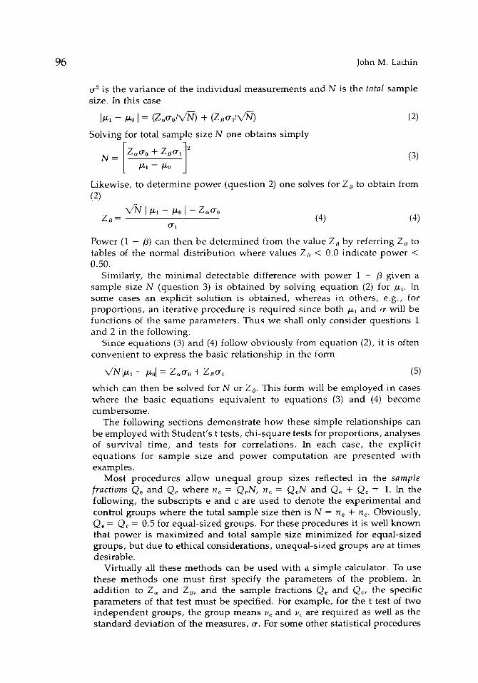
F i g u r e I The distribution of a statistic X with variance ~2 under the null hypothesis H0: /~ = /~0, i.e., the curve P(XIH0), and that under the alternative hypothesis Hi: /~ = ~1 or the curve P(XIHI), and the probabilities of Type I error (c~) and Type II error (/3), where X~ = /~0 + Z ~ .

of the ind iv idua l obse rva t ions and the sample size N. 1 G iven these distri- bu t ions one can then d e t e r m i n e c¢ and fl as s h o w n in Figure 1.

In a clinical trial the p a r a m e t e r /~ is the t rea tment -cont ro l difference in the ou tcome m e a s u r e of interest , e.g., the m e a n difference on some meas- urable pha rmaco log ic effect such as se rum cholesterol, or the difference in the p ropo r t i on d i sp lay ing an event such as heal ing. In such cases /~0 is usual ly zero and / z l is specif ied as the min ima l clinically re levant therapeut ic difference. (For a more basic in t roduc t ion to these concepts , see [2-4]).

W h e n the statistical test is conduc ted , the p robab i l i t y of T y p e I error, c~, is specif ied b y the inves t iga tor . H o w e v e r , the p robab i l i ty that a s ignif icant result will be ob ta ined if a real dif ference (/~1) exists (i.e., the p o w e r of the test, 1 - /3) d e p e n d s largely on the total s ample size N. As one increases N the sp read of the d i s t r ibu t ions in Figure I decreases , i .e. , the curves t ighten; thus /3 decreases (power increases). Thus if the statistical test fails to reach significance, the p o w e r of the test becomes a critical factor in reaching an inference. It is not wide ly apprec ia ted that the fai lure to achieve statistical s ignif icance m a y often be related more to the low p o w e r of the trial than to an actual lack of difference b e t w e e n the compe t ing therapies . Clinical trials wi th i nadequa t e s ample size are thus d o o m e d to fai lure before they beg in and serve only to confuse the issue of de t e rmin ing the mos t effective the rapy for a g iven condi t ion. Thus one should take s teps to ensure that the p o w e r of the clinical trial is sufficient to just ify the effort involved.

Converse ly , if the p o w e r of the trial in detect ing a specif ied clinically re levant di f ference (/~1) is sufficiently h igh , say 0.95, failure to achieve significance m a y p rope r ly be in te rp re ted as p r o b a b l y indica t ing negl igible r e l evan t d i f fe rence b e t w e e n the c o m p e t i n g therap ies . Thus the p r o p e r in te rpre ta t ion of a " n e g a t i v e " result is ba sed largely u p o n a cons idera t ion of the p o w e r of the exper iment .

~The n o t a t i o n N ( ~ , X2) d e n o t e s t he n o r m a l d i s t r i b u t i o n w i t h m e a n ~ a n d v a r i a n c e ~;~. If X N(p., ~2) t h e n Z = (X - p.)~-~ is d i s t r i b u t e d as N(0, 1), t he l a t t e r b e i n g w i d e l y t a b u l a t e d as

the s t a n d a r d n o r m a l d i s t r i b u t i o n .

Sample Size Determination 95

These poin ts have been i l lustrated by Freiman et al. [5] w h o showed that of 71 recent clinical trials that reached a negat ive result, 67 had p o w er less than 0.90 in detect ing a modera te (25%) therapeut ic improvement . Their conclusion is that m a n y of the therapies s tudied were not g iven a fair test s imply due to inadequa te sample sizes and, thus, inadequa te power .

S A M P L E S I Z E A N D P O W E R

The p rob lem in p lann ing a clinical trial is to de te rmine the sample size N requ i red such that in testing H0 with stated probabi l i ty of Ty p e I error ~, the probabi l i ty of Type II error is a desired small level/3. The parameters of the p rob lem are ~, iS,/~0,/~1, ]~02, and ~ .

Since the variances 22 are funct ions of N, the sample size requ i red is that which s imul taneous ly satisfies the equali t ies Pr(Z > Z~) = c¢ if H0 is true and Pr(Z > Z~) = 1 - /3 if H1 is true; where Z~ is the staildard normal devia te at the o~ significance level (e.g., Z~ = 1.645 for ~ = 0.05, one-sided) and where Z = (X - ~0)2 -1 is the s imple statistic one would use in testing Ho; where Z - N(0, 1) if H0 is t rue (see footnote 1).

It can easily be s h o w n , however , that the sample size that satisfies these equali t ies also satisfies the equali ty

I~, - ~01 = z~:~0 + z ~ : ~ , (1)

The term Z~/2 is employed for a two-tai led test. Derivat ions for part icular cases are g iven in Snedecor and Cochran [6, p. 111] and Fleiss [ 7, p. 29], among others.

This basic re la t ionship can readily be grasped from Figure 1. To relate equa t ion (1) to Figure 1, note that the critical value of X at the o~ level of significance is X~ = /z0 + Z ~ 0 . On e can thus readily der ive equa t ion (1) f rom Figure 1 where the "d i s t ance" ]/~ - ~01 is the sum of two parts , ~K~ - /~0] = Z~]~0 and ]~1 - X~I = Za~,, where Z~ results f rom the specification X~, /~1, and ~1.

This equa t ion can then be used to evaluate sample size or p o w er for the most commonly used statistical tests once ~0, ~1, and c~ have been specified. The three basic ques t ions one can ask are

1. What sample size is requi red to ensure power 1 - / 3 of detect ing a relevant d i f f e r ence /~?

2. What is the power (Z~) of the exper iment in detect ing a relevant difference k~ w h e n a specific sample size N is employed?

3. What difference i~ can be detected wi th power 1 - / ~ if the exper iment is conduc ted wi th a specified sample size N?

Usually, ques t ion 1 is employed in p lanning an exper iment and ques t ion 2 is employed in evaluat ing the results of an exper iment . Ques t ion 3 can be employed in e i ther case.

For the de te rmina t ion of sample size (quest ion 1) one s imply solves equa t ion (1) for N once the expression for the variances Xz have been obtained. In m a n y cases, ~z will be a funct ion of the form ~2 = o.Z/N, where

96 John M. Lachin

o -2 is the var iance of the ind iv idua l m e a s u r e m e n t s and N is the total sample size. In this case

IId~l - - ['~0 I = (Z~o'olX/N) + (Zao-,Ix/N) (2)

Solving for total sample size N one obta ins s imply

N= [Z,~o'o + Z~o',12 [ ~-~---~0 J (3)

Likewise , to de t e rmine p o w e r (quest ion 2) one solves for Z~ to obta in f rom (2)

X / ~ I/Xl - /Xo t - Z~o-0 Z~ = (4) (4)

o-1

Power (1 - /3) can then be de t e rmined f rom the value Z , b y referr ing Z , to tables of the normal d i s t r ibu t ion where values Z~ < 0.0 indicate p o w e r < 0.50.

Similarly, the m i n i m a l detectable difference wi th p o w e r 1 - ]3 g iven a sample size N (quest ion 3) is ob ta ined b y solving equa t ion (2) for /~,. In some cases an explicit solut ion is ob ta ined , whereas in others , e.g., for p ropor t ions , an i terat ive p rocedure is requi red since bo th ~, and o- will be funct ions of the same paramete rs . Thus we shall only consider ques t ions 1 and 2 in the following.

Since equat ions (3) and (4) follow obvious ly f rom equa t ion (2), it is often conven ien t to express the basic re la t ionship in the fo rm

- = zoo -0 ÷ z o-, (5)

which can then be solved for N or Za. This form wil l be employed in cases where the basic equations equivalent to equations (3) and (4) become cumbersome.

The following sections demonstrate how these simple relationships can be employed with Student's t tests, chi-square tests for proportions, analyses of survival time, and tests for correlations. In each case, the explicit equations for sample size and power computation are presented wi th examples.

Most procedures allow unequal group sizes reflected in the sample fractions Qe and Qc where n e = QeN, nc = QcN and Qe ÷ Q¢ = 1. In the fol lowing, the subscr ip ts e and c are used to deno te the exper imenta l and control g roups where the total sample size then is N = n e -I- no. Obvious ly , Qe = Qc = 0.5 for equal -s ized groups . For these procedures it is well k n o w n that p o w e r is m a x i m i z e d and total sample size m i n i m i z e d for equal -s ized groups , but due to ethical cons idera t ions , unequa l - s i zed g roups are at t imes desirable.

Virtually all these m e t hods can be used wi th a s imple calculator. To use these me t hods one m u s t first specify the pa ramete r s of the p rob lem. In addi t ion to Z~ and Z~, and the sample fractions Qe and Qc, the specific pa rame te r s of that test m u s t be specified. For example , for the t test of two i n d e p e n d e n t g roups , the g roup means ve and vc are requi red as well as the s tandard dev ia t ion of the measures , o-. For some other statistical p rocedures


a separate standard deviation is not required since the variance will be a function of the expectation and/or the sample size alone.

ADDITIONAL CONSIDERATIONS

Sample size evaluation for a clinical trial is almost always a matter of compromise between the available resources and the various objectives, such as safety with small effects desirable and efficacy with large effects desirable, [1, 2]. This leads to a recursive process whereby one cycles through various specifications of the desired detectable effects and considers the resulting sample size in relation to the objectives and the resources available. Eventually one reaches a sample size and statement of objectives that are consistent with each other and the available resources.

In this process, however, attention should also be given to the operational aspects of the trial. Foremost among these are the factors related to the administration of the program of therapy and the evaluation of outcome. As a simple example, consider a clinical trial of an ulcer healing agent with healing assessed endoscopically after 4 weeks. Noncompliance, dropouts, and lack of control of other factors such as diet, drinking, and smoking may all combine to reduce the observed healing rate and thus reduce the statistical power of the trial. Likewise, failure to set uniform standards for endoscopic examination and criteria for healing will increase the variability of the outcome measurement, again leading to reduced power.

Among these, a major consideration is the rate of dropouts, patients who terminate therapy for reasons related neither to the disease under treatment nor the therapy. If an R dropout rate is expected, a simple but adequate adjustment is provided by Nd = N / ( 1 - R) 2 where N is the sample size calculated assuming no dropouts and Nd that required with dropouts [1]. Likewise, to evaluate power one would use equations and tables with N = Nd(1 -- R) 2 where Nd is the observed or expected sample size. Additional procedures are described in [8] and [9].

STUDENT'S t TEST

In its most general form, Student's t is used to test the hypothesis that the mean of a normal variable, v, equals some specified value H0:/~0 = ~0 against some alternative H i : / ~ = vi, Vl ~ v0, when the variance is unknown. The test statistic is of the form t = V ' N ( x - I~o)/S where x is the sample mean with standard error S2/N, S 2 being the unbiased sample estimate of the variance o -2 on N - 1 degrees of freedom (df). The distribution of t becomes increasingly close to that of a standard normal variable as df increases, at least 30 df being required for the approximation to be adequate [10]. Thus equations (1) through (4) can be employed to yield an approximate evaluation of sample size and power.

This approach, however, will tend to overestimate power for given S 2 and N, and thus it will tend to underestimate the required sample size, although this effect is increasingly negligible for increasing df. An adequate adjustment is obtained by the correction factor f = (df + 3)/(df + 1), where

98 John M. Lachin

fN patients are actually employed after N is obtained from equat ion (3), or, alternately, by N/f used in equat ion (4) when solving for power [6, p. 114].

For those who desire an exact solution, an iterative procedure is required and is described, with brief tables, in Cochran and Cox [11, p. 19]. Under this procedure, one obtains a trial value for N that is then adjusted in light of the resulting degrees of freedom.

In sample size or power evaluation for the t test a critical feature is the specification of 0-2. For the other tests considered later (proport ions, etc.) the variances are not specified separately. Usually a value for 0-2 can be specified based on prior experiments us ing the same measurements ; in these cases it is best to use the largest value 0-2 expected. Often a pilot s tudy is helpful to provide an estimate of 0-" under the condit ions to be used in the experiment to be conducted. Of course, if power is to be evaluated after an experiment was conducted with a given N, then the obtained estimate S 2 of the variance should be employed.

A Single Mean The most basic form of the t test is the test of H0:/x0 = ~'0 for some a priori specified mean value v0 with variance 0-~, against an alternative H,: /~1 = / d l

=~ 1,0 with variance o-2. The test statistic is as presented where x is the mean of a single sample of observat ions with sample variance S 2. Given specified ~, fl, /~0, /xl, 0-0, and 0-1, the equat ions for sample size N or power (Z~) are exactly as presented in equat ions (3) and (4), respectively.

Two Independent Groups The t test is most widely used to test the null hypothes is that the means of two independen t groups are equal, H0 :~0 -- (re - vc) = 0, based on two separate samples of sizes ne = Q ~ / and n~. = Qd~/, Q,. + Qc = 1. The fractions Qe and Qc are the sample fractions and refer s imply to the propor t ion of patients in each group, N being the total sample size. The test statistic employs the pooled estimate S 2 of the common variance o-~ = o-2 = 0 -2 with N - 2 dr. It is well known that power is maximized for Q~ = Qc = 0.5.

U n d e r H, , /~, is specified as the min imal re levant difference to be detected, /~, = lye - Vc[ ¢ 0, and it follows that E0 2 = E~ = 0-2(Qe' + Q~')/N. Using equat ion (1) the equat ions for total N and Za are

0-2(Q e ' + Q¢') (z~ + Z~) 2 N = (6)

Za = V' -~ (7) 0- Q~ + Q ; '

where for equal sample sizes (Q~-I + Q~-I) = 4.0. For example, consider an experiment where o- is known not to exceed or

known to be o- = 1.0 and it is desired to detect a difference/~1 = (re - re) = 0.20. From equa t ion (6), to ensure a 90% chance of detect ing this difference (Z~ = 1.282) with c~ = 0.05 (one-sided, Z~ = 1.645), N = 858 is


requi red . This wou ld yield a t test on 856 (N - 2) df, and thus wi th the correct ion factor f = 1.006, the final sample size des i red is fN = 860.

Suppose , howeve r , that the expe r imen t was actually conduc ted wi th only 102 pat ients . The correct ion factor is 1.02 and equa t ion (7) is emp loyed wi th N = (102/f) = 100, to yield Z~ = -0 .645 , thus indica t ing that for N = 100 the expe r imen t h a d abou t 26% power . If the exper imen t p roduced a nega t ive result , howeve r , equa t ion (6) could also be used to s h o w that wi th N = 100 there was a lmost 100% p o w e r in detect ing a difference/~, = 1.0 (Za = 3.355). Thus one could safely rule out a difference on the order of /~, = 1.0.

Paired Observations In the event that the observa t ions in the two g roups are l inked together by pa i r ing or repea ted measu re s at t imes a and b on the same pat ient , the t test is conduc ted us ing the m e a n difference d = Xb - X~ wi th a s t andard error ~2 = cr~dN where o '~= 20~(1 - p) if c ry= o-~ = o -~, p be ing the p repos t correlation. From equa t ion (1) the equa t ions for N and Za for detect ing a t rue d i f fe rence /z l = Vb -- Va are:

(Z + m - (8)

Z~ = (9) Or d

which are equ iva len t to us ing equat ions (3) and (4) wi th o-,~ in place of o-0 a n d o-~.

In this ins tance, often an es t imate of o'2 is avai lable f rom pr ior experience. If not , an es t imate of cr 2 can be used wi th an es t imate of the correlat ion p. No te that pa i r ing is only efficient if p > 0, i .e. , there is pos i t ive correlat ion b e t w e e n the a and b m eas u rem en t s . If no es t imate of p is available, it is safest to a s s um e p = 0 or, nominal ly , p = 0.10.

Two Independent Groups with Paired Observations A c o m m o n related des ign is to emp loy two t rea tments in samples of sizes ne and nc where each pa t i en t also serves as his o w n control wi th measures at t imes a and b such as before and after t reatment . In this case the test statist ic is the same as for two i n d e p e n d e n t g roups where the p repos t differe_nces for eada pa t i en t are used as the ind iv idua l observa t ions ; i .e. , Xe = de and X~e = de; and where the pooled esldmate of the var iance of the d i f fe rences (S~) is e m p l o y e d . The p r o b l e m is f o r m u l a t e d as /xl = I ~ e - 3c I, 8e = (Veb -- V~) , 3c = (Vc, -- Vc~), with y2 = o.~(Q-d~ + Q~ ' ) /N . This yields equa t ions equ iva len t to equat ions (6) and (7) wi th Cro subs t i tu ted for or.

PROPORTIONS In expe r imen t s whe re the basic ou tcome is a qual i ta t ive var iable , such as success versus failure, the data are usual ly expressed as a p ropor t ion , e.g., the p r o p o r t i o n of successes, or s imp ly p. The exact p robab i l i ty d is t r ibu t ion

100 John M. Lachin

of such a p r o p o r t i o n is the b i n o m i a l d i s t r i b u t i o n tha t ha s p a r a m e t e r s N ( s a m p l e size) a n d ~r ( the t rue p o p u l a t i o n p r o p o r t i o n ) . For la rge N (i .e. , a symp to t i c a l l y ) the b i n o m i a l d i s t r i b u t i o n m a y b e a p p r o x i m a t e d b y a n o r m a l d i s t r i b u t i o n w i t h m e a n /z = ~r a n d v a r i a n c e ~ = ~r(1 - ~r)/N. T h u s , in e x p e r i m e n t s i n v o l v i n g tes ts for p r o p o r t i o n s , the bas i c e q u a t i o n s m a y be u s e d for the d e t e r m i n a t i o n of s a m p l e s ize a n d p o w e r .

A Single Proportion

In o n e - s a m p l e p r o b l e m s tha t y ie ld a s ing le p r o p o r t i o n , the h y p o t h e s i s Ho:/~0 = ~'0 is t es ted w h e r e o n e w i s h e s to de tec t a cl inical ly r e l evan t a l t e r n a t i v e H~:~I = 7r1 w h e r e 7rl > Tr0 or ~-~ < ~r0. G i v e n a p r o p o r t i o n p f r o m a s a m p l e of s ize N, the test s ta t i s t ic e m p l o y e d is Z = (p - ~r0)/E0 w h e r e E~ = ~r0(1 - 1ro)/N a n d w h e r e Z - N(0 , 1) if H0 is t rue . As an e x a m p l e , in a cohor t fo l low- u p s tudy , one m i g h t test tha t the k y e a r m o r t a l i t y equa l s tha t o b t a i n e d in a p r e v i o u s ( and c o m p a r a b l e ) cohor t , w h e r e 7r0 is tha t o b s e r v e d in this la t ter cohor t .

For the d e t e r m i n a t i o n of s a m p l e s ize or p o w e r one s u b s t i t u t e s o-2 = fro(1 - 7r0) a n d o-2 = ~1(1 - ¢rl) in to e q u a t i o n (3) or (4); the e q u a t i o n s for s a m p l e s ize N a n d p o w e r Z~ b e i n g

Z . ~ / ~ o (1 - ~'o) + Z , ,~ /~ ' , (1 - ~-1).] ~ N = - - J (10)

7r 1 7]" 0

- I - z x/;,o ( 1 - = (11)

Z~ X/~r~ (1 - ~r~)

Two Independent Proportions

In the case of t w o i n d e p e n d e n t s a m p l e s of s izes ne a n d no, the nul l h y p o t h e s i s H0:/~0 = (~'e - ~r¢) = 0 is t e s t ed w i t h the s ta t i s t ic Z = (pe - p~)/S w h e r e Pe a n d Pc are the p r o p o r t i o n s of e v e n t s in the two s a m p l e s , tr0 ~ is e s t i m a t e d as S 2 = (n~ -1 + nc l )p(1 - P), P = Q e p ~ + Qe pc, a n d w h e r e u n d e r H0, Z - N(0, 1).

For the d e t e r m i n a t i o n of s a m p l e s ize a n d p o w e r , the m i n i m a l r e l evan t difference/.~1 = Iwe - ¢rc I is t h e n spec i f ied . S ince the v a r i a n c e wil l d e p e n d on the va lue s spec i f i ed a n d no t o n the a b s o l u t e d i f fe rence , b o t h 7re a n d ~r~ m u s t b e speci f ied . Th i s y i e lds o-~ = ['/re( L - "/re) Q e 1 +_Vc(1 - rrc) Q ~ - q - U n d e r the nul l h y p o t h e s i s H0:zr~ = zr¢ = It, ~0 = 0 a_nd zr i s spec i f i ed as rr = Qezre + Qczrc. Th is t h e n y i e lds o'~ = (Q;~ + Q-~)~r (1 - rr). S u b s t i t u t i n g in to e q u a t i o n (5) y i e lds the w e l l - k n o w n f o r m u l a

X/~l~re - 1rcl = Z~X/~(1 - ~ ) ( Q e ~ + Q~-')

+ ZaX/rre(1 -- ~r~)Qe ~ + ~rc(1 - ~rc)Q~ 1 (12)

w h i c h can t h e n b e so lved for N or Za. Th i s e x p r e s s i o n can_ b e s__implified, h o w e v e r , b y n o t i n g tha t for equa l

s a m p l e s izes tr0 2 = 4rr (1 - rr) is a lways g rea t e r t h a n or equa l to o-2 = 2~re(1


- ~re) + 2¢rc(1 - 7rc). This then allows use of the s impler equa t ions

(Z~ + Z~)24~(1 - ~) N = (13)

_

Z~ - Z~ (14) 2x/~-(1 - W)

Ha lpe r i n (personal c o m m u n i c a t i o n to Paul Canner) has s h o w n that the a p p r o x i m a t i o n (13) will yield total s ample sizes no greater than Z~ + 2Z~Za a b o v e that ob t a ined f rom equa t ion (12); i .e. , to w i th in 5.86 uni ts for o~ = 0.05 (one-s ided) , /3 = 0.10.

In u s ing these formulas , note that ~r d e p e n d s on the actual values 7r~ and ~'c s p e c i f i e d u n d e r H 1 and not just on the re levant difference t~l = [~'e - 7rd- Also, since ~'(1 - 7r) is at a m a x i m u m for 7r = 0.50, it then follows that for fixed pos i t ive /~1, as 7re gets smaller, the requi red sample size also gets smaller and p o w e r increases a s s u m i n g 7rc < 7re). In such p rob l ems , therefore, it is safest to speci fy the largest realistic va lue for 7rc (where 7re > Tr~ and, ~-~ < 0.50) so as not to unde re s t i m a t e sample size or overes t ima te power .

For example , s u p p o s e we w i s h e d to conduct a control led clinical trial of a n e w the rapy and the rate of successes in the control g roup is not expected to be grea ter than 7rc = 0.05. Further , we would cons ider the n e w the rapy to be s u p e r i o r - - c o s t , r i s k s and other f_actors_considered--if ~r~ = 0.15, thus y ie ld ing t~l = 0.10, Ir = 0.10, and 47r(1 - 7r) = 0.36. Us ing equa t ion (13) wi th ot = 0.05 (one-s ided) and ~8 = 0.10 yields N = 310 ( rounded up f rom 308.4); the m o r e prec ise formula (12) yields N = 306 ( rounded f rom 304.6).

Suppose , howeve r , that the expe r imen t was conduc ted wi th only N = 100. Us ing equa t ion (14) indicates that the p o w e r of the expe r imen t in d e t e c t i n g / ~ = 0.10 wi th 7rc = 0.05 is only 51% (Z~ = 0.022). If a nega t ive result was ob ta ined , howeve r , one m i g h t wish to d e t e r m i n e the p o w e r of h a v i n g detec ted larger differences, s a y / ~ = 0.40 for 7re = 0.05. This yields Tre = 0.45, ¢r = 0.25, and 2X/~'(1 - ~) = 0.886. From equa t ion (14) we find that N = 100 yields 99.9% p o w e r (Z a = 2.87). Thus a t rue difference of this m a g n i t u d e could conf ident ly be ruled out.

For fu r the r i l lus t ra t ion, Lachin [2] u sed these p rocedures to discuss s amp le size cons idera t ions for FDA Phase II and III clinical trials of n e w drugs , and these m e t h o d s have been used in a var ie ty of clinical trials. Addi t ional references include [1, 5, 7, and 8].

T h e A n g u l a r T r a n s f o r m a t i o n

The p r o c e d u r e s jus t desc r ibed are usua l ly p re fe r red s ince the tests for p ropo r t i ons us ing the normal app ro x ima t ion to the b inomia l are equiva len t to the usual X 2 tests (see u n d e r Discuss ion following). Others [12], howeve r , have e m p l o y e d the angu la r t r ans format ion A(p) = 2 arcsin V ~ , whe re A(p) is expressed in rad ians , no t degrees. 2 G iven a p ropo r t i on p wi th b inomia l

2For those w h o s e calculators p rov ide the s in func t ion in degrees , the convers ion factor is arcsin (radians) = (0.017453) arcsin (degrees).

102 John M. Lachin

expecta t ion 7r, then A(p) is app rox ima te ly normal ly d i s t r ibu ted as N[A(rr), N-l ] . Since the var iance (~2 = 1/N) is n o w i n d e p e n d e n t of the expecta t ion, the resul t ing sample size and p o w e r equa t ions are fur ther simplif ied. This approach , howeve r , is not as accurate as that descr ibed herein.

As an i l lustrat ion, aga in cons ider the example p resen ted earlier unde r Two I n d e p e n d e n t P ropor t ions wi th 7r¢ = 0.05 and 7re = 0.15. The equa t ion ba sed on the arcsin t r ans fo rmat ion wi th equal sample sizes is

N = 2(Z~ + Z~) 2 [A(cre) - A(cr~)] 2 (15)

and for c~ = 0.05 (one-s ided) and /~ = 0.10 we find N = 290. This is s o m e w h a t less than the N = 310 es t imated f rom the app rox ima te equa t ion (13) and the more precise formula (12), which yields N = 306. In general the angula r t r ans fo rmat ion p rocedure yields N abou t 3 - 5 % less than that f rom equa t ion (12), wi th ~ = 0.05 (one-s ided) , fl = 0.10.

Paired Observat ions

N o w consider the p r o b l e m whe re two g roups of obse rva t ions are l inked toge ther in some w a y such as th rough ma tch ing or repea ted measures on the s a m e ind iv idua l s at t imes a and b. This is exactly ana logous to the p r o b l e m of the t test for pa i red obse rva t ions except that the ou tcome is n o w qual i ta t ive ra ther than quant i ta t ive . In this case, the basic data are expressed a s

Time a

Time b +

m++ [ m .

m ÷ m _

mr,

where m+_, for example , is the n u m b e r of pairs wi th (+) for observa t ion a ( t ime a or the a pa i r m e m b e r ) and ( - ) for o b s e r v a t i o n b. For the a obse rva t ions rn~ is the total n u m b e r (+) and l ikewise mb for the b observa- t ions. The f requenc ies (re's) are then conver ted to p ropor t ions (p's) by d iv id ing b y the total n u m b e r of pairs , N.

In such p rob l ems , one wishes to test the null hypo thes i s H0:/~0 = (Trb - 7ra) = 0. Note , howeve r , that Trb -- 7ra = 7r_+ -- 7r+_; thus the p r o b l e m can then be expressed solely in te rms of the d iscordant p ropor t ions 7r_+ and 7r+_ whe re H0 impl ies that 7r_+_= 7r_+_ = Tr. The test statistic e m p l o y e d is Z = ~__+ - p+_)/S where S 2 = 2p/N, p = 1/2(p_+ + p+_) is the sample es t imate of Tr and whe re u n d e r H0, Z - N(0, 1). Note that Z 2 is equ iva len t to the McNem ar X 2 statistic usual ly e m p l o y e d (see u n d e r Discuss ion following).

For s ample size or p o w e r de t e rmina t ion the clinically re levant difference /xl = 17r-+ - 7r+_] is specified. The co r re spond ing var iance has been s h o w n b y Mie t t inen [13] to be o'21 = 2rr_+ 7r+_/~" whe re ~ = V2(Tr_+ + 7r+_). Unde r

Sample Size Determinat ion 103

H0:/-~0 = (Tr_+ - It+_) = 0, w h i c h i m p l i e s o-02 = 2Ir. S u b s t i t u t i n g i n t o e q u a t i o n (5) y i e l d s t h e b a s i c r e l a t i o n s h i p

V ~ ] ~ _ + - ~r+_ I = Z ~ V ' ~ + Z~X/2~_+ ~r+_/~ (16)

w h i c h can b e s o l v e d for t he to ta l n u m b e r of p a i r e d o b s e r v a t i o n s (N) or p o w e r ( f rom Z~).

For e x a m p l e , c o n s i d e r tha t w e w i s h to d e t e c t a d i f f e r e n c e / ~ , = 0.15 w h e r e ~+_ = 0.05, ( i m p l y i n g ~-_+ = 0.20), u s i n g e q u a t i o n (16) for a = 0.05 (one- s i d e d ) , / 3 = 0.10 y i e l d s N = 80.

Two Independent Groups with Paired Observations A s w i t h t he t t e s t , t h i s can b e e x p a n d e d to t h e p r o b l e m of t w o i n d e p e n d e n t g r o u p s of p a t i e n t s w i t h p a i r e d o b s e r v a t i o n s on each p a t i e n t . 3 U n d e r th i s d e s i g n , r e p e a t e d o b s e r v a t i o n s ( + or - ) a r e o b t a i n e d at t i m e s a a n d b o n t w o i n d e p e n d e n t g r o u p s of s i z e s ne = QeN a n d nc = QcN. The nul l h y p o t h e s i s of n o t r e a t m e n t b y t i m e i n t e r a c t i o n H0:/~0 = 8e - 8c = 0 is to b e t e s t e d , w h e r e 8e = ~eb - 7tea is t h e c h a n g e o v e r t i m e in t h e t r e a t e d g r o u p a n d 6c = •rcb - Irca is t h a t for con t ro l s .

A s s h o w n u n d e r P a i r e d O b s e r v a t i o n s , t h e p r o b l e m can b e e x p r e s s e d so l e ly in t e r m s of t h e d i s c o r d a n t o b s e r v a t i o n s w i t h i n t h e t w o - w a y t ab le for each g r o u p , d e n o t e d as ~'e+-, ~re-+, rrc+_, a n d ~'c-+, w h i c h i n t u r n d e f i n e t he d e g r e e of i n t e r a c t i o n /-~1 = 1Be - 6cl to b e d e t e c t e d . U n d e r H1 the s a m p l e s t a t i s t i c D = de - dc = Pc-+ -- Pe+- -- Pc-+ + Pc+- is n o r m a l l y d i s t r i b u t e d w i th /~1 = IAI w h e r e

A = ~e-+ -- ~e+- - Ire_+ +I rc+_ (17)

a n d

o_2 = 4~re-+Tre+_ 41rc_+ Ire+_ (18)

Q e(~-e-+ + 1re+-) + Qc(1rc-+ + ~'c+-)

A su f f i c i en t c o n d i t i o n for H0 to b e t rue is t h e a s s u m p t i o n of h o m o g e n e i t y w h e r e i n t he t r e a t e d a n d con t ro l g r o u p s a r e a s s u m e d to b e d r a w n f r o m the s_ame p o p u l a t i o n w i t h c o m m o n p a r a m e t e r s or+_ = Qerre+- + Q j r c + - a n d

~r_+ = Qelre_+ + Q j r c - + y i e l d i n g /~0 = 0. A l t e r n a t i v e l y , such a s e v e r e a s s u m p t i o n m a y n o t b e r e q u i r e d a n d o n e m i g h t fit a n o - i n t e r a c t i o n m o d e l to t h e i n t e r a c t i o n p a r a m e t e r s to o b t a i n t h e se t of n o - i n t e r a c t i o n p a r a m e t e r s ,

~-', as 7re+_ = rre+_ + T, Ire-+ = ~re-+ - T, ~rc+- = 7re+_ - T a n d ~c-+' = Ire_+ + T, w h e r e T = A/4 a n d A is d e f i n e d as in e q u a t i o n (17). A l t e r n a t i v e l y , o n e m i g h t e m p l o y t h e s a m e p a r a m e t e r s ~'c+-, rre+_ u n d e r H0 a n d H , a n d t h e n c o m p l e t e t h e n o - i n t e r a c t i o n m o d e l w i t h p a r a m e t e r s ~-~+_ = 1re+_, 7r~_+ = 7re_+ + 1/2A, Ir~+_ = Ire+_ and 7r'_+ = 7r~_+ - I/2A. In each case'D is normally distributed with/~0 = 0 and variance o-2 of the same form as equation (18) but with ~r' substituted for the ~.

3Lachin et al. [1] also present extensions to analyses across independent subgroups within two independent primary groups.

104 John M. Lachin

The null hypothes i s H0:A -- 0 is then tested using Z = (de - de)/3-o, usually with 3-0 defined from the s a m p l e p ' s under the assumpt ion of homogenei ty.

r r ! t In the latter case 77e+- = 77¢+- = rr÷_ and 77e + : 77e + : 77_+. Subst i tut ing into equat ion (5) yields the equat ion

7 7 e + - - + 77c+ I =

Z~ ~ Q 4rr;_+77'~+_ (77;-+ + 77;÷_)

+ Z , x / 47r~. + 7 r e + _

Qe (Tr~_+ + ~re+ )

4 ¢ ' "w e 4 . T T e + _ + Q(. (77[. + + 7re+ )

4 q T c + 77c+-~ + Q¢(77e + + 77c+-)

(19)

with the ~-' defined under the assumpt ion of homogene i ty or after fitting one of the no- interact ion models. This can then be solved for total sample size N or power .

For example, consider a clinical trial in which 100 patients, 50 in each group, are to unde rgo evaluat ion before and after t reatment and we desire the power of the s tudy to detect group differences. The parameters of the problem may be specified as 77~.+ , 8~, (which yields 77e-+), rre+-, and A (which then yields 77e-*). Assume we are interested in detecting moderate differences such as 77~+_ = 0.03, 3,. = 0.05, 77e+- = 0.03, and/x l = A = 0.15. Using ' and ' = rr~.+_~ = 77e+- %+_ rre, , fitting a no-interact ion model and then us ing equa t ion (19) with c~ = 0.05, (one-sided), we find that Zs -- 0.734 and power = 77% (fl = 0.23). Solving for sample size in equat ion (19) with fl = 0.10 indicates that N = 151 yields 90% power of detecting these same effects.

D i s c u s s i o n

Although the problems just given are presented in terms of the normal approximat ion to the binomial , a two-tailed test us ing each of the statistics, Z, presented under A Single Proport ion, Two Independen t Proport ions , and Paired Observat ions yields the same p value as the one df chi-square test usually employed in the same situation. For each of these Z and chi-square (X 2) tests, it is easily shown that X 2 = Z 2 and thus that the p values for the two tests are the same. For example, the 1 df chi-square critical value at the 0.05 level is X~.05 = 3.841, which equals (1.96) 2, where Z0.02~ = 1.96 (the two- tailed critical value at the 0.05 level). Thus, if one in tends to use the inheren t ly two-ta i led ch i -square test, two-ta i led sample size or power de terminat ion should be employed (i.e., us ing Z~/2 rather than Z~). Other- wise, sample size may be severely underes t imated.

When a two-tai led test is to be conducted, however , one mus t carefully consider each of the two possible alternatives. For example, in tests of a single propor t ion , H0:77 = 77o is tested against an alternative, which for a two-s ided test is specified a s H 1 : ~ 1 = 3 = I'a-1 - 770[ ~ 0. The two-s ided test thus implies two alternative values for 771:771u = 77o + 3 and 771e = 77o - 3. Obviously, since the variances depend on 7rl, the est imated sample size will be greater, and power smaller, for the alternative (77~u or 77~e) closest to 0.50. fNote that ~-(1 - w) is maximized at 7r = 0.50]. In fact, the larger of the two resulting sample size estimates may be as much as 4.64 times the smaller


est imate . Thus , if a two- ta i led analysis is to be conducted , one should cons ider the two impl i ed a l ternat ives (e.g., rri~ and 7r~e) and use whichever is closest to 0.50.

An a l ternat ive would be to employ sample size p rocedures us ing the p o w e r funct ion of the ch i -square test itself, which is inheren t ly two-tai led. Lachin [14] d iscusses this p rocedu re for the general r x c cont ingency table and s h o w e d that the use of the l imit ing chi -square p o w e r approach and the two-ta i led a sympto t i c normal equa t ion (11) were in close ag reemen t for the 2 x 2 con t ingency table.

SURVIVAL ANALYSIS

In m a n y clinical trials, s imple p ropor t ions as descr ibed in the last section will be used to evaluate the ou tcome, such as to evaluate the heal ing or i m p r o v e m e n t rate in an acute condi t ion wi th a shor t - t e rm therapy. In m a n y other cases, howeve r , the impor t an t feature is not only the ou tcome event , such as death , bu t the t ime to the terminal event , the surv ival time. In these trials, the data is ana lyzed us ing l ife-table me thods that consider the t ime to the terminal event for each pa t ien t and that p rov ide a more power fu l e s t ima te of the, say, T year surv iva l than is o b t a i n e d f rom the crude p ropo r t i on of surv ivors after T years. Some basic references on this procedure are [15-17].

The basic l i fe- table m e t h o d of analysis is d i s t r ibu t ion free in that no unde r ly ing a s s u m p t i o n s abou t the d is t r ibu t ion of t ime to event need be specified. For s ample size evaluat ion, howeve r , some such a s s u m p t i o n m u s t be made . The mos t c o m m o n a s s u m p t i o n is that t ime to survival is exponen- tially d i s t r ibu ted wi th haza rd rate h, where at any t ime t the p ropor t ion of surv ivors , P~(t), is g iven as Pdt) = e -~t. Unde r this model log [Ps(t)] is l inear ly decreas ing in t ime wi th slope ~. In a cohort of N pat ients , all fo l lowed to the terminal event wi th m e a n survival t ime M, the haza rd rate is es t imated as L = M -~ and asymptot ica l ly L ~ N(h , h2/N), [18].

Two Independent Groups

Cons ide r that there are two i n d e p e n d e n t g roups of sizes ne and nc all fo l lowed to the terminal event where t ime t is measu red f rom the t ime of en t ry in to the study. The null hypo thes i s of equal i ty of survival is equ iva len t u n d e r exponent ia l surv iva l to H0: (he - he) = 0, which can be tested us ing the statistic Z = (Le - Le)/S where Le and Le are the es t imated haza rd rates, Le = M ; ' , Lc = M ~ 1, S 2 = (n ; ~ + n ~ ) L 2, L -- (QeLe + QcLc), and where u n d e r H0, Z - N(0, 1).

For the de t e rmina t ion of sample size and p o w e r one specifies the min ima l re levant difference/~1 = [he - Xd, which yields o-~ = ()~e 2 Q~-I+ k~Q~-I). U n d e r the null hypothes i s /~0 = 0 and o-02 = ~2(Q~-1 + Q~-I) where h = Qe)~e + Qehe. Subs t i tu t ing into equa t ion (5) yields

x//~lhe - he I = Z~X/x2 (Qe I + Q~I) + z a x / ) ~ Q ; ' + h ~ q ~ ~ (20)

which can then be solved for N or Z~. This equa t ion was also p re sen t ed b y Pas te rnack and Gilber t [19] and was

106 John M. Lachin

shown by George and Desu [20] to be slightly conservat ive in compar ison to the exact d is t r ibut ion of the ratio Le/L¢, which has an F dis tr ibut ion. George and Desu also present the following approximat ion

x,/Ni~/2t~n(kdhe)] = Z , + Z~ (21)

which they show to be accurate to wi th in two sample units of the exact solution.

Another approximat ion can be obta ined directly from equa t ion (20) by not ing that for equal sample sizes 4h" is always less than or equal to 2(he 2 + 2~c2). This then yields

~/Xl~-e - 2,~l/(~ ÷ 2~) = Z~ ÷ Z~ (22)

w h e n us ing equal sample sizes. This approx imat ion will yield values be tween those from equa t ion (20) and the approximat ion (21) of George and Desu and can be shown to be wi th in Z~ less than that ob ta ined from equa t ion (20).

Two Independent Groups with Censoring The formula t ion just p resen ted will rarely be applicable because it assumes that all N pat ients will be fol lowed to the terminal event no matter how much t ime is requ i red for the last pa t ient to reach that event. This is rarely practicable. A more realistic approach is to allow for the trial to be te rminated at t ime T. Assume that the pat ients enter the trial at a un i form rate over the interval 0 to T and that exponent ia l survival applies, as earlier. If we denote

d?()O = )~3T/(hT - 1 + e -v/) (23)

t h e n it can be s h o w n thato-02= (h()l)(Qel + Q;~) a n d o-12= ~()le)Qe' + q)(2~c)Q~ -1 where h = Qe2~ + Q¢)~c [18]. Subs t i tu t ing /z , = [ke -- )%[, /Z0 = 0, ¢02 , and o-12 into equa t ion (5) yields

x lxe - xc I = Z~X/q)(X)(Qe ~ + Q;1) + z~x/q~(he)Qg-~ + ~B(;%)QZ-' (24)

w i th the 6(2,) as defined in equation (23). This can then be solved for sample size N or power Z~.

These express ions can be s implif ied, however , since empir ical ly for Qe = Qe, o-21> o'~, and as employed by Gross and Clark [18, p. 264] we can use the s imple equa t ion

x/NIKe - ~.c[ = (Z~ + Z~)x/(h()~e)Qe ~ + 6(Xc)Q; 1 (25)

Again this approximat ion is h ighly accurate. In the event that all pat ients enter the trial at the same poin t , or if each

pat ient enters the trial at r andom but each is only fol lowed up to T years after entry, the resulting equat ions are identical except that (h(h) in equat ion (23) becomes s imply h2/(1 - e-at).

At' this po in t it should be no ted that the sample size ob ta ined with a


s tudy of T years dura t ion is that requi red to yield the same n u m b e r of deaths (events) as ob ta ined from equat ion (21), al lowing for the fact that not all pat ients will have d ied when the s tudy is terminated. This is also true of the fol lowing procedure .

Two Independent Groups with Limited Recruitment and Censoring In the formula t ion just presented , note that pat ients are eligible to enter the trial up to the trial end date, t ime T. Usually, however , it will be desired to recruit pat ients for s tudy over an interval 0 to To and then to follow all recrui ted pat ients to the t ime of the terminal event, or to t ime T where T > To. Based on the deve lopments in [18, pp. 66-67], it can readily be shown that the variances o-02 and 0-2 are as in the previous section bu t with q)()0 n o w defined as

e-~ (7. - T,,) _ e - ~r ] - , (26) cb*(h) = )~2 1 - hTo

I

The desi red sample size or power is ob ta ined on subs t i tu t ing 6*(k) for ~b() 0 in equa t ion (24), or in equa t ion (25) to yield an accurate approximat ion , and solving for N or Z~.

For example, consider that a clinical trial is to be conducted for a disease wi th modera te levels of mortal i ty with hazard rate ~ = 0.30, y ie ld ing 50% survivors after 2.3 years. Suppose that with t reatment we are interested in a reduct ion in hazard to ~ = 0.2, i.e., an increase in survival to 64% at 2.3 years. With equal-s ized groups , a = 0.05 (one-sided) and fl = 0.10, equa t ion (20) yields N = 218 deaths are requi red , i .e. , 218 pat ients all fol lowed to t ime of death. The approximat ion (22) yields N = 216 and the equa t ion (21) of George and Desu yields N = 210. If the s tudy was to be te rminated after 5 years, then us ing equa t ion (24) with equat ion (23) yields N = 504 patients; the approximat ion yields N = 508. Finally, assume that recru i tment was to be te rmina ted after the first 3 years of a 5-year study, then us ing equat ion (24) with equa t ion (26) yields N = 378.

Note that unde r all these plans the sample size requ i rements are based on the need to accrue approximate ly 210 deaths dur ing the study. Also note that if a fixed n u m b e r of pat ients is to be s tudied, it is bet ter for those pat ients to be recrui ted quickly and fol lowed for a longer per iod of t ime than to extend the per iod of s tudy and reduce the rate at which the pat ients enter the study. This example shows that 504 pat ients would be needed for a 5-year s tudy where the pat ients can enter the s tudy evenly dur ing the full 5-year per iod , whereas 378 pat ients would be needed if recrui tment was compressed into a 3-year per iod with total s tudy dura t ion again 5 years. The reason for this qui te s imply is related to the total pa t ien t months of exper ience of the cohort , i .e., the elapsed t ime from the t ime of randomi- za t ion to t ime T s u m m e d over all pa t ien t s . For a 5 -y ea r s t u d y wi th recru i tment compressed into the initial 3 years, the average pa t ien t months of exposure would be 3.5 years, whereas for a 5-year s tudy with recru i tment spanning the total 5 years, the average exposure to t rea tment would be 2.5 years.

108 John M. Lachin

C O R R E L A T I O N S

In obse rva t iona l s tud ies tha t i nvo lve cor re la t ions as the p r inc ipa l f o r m of ana lys i s , t wo types of h y p o t h e s e s are usua l ly tested: (1) w h e t h e r a t rue cor re la t ion ac tual ly exists u s i n g H0: p = 0 ve r sus H~: p = pl :~ 0; a n d (2) w h e t h e r t wo cor re la t ions are s ign i f ican t ly d i f fe ren t u s i n g H0: (pc - Pc) = 0 ve r sus H~: /x~ = (Po - Pc) :~ 0. T he s imples t a p p r o a c h to such p r o b l e m s is to e m p l o y F i she r ' s a rc t anh t r a n s f o r m a t i o n [5]:

C(r) = 1/2logo (1_+ r) (1 r)

G i v e n a s a m p l e corre la t ion r b a s e d on N o b s e r v a t i o n s tha t is d i s t r i bu t ed a b o u t an ac tua l co r r e l a t ion v a l u e (pa ramete r ) p, t h e n C(r ) is n o r m a l l y d i s t r i b u t e d w i t h m e a n C ( p ) a n d va r i ance o -2 = 1 / ( N - 3). The t r a n s f o r m a t i o n of r to C (and vice versa) is w i d e l y tabu la ted . (No te tha t this is usua l ly t e r m e d F i she r ' s Z t r a n s f o r m a t i o n , b u t w e he re use C to avo id conflict in no ta t ion . )

A S i n g l e C o r r e l a t i o n

In de tec t ing a re levan t s imp le cor re la t ion of deg ree Hi: /~1 = Pl, one tests the nul l h y p o t h e s i s H0: p = 0 u s i n g the test s tat is t ic Z = C(r)~ - 3 w h e r e Z

N(0, 1). S u b s t i t u t i n g in to e q u a t i o n (5) y ie lds

- 3C(pl) = Z~ + Z~ (27)

f r o m w h i c h the r e q u i r e d s amp le s ize or p o w e r m a y be ob ta ined . O b v i o u s l y , to de tec t a t rue cor re la t ion p~ g rea te r t h a n 0.50 [C(p~) = 0.549], a small N w o u l d suffice. N o t e tha t Ho: p = 0 is e q u i v a l e n t to a null h y p o t h e s i s tha t the r eg re s s ion coeff ic ient is also zero .

T w o I n d e p e n d e n t C o r r e l a t i o n s

In de tec t ing a re levan t d i f fe rence in corre la t ions Hi : /~1 = IC(po) - C(pc)l =~ 0 o b t a i n e d f r o m two i n d e p e n d e n t s a m p l e s , the null h y p o t h e s i s Ho: /z0 = 0 is t es ted u s i n g the stat ist ic Z = C(ro) - C(ro) /~o w h e r e ~ = N -1 (Qe I + Q~-I), no - 3 = Q o N , n¢ - 3 = Q c N , a n d w h e r e u n d e r H0, Z - N(0, 1). The corre la t ions ro a n d rc are o b t a i n e d f r o m t w o samples of s izes no a n d no such as r e = re(uv ) a n d r¢ = rc{uv~ for var iab les u a n d v in g r o u p s e a n d c.

Subs t i t u t i ng /xo = 0, /z, = IC(pe) - C(Po)I, and E~ = ~o z in to e q u a t i o n (5) y ie lds

X/N-IC(po) - C(pc) l = Z~ + Z~ (28)

x / Q ; ' + Q~-'

w h i c h can t h e n be so lved for total s amp le s ize (N) or p o w e r (Z~). N o t e tha t N f r o m e q u a t i o n (28) will actual ly be six un i t s less t h a n tha t actual ly n e e d e d s ince n e + n e - 6 = N.

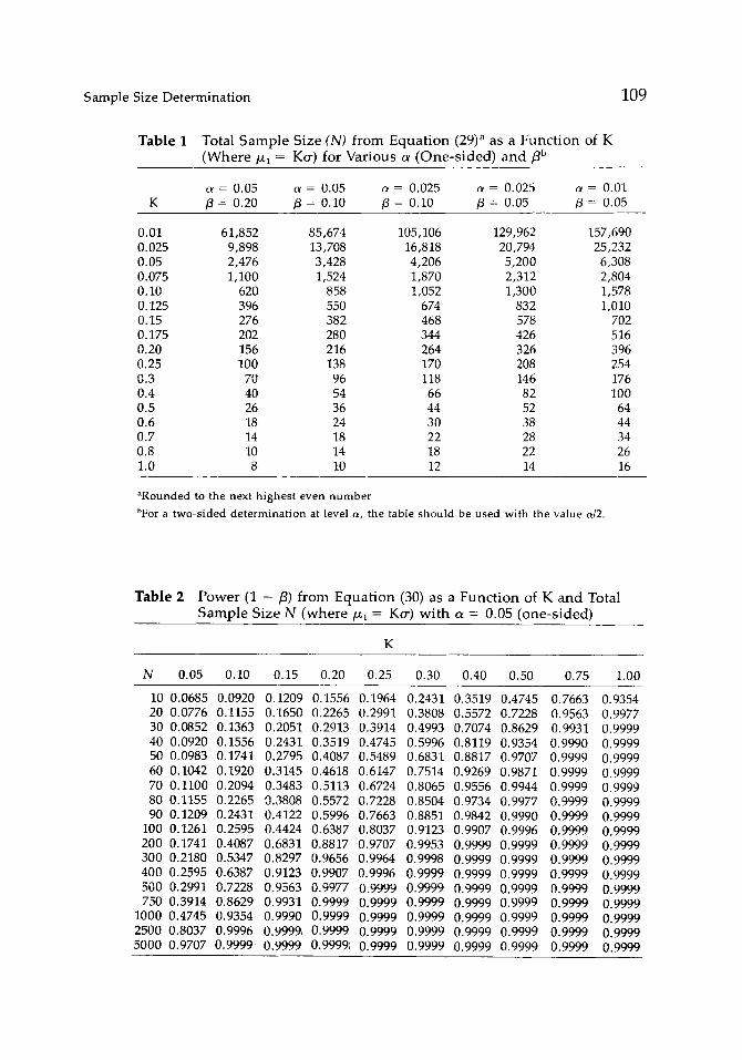
S a m p l e Size D e t e r m i n a t i o n

T a b l e I T o t a l S a m p l e S i z e (N) f r o m E q u a t i o n (29) a a s a F u n c t i o n of K ( W h e r e / z l = Kor) f o r V a r i o u s a ( O n e - s i d e d ) a n d fib

109

a = 0.05 a = 0.05 a = 0.025 a = 0.025 a = 0.01 K fl = 0.20 fl = 0.10 fl = 0.10 fl = 0.05 fl = 0.05

0.01 61,852 85,674 105,106 129,962 157,690 0.025 9,898 13,708 16,818 20,794 25,232 0.05 2,476 3,428 4,206 5,200 6,308 0.075 1,100 1,524 1,870 2,312 2,804 0.10 620 858 1,052 1,300 1,578 0.125 396 550 674 832 1,010 0.15 276 382 468 578 702 0.175 202 280 344 426 516 0.20 156 216 264 326 396 0.25 100 138 170 208 254 0.3 70 96 118 146 176 0.4 40 54 66 82 100 0.5 26 36 44 52 64 0.6 18 24 30 38 44 0.7 14 18 22 28 34 0.8 10 14 18 22 26 1.0 8 10 12 14 16

aRounded to the next highest even number

hFor a two-sided determination at level a, the table should be used with the value a/2.

T a b l e 2 P o w e r (1 - ]3) f r o m E q u a t i o n (30) a s a F u n c t i o n of K a n d T o t a l S a m p l e S i z e N ( w h e r e / z l = Ko-) w i t h a = 0 .05 ( o n e - s i d e d )

K

N 0.05 0.10 0.15 0.20 0.25 0.30 0.40 0.50 0.75 1.00

10 0.0685 0.0920 0.1209 0.1556 0.1964 0.2431 0.3519 0.4745 0.7663 0.9354 20 0.0776 0.1155 0.1650 0.2265 0.2991 0.3808 0.5572 0.7228 0.9563 0.9977 30 0.0852 0.1363 0.2051 0.2913 0.3914 0.4993 0.7074 0.8629 0.9931 0.9999 40 0.0920 0.1556 0.2431 0.3519 0.4745 0.5996 0.8119 0.9354 0.9990 0.9999 50 0.0983 0.1741 0.2795 0.4087 0.5489 0.6831 0.8817 0.9707 0.9999 0.9999 60 0.1042 0.1920 0.3145 0.4618 0.6147 0.7514 0.9269 0.9871 0.9999 0.9999 70 0.1100 0.2094 0.3483 0.5113 0.6724 0.8065 0.9556 0.9944 0.9999 0.9999 80 0.1155 0.2265 0.3808 0.5572 0.7228 0.8504 0.9734 0.9977 0.9999 0.9999 90 0.1209 0.2431 0.4122 0.5996 0.7663 0.8851 0.9842 0.9990 0.9999 0.9999

100 0.1261 0.2595 0.4424 0.6387 0.8037 0.9123 0.9907 0.9996 0.9999 0.9999 200 0.1741 0.4087 0.6831 0.8817 0.9707 0.9953 0.9999 0.9999 0.9999 0.9999 300 0.2180 0.5347 0.8297 0.9656 0.9964 0.9998 0.9999 0.9999 0.9999 0.9999 400 0.2595 0.6387 0.9123 0.9907 0.9996 0.9999 0.9999 0.9999 0.9999 0.9999 500 0.2991 0.7228 0.9563 0.9977 0.9999 0.9999 0.9999 0.9999 0.9999 0.9999 750 0.3914 0.8629 0.9931 0.9999 0.9999 0.9999 0.9999 0.9999 0.9999 0.9999

1000 0.4745 0.9354 0.9990 0.9999 0.9999 0.9999 0.9999 0.9999 0.9999 0.9999 2500 0.8037 0.9996 0.9999 0.9999 0.9999 0.9999 0.9999 0.9999 0.9999 0.9999 5000 0.9707 0.9999' 0,9999 0.9999; 0.9999 0.9999 0.9999 0.9999 0.9999 0.9999

Tab

le

3 K

V

alue

s fo

r U

se

wit

h T

able

s 1

and

2 or

E

quat

ions

(2

9)

and

(30)

a

t% U

nd

er

the

n

ull

E

qu

ati

on

Sta

tist

ica

l te

st

hy

po

the

sis

(H0

) t*

~ u

nd

er

H,

in

tex

t

K

as

a fu

nc

tio

n

of

0 =

(g

j -

/z0)

K

for

eq

ua

l sa

mp

le

siz

es

K

for

un

eq

ua

l sa

mp

les

wit

h

sam

ple

fr

ac

tio

ns

Q~

an

d

Qc

wh

ere

Q

* =

(Q

e'

+

Q;

';

t T

ests

fo

r M

ean

s

(See

Stu

den

t's

t te

st f

or

corr

ecti

on

fac

tor)

I.

A s

ing

le s

amp

le m

ean

Vo

vl

2.

Tw

o i

nd

ep

en

de

nt

(pc

- pc

) =

0 v~

-

vc

gro

up

s e

an

d c

3.

Co

rrel

ated

ob

serv

atio

ns

(vb

- %

) =

0

vb -

v~

at t

imes

a a

nd

b

4.

Tw

o in

de

pe

nd

en

t (8

~ -

6~)

=

0 (f

i e -

fi

e)

gro

up

s w

ith

pai

red

fi~

=

re0

- v

~

ob

serv

atio

ns

fie =

vC

b -

v~a

Tes

ts f

or

Pro

po

rtio

ns

1.

A s

ing

le p

rop

ort

ion

No

rmal

zr

0 zr

~ =

r%

ap

pro

xim

ati

on

An

gu

lar

A O

ro)

A ( T

r ~)

tran

sfo

rmat

ion

A(*

r) =

2

arcs

in X

/~ i

n r

adia

ns

2.

Tw

o in

de

pe

nd

en

t

gro

up

s e

and

c

No

rmal

(w

e -

we)

=

0 rr

~ -

rr c

ap

pro

xim

ati

on

An

gu

lar

[A(r

r~)

- A

(Tr~

) l =

0

A(~

) -

A (~

<,)

tran

sfo

rmat

ion

3,4

6,7

8,9

6,7

10,

11

13,1

4

15

Iv,

- vo

lta"

N.A

.

(o .2

=

var

ian

ce o

f th

e o

bse

rvat

ion

s)

Iv~

- ~,o

l/o.,~

N

.A.

((if

1 =

v

aria

nce

of

the

dif

fere

nce

s xb

-

x<D

16,

- a~

li2o'<

, la

,-

aol/o

-~x/

Q"

See

Pro

po

rtio

ns,

A S

ing

le P

rop

ort

ion

~A('r

ri)

- A(

Tro)

] N

.A.

V21z

r~ -

~rA

~(1

- ~r

)l-t

7r =

(w

~ +

~r

D/2

Vz~

4(z%

) -

A(z

r~) I

See

Pro

po

rtio

ns,

T

wo

Ind

ep

en

de

nt

Pro

po

rtio

ns

iA0,

0 -

A(~

01/x

/q;

3. Correlated o

bservations

(n_+ -

7r+_

) =

0 n_+ -

It+_

16

at t

imes a

and b

4.

Tw

o in

dep

end

ent

a~ -

ae

=

0 ae

-

ae

19

gro

up

s w

ith

pai

red

8e

= we-+ -

ere+

-

observations

8e = ~r

c_+

- we+-

Survival A

nalysis--Exponential Model

1. Two independent

groups without

censoring

Normal approximation

(Xe

- ;%) =

0 ke

- ;%

22

or

(~/;%

) =

I Xd

;%

21

2.

Tw

o in

dep

end

ent

(;% -

;%

) =

0

;% -

;%

25

gro

up

s w

ith

cen

sori

ng

at

tim

e T

23

3.

Tw

o in

dep

end

ent

(;% -

X

e) =

0

;% -

;%

25

gro

up

s w

ith

en

try

to

To

and

cen

sori

ng

at

tim

e T

>

To

Tes

ts f

or C

orr

elat

ion

s

1. A

sin

gle

co

rrel

atio

n

C(p

o)

C(p

l)

27

C(p

) =

F

ish

er's

Iz,

ansf

orm

atio

n a

nd

in

Tab

les

1 o

r 2

or

in e

qu

atio

ns

(29)

an

d (

30)

on

e u

ses

N

- 3.

2. T

wo

ind

epen

den

t [C

(p~)

-

C(p

~)]

=

0 C

(p~)

-

C(p

~)

28

gro

up

s e

and

c

See

Pro

po

rtio

ns,

Pai

red

N

.A.

Ob

serv

atio

ns

See

Pro

po

rtio

ns,

Tw

o I

nd

epen

den

t G

rou

ps

wit

h P

aire

d

Ob

serv

atio

ns

Ix.

- ~1

/(~

+ x4

[tn(

;%/~

)]/2

Ix,-

;%

112~

x~) +

2q

~(;%

)]-I

6(x) =

x~rl

(XT-l-e -x

T)

In,-

;%

112~

*(;%

) +

24*(

;%)]

-I

See

Su

rviv

al A

nal

ysi

s, T

wo

Ind

epen

den

t G

rou

ps

See

Su

rviv

M A

nal

ysi

s, T

wo

Ind

epen

den

t G

rou

psw

ith

Cen

sori

ng

See

Su

rviv

al A

nal

ysi

s, T

wo

Ind

epen

den

t G

rou

ps

wit

h

Lim

ited

Rec

ruit

men

t an

d

Cen

sori

ng

~k*(X

) =

X2 [

exp[

-X(T

-

T°)]

- ex

p(-X

T)

] '

}.To

~C(p

3 -

C(p

o)[

N.A

.

V~

(p~

-

c(p4

1 IC

(p,O

-

c(p

41

/v'~

N

=

n~

+n

~-6

, Q

dq

=

n, -

3

aA v

alu

e f

or/

~1

is

firs

t d

efi

ne

d i

n t

erm

s o

f th

e i

nd

ivid

ua

l e

lem

en

ts,

e.g

. /~

1 =

(0

.5-0

.2)

=

0.3

fo

r th

e t

tes

t.

Giv

en

th

e s

pe

cif

ica

tio

n f

or

the

o

the

r e

lem

en

ts o

f K

(e.

g.

o- =

0

.2;

8 =

(/

~

- /~

0) =

0

.3)

on

e s

olv

es f

or

K,

e.g

. K

=

0/2o

- =

0

.75

. T

he

n p

roc

ee

d t

o T

ab

le 1

or

2 o

r e

qu

ati

on

s

(29,

30)

fo

r K

=

0.7

5.

112 John M. Lachin

Two Related Correlations

In detect ing a relevant difference be tween two correlations ra and rb obtained from a single sample of size N, the covariance Cov[C(re), C(rb)] must be considered. This obvious ly applies w h e n the two correlations involve a c o m m o n variable, e.g., re = ru,, and rb -- ruw for variables u, v, and w. It also applies when the two correlations do not have a variable in common, e.g., re = ruv and r6 = r~x for var iables u, v, w, and x, due to the o ther in tercorre la t ions Puw, P .... p ~ , and Pvx. Due to the complexi ty of the covariance expressions as g iven in [21], the test statistics and the solutions for sample size and power will not be presented, a l though the latter are also obta ined directly f rom the basic equat ion (1).

FURTHER SIMPLIFICATION AND TABLES

In m a n y of the si tuations just described, the equat ions for N and Z~ resulting from equat ions (3) and (4) can be simplified if the difference 0 = I/~1 - /~01 is presented as a funct ion of the s tandard deviat ion of the basic observations. If o'0 = o"1 = o-, and 0 is specified as 0 = Kcr, then the equat ions for sample size and power s imply reduce to

N = [(Z~ + Z~)/K] 2 (29)

Z B = K V ~ - Z~ (30)

where K -- 0/o-. Table 1 presents total N from equat ion (29) as a funct ion of K for various c~ and fl levels. Table 2 presents power obta ined from Z~ us ing equat ion (30) as a funct ion of K and total N for a = 0.05 (one-sided). If/~0 = 0 then 0 = [/~11 and equat ions (29) and (30) s imply give the sample size (or power) where the minimal relevant difference is expressed as a fraction (K) of the s tandard devia t ion of the observations.

These simplified equat ions are applicable to mos t of the procedures presented in this paper . Table 3 presents the expressions for K required for these var ious statistical tests. This table can be used with Tables 1 and 2 or with equat ions (29) and (30) directly. In each case, the cor responding explicit equat ion in the preceding text is cited.

ACKNOWLEDGMENT The author wishes to thank Lawrence W. Shaw, James Schlesselman, and Paul Canner for their comments and discussions on many aspects reviewed in this paper.

REFERENCES

1. Lachin J, Marks J, Schoenfield L, et al: Design and Methodological Considerations in the National Cooperative Gallstone Study: A Multi-center Clinical Trial. Controlled Clinical Trials, in press.

2. Lachin J: Sample size considerations for clinical trials of potentially hepatotoxic drugs. In Davidson, CS, Levy, CM, and Chamberlayne, EC, eds: Guidelines for Detection of Hepatotoxicity Due to Drugs and Chemicals. Washington, DC: U.S. Department of H.E.W., National Institutes of Health, NIH Publication No. 79-13, pp. 119-130, 1979.


3. Lachin JM: Statistical inference in clinical trials. In Tygstrup N, Lachin J, Juhl E, eds: The Randomized Clinical Trial and Therapeutic Decisions. New York: Dekker, 1981 (in press).

4. Shaw LW, Cornfield J, Cole SM: Statistical problems in the design of clinical trials and interpretation of results. In Deutsch, E, ed: Thrombosis: Pathogenesis and Clinical Trials. New York: Schattauer Verlag, pp. 191-202, 1973.

5. Freiman JA, Chalmers TC, Smith H, Kuebler R: The importance of Beta, the Type II error and sample size in the design and interpretation of the randomized controlled trial. N Engl J Med 299:690-694, 1978.

6. Snedecor GW, Cochran WG: Statistical Methods, 6th ed. Ames: Iowa State University Press, 1967.

7. Fleiss J: Statistical Methods for Rates and Proportions. New York: Wiley, 1973.

8. Halperin M, Rogot E, Gurian J, Ederer F: Sample sizes for medical trials with special reference to long term therapy. J Chron Dis 21:13-23, 1968.

9. Schork MA, Remington RD:' The determination of sample size in treatment control comparisons for chronic disease studies in which drop-out or non- adherence is a problem. J Chronic Dis 20:223-239, 1967.

10. Johnson NL, Kotz S: Distributions in Statistics: Continuous Univariate Distributions 2. New York: Wiley, 1970.

11. Cochran WG, Cox GM: Experimental Designs. New York: Wiley, 1964.

12. Sokal RD, Rohlf FJ: Biometry: The Principles and Practice of Statistics in Biometric Research. San Francisco: Freeman, 1969.

13. Miettinen OS: The matched pairs design in the case of all-or-none responses. Biometrics 24:339-352, 1968.

14. Lachin J: Sample size determinations for r x c comparative trials. Biometrics 33:315-324, 1977.

15. Cutler SJ, Ederer F: Maximum utilization of the life table method in analyzing survival. J Chronic Dis 8:699-712, 1978.

16. Breslow NE: Analysis of survival data under the proportional hazards model. Int Stat Rev 43:45-58, 1979.

17. Peto R, Pike MC, Armitage P, Breslow NE, Cox DR, Howard SV, Mantel N, McPherson K, Peto J, Smith PG: Design and analysis of randomized clinical trials requiring prolonged observation of each patient: II. Analysis and examples. Br J Cancer 35:1-39, 1977.

18. Gross AJ, Clark VA: Survival Distributions: Reliability Applications in the Biomedical Sciences. New York: Wiley, 1975.

19. Pasternack BS, Gilbert HS: Planning the duration of long-term survival time studies designed for accrual by cohorts. J Chronic Dis 24:681-700, 1971.

20. George SL, Desu MM: Planning the size and duration of a clinical trial studying the time to some critical event. J Chronic Dis 27:15-24, 1974.

21. Dunn OJ, Clark V: Correlation coefficients measured on the same individuals. J Am Star Assoc 64:366-377, 1969.

introduction to sample size determination and power ... · introduction to sample size...

Documents