Bayesian Sample Size Determination for PlanningHierarchical Bayes Small Area Estimates

Peter Dutey-Magni1,21UCL Institute of Health Informatics, University College London, 222 Euston Road, London, NW1 2DA

2Faculty of Medicine, University of Southampton, 4-12 Terminus Terrace, Southampton, SO14 3DT

p.dutey-magni@ucl.ac.uk

Manuscript draft v1.118 January 2018

Abstract

This paper devises a fully Bayesian sample size determination method for hierarchicalmodel-based small area estimation with a decision risk approach. A new loss functionspecified around a desired maximum posterior variance target implements conventional of-ficial statistics criteria of estimator reliability (coefficient of variation of up to 20 per cent).This approach comes with an efficient binary search algorithm identifying the minimum ef-fective sample size needed to produce small area estimates under this threshold constraint.Traditional survey sampling design tools can then be used to plan appropriate data collec-tion using the resulting effective sample size target. This approach is illustrated in a casestudy on small area prevalence of life limiting health problems for 6 age groups across 1,956small areas in Northern England, using the recently developed Integrated Nested LaplaceApproximation method for spatial generalised linear mixed hierarchical models.

Keywords: Disease prevalence models, hierarchical Bayes, Integrated Nested LaplaceApproximation, official statistics, sample size determination, small area estimation.

1 Introduction

When small area estimates from survey samples are imprecise, model-based estimation is oftenused to borrow strength and produce more efficient estimators. Hierarchical Bayes (HB) predic-tion, in particular, has been shown to yield good results and make efficient use of available data(Ghosh and Rao, 1994). When it comes to routine applications, an question commonly facedby practitioners is how to determine the minimum sample size necessary to achieve a desiredprecision, generally expressed as a target standard error or relative standard error (RSE) ap-plicable to all target small areas. Although some analytical solutions have been proposed in themodel-assisted literature, this problem has remained relatively unexamined in model-dependentsmall area estimation (SAE).

This paper provides a fully Bayesian treatment of this problem. Section 2 briefly reviews ex-isting work on Bayesian sample size determination (SSD) for clinical trials and other invest-igations, and draw implications for planning model-based SAE studies. Section 3 describes a

1

arX

iv:1

802.

0938

8v1

[st

at.M

E]

26

Feb

2018

model-based simulation procedure to determine effective sample size (ESS) requirements undera maximum relative posterior variance constraint. This approach is applied in section 4 using2011 UK census data on chronic health and a spatial hierarchical generalised linear mixedmodel. A design-based simulation study confirms both (a) the validity of solution producedby the SSD algorithm and (b) efficiency savings achieved over traditional survey sampling dir-ect estimation in section 5. Finally, section 6 discusses generalisation to other model-basedmethods as well as more complex sampling designs.

2 Review of SSD for hierarchical models

In the frequentist approach, target sample sizes are usually determined by reference to thesampling distribution of the target parameter under a given survey sampling plan. With complexmodel-assisted or model-dependent statistical designs, this sampling distribution is typically un-known. This is particularly the case when a study examines a model parameter estimated undera multivariate statistical model with covariate inputs.

Amongst those complex statistical designs are two-stage hierarchical models commonly used toestimate some kind of effect in multicentre randomised controlled trials or in multilevel obser-vational studies (e.g. studies of educational attainment across classes and schools). This effectcan be a treatment effect, a regression coefficient or some other cluster-specific characteristic.We distinguish between two categories of studies based on their inferential motivation:

1. studies aiming to detect a global effect with a predefined statistical power;

2. studies aiming to estimate effect sizes within each centre/cluster with a predefined preci-sion.

2.1 SSD for detection

In category (1), success is defined as collecting a sufficient number of observations across a suf-ficient number of centres or clusters so that the target statistical power is achieved in the modelof interest. Achieving the target statistical power allows study investigators to reject a null hy-pothesis if the size of the treatment effect exceeds a clinically meaningful threshold set at thedesign stage. In observational study designs, examples are varied which optimise, for instance,the number of clusters and the number of units within clusters. Several software applicationsnow exist across the educational, behavioural and wider multilevel literature (Snijders, 2005;Cools et al., 2008; Browne et al., 2009; Zhang and Wang, 2009). In interventional research, in-cluding clinical trials, some design problems have closed-form solutions (Raudenbush, 1997),while others are more complex and require computer-intensive Monte Carlo experiments toreach a solution. Joseph et al. (1995) proposed algorithms relying on a binary sample sizesearch between 0 and the frequentist binomial sample size requirement to optimise the SSDsolution at a reasonable computational cost. The adequate sample size is determined as thesmallest sample size meeting the chosen constraints.

2

2.2 SSD for prediction

The present paper is concerned with studies belonging to category (2), in which success isdefined as collecting a sufficient number of observations to estimate the treatment effect witha predefined precision within each centre or cluster. In contrast with category (1), research onSSD for a vector parameter estimated under a working model is not widely developed, withthe exception of clinical audit design methodology. In a series of simulation studies, Normandand Zou (2002) explored the effect of the number of clusters and cluster sample sizes on theefficiency of audits under beta-binomial hierarchical models borrowing strength and adjustingfor confounders. Zou and Normand (2001) and Zou et al. (2003) proposed an SSD algorithm inthree-stage hierarchical models search for an design for hospital benchmarking clinical audits.In these examples, the chosen SSD criterion is an upper bound for the average width of posteriorintervals of centre-level estimates. Their method involves a grid search of the minimum targetsample size (a sample size sweep in a predetermined sequence of candidate values). It is im-plemented with Monte Carlo simulation using the prespecified model, successively: samplingfrom the model priors; simulating a realisation from the model; predicting the correspondingparameter; and computing the level of compliance with the target posterior interval width. Thistype of Monte Carlo solution associated with Bayesian decision theory are attracting growinginterest for complex SSD problems in hierarchical designs for medical studies. Another area forapplication is the design of spatial sampling. Even with the simplest working models, Diggleand Lophaven (2006) conclude that sampling simulations are inevitable, albeit computation-ally intensive. The authors nevertheless recognise that the latest model estimation methods arelikely to make the simulation approach feasible.

2.3 SSD for small area studies

SSD techniques have scarcely been applied to plan model-based SAE studies, that is when asingle working model is used to compute predictions within each small area in a given studypopulation. Although simulation studies are ubiquitous in the SAE literature, they have beenused either to illustrate efficiency gains obtained from more complex modelling designs (Jonkeret al., 2013; Porter et al., 2015; Ross and Wakefield, 2015), or to validate a small area modelagainst historical data (Barker and Thompson, 2013). Closed-form SSD solutions are onlyavailable for the simplest models: see Falorsi and Righi (2008); Molefe (2011); Molefe et al.(2015) in the model-assisted literature, and Raudenbush (1997) who looks at implications ofintroducing a model covariate on SSD. Just recently, Keto and Pahkinen (2017) proposed solu-tions for optimal sample allocation across small areas in relation to the Empirical Best LinearUnbiased Prediction. Yet, the availability of SSD methods for real-world statistical needs re-mains of particular importance with model-based estimation since precision depends not just onthe type of predictor selected, but on covariates and random components included in the model(Rao and Choudhry, 2011; Rotondi and Donner, 2009). The mean squared error (MSE) of pre-dictors depends not solely on a known sampling distribution, but also on the working model’scovariance structure. To the best of our knowledge, not SSD methodology is available for emer-ging developments such as spatial smoothing models (Pratesi and Salvati, 2008; Gomez-Rubioet al., 2010), or small area models borrowing strength from time (You and Zhou, 2011), age orcohort effects (Congdon, 2006).

3

2.4 Prerequisites of frequentist and Bayesian solutions for SSD

SSD presupposes (1) design constraints in the form of a set of criteria against which to optimisesample design; and (2) prior information on the population of study.

The implementation of design constraints is straightforward in closed-form frequentist solu-tions which focus on estimator variance targets. In fully Bayesian SSD, design criteria are oftentreated as a decision rule determined by a loss function (Adcock, 1988, 1997). A typical de-cision rule for studies preoccupied with hypothesis testing is based on a function of statisticalpower (opposite of the false negative rate) and significance level (opposite of the false positiveerror rate), as illustrated by Sahu and Smith (2006). Yet other rules have been proposed fordetection studies; Joseph et al. (1995) considered three such design objectives: achieving a de-sired average coverage probability for highest posterior density intervals; satisfying a maximumaverage length for those intervals; and a combination of the two constraints. As for studies in-terested in prediction, decision rules have in majority been specified in relation to the width ofinterval estimates; see for instance Joseph et al. (1995) and Zou and Normand (2001). Theseoverlap conventional government survey design criteria defined in terms of precision, eitherbased on an estimator’s margin of error or RSE. For instance the 2000/01 English Local boostof the Labour Force Survey was designed with a frequentist approach to insure an acceptableprecision, defined as a maximum RSE of 20 per cent for design-based estimators of economicactivity headcounts of 6,000 districts (Hastings, 2002, p. 40). A model-based equivalent is therelative root MSE, while a fully Bayesian equivalent would be to consider a function of therelative posterior variance, for instance the number of districts which fail to meet a maximumrelative posterior variance threshold.

The second prerequisite of SSD, namely prior information around the parameter of interest,is treated very differently in the frequentist and the Bayesian apparach (Adcock, 1997). Inthe frequentist paradigm, SSD is entirely determined by the sampling distribution of the studytarget parameter, which itself depends on its population variance, which is typically unknown.In the absence of knowledge regarding the population variance of the study parameter, thestandard frequentist approach to SSD involves plugging an assumed value for this variancein a closed formula. The outcome is therefore entirely dependent on how conservative thisassumption is and it is often necessary to overestimate the population variance. In contrast, fullyBayesian SSD does not handle unknown parameters using a plug-in method but instead usingexplicit priors and hyperpriors (Adcock, 1997). The literature contains a variety of examples.When determining a sample size for a binomial proportion, Joseph et al. (1995) and Zou andNormand (2001) set the scale and rate (hyperparameters) of the beta distribution (prior) believedto determine an overdispersed binomial distribution of interest. In biomedical research, suchhyperpriors are generally elicited from pilot data, previous studies and subjective expert opinion(Spiegelhalter and Freedman, 1986).

At the first glance, particularly when relying on pilot or historical data to form a prior, it seemsintuitive to use a single prior for both the design and the analysis. In other words, the set ofpriors used to simulate prediction under various sample size scenarios is also incorporated inthe working model. Yet Spiegelhalter and Freedman (1986) and Sahu and Smith (2006) haveargued in favour of separating design and fitting priors on scientific grounds. Regulations onbiomedical trials sometimes impose that the data are analysed under a state of pre-experimentalknowledge, that is without incorporating knowledge from data produced in previous studies.Although such historical data can be valuable in optimising SSD, it is not necessarily desirableto introduce them in the analysis itself as this can be left to subsequent meta-analytic studies.

4

Similar constraints may exist in official statistics, where the reliance on informative priors issometimes subject to objections (Fienberg, 2011). When the only available source of priorknowledge is historical data, there may be reasons to restrict its use to SSD. This providesfurther assurance in the solution of SSD while determining sample requirements to produce asufficiently precise estimate without having to pool data from previous statistical bulletins. Thisis by no mean the only way to proceed, but it is sometimes desirable to treat the elicitation ofdesign priors and fitting priors separately.

On the one hand, design priors retain a strong influence on the outcome of any SSD procedureand its success. Particular attention has been given to robust prior elicitation—that is priorsthat do not convey excessive confidence compared to the existing knowledge, and which areflexible enough to offer protection against misspecified models. With regard to SAE, priors canbe elicited from previous survey waves or pilots: routine government survey data are typicallyabundant. In principle, the most simple type of design prior can consist of hyperparameters ofrandom components since they determine the level of shrinkage in HB prediction and, by wayof consequence, posterior variance. Such hyperpriors can be elicited from appropriate marginalposteriors obtained from the combination of pilot data with a vague uninformative prior (whichcan be the fitting prior). Due consideration must be given to how much belief can be placedinto the stability of these parameters across years or across surveys, and it may be necessary toapply a small discount to their influence (see De Santis 2007).

On the other hand, fitting priors can be everything between vague and informative. The useof uninformative hyperpriors for random components is not always an option as it often leadsto difficulties in estimating models. Both Markov chains Monte Carlo and integrated nestedLaplace approximation (INLA) encounter numerical difficulties with complex models, espe-cially with spatial models. Fong et al. (2010) suggest specifying weakly informative priors forGaussian random effects by using the log Student t distribution (with one or two degrees offreedom) and predefined lower and upper bounds for the range of 95 per cent of realisations.Hyperpriors can then be deduced in the form of the scale and rate of a Gamma distribution.More recently, Simpson et al. (2015) have addressed more complex models with a combinationof random effects and proposed a weakly informative ‘penalised complexity prior’ based onsome belief of the scale of random effect (standard deviation).

3 Model-based SSD

We consider the estimation of a small area characteristic (e.g. economic status, illness, income,marital status) under a given working model M . Let the population U be partitioned intosmall areas d = {1, . . . ,D}. N = {N1, . . . ,ND} and Y = {Y1, . . . ,YD} respectively denote thepopulation size in area d and the characteristic total in area d: this can be the area headcountof individuals with the given characteristic, or the area total (such as total income). We areinterested in estimating population means Y d = Yd/Nd using

• hierarchical working model M , to produce an HB predictor of Y d notated θd;

• data from auxiliary covariates X available for the entire population;

• a sample survey s to be designed.

We seek to determine f , the effective sampling fraction for s, using Bayesian SSD under somedesign constraints. We remark that area-specific ESSs nd are such that nd ∼ Binomial(Nd, f ).

5

3.1 Sample size criteria and Bayes decision rule

A conventional frequentist criterion of statistical reliability in official statistics is the RSE orcoefficient of variation (CV). A possible Bayesian equivalent is the relative posterior varianceof the HB predictor θd . Tabular cells of estimates with a relative posterior variance in excessof 20 per cent are to be suppressed from statistical publications. It is desirable that the overallrate of cell suppression remains low, for example below a threshold = 0.01. We implementthis requirement through a simple design loss function: the proportion of cell suppression inthe dataset weighted by the population headcount of those cells. The total loss `( f | . . .) can bethought of as the total headcount of populations eligible to a reliable estimate, whose estimateshave to suppressed due to reliability concerns. The weighting introduces a form of trade-off,which prioritises reliable estimates for large populations while being more tolerant of the risk ofcell suppression for the smallest cross-classifications, which are inevitably the most demandingin terms of data collection.

`( f |M ,π(τγ),π(τυ),π(τν), . . .) = N−1∑d[Nd I(RSE(θd)> 0.2)] (1)

In this expression, I(·) is the indicator function. The overall loss is an intractable function ofthe sampling fraction f and is conditional on both the working model M and the set of designand fitting priors π(·). Though ` has no obvious closed-form expression, it is reasonable to takethe premise that it is a monotonically decreasing function of n (for a discussion of the designconsistency of HB prediction, see Lahiri and Mukherjee 2007). This facilitates the evaluationof integral

∫`( f | . . .) d f over a reasonable interval of sampling fractions [a,b].

Many more specifications can be considered for the loss. ` can be defined with respect to thewidth of prediction intervals such as highest posterior density intervals rather than RSE. It canalso be restricted to a subset of domains d in the event that quality standards set by statutory orfunding requirements do not apply to all domains d.

Depending on design constraints and costs, it is possible to envisage more sophisticated lossfunctions inspired from optimal sample design or the ‘value of information’ approach. In par-ticular, it is conceivable to attribute a price to cell suppressions or to penalised ` by a marginalcost function of increasing the sampling fraction. These constitute options for more holisticdecision rule and lead to an optimum between cost saving and exhaustive publication. Providedthat such refinements strictly depend on f and posterior means or variances, they add no furtherdimension to the SSD equation, and the approach described in this paper should remain entirelyapplicable.

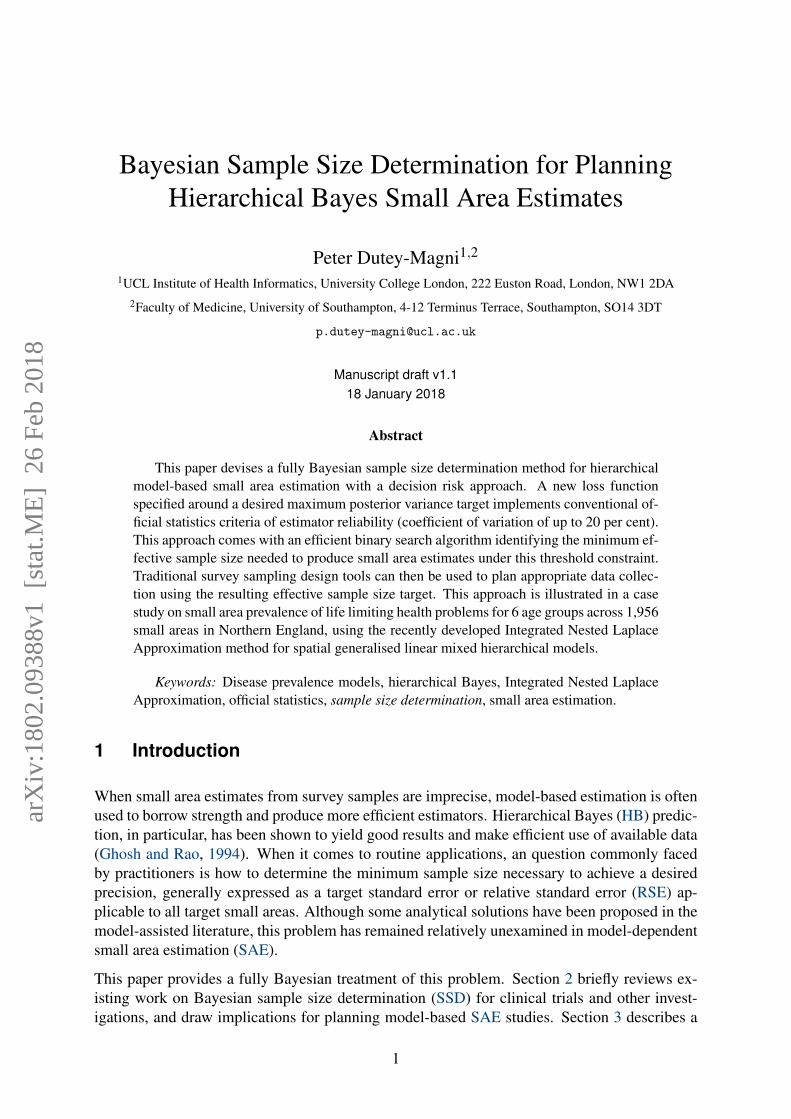
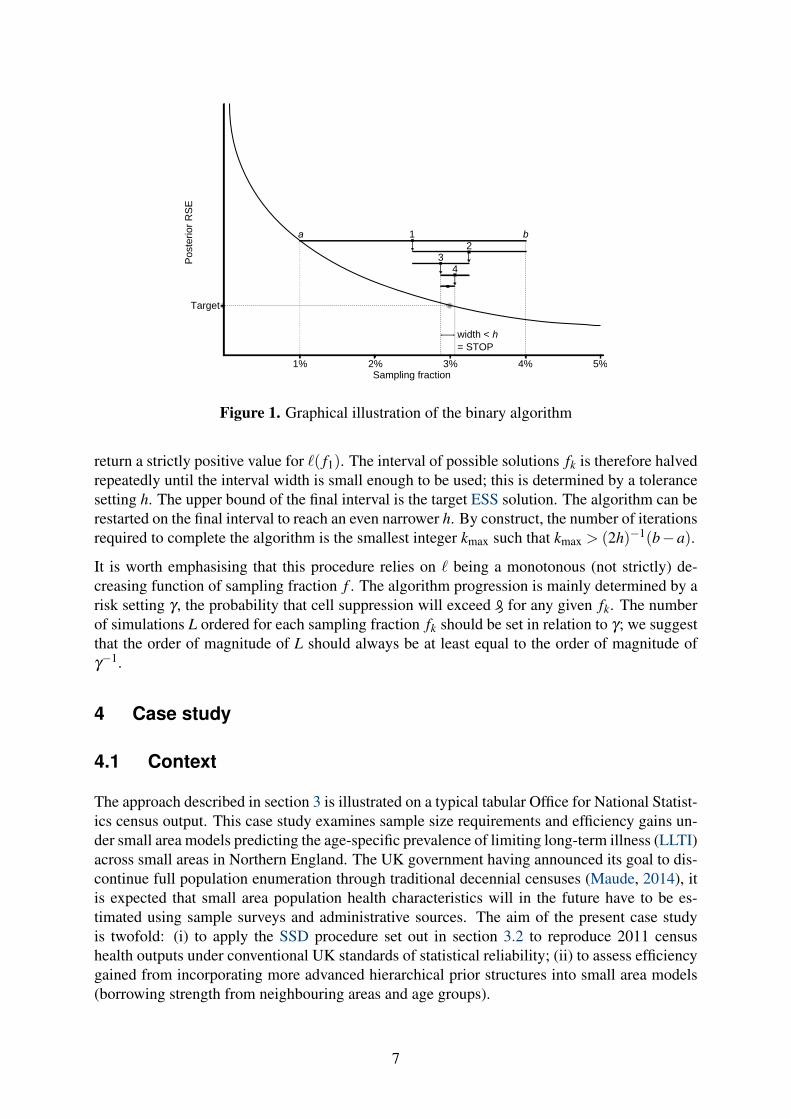
3.2 Sample size minimisation

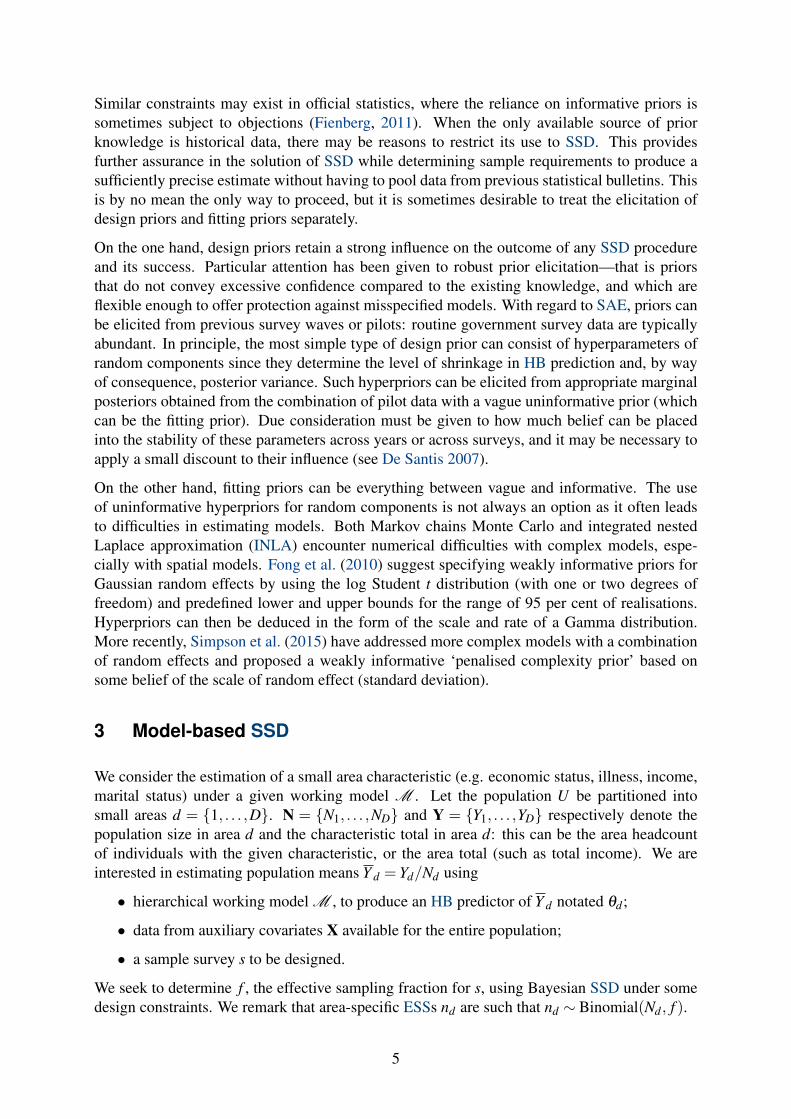
Simulating the relative posterior variance for all possible sample sizes until the minimum qual-ity standard is attained following a sweep approach is computationally cumbersome. We insteadopt for a binary search algorithm (see Figures 1 and 2) to minimise `( f ). By progressing iterat-ively towards the solution with steps of decreasing sizes, we considerably reduce the number ofsimulations. The algorithm starts with f1, the midpoint of the interval [a,b], and evaluates `( f1)over many replications of the sampling and model estimation process. This process is then rep-licated on interval [a, f1] if `( f1) can be trusted to fall below the maximum tolerated suppressionsetting or [ f1,b] in the opposite case—that is, if more than per cent of sampling simulations

6

1% 2% 3% 4% 5%

Target

width < h= STOP

a b

Pos

terio

r RS

E

Sampling fraction

12

34

Figure 1. Graphical illustration of the binary algorithm

return a strictly positive value for `( f1). The interval of possible solutions fk is therefore halvedrepeatedly until the interval width is small enough to be used; this is determined by a tolerancesetting h. The upper bound of the final interval is the target ESS solution. The algorithm can berestarted on the final interval to reach an even narrower h. By construct, the number of iterationsrequired to complete the algorithm is the smallest integer kmax such that kmax > (2h)−1(b−a).

It is worth emphasising that this procedure relies on ` being a monotonous (not strictly) de-creasing function of sampling fraction f . The algorithm progression is mainly determined by arisk setting γ , the probability that cell suppression will exceed for any given fk. The numberof simulations L ordered for each sampling fraction fk should be set in relation to γ; we suggestthat the order of magnitude of L should always be at least equal to the order of magnitude ofγ−1.

4 Case study

4.1 Context

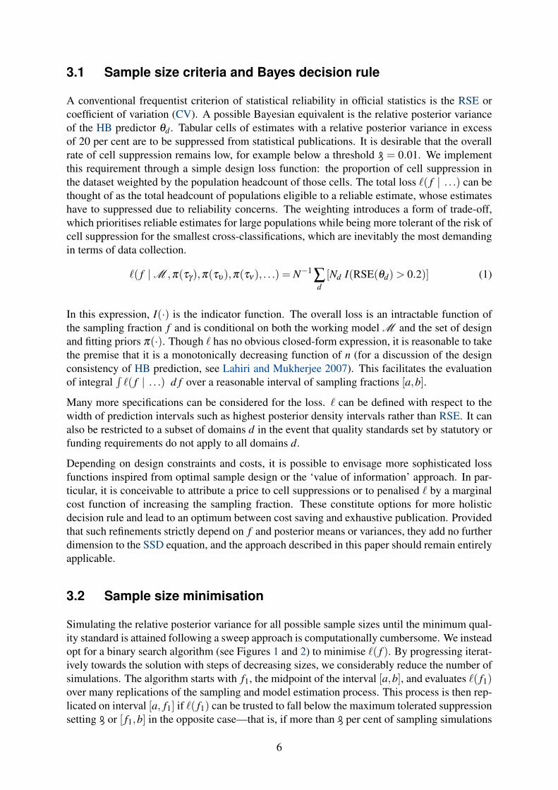
The approach described in section 3 is illustrated on a typical tabular Office for National Statist-ics census output. This case study examines sample size requirements and efficiency gains un-der small area models predicting the age-specific prevalence of limiting long-term illness (LLTI)across small areas in Northern England. The UK government having announced its goal to dis-continue full population enumeration through traditional decennial censuses (Maude, 2014), itis expected that small area population health characteristics will in the future have to be es-timated using sample surveys and administrative sources. The aim of the present case studyis twofold: (i) to apply the SSD procedure set out in section 3.2 to reproduce 2011 censushealth outputs under conventional UK standards of statistical reliability; (ii) to assess efficiencygained from incorporating more advanced hierarchical prior structures into small area models(borrowing strength from neighbouring areas and age groups).

7

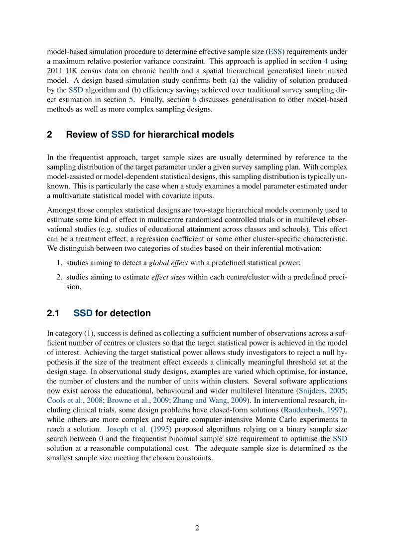
1 Input: s0, π(θd | s0), fa, fb, `( fa), `( fb), h, , L, γ

2 k← 0; l← 0;repeat

3 k← k+1;4 fk← ( fa + fb)/2;

repeat5 l← l +1;6 sample θ ?

d from prior π(θd | s0);7 simulate n?dl ∼ Binomial(Nd, fk);8 simulate n?dl realisations y?dl from the

likelihood of θ ?dl;

9 fit model M ?l on data y?dl ;

10 estimate posterior density π(θ ?dl|y?dl,M

?l ) ;

11 compute relative posterior variancesRSE(θ ?

dl) ;until l = L;

12 `( fk)l ← N−1∑

Dd=1

(Nd I

[RSE(θ ?

dl)> 0.2])

;

if Pr(`( fk)≤ )< γ then13 fb← fk

else14 fa← fk

enduntil fb− fa < h;

15 return fa, fb, `(a), `(b)

Figure 2. Binary SSD algorithm

8

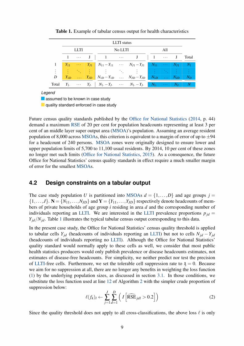
Table 1. Example of tabular census output for health characteristics

LLTI status

LLTI No LLTI All

1 · · · J 1 · · · J 1 · · · J Total

1 Y11 · · · YJ1 N11−Y11 · · · NJ1−YJ1 N11 · · · NJ1 N1...

.... . .

......

. . ....

.... . .

......

D Y1D . . . YJD N1D−Y1D . . . NJD−YJD N1D . . . NJD ND

Total Y1· · · · YJ· N1·−YJ· · · · N1·−YJ· N1· · · · NJ· N

Legendassumed to be known in case studyquality standard enforced in case study

Future census quality standards published by the Office for National Statistics (2014, p. 44)demand a maximum RSE of 20 per cent for population headcounts representing at least 3 percent of an middle layer super output area (MSOA)’s population. Assuming an average residentpopulation of 8,000 across MSOAs, this criterion is equivalent to a margin of error of up to±94for a headcount of 240 persons. MSOA zones were originally designed to ensure lower andupper population limits of 5,700 to 11,100 usual residents. By 2014, 10 per cent of these zonesno longer met such limits (Office for National Statistics, 2015). As a consequence, the futureOffice for National Statistics’ census quality standards in effect require a much smaller marginof error for the smallest MSOAs.

4.2 Design constraints on a tabular output

The case study population U is partitioned into MSOAs d = {1, . . . ,D} and age groups j ={1, . . . ,J}. N = {N11, . . . ,NJD} and Y = {Y11, . . . ,YJD} respectively denote headcounts of mem-bers of private households of age group i residing in area d and the corresponding number ofindividuals reporting an LLTI. We are interested in the LLTI prevalence proportions p jd =Yjd/N jd . Table 1 illustrates the typical tabular census output corresponding to this data.

In the present case study, the Office for National Statistics’ census quality threshold is appliedto tabular cells Yjd (headcounts of individuals reporting an LLTI) but not to cells N jd −Yjd(headcounts of individuals reporting no LLTI). Although the Office for National Statistics’quality standard would normally apply to these cells as well, we consider that most publichealth statistics producers would only publish prevalence or disease headcounts estimates, notestimates of disease-free headcounts. For simplicity, we neither predict nor test the precisionof LLTI-free cells. Furthermore, we set the tolerable cell suppression rate to = 0. Becausewe aim for no suppression at all, there are no longer any benefits in weighting the loss function(1) by the underlying population sizes, as discussed in section 3.1. In those conditions, wesubstitute the loss function used at line 12 of Algorithm 2 with the simpler crude proportion ofsuppression below:

`( fk)l ←J

∑j=1

D

∑d=1

(I[RSE jdl > 0.2

])(2)

Since the quality threshold does not apply to all cross-classifications, the above loss ` is only

9

computed over cross-classifications jd such that Yjd/Nd ≥ 0.03. Because Yjd is in reality un-known, we compute the estimated loss ˆ over cross-classifications jd such that θ jd/Nd ≥ 0.03.We nevertheless report both the true and the estimated loss in results in order to assess anypotential divergence in the algorithm’s progression.

Using data from the 2011 UK census table LC3101EWLS (Office for National Statistics, 2013a),18 age groups were collapsed in order to bring Yjd/Nd to an average level close to 3 per centor more. With D = 1,956 and setting J = 6, we have a total JD = 11,736 cells, 49 per cent ofwhich are eligible for the quality standard of a 20 per cent RSE. Other settings are configuredat fa = 0.01, fb = 0.04, h = 0.01 and L = 100. The acceptable risk of exceeding the tolerablerate of suppression is set to γ = 0.01.

4.3 Model specification

We consider the below working model (3). Sample counts y jd are treated as the realisation of abinomial distribution with sample size n jd and success parameter p jd = logit−1(θ jd).

y jd ∼ Binomial(logit−1(θ jd),n jd

)θ jd = β

(1)j +Xdβ

(2)j +υd +ν jd

(3)

where β (1) is an i-dimensional vector of age contrasts (with β(1)1 = 0 for identifiability); X a

matrix of area-level scaled covariates; β (2) is a matrix of coefficients controlling the effect ofone standard deviation in the covariates on area-level log-odds of LLTI; a structured intrinsicconditional autoregressive (ICAR) area random effect υd; an unstructured (exchangeable) areaby age random effect ν jd .

Covariates in X are taken from public sources; namely: the MSOA- and district-level indirectlystandardised emergency hospital admissions rate (ISAR) (Public Health England, 2014); the2015 Income Deprivation Affecting Children Index (proportion of all children aged 0–15 yearsliving in income-deprived families based on tax and benefit departmental database, PublicHealth England, 2016); the MSOA mean price of residential property sales in 2011 (Officefor National Statistics, 2016a); 2011 mortality ratios indirectly standardised by sex and age(Office for National Statistics, 2013b); and the 2011 MSOA Rural Urban Classification consist-ing of five contrasts (Office for National Statistics, 2016b). No age-specific area covariates wereavailable, which reduces the predictive capabilities of the model: although ISARs exhibit stronglevels of correlation with crude LLTI prevalence across MSOAs, associations with age-specificprevalence are weaker.

The structured ICAR area effect υd is included to model the shared spatial surface in diseaseprevalence as first introduced by Besag (1974) under a sum-to-zero constraint for identifiability:∑

Dd=1 υd = 0. Every structured area effect υd is dependent on other area structured effects

υυυ [d] = {υ j, j 6= d} under the following conditional distribution:

υd | υυυ [d] ∼ Normal

(∑d 6= j

wd jυ j

wd j,

1τυ ∑[d]wd j

)(4)

where spatial weights w are taken from the spatial dependence matrix R−1υ defined as a D×D-

10

0 10 20 30 40

0.00

0.05

0.10

0.15

0.20

0.25

N = 100000 Bandwidth = 0.7321

Den

sity

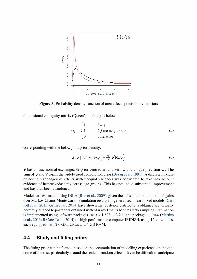
Γ(1, 0.1)Γ(0.5, 0.1)

Figure 3. Probability density function of area effects precision hyperpriors

dimensional contiguity matrix (Queen’s method) as below:

wi j =

1 i = j1 i, j are neighbours0 otherwise

(5)

corresponding with the below joint prior density:

π(υυυ | τυ) ∝ exp(−τυ

2υυυ′Rυυυυ

)(6)

ννν has a basic normal exchangeable prior centred around zero with a unique precision τν . Thesum of υυυ and ννν forms the widely used convolution prior (Besag et al., 1991). A discrete mixtureof normal exchangeable effects with unequal variances was considered to take into accountevidence of heteroskedasticity across age groups. This has not led to substantial improvementand has thus been abandoned.

Models are estimated using INLA (Rue et al., 2009), given the substantial computational gainsover Markov Chains Monte Carlo. Simulation results for generalised linear mixed models (Car-roll et al., 2015; Grilli et al., 2014) have shown that posterior distributions obtained are virtuallyperfectly aligned to posteriors obtained with Markov Chains Monte Carlo sampling. Estimationis implemented using software packages INLA v 1.698, R 3.2.1, and package R-INLA (Martinset al., 2013; R Core Team, 2014) on high performance computer IRIDIS 4, using 16-core nodes,each equipped with 2.6 GHz CPUs and 4 GB RAM.

4.4 Study and fitting priors

The fitting prior can be formed based on the accumulation of modelling experience on the out-come of interest, particularly around the scale of random effects. It can be difficult to anticipate

11

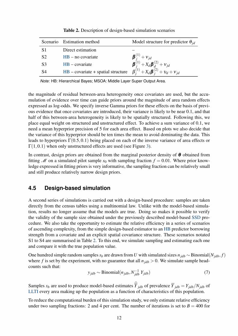
Table 2. Description of design-based simulation scenarios

Scenario Estimation method Model structure for predictor θ jd

S1 Direct estimation –S2 HB – no covariate βββ

(1)j +ν jd

S3 HB – covariate βββ(1)j +Xdβββ

(2)d +ν jd

S4 HB – covariate + spatial structure β(1)j +Xdβββ

(2)j +υd +ν jd

Note: HB: Hierarchical Bayes; MSOA: Middle Layer Super Output Area.

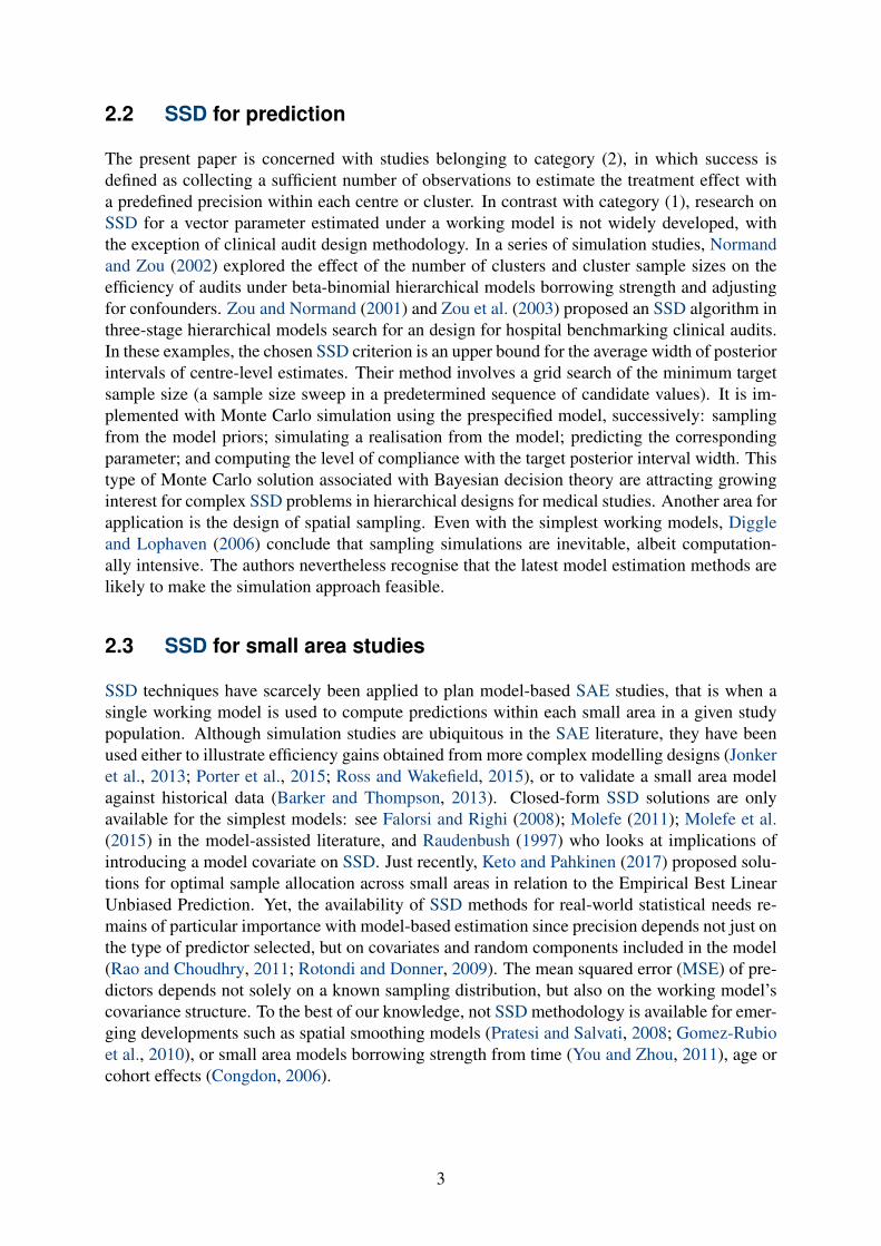
the magnitude of residual between-area heterogeneity once covariates are used, but the accu-mulation of evidence over time can guide priors around the magnitude of area random effectsexpressed as log-odds. We specify inverse Gamma priors for these effects on the basis of previ-ous evidence that once covariates are introduced, their variance is likely to be near 0.1, and thathalf of this between-area heterogeneity is likely to be spatially structured. Following this, weplace equal weight on structured and unstructured effect. To achieve a sum variance of 0.1, weneed a mean hyperprior precision of 5 for each area effect. Based on plots we also decide thatthe variance of this hyperprior should be ten times the mean to avoid dominating the data. Thisleads to hyperpriors Γ(0.5,0.1) being placed on each of the inverse variance of area effects orΓ(1,0.1) when only unstructured effects are used (see Figure 3).

In contrast, design priors are obtained from the marginal posterior density of θθθ obtained fromfitting M on a simulated pilot sample s0 with sampling fraction f = 0.01. Where prior know-ledge expressed in fitting priors is very informative, the sampling fraction can be relatively smalland still produce relatively narrow design priors.

4.5 Design-based simulation

A second series of simulations is carried out with a design-based procedure: samples are takendirectly from the census tables using a multinomial law. Unlike with the model-based simula-tion, results no longer assume that the models are true. Doing so makes it possible to verifythe validity of the sample size obtained under the previously described model-based SSD pro-cedure. We also take the opportunity to estimate the relative efficiency in a series of scenariosof ascending complexity, from the simple design-based estimator to an HB predictor borrowingstrength from a covariate and an explicit spatial covariance structure. These scenarios notatedS1 to S4 are summarised in Table 2. To this end, we simulate sampling and estimating each oneand compare it with the true population value.

One hundred simple random samples sb are drawn from U with simulated sizes n jdb∼Binomial(N jdb, f )where f is set by the experiment, with no guarantee that all n jdb > 0. We simulate sample head-counts such that:

y jdb ∼ Binomial(n jdb,N−1jdb Yjdb) (7)

Samples sb are used to produce model-based estimates Y jdb of prevalence Y jdb = Y jdb/N jdb ofLLTI every area making up the population as a function of characteristics of this population.

To reduce the computational burden of this simulation study, we only estimate relative efficiencyunder two sampling fractions: 2 and 4 per cent. The number of iterations is set to B = 400 for

12

each combination of a scenario and sampling fraction, totalling 2,400 procedures of modelestimation and prediction. For scenarios S2–S5, and for each of the chosen sampling fractionsf , we compute measures of accuracy:

• the root mean squared error (RMSE)

RMSE jd =

√√√√B−1B

∑b=1

(Y jdb−Y jdb

)2(8)

• the bias

Bias jd = B−1B

∑b=1

(Y jdb−Y jdb

)(9)

• the absolute relative bias (absolute relative bias (ARB))

ARB jd = B−1B

∑b=1

|Y jdb−Y jdb|Y jdb

(10)

• the relative RMSE or relative standard error (RSE)

RSE jd =RMSE jd

Y jd(11)

• the RSE’s relative bias (RSEB) (where postMSE is the posterior variance)

RSEB jd = B−1B

∑b=1

RSE jdb−RSE jdb

RSE jdb

RSE jd =

√ postMSE jd

ˆYjd

(12)

These measures are mapped and averaged across small areas d to be reported in tables. Forscenario S1, the bias of sample means is by definition zero and we calculate the MSE and RSEusing the variance formula of the sample proportion:

Var(y jd) =Y (1−Y )

n jd=

Y (1−Y )f N jd

(13)

5 Results

5.1 SSD procedure

The basic model (3) is fitted to pilot sample s0 of ESS n = 146,574, with 1,952 cells jd con-taining no observations. This means no data is available for 1.3 per cent of the total numberof cells, or 8.8 per cent of cells where the minimum quality standard applies. The fitted modelachieves an acceptable deviance information criterion (DIC) of 33,787. The SSD procedure

13

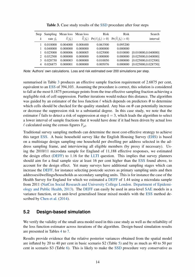
Table 3. Case study results of the SSD procedure after four steps

Step Sampling Mean loss Mean loss Risk Risk Searchk rate fk ¯( fk)

ˆ( fk) Pr(`( fk)> 0) Pr( ˆ( fk)> 0) interval

1 0.010000 0.004000 0.008400 0.063500 0.0952001 0.040000 0.000000 0.000000 0.000000 0.0000001 0.025000 0.000006 0.000005 0.025000 0.010000 [0.010000,0.040000]2 0.032500 0.000000 0.000000 0.000000 0.000000 [0.025000,0.040000]3 0.028750 0.000003 0.000000 0.010050 0.000000 [0.025000,0.032500]4 0.026875 0.000001 0.000000 0.005076 0.000000 [0.025000,0.028750]

Note: Authors’ own calculations. Loss and risk estimated over 200 simulations per step.

summarised in Table 3 produces an effective sample fraction requirement of 2.6875 per cent,equivalent to an ESS of 394,103. Assuming the procedure is correct, this solution is consideredto fall at the most 0.1875 percentage points from the true effective sampling fraction achieving anegligible risk of cell suppression. Further iterations would reduce this distance. The algorithmwas guided by an estimator of the loss function ` which depends on predictors θ to determinewhich cells should be checked for the quality standard. Any bias on θ can potentially increaseor decrease the suppression risk to a substantial degree. In this case study, we note that theestimator ˆ fails to detect a risk of suppression at step k = 3, which leads the algorithm to selecta lower interval of sample fractions that it would have done if it had been driven by actual loss` calculated using the census figures Yjd .

Traditional survey sampling methods can determine the most cost-effective strategy to achievethis target ESS. A basic household survey like the English Housing Survey (EHS) is basedon a multistage design sampling one household per dwelling per address selected in the ad-dress sampling frame, and interviewing all eligible members (by proxy if necessary). Us-ing the 2010/11 microdata sample for England of 11,188 effective responses, we estimatedthe design effect (DEFF) to 1.16 for the LLTI question. This implies that survey plannersshould aim for a final sample size at least 16 per cent higher than the ESS found above, toaccount for the design effect. Yet many surveys have additional sampling stages which canincrease the DEFF, for instance selecting postcode sectors as primary sampling units and thenaddresses/dwellings/households as secondary sampling units. This is for instance the case of theHealth Survey for England for which we estimated a DEFF of 1.44 using a microdata samplefrom 2011 (NatCen Social Research and University College London. Department of Epidemi-ology and Public Health, 2013). The DEFF can easily be used in area-level SAE models in avariance function, or in unit-level generalised linear mixed models with the ESS method de-scribed by Chen et al. (2014).

5.2 Design-based simulation

We verify the validity of the small area model used in this case study as well as the reliability ofthe loss function estimator across iterations of the algorithm. Design-based simulation resultsare presented in Tables 4 to 7.

Results provide evidence that the relative posterior variances obtained from the spatial modelare inflated by 20 to 40 per cent in basic scenario S2 (Table 5) and by as much as 40 to 50 percent in scenario S3 (Table 6). This is likely to make the SSD procedure very conservative as

14

many cells will be unnecessarily suppressed. This is a likely sign of poor model specification.Simulations for other scenarios are reported here to quantify the relative efficiency of the dif-ferent model- and design-based methods. Efficiency savings from using a particularly model orfrom an increase in sample size can be derived as the ratio of RMSE of two scenarios. Compar-ing the scenarios presented in Table 2, we find that even a basic model without area covariates(see S1–S2, Tables 4 and 5) achieves a reduction in root mean squared error (RMSE) by about49 per cent overall, and up to 74 per cent for youngest age groups ( f = 0.02). This comes ata very reasonable computational cost and with a bias of between 0.1 and 0.7 percentage point.With a much larger sample ( f = 0.04), the efficiency gain comes down to approximately 35 percent.

The addition of covariates delivers strong efficiency gains (see S3, Tables 6) with an reductionin RMSE by 72 ( f = 0.02) and 62 per cent ( f = .04). This includes a reduction in bias from0.02 to below 0.01 percentage point.

Comparing results for f = 0.02 and f = 0.04, we note that doubling the sample size has di-minishing returns as the methods becomes more complicated. Whilst it reduces the standarddeviation of design-based estimates S1 by 29 per cent, the RMSE of estimates S2 is only re-duced by 12 per cent. As for estimates S3 and S4 the reduction by less than 3 and 4 per centrespectively is not material for an augmentation of this magnitude. This shows that RMSE asa function of sample size is already relatively horizontal in the regions of sample sizes we areinvestigating, which is not the case for design-based estimators. Regardless of the sample size,bias remains high. Although the average bias across areas remains of the order of 0.1 to 0.3percentage points, the more meaningful ARB metric reveals an average absolute bias of 5 to 20per cent of the target parameter. This represents almost all the total RSE. This bias is not verysensitive to the sampling fraction or the type of between-area variance structure used.

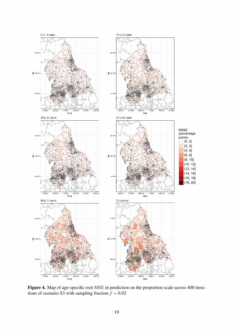
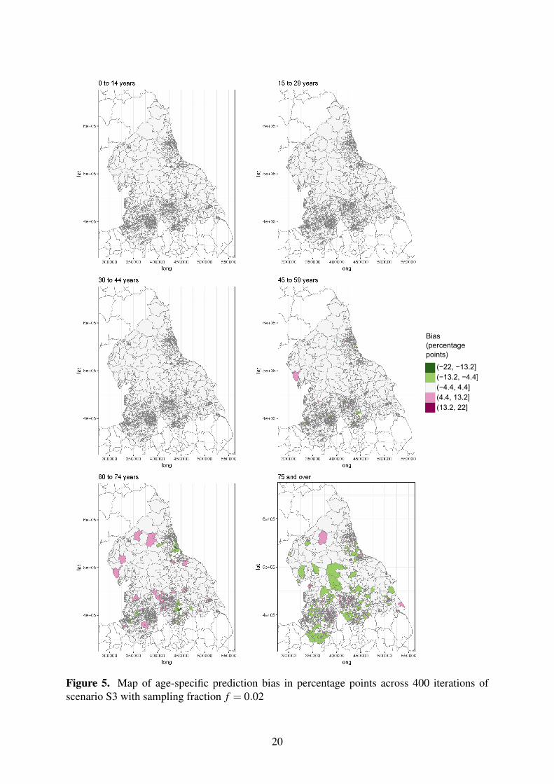
The working model was designed to borrow strength by assuming that areas situated near eachother were more similar. We thus examined simulation results to verify whether this assumptionholds everywhere equally. Figures 4 and 5 present the RMSE and bias for age-specific MSOAprevalence proportion computed from S3 with f = 0.020. Hotpots of high RMSE and bias of1 to 2 percentage points are visible which exhibit a spatial pattern. This could signal outlierareas, or areas in which that covariates are poorly measured and making the linear predictorparticularly biased. The convolution prior used here may not fully and authentically reproducethe spatial pattern of the health status under consideration.

15

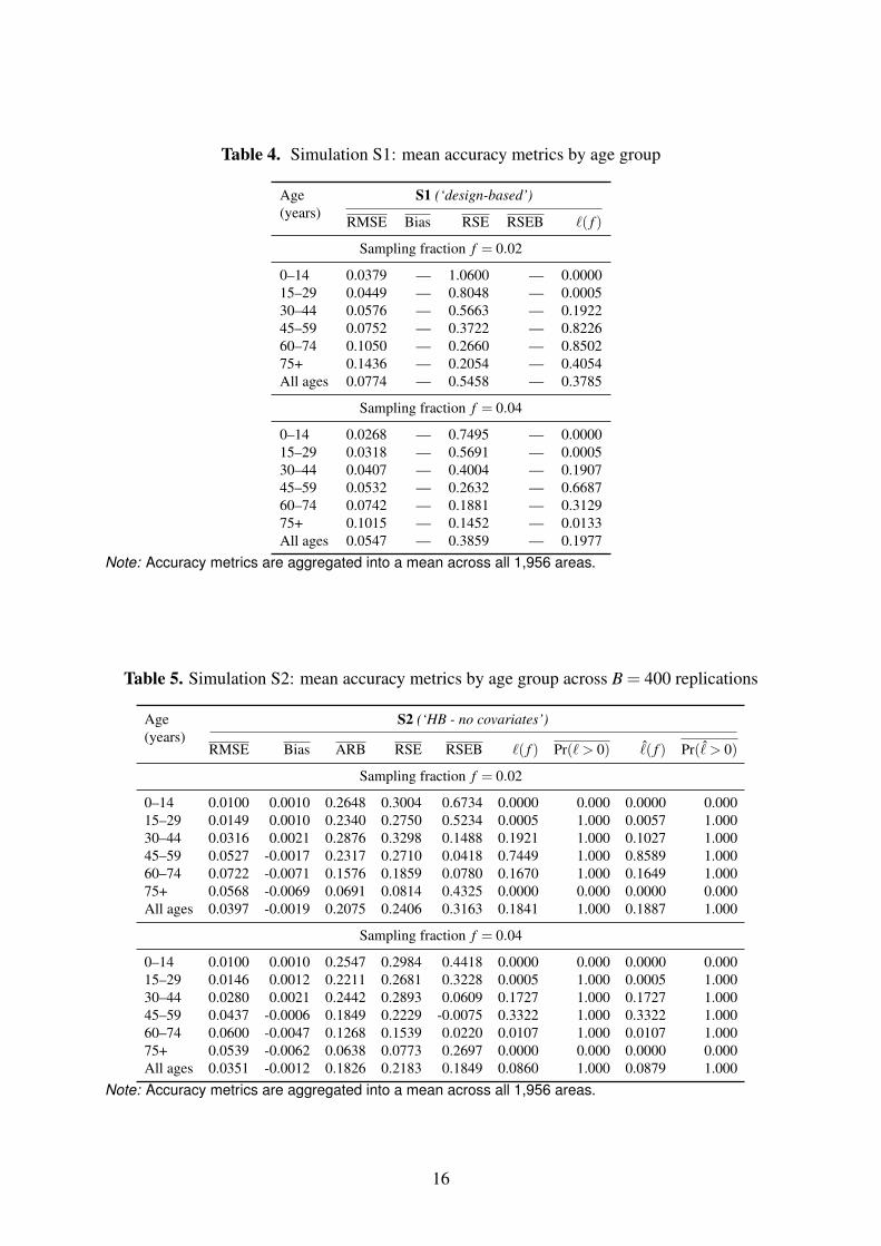
Table 4. Simulation S1: mean accuracy metrics by age group

Age(years)

S1 (‘design-based’)

RMSE Bias RSE RSEB `( f )

Sampling fraction f = 0.02

0–14 0.0379 — 1.0600 — 0.000015–29 0.0449 — 0.8048 — 0.000530–44 0.0576 — 0.5663 — 0.192245–59 0.0752 — 0.3722 — 0.822660–74 0.1050 — 0.2660 — 0.850275+ 0.1436 — 0.2054 — 0.4054All ages 0.0774 — 0.5458 — 0.3785

Sampling fraction f = 0.04

0–14 0.0268 — 0.7495 — 0.000015–29 0.0318 — 0.5691 — 0.000530–44 0.0407 — 0.4004 — 0.190745–59 0.0532 — 0.2632 — 0.668760–74 0.0742 — 0.1881 — 0.312975+ 0.1015 — 0.1452 — 0.0133All ages 0.0547 — 0.3859 — 0.1977

Note: Accuracy metrics are aggregated into a mean across all 1,956 areas.

Table 5. Simulation S2: mean accuracy metrics by age group across B = 400 replications

Age(years)

S2 (‘HB - no covariates’)

RMSE Bias ARB RSE RSEB `( f ) Pr(` > 0) ˆ( f ) Pr( ˆ> 0)

Sampling fraction f = 0.02

0–14 0.0100 0.0010 0.2648 0.3004 0.6734 0.0000 0.000 0.0000 0.00015–29 0.0149 0.0010 0.2340 0.2750 0.5234 0.0005 1.000 0.0057 1.00030–44 0.0316 0.0021 0.2876 0.3298 0.1488 0.1921 1.000 0.1027 1.00045–59 0.0527 -0.0017 0.2317 0.2710 0.0418 0.7449 1.000 0.8589 1.00060–74 0.0722 -0.0071 0.1576 0.1859 0.0780 0.1670 1.000 0.1649 1.00075+ 0.0568 -0.0069 0.0691 0.0814 0.4325 0.0000 0.000 0.0000 0.000All ages 0.0397 -0.0019 0.2075 0.2406 0.3163 0.1841 1.000 0.1887 1.000

Sampling fraction f = 0.04

0–14 0.0100 0.0010 0.2547 0.2984 0.4418 0.0000 0.000 0.0000 0.00015–29 0.0146 0.0012 0.2211 0.2681 0.3228 0.0005 1.000 0.0005 1.00030–44 0.0280 0.0021 0.2442 0.2893 0.0609 0.1727 1.000 0.1727 1.00045–59 0.0437 -0.0006 0.1849 0.2229 -0.0075 0.3322 1.000 0.3322 1.00060–74 0.0600 -0.0047 0.1268 0.1539 0.0220 0.0107 1.000 0.0107 1.00075+ 0.0539 -0.0062 0.0638 0.0773 0.2697 0.0000 0.000 0.0000 0.000All ages 0.0351 -0.0012 0.1826 0.2183 0.1849 0.0860 1.000 0.0879 1.000

Note: Accuracy metrics are aggregated into a mean across all 1,956 areas.

16

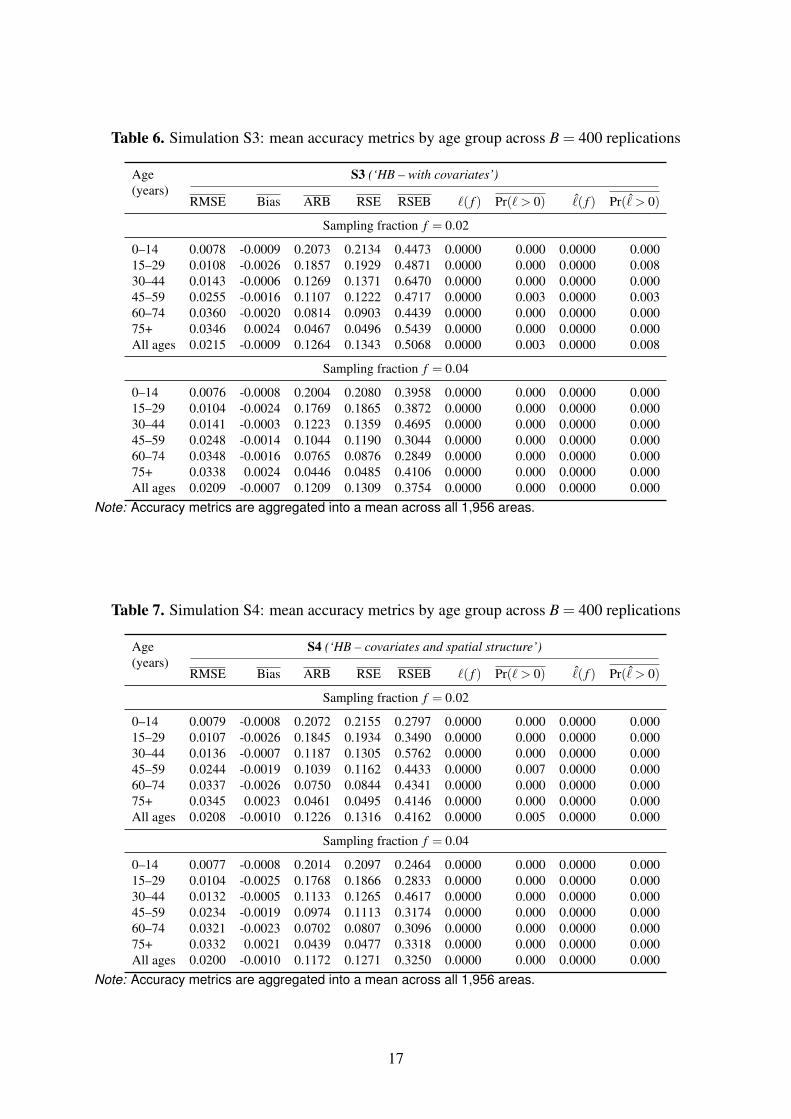
Table 6. Simulation S3: mean accuracy metrics by age group across B = 400 replications

Age(years)

S3 (‘HB – with covariates’)

RMSE Bias ARB RSE RSEB `( f ) Pr(` > 0) ˆ( f ) Pr( ˆ> 0)

Sampling fraction f = 0.02

0–14 0.0078 -0.0009 0.2073 0.2134 0.4473 0.0000 0.000 0.0000 0.00015–29 0.0108 -0.0026 0.1857 0.1929 0.4871 0.0000 0.000 0.0000 0.00830–44 0.0143 -0.0006 0.1269 0.1371 0.6470 0.0000 0.000 0.0000 0.00045–59 0.0255 -0.0016 0.1107 0.1222 0.4717 0.0000 0.003 0.0000 0.00360–74 0.0360 -0.0020 0.0814 0.0903 0.4439 0.0000 0.000 0.0000 0.00075+ 0.0346 0.0024 0.0467 0.0496 0.5439 0.0000 0.000 0.0000 0.000All ages 0.0215 -0.0009 0.1264 0.1343 0.5068 0.0000 0.003 0.0000 0.008

Sampling fraction f = 0.04

0–14 0.0076 -0.0008 0.2004 0.2080 0.3958 0.0000 0.000 0.0000 0.00015–29 0.0104 -0.0024 0.1769 0.1865 0.3872 0.0000 0.000 0.0000 0.00030–44 0.0141 -0.0003 0.1223 0.1359 0.4695 0.0000 0.000 0.0000 0.00045–59 0.0248 -0.0014 0.1044 0.1190 0.3044 0.0000 0.000 0.0000 0.00060–74 0.0348 -0.0016 0.0765 0.0876 0.2849 0.0000 0.000 0.0000 0.00075+ 0.0338 0.0024 0.0446 0.0485 0.4106 0.0000 0.000 0.0000 0.000All ages 0.0209 -0.0007 0.1209 0.1309 0.3754 0.0000 0.000 0.0000 0.000

Note: Accuracy metrics are aggregated into a mean across all 1,956 areas.

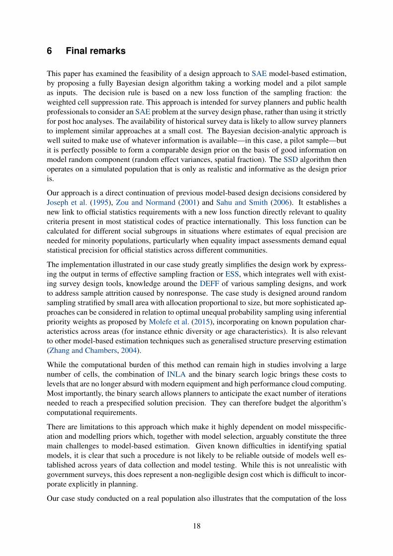
Table 7. Simulation S4: mean accuracy metrics by age group across B = 400 replications

Age(years)

S4 (‘HB – covariates and spatial structure’)

RMSE Bias ARB RSE RSEB `( f ) Pr(` > 0) ˆ( f ) Pr( ˆ> 0)

Sampling fraction f = 0.02

0–14 0.0079 -0.0008 0.2072 0.2155 0.2797 0.0000 0.000 0.0000 0.00015–29 0.0107 -0.0026 0.1845 0.1934 0.3490 0.0000 0.000 0.0000 0.00030–44 0.0136 -0.0007 0.1187 0.1305 0.5762 0.0000 0.000 0.0000 0.00045–59 0.0244 -0.0019 0.1039 0.1162 0.4433 0.0000 0.007 0.0000 0.00060–74 0.0337 -0.0026 0.0750 0.0844 0.4341 0.0000 0.000 0.0000 0.00075+ 0.0345 0.0023 0.0461 0.0495 0.4146 0.0000 0.000 0.0000 0.000All ages 0.0208 -0.0010 0.1226 0.1316 0.4162 0.0000 0.005 0.0000 0.000

Sampling fraction f = 0.04

0–14 0.0077 -0.0008 0.2014 0.2097 0.2464 0.0000 0.000 0.0000 0.00015–29 0.0104 -0.0025 0.1768 0.1866 0.2833 0.0000 0.000 0.0000 0.00030–44 0.0132 -0.0005 0.1133 0.1265 0.4617 0.0000 0.000 0.0000 0.00045–59 0.0234 -0.0019 0.0974 0.1113 0.3174 0.0000 0.000 0.0000 0.00060–74 0.0321 -0.0023 0.0702 0.0807 0.3096 0.0000 0.000 0.0000 0.00075+ 0.0332 0.0021 0.0439 0.0477 0.3318 0.0000 0.000 0.0000 0.000All ages 0.0200 -0.0010 0.1172 0.1271 0.3250 0.0000 0.000 0.0000 0.000

Note: Accuracy metrics are aggregated into a mean across all 1,956 areas.

17

6 Final remarks

This paper has examined the feasibility of a design approach to SAE model-based estimation,by proposing a fully Bayesian design algorithm taking a working model and a pilot sampleas inputs. The decision rule is based on a new loss function of the sampling fraction: theweighted cell suppression rate. This approach is intended for survey planners and public healthprofessionals to consider an SAE problem at the survey design phase, rather than using it strictlyfor post hoc analyses. The availability of historical survey data is likely to allow survey plannersto implement similar approaches at a small cost. The Bayesian decision-analytic approach iswell suited to make use of whatever information is available—in this case, a pilot sample—butit is perfectly possible to form a comparable design prior on the basis of good information onmodel random component (random effect variances, spatial fraction). The SSD algorithm thenoperates on a simulated population that is only as realistic and informative as the design prioris.

Our approach is a direct continuation of previous model-based design decisions considered byJoseph et al. (1995), Zou and Normand (2001) and Sahu and Smith (2006). It establishes anew link to official statistics requirements with a new loss function directly relevant to qualitycriteria present in most statistical codes of practice internationally. This loss function can becalculated for different social subgroups in situations where estimates of equal precision areneeded for minority populations, particularly when equality impact assessments demand equalstatistical precision for official statistics across different communities.

The implementation illustrated in our case study greatly simplifies the design work by express-ing the output in terms of effective sampling fraction or ESS, which integrates well with exist-ing survey design tools, knowledge around the DEFF of various sampling designs, and workto address sample attrition caused by nonresponse. The case study is designed around randomsampling stratified by small area with allocation proportional to size, but more sophisticated ap-proaches can be considered in relation to optimal unequal probability sampling using inferentialpriority weights as proposed by Molefe et al. (2015), incorporating on known population char-acteristics across areas (for instance ethnic diversity or age characteristics). It is also relevantto other model-based estimation techniques such as generalised structure preserving estimation(Zhang and Chambers, 2004).

While the computational burden of this method can remain high in studies involving a largenumber of cells, the combination of INLA and the binary search logic brings these costs tolevels that are no longer absurd with modern equipment and high performance cloud computing.Most importantly, the binary search allows planners to anticipate the exact number of iterationsneeded to reach a prespecified solution precision. They can therefore budget the algorithm’scomputational requirements.

There are limitations to this approach which make it highly dependent on model misspecific-ation and modelling priors which, together with model selection, arguably constitute the threemain challenges to model-based estimation. Given known difficulties in identifying spatialmodels, it is clear that such a procedure is not likely to be reliable outside of models well es-tablished across years of data collection and model testing. While this is not unrealistic withgovernment surveys, this does represent a non-negligible design cost which is difficult to incor-porate explicitly in planning.

Our case study conducted on a real population also illustrates that the computation of the loss

18

RMSE(percentage points)

(0, 2]

(2, 4](4, 6](6, 8](8, 10](10, 12](12, 14](14, 16](16, 18](18, 20]

Figure 4. Map of age-specific root MSE in prediction on the proportion scale across 400 itera-tions of scenario S3 with sampling fraction f = 0.02

19

Bias(percentagepoints)

(−22, −13.2]

(13.2, 22](4.4, 13.2](−4.4, 4.4](−13.2, −4.4]

Figure 5. Map of age-specific prediction bias in percentage points across 400 iterations ofscenario S3 with sampling fraction f = 0.02

20

function being dependent on the reliability of the model, model diagnostics and validation areessential to the reliability and stability of the procedure. Results from the design-based simu-lation studies show the influence of typical model misspecification on estimation bias and howit clusters in space or social groups. Prior formation also remains, as in many other areas ofstatistics, a challenge. Recent work in this area by Fong et al. (2010) and Simpson et al. (2015)expresses some of the important obstacles faced by practitioners in this area.

This work tends to support other research showing the feasibility of reconciling Bayesian infer-ence and survey sampling, the intersection of which, in this case, is expressed in terms of ESS.This also opens perspectives to combine survey sampling with some very strong developmentswitnessed in recent years in the design of experiments literature, particularly around adaptivetrial designs.

Acknowledgements

The author would like to thank Professor Sujit Sahu and Doctor Marta Blangiardo for theirhelpful comments on an early draft. The author acknowledges the use of the IRIDIS High Per-formance Computing Facility, and associated support services at the University of Southampton,in the completion of this work.

Funding

This work was supported by an Economic & Social Research Council, Advanced QuantitativeMethods doctoral studentship [reference number 1223155].

Abbreviations

ARB absolute relative bias

CV coefficient of variation

DEFF design effect

DIC deviance information criterion

EHS English Housing Survey

ESS effective sample size

HB hierarchical Bayes

ICAR intrinsic conditional autoregressive

INLA integrated nested Laplace approximation

ISAR indirectly standardised emergency hospital admissions rate

LLTI limiting long-term illness

MSE mean squared error

MSOA middle layer super output area

RMSE root mean squared error

21

RSE relative standard error

SAE small area estimation

SSD sample size determination

References

Adcock, C. J. (1988). A Bayesian approach to calculating sample sizes. Journal of the Royal Statistical Society:Series D (The Statistician), 37(4/5), 433–439.

Adcock, C. T. (1997). Sample size determination: A review. The Statistician, 46(2), 261–283. DOI: 10.1111/1467-9884.00082.

Barker, L. & Thompson, T. (2013). Bayesian small area estimates of diabetes incidence by United States county,2009. Journal of Data Science, 11(1), 249–267.

Besag, J. (1974). Spatial interaction and the statistical analysis of lattice systems. Journal of the Royal StatisticalSociety. Series B (Statistical Methodology), 36(2), 192–236.

Besag, J., York, J., & Mollie, A. (1991). Bayesian image restoration, with two applications in spatial statistics.Annals of the Institute of Statistical Mathematics, 43(1), 1–20. DOI: 10.1007/BF00116466.

Browne, W. J., Lahi, M. G., & Parker, R. M. (2009). A Guide to Sample Size Calculations for Random EffectModels Via Simulation and the MLPowSim Software Package. University of Bristol, Bristol. URL: http://www.bristol.ac.uk/media-library/sites/cmm/migrated/documents/mlpowsim-manual.pdf [Ac-cessed: 2-2-2017].

Carroll, R., Lawson, A. B., Faes, C., Kirby, R. S., Aregay, M., & Watjou, K. (2015). Comparing INLA andOpenBUGS for hierarchical Poisson modeling in disease mapping. Spatial and Spatio-Temporal Epidemiology,14-15, 45–54. DOI: 10.1016/j.sste.2015.08.001.

Chen, C. X., Wakefield, J., Lumely, T., Lumley, T., & Wakefield, J. (2014). The use of sampling weights inBayesian hierarchical models for small area estimation. DOI: 10.1016/j.sste.2014.07.002.

Congdon, P. (2006). A model framework for mortality and health data classified by age, area, and time. Biometrics,62(1), 269–278. DOI: 10.1111/j.1541-0420.2005.00419.x.

Cools, W., Van den Noortgate, W., & Onghena, P. (2008). ML-DEs: A program for designing efficient multilevelstudies. Behavior Research Methods, 40(1), 236–249. DOI: 10.3758/BRM.40.1.236.

De Santis, F. (2007). Using historical data for Bayesian sample size determination. Journal of the Royal StatisticalSociety: Series A (Statistics in Society), 170(1), 95–113. DOI: 10.1111/j.1467-985X.2006.00438.x.

Diggle, P. & Lophaven, S. (2006). Bayesian geostatistical design. Scandinavian Journal of Statistics, 33(1), 53–64.DOI: 10.1111/j.1467-9469.2005.00469.x.

Falorsi, P. D. & Righi, P. (2008). A balanced sampling approach for multi-way stratification designs for small areaestimation. Survey Methodology, 34(2), 223–234.

Fienberg, S. E. (2011). Bayesian models and methods in public policy and government settings. Statistical Science,26(2), 212–226. DOI: 10.1214/10-STS331.

Fong, Y., Rue, H., & Wakefield, J. (2010). Bayesian inference for generalized linear mixed models. Biostatistics,11(3), 397–412. DOI: 10.1093/biostatistics/kxp053.

Ghosh, M. & Rao, J. N. K. (1994). Small area estimation: An appraisal. Statistical Science, 9(1), 55–76.Gomez-Rubio, V., Best, N., Richardson, S., Li, G., & Clarke, P. (2010). Bayesian statistics for small area estima-

tion. URL: http://eprints.ncrm.ac.uk/1686/ [Accessed: 2-2-2017].Grilli, L., Metelli, S., & Rampichini, C. (2014). Bayesian estimation with Integrated Nested Laplace Approxim-

ation for binary logit mixed models. Journal of Statistical Computation and Simulation, (August 2015), 1–9.DOI: 10.1080/00949655.2014.935377.

Hastings, D. (2002). Annual local area labour force survey data for 2000/2001. Labour Market Trends, 110(1),33–41. URL: http://www.ons.gov.uk/ons/rel/lms/labour-market-trends--discontinued-/

volume-110--no--1/labour-market-trends.pdf [Accessed: 2-2-2017].Jonker, M. F., Congdon, P. D., van Lenthe, F. J., Donkers, B., Burdorf, A., & Mackenbach, J. P. (2013). Small-area

health comparisons using health-adjusted life expectancies: A Bayesian random-effects approach. Health &Place, 23, 70–78. DOI: 10.1016/j.healthplace.2013.04.003.

Joseph, L., Wolfson, D. B., & Du Berger, R. (1995). Sample size calculations for binomial proportions via highestposterior density intervals. Journal of the Royal Statistical Society: Series D (The Statistician), 44(2), 143–154.

22

Keto, M. & Pahkinen, E. (2017). On overall sampling plan for small area estimation. Statistical Journal of theIAOS, 33(3), 727–740. DOI: 10.3233/SJI-170370.

Lahiri, P. & Mukherjee, K. (2007). On the design-consistency property of hierarchical Bayes estimators in finitepopulation sampling. The Annals of Statistics, 35(2), 724–737. DOI: 10.1214/009053606000001262.

Martins, T. G., Simpson, D., Lindgren, F., & Rue, H. (2013). Bayesian computing with INLA: New features.Computational Statistics & Data Analysis, 67, 68–83. DOI: 10.1016/j.csda.2013.04.014.

Maude, F. (2014). Government’s response to the national statistician’s re-commendation. letter to sir andrew dilnot. 18 july 2014. URL: https://www.

statisticsauthority.gov.uk/archive/reports---correspondence/correspondence/

letter-from-rt-hon-francis-maude-mp-to-sir-andrew-dilnot---180714.pdf [Accessed:2-2-2017].

Molefe, W. B. (2011). Sample Design for Small Area Estimation. A thesis submitted in fulfilment of the re-quirements for the award of the degree of doctor of philosophy, University Of Wollongong. URL: http://ro.uow.edu.au/theses/3495 [Accessed: 2-2-2017].

Molefe, W. B., Shangodoyin, D. K., & Clark, R. G. (2015). An approximation to the optimal subsample allocationfor small areas. Statistics in Transition new series, 16(2), 163182.

NatCen Social Research & University College London. Department of Epidemiology and Public Health (2013).Health Survey for England, 2011 [data collection]. SN: 7260. 1st edition, April 2013. Colchester, Essex: UKData Archive [distributor]. DOI: 10.5255/UKDA-SN-7260-1.

Normand, S.-L. T. & Zou, K. H. (2002). Sample size considerations in observational health care quality studies.Statistics in Medicine, 21(3), 331–345. DOI: 10.1002/sim.1020.

Office for National Statistics (2013a). 2011 Census Local Characteristics Table LC3101EWLS (Long Term HealthProblem or Disability by Sex by Age). URL: https://www.nomisweb.co.uk/census/2011/lc3101ewls[Accessed: 2-2-2017].

Office for National Statistics (2013b). Mortality statistics: Deaths registered in England andWales by area of usual residence, 2011. URL: http://www.ons.gov.uk/ons/rel/vsob1/

deaths-registered-area-usual-residence/2011/index.html [Accessed: 2-2-2017].Office for National Statistics (2014). Beyond 2011: Final options report O4. april 2014.

URL: http://www.ons.gov.uk/ons/about-ons/who-ons-are/programmes-and-projects/

beyond-2011/reports-and-publications/methods-and-policies-reports/

beyond-2011--final-options-report.pdf [Accessed: 2-2-2017].Office for National Statistics (2015). Mid-2014 population estimates for Middle Layer Su-

per Output Areas in England and Wales by single year of age and sex. URL: https://

www.ons.gov.uk/file?uri=/peoplepopulationandcommunity/populationandmigration/

populationestimates/datasets/middlesuperoutputareamidyearpopulationestimates/

mid2014/rft-msoa-unformatted-table-2014.zip [Accessed: 2-2-2017].Office for National Statistics (2016a). Mean House Price by Middle Layer Super Output Areas – House Price

Statistics for Small Areas Dataset 3). URL: https://www.ons.gov.uk/peoplepopulationandcommunity/housing/datasets/hpssadataset3meanhousepricebymsoaquarterlyrollingyear [Accessed: 2-2-2017].

Office for National Statistics (2016b). Rural Urban Classification (2011) of Middle Layer Super Output Areas inEngland and Wales. Last Modified: November 9, 2016. URL: http://ons.maps.arcgis.com/home/item.html?id=86fac76c60ed4943a8b94f64bff3e8b1 [Accessed: 2-2-2017].

Porter, A. T., Wikle, C. K., & Holan, S. H. (2015). Small area estimation via multivariate Fay-Herriot models withlatent spatial dependence. Australian & New Zealand Journal of Statistics, 57(1), 15–29. DOI: 10.1111/anzs.12101.

Pratesi, M. & Salvati, N. (2008). Small area estimation: The EBLUP estimator based on spatially correlated ran-dom area effects. Statistical Methods & Applications, 17(1), 113–141. DOI: 10.1007/s10260-007-0061-9.

Public Health England (2014). Emergency Hospital Admissions (All Causes), Indirectly Age Standardised Ra-tio, All Ages, Persons. April 2008 to March 2013 (Inclusive). URL: http://www.localhealth.org.uk/Spreadsheets/Emergencyhospitaladmissionsforallcauses_July2014.xls [Accessed: 2-2-2017].

Public Health England (2016). Child Poverty – Index of Multiple Deprivation (IMD) 2015 Income Deprivation Af-fecting Children Index (IDACI). URL: http://localhealth.org.uk/Spreadsheets/Deprivation%20-%20IMD%202015%20income%20domain_March2016.xlsx [Accessed: 2-2-2017].

R Core Team (2014). R: A Language and Environment for Statistical Computing. R Foundation for StatisticalComputing, Vienna, Austria. URL: http://www.r-project.org/ [Accessed: 2-2-2017].

23

Rao, J. N. K. & Choudhry, G. H. (2011). Small-area estimation: Overview and empirical study. In Cox, B. G.,Binder, D. A., Chinnappa, B. N., Christianson, A., Colledge, M. J., & Kott, P. S., editors, Business SurveyMethods, pages 527–542. John Wiley & Sons, Inc., Hoboken, NJ, USA. DOI: 10.1002/9781118150504.ch27.

Raudenbush, S. W. (1997). Statistical analysis and optimal design for cluster randomized trials. PsychologicalMethods, 2(2), 173–185. DOI: 10.1037/1082-989X.2.2.173.

Ross, M. & Wakefield, J. (2015). Bayesian hierarchical models for smoothing in two-phase studies, with applic-ation to small area estimation. Journal of the Royal Statistical Society: Series A (Statistics in Society), 178(4),1009–1023. DOI: 10.1111/rssa.12103.

Rotondi, M. S. & Donner, A. (2009). Sample size estimation in cluster randomized educational trials: An em-pirical Bayes approach. Journal of Educational and Behavioral Statistics, 34(2), 229–237. DOI: 10.3102/1076998609332756.

Rue, H., Martino, S., & Chopin, N. (2009). Approximate Bayesian inference for latent gaussian models by us-ing Integrated Nested Laplace Approximations. Journal of the Royal Statistical Society: Series B (StatisticalMethodology), 71(2), 319–392. DOI: 10.1111/j.1467-9868.2008.00700.x.

Sahu, S. K. & Smith, T. M. F. (2006). A Bayesian method of sample size determination with practical applications.Journal of the Royal Statistical Society: Series A (Statistics in Society), 169(2), 235–253. DOI: 10.1111/j.1467-985X.2006.00408.x.

Simpson, D. P., Rue, H., Martins, T. G., Riebler, A., & Sørbye, S. H. (2015). Penalising model componentcomplexity: A principled, practical approach to constructing priors. (v4, 6 aug 2015). URL: http://arxiv.org/abs/1403.4630 [Accessed: 2-2-2017].

Snijders, T. A. B. (2005). Power and sample size in multilevel modeling. Encyclopedia of Statistics in BehavioralScience. Volume 3., 3, 1570–1573.

Spiegelhalter, D. J. & Freedman, L. S. (1986). A predictive approach to selecting the size of a clinical trial, basedon subjective clinical opinion. Statistics in Medicine, 5(1), 1–13. DOI: 10.1002/sim.4780050103.

You, Y. & Zhou, Q. M. (2011). Hierarchical Bayes small area estimation under a spatial model with application tohealth survey data. Survey Methodology, 37(1), 25–37.

Zhang, L.-C. & Chambers, R. L. (2004). Small area estimates for cross-classifications. Journal of the RoyalStatistical Society. Series B (Methodological), 66(2), 479–496. DOI: 10.1111/j.1369-7412.2004.05266.x.

Zhang, Z. & Wang, L. (2009). Statistical power analysis for growth curve models using sas. Behavior ResearchMethods, 41(4), 1083–1094. DOI: 10.3758/BRM.41.4.1083.

Zou, K. H. & Normand, S. L. T. (2001). On determination of sample size in hierarchical binomial models. Statisticsin Medicine, 20(14), 2163–2182. DOI: 10.1002/sim.855.

Zou, K. H., Resnic, F. S., Gogate, A. S., & Ondategui-Parra, S. (2003). Efficient Bayesian sample size calculationfor designing a clinical trial with multi-cluster outcome data. Biometrical Journal, 45(7), 826–836. DOI: 10.1002/bimj.200390052.

24