introduction to numerical algebraic geometryjan/articles/intro.pdfintroduction to numerical...

Introduction to Numerical Algebraic Geometry

Andrew J. Sommese1?, Jan Verschelde2??, and Charles W. Wampler3

1 Department of Mathematics, University of Notre Dame, Notre Dame, IN46556-4618, USA. [email protected] http://www.nd.edu/~sommese

2 Department of Mathematics, Statistics, and Computer Science, University ofIllinois at Chicago, 851 South Morgan (M/C 249), Chicago, IL 60607-7045, [email protected] [email protected]

http://www.math.uic.edu/~jan3 General Motors Research and Development, Mail Code 480-106-359, 30500Mound Road, Warren, MI 48090-9055, USA. [email protected]

Abstract. In a 1996 paper, Andrew Sommese and Charles Wampler begandeveloping a new area, “Numerical Algebraic Geometry”, which would bearthe same relation to “Algebraic Geometry” that “Numerical Linear Algebra”bears to “Linear Algebra”.

To approximate all isolated solutions of polynomial systems, numericalpath following techniques have been proven reliable and efficient during thepast two decades. In the nineties, homotopy methods were developed to exploitspecial structures of the polynomial system, in particular its sparsity. Forsparse systems, the roots are counted by the mixed volume of the Newtonpolytopes and computed by means of polyhedral homotopies.

In Numerical Algebraic Geometry we apply and integrate homotopy con-tinuation methods to describe solution components of polynomial systems. Inparticular, our algorithms extend beyond just finding isolated solutions to alsofind all positive dimensional solution sets of polynomial systems and to de-compose these into irreducible components. These methods can be consideredas symbolic-numeric, or perhaps rather as numeric-symbolic, since numericalmethods are applied to find integer results, such as the dimension and degreeof solution components, and via interpolation, to produce symbolic results inthe form of equations describing the irreducible components.

Applications from mechanical engineering motivated the development ofNumerical Algebraic Geometry. The performance of our software on severaltest problems illustrates the effectiveness of the new methods.

? This material is based upon work supported by the National Science Foundationunder Grant No. 0105653; and the Duncan Chair of the University of Notre Dame.

?? This material is based upon work supported by the National Science Foundationunder Grant No. 0105739 and Grant No. 0134611.

2 Andrew J. Sommese, Jan Verschelde, and Charles W. Wampler

1 Introduction

The goal of this paper is to provide an overview of the main ideas developedso far in our research program to implement numerical algebraic geometry,initiated in [SW96].

We are concerned with numerically solving polynomial systems. While thehomotopy continuation methods of the past were limited to approximatingonly the isolated roots, we developed tools to describe all positive dimensionalirreducible components of the solution set of a polynomial system. In partic-ular, our algorithms produce for every irreducible component a witness set,whose cardinality equals the degree of the component, as this set is obtainedby intersecting the component with a general linear space of complementarydimension. A point of a witness set corresponds to what is known in algebraicgeometry as a generic point. Our main results [SV00, SVW01a, SVW01b,SVW01c, SVW02c, SVW02b, SVW02a, SVW03c, SVW03a, SVW03b] can besummarized in four items:

1. In [SV00] we presented a cascade of homotopies (extended in [SVW03a]) tofind candidate witness points for every component of the solution set. Sep-arating the junk from the candidate witness points was done in [SVW01a],where factorization methods based on interpolation implemented a numer-ical irreducible decomposition. The use of central projections and a homo-topy membership test to filter junk were the improvements of [SVW01b].

2. The treatment of high-degree components and components of multiplic-ity greater than one can present numerical challenges. The use of mon-odromy [SVW01c] followed by the validation by the linear trace [SVW02c]enabled us to deal with high degree components of multiplicity one, usingonly machine floating point numbers. In [SVW02b], we presented an ap-proach to tracking paths on sets of multiplicity greater than one, which intheory makes the algorithm for irreducible decomposition completely gen-eral, although in practice this portion of the framework needs further re-finement. However, for the case of the factorization of a single multivariatepolynomial, we can use differentiation to reduce the treatment of highermultiplicity components to nonsingular path tracking, as we describedin [SVW03b]. This addresses an open problem in symbolic-numeric com-puting: the factorization of multivariate polynomials with approximatecoefficients [Kal00].

3. Our new homotopy algorithms have been implemented and tested usingthe path trackers in the software package PHCpack [Ver99a]. In [SVW03c]we outlined the new tools in PHCpack and described a simple interfaceto Maple. Our software found the degrees of all irreducible componentsof the cyclic 8 and 9 roots problems, which previously could only be donevia Grobner bases (and only by the very best implementation [Fau99]).

4. Polynomial systems with positive dimensional components occur natu-rally when designing mechanical devices which permit motion. We inves-

November 2, 2003. Introduction to Numerical Algebraic Geometry 3

tigated a special case of a moving platform, discovering through a nu-merical irreducible decomposition [SVW02c] a component not reportedby experts [HK00]. This and other applications of our tools to systemscoming from mechanical design are described in [SVW02a].

In this paper we will introduce these results, first explaining homotopy meth-ods for isolated solutions. We can only mention some recent and excitingnew developments in fields related to numerical algebraic geometry: numericalSchubert calculus ([HSS98], [HV00], [LWW02], [SS01], [VW02]) and numericaljet geometry [RSV02].Acknowledgements. The authors thank Alicia Dickenstein and IoannisEmiris for their invitation to present their work at the summer school. Weare grateful to Dan Bates for his careful reading and comments. The revi-sion benefited greatly from the stimulating questions from Olga Kashcheyeva,Anton Leykin, Yusong Wang, and Ailing Zhao at the MCS 595 graduate semi-nar. Some of the exercises were first presented at the RAAG summer school onComputer Tools for Real Algebraic Geometry, June 30-July 5, 2003, organizedby Michel Coste, Laureano Gonzalez-Vega, Fabrice Rouillier, Marie-FrancoiseRoy, and Markus Schweighofer, whom we thank for their invitation.

2 Homotopy Continuation Methods – an Overview

Homotopy continuation methods operate in two stages. Firstly, homotopymethods exploit the structure of the system f(x) = 0 to find a root countand to construct a start system g(x) = 0 that has exactly as many regularsolutions as the root count. This start system is embedded in the homotopy

h(x, t) = γ(1− t)g(x) + tf(x) = 0, t ∈ [0, 1], (1)

with γ ∈ C a random number. Secondly, as t moves from 0 to 1, numericalcontinuation methods trace the paths that originate at the solutions of thestart system towards the solutions of the target system. The good propertieswe expect from a homotopy are (borrowed from [Li97, Li03]):

1. (triviality) The solutions for t = 0 are trivial to find.2. (smoothness) No singularities along the solution paths occur (because

of γ).3. (accessibility) An isolated solution of multiplicitym is reached by exactly

m paths.Continuation or path-following methods are standard numerical techniques

([AG90, AG93, AG97], [Mor87], [Wat86, Wat89]) to trace the solution pathsdefined by the homotopy using predictor-corrector methods. The smoothnessproperty of complex polynomial homotopies implies that paths never turnback, so that during correction the parameter t stays fixed, which simplifiesthe set up of path trackers. The adaptive step size control determines thestep length while enforcing quadratic convergence in Newton’s method to


avoid path crossing (see also [KX94] for the application of interval methodsto control the step size). At the end of the path, end games ([HV98], [MSW91,MSW92a, MSW92b], [SWS96]) deal with diverging paths and paths leadingto singular roots.

Following [HSS98], we say that a homotopy is optimal if every path leadsto one solution. The classification in Table 1 (from [Ver99b]) contains keywords for three classes of polynomial systems for which optimal homotopiesare available in PHCpack [Ver99a]. These homotopies have no diverging pathsfor generic instances of polynomial systems in their class.

system model theory space

dense highest degrees Bezout� n projective

sparse Newton polytopes Bernshteın ( � ∗ )n toric

determinantal localization posets Schubert Gmr Grassmannian

Table 1. Key words of the three classes of polynomial systems.

The earliest applications of homotopies for solving polynomial systems([CMPY79], [Dre77], [GZ79], [GL80], [Li83], [LS87] [Mor83], [Wri85], [Zul88])belong to the dense class, where the number of paths equals the product ofthe degrees in the system. Multi-homogeneous homotopies were introducedin [MS87b, MS87a] and applied in [WMS90, WMS92], see also [Wam92]. Sim-ilar are the random product homotopies [LSY87a, LSY87b], see also [Li87]and [LW91]. Methods to construct linear-product start systems were intro-duced in [VH93], and extended in [VC93, VC94], [LWW96], and [WSW00]. Ageneral approach to exploit product structures was developed in [MSW95].

Almost all systems have fewer terms than allowed by their degrees. Im-plementing constructive proofs of Bernshteın’s theorems [Ber75], polyhedralhomotopies were introduced in [HS95] and [VVC94] to solve sparse sys-tems more efficiently. These methods provided ways to start cheater’s ho-motopies ([LSY89], [LW92]) and special instances of coefficient-parameterpolynomial continuation ([MS89, MS90]). The root count requires the cal-culation of the mixed volume4, for which a lift-and-prune approach waspresented in [EC95]. Exploitation of symmetry was studied in [VG95] andthe dynamic lifting of [VGC96] led to incremental polyhedral continuation.See [Ver00] for a Toric Newton. Extensions to count all affine roots (also thosewith zero components) were proposed in [EV99], [GLW99], [HS97], [LW96],[Roj94, Roj99], and [RW96]. Very efficient calculations of mixed volumes aredescribed in [DKK03], [GL00, GL03], [KK03], [LL01], and [TKF02].

Determinantal systems (with equations like det(A|X) = 0) arise in prob-lems of enumerative geometry. The homotopies in numerical Schubert calculus

4 The mixed volume was nicknamed in [CR91] as the BKK bound to honor Bern-shteın [Ber75], Kushnirenko [Kus76], and Khovanskiı [Kho78].


first appeared explicitly in [HSS98], originating from questions in real enumer-ative geometry [Sot97a, Sot97b]. While real enumerative geometry [Sot03]is interesting on its own, these homotopies solve the pole placement prob-lem ([Byr89], [RRW96, RRW98], [Ros94], [RW99]) in control theory. Recentimprovements and applications can be found in [HV00], [LWW02], [SS01],and [VW02].

We end this section noting that homotopies have a wider applicationrange than “just” solving polynomial systems, see for instance [Wat02] fora survey, [WBM87], and [WSM+97] for a description of HOMPACK. Thespeedup of continuation methods on multi-processor machines has been ad-dressed in [ACW89, CARW93, HW89].

3 Homotopies to Approximate All Isolated Solutions

We first prove the regularity and boundedness of the solution paths definedby homotopies, before surveying path following techniques. We obtain moreefficient homotopies by exploiting product structures and using Newton poly-topes to model the sparsity of the system.

3.1 Regularity and Boundedness of Solution Paths

To illustrate how homotopy methods work, let us consider a simple exampleof solving two quadrics:

f(x, y) =

(x2 + 4y2 − 4

2y2 − x

). (2)

To solve f(x, y) = 0, we match it with a start system of two easily solvedquadrics:

g(x, y) =

(x2 − 1y2 − 1

), (3)

with which we form the following homotopy:

h(x, y, t) =

(x2 − 1y2 − 1

)(1− t) +

(x2 + 4y2 − 4

2y2 − x

)t. (4)

At t = 1, h(x, y, t = 1) = 0 is f(x, y) = 0, the system we wish to solve whileat t = 0, h(x, y, t = 0) = 0 is the start system g(x, y) = 0 we can easily solve.As we usually move t from 0 to 1 when we solve the system, we may view themovement of t from 1 to 0 as a degeneration of the system, i.e., we deformthe general hypersurfaces into degenerate products of hyperplanes.

But does this work? We will see in a moment that it does not, but thatthere is a simple maneuver that fixes the trouble once and for all. For numericalsolving, we would need the solution paths to be free of singularities. A singu-larity occurs where the Jacobian matrix Jh of the homotopy h(x, y, t) = 0 has


a zero determinant. The singularities along the solution paths are solutions ofthe system

{h(x, y, t) = 0

det(Jh(x, y, t)) = 0where Jh =

[2x 8yt−t 2y + 2yt

]. (5)

If this “discriminant system” has any roots with t ∈ [0, 1), there is at leastone homotopy solution path with singularities. To explore this situation, let’ssolve this system by elimination. This is not a step that we normally performin the course of solving f(x) = 0, but we do it here to reveal the flaw in thenaive homotopy of (4) and to illustrate how we fix the flaw. To solve thisdiscriminant system, we will eliminate from the system the variables x and yto obtain one polynomial in the continuation parameter t. The roots of thispolynomial define the singularities along the solution paths.

While there are many ways to perform this elimination, we let Maplecompute a lexicographical Grobner basis of the discriminant system. Beloware the Maple commands, to save space we suppressed most of the output.

> f := [x^2 + 4*y^2 - 4,2*y^2- x]; # target system

> g := [x^2 - 1, y^2 - 1]; # start system

> h := t*f + (1-t)*g; # the homotopy

> eh := expand(h); # expanded homotopy

> jh := matrix(2,2, # Jacobian matrix

[[diff(eh[1],x),diff(eh[1],y)],

[diff(eh[2],x),diff(eh[2],y)]]);

> sys := [eh[1],eh[2], # discriminant system solved by

linalg[det](jh)]; # pure lex Groebner basis in gb

> gb := grobner[gbasis](sys,[x,y,t],plex);

> gb[nops(gb)]; # discriminant polynomial

3 5 4 2 7 6

-1 + t + 10 t + 29 t + 13 t - 5 t + 12 t + 21 t

As the degree of this “discriminant polynomial” is seven, we have seven roots:

> fsolve(gb[nops(gb)],t,complex); # numerical solving

-.8818537646 - .9177002576 I, -.8818537646 + .9177002576 I,

-.2011599690 - .8877289373 I, -.2011599690 + .8877289373 I,

.006853764567 - .3927967328 I, .006853764567 + .3927967328 I,

.4023199381

We are troubled by the root around 0.4, because, as t moves from 0 to 1, wewill encounter a singularity. So our homotopy in (4) does not work!

We can fix this problem by the choice of a random constant γ = eθ√−1,

for some random angle θ. Now, consider the homotopy

h(x, y, t) = γ

(x2 − 1y2 − 1

)(1− t) +

(x2 + 4y2 − 4

2y2 − x

)t. (6)


The random choice of γ will cause all roots of the discriminant polynomialto lie outside the interval [0, 1). That t = 0 is excluded is obvious (becausethe start system has only regular roots), but at t = 1 we may find singularsolutions of the given system f .

Exercise 1. Modify the homotopy in the sequence of Maple commands abovetaking h := t*f + (1+I)*(1-t)*g; and verify that none of the roots of thediscriminant polynomial is real. The choice of γ as 1+

√−1 does not give the

Grobner package of Maple a hard time. If Maple is unavailable, then anothercomputer algebra system should do just as well.

The above example illustrates the general idea behind the regularity ofsolution paths defined by a homotopy. The main theorem of elimination theorysays that the projection of an algebraic set in complex projective space isagain an algebraic set. Consider the discriminant system as a polynomialsystem in x, t, and γ. If we eliminate x, we obtain a polynomial in t and γ.This polynomial does not vanish entirely as the start system (at t = 0) has nosingular roots. Thus it has only finitely many roots for general γ. Furthermore,a random complex choice of γ will insure that all those roots miss the interval[0, 1). A schematic (as in [Mor87]) illustrating what cannot and what canhappen is in Figure 1.

x(t)

t

x(t)

t

Fig. 1. By a random choice of a complex constant γ, singularities will not occur forall t ∈ [0, 1) as on the left, but they may occur at the end, for t = 1.

The same random constant γ ensures that all paths stay bounded for allt ∈ [0, 1). By this we mean that no path diverges to infinity for some t ∈ [0, 1).Equivalently, for all t ∈ [0, 1), the system h(x, t) = 0 has no solutions at infin-ity (see Figure 2). To see this, invoke a homogeneous coordinate transforma-tion introducing one extra coordinate, and consider the system in projectivespace. That is, consider the homogenized system H(X,Y, Z, t) = 0 obtainedby clearing Z from denominators in the expression h(X/Z, Y/Z, t) = 0. Now,instead of the discriminant system of (5) our concern is the system


{H(X,Y, Z, t) = 0

Z = 0(7)

Since h is homogeneous inX,Y, Z, the solutions live on projective space, whichwe can restate to say that all solutions to H(X,Y, 0, t) = 0 must either satisfyH(X/Y, 1, 0, t) = 0 or H(1, Y/X, 0, t) = 0 (or both, if neither X or Y is zero).Either of these is a system of two polynomials in two variables and γ and soone can again apply elimination and see that, except for special choices of γ,there will be no solutions at infinity for t ∈ [0, 1).

Note that if the polynomials in the start system g(x, y) = 0 have lowerdegrees than their counterparts in f(x, y) = 0, then H(X,Y, Z, t) = 0 couldhave solutions at infinity for t = 0. By matching the degrees of the polynomialsin g and f , we avoid this, which is key in proving the third property of a goodhomotopy: accessibility.

Exercise 2. Consider the homotopy

h(x, y, t) =

({x2 − 1 = 0y2 − 1 = 0

)(1− t) +

({y2 − 1 = 0x2 − 3 = 0

)t. (8)

For which values of t do we have diverging paths? Show that with a randomcomplex constant γ in h(x, y, t) = 0 (as in (6)) there are no divergent paths.

x(t)

t

x(t)

t

Fig. 2. By a random choice of a complex constant γ, divergence will not occur forall t ∈ [0, 1) as on the left, but may occur at the end, for t = 1.

To understand why the homotopy has the accessibility property (definedin section 2), consider that whenever the number of equations is equal to thenumber of variables x, continuity implies that an isolated root at t = 1 mustbe approached by at least one isolated root as t → 1. Since there are nosingularities or solutions at infinity for t in [0, 1), we can carry this argumentbackwards all the way to t = 0, where we know we are starting with all thesolutions of the homotopy.

The arguments described above can be found in [BCSS98], see also [LS87].


3.2 Path Following Techniques

Consider any homotopy hk(x(t), y(t), t) = 0, k = 1, 2. Since we are interestedto see how x and y change as t changes, we apply the operator ∂

∂t on thehomotopy. Via the chain rule, we obtain

∂hk∂x

∂x

∂t+∂hk∂y

∂y

∂t+∂hk∂t

= 0, k = 1, 2. (9)

Denote ∆x := ∂x∂t and ∆y := ∂y

∂t . For fixed t (after incrementing t := t+∆t),for k = 1, 2, we solve the linear system

[∂h1

∂x∂h1

∂y∂h2

∂x∂h2

∂y

] [∆x∆y

]= −

[∂h1

∂t∂h2

∂t

](10)

and obtain (∆x,∆y), the tangent to the path. For some step size λ > 0, theupdates x := x+ λ∆x and y := y + λ∆y give the Euler predictor.

To avoid solving a linear system at each predictor step, we may use asecant predictor. A secant predictor is less accurate and will require morecorrector steps, but the total amount of work for the prediction can be less.Cubic interpolation, using the tangent vectors at two points along the path,leads to the Hermite predictor. See Figure 3 for a comparison.

Hermite

Euler

secantthree predictors

[t1,x1]

[t0, x0]

–0.2

–0.1

0

0.1

0.2

0.3

0.4

0.2 0.4 0.6 0.8 1

t

Fig. 3. Three predictors: secant, Euler, and Hermite.

The predictor delivers at each step of the method a new value of the contin-uation parameter and predicts an approximate solution of the correspondingnew system in the homotopy. Then, the predicted approximate solution iscorrected by applying the corrector, e.g., by Newton’s method. With a good


homotopy, the solution paths never turn back as t increases. Therefore, thecontinuation parameter can remain fixed while correcting the predicted so-lution. This leads to so-called increment-and-fix path following methods. Inpractice, determining the step length during the prediction stage is done by ahit-or-miss method, which can be implemented by means of an adaptive step

size control, as done in Algorithm 1.

Algorithm 1 Following one solution path by an increment-and-fix predictor-corrector method with an adaptive step size control strategy.

Input: h(x, t), x∗ ∈ Cn: h(x∗, 0) = 0, homotopy and root

ε > 0, max it, max steps, defines stop criteria

min step size,max step size. for step size control

Output: x∗, success if ||h(x∗, 1)|| ≤ ε. approximate root at end

t := 0; k := 0; initialization

λ := max step size; step length

old t := t; old x∗ := x∗ back up for t and x∗

previous x∗ := x∗; previous solution

stop := false; combines stop criteria

while t < 1 and not stop loopt := min(1, t+ λ); secant predictor for tx∗ := x∗ + λ(x∗ − previous x∗); secant predictor for x∗

Newton(h(x, t),x∗, ε,max it,success); correct with Newton

if success step size control

then λ := min(Expand(λ),max step size); enlarge step length

previous x∗ := old x∗; go further along path

old t := t; old x∗ := x∗; new back up values

else λ := Shrink(λ); reduce step length

t := old t; x∗ := old x∗; step back and try again

end if;k := k + 1; augment counter

stop := (λ < min step size) 1st stop criterium

or (k > max steps); 2nd stop criterium

end loop;success := (||h(x∗, 1)|| ≤ ε). report success or failure

Algorithm 1 contains three key ingredients in its loop: the predictor, the cor-rector and the step size control. The step size λ is controlled by the functionsShrink and Expand which respectively reduce and enlarge λ, depending onthe outcome of the corrector.

The algorithm is still abstract because we did not specify particular valuesfor the constants, such as tolerances on the solutions, minimal and maximalstep size, maximum number of iterations of Newton’s method, etc.


3.3 Homotopies Exploiting Product Structures

A typical homotopy looks as follows:

h(x, t) = γg(x)(1− t) + f(x)t = 0, γ ∈ C, (11)

where a random γ ensures the regularity and boundedness of the paths.In general, for a system f = (f1, f2, . . . , fn), with di = deg(fi), we set up

a start system g(x) = 0 as follows:

g(x) =

α1xd11 − β1 = 0

α2xd22 − β2 = 0

...αnx

dnn − βn = 0

(12)

where the coefficients αi and βi, for i = 1, 2, . . . , n, are chosen at random in C.Therefore g(x) = 0 has exactly as many regular solutions as the total degreeD =

∏ni=1 di. So this homotopy defines D solution paths. The theorem of

Bezout (which can be proven constructively via a homotopy) indeed predictsD as the number of solutions in complex projective space.

Exercise 3. Consider the following polynomial system:{x108 + 1.1y54 − 1.1y = 0y108 + 1.1x54 − 1.1x = 0

. (13)

This system was constructed by Bertrand Haas [Haa02] who provided withthis system a counterexample to the conjecture of Kushnirenko on the numberof real roots of sparse systems. Use phc (available via [Ver99a]) to determine5

how many solutions of this system are complex. How many are real?

In almost all applications, the systems have far fewer solutions than thetotal degree (most solutions lie at infinity and are of no interest). Considerthe eigenvalue problem Ax = λx, A ∈ Cn×n. To make the system square,we can add one general hyperplane to obtain a unique x for every λ. If weapply Bezout’s theorem in a straightforward manner, we consider Ax = λxas a system of n quadrics and obtain a homotopy with D = 2n to trace,whereas we know there can be at most n solutions! This is a highly wastefulcomputation, as 2n−n of our solution paths are certain to diverge to infinity.

Let us examine the smallest nontrivial case: n = 2. We consider a general2-by-2 matrix A and scale the components of the eigenvector with a randomhyperplane c0 + c1x1 + c2x2 = 0. So we look at the system

f(x1, x2, λ) =

a11x1 + a12x2 − λx1 = 0a21x1 + a22x2 − λx2 = 0

c0 + c1x1 + c2x2 = 0. (14)

5 This make take some time (especially on slower machines)...


To compute the solutions at infinity, we go to homogeneous coordinates, re-placing x1 by x1/x0, x2 by x2/x0, and λ by λ/x0. Clearing denominators:

f(x0, x1, x2, λ) =

a11x0x1 + a12x0x2 − λx1 = 0a21x0x1 + a22x0x2 − λx2 = 0

c0x0 + c1x1 + c2x2 = 0. (15)

Solutions at infinity are solutions of the homogeneous system with x0 = 0and not all components equal to zero. If λ = 0, then (x0, x1, x2, λ) =(0, 1,−c1/c2, 0) represents one point at infinity. If λ 6= 0, then the other so-lution at infinity is represented by (x0, x1, x2, λ) = (0, 0, 0, 1). So we foundwhere two of the four paths are diverging to.

Now we embed our problem in multi-projective space: P × P2, separatingλ from x. To go to 2-homogeneous coordinates, we replace x2 by x2/x0, x1

by x1/x0 (as before), and λ by λ1/λ0 (this is new), clearing denominators:

f(x0, x1, x2, λ0, λ1) =

a11λ0x1 + a12λ0x2 − λ1x1 = 0a21λ0x1 + a22λ0x2 − λ1x2 = 0

c0x0 + c1x1 + c2x2 = 0. (16)

Looking for roots at infinity of (16) we see that λ0 = 0 implies x1 = 0,x2 = 0, and thus x0 = 0, so we have no proper solution at infinity withλ0 = 0. For the solutions at infinity of (16) with x0 = 0, considering (16)back in affine coordinates for λ (as λ0 cannot be zero), we are looking at ahomogeneous system of three equations in three unknowns: x1, x2, and λ. Forgeneral matrices, the trivial zero solution is the only solution. Thus in P×P2,the general eigenvalue problem has no solutions at infinity.

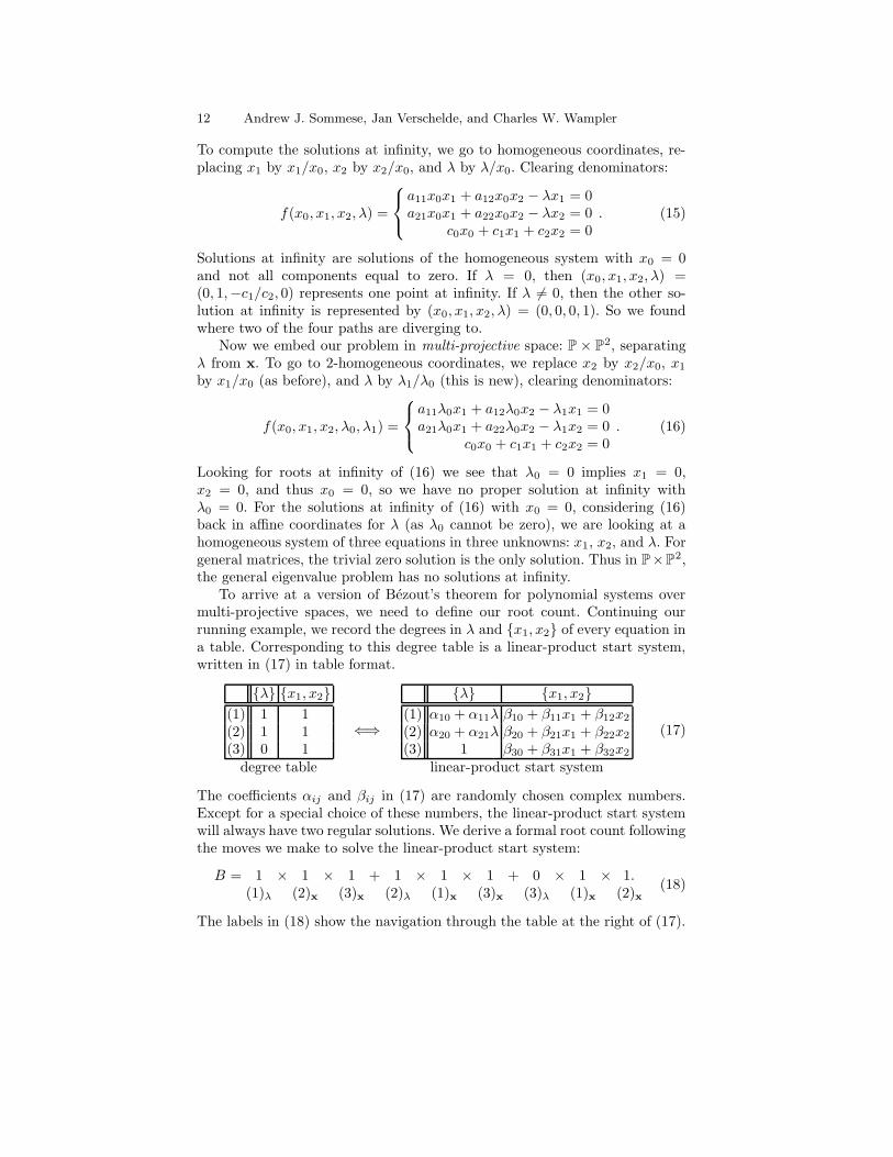
To arrive at a version of Bezout’s theorem for polynomial systems overmulti-projective spaces, we need to define our root count. Continuing ourrunning example, we record the degrees in λ and {x1, x2} of every equation ina table. Corresponding to this degree table is a linear-product start system,written in (17) in table format.

{λ} {x1, x2}(1) 1 1(2) 1 1(3) 0 1degree table

⇐⇒

{λ} {x1, x2}(1) α10 + α11λ β10 + β11x1 + β12x2

(2) α20 + α21λ β20 + β21x1 + β22x2

(3) 1 β30 + β31x1 + β32x2

linear-product start system

(17)

The coefficients αij and βij in (17) are randomly chosen complex numbers.Except for a special choice of these numbers, the linear-product start systemwill always have two regular solutions. We derive a formal root count followingthe moves we make to solve the linear-product start system:

B = 1 × 1 × 1 + 1 × 1 × 1 + 0 × 1 × 1.(1)λ (2)x (3)x (2)λ (1)x (3)x (3)λ (1)x (2)x

(18)

The labels in (18) show the navigation through the table at the right of (17).


Exercise 4. The matrix polynomial

p(λ) = Adλd +Ad−1λ

d−1 + · · ·+A1λ+A0, Ai ∈ Cn×n, (19)

defines the generalized eigenvalue problem p(λ)x = 0. How many generalizedeigenvalue-eigenvector pairs can we expect for randomly chosen matrices Ai?

To show that B is an upper bound for the number of isolated solutions ofa polynomial system, we show the regularity and boundedness of the solutionpaths in a typical homotopy, using a linear-product start system.

For many applications (like the eigenvalue problem) it is obvious how bestto separate the variables into a partition. But for blackbox solvers and systemswith no apparent product structure, we need to find that partition which leadsto the smallest Bezout number. One strategy is to enumerate all partitionsand retain the partition with the smallest Bezout number. While the numberof partitions grows faster than 2n, finding the smallest Bezout number forn = 8 by enumeration takes less than a second of CPU time.

Instead of using one partition of the variables to model the product struc-ture of the system, we may use different partitions for different equations,and extend this even further to construct in this way general linear-productstart systems. The solving of the start system now involves more work, butwe may expect the homotopy to be more efficient. Schematically, a hierarchyof homotopies (and root counting methods) is given in Figure 4.

Coefficient-Parameter

NewtonPolytopes

PolynomialProducts

Linear Products

Multihomogeneous

Total Degree

�

�

�

�

�

�

easierstartsystem

?

more efficient(fewer paths)

6iA

Fig. 4. A hierarchy of homotopies. All homotopies below the dashed line A can bedone automatically. Above the line, apply special ad-hoc methods or bootstrapping.Homotopies at the bottom of the hierarchy are often used to find solutions for genericinstances of parameters in a coefficient-parameter homotopy.

Wewill not address the “polynomial products” of Figure 4 here, see [MSW95].We introduce the Newton polytopes in the following two sections.


3.4 Polyhedral Homotopies to glue Real Solutions

The purpose of this section is to introduce Newton polytopes and polyhedralhomotopies, but without mixed volumes. So we restrict ourselves to polyno-mials in one variable. Instead of “just” solving a polynomial in one variable,we consider a different problem:

Input: k distinct monomials in one variable x:xa1 , xa2 , . . . , xak , with ai 6= aj for i 6= j.

Output: coefficients ca1 , ca2 , . . . , caksuch that

f(x) = ca1xa1 + ca2x

a2 + · · ·+ cakxak

has k − 1 positive real roots.

For example, take 1, x5, x7, x11 as monomials on input. Then the problem isto find c0, c5, c7, and c11 such that f(x) = c01+c5x

5+c7x7+c11x

11 has threepositive real solutions. We will show that we can reduce this four dimensionalproblem in that of one dimension, considering the homotopy

h(x, t) = t− x5 + x7 − x11t = 0, for t ≥ 0. (20)

The alternation of signs in the coefficients is a deliberate choice to maximizethe number of positive real roots. The Newton polytope of a polynomial isthe convex hull of the exponent vectors of those monomials appearing witha nonzero coefficient. The choice of powers of t with each monomial is suchthat the lower hull of the Newton polytope of h contains among its verticesall exponents of the given monomials, see Figure 5.

t(0,1)

``````````t(5,0) t(7,0)»»»»»»

»»t(11,1)

Fig. 5. The Newton polytope of the homotopy h(x, t) = 0 is spanned by by theexponent vectors of the monomials in h. The lower hull of the Newton polytopes isdrawn in solid lines.

At t = 0, the homotopy h(x, 0) = −x5 + x7 = x5(−1 + x2) = 0 has onepositive real root: x = 1. The idea is to choose t = ∆t > 0 such that Newton’smethod applied to h(x,∆t) = 0 converges quadratically to a positive real rootstarting at x = 1. (Notice that by the fortunate choice of the powers of t inthe example, ∆t can be chosen arbitrarily large as h(1, t) ≡ 0, for any valueof t.)

Observe that the monomials in h(x, 0) correspond to the lowest middleedge on the lower hull of the Newton polytope of h in Figure 5. For everyedge of the lower hull of the Newton polytope we will use one homotopy tofind one positive real root. Each time, the start system in the homotopy has itstwo monomials as vertices of an edge of the lower hull. To find the homotopies


with the other two edges, we need to consider the vectors orthogonal to theedges (we call those vectors inner normals), see Figure 6.

t(0,1)

``````````t(5,0) t(7,0)»»»»»»

»»t(11,1)

¥¥º

v1

6

v2

CCO

v3

Fig. 6. Inner normals v1 = ( 15, 1), v2 = (0, 1), v3 = (− 1

4, 1) on the edges of the

lower hull of the Newton polytope of the homotopy h(x, t) = 0.

The inner normal v1 attains the minimal inner product with those verticeson the first edge of the lower hull. Consider the four values of the inner productof v1 with the four vertices of the lower hull:

〈(1

5, 1

), {(0, 1), (5, 0), (7, 0), (11, 1)}〉=

{1, 1,

7

5,16

5

}. (21)

Indeed, the minimal values occur with the first two vertices which span thefirst edge. This geometric construction motivates the following change of co-ordinates: let x = yt1/5, we obtain

h(y, t) = t− y5t+ y7t7/5 − y11t16/5 (22)

= t(1− y5 + y7t2/5 − y11t11/5

). (23)

We see that 1th(y, 0) = 1− y5 = 0 has one positive real root: y = 1. Now we

can choose t = ∆t > 0 such that Newton’s method converges quadratically toa positive real root starting at y = 1. Let y∗: h(y∗, ∆t) = 0, then we find thecorresponding root in the original coordinates as x∗ = y∗(∆t)1/5.

We can even explicitly construct the fractional power series using Newton’smethod in a computer algebra system like Maple. The following sequence ofMaple commands achieve this:

> h := t-x^5 + x^7 - x^(11)*t:

> hy := subs(x = y*t^(1/5),h):

> hyt := simplify(hy/t):

> newton := x -> x - subs(y=x,hyt/diff(hyt,y)):

> x[0] := 1:

> for k from 1 to 6 do

> x[k] := newton(x[k-1]):

> s[k] := series(x[k],t=0,15):

> lprint(op(1,s[k]-s[k-1]));

> end do:

The output of the loop (done in Maple 9) shows the errors between twoconsecutive series expansions:


1

-301/15625*t^2

-84/3125*t^2

-2112/1953125*t^(18/5)

-32768/152587890625*t^(32/5)

-2147483648/23283064365386962890625*t^(64/5)

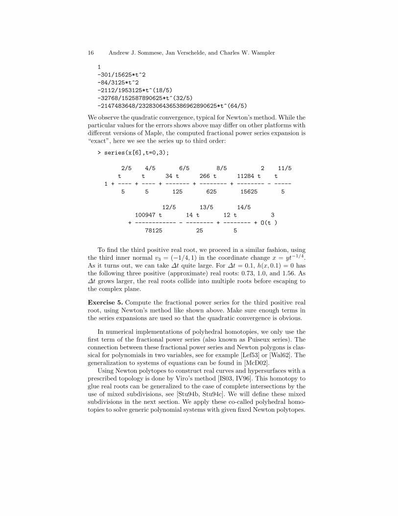
We observe the quadratic convergence, typical for Newton’s method. While theparticular values for the errors shows above may differ on other platforms withdifferent versions of Maple, the computed fractional power series expansion is“exact”, here we see the series up to third order:

> series(x[6],t=0,3);

2/5 4/5 6/5 8/5 2 11/5

t t 34 t 266 t 11284 t t

1 + ---- + ---- + ------- + -------- + -------- - -----

5 5 125 625 15625 5

12/5 13/5 14/5

100947 t 14 t 12 t 3

+ ------------ - -------- + -------- + O(t )

78125 25 5

To find the third positive real root, we proceed in a similar fashion, usingthe third inner normal v3 = (−1/4, 1) in the coordinate change x = yt−1/4.As it turns out, we can take ∆t quite large. For ∆t = 0.1, h(x, 0.1) = 0 hasthe following three positive (approximate) real roots: 0.73, 1.0, and 1.56. As∆t grows larger, the real roots collide into multiple roots before escaping tothe complex plane.

Exercise 5. Compute the fractional power series for the third positive realroot, using Newton’s method like shown above. Make sure enough terms inthe series expansions are used so that the quadratic convergence is obvious.

In numerical implementations of polyhedral homotopies, we only use thefirst term of the fractional power series (also known as Puiseux series). Theconnection between these fractional power series and Newton polygons is clas-sical for polynomials in two variables, see for example [Lef53] or [Wal62]. Thegeneralization to systems of equations can be found in [McD02].

Using Newton polytopes to construct real curves and hypersurfaces with aprescribed topology is done by Viro’s method [IS03, IV96]. This homotopy toglue real roots can be generalized to the case of complete intersections by theuse of mixed subdivisions, see [Stu94b, Stu94c]. We will define these mixedsubdivisions in the next section. We apply these co-called polyhedral homo-topies to solve generic polynomial systems with given fixed Newton polytopes.


3.5 The Cayley trick and Minkowski’s theorem

Mixed volumes were defined by Minkowski who showed that the volume of alinear combination of polytopes is a homogeneous polynomial in the factorsof of the combination. The coefficients of this polynomial are mixed volumes.We will visualize this theorem on a simple example by the Cayley trick.

The Cayley trick [GKZ94, Proposition 1.7, page 274] is a method to rewritea certain resultant as a discriminant of one single polynomial with additionalvariables. The polyhedral version of this trick as in [Stu94a, Lemma 5.2] isdue to Bernd Sturmfels. See [HRS00] for another application of this trick.

Consider the following system:

f = (f1, f2)

=

{x3

1x2 + x1x22 + 1 = 0

x41 + x1x2 + 1 = 0

A = (A1, A2)A1 = {(3, 1), (1, 2), (0, 0)}A2 = {(4, 0), (1, 1), (0, 0)}

(24)

The sparse structure of f is modeled by the tuple A = (A1, A2), where A1

and A2 are the supports of f1 and f2 respectively. The Newton polytopes arethe convex hulls of the supports. The Cayley polytope of r polytopes is theconvex hull of the polytopes placed at the vertices of an (r − 1)-dimensionalunit simplex. Figure 7 illustrates this construction for our example.

(3,1,0) (1,2,0)

(0,0,0)

(4,0,1) (1,1,1)

(0,0,1)

(3,1,0) (1,2,0)

(0,0,0)

(4,0,1) (1,1,1)

(0,0,1)

Fig. 7. The Cayley polytope of two polygons. The first polygon is placed at thevertex (0, 0, 0), the second polygon is placed at (0, 0, 1).

For our example, the Cayley polytope is so simple that a triangulation isobvious (see Figure 8). As every simplex has four vertices, either the simplexhas three vertices from the same polygon (and the fourth one of the otherpolygon), or the simplex has two vertices of each polygon. A simplex of thefirst type is called unmixed, a simplex of the second type is mixed. Imaginetaking slices parallel to the base of the Cayley polytope. These slices producescaled copies of the original polygons in the unmixed simplices. In the mixed


simplex we find one scaled edge from the first and another scaled edge fromthe second polygon, see Figure 8.

(3,1,0) (1,2,0)

(0,0,0)

(4,0,1)

(1,2,0)

(4,0,1) (1,1,1)

(0,0,1)

(1,2,0)

(0,0,0)

(4,0,1)

(0,0,1)

Fig. 8. A triangulation of the Cayley polytope. The middle simplex is mixed, theother two simplices are unmixed.

On Figure 9 we see in the cross section of the Cayley polytope a mixedsubdivision of the convex combination λ1P1 + λ2P2, λ1 + λ2 = 1, λ1 ≥ 0 andλ2 ≥ 0, where P1 defines the base and P2 is at the top of the polytope. Theareas of the triangles in the cross section are λ2

1×area(P1) and λ22×area(P2),

as each side of the triangle is scaled by λ1 and λ2 respectively. The area of thecell in the subdivision spanned by one edge of P1 (scaled by λ1) and the otheredge of P2 (scaled by λ2) is scaled by λ1 × λ2, as we move the cross section.

(3,1,0) (1,2,0)

(0,0,0)

(4,0,1) (1,1,1)

(0,0,1)

(3,1,0)(1,2,0)

(0,0,0)

Fig. 9. A mixed subdivision induced by a triangulation of the Cayley polytope.

In Figure 10 we show the Minkowski sum of the two polygons P1 and P2,with their mixed subdivision corresponding to the triangulation of the Cayleypolytope. For this example, Minkowski’s theorem becomes


area(λ1P1 + λ2P2)=V (P1, P1)λ21 + V (P1, P2)λ1λ2 + V (P2, P2)λ

22

=3λ21 + 8λ1λ2 + 2λ2

2.(25)

The coefficients in the polynomial (25) are mixed volumes (or areas in ourexample): V (P1, P1) and V (P2, P2) are the respective areas of P1 and P2,while V (P1, P2) is the mixed area.

s(0,0)

s(1,2)

s(3,1)

qqqqqqqqqq

q q q q q q q q q qq q q qq q q q q q q q q qP1

s(0,0)

s(1,1)

s(4,0)

¡¡PPPPPP2 s

(0,0)+(0,0)

s(0,0)+(1,2)

s(0,0)+(4,0)

s(1,2)+(4,0)

s(1,2)+(1,1)

s(3,1)+(4,0)qqqq

qqqqqq

qqqqqqqqqq

q q q q q q q q q qq q q qq q q q q q q q q q

¡¡PPPPP

λ1λ2

λ22

λ21

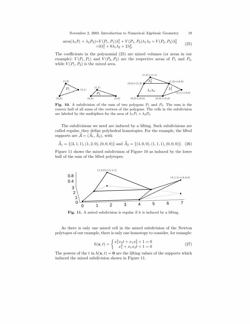
Fig. 10. A subdivision of the sum of two polygons P1 and P2. The sum is theconvex hull of all sums of the vertices of the polygons. The cells in the subdivisionare labeled by the multipliers for the area of λ1P1 + λ2P2.

The subdivisions we need are induced by a lifting. Such subdivisions arecalled regular, they define polyhedral homotopies. For the example, the liftedsupports are A = (A1, A2), with

A1 = {(3, 1, 1), (1, 2, 0), (0, 0, 0)} and A2 = {(4, 0, 0), (1, 1, 1), (0, 0, 0)}. (26)

Figure 11 shows the mixed subdivision of Figure 10 as induced by the lowerhull of the sum of the lifted polytopes.

0 1 2 3 4 5 6 701

23

0.40.8

(1,2,0)+(1,1,1)

(3,1,1)+(4,0,0)

Fig. 11. A mixed subdivision is regular if it is induced by a lifting.

As there is only one mixed cell in the mixed subdivision of the Newtonpolytopes of our example, there is only one homotopy to consider, for example:

h(x, t) =

{x3

1x2t+ x1x22 + 1 = 0

x41 + x1x2t+ 1 = 0

(27)

The powers of the t in h(x, t) = 0 are the lifting values of the supports whichinduced the mixed subdivision shown in Figure 11.


Exercise 6. Verify that the start system h(x, t = 0) = 0 in the polyhedralhomotopy (27) has indeed eight (= V (P1, P2)) regular solutions. Show thatany system with exactly two monomials in every equation has always as manyregular roots as its mixed volume, for any nonzero choice of the coefficients.

3.6 Computing Mixed Volumes and Polyhedral Continuation

In the previous subsections we introduced polyhedral continuation and mixedvolumes. With these two concepts we can state and prove Bernshteın’s firsttheorem. As the way we compute mixed volumes determines the way we solve ageneric system, this section presents two different methods to compute mixedvolumes. The first technique relies on the Cayley trick and computes all cellsin a mixed subdivision. The second method uses linear programming and leadsto an efficient enumeration of all mixed cells in a mixed subdivision.

With the Cayley trick we can obtain a regular mixed subdivision as aregular triangulation of the Cayley polytope. We next introduce a method tocompute a regular triangulation of any polytope. Our method will constructthe triangulation incrementally, adding the points one after the other. The keyoperation is to decompose one point with respect to one simplex. Considerfor example the simplex [c0, c1, c2] spanned by c0 = (0, 0), c1 = (3, 2), andc2 = (2, 4). If we take one extra point, three possible updates can occur,illustrated by Table 2.

point barycentric decomposition pivoting

x = (2, 3): x = + 18

c0 + 14

c1 + 58

c2 no new simplex

y = (5, 1): y = − 13

c0 + 94

c1 −78

c2 [y, c1, c2][c0, c1,y]

z = (1, 5): z = + 18

c0 −34

c1 + 138

c2 [c0, z, c2]

Table 2. Three possible updates of the simplex [c0, c1, c2] with one point, x, y,or z. Either we have no, two, or one new simplex by interchanging the vertex withnegative coefficient with the point.

Solving a linear system we can write any point as a linear combination ofthe vertices of a simplex, requiring the coefficients in that linear combinationto sum up to one. We call this linear combination a barycentric decomposi-tion of a point with respect to a simplex. The negative signs of the coefficientsin this barycentric decomposition tell which vertices of the simplex to inter-change with the new point to create new simplices in the triangulation of theconvex hull of the original simplex and the point. As we can see from Fig-


0

1

2

3

4

5

1 2 3 4 50

1

2

3

4

5

0

1

2

3

4

5

0

0.5

1

1.5

x

c0

y

c1

z

c2(z, 1)

(y, 1)

Fig. 12. Pivoting to obtain a regular triangulation of a polygon. The constructionon the right shows how the triangulation can be obtained as the lower hull of y andz lifted at height one, with [c0, c1, c2] sitting at level zero.

ure 12, any triangulation obtained by placing points (see [Lee91] for more ontriangulations) in this way is regular.

The algorithm to compute regular triangulations incrementally leads toan incremental polyhedral solver, which solves polynomial systems adding onemonomial after the other, see [VGC96]. If the structure of a polynomial systemis such that most polynomials share the same support (or more generally spanthe same Newton polytope), and thus there are only few distinct Newtonpolytopes to consider, then the Cayley trick is not too wasteful.

The complexity of computing volumes and mixed volumes is discussedrespectively in [DF88] and [DGH98].

Theorem 2. (Bernshteın’s theorem A) The number of roots of a generic

system equals the mixed volume of its Newton polytopes.

In his proof of this theorem, Bernshteın [Ber75] used a homotopy (imple-mented in [VVC94]), based on a recursive formula for computing mixed vol-umes. This proof idea was generalized by Huber and Sturmfels in [HS95].Note that the theorem concerns “generic systems”, which are systems withrandomly chosen coefficients. These generic systems serve as start system in acoefficient-parameter homotopy to solve any specific polynomial system withthe same Newton polytopes.

For the coordinate changes in the polyhedral homotopies, we need to knowthe inner normals to the mixed cells. Therefore, we use a dual representationof polytopes, see Figure 13. The normal fan of a polytope is the collectionof the normal cones to all faces of the polytope. The normal cone to a facecontains all inner normals which define the face.


s(0,0)

s(1,2)

s(3,1)

qqqqqqqqqq

q q q q q q q q q qq q q qq q q q q q q q q qP1

sqqqqqqqq(−1,3)

q q q q q q q q(2,−1)

qqqqqqqqqq(−1,−2)

N (P1)

s(0,0)

s(1,1)

s(4,0)

¡¡PPPPPP2

s

(0,1)

@@@(1,−1)

£££

(−1,−3)

N (P2)

Fig. 13. Two polygons P1 and P2 and their normal fans, N (P1) and N (P2). Thelabels corresponding to the edges in the fans are inner normals to the correspondingedges of the polygons.

We are only interested in the mixed cells of a mixed subdivision, and inparticular, the inner normal to those lower facets of the Minkowski sum whichdefine the mixed cells. Figure 14 illustrates that the inner normal to a mixedcell lies in the intersection of the normal cones to the edges which span thatmixed cell.

s

s

s

ss

sqqqqqqqqqq

qqqqqqqqqq

q q q q q q q q q qq q q qq q q q q q q q q q

¡¡

PPPPP sqqqqqqqqq q q q q q q qqqqqqqqqqqs@@@

£££

Fig. 14. The dual representation of a mixed subdivision.

The search for all inner normals to the mixed cells in a mixed subdivisionnaturally leads to a system of linear equalities and inequalities. For a tuple ofn supports (A1, A2, . . . , An), consider an edge of the kth polytope, spannedby {a,b} ⊆ Ak . Then the inner normal v to this edge satisfies

{〈a,v〉 = 〈b,v〉〈a,v〉 ≤ 〈c,v〉, for all c ∈ Ak.

(28)

Enumerating all edges of a polytope is thus equivalent to enumerating all fea-sible solutions to the system (28). Letting k range from 1 to n in (28) applied

to the lifted point sets Ak provides the dual linear-programming model toenumerate all inner normals to the mixed cells in a regular mixed subdivision.

A lift-and-prune strategy to enumerate all mixed cells in a regular mixedsubdivision was proposed in [EC95] and dualized in [VGC96]. Recently, in-sight in the linear programming methods has led to very efficient calculationsof mixed volumes, as developed in [DKK03], [GL00, GL03], [KK03], [LL01],and [TKF02].


3.7 Bernshteın’s Second Theorem

When tracing solution paths diverging to infinity, one may wonder when tostop. After all, infinity is pretty far off, and even if good knowledge of theapplication domain gives us good bounds on the size of the solutions, we donot want to miss valid solutions with large components. If a path seems todiverge, we must know whether we have true divergence or convergence to aroot with large components. Bernshteın’s second theorem [Ber75] will provideus with a certificate of divergence.

For a system f(x) = 0, supported by A = (A1, A2, . . . , An), we can writeits equations f = (f1, f2, . . . , fn) as

fi(x) =∑

a∈Ai

ciaxa, i = 1, 2, . . . , n. (29)

The Newton polytopes of f are denoted by P = (P1, P2, . . . , Pn), with Pi :=conv(Ai), i = 1, 2, . . . , n. Then for any ω 6= 0, we define the tuple of faces∂ωP = (∂ωP1, ∂ωP2, . . . , ∂ωPn), as ∂ωPi := conv(∂ωAi), with

∂ωAi := { a ∈ Ai | 〈a, ω〉 = mina′∈Ai

〈a′, ω〉 }. (30)

The set ∂ωAi is the support of the face of the ith polynomial fi:

∂ωfi(x) =∑

a∈∂ωAi

ciaxa. (31)

We write ∂ωf = (∂ωf1, ∂ωf2, . . . , ∂ωfn) as the face of the system f determinedby ω 6= 0. The mixed volume of P is denoted by V (P) and C∗ = C \ {0}.

Theorem 3. (Bernshteın’s theorem B) If ∀ω 6= 0, ∂ωf(x) = 0 has no so-

lutions in (C∗)n, then V (P) is exact and all solutions are isolated. Otherwise,for V (P) 6= 0: V (P) > #isolated solutions.

Interestingly, the Newton polytopes may often be in general position, i.e.:V (P) is exact for every nonzero choice of the coefficients. Consider for examplethe following system:

f(x) =

{c111x1x2 + c110x1 + c101x2 + c100 = 0

c222x21x

22 + c210x1 + c201x2 = 0

(32)

We show the tuple of Newton polytopes in Figure 15.

Exercise 7. Verify that the mixed volume V (P1, P2) of the polygons P1 andP2 is indeed equal to four.

While the observation in Figure 15 would let us believe that the mixedvolume always provides a sharp root count, we have to keep in mind thatthe vertices of the polytopes are not randomly chosen. The vertices occur as


t(0,0)

t(0,1) t(1,1)

t(1,0)

P1t

(1,0)

t(0,1)

t(2,2)

¢¢

¢¢

@@

©©©©

P2

Fig. 15. Two Newton polygons in general position: ∀ω 6= 0 : ∂ωA1 + ∂ωA2 ≤ 3 ⇒V (P1, P2) = 4 is always exact, for all nonzero choices of the coefficients of f , becausewe need at least four monomials for ∂ωf(x) = 0 to have all its roots in ( � ∗ )2.

the exponents in the polynomials. For instance, general Newton polytopes arealmost never simplicial, we usually find k-dimensional faces spanned by farmore than k + 1 vertices.

Following Bernshteın we look at what happens when we consider the solu-tion paths in a homotopy going from a generic to a specific polynomial system.At the limit of the paths, we look at the power series expansion, using thefollowing result.

Theorem 4. ∀x(t), h(x(t), t) = (1− t)g(x(t)) + tf(x(t)) = 0,

∃s > 0, m ∈ N \ {0}, ω ∈ Zn:

{xi(s) = bis

ωi(1 +O(s)), i = 1, 2, . . . , nt(s) = 1− sm for t ≈ 1, s ≈ 0

The number m is called the winding number of the solution at the end ofthe path (not to be confused with the multiplicity). The winding number isthe smallest number so that z(2πm) = z(0), if we consider z(θ) a solutionpath of h(z(θ), t(θ)) = 0, winding around 1 with values for the continuationparameter t defined by t = 1 + (t0 − 1)eiθ, as t0 ≈ 1.

At the end of a path, when does limt→1

xi(t) ∈ C∗? From Theorem 4, we can

characterize the divergence of the path x(t) by the leading exponents ω in thepower series:

xi(t)

→∞∈ C∗

→ 0⇔ ωi

< 0= 0> 0

(33)

From this simple observation we see that a solution at infinity and a solutionwith zero components are regarded (or disregarded) equally.

Next we show the relation between face systems and power series. Assum-ing lim

t→1xi(t) 6∈ C∗, and ωi 6= 0, we consider a diverging path.

First we substitute the power series xi(s) = bisωi(1+O(s)), i = 1, 2, . . . , n,

t(s) = 1− sm, s ≈ 0 into the homotopy h(x, t) = (1− t)g(x) + tf(x) = 0. Wefind

h(x(s), t(s)) = f(x(s))︸︷︷︸dominant as s→0

+sm(g(x(s)) − f(x(s))) = 0. (34)

Thus (as expected), the choice of the start system g(x) = 0 plays no role inwhat happens as s approaches zero. Let us now see what the substitution does


to the ith polynomial:

fi(x) =∑

a∈Ai

ciaxa → fi(x(s)) =

∑

a∈Ai

cia

n∏

i=1

bai

i s〈a,ω〉(1

︸︷︷︸∂ωfi(x(s)) dominant

+O(s)). (35)

Arranging the monomials in f(x(s)) in increasing order of powers of s, we seethat the monomials that become dominant as s → 0 have exponents whoseinner product is minimal with ω. Recall that we characterize these exponentsby the face of the support Ai in the direction of ω, see (30). Moreover, asfi(x(s)) = 0 for s → 0, we see from the result of the substitution that then∂ωfi(b) = 0, and thus ∂ωf(b) = 0 for some b ∈ (C∗)n.

This is the key idea in the proof of Bernshteın’s second theorem. Like hisfirst theorem, his idea is very constructive: follow the direction of a divergingpath and (in addition to a solution at infinity) we find a face system which hassolutions in (C∗)n. This face system forms a certificate for the mixed volumeto overshoot the actual number of roots.

That Richardson extrapolation is useful to find ω is not so surprising. Acloser inspection of the errors of the error expansion reveals that a similarextrapolation scheme can be applied to approximate the winding number m.

As we get closer to our target system, we have to decrease our step sizewhen dealing with a difficult path. For the purpose of extrapolation, we betterdecrease the step size geometrically, i.e., for some λ, 0 < λ < 1, consecutivevalues t0, t1, . . . tk of the continuation parameter t satisfy 1− tk = λ(1− tk) =· · · = λk(1 − t0) and for the corresponding sequence of s-values we havesk = λ1/msk−1 = · · · = λk/ms0.

Recall the form of the power series for a solution path x(s) for s ap-proaching zero: xi(s) = bis

ωi(1 + O(s)) with t(s) = 1 − sm. Sampled alongs0, s1, . . . , sk, we obtain

xi(sk) = biλkωi/msωi

0 (1 +O(λk/ms0)). (36)

Since we are interested in the leading powers ωi, we take the logarithms ofthe magnitudes of the points sampled along the path:

log |xi(sk)| = log |bi|+kωim

log(λ) + ωi log(s0) + log

∣∣∣∣∣∣1 +

∞∑

j=0

b′j(λk/ms0)

j

∣∣∣∣∣∣.

(37)A first-order approximation for ωi is given by vkk+1 with the general extrap-olation formula in vk..l:

vkk+1 := log |xi(sk+1)|− log |xi(sk)|, vk..l = vk..l−1+vk+1..l − vk..l−1

1− λ(38)

which results in ωi = m v0..r

log(λ) + O(sr0). While we can make the order r of

the extrapolation as high as we like (thereby increasing the accuracy of ωi).Notice that the formula assumes we know the winding number m.


If we examine the expansion of the errors:

e(k)i = (log |xi(sk)| − log |xi(sk+1)|) (39)

−(log |xi(sk+1)| − log |xi(sk+2)|) (40)

= c1λk/ms0(1 + 0(λk/m)), (41)

we find similar extrapolation formulas to approximate m:

e(kk+1)i := log(e

(k+1)i )− log(e

(k)i ), e

(k..l)i = e

(k+1..l)i +

e(k..l−1)i − e

(k+1..l)i

1− λk..l(42)

with λk..l = λ(l−k−1)/mk..l . So we obtain mk..l =log(λ)

e(k..l)i

+O(λ(l−k)k/m)

The system of Cassou-Nogues is a very nice example. It illustrates howsymbolic results can be obtained by purely numerical means.

f(b, c, d, e) =

15b4cd2 + 6b4c3 + 21b4c2d− 144b2c− 8b2c2e−28b2cde− 648b2d+ 36b2d2e+ 9b4d3 − 120 = 0

30c3b4d− 32de2c− 720db2c− 24c3b2e− 432c2b2 + 576ec−576de+ 16cb2d2e+ 16d2e2 + 16e2c2 + 9c4b4 + 5184

+39d2b4c2 + 18d3b4c− 432d2b2 + 24d3b2e− 16c2b2de− 240c = 0216db2c− 162d2b2 − 81c2b2 + 5184 + 1008ec− 1008de

+15c2b2de− 15c3b2e− 80de2c+ 40d2e2 + 40e2c2 = 0261 + 4db2c− 3d2b2 − 4c2b2 + 22ec− 22de = 0

(43)

Root counts: D = 1344, B = 312, V (P) = 24, but there are only 16 finiteroots.

∂(0,0,0,−1)f(b, c, d, e) =

−8b2c2e− 28b2cde+ 36b2d2e = 0−32de2c+ 16d2e2 + 16e2c2 = 0−80de2c+ 40d2e2 + 40e2c2 = 0

22ec− 22de = 0

(44)

The winding number is m = 2. See [HV98] for more about polyhedral endgames.

4 Homotopies for Positive Dimensional Solution Sets

To introduce the numerical representation of positive dimensional solutionsets, we start off with a dictionary, linking concepts in algebraic geometryto data and algorithms in numerical analysis. Witness sets form the centraldata and are obtained by a cascade of homotopies. The companion algorithmsto the witness sets are membership tests to decide whether any given pointbelongs to a certain component of the solution set. We illustrate a numericalirreducible decomposition on a simple example and give an overview of ournumerical factorization methods.


4.1 A Dictionary

Kempf writes in [Kem93] that “Algebraic geometry studies the delicate bal-ance between the geometrically plausible and the algebraically possible”. Withour numerical tools, we feel closer to the geometrical than to the algebraicside, because we are not calculating with polynomials in the algebraic sense.In [SVW03c] we outlined the structure of a dictionary, presented as Table 3.

Numerical Algebraic Geometry Dictionary

Algebraic example NumericalGeometry in 3-space Analysis

variety collection of points, polynomial systemalgebraic curves, and + union of witness sets, see belowalgebraic surfaces for the definition of a witness point

irreducible a single point, or polynomial systemvariety a single curve, or + witness set

a single surface + probability-one membership test

generic point random point on point in a witness set; a witness pointon an an algebraic is a solution of the polynomial system on

irreducible curve or surface the variety and on a random slice whosevariety codimension is the dimension of the variety

pure one or more points, or polynomial systemdimensional one or more curves, or + set of witness sets of same dimension

variety one or more surfaces + probability-one membership tests

irreducible several pieces polynomial systemdecomposition of different + array of sets of witness sets andof a variety dimensions probability-one membership tests

Table 3. Dictionary to translate algebraic geometry into numerical analysis.

4.2 Witness Sets and a Cascade of Homotopies

A witness set is the basic concept of numerical algebraic geometry as it allowsus to apply numerical methods for isolated solutions to positive dimensionalsolution components.

Every irreducible component of a solution set is presented by a witness setwhose cardinality equals the degree of the irreducible component. To reducea solution set of dimension k to a set of isolated points, we cut the k degreesof freedom by adding k random hyperplanes L(x) = 0 to the system f(x) = 0which defines the entire solution set.

One obstacle is that we have to deal with systems whose number of equa-tions in not necessarily the same as the number of unknowns. If there arefewer equations than unknowns, we simply add enough random hyperplanesto make up for the difference, so underdetermined systems are easy to handle.


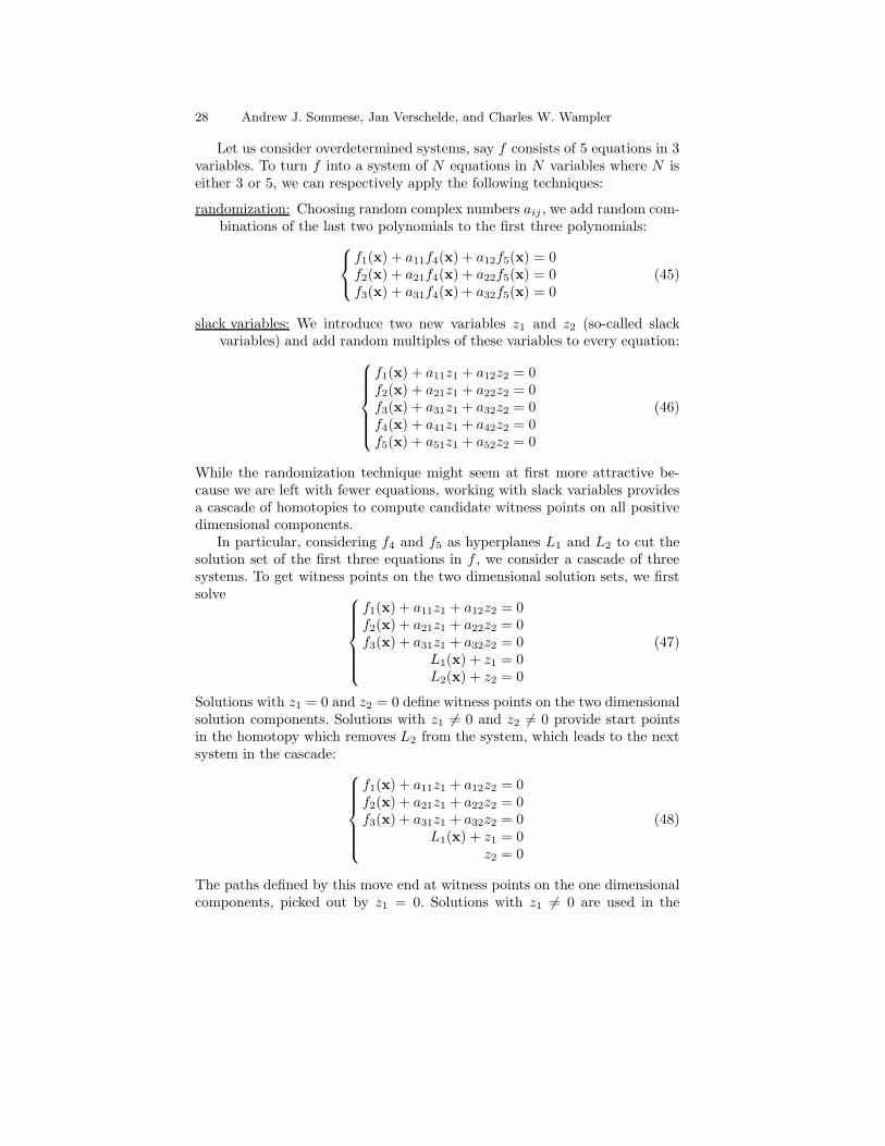
Let us consider overdetermined systems, say f consists of 5 equations in 3variables. To turn f into a system of N equations in N variables where N iseither 3 or 5, we can respectively apply the following techniques:

randomization: Choosing random complex numbers aij , we add random com-binations of the last two polynomials to the first three polynomials:

f1(x) + a11f4(x) + a12f5(x) = 0f2(x) + a21f4(x) + a22f5(x) = 0f3(x) + a31f4(x) + a32f5(x) = 0

(45)

slack variables: We introduce two new variables z1 and z2 (so-called slackvariables) and add random multiples of these variables to every equation:

f1(x) + a11z1 + a12z2 = 0f2(x) + a21z1 + a22z2 = 0f3(x) + a31z1 + a32z2 = 0f4(x) + a41z1 + a42z2 = 0f5(x) + a51z1 + a52z2 = 0

(46)

While the randomization technique might seem at first more attractive be-cause we are left with fewer equations, working with slack variables providesa cascade of homotopies to compute candidate witness points on all positivedimensional components.

In particular, considering f4 and f5 as hyperplanes L1 and L2 to cut thesolution set of the first three equations in f , we consider a cascade of threesystems. To get witness points on the two dimensional solution sets, we firstsolve

f1(x) + a11z1 + a12z2 = 0f2(x) + a21z1 + a22z2 = 0f3(x) + a31z1 + a32z2 = 0

L1(x) + z1 = 0L2(x) + z2 = 0

(47)

Solutions with z1 = 0 and z2 = 0 define witness points on the two dimensionalsolution components. Solutions with z1 6= 0 and z2 6= 0 provide start pointsin the homotopy which removes L2 from the system, which leads to the nextsystem in the cascade:

f1(x) + a11z1 + a12z2 = 0f2(x) + a21z1 + a22z2 = 0f3(x) + a31z1 + a32z2 = 0

L1(x) + z1 = 0z2 = 0

(48)

The paths defined by this move end at witness points on the one dimensionalcomponents, picked out by z1 = 0. Solutions with z1 6= 0 are used in the


homotopy which removes L1 to lead to the isolated solutions of the system.The last system in the cascade is

f1(x) + a11z1 = 0f2(x) + a21z1 = 0f3(x) + a31z1 = 0

z1 = 0z2 = 0

(49)

In the next section we give a specific example of this cascade.The idea of slicing a solution set by hyperplanes to determine its dimension

appeared in [GH93] to prove that the theoretical complexity of this problemis polynomial.

Exercise 8. Consider the adjacent minors of a general 2× 4-matrix:

[x11 x12 x13 x14

x21 x22 x23 x24

]f(x) =

x11x22 − x21x12 = 0x12x23 − x22x13 = 0x13x24 − x23x14 = 0

(50)

Verify that dim(f−1(0)) = 5 and deg(f−1(0)) = 8. This is the simplest in-stance of a general family of problems introduced in [DES98], see [HS00] forspecial decomposition methods.

4.3 A probability-one membership test

A probability-one membership test determines whether a given point p lieson a pure dimensional solution set. Suppose we have witness points definedby a polynomial system f(x) = 0 and hyperplanes L(x) = 0. A homotopymethod implements the probability-one membership test:

1. Define K(x) = L(x) − L(p). As K(p) = 0, the hyperplanes K passthrough p.

2. Consider the homotopy

h(x, t) =

(f(x)K(x)

)(1− t) +

(f(x)L(x)

)t = 0. (51)

At t = 1 we start tracking paths at the witness set and find their endpoints at t = 0.

3. If p belongs to the solution set of h(x, 0) = 0, then it is also a witnesspoint of the pure dimensional solution set.

Notice that this test does not move the point p, which may be a highly singularpoint. This observation is important for the numerical stability of this test.The test is illustrated in Figure 16.


L Kf−1(0)

sp 6∈ f−1(0)

Fig. 16. Illustration of a probability-one membership test using a homotopy. Thehomotopy moves the line L of the witness set for f−1(0) to the line K, which passesto the test point p. As none of the witness points on K equals p, p 6∈ f−1(0).

4.4 A Numerical Irreducible Decomposition

Consider the following example:

f(x) =

(x1 − 1)(x2 − x21) = 0

(x1 − 1)(x3 − x31) = 0

(x21 − 1)(x2 − x2

1) = 0(52)

From its factored form we see that f(x) = 0 has two solution components: thetwo dimensional plane x1 = 1 and the twisted cubic { (x1, x2, x3) | x2 − x2

1 =0, x3 − x3

1 = 0 }.To describe the solution set of this system, we use a cascade of homotopies,

the chart in Figure 17 illustrates the flow of data for this example.Because the top dimensional component is of dimension two, we add two

random hyperplanes to the system and make it square again by adding twoslack variables z1 and z2:

e(x, z1, z2) =

(x1 − 1)(x2 − x21) + a11z1 + a12z2 = 0

(x1 − 1)(x3 − x31) + a21z1 + a22z2 = 0

(x21 − 1)(x2 − x2

1) + a31z1 + a32z2 = 0c10 + c11x1 + c12x2 + c13x3 + z1 = 0c20 + c21x1 + c22x2 + c23x3 + z2 = 0

(53)

where all constants aij , i = 1, 2, 3, j = 1, 2, and ckl, k = 1, 2, l = 0, 1, 2, 3 arerandomly chosen complex numbers. Observe that when z1 = 0 and z2 = 0 thesolutions to e(x, z1, z2) = 0 satisfy f(x) = 0. So if we solve e(x, z1, z2) = 0we will find a single witness point on the two dimensional solution componentx1 = 1 as a solution with z1 = 0 and z2 = 0. Using polyhedral homotopies,this requires the tracing of six solutions paths.


The embedding was proposed in [SV00] to find generic points on all positivedimensional solution components with a cascade of homotopies. In [SV00]it was proven that solutions with slack variables zi 6= 0 are regular and,moreover, that those solutions can be used as start solutions in a homotopyto find witness points on lower dimensional solution components. At each stageof the algorithm, we call solutions with nonzero slack variables nonsolutions.

In the solution of e(x, z1, z2) = 0, one path ended with z1 = 0 = z2, thefive other paths ended in regular solutions with z1 6= 0 and z2 6= 0. These five“nonsolutions” are start solutions for the next stage, which uses the homotopy

h2(x, z1, z2, t)

=

(x1 − 1)(x2 − x21) + a11z1 + a12z2 = 0

(x1 − 1)(x3 − x31) + a21z1 + a22z2 = 0

(x21 − 1)(x2 − x2

1) + a31z1 + a32z2 = 0c10 + c11x1 + c12x2 + c13x3 + z1 = 0

z2(1− t) + (c20 + c21x1 + c22x2 + c23x3 + z2)t = 0

(54)

where t goes from one to zero, replacing the last hyperplane with z2 = 0.Of the five paths, four of them converge to solutions with z1 = 0. Of thosefour solutions, one of them is found to lie on the two dimensional solutioncomponent x1 = 1, the other three are generic points on the twisted cubic. Asthere is one solution with z1 6= 0, we have one candidate left to use as a startpoint in the final stage, which searches for isolated solutions of f(x) = 0. Thehomotopy for this stage is

h1(x, z1, t) =

(x1 − 1)(x2 − x21) + a11z1 = 0

(x1 − 1)(x3 − x31) + a21z1 = 0

(x21 − 1)(x2 − x2

1) + a31z1 = 0z1(1− t) + (c10 + c11x1 + c12x2 + c13x3 + z1)t = 0

(55)

which as t goes from 1 to 0, replaces the last hyperplane z1 = 0. At t = 0, thesolution is found to lie on the twisted cubic, so there are no isolated solutions.

The calculations are summarized in Figure 17. The breakup into irre-ducibles will be explained in the next section.

4.5 Factorization Methods

A recent trend in computer algebra is the adaptation of symbolic methodsto deal with approximate input data, which leads to the use of hybrid meth-ods [CKW02]. One such problem is the factorization of multivariate poly-nomials, listed as a challenge in [Kal00]. Recent papers on this problem are[CGvH+01, CGKW02], [GR01, GR02], [HWSZ00], and [Sas01].

Monodromy to Partition Witness Point Sets

We can see whether a curve factors or not by looking at its plot in complexspace, i.e.: we consider the curve as a Riemann surface. Figure 18 was madewith Maple (see [CJ98] for instructions).


WitnessGenerate

Path following

WitnessClassify

Filter Points Breakup into

Irreducibles¶µ

³´Homotopy + Start Solutions

?

¶µ

³´Filter = ∅

?level

2

6 paths - 0 at infinity

1 solutions

5 nonsolutions

?

-�W2

1 to classify -W21 on x1 = 1 = W21

?

Append to Filter

level

1

5 paths - 0 at infinity

4 solutions

1 nonsolution

?

-�W1

1 on x1 = 1 =J1

3 to classify -W1

3 on cubic = W11

?

Append to Filter

level

0

1 path - 0 at infinity

1 solution -�W0

0 on x1 = 1

1 on cubic

� �

� = J0

Fig. 17. Numerical Irreducible Decomposition of a system whose solutions are the2-dimensional plane x1 = 1 and the twisted cubic. At level i, for i = 2, 1, 0, we filtercandidate witness sets

�Wi into junk sets Ji and witness sets Wi. The sets Wi are

partitioned into witness sets Wij for the irreducible components.

Looking at Figure 18, imagine a line which intersects the surface in threepoints. Taking one complete turn of the line around the vertical axis z = 0will cause the points to permute. For example, the point which was lowest willhave moved up, while another point will have come down. Such a permutationcan only happen if the corresponding algebraic curve is irreducible.

Based on this observation, we can decompose any pure dimensional setinto irreducible components. Our monodromy algorithm returns a partitionof the witness set for a pure dimensional component: points in the same subsetof the partition belong to the same irreducible component. Recall that witnesspoints are defined by a system f(x) = 0 and a set of hyperplanes L(x) = 0.With the homotopy


–2

0

2

Re(z)

–2 –1 0 1 2Im(z)

–1.5

–1

–0.5

0

0.5

1

1.5

Re(z^1/3)

Fig. 18. The Riemann surface of z3 − w = 0. The height of the surface is the realpart of w = z1/3, while the gray scale corresponds to the imaginary part of w = z1/3.Observe that a loop around the origin permutes the order of points.

hKL(x, t) = λ

(f(x)K(x)

)(1− t) +

(f(x)L(x)

)t = 0, λ ∈ C, (56)

we find new witness points on the hyperplanes K(x) = 0, starting at thosewitness points satisfying L(x) = 0, letting t move from one to zero. Choos-ing another random constant µ 6= λ, we move back from K to L, using thehomotopy

hLK(x, t) = µ

(f(x)L(x)

)(1− t) +

(f(x)K(x)

)t = 0, µ ∈ C. (57)

The homotopies hKL(x, t) = 0 and hLK(x, t) = 0 implement one loop in themonodromy algorithm, moving witness points from L to K and then backfrom K to L. At the end of the loop we have the same witness set as the setwe started with, except possibly permuted. Permuted points belong to thesame irreducible component.

Notice that the monodromy algorithm does not know the locations ofthe singularities. See [DvH01] for the algorithms to compute the monodromygroup of an algebraic curve in Maple (package algcurves). Using homotopiestheoretically, the complexity of factoring polynomials with rational coefficientswas shown in [BCGW93] to be in NC.


Linear Traces to Validate the Partition

When we run the monodromy algorithm, we may not have made enough loopsto group as many witness points as the degree of each factor, i.e.: the partitionpredicted by the monodromy might be too fine. For a k-dimensional solutioncomponent, it suffices to consider a curve on the component cut out by k− 1random hyperplanes. The factorization of the curve tells the decompositionof the solution component. Therefore, we restrict our explanation of using thelinear trace to the case of a curve in the plane.

Suppose we have three points in the plane obtained as (projections of)witness points from some polynomial system. If the monodromy found loopsbetween those points, then we know that these points lie on an irreduciblefactor of degree at least three. Whence our question: is this irreducible factoron which the given three points lie of degree three?

To answer this question we represent the factor by a cubic polynomial fin the form

f(x, y(x)) = (y − y1(x))(y − y2(x))(y − y3(x))= y3 − t1(x)y

2 + t2(x)y − t3(x)(58)

Since deg(f) = 3, deg(t1) = 1, so t1 is the linear trace: t1(x) = c1x+ c0.We now proceed as follows. Via interpolation we find the coefficients c0

and c1. We first sample the cubic at x = x0 and x = x1. The samplesare {(x0, y00), (x0, y01), (x0, y02)} and {(x1, y10), (x1, y11), (x1, y12)}. To findc0 and c1 we then solve the linear system

{y00 + y01 + y02 = c1x0 + c0y10 + y11 + y12 = c1x1 + c0

(59)

With t1 we can predict the sum of the y’s for a fixed choice of x. For example,samples at x = x2 are {(x2, y20), (x2, y21), (x2, y22)}, see Figure 19.

f−1(0)x0

sy00

sy01

sy02

x1

sy10

sy11

sy12

x2

sy20

sy21

sy22

Fig. 19. The linear trace test on a planar cubic. To find the trace we interpolatethrough the samples at x = x0 and x = x1. Samples at x = x2 are used in the test.


So our test consists in computing t1(x2) in two ways:

c1x2 + c0 =? y20 + y21 + y22. (60)

If the equality holds, then the answer to our question is yes.

Efficiency and Numerical Stability

The validation with the linear trace is fast. Therefore, our implementationdoes this validation each time a new loop with the monodromy algorithmis found. Even as we do not know the locations of the singularities, practicalexperiences on many systems all lead to a rapid finding of permutations. Whilethis approach is suitable for irreducible factors of very large degree (e.g., onethousand), strategies based purely on traces often perform better for smallerdegrees.

Related to the efficiency is good numerical stability: if we can computewitness points with standard machine arithmetic, then we can also factorusing standard machine arithmetic. This feature is very important when theaccuracy of coefficients of the polynomial system is limited.

Exercise 9. Apply phc -f to factor

x**6 - x**5*y + 2*x**5*z - x**4*y**2 - x**4*y*z+x**3*y**3

- 4*x**3*y**2*z + 3*x**3*y*z**2 - 2*x**3*z**3 + 3*x**2*y**3*z

- 6*x**2*y**2*z**2 + 5*x**2*y*z**3 - x**2*z**4 + 3*x*y**3*z**2

- 4*x*y**2*z**3 + 2*x*y*z**4+y**3*z**3 - y**2*z**4;

which is a polynomial in a format accepted by phc.

Exercise 10. Consider again the system of adjacent minors from Exercise 8.Determine the number of irreducible factors and their degrees.

5 Software and Applications

5.1 Software for Polynomial Homotopy Continuation

We agree with the statement: “It can be argued that the ‘mission’ of numericalanalysis is to provide the scientific community with effective software tools.”(taken from the preface to [GVL83]). Aside from our missionary intentions,software has helped us in refining our algorithms, along the lines of the quote(from [Knu96]): “Another reason that programming is harder than the writ-ing of books and research papers is that programming demands a significanthigher standard of accuracy.”

The software package PHCpack [Ver99a] is currently undergoing the tran-sition from being a toolbox/blackbox for various homotopy continuation meth-ods to approximate all isolated solutions to a complete solving environment


with capabilities to handle positive dimensional solution components effi-ciently, both in terms of computer operations and user manipulations. Bythe latter we hint at the search to find the right user interface, identifying theright data flow and trying to balance the toolbox with the blackbox approach.

While PHCpack offered the first reliable implementation of polyhedralhomotopies, its efficiency is currently surpassed by the implementations de-scribed in [GL00, GL03, LL01] and [DKK03, GKK+, KK03, TKF02]. To inter-act better with other codes, we are currently developing an interface from theAda routines in PHCpack to routines written in C. Another (but related) in-terface concerns the interaction with computer algebra software. In [SVW03c]we describe a very simple interface to Maple.

5.2 Applications

A benchmark suite for systems with positive dimensional solution componentsis gradually taking shape. Rather than listing summaries of a benchmark,we choose to treat two very typical applications: the cyclic n-roots problemfrom computer algebra and a special Stewart-Gough platform from mechanicaldesign.

The cyclic n-roots problem. This problem is already interesting not onlyby its compact formulation and widespread fame in the computer algebracommunity, but also by known theoretical results concerning the numberof isolated roots when n is prime [Haa96].For n = 8, there are 16 one dimensional irreducible components: eightquadrics and eight curves of degree 16. While approximations to all 1,152isolated cyclic 8-roots were found already in the first release of PHCpack,monodromy was needed to factor the curve of degree 144 into irreducibles.To compute all witness points for the cyclic 9-roots problem, the softwareof [LL01] was essential. While the factorization of a two dimensional com-ponent of degree 18 into six cubics posed no difficulty, the homotopy mem-bership test was required to certify that among the 6,642 isolated ones 162cyclic 9-roots occured with multiplicity four. In addition, multi-precisionarithmetic was used to confirm this result.The isolated cyclic n-roots (up to n = 13, for which 2,704,156 paths weretraced) can be found onhttp://www.is.titech.ac.jp/~kojima/polynomials/cyclic13.Theseroots have been computed with PHoM [GKK+].

A special Stewart-Gough platform. The Stewart-Gough platform is aparallel robot which attracted lots of interest from computational kine-maticians and researchers in computer algebra. That the platform hasforty isolated solutions was first established computationally by continu-ation [Rag93] and elimination methods [Laz92, Mou93], and later provedanalytically [Hus96], [RV95], and [Wam96].


A six-legged platform (similar to the general Stewart-Gough platform)which permits motion was presented by Griffis and Duffy in [GD93] andfirst analyzed in [HK00]. It is called the Griffis-Duffy platform. Insteadof forty isolated solutions we now consider a curve. In our formulation ofthe two cases we studied, twelve lines corresponded to degenerate casesdeemed uninteresting from a mechanisms point of view. In the first casewe were then left with one irreducible component of degree 28, while inthe second case we found five components, four of degree six (one sexticwas not reported in the analysis of [HK00]), and one component of degreefour, see Figure 20.

Fig. 20. One component of the Griffis-Duffy platform. Starting at the configurationat the left, we see the clockwise rotation of the end platform.

It is interesting to note that the running times for the factorization withthe monodromy-traces method do not seem to depend on the particulargeometry of the system, i.e.: the execution times are about the same inboth cases, when we deal with one irreducible factor of high degree orwith several factors of smaller degrees.

References

[ACW89] D.C.S. Allison, A. Chakraborty, and L.T. Watson. Granularity issuesfor solving polynomial systems via globally convergent algorithms on ahypercube. J. of Supercomputing, 3:5–20, 1989.

[AG90] E.L. Allgower and K. Georg. Numerical Continuation Methods, an In-troduction, volume 13 of Springer Ser. in Comput. Math. Springer–Verlag, 1990. To appear in the SIAM Classics in Applied MathematicsSeries.

[AG93] E.L. Allgower and K. Georg. Continuation and path following. ActaNumerica, pages 1–64, 1993.

[AG97] E.L. Allgower and K Georg. Numerical Path Following. In P.G. Cia-rlet and J.L. Lions, editors, Techniques of Scientific Computing (Part2), volume 5 of Handbook of Numerical Analysis, pages 3–203. North-Holland, 1997.

[BCGW93] C. Bajaj, J. Canny, T. Garrity, and J. Warren. Factoring rational poly-nomials over the complex numbers. SIAM J. Comput., 22(2):318–331,1993.


[BCSS98] L. Blum, F. Cucker, M. Shub, and S. Smale. Complexity and Real Com-putation. Springer–Verlag, 1998.

[Ber75] D.N. Bernshteın. The number of roots of a system of equations. Func-tional Anal. Appl., 9(3):183–185, 1975. Translated from Funktsional.Anal. i Prilozhen., 9(3):1–4,1975.

[Byr89] C.I. Byrnes. Pole assignment by output feedback. In H. Nijmacherand J.M. Schumacher, editors, Three Decades of Mathematical SystemsTheory, volume 135 of Lecture Notes in Control and Inform. Sci., pages13–78. Springer–Verlag, 1989.

[CARW93] A. Chakraborty, D.C.S. Allison, C.J. Ribbens, and L.T. Watson. Theparallel complexity of embedding algorithms for the solution of systemsof nonlinear equations. IEEE Transactions on Parallel and DistributedSystems, 4(4):458–465, 1993.

[CGKW02] R.M. Corless, A. Galligo, I.S. Kotsireas, and S.M. Watt. A geometric-numeric algorithm for factoring multivariate polynomials. In T. Mora,editor, Proceedings of the 2002 International Symposium on Symbolicand Algebraic Computation (ISSAC 2002), pages 37–45. ACM, 2002.

[CGvH+01] R.M. Corless, M.W. Giesbrecht, M. van Hoeij, I.S. Kotsireas, andS.M. Watt. Towards factoring bivariate approximate polynomials. InB. Mourrain, editor, Proceedings of the 2001 International Symposiumon Symbolic and Algebraic Computation (ISSAC 2001), pages 85–92.ACM, 2001.

[CJ98] R.M. Corless and D.J. Jeffrey. Graphing elementary Riemann surfaces.SIGSAM Bulletin, 32(1):11–17, 1998.

[CKW02] R.M. Corless, E. Kaltofen, and S.M. Watt. Hybrid methods. In J. Grab-meier, E. Kaltofen, and V. Weispfenning, editors, Computer AlgebraHandbook, pages 112–125. Springer–Verlag, 2002.

[CMPY79] S.N. Chow, J. Mallet-Paret, and J.A. Yorke. Homotopy method forlocating all zeros of a system of polynomials. In H.O. Peitgen and H.O.Walther, editors, Functional differential equations and approximation offixed points, volume 730 of Lecture Notes in Mathematics, pages 77–88.Springer–Verlag, 1979.

[CR91] J. Canny and J.M. Rojas. An optimal condition for determining theexact number of roots of a polynomial system. In S.M. Watt, editor,Proceedings of the 1991 International Symposium on Symbolic and Al-gebraic Computation (ISSAC 1991), pages 96–101. ACM, 1991.

[DES98] P. Diaconis, D. Eisenbud, and B. Sturmfels. Lattice walks and primarydecomposition. In B.E. Sagan and R.P. Stanley, editors, MathematicalEssays in Honor of Gian-Carlo Rota, volume 161 of Progress in Math-ematics, pages 173–193. Birkhauser, 1998.

[DF88] M.E. Dyer and A.M. Frieze. On the complexity of computing the volumeof a polyhedron. SIAM J. Comput., 17(5):967–974, 1988.

[DGH98] M. Dyer, P. Gritzmann, and A. Hufnagel. On the complexity of com-puting mixed volumes. SIAM J. Comput., 27(2):356–400, 1998.

[DKK03] Y. Dai, S. Kim, and M. Kojima. Computing all nonsingular solutions ofcyclic-n polynomial using polyhedral homotopy continuation methods.J. Comput. Appl. Math., 152(1-2):83–97, 2003.

[Dre77] F.J. Drexler. Eine Methode zur Berechnung samtlicher Losungen vonPolynomgleichungssystemen. Numer. Math., 29(1):45–58, 1977.


[DvH01] B. Deconinck and M. van Hoeij. Computing Riemann matrices of alge-braic curves. Physica D, 152:28–46, 2001.

[EC95] I.Z. Emiris and J.F. Canny. Efficient incremental algorithms for thesparse resultant and the mixed volume. J. Symbolic Computation,20(2):117–149, 1995.

[EV99] I.Z. Emiris and J. Verschelde. How to count efficiently all affine roots ofa polynomial system. Discrete Applied Mathematics, 93(1):21–32, 1999.

[Fau99] J.C. Faugere. A new efficient algorithm for computing Grobner bases(f4). Journal of Pure and Applied Algebra, 139(1-3):61–88, 1999. Pro-ceedings of MEGA’98, 22–27 June 1998, Saint-Malo, France.

[GD93] M. Griffis and J. Duffy. Method and apparatus for controlling geo-metrically simple parallel mechanisms with distinctive connections. USPatent 5,179,525, 1993.

[GH93] M. Giusti and J. Heintz. La determination de la dimension et des pointsisolees d’une variete algebrique peuvent s’effectuer en temps polynomial.In D. Eisenbud and L. Robbiano, editors, Computational Algebraic Ge-ometry and Commutative Algebra, Cortona 1991, volume XXXIV ofSymposia Mathematica, pages 216–256. Cambridge University Press,1993.

[GKK+] T. Gunji, S. Kim, M. Kojima, A. Takeda, K. Fujisawa, and T. Mizu-tani. PHoM – a polyhedral homotopy continuation method forpolynomial systems. To appear in Computing, 2003. Available athttp://www.is.titech.ac.jp/~kojima/sdp.html.

[GKZ94] I.M. Gel’fand, M.M. Kapranov, and A.V. Zelevinsky. Discriminants,Resultants and Multidimensional Determinants. Birkhauser, 1994.

[GL80] C.B. Garcia and T.Y. Li. On the number of solutions to polynomialsystems of equations. SIAM J. Numer. Anal., 17(4):540–546, 1980.

[GL00] T. Gao and T.Y. Li. Mixed volume computation via linear program-ming. Taiwan J. of Math., 4:599–619, 2000.

[GL03] T. Gao and T.Y. Li. Mixed volume computation for semi-mixed systems.Discrete Comput. Geom., 29(2):257–277, 2003.

[GLW99] T. Gao, T.Y. Li, and X. Wang. Finding isolated zeros of polynomialsystems in Cn with stable mixed volumes. J. of Symbolic Computation,28(1-2):187–211, 1999.

[GR01] A. Galligo and D. Rupprecht. Semi-numerical determination of irre-ducible branches of a reduced space curve. In B. Mourrain, editor,Proceedings of the 2001 International Symposium on Symbolic and Al-gebraic Computation (ISSAC 2001), pages 137–142. ACM, 2001.

[GR02] A. Galligo and D. Rupprecht. Irreducible decomposition of curves. J.Symbolic Computation, 33(5):661–677, 2002.

[GVL83] G.H. Golub and C.F. Van Loan. Matrix Computations. The JohnsHopkins University Press, first edition, 1983.

[GZ79] C.B. Garcia and W.I. Zangwill. Finding all solutions to polynomialsystems and other systems of equations. Math. Programming, 16(2):159–176, 1979.

[Haa96] U. Haagerup. Orthogonal maximal abelian *-algebras of the n x n matri-ces and cyclic n-roots. In Operator Algebras and Quantum Field Theory,pages 296–322. International Press, 1996.


[Haa02] B. Haas. A simple counterexample to kouchnirenko’s conjecture.Beitraege zur Algebra und Geometrie/Contributions to Algebra and Ge-ometry, 43(1):1–8, 2002.

[HK00] M.L. Husty and A. Karger. Self-motions of Griffis-Duffy type parallelmanipulators. In Proc. 2000 IEEE Int. Conf. Robotics and Automation,2000. San Francisco, CA, April 24–28, CDROM.

[HRS00] B. Huber, J. Rambau, and F. Santos. The Cayley trick, lifting subdivi-sions and the Bohne-Dress theorem on zonotopal tilings. J. Eur. Math.Soc., 2(2):179–198, 2000.

[HS95] B. Huber and B. Sturmfels. A polyhedral method for solving sparsepolynomial systems. Math. Comp., 64(212):1541–1555, 1995.

[HS97] B. Huber and B. Sturmfels. Bernstein’s theorem in affine space. DiscreteComput. Geom., 17(2):137–141, 1997.

[HS00] S. Hosten and J. Shapiro. Primary decomposition of lattice basis ideals.Journal of Symbolic Computation, 29(4&5):625–639, 2000.

[HSS98] B. Huber, F. Sottile, and B. Sturmfels. Numerical Schubert calculus. J.Symbolic Computation, 26(6):767–788, 1998.

[Hus96] M.L. Husty. An algorithm for solving the direct kinematics of generalStewart-Gough platforms. Mechanism Machine Theory, 31(4):365–380,1996.

[HV98] B. Huber and J. Verschelde. Polyhedral end games for polynomial con-tinuation. Numerical Algorithms, 18(1):91–108, 1998.

[HV00] B. Huber and J. Verschelde. Pieri homotopies for problems in enumera-tive geometry applied to pole placement in linear systems control. SIAMJ. Control Optim., 38(4):1265–1287, 2000.

[HW89] S. Harimoto and L.T. Watson. The granularity of homotopy algorithmsfor polynomial systems of equations. In G. Rodrigue, editor, Parallelprocessing for scientific computing, pages 115–120. SIAM, 1989.

[HWSZ00] Y. Huang, W. Wu, H.J. Stetter, and L. Zhi. Pseudofactors of multi-variate polynomials. In C. Traverso, editor, Proceedings of the 2000International Symposium on Symbolic and Algebraic Computation (IS-SAC 2000), pages 161–168. ACM, 2000.

[IS03] I. Itenberg and E. Shustin. Viro theorem and topology of real and com-plex combinatorial hypersurfaces. Israel Math. J., 133:189–238, 2003.

[IV96] I. Itenberg and O. Viro. Patchworking algebraic curves disproves theragsdale conjecture. The Mathematical Intelligencer, 18(4):19–28, 1996.

[Kal00] E. Kaltofen. Challenges of symbolic computation: my favorite openproblems. J. Symbolic Computation, 29(6):891–919, 2000.

[Kem93] G.R. Kempf. Algebraic Varieties, volume 172 of London MathematicalSociety Lecture Note Series. Cambridge University Press, 1993.

[Kho78] A.G. Khovanskiı. Newton polyhedra and the genus of complete inter-sections. Functional Anal. Appl., 12(1):38–46, 1978. Translated fromFunktsional. Anal. i Prilozhen. 12(1),51–61,1978.

[KK03] S. Kim and M. Kojima. Numerical stability of path trac-ing in polyhedral homotopy continuation methods. Research re-port b-390, Tokyo Institute of Technology, 2003. Available viahttp://www.is.titech.ac.jp/~kojima/sdp.html.

[Knu96] D.E. Knuth. Theory and Practice II. In Selected Papers on ComputerScience, pages 129–139. Cambridge University Press, 1996. Originallypublished in Bulletin of EATCS 27:15-21, 1985.


[Kus76] A.G. Kushnirenko. Newton Polytopes and the Bezout Theorem. Func-tional Anal. Appl., 10(3):233–235, 1976. Translated from Funktsional.Anal. i Prilozhen. 10(3),82–83,1976.

[KX94] R.B. Kearfott and Z. Xing. An interval step control for continuationmethods. SIAM J. Numer. Anal., 31(3):892–914, 1994.

[Laz92] D. Lazard. Stewart platform and Grobner basis. In Proc. ARK, pages136–142, 1992.

[Lee91] C.W. Lee. Regular triangulations of convex polytopes. In P. Gritzmannand B. Sturmfels, editors, Applied Geometry and Discrete Mathematics- The Victor Klee Festschrift, volume 4 of DIMACS Series, pages 443–456. AMS, Providence, R.I., 1991.

[Lef53] S. Lefschetz. Algebraic Geometry. Princeton University Press, 1953.[Li83] T.Y. Li. On Chow, Mallet-Paret and Yorke homotopy for solving sys-

tems of polynomials. Bulletin of the Institute of Mathematics. Acad.Sin., 11:433–437, 1983.

[Li87] T.Y. Li. Solving polynomial systems. The Mathematical Intelligencer,9(3):33–39, 1987.

[Li97] T.Y. Li. Numerical solution of multivariate polynomial systems by ho-motopy continuation methods. Acta Numerica, 6:399–436, 1997.

[Li03] T.Y. Li. Numerical solution of polynomial systems by homotopy contin-uation methods. In F. Cucker, editor, Handbook of Numerical Analysis.Volume XI. Special Volume: Foundations of Computational Mathemat-ics, pages 209–304. North-Holland, 2003.

[LL01] T.Y. Li and X. Li. Finding mixed cells in the mixed volume computa-tion. Found. Comput. Math., 1(2):161–181, 2001. Software available athttp://www.math.msu.edu/~li.

[LS87] T.Y. Li and T. Sauer. Regularity results for solving systems of polyno-mials by homotopy method. Numer. Math., 50(3):283–289, 1987.

[LSY87a] T.Y. Li, T. Sauer, and J.A. Yorke. Numerical solution of a class ofdeficient polynomial systems. SIAM J. Numer. Anal., 24(2):435–451,1987.

[LSY87b] T.Y. Li, T. Sauer, and J.A. Yorke. The random product homotopy anddeficient polynomial systems. Numer. Math., 51(5):481–500, 1987.

[LSY89] T.Y. Li, T. Sauer, and J.A. Yorke. The cheater’s homotopy: an efficientprocedure for solving systems of polynomial equations. SIAM J. Numer.Anal., 26(5):1241–1251, 1989.

[LW91] T.Y. Li and X. Wang. Solving deficient polynomial systems with homo-topies which keep the subschemes at infinity invariant. Math. Comp.,56(194):693–710, 1991.

[LW92] T.Y. Li and X. Wang. Nonlinear homotopies for solving deficient polyno-mial systems with parameters. SIAM J. Numer. Anal., 29(4):1104–1118,1992.

[LW96] T.Y. Li and X. Wang. The BKK root count in Cn. Math. Comp.,65(216):1477–1484, 1996.

[LWW96] T.Y. Li, T. Wang, and X. Wang. Random product homotopy withminimal BKK bound. In J. Renegar, M. Shub, and S. Smale, editors, TheMathematics of Numerical Analysis, volume 32 of Lectures in AppliedMathematics, pages 503–512. AMS, 1996. Proceedings of the AMS-SIAM Summer Seminar in Applied Mathematics. Park City, Utah, July17-August 11, 1995, Park City, Utah.


[LWW02] T.Y. Li, X. Wang, and M. Wu. Numerical Schubert calculus by the Pierihomotopy algorithm. SIAM J. Numer. Anal., 20(2):578–600, 2002.

[McD02] J. McDonald. Fractional power series solutions for systems of equations.Discrete Comput. Geom., 27(4):501–529, 2002.

[Mor83] A.P. Morgan. A method for computing all solutions to systems of poly-nomial equations. ACM Trans. Math. Softw., 9(1):1–17, 1983.

[Mor87] A. Morgan. Solving polynomial systems using continuation for engineer-ing and scientific problems. Prentice-Hall, 1987.

[Mou93] B. Mourrain. The 40 generic positions of a parallel robot. In M. Bron-stein, editor, Proceedings of the 1993 International Symposium on Sym-bolic and Algebraic Computation (ISSAC 1993), pages 173–182. ACM,1993.

[MS87a] A. Morgan and A. Sommese. Computing all solutions to polynomialsystems using homotopy continuation. Appl. Math. Comput., 24(2):115–138, 1987. Errata: Appl. Math. Comput. 51 (1992), p. 209.

[MS87b] A. Morgan and A. Sommese. A homotopy for solving general polynomialsystems that respects m-homogeneous structures. Appl. Math. Comput.,24(2):101–113, 1987.

[MS89] A.P. Morgan and A.J. Sommese. Coefficient-parameter polynomial con-tinuation. Appl. Math. Comput., 29(2):123–160, 1989. Errata: Appl.Math. Comput. 51:207(1992).

[MS90] A.P. Morgan and A.J. Sommese. Generically nonsingular polynomialcontinuation. In E.L. Allgower and K. Georg, editors, ComputationalSolution of Nonlinear Systems of Equations, pages 467–493. AMS, 1990.

[MSW91] A.P. Morgan, A.J. Sommese, and C.W. Wampler. Computing singularsolutions to nonlinear analytic systems. Numer. Math., 58(7):669–684,1991.

[MSW92a] A.P. Morgan, A.J. Sommese, and C.W. Wampler. Computing singularsolutions to polynomial systems. Adv. Appl. Math., 13(3):305–327, 1992.

[MSW92b] A.P. Morgan, A.J. Sommese, and C.W. Wampler. A power series methodfor computing singular solutions to nonlinear analytic systems. Numer.Math., 63:391–409, 1992.

[MSW95] A.P. Morgan, A.J. Sommese, and C.W. Wampler. A product-decomposition theorem for bounding Bezout numbers. SIAM J. Numer.Anal., 32(4):1308–1325, 1995.

[Rag93] M. Raghavan. The Stewart platform of general geometry has 40 config-urations. ASME J. Mech. Design, 115:277–282, 1993.

[Roj94] J.M. Rojas. A convex geometric approach to counting the roots of apolynomial system. Theoret. Comput. Sci., 133(1):105–140, 1994.

[Roj99] J.M. Rojas. Toric intersection theory for affine root counting. Journalof Pure and Applied Algebra, 136(1):67–100, 1999.

[Ros94] J. Rosenthal. On dynamic feedback compensation and compactificationsof systems. SIAM J. Control and Optimization, 32(1):279–296, 1994.

[RRW96] M.S. Ravi, J. Rosenthal, and X. Wang. Dynamic pole placement as-signment and Schubert calculus. SIAM J. Control and Optimization,34(3):813–832, 1996.

[RRW98] M.S. Ravi, J. Rosenthal, and X. Wang. Degree of the generalized Pluckerembedding of a quot scheme and quantum cohomology. Math. Ann.,311:11–26, 1998.


[RSV02] G. Reid, C. Smith, and J. Verschelde. Geometric completion of differ-ential systems using numeric-symbolic continuation. SIGSAM Bulletin,36(2):1–17, 2002.

[RV95] F. Ronga and T. Vust. Stewart platforms without computer? In RealAnalytic and Algebraic Geometry. Proceedings of the International Con-ference, (Trento, 1992), pages 196–212. Walter de Gruyter, 1995.

[RW96] J.M. Rojas and X. Wang. Counting affine roots of polynomial systemsvia pointed Newton polytopes. J. Complexity, 12:116–133, 1996.

[RW99] J. Rosenthal and J.C. Willems. Open problems in the area of poleplacement. In V.D. Blondel, E.D. Sontag, M. Vidyasagar, and J.C.Willems, editors, Open Problems in Mathematical Systems and ControlTheory, pages 181–191. Springer–Verlag, 1999.

[Sas01] T. Sasaki. Approximate multivariate polynomial factorization based onzero-sum relations. In B. Mourrain, editor, Proceedings of the 2001 In-ternational Symposium on Symbolic and Algebraic Computation (ISSAC2001), pages 284–291. ACM, 2001.

[Sot97a] F. Sottile. Enumerative geometry for real varieties. In J. Kollar,R. Lazarsfeld, and D. R. Morrison, editors, Algebraic Geometry - SantaCruz 1995 (University of California, Santa Cruz, July 1995), volume 62,Part I of Proceedings of Symposia in Pure Mathematics, pages 435–447.AMS, 1997.

[Sot97b] F. Sottile. Pieri’s formula via explicit rational equivalence. Can. J.Math., 49(6):1281–1298, 1997.

[Sot03] F. Sottile. Enumerative real algebraic geometry. In S. Basu andL. Gonzalez-Vega, editors, Algorithmic and Quantitative Real AlgebraicGeometry, pages 139–180. AMS, 2003. Web-based survey available athttp://www.math.umass.edu/~sottile.

[SS01] F. Sottile and B. Sturmfels. A sagbi basis for the quantum grassman-nian. J. Pure and Appl. Algebra, 158(2-3):347–366, 2001.

[Stu94a] B. Sturmfels. On the Newton polytope of the resultant. Journal ofAlgebraic Combinatorics, 3:207–236, 1994.

[Stu94b] B. Sturmfels. On the number of real roots of a sparse polynomial system.In A. Bloch, editor, Hamiltonian and Gradient Flows: Algorithms andControl, pages 137–143. AMS, 1994.

[Stu94c] B. Sturmfels. Viro’s theorem for complete intersections. Annali dellaScuola Normale Superiore di Pisa, 21(3):377–386, 1994.

[SV00] A.J. Sommese and J. Verschelde. Numerical homotopies to computegeneric points on positive dimensional algebraic sets. J. of Complexity,16(3):572–602, 2000.

[SVW01a] A.J. Sommese, J. Verschelde, and C.W. Wampler. Numerical decompo-sition of the solution sets of polynomial systems into irreducible com-ponents. SIAM J. Numer. Anal., 38(6):2022–2046, 2001.

[SVW01b] A.J. Sommese, J. Verschelde, and C.W. Wampler. Numerical irreducibledecomposition using projections from points on the components. In E.L.Green, S. Hosten, R.C. Laubenbacher, and V. Powers, editors, SymbolicComputation: Solving Equations in Algebra, Geometry, and Engineer-ing, volume 286 of Contemporary Mathematics, pages 37–51. AMS, 2001.

[SVW01c] A.J. Sommese, J. Verschelde, and C.W. Wampler. Using monodromyto decompose solution sets of polynomial systems into irreducible com-ponents. In C. Ciliberto, F. Hirzebruch, R. Miranda, and M. Teicher,


editors, Application of Algebraic Geometry to Coding Theory, Physicsand Computation, pages 297–315. Kluwer Academic Publishers, 2001.Proceedings of a NATO Conference, February 25 - March 1, 2001, Eilat,Israel.

[SVW02a] A.J. Sommese, J. Verschelde, and C.W. Wampler. Advances in polyno-mial continuation for solving problems in kinematics. In Proc. ASMEDesign Engineering Technical Conf. (CDROM), Montreal, Quebec, Sept.29-Oct. 2, 2002., 2002. Paper DETC2002/MECH-34254. A revised ver-sion will appear in the ASME Journal of Mechanical Design.

[SVW02b] A.J. Sommese, J. Verschelde, and C.W. Wampler. A method for trackingsingular paths with application to the numerical irreducible decompo-sition. In M.C. Beltrametti, F. Catanese, C. Ciliberto, A. Lanteri, andC. Pedrini, editors, Algebraic Geometry, a Volume in Memory of PaoloFrancia, pages 329–345. Walter de Gruyter, 2002.

[SVW02c] A.J. Sommese, J. Verschelde, and C.W. Wampler. Symmetric functionsapplied to decomposing solution sets of polynomial systems. SIAM J.Numer. Anal., 40(6):2026–2046, 2002.

[SVW03a] A.J. Sommese, J. Verschelde, and C.W. Wampler. Homotopies for in-tersecting solution components of polynomial systems. Submitted forpublication, 2003.

[SVW03b] A.J. Sommese, J. Verschelde, and C.W. Wampler. Numerical factor-ization of multivariate complex polynomials. Accepted for publicationin a special issue of Theoretical Computer Science on Algebraic andNumerical Algorithms, 2003.

[SVW03c] A.J. Sommese, J. Verschelde, and C.W. Wampler. Numerical irreducibledecomposition using PHCpack. In M. Joswig and N. Takayama, editors,Algebra, Geometry, and Software Systems, pages 109–130. Springer–Verlag, 2003.

[SW96] A.J. Sommese and C.W. Wampler. Numerical algebraic geometry. InJ. Renegar, M. Shub, and S. Smale, editors, The Mathematics of Nu-merical Analysis, volume 32 of Lectures in Applied Mathematics, pages749–763. AMS, 1996. Proceedings of the AMS-SIAM Summer Semi-nar in Applied Mathematics. Park City, Utah, July 17-August 11, 1995,Park City, Utah.

[SWS96] M. Sosonkina, L.T. Watson, and D.E. Stewart. Note on the end gamein homotopy zero curve tracking. ACM Trans. Math. Softw., 22(3):281–287, 1996.

[TKF02] A. Takeda, M. Kojima, and K. Fujisawa. Enumeration of all solutionsof a combinatorial linear inequality system arising from the polyhedralhomotopy continuation method. Journal of the Operations ResearchSociety of Japan, 45(1):64–82, 2002.

[VC93] J. Verschelde and R. Cools. Symbolic homotopy construction. ApplicableAlgebra in Engineering, Communication and Computing, 4(3):169–183,1993.

[VC94] J. Verschelde and R. Cools. Symmetric homotopy construction. J.Comput. Appl. Math., 50:575–592, 1994.

[Ver99a] J. Verschelde. Algorithm 795: PHCpack: A general-purposesolver for polynomial systems by homotopy continuation. ACMTrans. Math. Softw., 25(2):251–276, 1999. Software available athttp://www.math.uic.edu/~jan.


[Ver99b] J. Verschelde. Polynomial homotopies for dense, sparse and determinan-tal systems. Msri preprint #1999-041, Mathematical Sciences ResearchInstitute, 1999. Available at http://www.math.uic.edu/~jan.

[Ver00] J. Verschelde. Toric newton method for polynomial homotopies. J.Symbolic Computation, 29(4–5):777–793, 2000.

[VG95] J. Verschelde and K. Gatermann. Symmetric Newton polytopes forsolving sparse polynomial systems. Adv. Appl. Math., 16(1):95–127,1995.

[VGC96] J. Verschelde, K. Gatermann, and R. Cools. Mixed-volume computa-tion by dynamic lifting applied to polynomial system solving. DiscreteComput. Geom., 16(1):69–112, 1996.

[VH93] J. Verschelde and A. Haegemans. The GBQ-Algorithm for constructingstart systems of homotopies for polynomial systems. SIAM J. Numer.Anal., 30(2):583–594, 1993.

[VVC94] J. Verschelde, P. Verlinden, and R. Cools. Homotopies exploiting New-ton polytopes for solving sparse polynomial systems. SIAM J. Numer.Anal., 31(3):915–930, 1994.

[VW02] J. Verschelde and Y. Wang. Numerical homotopy algorithms for satellitetrajectory control by pole placement. In Proceedings of MTNS 2002,Mathematical Theory of Networks and Systems, 2002. Notre Dame,August 12-16, (CDROM).

[Wal62] R.J. Walker. Algebraic Curves. Dover Publications, 1962. First pub-lished by Princeton University Press in 1950.

[Wam92] C.W. Wampler. Bezout number calculations for multi-homogeneouspolynomial systems. Appl. Math. Comput., 51(2–3):143–157, 1992.

[Wam96] C.W. Wampler. Forward displacement analysis of general six-in-parallelSPS (Stewart) platform manipulators using soma coordinates. Mecha-nism Machine Theory, 31(3):331–337, 1996.

[Wat86] L.T. Watson. Numerical linear algebra aspects of globally convergenthomotopy methods. SIAM Rev., 28(4):529–545, 1986.

[Wat89] L.T. Watson. Globally convergent homotopy methods: a tutorial. Appl.Math. Comput., 31(Spec. Issue):369–396, 1989.

[Wat02] L.T. Watson. Probability-one homotopies in computational science. J.Comput. Appl. Math., 140(1&2):785–807, 2002.

[WBM87] L.T. Watson, S.C. Billups, and A.P. Morgan. Algorithm 652: HOM-PACK: a suite of codes for globally convergent homotopy algorithms.ACM Trans. Math. Softw., 13(3):281–310, 1987.

[WMS90] C.W. Wampler, A.P. Morgan, and A.J. Sommese. Numerical contin-uation methods for solving polynomial systems arising in kinematics.ASME J. of Mechanical Design, 112(1):59–68, 1990.

[WMS92] C.W. Wampler, A.P. Morgan, and A.J. Sommese. Complete solution ofthe nine-point path synthesis problem for four-bar linkages. ASME J.of Mechanical Design, 114(1):153–159, 1992.

[Wri85] A.H. Wright. Finding all solutions to a system of polynomial equations.Math. Comp., 44(169):125–133, 1985.

[WSM+97] L.T. Watson, M. Sosonkina, R.C. Melville, A.P. Morgan, and H.F.Walker. HOMPACK90: A suite of Fortran 90 codes for globally conver-gent homotopy algorithms. ACM Trans. Math. Softw., 23(4):514–549,1997. Available at http://www.cs.vt.edu/~ltw.


[WSW00] S.M. Wise, A.J. Sommese, and L.T. Watson. Algorithm 801: POL-SYS PLP: a partitioned linear product homotopy code for solving poly-nomial systems of equations. ACM Trans. Math. Softw., 26(1):176–200,2000.

[Zul88] W. Zulehner. A simple homotopy method for determining all isolatedsolutions to polynomial systems. Math. Comp., 50(181):167–177, 1988.

introduction to numerical algebraic geometryjan/articles/intro.pdfintroduction to numerical...

Documents