algebraic multigrid methods for the numerical solution … · algebraic multigrid methods for the...
TRANSCRIPT
J O H A N N E S K E P L E RU N I V E R S I T A T L I N Z
N e t z w e r k f u r F o r s c h u n g , L e h r e u n d P r a x i s
Algebraic Multigrid Methods for theNumerical Solution of the Incompressible
Navier-Stokes Equations
Dissertation
zur Erlangung des akademischen Grades
Doktor der Technischen Wissenschaften
Angefertigt am Institut fur Numerische Mathematik
Begutachter:
A.Univ.Prof. Dipl.-Ing. Dr. Walter Zulehner
Prof. Dr. Arnold Reusken
Eingereicht von:
Dipl.-Ing. Markus Wabro
Mitbetreuung:
O.Univ.Prof. Dipl.-Ing. Dr. Ulrich Langer
Linz, August 2003
Johannes Kepler UniversitatA-4040 Linz · Altenbergerstraße 69 · Internet: http://www.uni-linz.ac.at · DVR 0093696
2
Eidesstattliche Erklarung
Ich erklare an Eides statt, dass ich die vorliegende Dissertation selbststandig und ohnefremde Hilfe verfasst, andere als die angegebenen Quellen und Hilfsmittel nicht benutztbzw. die wortlich oder sinngemaß entnommenen Stellen als solche kenntlich gemacht habe.
Diese Dissertation wurde bisher weder im In- noch im Ausland als Prufungsarbeitvorgelegt.
Dipl.-Ing. Markus Wabro
Linz, August 2003
3
Abstract
If the Navier-Stokes equations for incompressible fluids are linearized using fixed pointiterations, the Oseen equations arise. In this thesis we provide concepts for the coupledalgebraic multigrid (AMG) solution of this saddle point system, where ‘coupled’ here ismeant in contrast to methods, where pressure and velocity equations are iteratively decou-pled, and ‘standard’ AMG is used for the solution of the resulting scalar problems.
We show how the coarse levels can be constructed (where their stability is an importantissue) and which smoothers (known from geometric multigrid methods for saddle pointsystems) can be used.
To prove the efficiency of our methods experimentally, we apply them to finite elementdiscretizations of various problems (model problems and also more complex industrialsettings) and compare them with classical approaches.
Zusammenfassung
Durch die Fixpunkt-Linearisierung der Navier-Stokes Gleichungen fur inkompressible Flu-ide erhalt man die sogenannten Oseen Gleichungen. In der vorliegenden Arbeit entwick-eln wir Konzepte fur die numerische Losung dieses Sattelpunktsystems durch gekoppeltealgebraische Mehrgittermethoden (AMG), wobei “gekoppelt” im Gegensatz zu Vefahrensteht, bei denen Druck- und Geschwindigkeitsgleichungen iterativ entkoppelt werden und‘Standard’-AMG zur Losung der entstehenden skalaren Probleme angewandt wird.
Wir prasentieren Moglichkeiten der Konstruktion der Grobgittersysteme (wobei ins-besondere auf deren Stabilitat geachtet wird) und der Anwendung von Glattern, welchevon geometrischen Mehrgittermethoden fur Sattelpunktgleichungen her bekannt sind.
Die Effizienz der entwickelten Methoden wird schließlich experimentell gezeigt, indemsie sowohl fur einfachere Modellprobleme als auch fur durchaus komplexe industrielle An-wendungen getestet und mit den klassischen Methoden verglichen werden.
4
Acknowledgements
First I owe a great debt of gratitude to Walter Zulehner, not only for advising my thesisbut for arousing my interest and deepening my understanding in the scientific field I amcurrently working in.
I would also like to thank Ulrich Langer who, as leader of the project and head of theinstitute I am employed in, provided me with scientific and financial background, and whomade constructive suggestions on many details of this thesis, and I want to thank ArnoldReusken for co-refereeing this dissertation.
Special thanks go to Ferdinand Kickinger who supplied me with industrial test casesand with whom I had some very fruitful discussions, and to all other people who areresponsible for some aspects of this thesis by “asking the right questions”.
This work has been supported by the Austrian Science Foundation “Fonds zur Forderungder wissenschaftlichen Forschung (FWF)” under the grant P14953 “Robust AlgebraicMultigrid Methods and their Parallelization”.
Contents
Notation 7
1 Introduction 9
2 Preliminaries 122.1 Navier-Stokes Equations . . . . . . . . . . . . . . . . . . . . . . . . . . . . 12
2.1.1 Analysis of the Associated Stokes Problem — the Inf-Sup Condition 142.2 Finite Element Discretization . . . . . . . . . . . . . . . . . . . . . . . . . 16
2.2.1 Examples of Mixed Elements . . . . . . . . . . . . . . . . . . . . . 182.2.2 Multi-Element Meshes . . . . . . . . . . . . . . . . . . . . . . . . . 21
2.3 The Non-Stationary Problem . . . . . . . . . . . . . . . . . . . . . . . . . 222.4 The Convective Term . . . . . . . . . . . . . . . . . . . . . . . . . . . . . . 24
2.4.1 Instability . . . . . . . . . . . . . . . . . . . . . . . . . . . . . . . . 242.4.2 Nonlinearity . . . . . . . . . . . . . . . . . . . . . . . . . . . . . . . 25
2.5 Iterative Solvers . . . . . . . . . . . . . . . . . . . . . . . . . . . . . . . . . 272.5.1 Krylov Space Methods . . . . . . . . . . . . . . . . . . . . . . . . . 272.5.2 SIMPLE . . . . . . . . . . . . . . . . . . . . . . . . . . . . . . . . . 292.5.3 Inexact Uzawa Methods . . . . . . . . . . . . . . . . . . . . . . . . 30
3 Multigrid Methods 353.1 A General Algebraic Multigrid Method . . . . . . . . . . . . . . . . . . . . 35
3.1.1 Basic Convergence Analysis . . . . . . . . . . . . . . . . . . . . . . 373.2 Examples in the Scalar Elliptic Case . . . . . . . . . . . . . . . . . . . . . 39
3.2.1 Geometric Multigrid . . . . . . . . . . . . . . . . . . . . . . . . . . 393.2.2 Algebraic Multigrid . . . . . . . . . . . . . . . . . . . . . . . . . . . 40
4 AMG Methods for the Mixed Problem 484.1 Construction of the Coarse Level Systems . . . . . . . . . . . . . . . . . . 49
4.1.1 The P1isoP2-P1 Hierarchy . . . . . . . . . . . . . . . . . . . . . . . 514.1.2 The P1-P1-stab Hierarchy . . . . . . . . . . . . . . . . . . . . . . . 534.1.3 The P nc
1 -P0 Hierarchy — Applying AMGe . . . . . . . . . . . . . . 584.2 Smoothers . . . . . . . . . . . . . . . . . . . . . . . . . . . . . . . . . . . . 64
4.2.1 Standard Smoothers for the Squared System . . . . . . . . . . . . . 64
5
CONTENTS 6
4.2.2 Transforming Smoothers . . . . . . . . . . . . . . . . . . . . . . . . 644.2.3 Braess-Sarazin Smoother . . . . . . . . . . . . . . . . . . . . . . . . 654.2.4 Vanka Smoothers . . . . . . . . . . . . . . . . . . . . . . . . . . . . 68
5 Software and Numerical Studies 715.1 The Software Package AMuSE . . . . . . . . . . . . . . . . . . . . . . . . . 71
5.1.1 Structure . . . . . . . . . . . . . . . . . . . . . . . . . . . . . . . . 725.1.2 Matrices . . . . . . . . . . . . . . . . . . . . . . . . . . . . . . . . . 73
5.2 Numerical results . . . . . . . . . . . . . . . . . . . . . . . . . . . . . . . . 745.2.1 2D Test Cases . . . . . . . . . . . . . . . . . . . . . . . . . . . . . . 745.2.2 3D Problems . . . . . . . . . . . . . . . . . . . . . . . . . . . . . . 85
5.3 Conclusions and Outlook . . . . . . . . . . . . . . . . . . . . . . . . . . . . 89
Notation
We generally use standard characters for scalar values and scalar functions (p, q,. . . ) andboldface characters for vectors and vector valued functions (u, v,. . . ). We will use theunderline notation (which will be introduced in detail in section 2.2) for finite-elementvectors associated to scalar or vector valued functions (p, q,. . . , resp. u, v, . . . ). The
components of vectors are denoted by (u1, . . . , un)T = u. For matrices we use capitalletters (A,. . . ), or component-notation A = (aij)i,j.G is an open, connected subset of Rd with space dimension d (generally d = 2 or 3),
∂G its boundary.
Operators
u · v =∑d
i=1 uivi (scalar product).u⊗ v = (uivj)i,j=1,...,d (tensor product).
∂jp = ∂p∂xj
(partial derivative of p with respect to xj).
∂ju = (∂jui)i=1,...,d.
∂tp = ∂p∂t
(partial derivative of p with respect to t) .∂tu = (∂tui)i=1,...,d.∇p = (∂ip)i=1,...,d (gradient of p).∇u = (∂iuj)i,j=1,...,d.
div u =∑d
i=1 ∂iui (divergence of u).
(u · ∇)ϕ =∑d
j=1 uj∂jϕ.
(u · ∇)v = (∑d
j=1 uj∂jvi)i=1,...,d.
Function spaces
C(G) space of continuous functions on G.Ck(G) space of functions with continuous k-th derivative on G .C∞0 (G) space of infinitely smooth functions with compact support in G.C∞(G) space of infinitely smooth functions on G.
Lp(G) Lebesgue space of measurable functions q with finite norm ‖q‖0,p =(∫G |q|p
) 1p .
7
NOTATION 8
W kp (G) Sobolev space of functions with k-th derivatives in Lp(G).
Hk(G) = W k2 (G).
H10 (G) the closure of C∞0 (G) in H1(G).
H−1(G) the dual space of H10 (G).
N The natural numbers.Z The integer numbers.R The real numbers.
Norms
‖q‖0 = ‖q‖0,2 for q ∈ L2(G).|q|1 = ‖∇q‖0 for q ∈ H1(G).
‖q‖1 =√‖q‖2
0 + ‖∇q‖20 for q ∈ H1(G).
‖v‖X =√
vTXv for v ∈ Rn and a symmetric positive definite matrix X ∈ Rn×n.
‖v‖`2 =√
vTv for v ∈ Rn.
‖Y ‖α = sup06=v∈ n ‖Y v‖α‖v‖α for Y ∈ Rn×n
(consistent matrix norm to the vector norm ‖.‖α).
‖Y ‖F =√∑n
i,j=1 y2ij for Y ∈ Rn×n (Frobenius norm).
Often used Indices, etc.
d Space dimension.L Total number of multigrid levels.l Index indicating a certain multigrid level (l ∈ 1, . . . , L).D Index indicating a diffusive term or Laplacian.C Index indicating a convective term.R Index indicating a reaction term.S Index indicating a stabilization term.s Index used if we want to emphasize that some operator is scalar.
Chapter 1
Introduction
A very important set of partial differential equations in the field of computational fluiddynamics are the Navier-Stokes equations. They are capable of describing various phenom-ena of (in our case incompressible) Newtonian fluid flow, but give rise to many nontrivialmathematical problems despite of their relatively simple outer form. So, for example, theexistence and smoothness of solutions of their non-stationary form are currently the topicof one of the prominent one-million-dollar-problems [Fef00, Dic00]. This thesis will un-fortunately make no contribution to that aspect (in all probability), but to an efficientnumerical solution of the equations.
After deciding which kind of nonlinear iteration to use (in our case fixed point iteration,which leads to the Oseen equations) and which discretization to choose (in our case thefinite element method) one obtains an (indefinite) saddle point problem, which has to besolved. Classical iterative methods for that are variants of SIMPLE schemes (as introducedby Patankar and Spalding [PS72]) or Uzawa’s algorithm [AHU58], having in common aniterative decoupling of the saddle point system into separate equations for pressure andvelocity, which then can be solved with methods known for the solution of positive definitesystems.
A milestone for the efficient solution of scalar, elliptic problems was set with the de-velopment of geometric multigrid (GMG) methods, for example by Federenko [Fed61],Bachvalov [Bac66], Astrachancev [Ast71], Brandt [Bra73], or Hackbusch [Hac76] to namebut a few (see also the monographs e.g. by Korneev [Kor77], Hackbusch [Hac85], Wesseling[Wes92], Bramble [Bra93], or Trottenberg et.al. [TOS01]). The idea of these methods isto split the process into two parts, a smoothing of the error (i.e. a reduction of its highfrequency components) and a correction step on a coarser grid.
First steps in the application of multigrid algorithms to saddle point systems were madeby Verfurth [Ver84b] and Wittum [Wit89]. Further important work in this direction wasdone by Braess and Sarazin, who showed that it is possible to use the classical Uzawamethod as smoothing iteration [BS97].
When confronted with “real life” applications with complex three dimensional geome-tries, a hierarchical refinement of a ‘coarse’ initial mesh — which is needed by geometricmultigrid methods — would be impossible with respect to the limitations on computer
9
CHAPTER 1. INTRODUCTION 10
memory and CPU speed of today’s generation of computer hardware. A solution to thisproblem are the algebraic multigrid (AMG) methods, where the initial mesh is used asfinest level, and the coarser levels are generated using (almost) only information of thealgebraic system.
A second reason for the popularity of AMG methods is their “black-box” character. Inan ideal situation the user does not need to construct any hierarchy, the method operateson one single algebraic system and can therefore be used e.g. as a replacement for the directsolver on the coarsest level of a geometric multigrid algorithm.
Since the pioneering work of Ruge and Stuben [RS86] and Brandt et al. [BMR84]these methods have been applied to a wide class of linear systems arising (mostly) fromscalar partial differential equations. For an overview of the technique itself and variousapplications we refer for example to Stuben [Stu01b].
For the application of AMG to saddle point problems one has the same two generalpossibilities as in the geometric multigrid case. The first is the segregated approach, i.e. touse a classical method (Uzawa, SIMPLE,. . . ) for an outer iteration and to apply AMG tothe resulting elliptic problems. This approach is described e.g. by Griebel et al. [GNR98]or Stuben [Stu01a]. Another idea in this class is to use a Krylov space method such asGMRES or BiCGstab with a special preconditioner which again decouples velocity andpressure equations. This was done for example by Silvester et al. first for the Stokes case[SW94] and later for the Navier-Stokes problem [SEKW01].
The focus of our work lies on the second possibility, on the coupled approach wherean AMG method for the whole saddle point system is developed (as mentioned above forGMG methods). Work in this direction has been done for example by Webster [Web94] andRaw [Raw95] for finite volume discretizations of the Navier-Stokes equations, by Bertling[Ber02] for a finite element discretization of the Stokes equations, by Adams for contactproblems in solid mechanics [Ada03], and by Bungartz for constrained optimization (witha small number of constraints) [Bun88].
This thesis is structured as follows. The second chapter contains the preliminaries whichare needed for a numerical solution of the Navier-Stokes equations. We start with the prob-lem statement, continue with the weak formulation and the finite element discretization,sketch the analysis of the associated Stokes problem, mention some problems induced bythe convection, and finally discuss classical solution methods for the linear system.
In the third chapter we introduce algebraic multigrid methods. In this chapter we willapply it only to scalar equations, but the underlying ideas will be important for the saddlepoint case, too.
The central part of this work is chapter four, where we develop methods for the coupledapplication of AMG methods to saddle point systems. We provide ideas for the constructionof multigrid hierarchies for different types of mixed finite elements, and we will deal withstability problems which may occur on coarse levels. Unfortunately (but not surprisingly)we were not able to construct a “black box method” capable of any saddle point problem,with whatever choice of discretization on an arbitrary mesh. All our methods depend forexample on the concrete choice of the finite element.
Finally, chapter five is devoted to the presentation of numerical results. After a short

CHAPTER 1. INTRODUCTION 11
overview of the software package which was developed during the working on this thesis, wecompare different aspects of the methods presented in the first three chapters for variousproblems, up to flows in fairly complex three dimensional geometries.
In most of the tests we observe advantages of the coupled approach, it seems as if itpays off to keep the structure of the problem on the coarser levels. Although there is stillwork to be done, the results we have are really promising.
Chapter 2
Preliminaries
The classical process for the numerical solution of partial differential equations (describinga physical phenomenon, in our case the Navier-Stokes equations describing the flow ofan incompressible fluid, or the related Oseen or Stokes equations) is to derive a weakformulation, provide analysis, discretize the system (in our case with finite elements), andfinally to solve the resulting linear algebra problems.
This first chapter contains the parts of this process, from the problem formulation to(non-multigrid) solution methods for the arising linear systems.
2.1 Navier-Stokes Equations
Our main point of investigation will be the Navier-Stokes equations for incompressible flow(Claude Navier, 1785–1836, and George Stokes, 1819–1903). A mathematically rigorousderivation from fundamental physical principles and conservation laws can be found in[Fei93].
We denote by u the velocity of the fluid, p the static pressure, ρ the density of thefluid, µ its viscosity and f some outer force. Then the instationary flow of incompressibleNewtonian fluids in a domain G (where G is an open, connected subset of Rd with Lipschitzcontinuous boundary ∂G) is governed by
ρ∂
∂tu− µ∆u + ρ(u · ∇)u +∇p = f (2.1a)
div u = 0. (2.1b)
Equation (2.1a) expresses Newton’s law of motion, (2.1b) the conservation of mass.The underlying physical assumption for these equations to hold are incompressibility
and Stokes’ hypothesis for the stress tensor
T(u, p) = −pI + µ(∇u +∇uT
), (2.2)
for incompressible Newtonian fluids.
12
CHAPTER 2. PRELIMINARIES 13
Physical similarity
With the choice of scales u = V u∗, x = Lx∗, t = L/V t∗, p = V 2ρp∗ and f = V 2/Lf∗
(with a characteristic velocity V and a characteristic length L) we get the dimensionlessformulation
∂
∂t∗u∗ − ν∆∗u∗ + (u∗ · ∇∗)u∗ +∇∗p∗ = f∗, (2.3a)
div∗ u∗ = 0, (2.3b)
where
ν :=1
Re:=
µ
ρLV,
with the dimensionless Reynolds number Re (Osborne Reynolds, 1842–1912). For simplic-ity in notation we will omit the stars in the following.
We primarily consider two types of boundary conditions (more can be found e.g. in[Tur99]). Let ∂G = Γ1 ∪ Γ2. On Γ1 we prescribe Dirichlet conditions
u|Γ1 = u1,
on Γ2 natural outflow conditions of the form
(−pI + ν∇uT ) · n = 0.
In the non-stationary case we also need a pair of initial conditions
u|t=0 = u0, p|t=0 = p0.
If we linearize the system by fixed point iteration we get the so called Oseen equations(Carl Wilhelm Oseen, 1879–1944)
∂
∂tu− ν∆u + (w · ∇)u +∇p = f , (2.4a)
div u = 0, (2.4b)
where w is the old approximation of the velocity, sometimes also called the wind.Dropping the convection term leads to the Stokes equations
∂
∂tu− ν∆u +∇p = f , (2.5a)
div u = 0. (2.5b)
Setting ∂∂t
u ≡ 0 gives the stationary versions of (2.3), (2.4), and (2.5).
CHAPTER 2. PRELIMINARIES 14
2.1.0.1 Weak Formulation of the Stationary Problem
Assume for now that we want to solve the stationary problem, we will return to the timedependent problem in Section 2.3.
Assumption. There exists u1 ∈ H1(G)d with
div u1 = 0 in G, (2.6)
u1 = u1 on Γ1. (2.7)
Now let
U :=(H1
0 (G))d,
U(u1) :=v ∈ H1(G)d : v − u1 ∈ U
,
Q :=
q ∈ L2 :
∫
Gq dx = 0
.
Then one can derive the weak formulation of the Navier-Stokes equations: Find u ∈U(u1) and p ∈ Q such that
a(u; u,v) + b(v, p) = 〈F,v〉 ∀v ∈ U, (2.8a)
b(u, q) = 0 ∀q ∈ Q, (2.8b)
wherea(w; u,v) = aD(u,v) + aC(w; u,v),
and
aD(u,v) = ν(∇u,∇v),
aC(w; u,v) = ((w · ∇)u,v) ,
b(u, q) = −(div u, q),
u1 as in (2.6), (2.7) and〈F, .〉 = (f , .)0.
2.1.1 Analysis of the Associated Stokes Problem — the Inf-SupCondition
We sketch the analysis of the associated stationary Stokes problem with homogeneousDirichlet boundary conditions, because here one can get a first impression of the importanceof a major criterion for stability — the inf-sup condition — which appears again and againin the analysis and numerical solution of mixed problems. The associated Stokes problemreads as: Find (u, p) ∈ U×Q such that
aD(u,v) + b(v, p) = 〈F,v〉 ∀v ∈ U, (2.9a)
b(u, q) = 0 ∀q ∈ Q. (2.9b)
CHAPTER 2. PRELIMINARIES 15
DefineV = v ∈ U : b(v, q) = 0 for all q ∈ Q.
The first step is to show existence and uniqueness of solutions of the following subproblem:Find u ∈ V such that for all v ∈ V
aD(u,v) = 〈F,v〉 . (2.10)
Theorem 2.1. Problem (2.10) has a unique solution.
proof (sketch). aD is a bilinearform, and because one can show that aD is V-elliptic andcontinuous and that F = (f , .)0 is contained in the dual space of V, the theorem of Laxand Milgram completes the proof (c.f. [BF91]).
What remains is to find a unique p ∈ Q solving the problem
b(v, p) = 〈F,v〉 − aD(u,v) ∀v ∈ U, (2.11)
where u is the solution of (2.10). We define B∗ : Q→ U∗, B∗p = b(., p), where U∗ denotesthe dual space of U, and rewrite (2.11) as
B∗p = 〈F, .〉 − aD(u, .), (2.12)
with the right hand side being element of the polar set
V0 := l ∈ U∗ : l(v) = 0 for all v ∈ V.
The following theorem introduces the already mentioned criterion for the solvability of(2.11) resp. (2.12).
Theorem 2.2. The operator B∗ : Q→ V0 is an isomorphism if and only if there exists aconstant c0 > 0 such that
inf06=q∈Q
sup06=v∈U
b(v, q)
‖v‖U‖q‖Q≥ c0. (2.13)
The proof is based on the closed-range theorem (see e.g. [Yos80]) and can be found forexample in [GR86] or [Bra97]. Condition (2.13) is called LBB condition (after Ladyzhen-skaya, Babuska, and Brezzi) or inf-sup condition.
For instance in [GR86] it is shown that in our concrete case b(., .) fulfills the inf-supcondition, thus we can combine the theorems above to the following.
Theorem 2.3. Problem (2.9) is uniquely solvable.
CHAPTER 2. PRELIMINARIES 16
2.2 Finite Element Discretization
We will briefly introduce the concept of mixed Finite Element Methods (FEM). Detailscan be found e.g. in [Pir89] or [Bra97].
We assume from now on, that G is a polygonal resp. polyhedral domain.Let Uh and Qh be finite-dimensional subspaces of U and Q, respectively, and let
Uh(u1) :=v ∈ H1(G)d : v − u1 ∈ Uh
,
Vh := vh ∈ Uh : b(vh, qh) = 0 for all qh ∈ Qh.
Now we can formulate a discrete version of problem (2.8): Find a couple (uh, ph) ∈Uh(u1h)×Qh such that
a(uh; uh,vh) + b(vh, ph) = 〈F,vh〉 ∀vh ∈ Uh, (2.14a)
b(uh, qh) = 0 ∀qh ∈ Qh, (2.14b)
where u1h is a reasonable approximation of u1.For reasons which will become obvious later we extend problem (2.14) to
a(uh; uh,vh) + b(vh, ph) = 〈F,vh〉 ∀vh ∈ Uh,
b(uh, qh)− c(ph, qh) = 〈G, qh〉 ∀qh ∈ Qh,(2.15)
where c(., .) is a positive semi-definite bilinearform and G ∈ Q∗ (both may be identicalzero).
The following theorem shows that again the inf-sup condition is of major importance(for the proof we refer to [GR86]).
Theorem 2.4. Assume that aD is Vh-elliptic (with h independent ellipticity constant)and that there exists a constant c0 > 0 (independent of h) such that the discrete inf-supcondition
inf06=q∈Qh
sup06=v∈Uh
b(v, q)
‖v‖U‖q‖Q≥ c0, (2.16)
holds.Then the associated (discretized, stationary) Stokes problem has a unique solution
(uh, ph), and there exists a constant c1 such that
‖u− uh‖U + ‖p− ph‖Q ≤ c1
(inf
vh∈Uh
‖u− vh‖U + infqh∈Qh
‖p− qh‖Q), (2.17)
where (u, p) is the solution of (2.9).
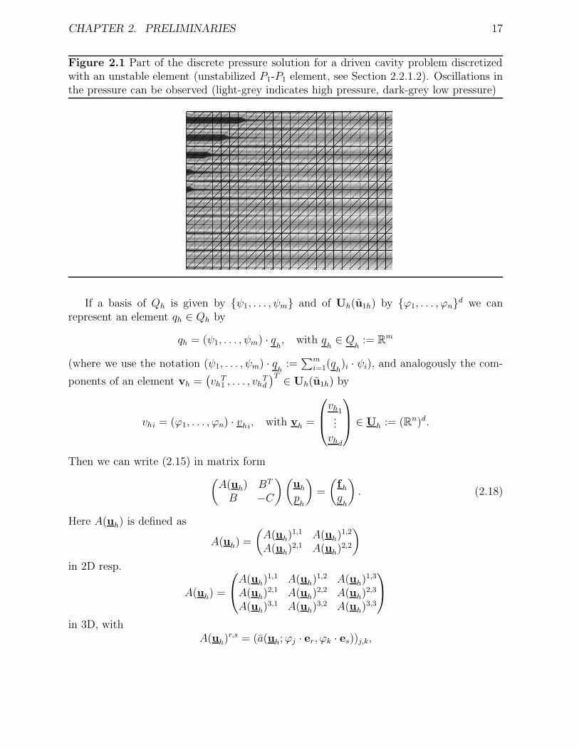
Remark 2.5. In literature (e.g. [GR86], [BF91], or [Bra97]) one can find prominent exam-ples of what can go wrong with elements not fulfilling the inf-sup condition (‘checkerboard’-instabilities, spurious pressure modes, etc.). The discrete solution may contain unphysicaloscillations and may for h → 0 not converge to the solution of the continuous problem,what is illustrated in Figure 2.1
CHAPTER 2. PRELIMINARIES 17
Figure 2.1 Part of the discrete pressure solution for a driven cavity problem discretizedwith an unstable element (unstabilized P1-P1 element, see Section 2.2.1.2). Oscillations inthe pressure can be observed (light-grey indicates high pressure, dark-grey low pressure)
If a basis of Qh is given by ψ1, . . . , ψm and of Uh(u1h) by ϕ1, . . . , ϕnd we canrepresent an element qh ∈ Qh by
qh = (ψ1, . . . , ψm) · qh, with q
h∈ Q
h:= Rm
(where we use the notation (ψ1, . . . , ψm) · qh
:=∑m
i=1(qh)i · ψi), and analogously the com-
ponents of an element vh =(vhT1 , . . . , vh
Td
)T ∈ Uh(u1h) by
vhi = (ϕ1, . . . , ϕn) · vhi, with vh =
vh1...vhd
∈ Uh := (Rn)d.
Then we can write (2.15) in matrix form(A(uh) BT
B −C
)(uhph
)=
(fhgh
). (2.18)
Here A(uh) is defined as
A(uh) =
(A(uh)
1,1 A(uh)1,2
A(uh)2,1 A(uh)
2,2
)
in 2D resp.
A(uh) =
A(uh)
1,1 A(uh)1,2 A(uh)
1,3
A(uh)2,1 A(uh)
2,2 A(uh)2,3
A(uh)3,1 A(uh)
3,2 A(uh)3,3
in 3D, withA(uh)
r,s = (a(uh;ϕj · er, ϕk · es))j,k,
CHAPTER 2. PRELIMINARIES 18
where er is the r-th unity vector in Rd. For a(.; ., .) as defined above we get
A(uh)r,s ≡ 0 if r 6= s.
Analogously B is defined by the relation
B =(B1 B2
)
in 2D resp.B =
(B1 B2 B3
)
in 3D, withBr = b(ϕj · er, ψk))j,k,
and C byC = (c(ψj, ψk))j,k.
In the same manner we define the mass matrix
M = ((ϕj, ϕk)0)j,k,
the pressure mass matrixMp = ((ψj, ψk)0)j,k,
and the LaplacianAD = (aD(ϕj, ϕk))j,k,
which we will need later in this thesis.We denote the FE-isomorphisms between the discrete spaces and the spaces of coeffi-
cient vectors by φU : (Rn)d → Uh(u1h) and φQ : Rm → Qh. The underline notation is usedto indicate their inverses, i.e.
φUvh = vh, φUvh = vh, (2.19)
φQqh = qh, φQqh = qh. (2.20)
If it is clear from the context we omit the underlines and φ’s and identify vh ∈ Uh(u1h)and the associated vh ∈ (Rn)d and analogously qh and q
h.
2.2.1 Examples of Mixed Elements
We present some popular choices of finite element pairs Uh × Qh, in particular those wewill use later for the construction of algebraic multigrid methods and in the numericalexamples, all of them based on triangular resp. tetrahedral elements. Thus, we assumethat some partitioning of G into triangles resp. tetrahedra G =
⋃i τi is given, we denote
the diameter of an element τi by hτi , we assume that we can identify some typical diameterh (the discretization parameter) with
αh ≤ hτi ≤ αh for all i,
where α and α are some positive constants, and we denote the set of elements by Th =τ1, τ2, . . .. On each element τi we define the space Pk(τi) of polynomials of degree lessthan or equal k.
CHAPTER 2. PRELIMINARIES 19
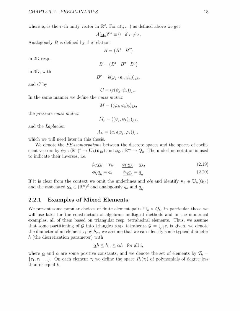
Figure 2.2 Some mixed finite elements for triangles (first row) and tetrahedra (secondrow). The circles/spheres indicate degrees of freedom for velocity-components, the boxesfor pressure.
(a) Taylor-Hood (b) P1-P1 (c) Crouzeix-Raviart
2.2.1.1 (Modified) Taylor-Hood Element
For the Taylor-Hood element, or P2-P1 element, we specify
Uh = vh ∈ U : vh|τi ∈ P2(τi)d for all elements τi,
Qh = qh ∈ Q : qh|τi ∈ P1(τi) for all elements τi.(2.21)
An element (vh, qh) in Uh × Qh is uniquely determined by specifying the values of the dcomponents of vh on the nodes and on the midpoints of edges of the elements and thevalues of qh on the nodes of the elements as illustrated in Figure 2.2(a).
The so called modified Taylor-Hood element, or P1isoP2-P1, is a mixed element withthe same degrees of freedom as the classical Taylor-Hood element, which is obtained thefollowing way. We take Qh as in (2.21), and then refine the mesh as indicated in the 2D-part of Figure 2.2(a): we divide each triangle into four subtriangles, each tetrahedron intoeight subtetrahedra, and get the finer partitioning G =
⋃i τi. There we define the velocity
spaceUh = vh ∈ U : vh|τi ∈ P1(τi)
d for all (sub-) elements τi.Both the classical Taylor-Hood element and the modified one fulfill the discrete inf-
sup condition as shown in [BF91]. Thus, their precision can be directly estimated using(2.17) and the well known approximation results for P1 resp. P2 elements. For the classical
CHAPTER 2. PRELIMINARIES 20
element we get
‖u− uh‖1 + ‖p− ph‖0 ≤ Cht(|u|t+1 + |p|t), for t = 1 or t = 2,
if (u, p) ∈ H t+1(G)d × H t(G). For the modified element, only the estimate with t = 1remains true.
2.2.1.2 Stabilized P1-P1 Element
If we use piecewise linear basis functions for both pressure and velocity components (Figure2.2(b)) we obtain an element which is very easy to implement in a concrete computerprogram but unfortunately does not fulfill the discrete inf-sup condition. As mentionedin Remark 2.5, numerical solutions computed using this element often contain unphysicalpressure modes which prevent convergence against the solution of the continuous problem.A possible way out is the introduction of the following stabilizing c(., .) term in (2.15)
c(p, q) = αS∑
i
h2τi
(∇p,∇q)0,τi, (2.22)
and a right hand side term to preserve consistency
〈G, q〉 = −αS∑
i
h2τi
(f ,∇q)0,τi , (2.23)
where αS is a positive parameter (intensive discussion on the correct choice of this param-eter and the local mesh size hτi can be found for example in [Bec95] or [FM93]). We willrefer to this stabilized element as P1-P1-stab.
Remark 2.6. Another possibility of stabilizing the P1-P1 element leads to the so called MINI-element. Here the velocity space is extended by bubble functions, i.e. uh is an element ofUh with
Uh := v ∈ U : v|τi = w|τi + bτi ατi with w ∈ Uh and ατi ∈ Rd,where bτi(x) =
∏j λj(x), and λj(x) are the barycentric coordinates of x with respect to τi.
It is possible to locally eliminate the bubble-variables, which leads to a similar problem as(2.15),(2.22),(2.23), with slightly more information on the choice of αS, e.g. that it shouldbe of order O(1/ν).
Although this element does not fulfill the inf-sup condition, the following result holds(without proof)
Theorem 2.7. [FS91, theorem 3.1] Suppose that the solution of the continuous Stokes prob-lem satisfies u ∈ H2(G)d and p ∈ H2(G). Then for αS > 0 the problem (2.15),(2.22),(2.23)has a unique solution, satisfying
‖u− uh‖1 + ‖p− ph‖0 ≤ C(h|u|2 + h2|p|2). (2.24)
CHAPTER 2. PRELIMINARIES 21
2.2.1.3 Crouzeix-Raviart Element
Here we drop the requirement that the finite dimensional spaces have to be subsets ofthe continuous spaces, insofar as the functions in Uh will not be continuous. We usenonconforming P1 velocity components (P nc
1 for short), i.e. we define
Uh = vh : vh|τi ∈ P1(τi)d for all elements τi,
vh is continuous at the midpoints of all element-edges/faces (in 2D/3D),
vh(bj) = 0 for all midpoints of boundary edges/faces bj on Γ1h.(2.25)
andQh = qh ∈ Q : qh|τi ∈ P0(τi) for all elements τi. (2.26)
The elements in Uh × Qh are determined by their velocity values at the edge-/face-centers and pressure values at the element centers (see 2.2(c)).
Detailed analysis for this mixed element can be found in [CR73], for example theconvergence result
‖u− uh‖1 ≤ Ch(|u|2 + |p|1)
for (u, p) ∈ H2(G)d ×H1(G).A nice property of the Crouzeix-Raviart element is the element-wise mass conservation,
which is enforced by the piecewise constant pressure discretization.Note that the term “Crouzeix-Raviart element”, which we use for P nc
1 -P0, is oftenassociated to different elements, for example (scalar) P nc
1 or the divergence-free P nc1 ele-
ment (where a divergence-free basis for the velocities is constructed, and the pressure cantherefore be eliminated from the equations).
In the following we will often drop the h subscripts if it is obvious from the context.
2.2.2 Multi-Element Meshes
All the elements presented above are based on a mesh consisting of triangles resp. tetra-hedra. We want to mention that they have counterparts for quadrilateral resp. hexahedralmeshes, but we will not go into detail and refer to literature, especially [BF91] and [Tur99].
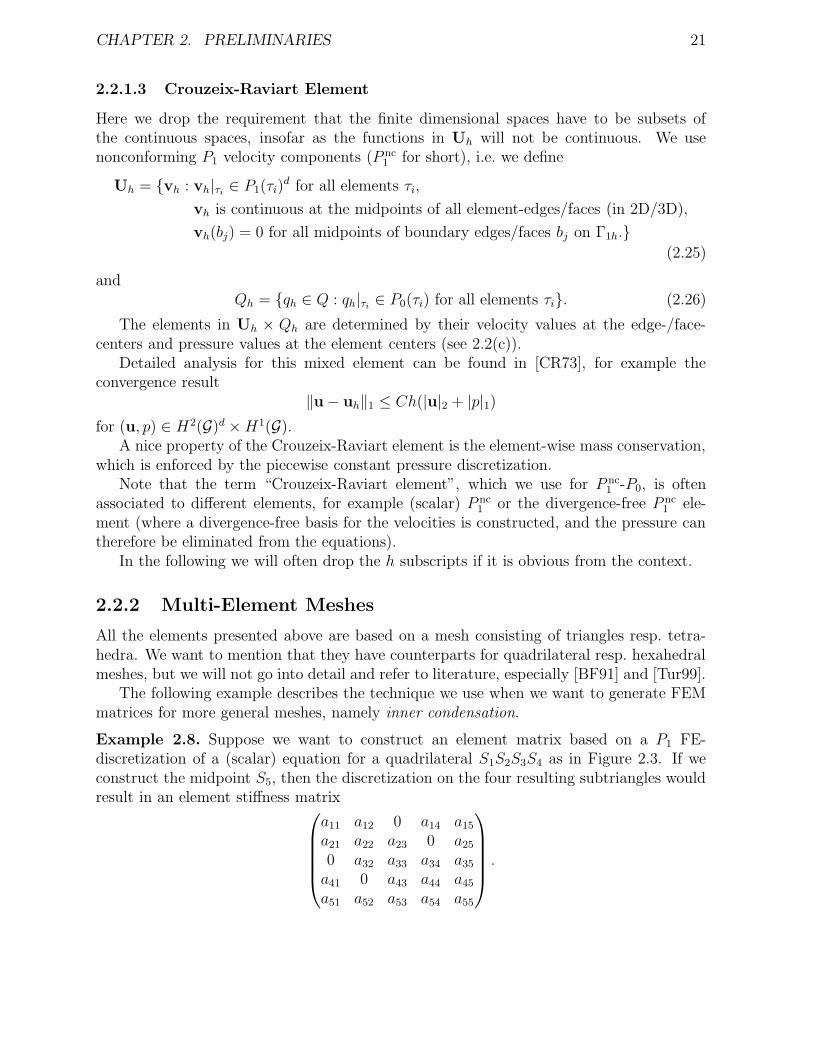
The following example describes the technique we use when we want to generate FEMmatrices for more general meshes, namely inner condensation.
Example 2.8. Suppose we want to construct an element matrix based on a P1 FE-discretization of a (scalar) equation for a quadrilateral S1S2S3S4 as in Figure 2.3. If weconstruct the midpoint S5, then the discretization on the four resulting subtriangles wouldresult in an element stiffness matrix
a11 a12 0 a14 a15
a21 a22 a23 0 a25
0 a32 a33 a34 a35
a41 0 a43 a44 a45
a51 a52 a53 a54 a55
.
CHAPTER 2. PRELIMINARIES 22
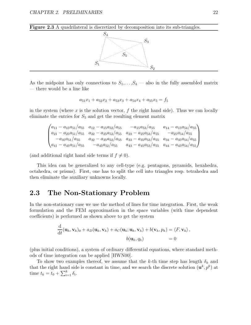
Figure 2.3 A quadrilateral is discretized by decomposition into its sub-triangles.
PSfrag replacements
S1S2
S3
S4
S5
As the midpoint has only connections to S1,. . . ,S4 — also in the fully assembled matrix— there would be a line like
a51x1 + a52x2 + a53x3 + a54x4 + a55x5 = f5
in the system (where x is the solution vector, f the right hand side). Thus we can locallyeliminate the entries for S5 and get the resulting element matrix
a11 − a15a51/a55 a12 − a15a52/a55 −a15a53/a55 a14 − a15a54/a55
a21 − a25a51/a55 a22 − a25a52/a55 a23 − a25a53/a55 −a25a54/a55
−a35a51/a55 a32 − a35a52/a55 a33 − a35a53/a55 a34 − a35a54/a55
a41 − a45a51/a55 −a45a52/a55 a43 − a45a53/a55 a44 − a45a54/a55
(and additional right hand side terms if f 6= 0).
This idea can be generalized to any cell-type (e.g. pentagons, pyramids, hexahedra,octahedra, or prisms). First, one has to split the cell into triangles resp. tetrahedra andthen eliminate the auxiliary unknowns locally.
2.3 The Non-Stationary Problem
In the non-stationary case we use the method of lines for time integration. First, the weakformulation and the FEM approximation in the space variables (with time dependentcoefficients) is performed as shown above to get the system
d
dt(uh,vh)0 + aD(uh,vh) + aC(uh; uh,vh) + b(vh, ph) = 〈F,vh〉 ,
b(uh, qh) = 0
(plus initial conditions), a system of ordinary differential equations, where standard meth-ods of time integration can be applied [HWN00].
To show two examples thereof, we assume that the k-th time step has length δk andthat the right hand side is constant in time, and we search the discrete solution (uk, pk) attime tk = t0 +
∑ki=1 δi.
CHAPTER 2. PRELIMINARIES 23
The first example is the one-step-θ scheme, which takes the matrix form
[1
δkM + θA(uk)
]uk +BTpk =
[1
δkM + (θ − 1)A(uk−1)
]uk−1 + f ,
Buk − Cpk = g.
The parameter θ can be chosen in [0, 1], θ = 0 gives the explicit Euler scheme, θ = 1 theimplicit Euler scheme, and θ = 0.5 the Crank-Nicolson scheme scheme.
As second example we present the fractional-step-θ-scheme, where each time step isdivided into three substeps (tk−1 → tk−1+θ → tk−θ → tk):
1.)
[1
δkθM + αA(uk−1+θ)
]uk−1+θ+BTpk−1+θ =
[1
δkθM − βA(uk−1)
]uk−1 + f ,
Buk−1+θ −Cpk−1+θ = g,
2.)
[1
δkθ′M + βA(uk−θ)
]uk−θ +BTpk−θ =
[1
δkθ′M − αA(uk−1+θ)
]uk−1+θ + f ,
Buk−θ −Cpk−θ = g,
3.)
[1
δkθM + αA(uk)
]uk +BTpk =
[1
δkθM − βA(uk−θ)
]uk−θ + f ,
Buk −Cpk = g,
with θ = 1 −√
22
, θ′ = 1 − 2θ, α ∈ ( 12, 1] and β = 1 − α (where the choice α = 1−2θ
1−θ isconvenient for implementation, because then αθ = βθ′).
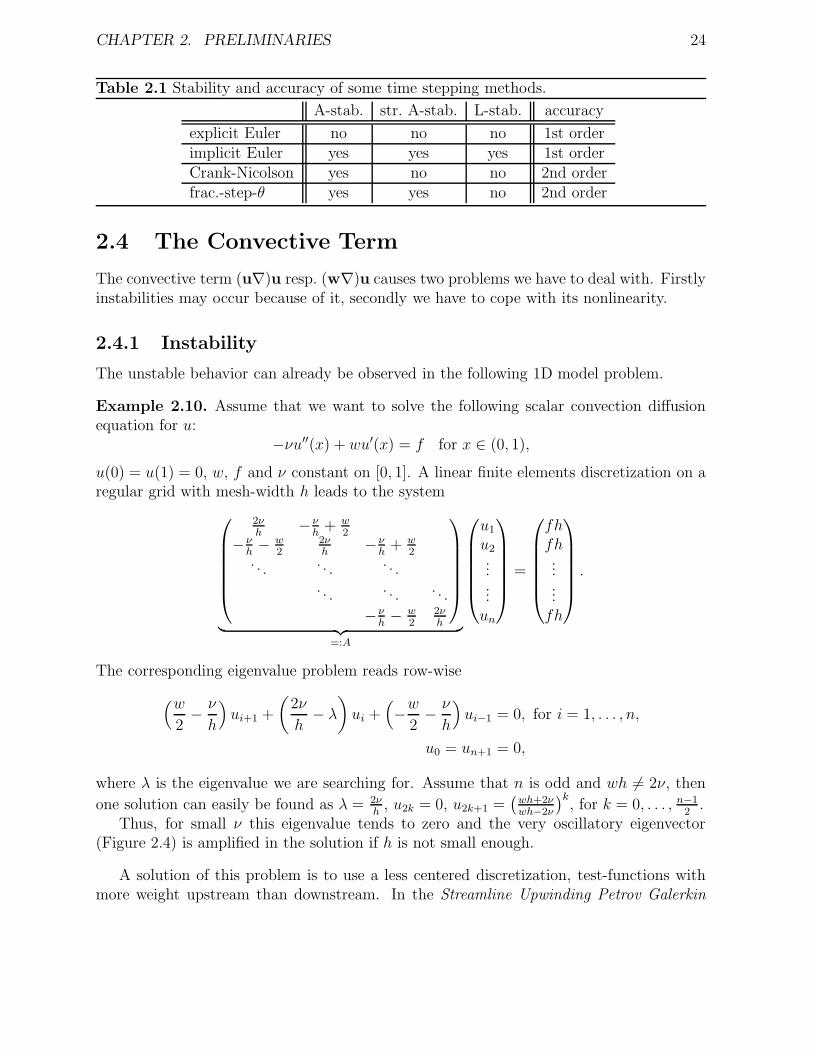
In Table 2.1 we list convergence and stability properties of this schemes without goinginto the details and without giving any motivation for this properties (what can be foundin [Ran00] or [HW02]). The terms used are described in the following definition.
Definition 2.9. Assume that the discrete solution (with constant time step length) of thetest-problem
y′(t) = λy(t), y(0) = y0,
with λ ∈ C has the formyk = R(δλ)yk−1,
where R(z) is called the stability function. A scheme is said to be
• A-stable if |R(z)| ≤ 1 for all z ∈ C− := z ∈ C : Re z ≤ 0,
• strongly A-stable if it is A-stable and limz→∞R(z) < 1, and
• L-stable if it is A-stable and limz→∞R(z) = 0.
CHAPTER 2. PRELIMINARIES 24
Table 2.1 Stability and accuracy of some time stepping methods.
A-stab. str. A-stab. L-stab. accuracy
explicit Euler no no no 1st orderimplicit Euler yes yes yes 1st orderCrank-Nicolson yes no no 2nd orderfrac.-step-θ yes yes no 2nd order
2.4 The Convective Term
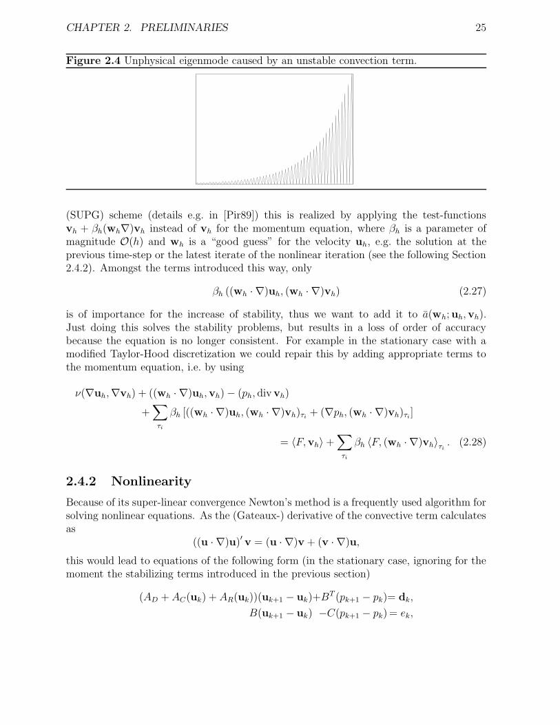
The convective term (u∇)u resp. (w∇)u causes two problems we have to deal with. Firstlyinstabilities may occur because of it, secondly we have to cope with its nonlinearity.
2.4.1 Instability
The unstable behavior can already be observed in the following 1D model problem.
Example 2.10. Assume that we want to solve the following scalar convection diffusionequation for u:
−νu′′(x) + wu′(x) = f for x ∈ (0, 1),
u(0) = u(1) = 0, w, f and ν constant on [0, 1]. A linear finite elements discretization on aregular grid with mesh-width h leads to the system
2νh
− νh
+ w2
− νh− w
22νh
− νh
+ w2
. . .. . .
. . .. . .
. . .. . .
− νh− w
22νh
︸ ︷︷ ︸=:A
u1
u2......un
=
fhfh......fh
.
The corresponding eigenvalue problem reads row-wise
(w2− ν
h
)ui+1 +
(2ν
h− λ)ui +
(−w
2− ν
h
)ui−1 = 0, for i = 1, . . . , n,
u0 = un+1 = 0,
where λ is the eigenvalue we are searching for. Assume that n is odd and wh 6= 2ν, then
one solution can easily be found as λ = 2νh
, u2k = 0, u2k+1 =(wh+2νwh−2ν
)k, for k = 0, . . . , n−1
2.
Thus, for small ν this eigenvalue tends to zero and the very oscillatory eigenvector(Figure 2.4) is amplified in the solution if h is not small enough.
A solution of this problem is to use a less centered discretization, test-functions withmore weight upstream than downstream. In the Streamline Upwinding Petrov Galerkin
CHAPTER 2. PRELIMINARIES 25
Figure 2.4 Unphysical eigenmode caused by an unstable convection term.
(SUPG) scheme (details e.g. in [Pir89]) this is realized by applying the test-functionsvh + βh(wh∇)vh instead of vh for the momentum equation, where βh is a parameter ofmagnitude O(h) and wh is a “good guess” for the velocity uh, e.g. the solution at theprevious time-step or the latest iterate of the nonlinear iteration (see the following Section2.4.2). Amongst the terms introduced this way, only
βh ((wh · ∇)uh, (wh · ∇)vh) (2.27)
is of importance for the increase of stability, thus we want to add it to a(wh; uh,vh).Just doing this solves the stability problems, but results in a loss of order of accuracybecause the equation is no longer consistent. For example in the stationary case with amodified Taylor-Hood discretization we could repair this by adding appropriate terms tothe momentum equation, i.e. by using
ν(∇uh,∇vh) + ((wh · ∇)uh,vh)− (ph, div vh)
+∑
τi
βh [((wh · ∇)uh, (wh · ∇)vh)τi + (∇ph, (wh · ∇)vh)τi]
= 〈F,vh〉+∑
τi
βh 〈F, (wh · ∇)vh〉τi . (2.28)
2.4.2 Nonlinearity
Because of its super-linear convergence Newton’s method is a frequently used algorithm forsolving nonlinear equations. As the (Gateaux-) derivative of the convective term calculatesas
((u · ∇)u)′ v = (u · ∇)v + (v · ∇)u,
this would lead to equations of the following form (in the stationary case, ignoring for themoment the stabilizing terms introduced in the previous section)
(AD + AC(uk) + AR(uk))(uk+1 − uk)+BT (pk+1 − pk)= dk,
B(uk+1 − uk) −C(pk+1 − pk) = ek,
CHAPTER 2. PRELIMINARIES 26
where AR(w)u is the discretization of (u·∇)w, (uk, pk) are the Newton iterates and (dk, ek)are some defect right hand sides.
Unfortunately the zero order reaction term AR poses two problems. Firstly it addsblock-off-diagonal entries to matrix A which increase its computational complexity, sec-ondly it has an uncontrollable effect on the diagonal of A and could cause divergence. Thusit is common practice to drop this term. This leads to the fixed point method, where ineach iteration step the Oseen equations have to be solved.
A third possibility would be to use (few steps of) an Oseen-preconditioned Richardson-iteration for the linear problem in each Newton-step, which avoids the reaction term in thesystem matrix but puts it to the right hand side.
In the case of strongly dominant convection and stationary equations, the nonlineariteration is often hard to control. As this is less the case when solving the instationaryproblem, we introduce a pseudo time term, i.e. we obtain an iterative process where uk+1
and pk+1 satisfy (A(uk) + αM BT
B −C
)(uk+1
pk+1
)=
(f + αMuk
g
),
where M is the mass matrix or (as we are not interested in the correct reconstruction of anon-stationary process) a lumped mass matrix and α a (small) parameter.
Besides the stabilization of the nonlinear process, this method has the nice property ofincreasing the symmetry of the linear systems.
Summing up, the resulting linear saddle point system which has to be solved (once orfor every nonlinear iteration step and/or for every time step) has the general form (wherewe denote the block matrix with K, the solution block vector with x, and the right handside block vector with b)
Kx :=
(A(w) BT
B −C
)(up
)=
(fg
)=: b, (2.29)
withA(w) = c1M + AD + c2AC(w) + c3AS(w) + c4AR(w), (2.30)
with mass matrix M , symmetric positive definite Laplacian AD, non-symmetric convectionAC and reaction AR, symmetric positive semi-definite convection stabilization AS and con-stants c1,. . . ,c4 which may be zero, and symmetric positive semi-definite (or zero) elementstabilization C.
Because of (2.28) it may occur that we have no symmetry in the off-diagonal blocks,i.e. (
A(w) BT1
B2 −C
),
with B1 6= B2. We will not deal with this situation separately in the remaining of thisthesis, but assume the form (2.29). Note that the case B1 6= B2 would not cause anyadditional problems, because then a dominating non-symmetry is already found in A(w).Therefore we have to deal with a (substantial) non-symmetric system matrix anyway.
CHAPTER 2. PRELIMINARIES 27
2.5 Iterative Solvers
In this section we give a brief overview over (non-multigrid) iterative solvers which areapplicable to the saddle point system (2.29). Of course, there is a great variety of possiblemethods, we have only chosen some prominent examples.
2.5.1 Krylov Space Methods
A first possible family of solvers are those (preconditioned) Krylov space methods whichare capable of solving indefinite and (in the non-Stokes case) non-symmetric problems.Examples thereof are GMRES and the BiCGstab. An overview of more Krylov spacemethods can be found for example in [Vos93] or [Meu99].
2.5.1.1 GMRES
The generalized minimal residual method (GMRES), introduced in [SS86], is a generaliza-tion of the MINRES method to the non-symmetric case. The idea is to solve in the k-thiteration step the least squares problem: Find y ∈ Rk such that
‖b−K(x0 +Qky)‖`2 → min,
where the column vectors of Qk build an orthonormal (w.r.t. the `2-scalar product) basisof the k-th Krylov space
Kk(b, K) = spanb, Kb, . . . , Kk−1b.
Thus, it could be seen as an exact method, which stops at the solution after finitely manysteps, but which uses an increasing amount of memory in each step. Therefore in practicewe use the GMRES(m) method, i.e. GMRES restarted periodically after m steps.
Algorithm 2.11. Preconditioned GMRES(m). Iterative Solution of Kx = b, withpreconditioner K.
Choose starting solution x0;
q1 = K−1(b−Kx0);z1 = ‖q1‖;q1 = (1/z1) · q1;repeat
beginfor k = 1 to m do
begin
qk+1 = K−1Kqk;for i = 1 to k do
beginhik = qi · qk+1; qk+1 = qk+1 − hikqi;
CHAPTER 2. PRELIMINARIES 28
endhk+1,k = ‖qk+1‖; qk+1 = qk+1/hk+1,k;
endfor k = 1 to m do
begin
cc =√h2kk + h2
k+1,k;
c = hkk/cc; s = hk+1,k/cc; hkk = cc;for i = k + 1 to m do(
hk,ihk+1,i
)=
(c ss −c
)(hk,ihk+1,i
);
(zkzk+1
)=
(c ss −c
)(zk0
);
endym = zm/hmm;for i = m down-to 1 do
yi =(zi −
∑mj=i+1 hijyj
)/hii;
xm = x0 +∑m
i=1 yiqi;
rm = K−1(b−Kxm);x0 = xm; r0 = rm;z1 = ‖r0‖; q1 = (1/z1) · r0;
enduntil |z1| < tolerance
2.5.1.2 BiCGstab
The stabilized bi-conjugate gradient method (BiCGstab) was introduced in [VdV92] (withslight modifications in [SVdV94]). It is not optimal in each step, i.e. it solves the min-imization problem only approximately, but as it uses a short range recurrence for theconstruction of the orthonormal basis of the Krylov space, it consumes considerably lesscomputer memory as GMRES.
Algorithm 2.12. BiCGstab. Iterative Solution of Kx = b, with preconditioner K.
Choose starting solution x0;
r0 = K−1(b−Kx0);Choose arbitrary r0, such that r0 · r0 6= 0, e.g. r0 = r0;ρ0 = α = ω0 = 1;v0 = p0 = 0;i← 1;repeat
beginρi = r0 · ri−1; β = (ρi/ρi−1)(α/ωi−1);pi = ri−1 + β(pi−1 − ωi−1vi−1);
CHAPTER 2. PRELIMINARIES 29
y = Kpi; vi = K−1y;α = ρi/(r0 · vi);s = ri−1 − αvi;
y = Ks; t = K−1y;ωi = (t · s)/(t · t);xi = xi−1 + αpi + ωis;if xi is accurate enough then quit;
ri = K−1(b−Kxi);i← i+ 1;
end
2.5.2 SIMPLE
If linear solvers for scalar elliptic equations are available, a very popular method is SIM-PLE (Semi-Implicit Method for Pressure-Linked Equations), developed by Patankar andSpalding [PS72, Pat80], which iteratively decouples the system to equations for pressureand for velocity (even for velocity-components in the Oseen or in the Stokes case as thenA is block-diagonal).
We start with the factorization
K =
(A 0B S
)(I A−1BT
0 −I
), (2.31)
with the Schur complement S = C+BA−1BT , and then introduce preconditioners A for A
in the first factor,ˆA for A in the second factor and S for S. Using this in a preconditioned
Richardson method leads to the scheme
A(uk+1 − uk) = f − Auk − BTpk, (2.32a)
S(pk+1 − pk) = Buk+1 − Cpk − g, (2.32b)
ˆA(uk+1 − uk+1) = −BT (pk+1 − pk), (2.32c)
where uk+1 is some auxiliary vector. Now in (2.32a) Auk is replaced by Auk, leading to
Auk+1 = f − BTpk.
In the classical SIMPLE algorithm S is a preconditioner for the modified Schur complement
C +BˆA−1BT ,
ˆA is the diagonal of A, denoted by D, and the pressure update is damped.
This leads to the following algorithm.
CHAPTER 2. PRELIMINARIES 30
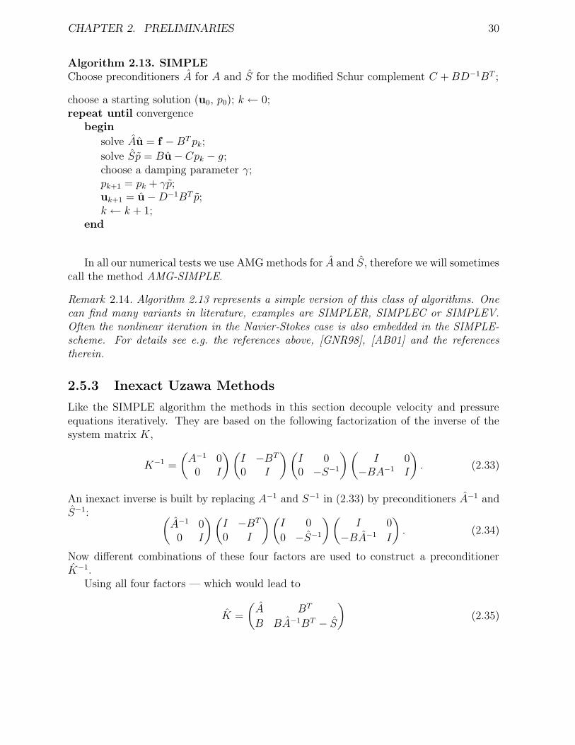
Algorithm 2.13. SIMPLEChoose preconditioners A for A and S for the modified Schur complement C +BD−1BT ;
choose a starting solution (u0, p0); k ← 0;repeat until convergence
begin
solve Au = f −BT pk;
solve Sp = Bu− Cpk − g;choose a damping parameter γ;pk+1 = pk + γp;uk+1 = u−D−1BT p;k ← k + 1;
end
In all our numerical tests we use AMG methods for A and S, therefore we will sometimescall the method AMG-SIMPLE.
Remark 2.14. Algorithm 2.13 represents a simple version of this class of algorithms. Onecan find many variants in literature, examples are SIMPLER, SIMPLEC or SIMPLEV.Often the nonlinear iteration in the Navier-Stokes case is also embedded in the SIMPLE-scheme. For details see e.g. the references above, [GNR98], [AB01] and the referencestherein.
2.5.3 Inexact Uzawa Methods
Like the SIMPLE algorithm the methods in this section decouple velocity and pressureequations iteratively. They are based on the following factorization of the inverse of thesystem matrix K,
K−1 =
(A−1 0
0 I
)(I −BT
0 I
)(I 00 −S−1
)(I 0
−BA−1 I
). (2.33)
An inexact inverse is built by replacing A−1 and S−1 in (2.33) by preconditioners A−1 andS−1: (
A−1 00 I
)(I −BT
0 I
)(I 0
0 −S−1
)(I 0
−BA−1 I
). (2.34)
Now different combinations of these four factors are used to construct a preconditionerK−1.
Using all four factors — which would lead to
K =
(A BT
B BA−1BT − S
)(2.35)
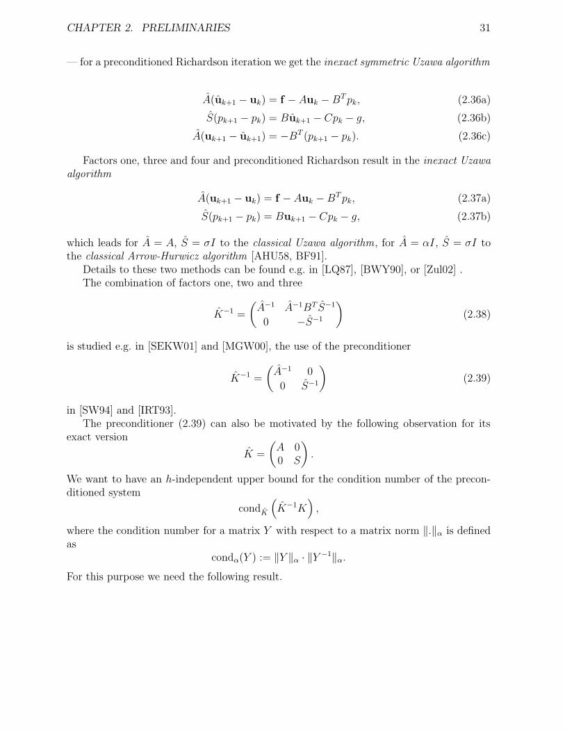
CHAPTER 2. PRELIMINARIES 31
— for a preconditioned Richardson iteration we get the inexact symmetric Uzawa algorithm
A(uk+1 − uk) = f − Auk − BTpk, (2.36a)
S(pk+1 − pk) = Buk+1 − Cpk − g, (2.36b)
A(uk+1 − uk+1) = −BT (pk+1 − pk). (2.36c)
Factors one, three and four and preconditioned Richardson result in the inexact Uzawaalgorithm
A(uk+1 − uk) = f − Auk − BTpk, (2.37a)
S(pk+1 − pk) = Buk+1 − Cpk − g, (2.37b)
which leads for A = A, S = σI to the classical Uzawa algorithm, for A = αI, S = σI tothe classical Arrow-Hurwicz algorithm [AHU58, BF91].
Details to these two methods can be found e.g. in [LQ87], [BWY90], or [Zul02] .The combination of factors one, two and three
K−1 =
(A−1 A−1BT S−1
0 −S−1
)(2.38)
is studied e.g. in [SEKW01] and [MGW00], the use of the preconditioner
K−1 =
(A−1 0
0 S−1
)(2.39)
in [SW94] and [IRT93].The preconditioner (2.39) can also be motivated by the following observation for its
exact version
K =
(A 00 S
).
We want to have an h-independent upper bound for the condition number of the precon-ditioned system
condK
(K−1K
),
where the condition number for a matrix Y with respect to a matrix norm ‖.‖α is definedas
condα(Y ) := ‖Y ‖α · ‖Y −1‖α.For this purpose we need the following result.
CHAPTER 2. PRELIMINARIES 32
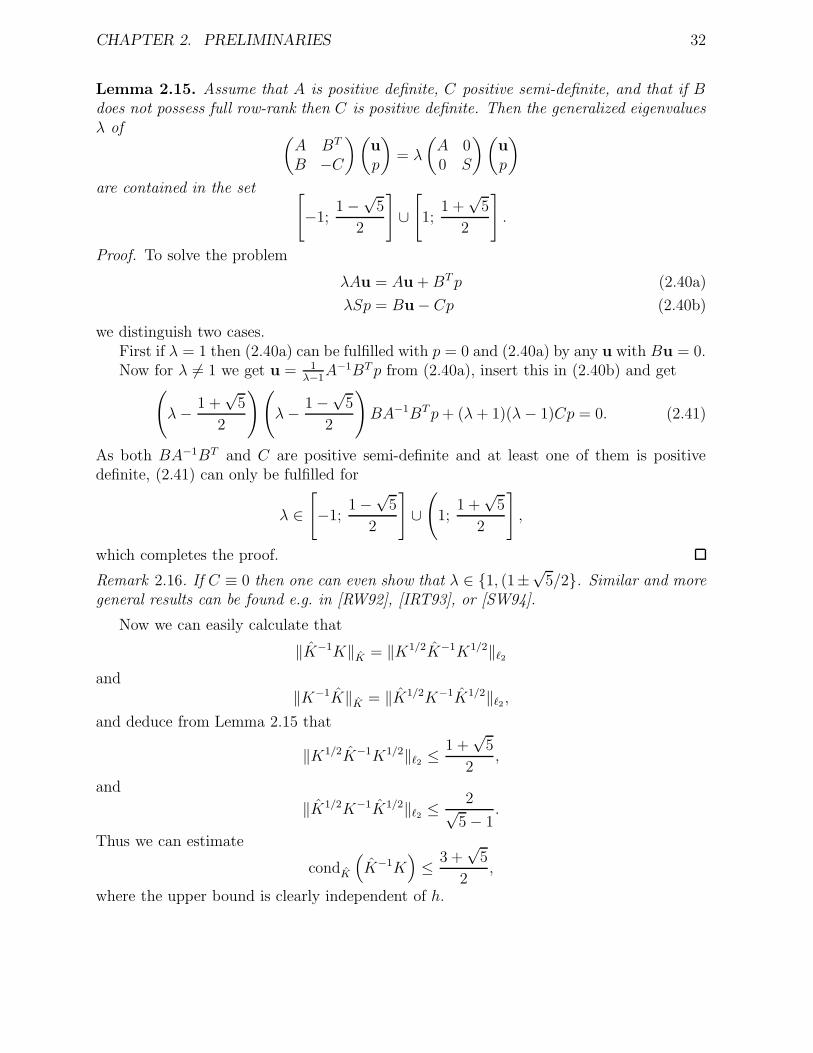
Lemma 2.15. Assume that A is positive definite, C positive semi-definite, and that if Bdoes not possess full row-rank then C is positive definite. Then the generalized eigenvaluesλ of (
A BT
B −C
)(up
)= λ
(A 00 S
)(up
)
are contained in the set [−1;
1−√
5
2
]∪[
1;1 +√
5
2
].
Proof. To solve the problem
λAu = Au +BT p (2.40a)
λSp = Bu− Cp (2.40b)
we distinguish two cases.First if λ = 1 then (2.40a) can be fulfilled with p = 0 and (2.40a) by any u with Bu = 0.Now for λ 6= 1 we get u = 1
λ−1A−1BT p from (2.40a), insert this in (2.40b) and get
(λ− 1 +
√5
2
)(λ− 1−
√5
2
)BA−1BTp+ (λ+ 1)(λ− 1)Cp = 0. (2.41)
As both BA−1BT and C are positive semi-definite and at least one of them is positivedefinite, (2.41) can only be fulfilled for
λ ∈[−1;
1−√
5
2
]∪(
1;1 +√
5
2
],
which completes the proof.
Remark 2.16. If C ≡ 0 then one can even show that λ ∈ 1, (1±√
5/2. Similar and moregeneral results can be found e.g. in [RW92], [IRT93], or [SW94].
Now we can easily calculate that
‖K−1K‖K = ‖K1/2K−1K1/2‖`2and
‖K−1K‖K = ‖K1/2K−1K1/2‖`2 ,and deduce from Lemma 2.15 that
‖K1/2K−1K1/2‖`2 ≤1 +√
5
2,
and
‖K1/2K−1K1/2‖`2 ≤2√
5− 1.
Thus we can estimate
condK
(K−1K
)≤ 3 +
√5
2,
where the upper bound is clearly independent of h.
CHAPTER 2. PRELIMINARIES 33
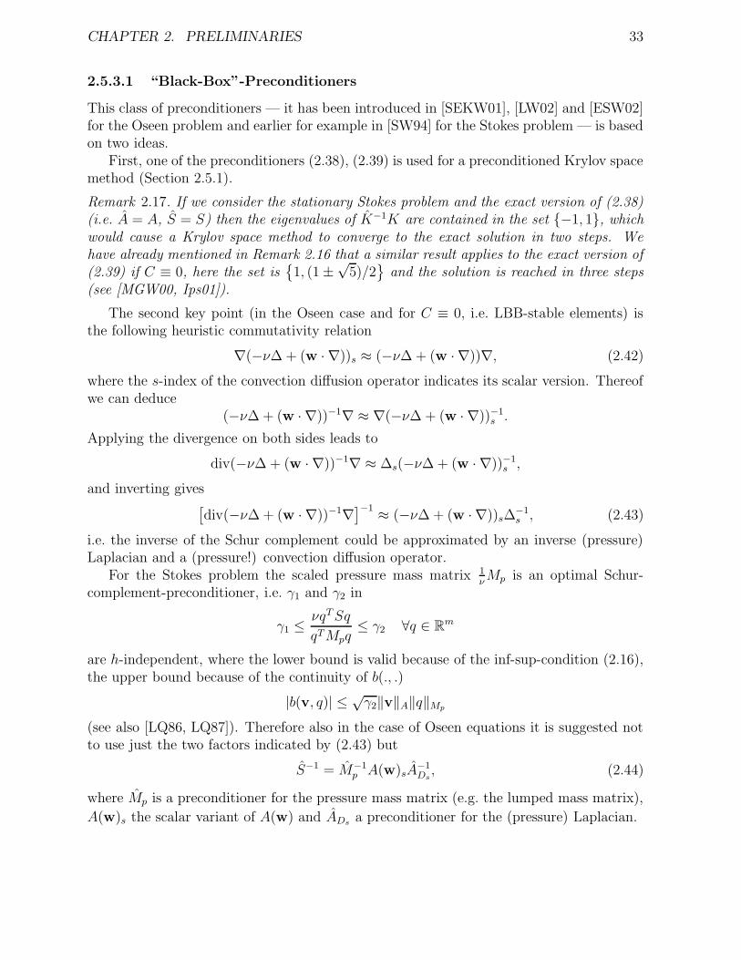
2.5.3.1 “Black-Box”-Preconditioners
This class of preconditioners — it has been introduced in [SEKW01], [LW02] and [ESW02]for the Oseen problem and earlier for example in [SW94] for the Stokes problem — is basedon two ideas.
First, one of the preconditioners (2.38), (2.39) is used for a preconditioned Krylov spacemethod (Section 2.5.1).
Remark 2.17. If we consider the stationary Stokes problem and the exact version of (2.38)(i.e. A = A, S = S) then the eigenvalues of K−1K are contained in the set −1, 1, whichwould cause a Krylov space method to converge to the exact solution in two steps. Wehave already mentioned in Remark 2.16 that a similar result applies to the exact version of(2.39) if C ≡ 0, here the set is
1, (1±
√5)/2
and the solution is reached in three steps
(see [MGW00, Ips01]).
The second key point (in the Oseen case and for C ≡ 0, i.e. LBB-stable elements) isthe following heuristic commutativity relation
∇(−ν∆ + (w · ∇))s ≈ (−ν∆ + (w · ∇))∇, (2.42)
where the s-index of the convection diffusion operator indicates its scalar version. Thereofwe can deduce
(−ν∆ + (w · ∇))−1∇ ≈ ∇(−ν∆ + (w · ∇))−1s .
Applying the divergence on both sides leads to
div(−ν∆ + (w · ∇))−1∇ ≈ ∆s(−ν∆ + (w · ∇))−1s ,
and inverting gives[div(−ν∆ + (w · ∇))−1∇
]−1 ≈ (−ν∆ + (w · ∇))s∆−1s , (2.43)
i.e. the inverse of the Schur complement could be approximated by an inverse (pressure)Laplacian and a (pressure!) convection diffusion operator.
For the Stokes problem the scaled pressure mass matrix 1νMp is an optimal Schur-
complement-preconditioner, i.e. γ1 and γ2 in
γ1 ≤νqTSq
qTMpq≤ γ2 ∀q ∈ Rm
are h-independent, where the lower bound is valid because of the inf-sup-condition (2.16),the upper bound because of the continuity of b(., .)
|b(v, q)| ≤ √γ2‖v‖A‖q‖Mp
(see also [LQ86, LQ87]). Therefore also in the case of Oseen equations it is suggested notto use just the two factors indicated by (2.43) but
S−1 = M−1p A(w)sA
−1Ds, (2.44)
where Mp is a preconditioner for the pressure mass matrix (e.g. the lumped mass matrix),
A(w)s the scalar variant of A(w) and ADs a preconditioner for the (pressure) Laplacian.
CHAPTER 2. PRELIMINARIES 34
Remark 2.18. Two possible problems of this preconditioner can arise of the assumption(2.42). First, the commutativity
∇[(w · ∇)] ≈ (w · ∇)∇,
is not fulfilled in general (except for some special situation, e.g. constant w), what posesproblems if this term dominates (for small ν’s).
Second, for non-constant ν (e.g. due to a k-ε turbulence model, c.f. [MP94] or [RW99])even the first part of (2.42) would be violated, as in this case
∇ν∆ 6= ν∆∇.
Chapter 3
Multigrid Methods
In the previous chapter we have introduced some iterative methods for the solution ofsaddle point systems, most of them having in common that (without preconditioning)they are not optimal, i.e. the number of arithmetical operations Q(ε) for a reduction of theresidual by a factor ε is considerably larger than O(n), where n is the number of unknownsof the system.
Multigrid methods, which will be the main topic in the remaining of this thesis, possessthis optimality-property Q(ε) = O(n) (at least geometric multigrid methods), thereforewe want to apply them as solvers (or preconditioners) for our system.
First we will describe a general algebraic multigrid (AMG) method, introduce thenotation and pinpoint some differences to geometric multigrid (GMG) methods. Then wewill give some concrete examples of methods for scalar elliptic equations.
3.1 A General Algebraic Multigrid Method
We want to construct a general AMG method for a set of linear equations
K1x = b1,
where K1 is a regular n1× n1 matrix. The index indicates the level, 1 is the finest level, Lwill be the coarsest. For AMG methods, which will be the main focus of this thesis, thisnumbering is natural, but note that it is the reverse of the natural numbering for GMGmethods.
The first step in this method is to create a full rank prolongation matrix P 12 based
on some coarsening (see later, Section 3.2.2), with P 12 : Rn2 → Rn1 and n2 < n1. For
this purpose (almost) only information from some auxiliary matrix H1 is used. Normallyone uses the information from the matrix K1, but the utilization of an auxiliary matrix(which is suggested for example in [Rei01]) enhances the flexibility of the method. In AMGmethods the size of the (negative) matrix entries is related to the strength of the couplingof two unknowns, thus different notions of ‘strength’ can be introduced for different choices
35
CHAPTER 3. MULTIGRID METHODS 36
of H1. One could use e.g.
(H1)i,j =
−1/‖ei,j‖ if i 6= j and vertex i and j are connected,∑k 6=i 1/‖ei,k‖ if i = j,
0 otherwise,
(3.1)
where ‖ei,j‖ is the length of the edge connecting the nodes i and j, to represent a virtualFE-mesh. For convection diffusion equations, this could be modified for regions withdominating convection, which causes a faster “transport of information”. More choicesseem conceivable, but will not be dealt with in this thesis.
We also need a restriction matrix R21 : Rn1 → Rn2 , for which we use R2
1 = (P 12 )T . Now
we can build the Galerkin projected matrix
K2 = R21K1P
12 ,
and the auxiliary matrix on this level
H2 = R21H1P
12 .
Repeating this step we end up with a set of prolongation matrices P ll+1, l = 1, . . . , L−1,
where P ll+1 : Rnl+1 → Rnl, n1 > n2 > . . . > nL, a set of restriction matrices Rl+1
l , and aset of coarse level matrices Kl and auxiliary matrices Hl with
Kl+1 = Rl+1l KlP
ll+1 (3.2)
andHl+1 = Rl+1
l HlPll+1.
Completing the AMG method we need on each level l = 1, . . . , L− 1 an iterative methodfor the problem Klxl = bl,
xj+1l = Sl(xjl , bl),
the smoothing operator.
CHAPTER 3. MULTIGRID METHODS 37
Algorithm 3.1. Basic multigrid iteration for the system Klxl = bl.Let mpre be the number of presmoothing steps, mpost of postsmoothing steps. Suppose wehave chosen a starting solution x0
l on level l.
for k ← 1 to mpre do xkl = Sl(xk−1l , bl); (presmoothing)
bl+1 ← Rl+1l (bl −Klx
mpre
l ); (restriction)if l + 1 = L
Compute the exact solution xL of KLxL = bL;else
beginApply Algorithm 3.1 (µ times) on
Kl+1xl+1 = bl+1
(with starting solution x0l+1 = 0)
and get xl+1;end
xmpre+1l ← x
mpre
l + P ll+1xl+1; (prolongation and correction)
for k ← 1 to mpost do xmpre+k+1l = Sl(xpre+k
l , bl); (postsmoothing)
return xl ← xmpre+mpost+1l ;
The part from (restriction) to (prolongation and correction) will be referred to as “coarsegrid correction”.
Repeated application of this algorithm until fulfillment of some convergence criterionyields a basic AMG method. For µ = 1 the iteration is called a ‘V-cycle’, for µ = 2 ‘W-cycle’. We use the abbreviations V-mpre-mpost resp. W-mpre-mpost for a V- resp. W-cyclewith mpre presmoothing and mpost postsmoothing steps.
Geometric Multigrid. The base for GMG methods is a hierarchical sequence of finerand finer meshes. Each level has an associated grid, thus P l
l+1 and Rl+1l can be constructed
using geometric information of two consecutive meshes, the auxiliary matrices Hl are notneeded.
The coarse system matrices need not be built using the Galerkin approach (3.2), directdiscretization of the differential operator on the specific mesh can be performed. For non-nested FE spaces (e.g. velocity components of the Crouzeix-Raviart element in Section2.2.1.3) these two approaches differ, the direct discretization seems to be more natural.
3.1.1 Basic Convergence Analysis
The common denominator and key point of all multigrid methods is the splitting of theerror components in two classes. One that can be reproduced on coarser levels/grids andtherefore can be reduced by the coarse grid correction and one that has to be reduced bythe smoother. For the geometric multigrid method the first group consists typically of lowfrequency parts the second of high frequency parts of the error. The ability to cope with
CHAPTER 3. MULTIGRID METHODS 38
the first group is called approximation property, with the second smoothing property. The(optimal) convergence of the multigrid method is the consequence of their combination.
The Geometric Multigrid Case. Two classical techniques of proofing the convergenceof geometric multigrid methods assure two-grid convergence (which can be shown to implyW-cycle convergence) by different splittings of the two-grid iteration operator (withoutpostsmoothing)
Ml+1l := (I − P i
l+1K−1l+1R
l+1l Kl)Sml ,
where m is the number of smoothing steps (i.e. m = mpre in Algorithm 3.1) and Sl the itera-tion matrix of the smoother (for a preconditioned Richardson iteration with preconditionerKl we have Sl = I − K−1
l Kl).The first technique, which was mainly developed by the Russian school [Bac66, Ast71,
Kor77, Lan82] is based on a sum splitting. Here the projections P low and P high (whichproject on the subspaces spanned by the low and high frequency eigenvectors of the systemmatrix) are introduced, and the identity, decomposed into I = P low ⊕ P high, is insertedinto Ml+1
l (left of Sml ) to get the estimate
‖Ml+1l ‖ ≤ ‖(I − P i
l+1K−1l+1R
l+1l Kl)P
low‖‖Sl‖m
+ ‖(I − P il+1K
−1l+1R
l+1l Kl)‖‖P highSml ‖.
Two-grid convergence is then proven by showing that the term ‖(I−P il+1K
−1l+1R
l+1l Kl)P
low‖is small (the approximation property) and that ‖P highSml ‖ is arbitrary small for sufficientlymany smoothing steps m (the smoothing property).
The other classical technique can be found in Hackbusch [Hac85]. Here a productsplitting is constructed after inserting the identity I = K−1
l Kl into Ml+1l (left of Sml ).
Then again two properties have to be shown. One is the approximation property whichhere reads as
‖K−1l − P l
l+1K−1l+1R
l+1l ‖`2 ≤ c/‖Kl‖`2 (3.3)
the other the smoothing property
‖KlSml ‖`2 ≤ η(m)‖Kl‖`2 (3.4)
where c is a positive constant and η(m) the so called smoothing rate (independent of levell) with
η(m)→ 0 for m→∞.They together imply the convergence of the two-grid method if m is large enough.
Remark 3.2. Instead of (3.3) and (3.4) the approximation and smoothing properties areoften formulated directly using the h-scaling induced by Kl, i.e.
‖K−1l − P l
l+1K−1l+1R
l+1l ‖ ≤ chδl
and‖KlSml ‖ ≤ η(m)h−δl ,
with appropriate δ and ‖.‖.
CHAPTER 3. MULTIGRID METHODS 39
The Algebraic Multigrid Case. Convergence analysis for algebraic multigrid meth-ods has been mostly restricted to the symmetric positive definite case up to now. For asymmetric positive definite system matrix Kl the smoothing property (according to Rugeand Stuben [RS86]) takes the form
‖Sle‖2Kl≤ ‖e‖2
Kl− c1‖Kle‖2
D−1l
for all e, (3.5)
with c1 > 0 independent of e and Dl the diagonal of Kl. This implies that the smootherhas to reduce an error e strongly if ‖Kle‖D−1
lis large (compared to ‖e‖Kl). If additionally
the approximation property
‖(I − P ll+1K
−1l+1R
l+1l Kl)e‖2
Kl≤ c2‖Kl(I − P l
l+1K−1l+1R
l+1l Kl)e‖2
D−1l
(3.6)
is fulfilled with c2 independent of e then
‖Sl(I − P il+1K
−1l+1R
l+1i Kl)e‖2
Kl≤‖(I − P i
l+1K−1l+1R
l+1l Kl)e‖2
Kl
− c1‖Kl(I − P ll+1K
−1l+1R
l+1l Kl)e‖D−1
l
≤ (1− c1
c2)‖(I − P l
l+1K−1l+1R
l+1l Kl)e‖2
Kl
≤ (1− c1
c2)‖e‖2
Kl,
i.e. the two-grid algorithm with one postsmoothing step converges.
3.2 Examples in the Scalar Elliptic Case
Assume for this section, that the system we want to solve results from a FE approximationof the scalar elliptic model problem: Find u : G → R such that
∆u(x) = b(x) for x ∈ G,u(x) = 0 for x ∈ ∂G,
which leads to the linear systemK1u = b1.
3.2.1 Geometric Multigrid
Basic point wise iterations like the ω-Jacobi or the Gauss-Seidel method can be used assmoothers in the case of our model problem.
For nested FE spaces X1 ⊃ X2 ⊃ . . . (again the index indicates the level) the construc-tion of the prolongation is straight-forward, it only has to reproduce identity.
CHAPTER 3. MULTIGRID METHODS 40
In the case of non-nested spaces different strategies are needed. For the example of P nc1
finite elements (e.g. the velocity components of the Crouzeix-Raviart element) one coulduse
(P ll+1uh
)e
=
uh(e) if e is a fine grid edge inside a coarse grid element,12
[uh|τ1(e) + uh|τ2(e)] if e = τ1 ∩ τ2 for two coarse grid elements τ1, τ2
(3.7)(c.f. [BV90] or [Bre93]).
3.2.2 Algebraic Multigrid
We assume now that the discretization of our model problem is nodal based, i.e. eachunknown is associated with a unique mesh node.
The smoother can again consist of ω-Jacobi or Gauss-Seidel iterations. For the con-struction of the coarse levels, i.e. the assembling of the prolongation matrices there arevarious possibilities, we will describe those which will be important later in this theses.
3.2.2.1 AMG Based on C/F-Splitting
The classical AMG methods use a splitting of the set of nodes into a set of coarse nodes(C) which will also be used on the coarse level, and a set of fine nodes (F) which ‘live’ onlyon the fine level, details can be found in [BMR84], [RS86] or [Stu01a].
Suppose that — after such a splitting has been chosen — the unknowns are sortedF-unknowns (living on F-nodes) first, then C-unknowns (living on C-nodes). This inducesa block structuring of the linear system
Klu =
(K lFF K l
FC
K lCF K l
CC
)(uFuC
)=
(bFbC
)= b
(and the same structuring for Hl and P ll+1). Now for the prolongation it is obviously a
good choice to leave the C-unknowns unchanged, i.e. to use
P ll+1 =
(P FC
I
)(3.8)
(omitting the level index l in P FC ), where again there are many variants for P F
C , some ofthem will be described in what follows. All of them have in common that each coarse nodeprolongates only to a very restricted set of fine nodes to prevent fill-in in the coarse levelmatrices and a resulting explosion of complexity.
One possibility is to do averaging on the F nodes, i.e. we could define
(P FC )j,k =
1mj
if k is a neighboring C node of a F node j,
0 otherwise,(3.9)
where mj is the number of neighboring C nodes of the F node j, and the neighbor-relationis induced by non-zero entries in the auxiliary matrix Hl.
CHAPTER 3. MULTIGRID METHODS 41
Remark 3.3. If the fine level mesh was constructed by a hierarchical refinement of a coarsemesh, the C and F nodes are chosen accordingly, and the underlying discretization is theP1 element, then this strategy reproduces the geometric multigrid method.
A more sophisticated prolongation can be found in [Stu01a]. Before presenting it weneed the concepts of M-matrices and of essentially positive type matrices.
Definition 3.4. A matrix H = (hij) is called M-matrix if
1. hii > 0 for all i,
2. hij ≤ 0 for all i 6= j,
3. H is regular, and H−1 ≥ 0 (where here ‘≥’ is meant component-wise).
(One can skip the first requirement because it is a consequence of 2. and 3., see e.g. [Hac93].)
Definition 3.5. A matrix H = (hij) is said to be of essentially positive type if it is positivedefinite and there exists a constant ω > 0 such that for all e,
∑
i,j
(−hij)(ei − ej)2 ≥ ω∑
i,j
(−h−ij)(ei − ej)2, (3.10)
with
h−ij =
hij if hij < 0,
0 otherwise
(and h+ij = hij − h−ij).
Remark 3.6. If H is a M-matrix than condition (3.10) is fulfilled with ω = 1. The classof essentially positive type matrices was introduced to capture “almost M”-matrices withsmall positive off-diagonal entries which can be ‘repaired’ (see [Bra86]).
Lemma 3.7. If a matrix H is of essentially positive type with ω as in (3.10) then for all e
2
ωeTDHe ≥ eTHe, (3.11)
where DH is the diagonal of H.
Proof. It is easy to check that
2
ωeTDHe ≥ eTHe− 1
2
∑
j
∑
k 6=jhjk
[(2
ω− 1
)e2j + 2ejek +
(2
ω− 1
)e2k
]
︸ ︷︷ ︸=:Λ
and that(
2
ω− 2
)(e2j + e2
k) ≤(
2
ω− 1
)e2j + 2ejek +
(2
ω− 1
)e2k ≤
2
ω(e2j + e2
k).
CHAPTER 3. MULTIGRID METHODS 42
Thus
Λ ≤ 2
ω
∑
j,kj 6=k
hjk(e2j + e2
k)− 2∑
j,kj 6=k
h−jk(e2j + e2
k). (3.12)
With e = (0, . . . , 0, 1, 0, . . . , 0)T , the i-th unit vector, we get from (3.10)
∑
jj 6=i
hij ≤ ω∑
jj 6=i
h−ij,
which together with (3.12) givesΛ ≤ 0
and therefore completes the proof.
From now on we will writeA ≥ B
for two matrices A and B if A − B is positive semi-definite (or A > B if it is positivedefinite), e.g. we can express (3.11) as 2
ωDH ≥ H.
We shortly sketch the construction of a reasonable P FC for an essentially positive type
matrix Hl = (hij)ij according to [Stu01a]. The construction is done in a way that for acoarse level vector eC the interpolation P F
C eC “fits smoothly” to eC , i.e. that if we set
e =
(P FC
I
)eC
thenhiiei +
∑
j∈Nihijej ≈ 0, for i ∈ F , (3.13)
where Ni is the set of neighboring F- and C-nodes of F-node i, i.e.
Ni := j : j 6= i, hij 6= 0
the direct neighborhood. We will denote the subset of Ni with negative matrix connectionswith N−i , and Pi ⊆ C ∩ N−i will be the set of interpolatory nodes, i.e. the set of C-nodeswhich prolongate to F-node i. If we assume that for smooth error e
1∑j∈Pi hij
∑
j∈Pihijej ≈
1∑j∈Ni hij
∑
j∈Nihijej
we could approximate (3.13) by
hiiei + κi∑
j∈Pihijej = 0,
CHAPTER 3. MULTIGRID METHODS 43
with
κi =
∑j∈Ni hij∑j∈Pi hij
.
But for practical reasons (details can be found in [Stu01a]) we add all positive entries tothe diagonal, i.e. we use
hiiei + κi∑
j∈Pih−ijej = 0,
withhii = hii +
∑
j∈Nih+ij
and
κi =
∑j∈Ni h
−ij∑
j∈Pi h−ij
.
Thus we set(P F
C )j,l = −κjh−jl/hjj. (3.14)
If P ll+1 is of the form (3.8) a sufficient condition for the approximation property (3.6)
is given by the following theorem (without proof).
Theorem 3.8. [RS86] If for all e =
(eFeC
)
‖eF − P FC eC‖2
Dl,F≤ c‖e‖2
Kl, (3.15)
where c is independent of e, and Dl denotes the diagonal of Kl, then (3.6) is satisfied (here‖.‖Dl,F denotes the ‘F-part’ of the norm).
For the prolongation (3.14) with Hl ≡ Kl we can find another sufficient condition, againwithout proof.
Theorem 3.9. [Stu01a, Theorem A.4.5] Let Kl = (hj,k)j,k > 0 be of essentially positive-type with
∑k hjk ≥ 0 for all k. With fixed σ ≥ 1, select a C/F-splitting such that, for each
j ∈ F , there is a set Pj ⊆ C ∩N−j satisfying
∑
k∈Pj|h−jk| ≥
1
σ
∑
k∈Nj|h−jk|. (3.16)
Then the interpolation (3.14) satisfies for all e
‖eF − P FC eC‖2
Dl,F≤ σ
ω‖e‖2
Kl, (3.17)
with ω from (3.10).
CHAPTER 3. MULTIGRID METHODS 44
Choice of C nodes. What still has to be fixed is a concrete C/F-splitting. A very easyto implement algorithm for this purpose is the red-black-coloring method [Kic98].
Algorithm 3.10. Red-Black Coloring
repeat until all the nodes are coloredbegin
step 1: choose an uncolored node (e.g. with minimal node number);step 2: this node is colored black;step 3: all uncolored neighbors are colored red;
end
The black nodes are then used as C nodes.
A first variation of this algorithm is to use a different notion of ‘neighboring’ in step 3,to color only the strongly negatively coupled (snc) nodes, where a node j is said to be sncto a node k if
−hjk ≥ εstr maxi|h−ji|, (3.18)
with fixed parameter εstr ∈ (0, 1] (typically εstr = 0.25). We denote the set of stronglynegative couplings of a node j by
Sj = k ∈ Nj : j is snc to k (3.19)
and the set of transposed strongly negative couplings by
STj = k : j ∈ Sk. (3.20)
Now step 3 can be replaced by
“all uncolored nodes which are snc to the black node are colored red”. (3.21)
Another variant concerns step 1. The order in which the C nodes are chosen may becrucial if we want to obtain a uniform distribution of C and F nodes. One suggestion inthis direction in [RS86] is to introduce a “measure of importance” λj for each node j inthe set of ‘undecided’ nodes U , and to choose a node with maximal λj as next C node.One possibility for this measure is
λj = |STj ∩ U | + 2|STj ∩ F |, (3.22)
which can be evaluated for all nodes in a preprocessing step and updated locally after eachiteration step.
CHAPTER 3. MULTIGRID METHODS 45
3.2.2.2 Element Agglomerating AMGe
The algorithms in the previous section were based on heuristics for M-matrices (or ‘al-most’ M-matrices, like the class of essentially positive type matrices). AMGe (AMG usingelement stiffness matrices) was developed to obtain more general methods for FEM systems,where it takes advantage of the element matrices. In [BCF+00] AMGe was introduced,the coarse grid construction, i.e. the C/F-splitting was adopted from standard AMG, theinterpolation was built using the new technique.
An approach which combined the AMGe idea with a method yielding detailed topologicinformation on coarse levels (i.e. elements, faces, edges, nodes) was presented in [JV01],we will show the basic ideas and algorithms.
Assume that on one level (e.g. on the discretization level) we know the element-to-nodeconnectivity, i.e. which nodes are part of a given element. Assume further that a methodfor the agglomeration of elements is known, satisfying the requirements that each elementis part of one unique agglomerate and that each agglomerate is a connected set, meaningthat for any two elements part of the the same agglomerate there exists a connected path ofelements of this agglomerate connecting the two elements. Then we can apply the followingalgorithm for the creation of the coarse level topology.
Algorithm 3.11. [JV01] AMGe coarse level topology
1. Agglomerate the fine elements to coarse elements Ej (with the above properties).
2. Consider all intersections Ej ∩ Ek for all pairs of different agglomerated elementsEj and Ek. If such an intersection is maximal, i.e. is not contained in any otherintersection, then it is called a face.
3. Consider the faces as sets of nodes. For each node n compute the intersection⋂all faces which contain n. Now the set of minimal, nonempty intersections de-fines the vertices.
We have formulated the algorithm for the 3D case, but it can be directly applied to 2Dproblems (then the ‘faces’ correspond to edges). If (in the 3D case) one additionally wantsto construct edges, then this can be done in step 3 using the set of minimal, nonemptyintersections which are not already vertices.
For the construction of the interpolation we first define the neighborhood of a (fine-level) node n by
Ω(n) :=⋃all agglomerated elements that contain n
and the minimal set
Λ(n) :=⋂all agglomerated elements that contain n
(Λ(n) can be a node, edge, face or element). For the coarse-level nodes we use againidentity prolongation (they are the C-nodes of standard AMG) and for the edges, faces,
CHAPTER 3. MULTIGRID METHODS 46
cells we proceed recursively as follows. Assume for a set Λ(n) that the interpolation onthe unknowns in ∂Λ(n) has been fixed,1 and we want to calculate the interpolation on thenodes in Λ(n) \ ∂Λ(n). For that we build the local stiffness matrix of Ω(n) (consistingof the element stiffness matrices of elements in Ω(n)) with the underlying partitioning(Ω(n) \ ∂Λ(n)) ∪ ∂Λ(n)
KΩ(n) =
(Kii Kib
Kbi Kbb
) Ω(n) \ ∂Λ(n) ∂Λ(n)
(i stands for interior, b for boundary) and perform local energy minimization:
find ui such that (uTi uTb )
(Kii Kib
Kbi Kbb
)(uiub
)is minimized, with given ub,
with the result (for symmetric, positive definite KΩ(n))
ui = −K−1ii Kibub.
Now we can set
(P FC )j,k =
[−K−1
ii Kib
(Pj
(01
)← vertices of Λ(j) \ k← k .
)
∂Λ(j)
]
j
,
where Pj is the localized version of P ll+1.
Remark 3.12. The drawback of this method is a possibly expensive set-up phase, as manylocal minimization problems have to be solved and one has to save all the element stiffnessmatrices. Approaches to overcome this difficulty can be found in [HV01].
Remark 3.13. A very nice property of element agglomerating AMGe is the complete infor-mation about grid topology on the coarse levels. This could be utilized in various ways, soe.g. stability analysis for saddle point problems can be performed nearly as in a geomet-ric context (c.f. Section 4.1.3) or as another example one could use the information toconstruct some FAS-like schemes2 for nonlinear problems, which is done in [JVW02].
What we have not specified yet is how to construct the coarse agglomerates. Onepossibility for that is the following algorithm.
1The ‘boundary’ ∂Λ(n) is defined straightforward: if Λ(n) is a face then ∂Λ(n) are those nodes of Λ(n)which belong to more than one face, if Λ(n) is an agglomerated element then ∂Λ(n) is the union of facesof this element.
2FAS . . . full approximation storage, a multigrid method which is capable of solving nonlinear problems,developed by Brandt [Bra77].
CHAPTER 3. MULTIGRID METHODS 47
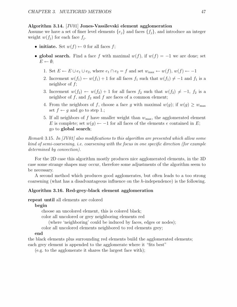
Algorithm 3.14. [JV01] Jones-Vassilevski element agglomerationAssume we have a set of finer level elements ej and faces fj, and introduce an integerweight w(fj) for each face fj.
• initiate. Set w(f)← 0 for all faces f ;
• global search. Find a face f with maximal w(f), if w(f) = −1 we are done; setE ← ∅;
1. Set E ← E ∪ e1 ∪ e2, where e1 ∩ e2 = f and set wmax ← w(f), w(f)← −1
2. Increment w(f1) ← w(f1) + 1 for all faces f1 such that w(f1) 6= −1 and f1 is aneighbor of f ;
3. Increment w(f2) ← w(f2) + 1 for all faces f2 such that w(f2) 6= −1, f2 is aneighbor of f , and f2 and f are faces of a common element;
4. From the neighbors of f , choose a face g with maximal w(g); if w(g) ≥ wmax
set f ← g and go to step 1.;
5. If all neighbors of f have smaller weight than wmax, the agglomerated elementE is complete; set w(g)← −1 for all faces of the elements e contained in E;go to global search;
Remark 3.15. In [JV01] also modifications to this algorithm are presented which allow somekind of semi-coarsening, i.e. coarsening with the focus in one specific direction (for exampledetermined by convection).
For the 2D case this algorithm mostly produces nice agglomerated elements, in the 3Dcase some strange shapes may occur, therefore some adjustments of the algorithm seem tobe necessary.
A second method which produces good agglomerates, but often leads to a too strongcoarsening (what has a disadvantageous influence on the h-independence) is the following.
Algorithm 3.16. Red-grey-black element agglomeration
repeat until all elements are coloredbegin
choose an uncolored element, this is colored black;color all uncolored or grey neighboring elements red
(where ‘neighboring’ could be induced by faces, edges or nodes);color all uncolored elements neighbored to red elements grey;
endthe black elements plus surrounding red elements build the agglomerated elements;each grey element is appended to the agglomerate where it “fits best”
(e.g. to the agglomerate it shares the largest face with);
Chapter 4
AMG Methods for the MixedProblem
We now come back to the original problem, i.e. to solve the saddle point system (2.29)
(A(w) BT
B −C
)(up
)=
(fg
),
using algebraic multigrid methods.
The Segregated Approach. A first possibility is the segregated approach. One coulduse an outer solver which iteratively decouples the equations — for example SIMPLE(Section 2.5.2), Uzawa (Section 2.5.3), or the preconditioner in Section 2.5.3.1 combinedwith a Krylov space method (section 2.5.1) — and then use an AMG method for theresulting scalar elliptic problems. This direction is followed e.g. in [GNR98], [Stu01a] or[SEKW01] and related publications.
A very nice property of this approach is the simplicity of its realization in a concretecomputer program. If components like scalar solvers are available they are easily assem-bled to a full solver for saddle point problems. One important subproblem here is thedevelopment of a fast and robust (multigrid-) solver for convection diffusion problems. Wewill not go into detail about that but refer to the literature, for example (without claimingcompleteness) [Reu95, BW97, OGWW98, YVB98, PTV00, DMS01, Reu02].
Unfortunately, sometimes (especially for Navier-Stokes resp. Oseen equations) the seg-regated approach has the drawback of a loss of optimality, i.e. an asymptotic complexityconsiderably larger than O(n) (n being the number of unknowns).
This is one of the reasons why we want to follow a different way. We will developAMG methods for the coupled problem. As the techniques of the previous chapter mostlyrequire positive definite systems, we have to adapt the ingredients to fit to our problemand develop some new methods.
48
CHAPTER 4. AMG METHODS FOR THE MIXED PROBLEM 49
4.1 Construction of the Coarse Level Systems
The first important part of our strategy is to avoid a mixture of velocity components andpressure on the coarse levels (which could occur if one just applies some “off-the-shelf”solver to the whole saddle point system), thus we choose a prolongation
P ll+1 =
(I ll+1
J ll+1
),
with
I ll+1 =
(I ll+1
I ll+1
)in 2D
resp.
I ll+1 =
I ll+1
I ll+1
I ll+1
in 3D,
whereI ll+1 : Rnl+1 → Rnl
is the prolongation matrix for one velocity component,
J ll+1 : Rml+1 → Rml
for pressure. We denote the corresponding restriction matrices by I l+1l , I l+1
l , J l+1l and use
I l+1l = (I ll+1)T , I l+1
l = (I ll+1)T , J l+1l = (J ll+1)T .
The system matrix on level l is denoted by(Al BT
l
Bl −Cl
).
the spaces for velocity and pressure unknown vectors by Ul := (Rnl)d and Ql
:= Rml andthe coarse function spaces by
Ul :=
v : ∃w ∈ Ul such that v = I12 I
23 . . . I
l−1l w
,
Ql :=p : ∃q ∈ Q
lsuch that p = J1
2J23 . . . J
l−1l q
.
Analogous to (2.19) we introduce the FE-AMG-isomorphisms φlU : Ul → Ul and φlQ :Ql→ Ql, and we will often identify elements of Ul and Ul, and Q
land Ql (see also Figure
4.1). In situations where it is not obvious which level the underline notation refers to, we
will use the operators φlU−1
and φlQ−1
explicitly.The system matrix on level l is constructed by Galerkin projection from the finer level
l − 1 as described in Section 3.1, we only have to take extra care of the stabilizing termsfor unstable elements as in Section 2.2.1.2 or convection as in Section 2.4.1.
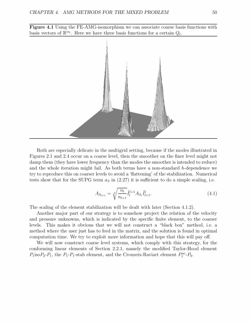
CHAPTER 4. AMG METHODS FOR THE MIXED PROBLEM 50
Figure 4.1 Using the FE-AMG-isomorphism we can associate coarse basis functions withbasis vectors of Rml. Here we have three basis functions for a certain Ql.
Both are especially delicate in the multigrid setting, because if the modes illustrated inFigures 2.1 and 2.4 occur on a coarse level, then the smoother on the finer level might notdamp them (they have lower frequency than the modes the smoother is intended to reduce)and the whole iteration might fail. As both terms have a non-standard h-dependence wetry to reproduce this on coarser levels to avoid a ‘flattening’ of the stabilization. Numericaltests show that for the SUPG term aS in (2.27) it is sufficient to do a simple scaling, i.e.
ASl+1= d
√nlnl+1
I l+1l ASi I
ll+1. (4.1)
The scaling of the element stabilization will be dealt with later (Section 4.1.2).Another major part of our strategy is to somehow project the relation of the velocity
and pressure unknowns, which is indicated by the specific finite element, to the coarserlevels. This makes it obvious that we will not construct a “black box” method, i.e. amethod where the user just has to feed in the matrix, and the solution is found in optimalcomputation time. We try to exploit more information and hope that this will pay off.
We will now construct coarse level systems, which comply with this strategy, for theconforming linear elements of Section 2.2.1, namely the modified Taylor-Hood elementP1isoP2-P1, the P1-P1-stab element, and the Crouzeix-Raviart element P nc
1 -P0.
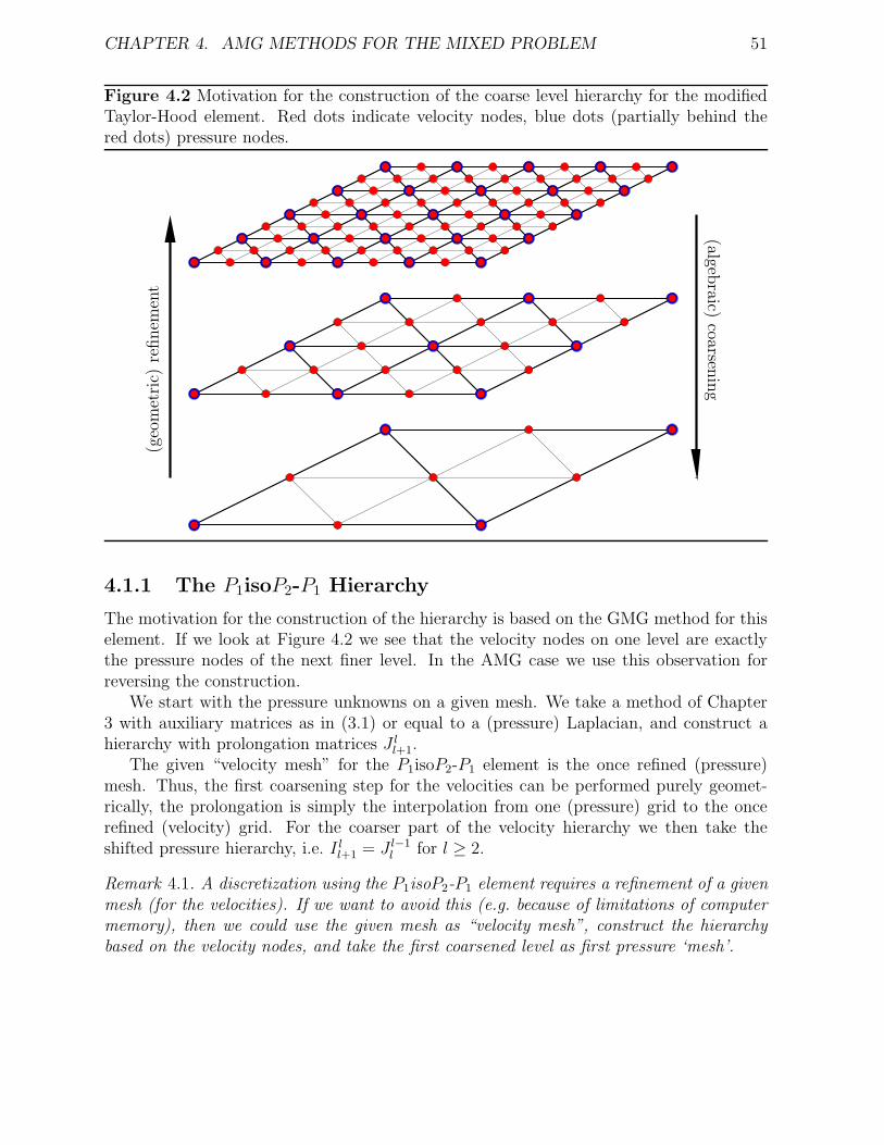
CHAPTER 4. AMG METHODS FOR THE MIXED PROBLEM 51
Figure 4.2 Motivation for the construction of the coarse level hierarchy for the modifiedTaylor-Hood element. Red dots indicate velocity nodes, blue dots (partially behind thered dots) pressure nodes.
PSfrag replacements
(geo
met
ric)
refinem
ent
(algebraic)
coarsenin
g
4.1.1 The P1isoP2-P1 Hierarchy
The motivation for the construction of the hierarchy is based on the GMG method for thiselement. If we look at Figure 4.2 we see that the velocity nodes on one level are exactlythe pressure nodes of the next finer level. In the AMG case we use this observation forreversing the construction.
We start with the pressure unknowns on a given mesh. We take a method of Chapter3 with auxiliary matrices as in (3.1) or equal to a (pressure) Laplacian, and construct ahierarchy with prolongation matrices J ll+1.
The given “velocity mesh” for the P1isoP2-P1 element is the once refined (pressure)mesh. Thus, the first coarsening step for the velocities can be performed purely geomet-rically, the prolongation is simply the interpolation from one (pressure) grid to the oncerefined (velocity) grid. For the coarser part of the velocity hierarchy we then take theshifted pressure hierarchy, i.e. I ll+1 = J l−1
l for l ≥ 2.
Remark 4.1. A discretization using the P1isoP2-P1 element requires a refinement of a givenmesh (for the velocities). If we want to avoid this (e.g. because of limitations of computermemory), then we could use the given mesh as “velocity mesh”, construct the hierarchybased on the velocity nodes, and take the first coarsened level as first pressure ‘mesh’.
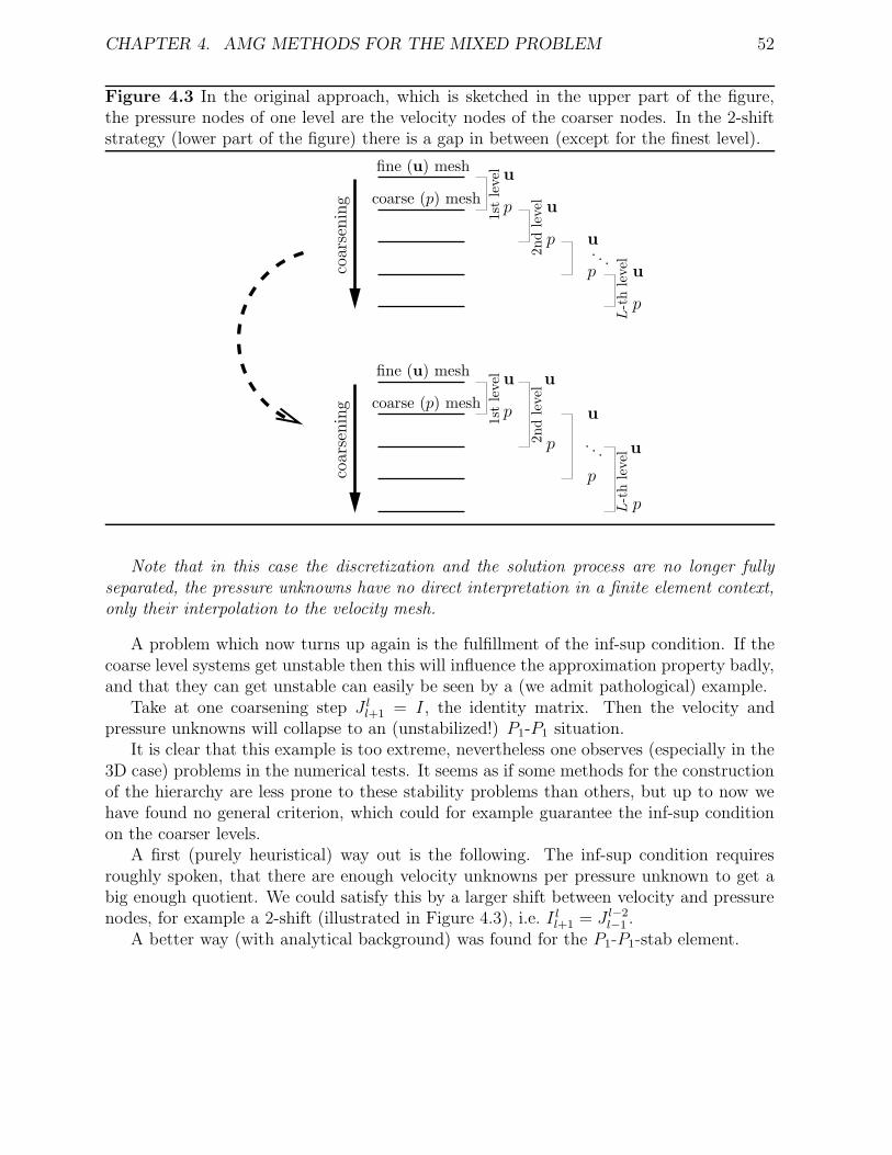
CHAPTER 4. AMG METHODS FOR THE MIXED PROBLEM 52
Figure 4.3 In the original approach, which is sketched in the upper part of the figure,the pressure nodes of one level are the velocity nodes of the coarser nodes. In the 2-shiftstrategy (lower part of the figure) there is a gap in between (except for the finest level).
PSfrag replacements
u
u
uu
u
u
u
u
p
p
p
p
p
p
p
p
coar
senin
gco
arse
nin
g
refinementfine (u) mesh
fine (u) mesh
coarse (p) mesh
coarse (p) mesh
1st
level
1st
level
2n
dle
vel
2n
dle
vel
. . .
. . .
L-t
hle
vel
L-t
hle
vel
Note that in this case the discretization and the solution process are no longer fullyseparated, the pressure unknowns have no direct interpretation in a finite element context,only their interpolation to the velocity mesh.
A problem which now turns up again is the fulfillment of the inf-sup condition. If thecoarse level systems get unstable then this will influence the approximation property badly,and that they can get unstable can easily be seen by a (we admit pathological) example.
Take at one coarsening step J ll+1 = I, the identity matrix. Then the velocity andpressure unknowns will collapse to an (unstabilized!) P1-P1 situation.
It is clear that this example is too extreme, nevertheless one observes (especially in the3D case) problems in the numerical tests. It seems as if some methods for the constructionof the hierarchy are less prone to these stability problems than others, but up to now wehave found no general criterion, which could for example guarantee the inf-sup conditionon the coarser levels.
A first (purely heuristical) way out is the following. The inf-sup condition requiresroughly spoken, that there are enough velocity unknowns per pressure unknown to get abig enough quotient. We could satisfy this by a larger shift between velocity and pressurenodes, for example a 2-shift (illustrated in Figure 4.3), i.e. I ll+1 = J l−2
l−1 .A better way (with analytical background) was found for the P1-P1-stab element.
CHAPTER 4. AMG METHODS FOR THE MIXED PROBLEM 53
4.1.2 The P1-P1-stab Hierarchy
Here the unknowns for the velocity components and for the pressure unknowns ‘live’ onthe same positions of the element, on the nodes. Thus it seems to be a good choice to takean arbitrary strategy from Chapter 3 for the construction of say I ll+1 and use J ll+1 = I ll+1
for the pressure.With some weak assumptions on I ll+1 it will be possible to show stability of the coarser
levels, what has to be specified first is the construction of the coarse level stabilizingmatrices Cl. For reasons which will become apparent in the proof of Lemma 4.3 we proposethe following. Set
C1 = C1, Cl+1 = J l+1l ClJ
ll+1, for l ≥ 1 (4.2)
and
Cl+1 =λmax(D−1
l Ml)
h2Cl+1, for l ≥ 1, (4.3)
where h is the discretization parameter of the finest level, Ml the Galerkin projection ofthe mass matrix M1 to level l, Dl the diagonal of one (component-) block of the Galerkinprojection of the vector-Laplacian ADl, and λmax(D−1
l Ml) denotes the largest eigenvalue ofD−1l Ml. For practical computation we will use very rough estimates for λmax(D−1
l Ml).Now we will show stability of the coarse level systems in the form
sup06=v∈Ul06=q∈Q
l
Bl(u, p; v, q)‖v‖ADl + ‖q‖Ml
≥ ζ (‖u‖ADl + ‖p‖Ml) ∀(u, p) ∈ Ul ×Ql
, (4.4)
with a constant ζ and
Bl(u, p; v, q) = uTADlv + pTBlv + uTBTl q − pTClq.
For this we use the ideas given in [FS91, FHS93] and just ‘translate’ them to our algebraicsetting.
Remark 4.2. Condition (4.4) is the inf-sup condition needed by the theorem of Babuska andAziz [BA72], [Bra97, theorem 3.6]. It would be a consequence of the LBB condition neededby Theorem 2.2, the reverse does obviously not hold.
The main point of the stability analysis will be the following lemma, which has beenproven in [Ver84a] for the geometric case.
CHAPTER 4. AMG METHODS FOR THE MIXED PROBLEM 54
Lemma 4.3. Assume that for all elements τj ∈ Th the diameter hτj fulfills
αh ≤ hτj ≤ αh, (4.5)
with positive constants α and α and the discretization parameter h, and assume furtherthat ADl is symmetric and of essentially positive type (see Definition 3.5) and that for allvl ∈ Ul we can find Πl+1
l vl ∈ Ul+1 such that
‖vl − I ll+1Πl+1l vl‖2
Dl≤ β1‖vl‖2
ADl, (4.6)
with some constant β1.Then for all levels l ∈ 1, . . . , L there exist positive cl and dl such that
sup06=v∈Ul
vBTl p
‖v‖ADl≥ cl‖p‖Ml
− dl(pTClp
) 12 ∀p ∈ Ql. (4.7)
Proof. Since in the course of this proof we will have to distinguish between the elementsof Ul, Ql
and their representatives in Ul, Ql we will again use the “underline-notation”.Obviously
‖xl‖2Ml≤ λmax(D−1
l Ml)‖xl‖2Dl
for any xl, hence‖vl − I ll+1Πl+1
l vl‖2Ml≤ λmax(D−1
l Ml)β1‖vl‖2ADl
,
therefore there exists Πl+1l vl ∈ Ul+1, such that
‖vl − Πl+1l vl‖2
0 ≤ λmax(D−1l Ml)β1‖vl‖2
1. (4.8)
Because ADl is essentially positive definite we know from Lemma 3.7 that
2
ωxTDlx ≥ xTADlx. (4.9)
Because of
‖I ll+1Πl+1l vl‖ADl − ‖vl‖ADl ≤ ‖I
ll+1Πl+1
l vl − vl‖ADl
≤√
2
ω‖I ll+1Πl+1
l vl − vl‖Dl
≤√
2β1
ω‖vl‖ADl
we see that
‖I ll+1Πl+1l vl‖ADl ≤
(1 +
√2β1
ω
)
︸ ︷︷ ︸=:β2
‖vl‖ADl . (4.10)
CHAPTER 4. AMG METHODS FOR THE MIXED PROBLEM 55
We will now show by induction that on all levels l we can estimate
(div wl, pl) ≥ cl‖wl‖1‖pl‖0 − dl‖wl‖1
(pTlClpl
)1/2
for all pl ∈ Ql. (4.11)
For that we assume that (4.11) is valid on some level l (for l = 1 it is valid because therewe are in the geometric case). Set wl+1 = Πl+1
l wl. Then
(div wl+1, pl+1) = (div(wl+1 −wl), pl+1) + (div wl, pl+1)
= (wl −wl+1,∇pl+1) + (div wl, pl+1)
≥ −(∑
j
h−2τj‖wl −wl+1‖2
0,τj
)1/2
·(∑
j
h2τj‖∇pl+1‖2
0,τj
)1/2
+ (div wl, pl+1).
(4.12)
We will now derive estimates for the terms in the last inequality. Because of (4.5) and(4.8) we know that
∑
j
h−2τj‖wl −wl+1‖2
0,τj≤ (αh)−2‖wl −wl+1‖2
0
≤ β1
α2
λmax(D−1l Ml)
h2‖wl‖2
1,
with the definition of C1, Cl+1, and Cl+1 we get
∑
j
h2τj‖∇pl+1‖2
0,τj= pT
l+1Cl+1pl+1
=h2
λmax(D−1l Ml)
pTl+1Cl+1pl+1
,
and because of (4.11) we can derive that
(div wl, pl+1) ≥ cl‖wl‖1‖pl+1‖0 − dl‖wl‖1
(pTl+1J l+1l ClJ
ll+1pl+1
)1/2
= cl‖wl‖1‖pl+1‖0 − dl√
λmax(D−1l Ml)
λmax(D−1l−1Ml−1)
‖wl‖1
(pTl+1Cl+1pl+1
)1/2
.
Combining these results with (4.12) gives
(div wl+1, pl+1) ≥ −√β1
α‖wl‖1
(pTl+1Cl+1pl+1
)1/2
+ (div wl, pl+1)
≥ −(√
β1
α+ dl
√λmax(D−1
l Ml)
λmax(D−1l−1Ml−1)
)· ‖wl‖1
(pTl+1Cl+1pl+1
)1/2
+ cl‖pl+1‖0‖wl‖1.
CHAPTER 4. AMG METHODS FOR THE MIXED PROBLEM 56
With (4.10) we get
(div wl+1, pl+1)
‖wl+1‖1≥ β−1
2
(div wl+1, pl+1)
‖wl‖1
≥ cl/β2‖pl+1‖0
−(√
β1
β2α+dlβ2
√λmax(D−1
l Ml)
λmax(D−1l−1Ml−1)
)·(pTl+1Cl+1pl+1
)1/2
,
hence, with
cl+1 := cl/β2 and
dl+1 :=
√β1
β2α+dlβ2
√λmax(D−1
l Ml)
λmax(D−1l−1Ml−1)
we complete the proof.
We are now ready to prove stability.
Theorem 4.4. Suppose that the assumptions of Lemma 4.3 hold. Then
sup06=v∈Ul06=q∈Q
l
Bl(u, p; v, q)‖v‖ADl + ‖q‖Ml
≥ ζ(‖u‖ADl + ‖p‖Ml
)∀(u, p) ∈ Ul ×Ql
, (4.13)
with some ζ > 0 (where ζ may depend on l).
Proof. Choose (for given u and p) w ∈ Ul such that the supremum in Lemma 4.3 isattained and that ‖w‖ADl = ‖p‖Ml
. Now
Bl(u, p; w, 0) = uTADlw + pTBlwLemma 4.3≥ −‖u‖ADl‖w‖ADl + cl‖w‖ADl‖p‖Ml
− dl‖w‖ADl(pTClp
)1/2
= −‖u‖ADl‖p‖Ml+ cl‖p‖2
Ml− dl‖p‖Ml
(pTClp
)1/2
xy≤x2ε +εy2
2≥ − 1
2ε‖u‖2
ADl− ε
2‖p‖2
Ml+ cl‖p‖2
Ml− dl
2εpTClp−
dlε
2‖p‖2
Ml
= −θ1‖u‖2ADl
+ θ2‖p‖2Ml− θ3p
TClp,
where cl and dl are the constants given by Lemma 4.3 and θ1 := 12ε
, θ2 := cl − ε2(1 + dl),
and θ3 := dl2ε
are positive constants if we choose 0 < ε < 2cl1+dl
.
We now take (v, q) = (u + ϑw,−p) with a parameter ϑ and get
Bl(u, p; v, q) = Bl(u, p; u + ϑw,−p)= Bl(u, p; u,−p) + ϑBl(u, p; w, 0)
≥ ‖u‖2ADl
+ pTClp− ϑθ1‖u‖2ADl
+ ϑθ2‖p‖2Ml− ϑθ3p
TClp.
CHAPTER 4. AMG METHODS FOR THE MIXED PROBLEM 57
We choose 0 < ϑ < min(
1θ1, 1θ3
), resulting in
Bl(u, p; v, q) ≥ θ4
(‖u‖2
ADl+ ‖p‖2
Ml
),
with some appropriate constant θ4. Since
‖v‖ADl + ‖q‖Ml= ‖u + ϑw‖ADl + ‖p‖Ml
≤ ‖u‖ADl + ϑ‖w‖ADl + ‖p‖Ml
≤ (1 + ϑ)(‖u‖ADl + ‖p‖Ml
)
we can sum up
Bl(u, p; v, q)‖v‖ADl + ‖q‖Ml
≥ θ5
‖u‖2ADl
+ ‖p‖2Ml
‖u‖ADl + ‖p‖Ml
≥ θ5
2
(‖u‖ADl + ‖p‖Ml
)
(where θ5 = θ4/(1 + ϑ)).
Now the question remains, how restrictive assumption (4.6) is. For the Ruge-Stubenprolongation (3.14) we have discussed a similar property in Theorems 3.8 and 3.9. Sinceproperty (3.16) in Theorem 3.9 is fulfilled if every F node is strongly coupled to a Cnode (which is the case for Algorithm 3.10 with the modifications concerning the stronglynegative couplings), we get that (3.17) holds, i.e.
‖eF − P FC eC‖2
Dl,F≤ c‖e‖2
ADl.
Thus, (4.6) is fulfilled for
Πl+1l vl = Πl+1
l
(vFvC
)= vC .
As the methods presented in Sections 4.1.1 and 4.1.2 were more or less tailor-madefor mixed elements constructed from linear elements, the question on generalizations couldarise. One possibility could be the strategy developed by John, Knobloch, Matthies and To-biska in [JKMT02] for geometric multigrid methods. There the first fine-to-coarse transferis an element-type transfer, in their case from higher-order elements (which possess prefer-able discretization properties) to the P nc
1 -P0 element (which possesses preferable propertiesin connection with the linear solver). Adapting this idea to our needs, we could discretizeusing an arbitrary mixed-element, transfer to the P1-P1-stab element and then use thehierarchy presented above. To us this seems to be a good possibility, however we have notmade any numerical experiences in this direction up to now.
Another general method is the application of the element agglomerating AMGe tech-nique (Section 3.2.2.2) on mixed elements. We exemplarily present this for the Crouzeix-Raviart element in the following section.
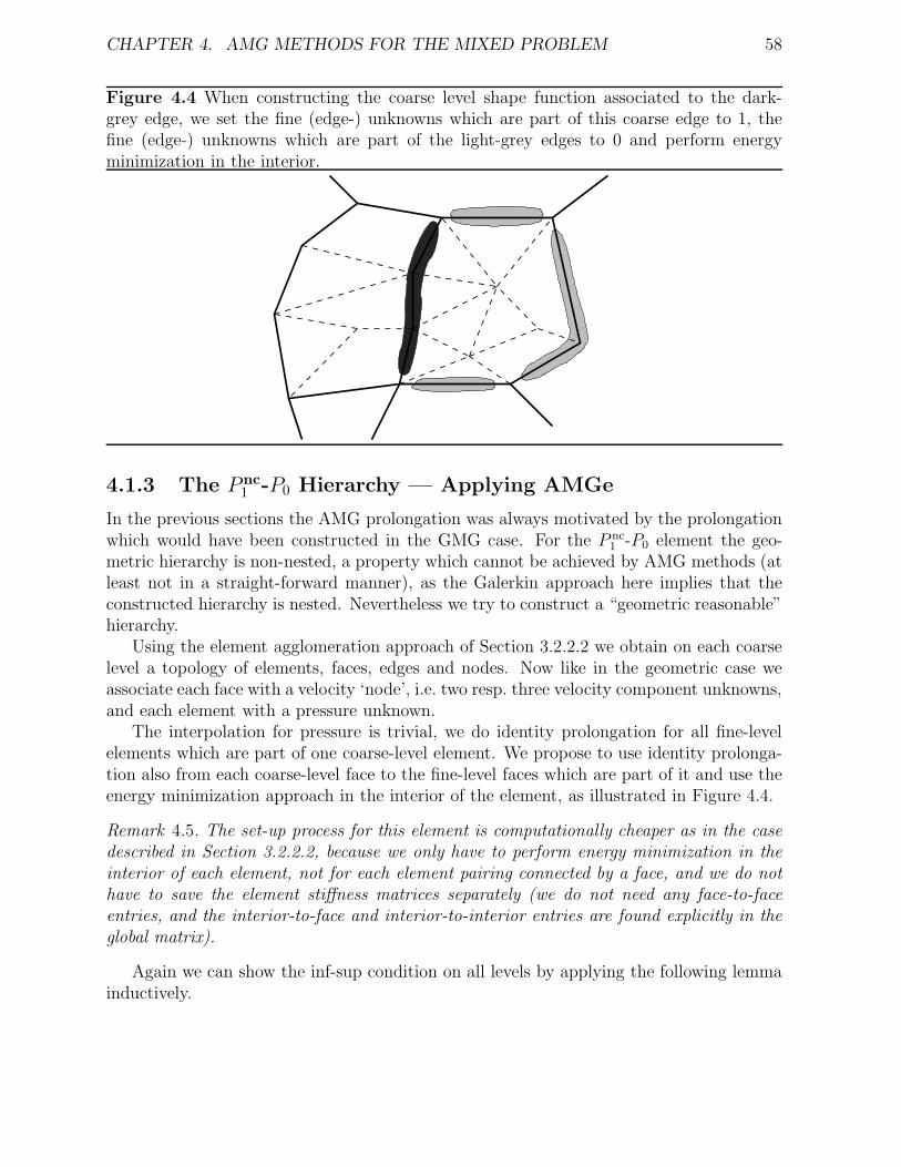
CHAPTER 4. AMG METHODS FOR THE MIXED PROBLEM 58
Figure 4.4 When constructing the coarse level shape function associated to the dark-grey edge, we set the fine (edge-) unknowns which are part of this coarse edge to 1, thefine (edge-) unknowns which are part of the light-grey edges to 0 and perform energyminimization in the interior.
4.1.3 The P nc1 -P0 Hierarchy — Applying AMGe
In the previous sections the AMG prolongation was always motivated by the prolongationwhich would have been constructed in the GMG case. For the P nc
1 -P0 element the geo-metric hierarchy is non-nested, a property which cannot be achieved by AMG methods (atleast not in a straight-forward manner), as the Galerkin approach here implies that theconstructed hierarchy is nested. Nevertheless we try to construct a “geometric reasonable”hierarchy.
Using the element agglomeration approach of Section 3.2.2.2 we obtain on each coarselevel a topology of elements, faces, edges and nodes. Now like in the geometric case weassociate each face with a velocity ‘node’, i.e. two resp. three velocity component unknowns,and each element with a pressure unknown.
The interpolation for pressure is trivial, we do identity prolongation for all fine-levelelements which are part of one coarse-level element. We propose to use identity prolonga-tion also from each coarse-level face to the fine-level faces which are part of it and use theenergy minimization approach in the interior of the element, as illustrated in Figure 4.4.
Remark 4.5. The set-up process for this element is computationally cheaper as in the casedescribed in Section 3.2.2.2, because we only have to perform energy minimization in theinterior of each element, not for each element pairing connected by a face, and we do nothave to save the element stiffness matrices separately (we do not need any face-to-faceentries, and the interior-to-face and interior-to-interior entries are found explicitly in theglobal matrix).
Again we can show the inf-sup condition on all levels by applying the following lemmainductively.
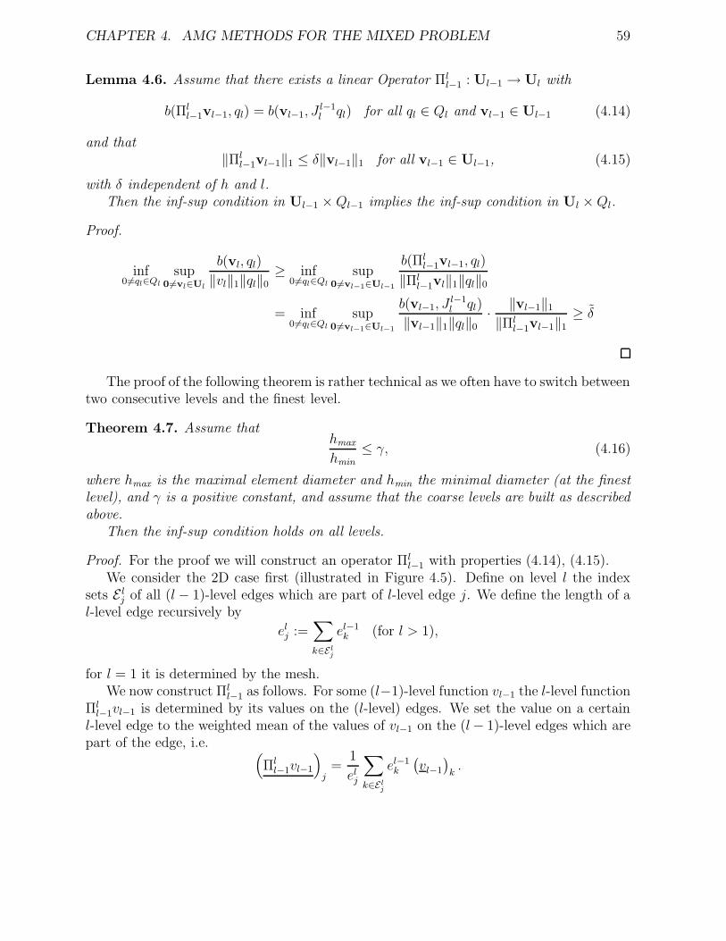
CHAPTER 4. AMG METHODS FOR THE MIXED PROBLEM 59
Lemma 4.6. Assume that there exists a linear Operator Πll−1 : Ul−1 → Ul with
b(Πll−1vl−1, ql) = b(vl−1, J
l−1l ql) for all ql ∈ Ql and vl−1 ∈ Ul−1 (4.14)
and that‖Πl
l−1vl−1‖1 ≤ δ‖vl−1‖1 for all vl−1 ∈ Ul−1, (4.15)
with δ independent of h and l.Then the inf-sup condition in Ul−1 ×Ql−1 implies the inf-sup condition in Ul ×Ql.
Proof.
inf06=ql∈Ql
sup06=vl∈Ul
b(vl, ql)
‖vl‖1‖ql‖0≥ inf
06=ql∈Qlsup
06=vl−1∈Ul−1
b(Πll−1vl−1, ql)
‖Πll−1vl‖1‖ql‖0
= inf06=ql∈Ql
sup06=vl−1∈Ul−1
b(vl−1, Jl−1l ql)
‖vl−1‖1‖ql‖0
· ‖vl−1‖1
‖Πll−1vl−1‖1
≥ δ
The proof of the following theorem is rather technical as we often have to switch betweentwo consecutive levels and the finest level.
Theorem 4.7. Assume thathmax
hmin≤ γ, (4.16)
where hmax is the maximal element diameter and hmin the minimal diameter (at the finestlevel), and γ is a positive constant, and assume that the coarse levels are built as describedabove.
Then the inf-sup condition holds on all levels.
Proof. For the proof we will construct an operator Πll−1 with properties (4.14), (4.15).
We consider the 2D case first (illustrated in Figure 4.5). Define on level l the indexsets E lj of all (l − 1)-level edges which are part of l-level edge j. We define the length of al-level edge recursively by
elj :=∑
k∈E lj
el−1k (for l > 1),
for l = 1 it is determined by the mesh.We now construct Πl
l−1 as follows. For some (l−1)-level function vl−1 the l-level functionΠll−1vl−1 is determined by its values on the (l-level) edges. We set the value on a certain
l-level edge to the weighted mean of the values of vl−1 on the (l− 1)-level edges which arepart of the edge, i.e. (
Πll−1vl−1
)j
=1
elj
∑
k∈E lj
el−1k
(vl−1
)k.
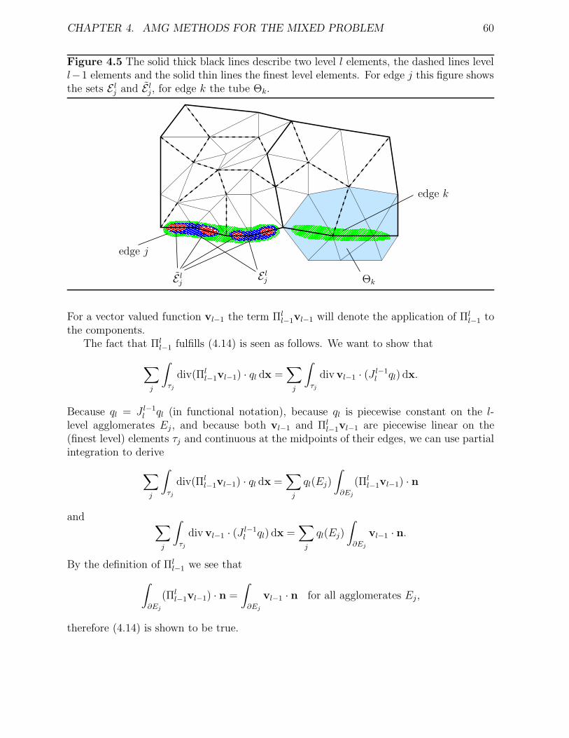
CHAPTER 4. AMG METHODS FOR THE MIXED PROBLEM 60
Figure 4.5 The solid thick black lines describe two level l elements, the dashed lines levell−1 elements and the solid thin lines the finest level elements. For edge j this figure showsthe sets E lj and E lj, for edge k the tube Θk.
PSfrag replacements
edge j
E lj E lj Θk
edge k
For a vector valued function vl−1 the term Πll−1vl−1 will denote the application of Πl
l−1 tothe components.
The fact that Πll−1 fulfills (4.14) is seen as follows. We want to show that
∑
j
∫
τj
div(Πll−1vl−1) · ql dx =
∑
j
∫
τj
div vl−1 · (J l−1l ql) dx.
Because ql = J l−1l ql (in functional notation), because ql is piecewise constant on the l-
level agglomerates Ej, and because both vl−1 and Πll−1vl−1 are piecewise linear on the
(finest level) elements τj and continuous at the midpoints of their edges, we can use partialintegration to derive
∑
j
∫
τj
div(Πll−1vl−1) · ql dx =
∑
j
ql(Ej)
∫
∂Ej
(Πll−1vl−1) · n
and ∑
j
∫
τj
div vl−1 · (J l−1l ql) dx =
∑
j
ql(Ej)
∫
∂Ej
vl−1 · n.
By the definition of Πll−1 we see that
∫
∂Ej
(Πll−1vl−1) · n =
∫
∂Ej
vl−1 · n for all agglomerates Ej,
therefore (4.14) is shown to be true.
CHAPTER 4. AMG METHODS FOR THE MIXED PROBLEM 61
What remains to show is (4.15). This will be done by the introduction of an auxiliaryoperator Πl
l−1 on the finer level Ul−1, which fulfills (4.15) and which is identical to Πll−1 on
the coarse edges. Because we use energy minimization for the interpolation in the interiorof agglomerates we will then be able to estimate Πl
l−1 by Πll−1 which will complete the
proof.We define Πl
l−1 : Ul−1 → Ul−1 by
Πl
l−1(vl−1)j :=
(vl−1)j if j /∈ E lk for all k,(
Πll−1vl−1
)k
if j ∈ E lk for a certain k.
Note that Πll−1vl−1 still ‘lives’ on level l−1, only the values at the l-level faces are averaged.
We try to find an upper bound for∣∣∣vl−1 − Πl
l−1vl−1
∣∣∣1. Define E lj the index set of all
finest-level edges which lie on coarse edge j. Set v1 (component of finest-level functionv1 ∈ U1) equal to vl−1 − Πl
l−1vl−1 on all (finest level) degrees of freedom in⋃j E lj and zero
on all other (finest level) degrees of freedom. Then because of the energy minimization inthe prolongation
∫
G∇(vl−1 − Πl
l−1vl−1
)∇(vl−1 − Πl
l−1vl−1
)dx ≤
∫
G∇v1∇v1 dx
≤∑
l-leveledges j
∫
Θj
∇v1∇v1 dx,(4.17)
where Θj is the tube of (finest level) elements which share a point or edge with l-level edgenumber j.
For a (finest level) triangle PQR and the basis function ϕPQ, which is equal to 1 at themidpoint of PQ and zero at the midpoints of QR and RP one can easily calculate
∫
PQR
∇ϕPQ∇ϕPQ dx =|PQ|2
A(PQR),
where A(PQR) denotes the area of the triangle PQR. Now with
c1 := maxτj
(length of longest edge of τj)2
A(τj)
CHAPTER 4. AMG METHODS FOR THE MIXED PROBLEM 62
Figure 4.6 Detail of Figure 4.5, the set S l−1m .
PSfrag replacements
(φ1U−1vl−1)j
(φ1U−1vl−1)k
vl−1(a1)
vl−1(a2)r1
r2
r3
we get
∫
Θj
∇v1∇v1 dx ≤ c1
∑
s∈E lj
((v1)s)2
= c1
∑
s∈E lj
1∑k∈E lj ek
∑
k∈E lj
ek
((φ1U−1vl−1
)s−(φ1U−1vl−1
)k
)
2
≤ c1
∑k∈E lj
e2k
(∑k∈E lj ek
)2
∑
s∈E lj ,k∈E lj
((φ1U−1vl−1
)s−(φ1U−1vl−1
)k
)2
≤ c1
∑
s∈E lj ,k∈E lj
((φ1U−1vl−1
)s−(φ1U−1vl−1
)k
)2
≤ c1
∑
s∈E lj ,k∈E lj
((vl−1
)s−(vl−1
)k
)2,
(4.18)
where φ1U−1v is the representation of a coarse function v on U1 as in Section 4.1.
We note that ∇vl−1 is constant on each finest level element. Therefore we can derivethe following estimate (illustrated in Figure 4.6). Assume that the (l−1)-level edges j andk share the node m. We denote the set of all finest level elements which share the nodem with S l−1
m , its index set with S l−1m (where we assume w.l.o.g. S l−1
m = 1, 2, . . . , i + 1).For each element τe in S l−1
m we denote the edge-vector of the edge not connected to m (“indirection” j → k) with re.
CHAPTER 4. AMG METHODS FOR THE MIXED PROBLEM 63
Then
(vl−1)k − (vl−1)j = ((vl−1)k − vl−1(a1)) + (vl−1(a1)− vl−1(a2)) + . . .+ (vl−1(ai)− (vl−1)j)
=1
2
(∇vl−1|τ1 · r1 + . . .+∇vl−1|τi+1
· ri+1
)
≤ 1
2
(√∇vl−1|τ1 · ∇vl−1|τ1 |r1|+ . . .+
√∇vl−1|τi+1
· ∇vl−1|τi+1|ri+1|
),
where a1,. . . ,ai are finest level edge midpoints as in Figure 4.6, thus (using the algebraic-geometric mean inequality)
((vl−1)k − (vl−1)j
)2 ≤ i + 1
4
[|r1|2 (∇vl−1|τ1)2 + . . .+ |ri+1|2
(∇vl−1|τi+1
)2]
≤ c2
∫
Sl−1m
∇vl−1∇vl−1 dx.(4.19)
We apply this estimate to the last term in (4.18), which is done directly for those (l − 1)-level edges s and k which share a node. For all others we have to build a chain of connectingedges.
This leads to ∫
Θl
∇v1∇v1 dx ≤ c3
∫
Θl
∇vl−1∇vl−1 dx.
Now because of (4.17) we get
∥∥∥vl−1 − Πll−1vl−1
∥∥∥1≤ c4‖vl−1‖1,
thus ∥∥∥Πll−1vl−1
∥∥∥1≤ (1 + c4)‖vl−1‖1.
Because we use energy minimization for the interpolation in the interior of coarse agglom-erates, I l−1
l Πll−1vl−1 has minimal energy amongst all l−1-level functions which are identical
to it on the l-level edges, therefore
∥∥Πll−1vl−1
∥∥1≤ c5
∥∥∥Πll−1vl−1
∥∥∥1≤ c5(1 + c4)‖vl−1‖1. (4.20)
3D case. For 3D tetrahedral elements we replace c1 in (4.18) by c1hj,max, where hj,max
is the maximal element height in tube Θj, and c2 in (4.19) by c2/hj,min, where hj,min is theminimal element height in this tube. Then because of (4.16) the argumentation remainsunchanged, only the scaling argument is based on the (finest level) tetrahedron PQRS
∫
PQRS
∇ϕPQR∇ϕPQR dx =A(PQR)2
V (PQRS),
where V (PQRS) is the volume of the tetrahedron.
CHAPTER 4. AMG METHODS FOR THE MIXED PROBLEM 64
4.2 Smoothers
Now that the coarse levels are constructed we need smoothers for the coupled systems onall levels. We will give a short overview of some possibilities thereof, and then go intodetail for the two methods we primarily use, namely Braess-Sarazin and Vanka smoothers.
To the author’s knowledge there is no smoothing-theory for algebraic multigrid methodsfor fundamentally indefinite systems, i.e. not just disturbed positive definite systems. Weadmit that we have no contributions in this direction either, thus we will apply the followingheuristic.
Hypothesis 4.8. If a smoother for a saddle point problem performs ‘well’ in the geometricmultigrid situation, then it will also do so in the algebraic multigrid situation.
In the light of this heuristic an important quality factor for the smoothers is the smooth-ing rate, which we introduced in Section 3.1.1.
Note that the parts of the following sections which concern the analysis of the smoothersall base on geometric multigrid and on a symmetric system matrix, i.e. the Stokes case.As the smoothers (mostly) operate on one single level, we will drop the level index in thefollowing sections.
4.2.1 Standard Smoothers for the Squared System
As the system we are interested in is indefinite, it is not possible to apply standard smooth-ing methods (e.g. Richardson, Jacobi, Gauss-Seidel) at first. This could be overcome byapplying those smoothers to the squared (and thus symmetric, positive definite) system
(A BT
B −C
)T (A BT
B −C
)(up
)=
(A BT
B −C
)T (fg
).
This idea is used for example in [Ver84b] (here the second block row is scaled by 1/h2) or[Bre93], both use Richardson iterations on the squared system which can be shown to lead
to a (geometric) smoothing rate η(m) of order O(
1√m
).
4.2.2 Transforming Smoothers
This class of smoothers was introduced by Wittum in [Wit89, Wit90] and is based on ageneralization of the factorization for the SIMPLE scheme (2.31), namely
K =
(A 0B E
)
︸ ︷︷ ︸=:K1
(I A−1BT
0 −E−1S
)
︸ ︷︷ ︸=:K2
with an arbitrary positive definite matrix E (in (2.31) we had E = S). The idea isto transform K by a multiplication from the right with K−1
2 to K1, and then to find
CHAPTER 4. AMG METHODS FOR THE MIXED PROBLEM 65
smoothers for the block-triangular K1 (in [Wit89] it is shown that they only have to fulfillthe smoothing property for the diagonal blocks A and E). Suggested choices for E areS or As (the scalar, i.e. pressure variant of A). The latter does not lead to a practicablemethod at first, (heuristic) considerations about commuting operators (similarly as inSection 2.5.3.1) are needed, but we will not go into detail here.
In [Wit90] damped Jacobi, Gauss-Seidel and ILU smoothers are used for the trans-
formed system. For damped Jacobi a smoothing rate of order O(
1√m
)is shown, for the
other two only O(
lnm√m
), but it is stated that in numerical practice a rate of order O
(1m
)
is observed for the ILU transforming smoother.
4.2.3 Braess-Sarazin Smoother
This smoother consists of the application of the inexact symmetric Uzawa algorithm (2.36),which we repeat here for convenience of reading:
A(uk+1 − uk) = f − Auk − BTpk, (4.21a)
S(pk+1 − pk) = Buk+1 − Cpk − g, (4.21b)
A(uk+1 − uk+1) = −BT (pk+1 − pk), (4.21c)
where now S is a preconditioner for the inexact Schur-complement C +BA−1BT .The smoothing property with a rate of O
(1m
)for this method was shown in [BS97]
under the assumption that the pressure update (4.21b) is done (almost) exactly, i.e. S ≡C + BA−1BT . In [Zul00] we find that the same behavior can be obtained under weakerassumptions.
Theorem 4.9. [Zul00, theorem 2] Let A and C be symmetric positive semi-definite ma-trices, A and S symmetric positive definite matrices, satisfying
A ≥ A, (4.22a)
S ≤C +BA−1BT , (4.22b)
C +BA−1BT ≤ (1 + β)S, (4.22c)
and‖A‖`2 ≤ c1h
−2, ‖A−1‖`2 ≤ c2h2, ‖B‖`2 ≤ c3h
−2, ‖C‖`2 ≤ c4h−2.
Then the smoothing property‖KSm‖`2 ≤ η(m)h−2
is satisfied with
η(m) = max
[(1 + ρ)ρm−1,
(m− 1)m−1
mm
], with ρ = β +
√β2 + β.
CHAPTER 4. AMG METHODS FOR THE MIXED PROBLEM 66
For β < 1/3 we get ρ < 1, thus the second term in the maximum will dominate for mlarge enough. As this term can be bounded by
(m− 1)m−1
mm=
(1− 1
m
)m
(m− 1)≤ 1
e(m− 1)for m > 1
we get the smoothing rate O( 1m
) mentioned above.
We use an (inner) AMG method for C + BˆA−1BT as S−1, where
ˆA = α ·D, with the
diagonal D of A, (damped Jacobi iteration; thus we are able to explicitly construct thematrix, what is needed for the AMG method). For A we want to use some damped SSOR(or SSUR) iteration, i.e.
A = δ(D + γE)D−1(D + γF ),
where E is the lower left triangular part (with zero diagonal), and F the upper righttriangular part (with zero diagonal) of A, and δ and γ are some parameters. The followingcorollary shows the impact of (4.22) on the choice of the parameters α, δ and γ, under theassumption that A is an M-matrix. For essentially positive type matrices similar results asthe following could be shown, for simplicity of presentation we will not go into the detailsbut restrict ourselves to the M-matrix case.
Corollary 4.10. Assume that
• A is an M-matrix, that
• A and S are constructed as indicate above, and that
• the estimate
(1− ηk)S ≤ C +1
αBD−1BT ≤ S, (4.23)
where η < 1 is the convergence rate of the multigrid method and k the number ofiterations, is valid,
and define
ω := sup06=p∈ m
pTCp
pTBD−1BTp.
Then (4.22) is fulfilled if
δ(1− γ) ≥ 2, (4.24a)
δ(1 + γ + ρ2γ2) ≤ α1− ηk
1 + ωηk, and (4.24b)
(1 + β)δ(1− γ) ≥ α (4.24c)
hold, where
ρ :=maxi aiimini aii
.
CHAPTER 4. AMG METHODS FOR THE MIXED PROBLEM 67
Proof. It is easily seen that
αD ≤ (1 + β)δ(D + γF + γE + γ2ED−1F )
is a sufficient condition for (4.22c), which is certainly fulfilled for (4.24c).Analogously one can show that (4.24a) is sufficient for (4.22a).What remains is (4.22b), a sufficient condition would be
δ(D + γE + γF + γ2ED−1F ) ≤ α1− ηk
1 + ωηkD.
To estimate the last term on the left hand side we split as follows
xTED−1Fx
xTx≤ ‖ED−1/2‖∞‖D−1/2F‖∞
and calculate
‖ED−1/2‖∞ = maxi
(i−1∑
j=1
|aij|√ajj
)≤ ρmax
i
(i−1∑
j=1
|aij|√aii
)≤ ρ‖D1/2‖∞
and similarly‖D−1/2F‖∞ ≤ ‖D1/2‖∞.
Now we get for all xxTED−1Fx
xTx≤ ρ‖D‖∞ ≤ ρ2 xTDx
xTx
and summing up
D + γE + γF + γ2ED−1F = (1− γ)D + γA+ γ2ED−1F
≤ (1 + γ + ρ2γ2)D.
Thus we get the sufficient condition for (4.22b)
δ(1 + γ + ρ2γ2) ≤ α1− ηk
1 + ωηk.
Remark 4.11. Condition (4.23) is fulfilled e.g. if S originates in a convergent, symmetricmultigrid method and some additional (but weak) assumption hold (for example that thecoarse level systems are constructed with the Galerkin approach), for details we refer e.g.to [Hac93].
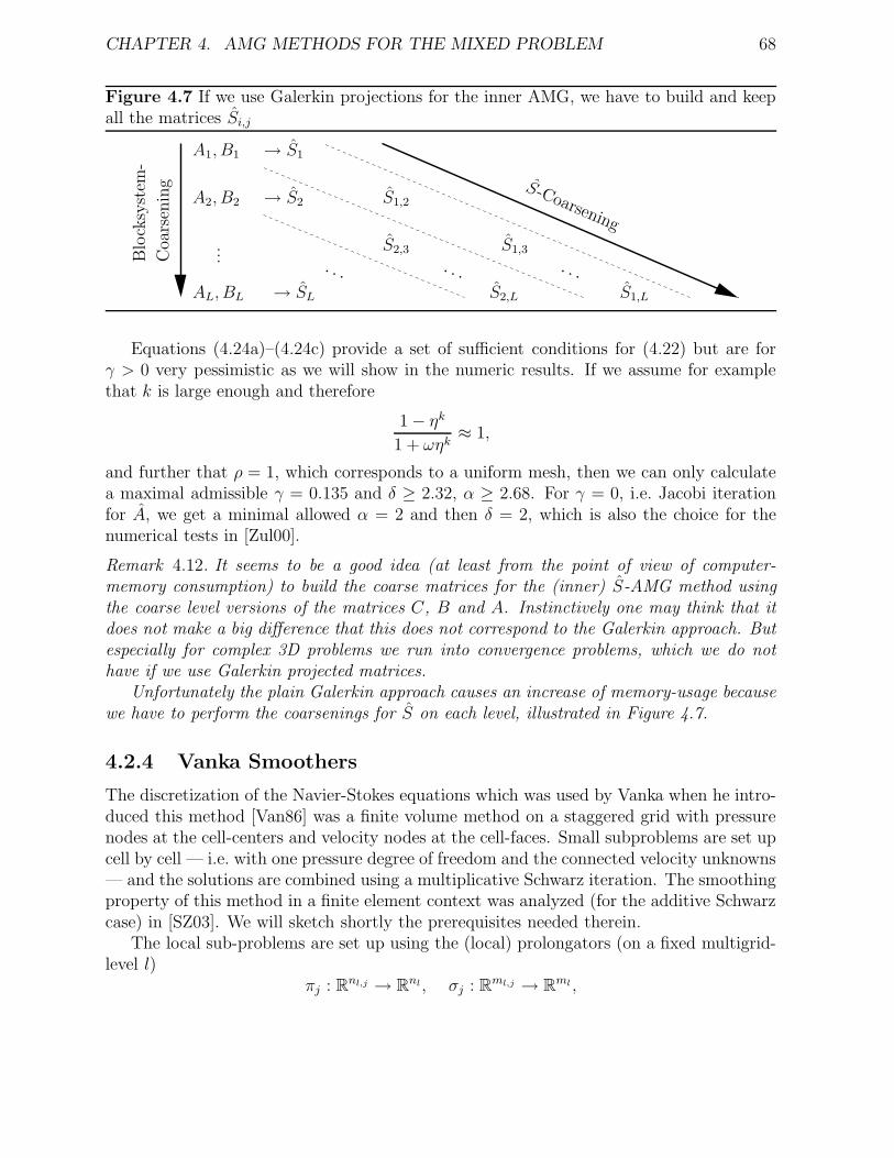
CHAPTER 4. AMG METHODS FOR THE MIXED PROBLEM 68
Figure 4.7 If we use Galerkin projections for the inner AMG, we have to build and keepall the matrices Si,j
PSfrag replacements
A1, B1
A2, B2
AL, BL
→ S1
→ S2
→ SL
S1,2
S1,3
S1,L
S2,3
S2,L
... · · ·· · ·· · ·
Blo
cksy
stem
-
Coa
rsen
ing S-Coarsening
Equations (4.24a)–(4.24c) provide a set of sufficient conditions for (4.22) but are forγ > 0 very pessimistic as we will show in the numeric results. If we assume for examplethat k is large enough and therefore
1− ηk1 + ωηk
≈ 1,
and further that ρ = 1, which corresponds to a uniform mesh, then we can only calculatea maximal admissible γ = 0.135 and δ ≥ 2.32, α ≥ 2.68. For γ = 0, i.e. Jacobi iterationfor A, we get a minimal allowed α = 2 and then δ = 2, which is also the choice for thenumerical tests in [Zul00].
Remark 4.12. It seems to be a good idea (at least from the point of view of computer-memory consumption) to build the coarse matrices for the (inner) S-AMG method usingthe coarse level versions of the matrices C, B and A. Instinctively one may think that itdoes not make a big difference that this does not correspond to the Galerkin approach. Butespecially for complex 3D problems we run into convergence problems, which we do nothave if we use Galerkin projected matrices.
Unfortunately the plain Galerkin approach causes an increase of memory-usage becausewe have to perform the coarsenings for S on each level, illustrated in Figure 4.7.
4.2.4 Vanka Smoothers
The discretization of the Navier-Stokes equations which was used by Vanka when he intro-duced this method [Van86] was a finite volume method on a staggered grid with pressurenodes at the cell-centers and velocity nodes at the cell-faces. Small subproblems are set upcell by cell — i.e. with one pressure degree of freedom and the connected velocity unknowns— and the solutions are combined using a multiplicative Schwarz iteration. The smoothingproperty of this method in a finite element context was analyzed (for the additive Schwarzcase) in [SZ03]. We will sketch shortly the prerequisites needed therein.
The local sub-problems are set up using the (local) prolongators (on a fixed multigrid-level l)
πj : Rnl,j → Rnl, σj : Rml,j → Rml ,
CHAPTER 4. AMG METHODS FOR THE MIXED PROBLEM 69
where j is the index of the sub-problem and nl,j and ml,j determine its dimension, and weassume ∑
j
πjπTj = I (4.25)
and that ∑
j
σjσTj is nonsingular. (4.26)
The small problems are now constructed as(Aj BT
j
Bj1β
[(β − 1)BjA
−1j BT
j − Cj])(
vjqj
)=
(πTj rσTj s
),
where r and s are the global residuals, β some relaxation parameter, and the followingrelations have to be fulfilled for all j
πTj A = AjπTj , (4.27a)
σTj B = BjπTj , (4.27b)
Cj = σTj Cσj, (4.27c)
where A is a preconditioner for A.
Remark 4.13. In [SZ03, theorem 1] we find that for the additive Schwarz case the methodcan again be represented as preconditioned Richardson iteration with preconditioner
K =
(A BT
B BA−1BT − S
), (4.28)
with S =(∑
j σjS−1j σTj
)−1
and Sj = 1β(Cj + BjA
−1j BT
j ), and is therefore contained in the
class of inexact symmetric Uzawa algorithms (compare with (2.35)).The smoothing result obtained in this situation is summarized in the following theorem
(without proof).
Theorem 4.14. [SZ03, theorem 4] For K as in (4.28) with A and S symmetric positivedefinite,
A ≥ A, (4.29)
S ≥ C +BA−1BT , (4.30)
and‖K −K‖`2 ≤ c‖K‖`2
we get that the smoothing property
‖KSm‖`2 ≤ η(m)‖K‖`2is satisfied with η(m) = O(1/
√m).
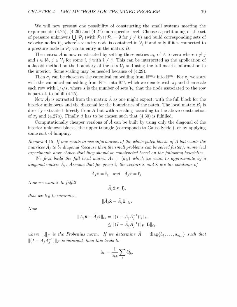
CHAPTER 4. AMG METHODS FOR THE MIXED PROBLEM 70
We will now present one possibility of constructing the small systems meeting therequirements (4.25), (4.26) and (4.27) on a specific level. Choose a partitioning of the setof pressure unknowns
⋃j Pj (with Pj ∩ Pk = ∅ for j 6= k) and build corresponding sets of
velocity nodes Vj, where a velocity node is contained in Vj if and only if it is connected toa pressure node in Pj via an entry in the matrix B.
The matrix A is now constructed by setting those entries aij of A to zero where i 6= jand i ∈ Vı, j ∈ V for some ı, with ı 6= . This can be interpreted as the application ofa Jacobi method on the boundary of the sets Vj and using the full matrix information inthe interior. Some scaling may be needed because of (4.29).
Then σj can be chosen as the canonical embedding from Rml,j into Rml. For πj we startwith the canonical embedding from Rnl,j into Rnl, which we denote with πj and then scaleeach row with 1/
√s, where s is the number of sets Vk that the node associated to the row
is part of, to fulfill (4.25).Now Aj is extracted from the matrix A as one might expect, with the full block for the
interior unknowns and the diagonal for the boundaries of the patch. The local matrix Bj isdirectly extracted directly from B but with a scaling according to the above constructionof πj and (4.27b). Finally β has to be chosen such that (4.30) is fulfilled.
Computationally cheaper versions of A can be built by using only the diagonal of theinterior-unknown-blocks, the upper triangle (corresponds to Gauss-Seidel), or by applyingsome sort of lumping.
Remark 4.15. If one wants to use information of the whole patch blocks of A but wants thematrices Aj to be diagonal (because then the small problems can be solved faster), numericalexperiments have shown that they should be constructed based on the following heuristics.
We first build the full local matrix Aj = (akl) which we want to approximate by a
diagonal matrix Aj. Assume that for given fj the vectors x and x are the solutions of
Ajx = fj and Ajx = fj.
Now we want x to fulfillAjx ≈ fj,
thus we try to minimize‖Ajx− Ajx‖`2.
Now
‖Ajx− Ajx‖`2 = ‖(I − AjA−1j )fj‖`2
≤ ‖(I − AjA−1j )‖F‖fj‖`2 ,
where ‖.‖F is the Frobenius norm. If we determine A = diaga1, . . . , anl,j such that
‖(I − AjA−1j )‖F is minimal, then this leads to
ak =1
akk
∑
l
a2lk.
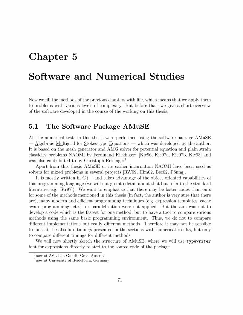
Chapter 5
Software and Numerical Studies
Now we fill the methods of the previous chapters with life, which means that we apply themto problems with various levels of complexity. But before that, we give a short overviewof the software developed in the course of the working on this thesis.
5.1 The Software Package AMuSE
All the numerical tests in this thesis were performed using the software package AMuSE— Algebraic Multigrid for Stokes-type Equations — which was developed by the author.It is based on the mesh generator and AMG solver for potential equation and plain strainelasticity problems NAOMI by Ferdinand Kickinger1 [Kic96, Kic97a, Kic97b, Kic98] andwas also contributed to by Christoph Reisinger2.
Apart from this thesis AMuSE or its earlier incarnation NAOMI have been used assolvers for mixed problems in several projects [RW99, Him02, Bec02, Ponng].
It is mostly written in C++ and takes advantage of the object oriented capabilities ofthis programming language (we will not go into detail about that but refer to the standardliterature, e.g. [Str97]). We want to emphasize that there may be faster codes than oursfor some of the methods mentioned in this thesis (in fact, the author is very sure that thereare), many modern and efficient programming techniques (e.g. expression templates, cacheaware programming, etc.) or parallelization were not applied. But the aim was not todevelop a code which is the fastest for one method, but to have a tool to compare variousmethods using the same basic programming environment. Thus, we do not to comparedifferent implementations but really different methods. Therefore it may not be sensibleto look at the absolute timings presented in the sections with numerical results, but onlyto compare different timings for different methods.
We will now shortly sketch the structure of AMuSE, where we will use typewriter
font for expressions directly related to the source code of the package.
1now at AVL List GmbH, Graz, Austria2now at University of Heidelberg, Germany
71
CHAPTER 5. SOFTWARE AND NUMERICAL STUDIES 72
Figure 5.1 The general structure of AMuSE. More complex dependencies (e.g. due tomoving meshes, etc.) were omitted in this figure.
PSfrag replacements
MeshHandler FEMGeneration
TimeStepper
NavierStokesSolver
BlockSystemSolver
method of lines + ODE
linearization
AMG solver for(A BT
B −C
)
5.1.1 Structure
The structure of the program is sketched in Figure 5.1. The central part (at least concerningthis thesis) is the block-system solver, its components are described in Figure 5.2.
The following external libraries and packages are used in parts of the program:
• Template Numerical Toolkit (TNT), Mathematical and Computational Sciences Divi-sion, National Institute of Standards and Technology, Gaithersburg, MD USA. Usedfor the direct solution of the coarse level systems.
• General Mesh Viewer (gmv), Applied Physics Division, Los Alamos National Labo-ratory, CA USA. Used for the visualization of the numerical results.
Figure 5.2 The block-system-solvers are implemented as derived classes of the baseAMuSE BlockSolver. Each one (except the direct solvers) can use a preconditioner, i.e.an object which is derived from AMuSE BlockPrecond. And the preconditioners (which usesome AMG solver) can use and manipulate the structures needed for an AMG method.
AMuSE BlockSolver
• Richardson,• GMRES,• BiCGstab,• SIMPLE,• direct,. . .
AMuSE BlockPrecond
• CoupledAMG,• “Black-Box”
(sec.2.5.3.1)
AMG ‘tools’• AMuSE GridTransfer
• AMuSE BlockSmoother
• AMuSE EllipticSmoother
CHAPTER 5. SOFTWARE AND NUMERICAL STUDIES 73
• gzstream, Deepak Bandyopadhay and Lutz Kettner, and zlib, Jean-Loup Gailly andMark Adler. Used for the compressed output of solutions.
• Linuxthreads, Xavier Leroy. Used for the shared memory parallelization of the FEMmatrix generation.
5.1.2 Matrices
AMuSE provides several sparse matrix classes which are substantial for the componentsdescribed above. As some non-standard ideas are used for their construction, we will sketchthem in this section.
The basic (templated) class is AMuSE SparseMatrixData< T >, where elements of typeT are stored in a similar way as compressed row storage (CRS) format, the only differenceis, that we use separate arrays for the element and index data of each single row, not onelong array for all elements. The template parameter T could be a scalar type like float
or double or again a small matrix (class AMuSE SmallMatrix< T, m, n >, where T is thetype of the entries and m and n are the row and column dimensions). This is used to storeblock matrices like
A1,1 A1,2 · · · A1,j
A2,1 A2,2 · · · A2,j
· · · · · · · · · · · ·Aj,1 Aj,2 · · · Aj,j
,
with k × k blocks Al,m (k j) with similar sparsity pattern, efficiently as
a1,1 a1,2 · · · a1,k
a2,1 a2,2 · · · a2,k
· · · · · · · · · · · ·ak,1 ak,2 · · · ak,k
,
with small j × j matrices al,m, where
(al,m)a,b = (Aa,b)l,m.
The AMuSE SparseMatrixData< T > class is only used for the storage of sparse matrices.The ‘mathematical’ objects (which can be multiplied with vectors, ‘inverted’, etc.) are oftype AMuSE SparseMatrix< T >.
The next generalization AMuSE MaskedSparseMatrix< T > can be understood in thefollowing way. Assume we want to store the matrix A of the Oseen linearized problem,which for example in 3D in general has the form
A
AA
. (5.1)
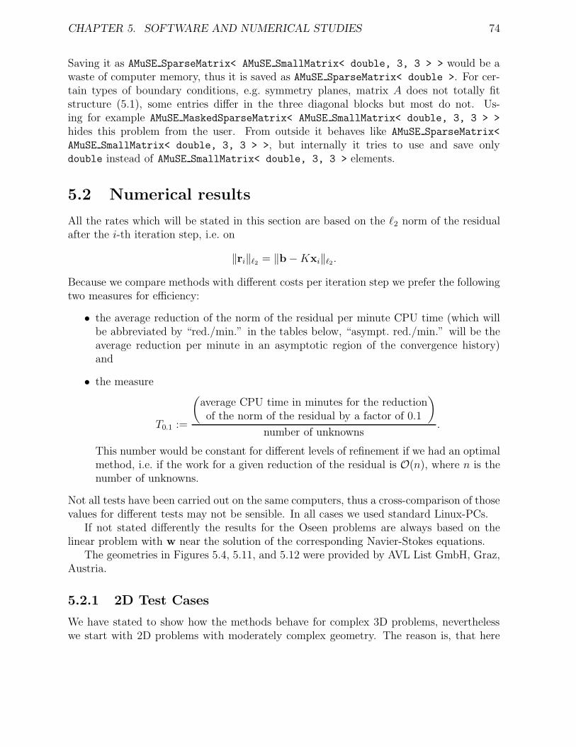
CHAPTER 5. SOFTWARE AND NUMERICAL STUDIES 74
Saving it as AMuSE SparseMatrix< AMuSE SmallMatrix< double, 3, 3 > > would be awaste of computer memory, thus it is saved as AMuSE SparseMatrix< double >. For cer-tain types of boundary conditions, e.g. symmetry planes, matrix A does not totally fitstructure (5.1), some entries differ in the three diagonal blocks but most do not. Us-ing for example AMuSE MaskedSparseMatrix< AMuSE SmallMatrix< double, 3, 3 > >
hides this problem from the user. From outside it behaves like AMuSE SparseMatrix<
AMuSE SmallMatrix< double, 3, 3 > >, but internally it tries to use and save onlydouble instead of AMuSE SmallMatrix< double, 3, 3 > elements.
5.2 Numerical results
All the rates which will be stated in this section are based on the `2 norm of the residualafter the i-th iteration step, i.e. on
‖ri‖`2 = ‖b−Kxi‖`2.
Because we compare methods with different costs per iteration step we prefer the followingtwo measures for efficiency:
• the average reduction of the norm of the residual per minute CPU time (which willbe abbreviated by “red./min.” in the tables below, “asympt. red./min.” will be theaverage reduction per minute in an asymptotic region of the convergence history)and
• the measure
T0.1 :=
(average CPU time in minutes for the reductionof the norm of the residual by a factor of 0.1
)
number of unknowns.
This number would be constant for different levels of refinement if we had an optimalmethod, i.e. if the work for a given reduction of the residual is O(n), where n is thenumber of unknowns.
Not all tests have been carried out on the same computers, thus a cross-comparison of thosevalues for different tests may not be sensible. In all cases we used standard Linux-PCs.
If not stated differently the results for the Oseen problems are always based on thelinear problem with w near the solution of the corresponding Navier-Stokes equations.
The geometries in Figures 5.4, 5.11, and 5.12 were provided by AVL List GmbH, Graz,Austria.
5.2.1 2D Test Cases
We have stated to show how the methods behave for complex 3D problems, neverthelesswe start with 2D problems with moderately complex geometry. The reason is, that here

CHAPTER 5. SOFTWARE AND NUMERICAL STUDIES 75
Figure 5.3 The initial mesh and the numerical solution of the driven cavity Stokes problem(lighter grey indicates higher velocities)
we can carry out parameter-studies for various methods on different levels in a reasonableperiod of time, which would not be possible otherwise.
Our two model problems are the following:
• Driven cavity. The initial grid (and the numerical solution of the Stokes problem)can be found in Figure 5.3. The problem is easily described, on a unit square we posea Dirichlet condition with velocity (1, 0) on the upper boundary and homogeneousDirichlet conditions on the rest of the boundary (the walls). The finer levels weregenerated by a hierarchical refinement of the coarse grid.
• 2D valve. Here the geometry is one half of the region round a valve with inlet-size0.03 and the distance between the walls at the narrowest part 0.003. The mesheswere generated using Ferdinand Kickinger’s NAOMI.
We pose two problems, one with symmetry boundary conditions along the symmetryplane, the other one with homogeneous Dirichlet conditions there. In both caseswe set Dirichlet condition with quadratic profile (with maximum velocity 1) on theupper boundary, natural outflow conditions on the lower boundary. The geometryand the solutions for the two problems (Navier-Stokes, ν = 5 · 10−4) are illustratedin Figure 5.4.
Dependence on Mesh Width
In the first set of tests we want to check the “h-independence” of the methods, i.e. we solvethe same Stokes problem on different levels of refinement and compare the efficiencies.We solve the driven cavity problem with modified Taylor-Hood-discretization and the red-black coloring algorithm with averaging for the coarse level construction. Just doing this
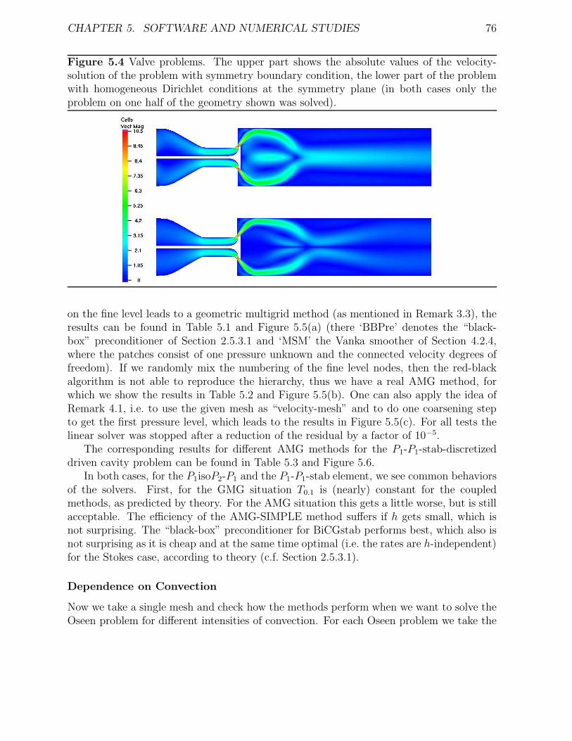
CHAPTER 5. SOFTWARE AND NUMERICAL STUDIES 76
Figure 5.4 Valve problems. The upper part shows the absolute values of the velocity-solution of the problem with symmetry boundary condition, the lower part of the problemwith homogeneous Dirichlet conditions at the symmetry plane (in both cases only theproblem on one half of the geometry shown was solved).
on the fine level leads to a geometric multigrid method (as mentioned in Remark 3.3), theresults can be found in Table 5.1 and Figure 5.5(a) (there ‘BBPre’ denotes the “black-box” preconditioner of Section 2.5.3.1 and ‘MSM’ the Vanka smoother of Section 4.2.4,where the patches consist of one pressure unknown and the connected velocity degrees offreedom). If we randomly mix the numbering of the fine level nodes, then the red-blackalgorithm is not able to reproduce the hierarchy, thus we have a real AMG method, forwhich we show the results in Table 5.2 and Figure 5.5(b). One can also apply the idea ofRemark 4.1, i.e. to use the given mesh as “velocity-mesh” and to do one coarsening stepto get the first pressure level, which leads to the results in Figure 5.5(c). For all tests thelinear solver was stopped after a reduction of the residual by a factor of 10−5.
The corresponding results for different AMG methods for the P1-P1-stab-discretizeddriven cavity problem can be found in Table 5.3 and Figure 5.6.
In both cases, for the P1isoP2-P1 and the P1-P1-stab element, we see common behaviorsof the solvers. First, for the GMG situation T0.1 is (nearly) constant for the coupledmethods, as predicted by theory. For the AMG situation this gets a little worse, but is stillacceptable. The efficiency of the AMG-SIMPLE method suffers if h gets small, which isnot surprising. The “black-box” preconditioner for BiCGstab performs best, which also isnot surprising as it is cheap and at the same time optimal (i.e. the rates are h-independent)for the Stokes case, according to theory (c.f. Section 2.5.3.1).
Dependence on Convection
Now we take a single mesh and check how the methods perform when we want to solve theOseen problem for different intensities of convection. For each Oseen problem we take the
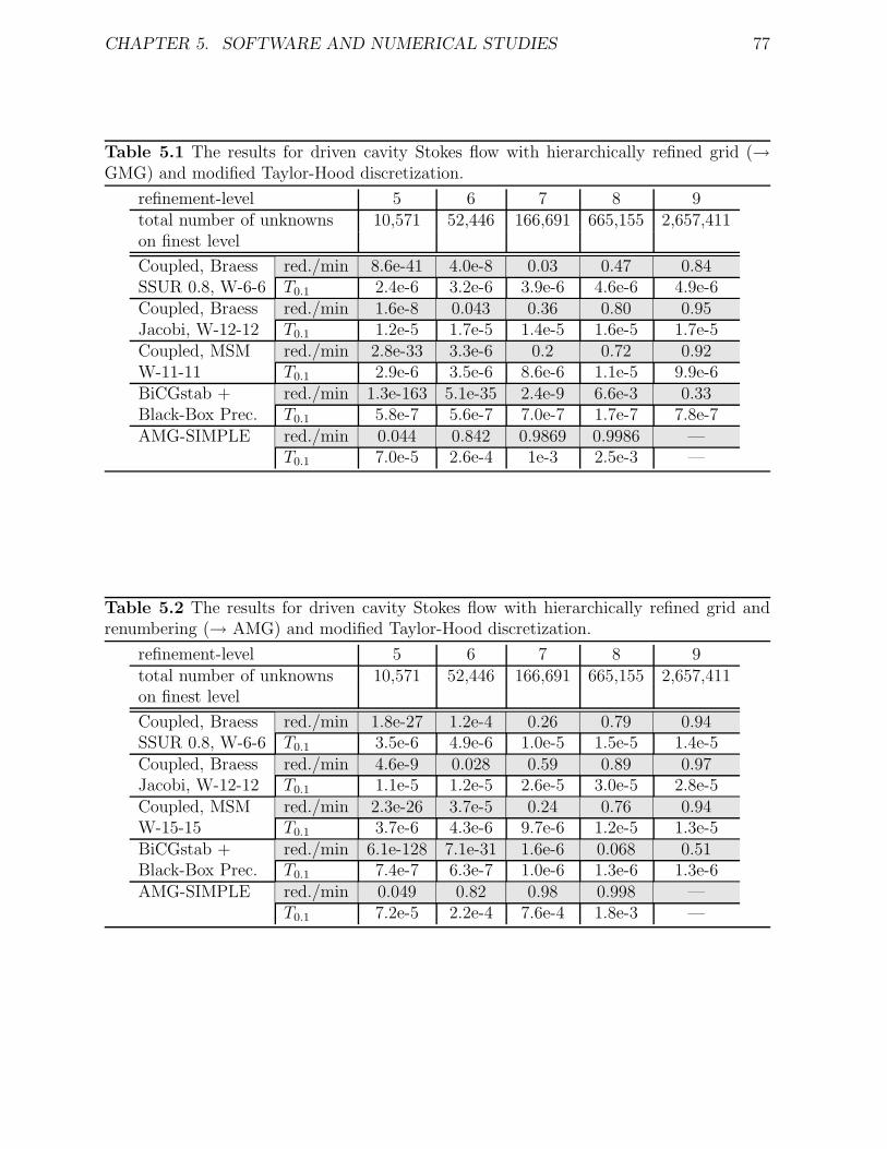
CHAPTER 5. SOFTWARE AND NUMERICAL STUDIES 77
Table 5.1 The results for driven cavity Stokes flow with hierarchically refined grid (→GMG) and modified Taylor-Hood discretization.
refinement-level 5 6 7 8 9total number of unknowns 10,571 52,446 166,691 665,155 2,657,411on finest level
Coupled, Braess red./min 8.6e-41 4.0e-8 0.03 0.47 0.84SSUR 0.8, W-6-6 T0.1 2.4e-6 3.2e-6 3.9e-6 4.6e-6 4.9e-6Coupled, Braess red./min 1.6e-8 0.043 0.36 0.80 0.95Jacobi, W-12-12 T0.1 1.2e-5 1.7e-5 1.4e-5 1.6e-5 1.7e-5Coupled, MSM red./min 2.8e-33 3.3e-6 0.2 0.72 0.92W-11-11 T0.1 2.9e-6 3.5e-6 8.6e-6 1.1e-5 9.9e-6BiCGstab + red./min 1.3e-163 5.1e-35 2.4e-9 6.6e-3 0.33Black-Box Prec. T0.1 5.8e-7 5.6e-7 7.0e-7 1.7e-7 7.8e-7AMG-SIMPLE red./min 0.044 0.842 0.9869 0.9986 —
T0.1 7.0e-5 2.6e-4 1e-3 2.5e-3 —
Table 5.2 The results for driven cavity Stokes flow with hierarchically refined grid andrenumbering (→ AMG) and modified Taylor-Hood discretization.
refinement-level 5 6 7 8 9total number of unknowns 10,571 52,446 166,691 665,155 2,657,411on finest level
Coupled, Braess red./min 1.8e-27 1.2e-4 0.26 0.79 0.94SSUR 0.8, W-6-6 T0.1 3.5e-6 4.9e-6 1.0e-5 1.5e-5 1.4e-5Coupled, Braess red./min 4.6e-9 0.028 0.59 0.89 0.97Jacobi, W-12-12 T0.1 1.1e-5 1.2e-5 2.6e-5 3.0e-5 2.8e-5Coupled, MSM red./min 2.3e-26 3.7e-5 0.24 0.76 0.94W-15-15 T0.1 3.7e-6 4.3e-6 9.7e-6 1.2e-5 1.3e-5BiCGstab + red./min 6.1e-128 7.1e-31 1.6e-6 0.068 0.51Black-Box Prec. T0.1 7.4e-7 6.3e-7 1.0e-6 1.3e-6 1.3e-6AMG-SIMPLE red./min 0.049 0.82 0.98 0.998 —
T0.1 7.2e-5 2.2e-4 7.6e-4 1.8e-3 —
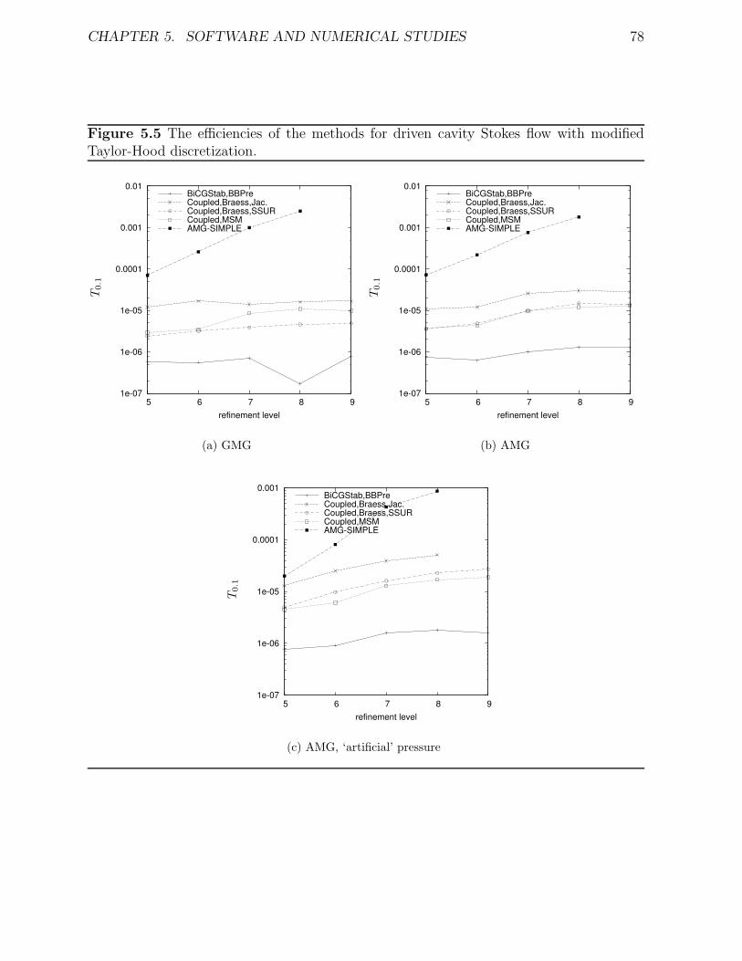
CHAPTER 5. SOFTWARE AND NUMERICAL STUDIES 78
Figure 5.5 The efficiencies of the methods for driven cavity Stokes flow with modifiedTaylor-Hood discretization.
1e-07
1e-06
1e-05
0.0001
0.001
0.01
5 6 7 8 9refinement level
BiCGStab,BBPreCoupled,Braess,Jac.Coupled,Braess,SSURCoupled,MSMAMG-SIMPLE
PSfrag replacements
T0.1
(a) GMG
1e-07
1e-06
1e-05
0.0001
0.001
0.01
5 6 7 8 9refinement level
BiCGStab,BBPreCoupled,Braess,Jac.Coupled,Braess,SSURCoupled,MSMAMG-SIMPLE
PSfrag replacements
T0.1
(b) AMG
1e-07
1e-06
1e-05
0.0001
0.001
5 6 7 8 9refinement level
BiCGStab,BBPreCoupled,Braess,Jac.Coupled,Braess,SSURCoupled,MSMAMG-SIMPLE
PSfrag replacements
T0.1
(c) AMG, ‘artificial’ pressure
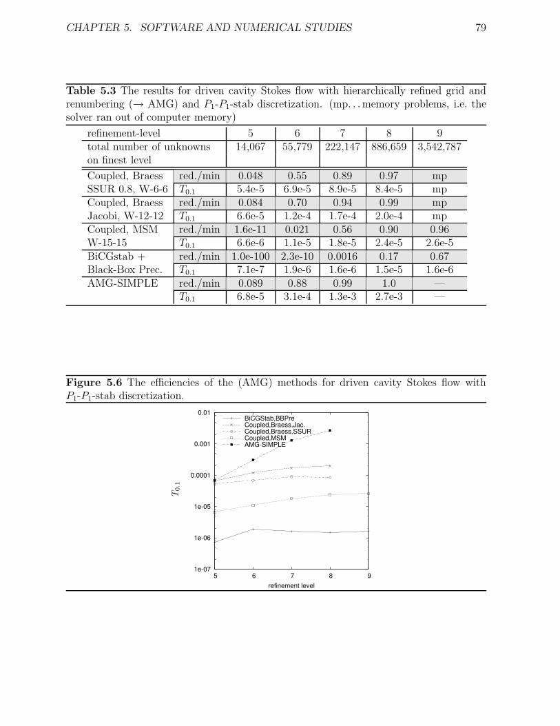
CHAPTER 5. SOFTWARE AND NUMERICAL STUDIES 79
Table 5.3 The results for driven cavity Stokes flow with hierarchically refined grid andrenumbering (→ AMG) and P1-P1-stab discretization. (mp. . . memory problems, i.e. thesolver ran out of computer memory)
refinement-level 5 6 7 8 9total number of unknowns 14,067 55,779 222,147 886,659 3,542,787on finest level
Coupled, Braess red./min 0.048 0.55 0.89 0.97 mpSSUR 0.8, W-6-6 T0.1 5.4e-5 6.9e-5 8.9e-5 8.4e-5 mpCoupled, Braess red./min 0.084 0.70 0.94 0.99 mpJacobi, W-12-12 T0.1 6.6e-5 1.2e-4 1.7e-4 2.0e-4 mpCoupled, MSM red./min 1.6e-11 0.021 0.56 0.90 0.96W-15-15 T0.1 6.6e-6 1.1e-5 1.8e-5 2.4e-5 2.6e-5BiCGstab + red./min 1.0e-100 2.3e-10 0.0016 0.17 0.67Black-Box Prec. T0.1 7.1e-7 1.9e-6 1.6e-6 1.5e-5 1.6e-6AMG-SIMPLE red./min 0.089 0.88 0.99 1.0 —
T0.1 6.8e-5 3.1e-4 1.3e-3 2.7e-3 —
Figure 5.6 The efficiencies of the (AMG) methods for driven cavity Stokes flow withP1-P1-stab discretization.
1e-07
1e-06
1e-05
0.0001
0.001
0.01
5 6 7 8 9refinement level
BiCGStab,BBPreCoupled,Braess,Jac.Coupled,Braess,SSURCoupled,MSMAMG-SIMPLE
PSfrag replacements
T0.1
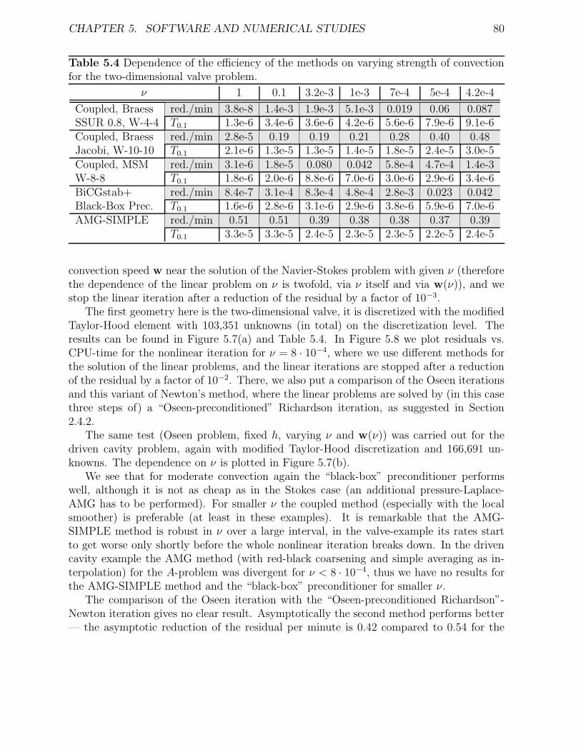
CHAPTER 5. SOFTWARE AND NUMERICAL STUDIES 80
Table 5.4 Dependence of the efficiency of the methods on varying strength of convectionfor the two-dimensional valve problem.
ν 1 0.1 3.2e-3 1e-3 7e-4 5e-4 4.2e-4
Coupled, Braess red./min 3.8e-8 1.4e-3 1.9e-3 5.1e-3 0.019 0.06 0.087SSUR 0.8, W-4-4 T0.1 1.3e-6 3.4e-6 3.6e-6 4.2e-6 5.6e-6 7.9e-6 9.1e-6Coupled, Braess red./min 2.8e-5 0.19 0.19 0.21 0.28 0.40 0.48Jacobi, W-10-10 T0.1 2.1e-6 1.3e-5 1.3e-5 1.4e-5 1.8e-5 2.4e-5 3.0e-5Coupled, MSM red./min 3.1e-6 1.8e-5 0.080 0.042 5.8e-4 4.7e-4 1.4e-3W-8-8 T0.1 1.8e-6 2.0e-6 8.8e-6 7.0e-6 3.0e-6 2.9e-6 3.4e-6BiCGstab+ red./min 8.4e-7 3.1e-4 8.3e-4 4.8e-4 2.8e-3 0.023 0.042Black-Box Prec. T0.1 1.6e-6 2.8e-6 3.1e-6 2.9e-6 3.8e-6 5.9e-6 7.0e-6AMG-SIMPLE red./min 0.51 0.51 0.39 0.38 0.38 0.37 0.39
T0.1 3.3e-5 3.3e-5 2.4e-5 2.3e-5 2.3e-5 2.2e-5 2.4e-5
convection speed w near the solution of the Navier-Stokes problem with given ν (thereforethe dependence of the linear problem on ν is twofold, via ν itself and via w(ν)), and westop the linear iteration after a reduction of the residual by a factor of 10−3.
The first geometry here is the two-dimensional valve, it is discretized with the modifiedTaylor-Hood element with 103,351 unknowns (in total) on the discretization level. Theresults can be found in Figure 5.7(a) and Table 5.4. In Figure 5.8 we plot residuals vs.CPU-time for the nonlinear iteration for ν = 8 · 10−4, where we use different methods forthe solution of the linear problems, and the linear iterations are stopped after a reductionof the residual by a factor of 10−2. There, we also put a comparison of the Oseen iterationsand this variant of Newton’s method, where the linear problems are solved by (in this casethree steps of) a “Oseen-preconditioned” Richardson iteration, as suggested in Section2.4.2.
The same test (Oseen problem, fixed h, varying ν and w(ν)) was carried out for thedriven cavity problem, again with modified Taylor-Hood discretization and 166,691 un-knowns. The dependence on ν is plotted in Figure 5.7(b).
We see that for moderate convection again the “black-box” preconditioner performswell, although it is not as cheap as in the Stokes case (an additional pressure-Laplace-AMG has to be performed). For smaller ν the coupled method (especially with the localsmoother) is preferable (at least in these examples). It is remarkable that the AMG-SIMPLE method is robust in ν over a large interval, in the valve-example its rates startto get worse only shortly before the whole nonlinear iteration breaks down. In the drivencavity example the AMG method (with red-black coarsening and simple averaging as in-terpolation) for the A-problem was divergent for ν < 8 · 10−4, thus we have no results forthe AMG-SIMPLE method and the “black-box” preconditioner for smaller ν.
The comparison of the Oseen iteration with the “Oseen-preconditioned Richardson”-Newton iteration gives no clear result. Asymptotically the second method performs better— the asymptotic reduction of the residual per minute is 0.42 compared to 0.54 for the
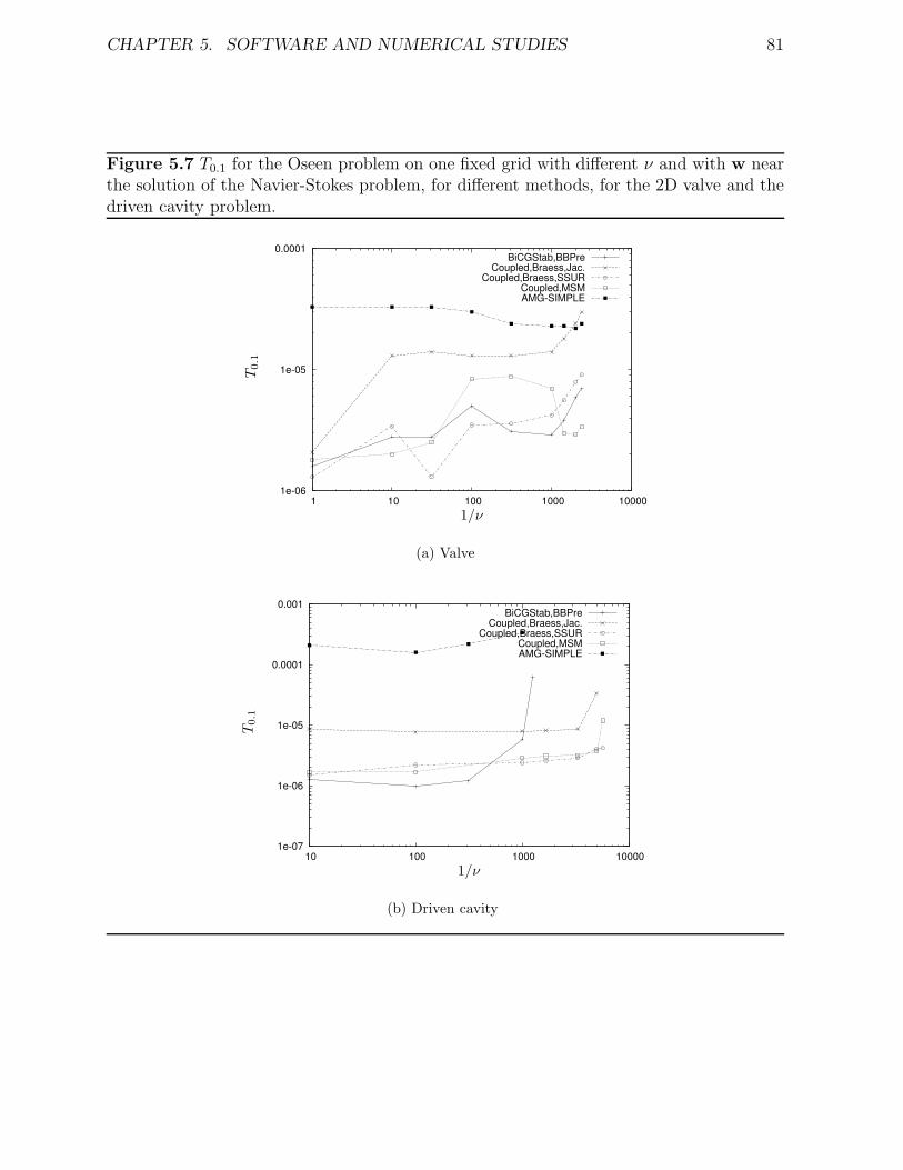
CHAPTER 5. SOFTWARE AND NUMERICAL STUDIES 81
Figure 5.7 T0.1 for the Oseen problem on one fixed grid with different ν and with w nearthe solution of the Navier-Stokes problem, for different methods, for the 2D valve and thedriven cavity problem.
1e-06
1e-05
0.0001
1 10 100 1000 10000
BiCGStab,BBPreCoupled,Braess,Jac.
Coupled,Braess,SSURCoupled,MSMAMG-SIMPLE
PSfrag replacements
1/ν
T0.1
(a) Valve
1e-07
1e-06
1e-05
0.0001
0.001
10 100 1000 10000
BiCGStab,BBPreCoupled,Braess,Jac.
Coupled,Braess,SSURCoupled,MSMAMG-SIMPLE
PSfrag replacements
1/ν
T0.1
(b) Driven cavity
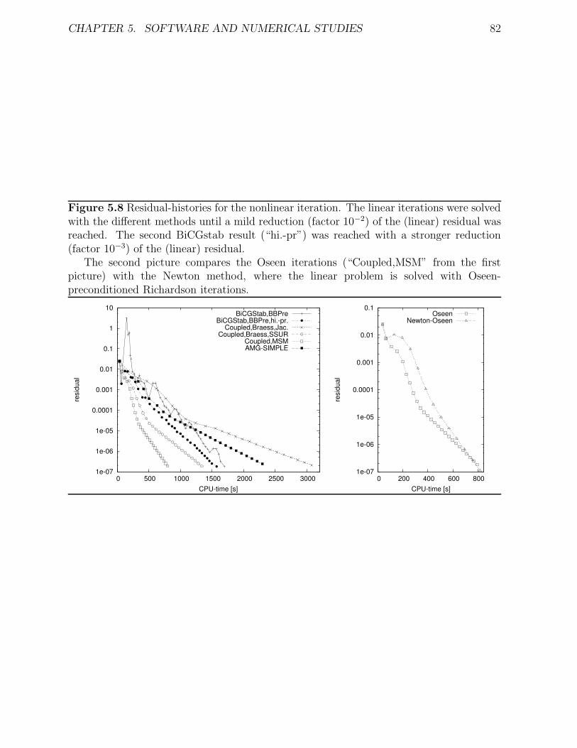
CHAPTER 5. SOFTWARE AND NUMERICAL STUDIES 82
Figure 5.8 Residual-histories for the nonlinear iteration. The linear iterations were solvedwith the different methods until a mild reduction (factor 10−2) of the (linear) residual wasreached. The second BiCGstab result (“hi.-pr”) was reached with a stronger reduction(factor 10−3) of the (linear) residual.proThe second picture compares the Oseen iterations (“Coupled,MSM” from the firstpicture) with the Newton method, where the linear problem is solved with Oseen-preconditioned Richardson iterations.
1e-07
1e-06
1e-05
0.0001
0.001
0.01
0.1
1
10
0 500 1000 1500 2000 2500 3000
resi
dual
CPU-time [s]
BiCGStab,BBPreBiCGStab,BBPre,hi.-pr.
Coupled,Braess,Jac.Coupled,Braess,SSUR
Coupled,MSMAMG-SIMPLE
1e-07
1e-06
1e-05
0.0001
0.001
0.01
0.1
0 200 400 600 800
resi
dual
CPU-time [s]
OseenNewton-Oseen
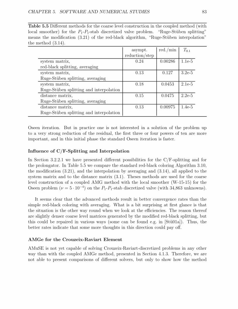
CHAPTER 5. SOFTWARE AND NUMERICAL STUDIES 83
Table 5.5 Different methods for the coarse level construction in the coupled method (withlocal smoother) for the P1-P1-stab discretized valve problem. “Ruge-Stuben splitting”means the modification (3.21) of the red-black algorithm, “Ruge-Stuben interpolation”the method (3.14).
asympt. red./min T0.1
reduction/stepsystem matrix, 0.24 0.00286 1.1e-5red-black splitting, averagingsystem matrix, 0.13 0.127 3.2e-5Ruge-Stuben splitting, averagingsystem matrix, 0.18 0.0453 2.1e-5Ruge-Stuben splitting and interpolationdistance matrix, 0.15 0.0475 2.2e-5Ruge-Stuben splitting, averagingdistance matrix, 0.13 0.00975 1.4e-5Ruge-Stuben splitting and interpolation
Oseen iteration. But in practice one is not interested in a solution of the problem upto a very strong reduction of the residual, the first three or four powers of ten are moreimportant, and in this initial phase the standard Oseen iteration is faster.
Influence of C/F-Splitting and Interpolation
In Section 3.2.2.1 we have presented different possibilities for the C/F-splitting and forthe prolongator. In Table 5.5 we compare the standard red-black coloring Algorithm 3.10,the modification (3.21), and the interpolation by averaging and (3.14), all applied to thesystem matrix and to the distance matrix (3.1). Theses methods are used for the coarselevel construction of a coupled AMG method with the local smoother (W-15-15) for theOseen problem (ν = 5 · 10−4) on the P1-P1-stab discretized valve (with 34,863 unknowns).
It seems clear that the advanced methods result in better convergence rates than thesimple red-black coloring with averaging. What is a bit surprising at first glance is thatthe situation is the other way round when we look at the efficiencies. The reason thereofare slightly denser coarse level matrices generated by the modified red-black splitting, butthis could be repaired in various ways (some can be found e.g. in [Stu01a]). Thus, thebetter rates indicate that some more thoughts in this direction could pay off.
AMGe for the Crouzeix-Raviart Element
AMuSE is not yet capable of solving Crouzeix-Raviart-discretized problems in any otherway than with the coupled AMGe method, presented in Section 4.1.3. Therefore, we arenot able to present comparisons of different solvers, but only to show how the method
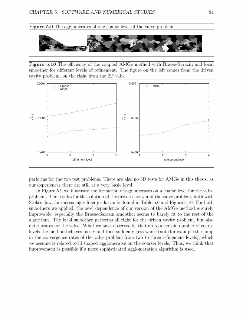
CHAPTER 5. SOFTWARE AND NUMERICAL STUDIES 84
Figure 5.9 The agglomerates of one coarse level of the valve problem.
Figure 5.10 The efficiency of the coupled AMGe method with Braess-Sarazin and localsmoother for different levels of refinement. The figure on the left comes from the drivencavity problem, on the right from the 2D valve.
1e-06
1e-05
0.0001
5 6 7 8refinement level
BraessMSM
PSfrag replacements
T0.1
1e-06
1e-05
0.0001
1 2 3 4refinement level
MSM
PSfrag replacements
T0.1
performs for the two test problems. There are also no 3D tests for AMGe in this thesis, asour experiences there are still at a very basic level.
In Figure 5.9 we illustrate the formation of agglomerates on a coarse level for the valveproblem. The results for the solution of the driven cavity and the valve problem, both withStokes flow, for increasingly finer grids can be found in Table 5.6 and Figure 5.10. For bothsmoothers we applied, the level dependence of our version of the AMGe method is surelyimprovable, especially the Braess-Sarazin smoother seems to barely fit to the rest of thealgorithm. The local smoother performs all right for the driven cavity problem, but alsodeteriorates for the valve. What we have observed is, that up to a certain number of coarselevels the method behaves nicely and then suddenly gets worse (note for example the jumpin the convergence rates of the valve problem from two to three refinement levels), whichwe assume is related to ill shaped agglomerates on the coarser levels. Thus, we think thatimprovement is possible if a more sophisticated agglomeration algorithm is used.
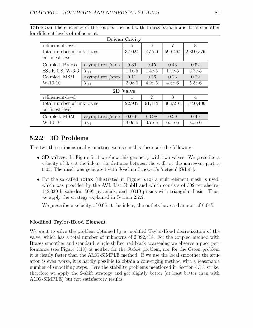
CHAPTER 5. SOFTWARE AND NUMERICAL STUDIES 85
Table 5.6 The efficiency of the coupled method with Braess-Sarazin and local smootherfor different levels of refinement.
Driven Cavityrefinement-level 5 6 7 8total number of unknowns 37,024 147,776 590,464 2,360,576on finest level
Coupled, Braess asympt.red./step 0.39 0.45 0.43 0.52SSUR 0.8, W-6-6 T0.1 1.1e-5 1.4e-5 1.9e-5 2.7e-5Coupled, MSM asympt.red./step 0.11 0.26 0.23 0.29W-10-10 T0.1 2.9e-6 4.2e-6 4.6e-6 5.3e-6
2D Valverefinement-level 1 2 3 4total number of unknowns 22,932 91,112 363,216 1,450,400on finest level
Coupled, MSM asympt.red./step 0.046 0.098 0.30 0.40W-10-10 T0.1 3.0e-6 3.7e-6 6.3e-6 8.5e-6
5.2.2 3D Problems
The two three-dimensional geometries we use in this thesis are the following:
• 3D valves. In Figure 5.11 we show this geometry with two valves. We prescribe avelocity of 0.5 at the inlets, the distance between the walls at the narrowest part is0.03. The mesh was generated with Joachim Schoberl’s ‘netgen’ [Sch97].
• For the so called rotax (illustrated in Figure 5.12) a multi-element mesh is used,which was provided by the AVL List GmbH and which consists of 302 tetrahedra,142,339 hexahedra, 5095 pyramids, and 10019 prisms with triangular basis. Thus,we apply the strategy explained in Section 2.2.2.
We prescribe a velocity of 0.05 at the inlets, the outlets have a diameter of 0.045.
Modified Taylor-Hood Element
We want to solve the problem obtained by a modified Taylor-Hood discretization of thevalve, which has a total number of unknowns of 2,092,418. For the coupled method withBraess smoother and standard, single-shifted red-black coarsening we observe a poor per-formance (see Figure 5.13) as neither for the Stokes problem, nor for the Oseen problemit is clearly faster than the AMG-SIMPLE method. If we use the local smoother the situ-ation is even worse, it is hardly possible to obtain a converging method with a reasonablenumber of smoothing steps. Here the stability problems mentioned in Section 4.1.1 strike,therefore we apply the 2-shift strategy and get slightly better (at least better than withAMG-SIMPLE) but not satisfactory results.
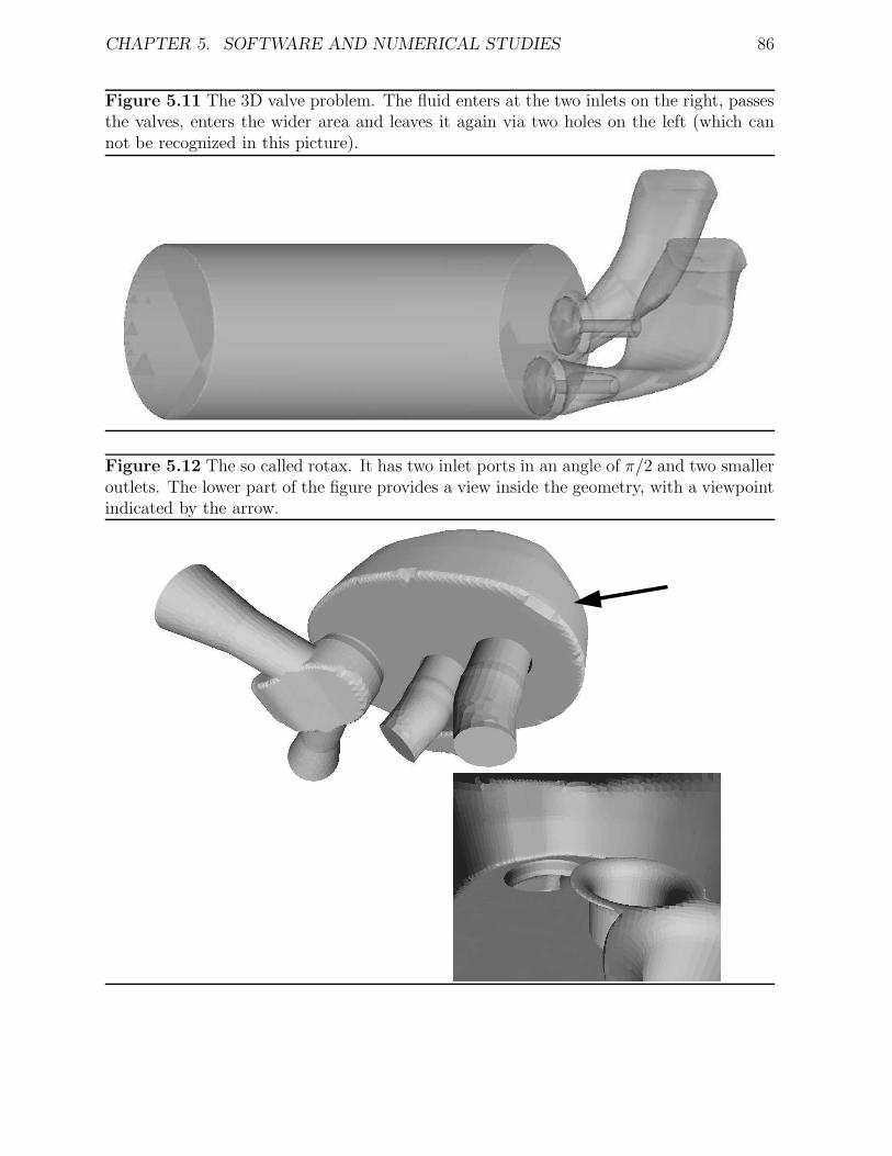
CHAPTER 5. SOFTWARE AND NUMERICAL STUDIES 86
Figure 5.11 The 3D valve problem. The fluid enters at the two inlets on the right, passesthe valves, enters the wider area and leaves it again via two holes on the left (which cannot be recognized in this picture).
Figure 5.12 The so called rotax. It has two inlet ports in an angle of π/2 and two smalleroutlets. The lower part of the figure provides a view inside the geometry, with a viewpointindicated by the arrow.
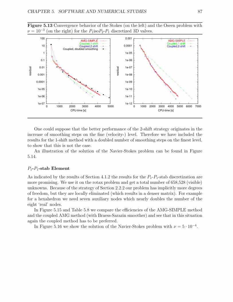
CHAPTER 5. SOFTWARE AND NUMERICAL STUDIES 87
Figure 5.13 Convergence behavior of the Stokes (on the left) and the Oseen problem withν = 10−3 (on the right) for the P1isoP2-P1 discretized 3D valves.
1e-07
1e-06
1e-05
0.0001
0.001
0.01
0.1
1
10
100
0 1000 2000 3000 4000 5000
resi
dual
CPU-time [s]
AMG-SIMPLECoupled,1-shiftCoupled,2-shift
Coupled, doubled smoothing
1e-12
1e-11
1e-10
1e-09
1e-08
1e-07
1e-06
1e-05
0.0001
0.001
0 1000 2000 3000 4000 5000 6000 7000
resi
dual
CPU-time [s]
AMG-SIMPLECoupled,1-shiftCoupled,2-shift
One could suppose that the better performance of the 2-shift strategy originates in theincrease of smoothing steps on the fine (velocity-) level. Therefore we have included theresults for the 1-shift method with a doubled number of smoothing steps on the finest level,to show that this is not the case.
An illustration of the solution of the Navier-Stokes problem can be found in Figure5.14.
P1-P1-stab Element
As indicated by the results of Section 4.1.2 the results for the P1-P1-stab discretization aremore promising. We use it on the rotax problem and get a total number of 658,528 (visible)unknowns. Because of the strategy of Section 2.2.2 our problem has implicitly more degreesof freedom, but they are locally eliminated (which results in a denser matrix). For examplefor a hexahedron we need seven auxiliary nodes which nearly doubles the number of theeight ‘real’ nodes.
In Figure 5.15 and Table 5.8 we compare the efficiencies of the AMG-SIMPLE methodand the coupled AMG method (with Braess-Sarazin smoother) and see that in this situationagain the coupled method has to be preferred.
In Figure 5.16 we show the solution of the Navier-Stokes problem with ν = 5 · 10−4.
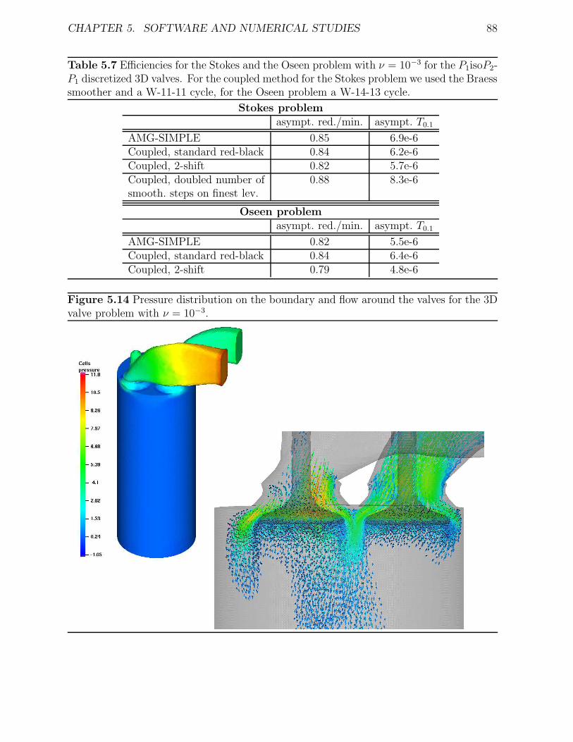
CHAPTER 5. SOFTWARE AND NUMERICAL STUDIES 88
Table 5.7 Efficiencies for the Stokes and the Oseen problem with ν = 10−3 for the P1isoP2-P1 discretized 3D valves. For the coupled method for the Stokes problem we used the Braesssmoother and a W-11-11 cycle, for the Oseen problem a W-14-13 cycle.
Stokes problemasympt. red./min. asympt. T0.1
AMG-SIMPLE 0.85 6.9e-6Coupled, standard red-black 0.84 6.2e-6Coupled, 2-shift 0.82 5.7e-6Coupled, doubled number of 0.88 8.3e-6smooth. steps on finest lev.
Oseen problemasympt. red./min. asympt. T0.1
AMG-SIMPLE 0.82 5.5e-6Coupled, standard red-black 0.84 6.4e-6Coupled, 2-shift 0.79 4.8e-6
Figure 5.14 Pressure distribution on the boundary and flow around the valves for the 3Dvalve problem with ν = 10−3.
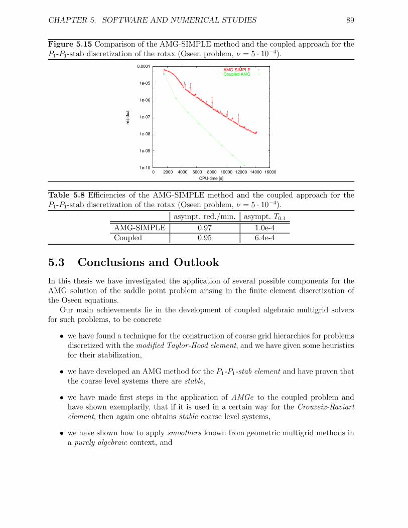
CHAPTER 5. SOFTWARE AND NUMERICAL STUDIES 89
Figure 5.15 Comparison of the AMG-SIMPLE method and the coupled approach for theP1-P1-stab discretization of the rotax (Oseen problem, ν = 5 · 10−4).
1e-10
1e-09
1e-08
1e-07
1e-06
1e-05
0.0001
0 2000 4000 6000 8000 10000 12000 14000 16000
resi
dual
CPU-time [s]
AMG-SIMPLECoupled AMG
Table 5.8 Efficiencies of the AMG-SIMPLE method and the coupled approach for theP1-P1-stab discretization of the rotax (Oseen problem, ν = 5 · 10−4).
asympt. red./min. asympt. T0.1
AMG-SIMPLE 0.97 1.0e-4Coupled 0.95 6.4e-4
5.3 Conclusions and Outlook
In this thesis we have investigated the application of several possible components for theAMG solution of the saddle point problem arising in the finite element discretization ofthe Oseen equations.
Our main achievements lie in the development of coupled algebraic multigrid solversfor such problems, to be concrete
• we have found a technique for the construction of coarse grid hierarchies for problemsdiscretized with the modified Taylor-Hood element, and we have given some heuristicsfor their stabilization,
• we have developed an AMG method for the P1-P1-stab element and have proven thatthe coarse level systems there are stable,
• we have made first steps in the application of AMGe to the coupled problem andhave shown exemplarily, that if it is used in a certain way for the Crouzeix-Raviartelement, then again one obtains stable coarse level systems,
• we have shown how to apply smoothers known from geometric multigrid methods ina purely algebraic context, and
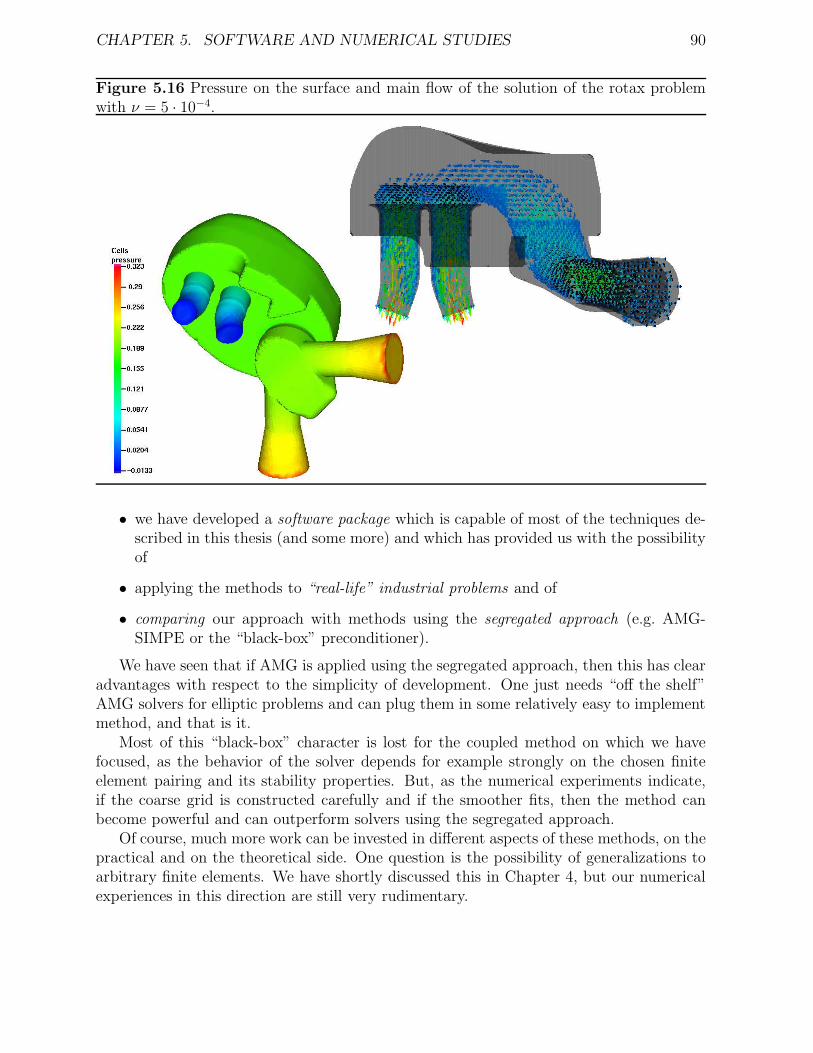
CHAPTER 5. SOFTWARE AND NUMERICAL STUDIES 90
Figure 5.16 Pressure on the surface and main flow of the solution of the rotax problemwith ν = 5 · 10−4.
• we have developed a software package which is capable of most of the techniques de-scribed in this thesis (and some more) and which has provided us with the possibilityof
• applying the methods to “real-life” industrial problems and of
• comparing our approach with methods using the segregated approach (e.g. AMG-SIMPE or the “black-box” preconditioner).
We have seen that if AMG is applied using the segregated approach, then this has clearadvantages with respect to the simplicity of development. One just needs “off the shelf”AMG solvers for elliptic problems and can plug them in some relatively easy to implementmethod, and that is it.
Most of this “black-box” character is lost for the coupled method on which we havefocused, as the behavior of the solver depends for example strongly on the chosen finiteelement pairing and its stability properties. But, as the numerical experiments indicate,if the coarse grid is constructed carefully and if the smoother fits, then the method canbecome powerful and can outperform solvers using the segregated approach.
Of course, much more work can be invested in different aspects of these methods, on thepractical and on the theoretical side. One question is the possibility of generalizations toarbitrary finite elements. We have shortly discussed this in Chapter 4, but our numericalexperiences in this direction are still very rudimentary.
CHAPTER 5. SOFTWARE AND NUMERICAL STUDIES 91
Other questions arise on the analytic side. We have proven (in some cases) the stabilityof the coarse level system, but what about convergence? What about stability results fora more general class of elements?
If the methods presented here should be used in an industrial context, then some morethought should also be spent on an efficient implementation, on modern programmingtechniques, on parallelization aspects, etc.
Nevertheless, we have developed a coupled method which can compete with classicalapproaches, and which has an area of application beyond unit square problems with weakconvection.
Bibliography
[AB01] V.A.O. Anjorin and I.E. Barton. Removal of temporal and under-relaxationterms from the pressure-correction equation of the SIMPLE algorithm. Int.J. Fluid Dynamics, 5:59–75, 2001.
[Ada03] M.F. Adams. Algebraic multrigrid methods for constrained linear systemswith applications to contact problems in solid mechanics. preprint availableat http://www.cs.berkeley.edu/∼madams/, 2003. submitted to NumericalLinear Algebra with Applications.
[AHU58] K. Arrow, L. Hurwicz, and H. Uzawa. Studies in nonlinear programming.Stanford University Press, Stanford, CA, 1958.
[Ast71] G.P. Astrachancev. An iterative method for solving elliptic net problems.USSR Comput. Math. Math. Phys., 11(2):171–182, 1971.
[BA72] I. Babuska and A.K. Aziz. Survey lectures on the mathematical foundationsof the finite element method. With the collaboration of G. Fix and R.B.Kellogg. In A.K. Aziz, editor, The Mathematical Foundation of the FiniteElement Method with Applications to Partial Differential Equations, Sympos.Univ. Maryland, Baltimore 1972, pages 3–363. Academic Press, New York -London, 1972.
[Bac66] N.S. Bachvalov. On the convergence of a relaxation methods with natu-ral constraints on the elliptic operator. USSR Comput. Math. Math. Phys.,6(5):101–135, 1966.
[BCF+00] M. Brezina, A.J. Cleary, R.D. Falgout, V.E. Henson, J.E. Jones, T.A. Man-teufel, S.F. McCormick, and J.W. Ruge. Algebraic multigrid based on elementinterpolation (AMGe). SIAM J. Sci. Comput., 22(5):1570–1592, 2000.
[Bec95] R. Becker. An adaptive finite element method for the incompressible Navier-Stokes equations on time-dependent domains. Preprint 95-44, SFB 359, Uni-versity Heidelberg, 1995.
[Bec02] A. Becirovic. Berechnung von Gebietsableitungen fur das Stokes-Problem.Master’s thesis, Johannes Kepler University Linz, 2002.
92
BIBLIOGRAPHY 93
[Ber02] S. Bertling. Ein Algebraisches Mehrgitterverfahren zur Losung der Stokes-Gleichungen. Master’s thesis, RWTH Aachen, 2002.
[BF91] F. Brezzi and M. Fortin. Mixed and Hybrid Finite Element Methods. Springerseries in computational mathematics. Springer, New York, 1991.
[BMR84] A. Brandt, S. McCormick, and J. Ruge. Algebraic multigrid (AMG) for sparsematrix equations. In D.J. Evans, editor, Sparsity and its applications, pages257–284. Cambridge University Press, Cambridge, 1984.
[Bra73] A. Brandt. Multi-level adaptive techniques (mlat) for fast numerical solu-tion to boundary value problems. In Proc. 3rd Internat. Conf. on NumericalMethods in Fluid Mechanics, held in Paris, 1972, Lecture Notes in Physics,1973.
[Bra77] A. Brandt. Multi-level adaptive solutions to boundary-value problems. Math.Comput., 31:333–390, 1977.
[Bra86] A. Brandt. Algebraic multigrid theory: The symmetric case. Appl. Math.Comp., 19:23–56, 1986.
[Bra93] J.H. Bramble. Multigrid methods. Longman Scientific & Technical, Harlow,1993.
[Bra97] D. Braess. Finite Elemente. Springer, Berlin, Heidelberg, New York, 2ndedition, 1997.
[Bre93] S.C. Brenner. A nonconforming mixed multigrid method for the pure displace-ment problem in planar linear elasticity. SIAM J. Numer. Anal., 30(1):116–135, 1993.
[BS97] D. Braess and R. Sarazin. An efficient smoother for the Stokes problem. Appl.Numer. Math., 23:3–20, 1997.
[Bun88] H. Bungartz. Algebraische Mehrgitterverfahren zur Optimierung unterNebenbedingungen. Master’s thesis, TU Munich, 1988.
[BV90] D. Braess and R. Verfurth. Multigrid methods for nonconforming finite ele-ment methods. SIAM J. Numer. Anal., 27(4):979–986, 1990.
[BW97] J. Bey and G. Wittum. Downwind numbering: Robust multigrid forconvection-diffusion problems. Appl. Numer. Math., 23(1):177–192, 1997.
[BWY90] R.E. Bank, B.D. Welfert, and H. Yserentant. A class of iterative methods forsolving saddle point problems. Num. Math., 56:645–666, 1990.
BIBLIOGRAPHY 94
[CR73] M. Crouzeix and P.A. Raviart. Conforming and nonconforming finite elementmethods for solving the stationary Stokes equations I. RAIRO Anal. Numer.,7:33–76, 1973.
[Dic00] D. Dickson. Mathematicians chase the seven million-dollar proofs. Nature,405:383, 25 May 2000.
[DMS01] W. Dahmen, S. Muller, and T. Schlinkmann. On an adaptive multigrid solverfor convection-dominated problems. SIAM J. Sci. Comput., 23(3):781–804,2001.
[ESW02] H.C. Elman, D.J. Silvester, and A.J. Wathen. Performance and analysisof saddle point preconditioners for the discrete steady-state Navier-Stokesequations. Numer. Math., 90:665–688, 2002.
[Fed61] R.P. Federenko. A relaxation method for elliptic difference equations. USSRComput. Math. Math. Phys., 1(5):1092–1069, 1961.
[Fef00] C.L. Fefferman. Existence & smoothness of the Navier-Stokes equation. avail-able at http://www.claymath.org, 2000. Official problem description of the”Millenium Price Problem”.
[Fei93] M. Feistauer. Mathematical Methods in Fluid Dynamics. Number 67 in Pit-man Monographs and Surveys in Pure and Applied Mathematics. LongmanScientific & Technical, London, 1993.
[FHS93] L.P. Franca, T.J.R. Hughes, and R. Stenberg. Stabilized finite element meth-ods for the Stokes problem. In M. Gunzburger and R.A. Nicolaides, edi-tors, Incompressible Computational Fluid Dynamics, chapter 4, pages 87–107.Cambridge University Press, 1993.
[FM93] L.P. Franca and A.L. Madureira. Element diameter free stability parametersfor stabilized methods applied to fluids. Comp. Meth. Appl. Mech. Eng.,105:395–403, 1993.
[FS91] L.P. Franca and R. Stenberg. Error analysis of some Galerkin least squaresmethods for the elasticity equations. SIAM J. Numer. Anal., 28(6):1680–1697,1991.
[GNR98] M. Griebel, T. Neunhoeffer, and H. Regler. Algebraic multigrid methods forthe solution of the Navier-Stokes equations in complicated geometries. Int. J.Numer. Methods Fluids, 26:281–301, 1998.
[GR86] V. Girault and P.A. Raviart. Finite Element Methods for Navier-Stokes Equa-tions. Springer, Berlin, Heidelberg, 1986.
BIBLIOGRAPHY 95
[Hac76] W. Hackbusch. Implementation of the multi-grid method for solving partialdifferential equations. Technical report RA 82, IBM T.J. Watson ResearchCenter, 1976.
[Hac85] W. Hackbusch. Multi-Grid Methods and Applications. Springer, Berlin, 1985.
[Hac93] W. Hackbusch. Iterative Losung großer schwachbesetzter Gleichungssysteme.Teubner, Stuttgart, 2nd edition, 1993.
[Him02] J. Himmelbauer. Numerische Losung der Navier-Stokes-Gleichung bei zeit-abhangiger Geometrie. Master’s thesis, Johannes Kepler University Linz,2002.
[HV01] V.E. Henson and P.S. Vassilevski. Element-free AMGe: General algo-rithms for computing interpolation weights in AMG. SIAM J. Sci. Comput.,23(2):629–650, 2001.
[HW02] E. Hairer and G. Wanner. Solving Ordinary Differential Equations II, Stiffand Differential-Algebraic Problems. Springer, Heidelberg, 2nd, rev. edition,2002.
[HWN00] E. Hairer, G. Wanner, and S.P. Nørsett. Solving Ordinary Differential Equa-tions I, Nonstiff Problems. Springer, Heidelberg, 2nd, rev. edition, 2000.
[Ips01] I.C.F. Ipsen. A note on preconditioning nonsymmetric matrices. SIAM J.Sci. Comput., 23(3):1050–1051, 2001.
[IRT93] J. Iliash, T. Rossi, and J. Toivanen. Two iterative methods for solving theStokes problem. Report 2/1993, Department of Mathematics, University ofJyvaskyla, 1993.
[JKMT02] V. John, P. Knobloch, G. Matthies, and L. Tobiska. Non-nested multi-level solvers for finite element discretizations of mixed problems. Computing,68:313–341, 2002.
[JV01] J.E. Jones and P.S. Vassilevski. AMGe based on element agglomeration.SIAM J. Sci. Comput., 23(1):109–133, 2001.
[JVW02] J.E. Jones, P.S. Vassilevski, and C.S. Woodward. Nonlinear Schwarz-FASmethods for unstructured finite element problems. Technical Report UCRL-JC-150427, Lawrence Livermore National Laboratory, 2002. submitted to theSecond M.I.T. Conference on Computational Fluid and Solid Mechanics, heldin Cambridge, MA, June 17–20, 2003.
[Kic96] F. Kickinger. Algebraic multigrid for discrete elliptic second-order problems— a program description. Technical Report No. 96-5, Department of Mathe-matics, Johannes Kepler University, Linz, 1996.
BIBLIOGRAPHY 96
[Kic97a] F. Kickinger. Automatic microscaling mesh generation. Institusbericht No.525, Department of Mathematics, Johannes Kepler University, Linz, 1997.
[Kic97b] F. Kickinger. Programmbeschreibung NAOMI 2D und Algebraic Multigrid.Technical Report No. 97-4, Department of Mathematics, Johannes KeplerUniversity, Linz, 1997.
[Kic98] F. Kickinger. Algebraic multigrid for discrete elliptic second-order problems.In W. Hackbusch, G. Wittum, and R. Nieminen, editors, Multigrid MethodsV, Proceedings of the 5th European Multigrid conference, held in Stuttgart,Germany, 1996, volume 3 of Lect. Notes Comput. Sci. Eng., pages 157–172,Berlin, 1998. Springer.
[Kor77] V.G. Korneev. Finite element schemes of higher order of accuracy (in Rus-sian). Leningrad University Press, Leningrad, 1977.
[Lan82] U. Langer. On the choice of iterative parameters in the relaxation methodon a sequence of meshes. USSR Comput. Math. Math. Phys., 22(5):98–114,1982.
[LQ86] U. Langer and W. Queck. On the convergence factor of Uzawa’s algorithm.J. Comput. Appl. Math., 15:191–202, 1986.
[LQ87] U. Langer and W. Queck. Preconditioned Uzawa-type iterative methodsfor solving mixed finite element equations. Wissenschaftliche Schriftenreiheder Technischen Universitat Karl-Marx-Stadt, Karl-Marx-Stadt (Chemnitz),1987.
[LW02] D. Loghin and A.J. Wathen. Schur complement preconditioning for ellipticsystems of partial differential equations. Technical Report 01/20, OxfordUniversity Computing Laboratory, Numerical Analysis Group, 2002.
[Meu99] G. Meurant. Computer solution of large linear systems, volume 28 of Studiesin Mathematics and its Applications. Elsevier, Amsterdam, 1999.
[MGW00] M.F. Murphy, G.H. Golub, and A.J. Wathen. A note on preconditioning forindefinite linear systems. SIAM J. Sci. Comput., 21(6):1969–1972, 2000.
[MP94] B. Mohammadi and O. Pironneau. Analysis of the K-Epsilon TURBULENCEMODEL. John Wiley & Sons, Chichester, 1994.
[OGWW98] C.W. Oosterlee, F.J. Gaspar, T. Washio, and R. Wienands. Fast multigridsolvers for higher order upwind discretizations of convection-dominated prob-lems. In W. Hackbusch, G. Wittum, and R. Nieminen, editors, Multigridmethods V. Proceedings of the 5th European multigrid conference, held inStuttgart, Germany, 1996, volume 3 of Lect. Notes Comput. Sci. Eng., pages212–224, Berlin, 1998. Springer.
BIBLIOGRAPHY 97
[Pat80] S. Patankar. Numerical heat transfer and fluid flow. Series in ComputationalMethods in Mechanics and Thermal Sciences. McGraw-Hill, New York, 1980.
[Pir89] O. Pironneau. Finite Element Methods for Fluids. John Wiley & Sons, Chich-ester, 1989.
[Ponng] A. Ponitz. Shape optimization for the Navier-Stokes equations. Master’sthesis, Johannes Kepler University Linz, ongoing.
[PS72] S. Patankar and D. Spalding. A calculation procedure for heat, mass andmomentum transfer in three-dimensional parabolic flows. Int. J. Heat MassTransfer, 15:1787–1806, 1972.
[PTV00] S.I. Petrova, L. Tobiska, and P.S. Vassilevski. Multigrid methods based onmatrix-dependent coarse spaces for nonconforming streamline-diffusion finiteelement discretization of convection-diffusion problems. East-West J. Numer.Math., 8(3):223–242, 2000.
[Ran00] R. Rannacher. Finite Element Methods for the Incompressible Navier-StokesEquations. In Giovanni Galdi et al., editors, Fundamental directions in math-ematical fluid mechanics, pages 191–293. Birkhauser, Basel, 2000.
[Raw95] M.J. Raw. A coupled algebraic multigrid method for the 3D Navier-Stokesequations. In W. Hackbusch and G. Wittum, editors, Fast solvers for flowproblems. Proceedings of the tenth GAMM-Seminar, held in Kiel, Germany,1994, volume 49 of Notes Numer. Fluid Mech., pages 204–215, Wiesbaden,1995. Vieweg.
[Rei01] S. Reitzinger. Algebraic Multigrid Methods for Large Scale Finite ElementEquations. PhD thesis, Johannes Kepler University, Linz, 2001.
[Reu95] A. Reusken. A new robust multigrid method for 2D convection diffusionproblems. In W. Hackbusch and G. Wittum, editors, Fast solvers for flowproblems. Proceedings of the tenth GAMM-Seminar, held in Kiel, Germany,1994, volume 49 of Notes Numer. Fluid Mech., pages 229–240, Wiesbaden,1995. Vieweg.
[Reu02] A. Reusken. Convergence analysis of a multigrid method for convection-diffusion equations. Numer. Math., 91(2):323–349, 2002.
[RS86] J.W. Ruge and K. Stuben. Algebraic multigrid (AMG). In S. McCormick,editor, Multigrid Methods, volume 5 of Frontiers in Applied Mathematics,pages 73–130. SIAM, 1986.
[RW92] T. Rusten and R. Winther. A preconditioned iterative method for saddlepointproblems. SIAM J. Matrix Anal. Appl., 13(3):887–904, 1992.
BIBLIOGRAPHY 98
[RW99] C. Reisinger and M. Wabro. Analysis and numerical solution of the k-ε tur-bulence model with non-standard boundary conditions. Master’s thesis, Jo-hannes Kepler University Linz, 1999.
[Sch97] J. Schoberl. Netgen — an advancing front 2D/3D-mesh generator basedon abstract rules. Comput. Visual. Sci., 1:41–52, 1997. Netgen homepage:www.hpfem.jku.at/netgen/.
[SEKW01] D. Silvester, H. Elman, D. Kay, and A. Wathen. Efficient preconditioningof the linearized Navier-Stokes equations for incompressible flow. Journal ofComputational and Applied Mathematics, 128:261–279, 2001.
[SS86] Y. Saad and M.H. Schultz. GMRES: A generalized minimal residual algorithmfor solving nonsymmetric linear systems. SIAM J. Sci. Stat. Comput., 7:856–869, 1986.
[Str97] B. Stroustrup. The C++ Programming Language. Addison-Wesley, Boston,3rd edition, 1997.
[Stu01a] K. Stuben. An introduction to algebraic multigrid. In U. Trottenberg,C. Oosterlee, and A. Schuller, editors, Multigrid, pages 413–532. AcademicPress, New York - London, 2001.
[Stu01b] K. Stuben. A review of algebraic multigrid. Computational and AppliedMathematics, 128:281–309, 2001.
[SVdV94] G.L.G. Sleijpen and H.A. Van der Vorst. Maintaining convergence propertiesof BiCGstab methods in finite precision arithmetic. Preprint 861, Departmentof Mathematics, University Utrecht, 1994.
[SW94] D.J. Silvester and A.J. Wathen. Fast iterative solution of stabilised Stokes sys-tems. II. Using general block preconditioners. SIAM J. Num. Anal., 31:1352–1367, 1994.
[SZ03] J. Schoberl and W. Zulehner. On Schwarz-type smoothers for saddle pointproblems. Numer. Math., 95(2):377–399, 2003.
[TOS01] U. Trottenberg, C. Oosterlee, and A. Schuller. Multigrid. Academic Press,New York - London, 2001.
[Tur99] S. Turek. Efficient Solvers for Incompressible Flow Problems. Lecture Notesin Computational Science and Engineering. Springer, Heidelberg, 1999.
[Van86] S. Vanka. Block-implicit multigrid calculation of two-dimensional recirculat-ing flows. Comp. Meth. Appl. Mech. Eng., 59(1):29–48, 1986.
BIBLIOGRAPHY 99
[VdV92] H.A. Van der Vorst. Bi-CGstab: A fast and smoothly converging variant ofBi-CG for the solution of nonsymmetric linear systems. SIAM J. Sci. Stat.Comput., 13(2):631–644, 1992.
[Ver84a] R. Verfurth. Error estimates for a mixed finite element approximation of theStokes equations. R.A.I.R.O. Num. Anal., 18(2):175–182, 1984.
[Ver84b] R. Verfurth. A multilevel algorithm for mixed problems. SIAM J. Numer.Anal., 21:264–271, 1984.
[Vos93] H. Voss. Iterative methods for linear systems of equations. Textbook of the3rd International Summerschool Jyvaskyla, Finland. Hamburger Beitrage zurAngewandten Mathematik, Reihe B: Berichte, Hamburg, 1993.
[Web94] R. Webster. An algebraic multigrid solver for Navier-Stokes problems. Int. J.Numer. Meth. Fluids, 18:761–780, 1994.
[Wes92] P. Wesseling. An introduction to multigrid methods. John Wiley & Sons Ltd.,Chichester, 1992.
[Wit89] G. Wittum. Multi-grid methods for Stokes and Navier-Stokes equations. Nu-mer. Math., 54:543–563, 1989.
[Wit90] G. Wittum. On the convergence of multi-grid methods with transformingsmoothers. Numer. Math., 57:15–38, 1990.
[Yos80] K. Yosida. Functional analysis. Springer, Berlin-Heidelberg-New York, 6thedition, 1980.
[YVB98] I. Yavneh, C.H. Venner, and A. Brandt. Fast multigrid solution of the advec-tion problem with closed characteristics. SIAM J. Sci. Comput., 19(1):111–125, 1998.
[Zul00] W. Zulehner. A class of smoothers for saddle point problems. Computing,65(3):227–246, 2000.
[Zul02] W. Zulehner. Analysis of iterative methods for saddle point problems: aunified approach. Mathematics of Computation, 71(238):479–505, 2002.

Index
A-stable, 23strongly, 23
agglomeration, see element agglomerationAMG-SIMPLE, 30AMGe, 45AMuSE, 71
external libraries, 72matrices, 73structure, 72
approximation property, 38, 39Arrow-Hurwicz algorithm, 31auxiliary matrix, 35
BiCGstab, 28black box preconditioner, 33Braess-Sarazin smoother, see smoother
C/F-splitting, 40coarse grid correction, 37condition number, 31convective term
instability, 24nonlinearity, 25
Crank-Nicolson scheme, 23Crouzeix-Raviart element, 21
direct neighborhood, 42discretization parameter, 18
element agglomeration, 47red-grey-black, 47
essentially positive type, 41Euler scheme
explicit, 23implicit, 23
FE-AMG-isomorphism, 49
FE-isomorphism, 18finite element method, 16fractional-step-θ-scheme, 23
Galerkin projection, 36geometric multigrid methods, 37–39GMRES, 27
inf-sup condition, 15, 16, 52, 53inner condensation, 21
Krylov space methods, 27–29
L-stable, 23Laplacian, 18LBB condition, 15, 16, 53, see inf-sup con-
dition
M-matrix, 41mass matrix, 18multi-element meshes, 21
Navier-Stokes equations, 12
one-step-θ scheme, 23Oseen equations, 13
P1isoP2-P1 element, 19, 51P nc
1 -P0 element, 21, 58P1-P1 element
stabilized, 20, 53unstabilized, 17
P2-P1 element, 19polar set, 15pressure mass matrix, 18prolongation matrix, 35
red-black-coloring method, 44
100
INDEX 101
restriction matrix, 36
segregated approach, 48SIMPLE, 29, 64smoother
Braess-Sarazin, 65squared system, 64transforming, 64Vanka, 68
smoothing operator, 36smoothing property, 38, 39smoothing rate, 38stability function, 23Stokes equations, 13streamline upwinding Petrov Galerkin scheme,
25strongly negatively coupled, 44
transposed, 44
T0.1, 74Taylor-Hood element, 19
modified, 19transforming smoother, see smoothertwo-grid operator, 38
Uzawa methodclassical, 31inexact, 31inexact symmetric, 31, 65
Vanka smoother, see smoother
weak formulation, 14
Lebenslauf
Dipl.-Ing. Markus WabroAm Nordsaum 29A-4050 Traun
Geboren: 24.11.1975 in Linz, OsterreichEltern: Hermann Wabro, Adelheid Puchner, geborene SchabetsbergerBruder: Michael WabroVerheiratet mit Karolin Wabro, geborene Hagenbuchner
Ausbildung
1982 – 1986: Besuch der Volksschule 18 in Linz.1986 – 1994: Besuch des Bundesrealgymnasiums Linz, Landwiedstraße.06.1994: Ablegung der Matura mit Auszeichnung.1994–1999: Studium der Technischen Mathematik an der Johannes Kepler Uni-
versitat in Linz.06.1999: Ablegung der Diplomprufung mit Auszeichnung.
Berufliche Laufbahn
1994 – 1999: Abhaltung diverser Kurse in Mathematik bzw. EDV an der Volks-hochschule, dem Wirtschaftsforderungsinsitut, dem Arbeitsmarkt-service und dem Studienkreis.
07.1999 – 05.2000: Mitarbeiter an der J.K. Universitat in Linz, an der Abteilung furNumerische Mathematik und Optimierung, im FFF-Projekt “Auto-matischer Multi-Element Netzgenerator und StromungssimulatorAUTOGEN”.
06.2000 – 05.2001: Zivildienst beim Roten Kreuz in Traun.06.2001 – 09.2001: Mitarbeiter an der J.K. Universitat in Linz, am Institut fur Nu-
merische Mathematik. Arbeit an einem Industrieprojekt in Ko-operation mit der AVL List GmbH, Graz.
seit 10.2001: Mitarbeiter an der J.K. Universitat, Institut fur Numerische Mathe-matik. Arbeit am FWF-Projekt “Robust Algebraic Multigrid Meth-ods and their Parallelization”.
102