introduction to multiple regression - statpowerstatpower.net/content/312/lecture...
TRANSCRIPT

Introduction to Multiple Regression
James H. Steiger
Department of Psychology and Human DevelopmentVanderbilt University
James H. Steiger (Vanderbilt University) 1 / 54

Introduction to Multiple Regression1 The Multiple Regression Model
2 Some Key Regression Terminology
3 The Kids Data Example
Visualizing the Data – The Scatterplot Matrix
Regression Models for Predicting Weight
4 Understanding Regression Coefficients
5 Statistical Testing in the Fixed Regressor Model
Introduction
Partial F -Tests: A General Approach
Partial F -Tests: Overall Regression
Partial F -Tests: Adding a Single Term
6 Variable Selection in Multiple Regression
Introduction
Forward Selection
Backward Elimination
Stepwise Regression
Automatic Single-Term Sequential Testing in R
7 Variable Selection in R
Problems with Statistical Testing in the Variable Selection Context
8 Information-Based Selection Criteria
The Active Terms
Information Criteria
9 (Estimated)Standard Errors
10 Standard Errors for Predicted and Fitted Values
James H. Steiger (Vanderbilt University) 2 / 54
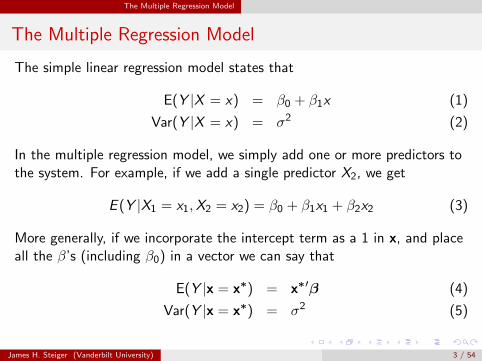
The Multiple Regression Model
The Multiple Regression Model
The simple linear regression model states that
E(Y |X = x) = β0 + β1x (1)
Var(Y |X = x) = σ2 (2)
In the multiple regression model, we simply add one or more predictors tothe system. For example, if we add a single predictor X2, we get
E (Y |X1 = x1,X2 = x2) = β0 + β1x1 + β2x2 (3)
More generally, if we incorporate the intercept term as a 1 in x, and placeall the β’s (including β0) in a vector we can say that
E(Y |x = x∗) = x∗′β (4)
Var(Y |x = x∗) = σ2 (5)
James H. Steiger (Vanderbilt University) 3 / 54
The Multiple Regression Model
Challenges in Multiple Regression
Dealing with multiple predictors is considerably more challenging thandealing with only a single predictor. Some of the problems include:
Choosing the best model. In multiple regression, often severaldifferent sets of variables perform equally well in predicting acriterion. Which set should you use?
Interactions between variables. In some cases, independent variablesinteract, and the regression equation will not be accurate unless thisinteraction is taken into account.
James H. Steiger (Vanderbilt University) 4 / 54

The Multiple Regression Model
Challenges in Multiple Regression
Much greater difficulty visualizing the regression relationships. Withonly one independent variable, the regression line can be plottedneatly in two dimensions. With two predictors, there is a regressionsurface instead of a regression line, and with 3 predictors and onecriterion, you run out of dimensions for plotting.
Model interpretation becomes substantially more difficult. Themultiple regression equation changes as each new variable is added tothe model. Since the regression weights for each variable are modifiedby the other variables, and hence depend on what is in the model, thesubstantive interpretation of the regression equation is problematic.
James H. Steiger (Vanderbilt University) 5 / 54

Some Key Regression Terminology
Some Key Regression TerminologyIntroduction
In Section 3.3 of ALR, Weisberg introduces a number of key ideas andnomenclature in connection with a regression model of the form
E (Y |X ) = β0 + β1X1 + · · ·+ βpXp (6)
James H. Steiger (Vanderbilt University) 6 / 54

Some Key Regression Terminology
Some Key Regression TerminologyPredictors vs. Terms
Regression problems start with a collection of potential predictors.
Some of these may be continuous measurements, like the height orweight of an object.
Some may be discrete but ordered, like a doctor’s rating of overallhealth of a patient on a nine-point scale.
Other potential predictors can be categorical, like eye color or anindicator of whether a particular unit received a treatment.
All these types of potential predictors can be useful in multiple linearregression.
A key notion is the distinction between predictors and terms in theregression equation.
In early discussions, these are often synonymous. However, we quicklylearn that they need not be.
James H. Steiger (Vanderbilt University) 7 / 54

Some Key Regression Terminology
Some Key Regression TerminologyTypes of Terms
Many types of terms can be created from a group of predictors. Here aresome examples
The intercept. We can rewrite the mean function on the previousslide as
E (Y |X ) = β0X0 + β1X1 + · · ·+ βpXp (7)
where X0 is a term that is always equal to one. Mean functionswithout an intercept would not have this term included.
Predictors. The simplest type of term is simply one of the predictors.
James H. Steiger (Vanderbilt University) 8 / 54
Some Key Regression Terminology
Some Key Regression TerminologyTypes of Terms
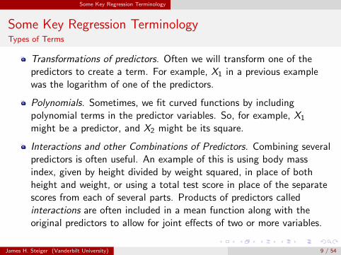
Transformations of predictors. Often we will transform one of thepredictors to create a term. For example, X1 in a previous examplewas the logarithm of one of the predictors.
Polynomials. Sometimes, we fit curved functions by includingpolynomial terms in the predictor variables. So, for example, X1
might be a predictor, and X2 might be its square.
Interactions and other Combinations of Predictors. Combining severalpredictors is often useful. An example of this is using body massindex, given by height divided by weight squared, in place of bothheight and weight, or using a total test score in place of the separatescores from each of several parts. Products of predictors calledinteractions are often included in a mean function along with theoriginal predictors to allow for joint effects of two or more variables.
James H. Steiger (Vanderbilt University) 9 / 54

Some Key Regression Terminology
Some Key Regression TerminologyTypes of Terms
Dummy Variables and Factors. A categorical predictor with two ormore levels is called a factor. Factors are included in multiple linearregression using dummy variables, which are typically terms that haveonly two values, often zero and one, indicating which category ispresent for a particular observation. We will see in ALR, Chapter 6that a categorical predictor with two categories can be represented byone dummy variable, while a categorical predictor with manycategories can require several dummy variables.
Comment. A regression with k predictors may contain fewer than k termsor more than k terms.
James H. Steiger (Vanderbilt University) 10 / 54

The Kids Data Example
Kids Data
Example (The Kids Data)
As an example consider the following data from the Kleinbaum, Kupperand Miller text on regression analysis. These data show weight, height,and age of a random sample of 12 nutritionally deficient children. Thedata are available online in the file KidsDataR.txt.
James H. Steiger (Vanderbilt University) 11 / 54

The Kids Data Example
Kids Data
WGT(y) HGT(x1) AGE(x2)
64 57 871 59 1053 49 667 62 1155 51 858 50 777 55 1057 48 956 42 1051 42 676 61 1268 57 9
James H. Steiger (Vanderbilt University) 12 / 54

The Kids Data Example Visualizing the Data – The Scatterplot Matrix
The Scatterplot Matrix
The scatterplot matrix on the next slide shows that both HGT and AGE
are strongly linearly related to WGT. However, the two potentialpredictors are also strongly linearly related to each other.
This is corroborated by the correlation matrix for the three variables.
> kids.data <- read.table("KidsDataR.txt", header = T, sep = ",")
> cor(kids.data)
WGT HGT AGE
WGT 1.0000 0.8143 0.7698
HGT 0.8143 1.0000 0.6138
AGE 0.7698 0.6138 1.0000
James H. Steiger (Vanderbilt University) 13 / 54

The Kids Data Example Visualizing the Data – The Scatterplot Matrix
The Scatterplot Matrix> pairs(kids.data)
WGT
45 50 55 60
5055
6065
7075
4550
5560
HGT
50 55 60 65 70 75 6 7 8 9 10 11 12
67
89
1011
12
AGE
James H. Steiger (Vanderbilt University) 14 / 54

The Kids Data Example Regression Models for Predicting Weight
Potential Regression Models
The situation here is relatively simple.
We can see that height is the best predictor of weight.
Age is also an excellent predictor, but because it is also correlatedwith height, it may not add too much to the prediction equation.
We fit the two models in succession. The first model has only heightas a predictor, while the second adds age.
In the following slides, we’ll perform the standard linear modelanalysis, and discuss the results, after which we’ll comment briefly onthe theory underlying the methods.
> attach(kids.data)
> model.1 <- lm(WGT ~ HGT)
> model.2 <- lm(WGT ~ HGT + AGE)
> summary(model.1)
> summary(model.2)
James H. Steiger (Vanderbilt University) 15 / 54
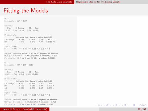
The Kids Data Example Regression Models for Predicting Weight
Fitting the ModelsCall:
lm(formula = WGT ~ HGT)
Residuals:
Min 1Q Median 3Q Max
-5.87 -3.90 -0.44 2.26 11.84
Coefficients:
Estimate Std. Error t value Pr(>|t|)
(Intercept) 6.190 12.849 0.48 0.6404
HGT 1.072 0.242 4.44 0.0013 **
---
Signif. codes:
0 '***' 0.001 '**' 0.01 '*' 0.05 '.' 0.1 ' ' 1
Residual standard error: 5.47 on 10 degrees of freedom
Multiple R-squared: 0.663,Adjusted R-squared: 0.629
F-statistic: 19.7 on 1 and 10 DF, p-value: 0.00126
Call:
lm(formula = WGT ~ HGT + AGE)
Residuals:
Min 1Q Median 3Q Max
-6.871 -1.700 0.345 1.464 10.234
Coefficients:
Estimate Std. Error t value Pr(>|t|)
(Intercept) 6.553 10.945 0.60 0.564
HGT 0.722 0.261 2.77 0.022 *
AGE 2.050 0.937 2.19 0.056 .
---
Signif. codes:
0 '***' 0.001 '**' 0.01 '*' 0.05 '.' 0.1 ' ' 1
Residual standard error: 4.66 on 9 degrees of freedom
Multiple R-squared: 0.78,Adjusted R-squared: 0.731
F-statistic: 16 on 2 and 9 DF, p-value: 0.0011
James H. Steiger (Vanderbilt University) 16 / 54
The Kids Data Example Regression Models for Predicting Weight
Comparing the Models with ANOVA
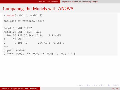
> anova(model.1, model.2)
Analysis of Variance Table
Model 1: WGT ~ HGT
Model 2: WGT ~ HGT + AGE
Res.Df RSS Df Sum of Sq F Pr(>F)
1 10 299
2 9 195 1 104 4.78 0.056 .
---
Signif. codes:
0 '***' 0.001 '**' 0.01 '*' 0.05 '.' 0.1 ' ' 1
James H. Steiger (Vanderbilt University) 17 / 54

The Kids Data Example Regression Models for Predicting Weight
The Squared Multiple Correlation Coefficient R2
The correlation between the predicted scores and the criterion scoresis called the multiple correlation coefficient,and is almost universallydenoted with the value R.
Curiously, many writers use this notation whether a sample or apopulation value is referred to, which creates some problems for somereaders.
We can eliminate this ambiguity by using either ρ2 or R2pop to signify
the population value.
Since R is always positive, and R2 is the percentage of variance in yaccounted for by the predictors (in the colloquial sense), mostdiscussions center on R2 rather than R.
When it is necessary for clarity, one can denote the squared multiplecorrelation as R2
y |x1x2to indicate that variates x1 and x2 have been
included in the regression equation.
James H. Steiger (Vanderbilt University) 18 / 54

The Kids Data Example Regression Models for Predicting Weight
The Partial Correlation Coefficient
The partial correlation coefficient is a measure of the strength of thelinear relationship between two variables after the contribution ofother variables has been “partialled out” or “controlled for” usinglinear regression.
We will use the notation ryx |w1,w2,...wpto stand for the partial
correlation between y and x with the w ’s partialled out.
This correlation is simply the Pearson correlation between theregression residual εy |w1,w2,...wp
for y with the w ’s as predictors andthe regression residual εx |w1,w2,...wp
of x with the w ’s as predictors.
James H. Steiger (Vanderbilt University) 19 / 54

The Kids Data Example Regression Models for Predicting Weight
Partial Regression Coefficients
In a similar approach to calculating partial correlation coefficients, wecan also calculate partial regression coefficients.
For example, the partial regression between y and xj with the otherx ’s partialled out is simply the slope of the regression line forpredicting the residual of y with the other x ’s partialled out from thatof xj with the other x ’s partialled out.
James H. Steiger (Vanderbilt University) 20 / 54

The Kids Data Example Regression Models for Predicting Weight
Bias of the Sample R2
When a population correlation is zero, the sample correlation is hardlyever zero. As a consequence, the R2 value obtained in an analysis ofsample data is a biased estimate of the population value.
An unbiased estimator is available (Olkin and Pratt, 1958), butrequires very powerful software like Mathematica to compute, andconsequently is not available in standard statistics packages. As aresult, these packages compute an approximate “shrunken” (or“adjusted”) estimate and report it alongside the uncorrected value.The adusted estimator when there are k predictors is
R2 = 1− (1− R2)N − 1
N − k − 1(8)
James H. Steiger (Vanderbilt University) 21 / 54
Understanding Regression Coefficients
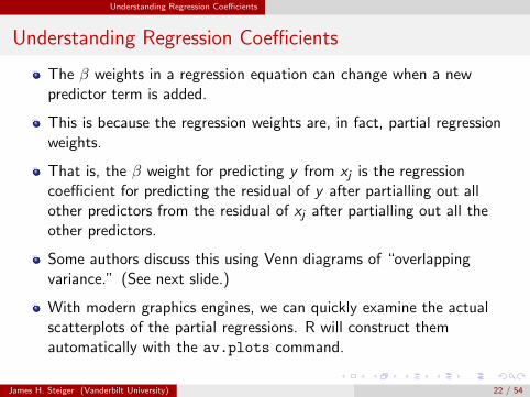
Understanding Regression Coefficients
The β weights in a regression equation can change when a newpredictor term is added.
This is because the regression weights are, in fact, partial regressionweights.
That is, the β weight for predicting y from xj is the regressioncoefficient for predicting the residual of y after partialling out allother predictors from the residual of xj after partialling out all theother predictors.
Some authors discuss this using Venn diagrams of “overlappingvariance.” (See next slide.)
With modern graphics engines, we can quickly examine the actualscatterplots of the partial regressions. R will construct themautomatically with the av.plots command.
James H. Steiger (Vanderbilt University) 22 / 54

Understanding Regression Coefficients
Venn Diagrams
James H. Steiger (Vanderbilt University) 23 / 54

Understanding Regression Coefficients
Added Variable Plots> library(car)
> av.plots(model.2)
Warning: ’av.plots’ is deprecated.
Use ’avPlots’ instead.
See help("Deprecated") and help("car-deprecated").
−10 −5 0 5
−10
−5
05
10
HGT | others
WG
T |
oth
ers
−2 −1 0 1 2 3
−5
05
10
AGE | others
WG
T |
oth
ers
Added−Variable Plots
James H. Steiger (Vanderbilt University) 24 / 54
Statistical Testing in the Fixed Regressor Model Introduction
Introduction
In connection with regression models, we’ve seen two different F tests.
One is the test of significance for the overall regression. This tests thenull hypothesis that, for the current model, R2 = 0 in the population.
The other test we frequently see is a model comparison F , whichtests the hypothesis that the R2 for the more complex model (whichhas all the terms of the previous model and some additional ones) isstatistically significantly larger than the R2 for the less complexmodel.
James H. Steiger (Vanderbilt University) 25 / 54

Statistical Testing in the Fixed Regressor Model Partial F -Tests: A General Approach
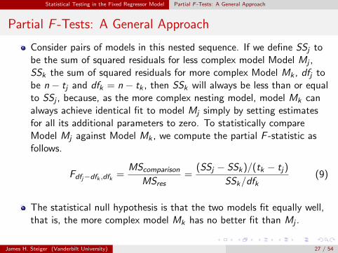
Partial F -Tests: A General Approach
Actually, the F -tests we’ve seen are a special case of a generalprocedure for generating partial F-tests on a nested sequence ofmodels.
Consider a sequence of J models Mj , j = 1, . . . , J. Suppose ModelMk includes Model Mj as a special case for all pairs of values ofj < k ≤ J. That is, Model Mj is a special case of Model Mk wheresome terms have coefficients of zero. Then Model Mj is nested withinModel Mk for all these values, and we say the set of models is anested sequence.
Define tj and tk respectively as the number of terms including theintercept term in models Mj and Mk .
As a mnemonic device, associate k with complex , because model Mk
is more complex (has more terms) than model Mj .
James H. Steiger (Vanderbilt University) 26 / 54
Statistical Testing in the Fixed Regressor Model Partial F -Tests: A General Approach
Partial F -Tests: A General Approach
Consider pairs of models in this nested sequence. If we define SSj tobe the sum of squared residuals for less complex model Model Mj ,SSk the sum of squared residuals for more complex Model Mk , dfj tobe n − tj and dfk = n − tk , then SSk will always be less than or equalto SSj , because, as the more complex nesting model, model Mk canalways achieve identical fit to model Mj simply by setting estimatesfor all its additional parameters to zero. To statistically compareModel Mj against Model Mk , we compute the partial F -statistic asfollows.
Fdfj−dfk ,dfk =MScomparison
MSres=
(SSj − SSk)/(tk − tj)
SSk/dfk(9)
The statistical null hypothesis is that the two models fit equally well,that is, the more complex model Mk has no better fit than Mj .
James H. Steiger (Vanderbilt University) 27 / 54

Statistical Testing in the Fixed Regressor Model Partial F -Tests: Overall Regression
Partial F -Tests: Overall Regression
The overall F test in linear regression is routinely reported inregression output when testing a model with one or more predictorterms in addition to an intercept. It tests the hypothesis thatR2pop = 0, against the alternative that R2
pop > 0.
The overall F test is simply a partial F test comparing a regressionmodel Mk with tk terms (including an intercept) with a model M1
that has only one intercept term.
Now, a model that has only an intercept term must, in least squaresregression, define the intercept coefficient β0 to be y , the mean of they scores, because it is well known that the sample mean is that valuearound which the sum of squared deviations is a minimum.
So SSj for the model with only an intercept term becomes SSy , thesum of squared deviations around the mean for the dependentvariable.
James H. Steiger (Vanderbilt University) 28 / 54

Statistical Testing in the Fixed Regressor Model Partial F -Tests: Overall Regression
Partial F -Tests: Overall Regression
Since Model Mk has p = tk − 1 predictor terms, and Model Mj hasone (i.e., the intercept), the degrees of freedom for regression becometk − tj = (p + 1)− 1 = p, and we have, for the test statistic,
Fk,n−p−1 =(SSy − SSk)/(p)
SSk/(n − p − 1)=
SSy/p
SSe/(n − p − 1)(10)
Now, in traditional notation, SSk , being the sum of squared errors forthe regression model we are testing, is usually called SSe .
Since SSy = SSy + SSe , we can replace SSy − SSk with SSy .
Remembering that R2 = SSy/SSy , we can show that the F statistic isalso equal to
Fp,n−p−1 =R2/p
(1− R2)/(n − p − 1)(11)
James H. Steiger (Vanderbilt University) 29 / 54

Statistical Testing in the Fixed Regressor Model Partial F -Tests: Adding a Single Term
Partial F -Tests: Adding a Single Term
If we are adding a single term to a model that currently has ppredictors plus an intercept, the model comparison test becomes
F1,n−p−2 =(SSk − SSj)/(1)
SSk/(n − p − 2)=
SSyk − SSy j
SSk/(n − p − 2)(12)
Remembering that R2 = SSy/SSy , and that SSy = SSy + SSe , wecan show that the F statistic is also equal to
F1,n−p−2 =R2k − R2
j
(1− R2k )/(n − p − 2)
(13)
James H. Steiger (Vanderbilt University) 30 / 54

Variable Selection in Multiple Regression Introduction
Introduction
When there are only a few potential predictors, or theory dictates amodel, selecting which variables to use as predictors is relativelystraightforward.
When there are many potential predictors, the problem becomes morecomplex, although modern computing power has opened upopportunities for exploration.
James H. Steiger (Vanderbilt University) 31 / 54

Variable Selection in Multiple Regression Forward Selection
Forward Selection
1 You select a group of independent variables to be examined.
2 The variable with the highest squared correlation with the criterion isadded to the regression equation
3 The partial F statistic for each possible remaining variable iscomputed.
4 If the variable with the highest F statistic passes a criterion, it isadded to the regression equation, and R2 is recomputed.
5 Keep going back to step 3, recomputing the partial F statistics untilno variable can be found that passes the criterion for significance.
James H. Steiger (Vanderbilt University) 32 / 54

Variable Selection in Multiple Regression Backward Elimination
Backward Elimination
1 You start with all the variables you have selected as possiblepredictors included in the regression equation.
2 You then compute partial F statistics for each of the variablesremaining in the regression equation.
3 Find the variable with the lowest F .
4 If this F is low enough to be below a criterion you have selected,remove it from the model, and go back to step 2.
5 Continue until no partial F is found that is sufficiently low.
James H. Steiger (Vanderbilt University) 33 / 54
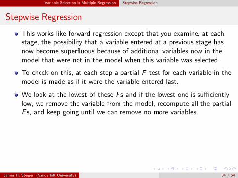
Variable Selection in Multiple Regression Stepwise Regression
Stepwise Regression
This works like forward regression except that you examine, at eachstage, the possibility that a variable entered at a previous stage hasnow become superfluous because of additional variables now in themodel that were not in the model when this variable was selected.
To check on this, at each step a partial F test for each variable in themodel is made as if it were the variable entered last.
We look at the lowest of these F s and if the lowest one is sufficientlylow, we remove the variable from the model, recompute all the partialF s, and keep going until we can remove no more variables.
James H. Steiger (Vanderbilt University) 34 / 54

Variable Selection in Multiple Regression Automatic Single-Term Sequential Testing in R
Automatic Sequential Testing of Single Terms
R will automatically perform a sequence of term-by-term tests on theterms in your model, in the order they are listed in the modelspecification.
Just use the anova command on the single full model.
You can prove for yourself that the order of testing matters, andsignificance level for a term’s model comparison test depends on theterms entered before it.
James H. Steiger (Vanderbilt University) 35 / 54

Variable Selection in Multiple Regression Automatic Single-Term Sequential Testing in R
Automatic Sequential Testing of Single Terms
For example, for the kids.data, we entered HGT first, then AGE ,and so our model was
> model.2 <- lm(WGT ~ HGT + AGE)
Here is the report on the sequential tests.
> anova(model.2)
Analysis of Variance Table
Response: WGT
Df Sum Sq Mean Sq F value Pr(>F)
HGT 1 589 589 27.12 0.00056 ***
AGE 1 104 104 4.78 0.05649 .
Residuals 9 195 22
---
Signif. codes:
0 '***' 0.001 '**' 0.01 '*' 0.05 '.' 0.1 ' ' 1
Notice that HGT , when entered first, has a p-value of .0005582.
James H. Steiger (Vanderbilt University) 36 / 54
Variable Selection in Multiple Regression Automatic Single-Term Sequential Testing in R
Automatic Sequential Testing of Single Terms
Next, try a model with the same two variables listed in reverse order.
R will test the terms with sequential difference tests, and now thep-value for HGT will be higher.
In colloquial terms, HGT is “less significant” when entered after AGE ,because AGE can predict much of the variance predicted by HGT andso HGT has much less to add after AGE is already in the equation.
> model.2b <- lm(WGT ~ AGE + HGT)
> anova(model.2b)
Analysis of Variance Table
Response: WGT
Df Sum Sq Mean Sq F value Pr(>F)
AGE 1 526 526 24.24 0.00082 ***
HGT 1 166 166 7.66 0.02181 *
Residuals 9 195 22
---
Signif. codes:
0 '***' 0.001 '**' 0.01 '*' 0.05 '.' 0.1 ' ' 1
James H. Steiger (Vanderbilt University) 37 / 54

Variable Selection in Multiple Regression Automatic Single-Term Sequential Testing in R
Automatic Sequential Testing of Single Terms> summary(model.2b)
Call:
lm(formula = WGT ~ AGE + HGT)
Residuals:
Min 1Q Median 3Q Max
-6.871 -1.700 0.345 1.464 10.234
Coefficients:
Estimate Std. Error t value Pr(>|t|)
(Intercept) 6.553 10.945 0.60 0.564
AGE 2.050 0.937 2.19 0.056 .
HGT 0.722 0.261 2.77 0.022 *
---
Signif. codes:
0 '***' 0.001 '**' 0.01 '*' 0.05 '.' 0.1 ' ' 1
Residual standard error: 4.66 on 9 degrees of freedom
Multiple R-squared: 0.78,Adjusted R-squared: 0.731
F-statistic: 16 on 2 and 9 DF, p-value: 0.0011
James H. Steiger (Vanderbilt University) 38 / 54

Variable Selection in Multiple Regression Automatic Single-Term Sequential Testing in R
Automatic Sequential Testing of Single TermsNotice also that the difference test p-value for the last variableentered is the same as the p-values reported in the overall output forthe full model, but, in general, the other p-values will not be thesame.
> anova(model.2b)
Analysis of Variance Table
Response: WGT
Df Sum Sq Mean Sq F value Pr(>F)
AGE 1 526 526 24.24 0.00082 ***
HGT 1 166 166 7.66 0.02181 *
Residuals 9 195 22
---
Signif. codes:
0 '***' 0.001 '**' 0.01 '*' 0.05 '.' 0.1 ' ' 1
> summary(model.2b)
Call:
lm(formula = WGT ~ AGE + HGT)
Residuals:
Min 1Q Median 3Q Max
-6.871 -1.700 0.345 1.464 10.234
Coefficients:
Estimate Std. Error t value Pr(>|t|)
(Intercept) 6.553 10.945 0.60 0.564
AGE 2.050 0.937 2.19 0.056 .
HGT 0.722 0.261 2.77 0.022 *
---
Signif. codes:
0 '***' 0.001 '**' 0.01 '*' 0.05 '.' 0.1 ' ' 1
Residual standard error: 4.66 on 9 degrees of freedom
Multiple R-squared: 0.78,Adjusted R-squared: 0.731
F-statistic: 16 on 2 and 9 DF, p-value: 0.0011
James H. Steiger (Vanderbilt University) 39 / 54

Variable Selection in R Problems with Statistical Testing in the Variable Selection Context
Problems with Statistical Testing
Frequently multiple regressions are at least partially exploratory innature.
You gather data on a large number of predictors, and try to build amodel for explaining (or predicting) y from a number of x ’s.
A key aspect of this is choosing which x ’s to retain.
A key problem is that, especially when n is small and the number ofx ’s is large, there will be a number of spuriously large correlationsbetween the criterion and the x ’s.
You can capitalize on chance, as it were, and build a regressionequation using variables that have high correlations with the criterion,but this equation will not generalize to any new situation.
James H. Steiger (Vanderbilt University) 40 / 54

Variable Selection in R Problems with Statistical Testing in the Variable Selection Context
Problems with Statistical Testing
There are a number of statistical tests available in multiple regression,and they are printed routinely by statistical software such as SPSS,SAS, Statistica, SPLUS, and R.
It is important to realize that these test do not in general correct forpost hoc selection.
So, for example, if you have 90 potential predictors that all actuallycorrelate zero with the criterion, you can choose the predictor withthe highest absolute correlation with the criterion in your currentsample, and invariably obtain a “significant” result.
Strangely, this fact is seldom brought to the forefront in textbookchapters on multiple regression.
Consequently, people actually believe that the F statistics andassociated probability values somehow determine whether theregression equation is significant in the sense most relatively naiveusers would expect.
James H. Steiger (Vanderbilt University) 41 / 54

Variable Selection in R Problems with Statistical Testing in the Variable Selection Context
Demonstration: Forward Regression with RandomUncorrelatedPredictors
We can demonstrate how Forward Regression or Stepwise Regressioncan produce wrong results.
We begin by creating a list of names for our variables.
> names <- c("Y", paste("X", 1:90, sep = ""))
Then we create a data matrix of order 50× 91 containing totallyindependent normal random numbers.
> set.seed(12345) #so we get the same data
> data <- matrix(rnorm(50 * 91), 50, 91)
Then I add the column names to the data and turn the data matrixinto a dataframe.
> colnames(data) <- names
> test.data <- data.frame(data)
> attach(test.data)
Note that these data simulate samples from a population whereR2 = 0, as all the variables are uncorrelated.
James H. Steiger (Vanderbilt University) 42 / 54
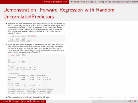
Variable Selection in R Problems with Statistical Testing in the Variable Selection Context
Demonstration: Forward Regression with RandomUncorrelatedPredictors
We start the forward selection procedure (which is fully automated bySPSS) by looking for the X predictor that correlates most highly withthe criterion variable Y . We can examine all the predictor-criterioncorrelations, sorted, using the following command, which grabs thefirst column and sorts its entries, then restrict the output to thelargest 3 values:
> sort(cor(test.data)[, 1])[88:91]
X48 X77 X53 Y
0.2568 0.3085 0.3876 1.0000
Since we have been privileged to examine all the data and select thebest predictor, the probability model on which the F -test for overallregression is based is no longer valid. We can see that X 53 has acorrelation of .388, despite the fact that the population correlation iszero. Here is the evaluation of model fit:
> summary(lm(Y ~ X53))
Call:
lm(formula = Y ~ X53)
Residuals:
Min 1Q Median 3Q Max
-2.171 -0.598 0.106 0.601 1.998
Coefficients:
Estimate Std. Error t value Pr(>|t|)
(Intercept) 0.189 0.144 1.31 0.1979
X53 0.448 0.154 2.91 0.0054 **
---
Signif. codes:
0 '***' 0.001 '**' 0.01 '*' 0.05 '.' 0.1 ' ' 1
Residual standard error: 1.02 on 48 degrees of freedom
Multiple R-squared: 0.15,Adjusted R-squared: 0.133
F-statistic: 8.49 on 1 and 48 DF, p-value: 0.00541
The regression is “significant” beyond the .01 level.
James H. Steiger (Vanderbilt University) 43 / 54

Variable Selection in R Problems with Statistical Testing in the Variable Selection Context
Demonstration: Forward Regression with RandomUncorrelatedPredictors
The next largest correlation is X77. Adding that to the equationproduces a “significant” improvement, and an R2 value of 0.26.
> summary(lm(Y ~ X53 + X77))
Call:
lm(formula = Y ~ X53 + X77)
Residuals:
Min 1Q Median 3Q Max
-2.314 -0.626 0.100 0.614 1.788
Coefficients:
Estimate Std. Error t value Pr(>|t|)
(Intercept) 0.211 0.136 1.55 0.1284
X53 0.471 0.145 3.24 0.0022 **
X77 0.363 0.137 2.65 0.0110 *
---
Signif. codes:
0 '***' 0.001 '**' 0.01 '*' 0.05 '.' 0.1 ' ' 1
Residual standard error: 0.963 on 47 degrees of freedom
Multiple R-squared: 0.261,Adjusted R-squared: 0.229
F-statistic: 8.28 on 2 and 47 DF, p-value: 0.00083
It is precisely because F tests perform so poorly under theseconditions that alternative methods have been sought. Although Rimplements stepwise procedures in its step library, it does not use theF -statistic, but rather employs information-based criteria such as theAIC.
In its leaps procedure, R implements an “all-possible-subsets” searchfor the best model.
We shall examine the performance of some of these selectionprocedures in Homework 5.
James H. Steiger (Vanderbilt University) 44 / 54

Information-Based Selection Criteria The Active Terms
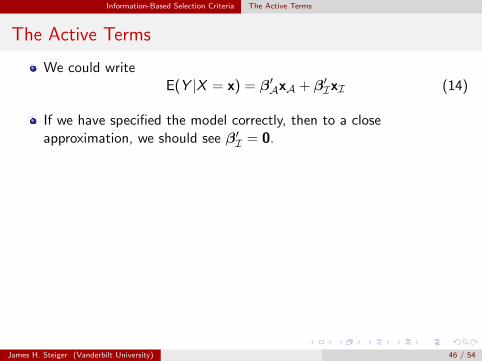
The Active Terms
One way of conceptualizing variable selection is to parse the availableterms in the analysis into active and inactive groups.
A simple notation for describing this is as follows:
Given a response Y and a set of terms X , the idealized goal ofvariable selection is to divide X into two pieces, i.e., X = (XA,XI),where XA is the set of active terms, and XI is the set of inactiveterms not needed to specify the mean function.
E(Y |XA,XI) and E(Y |XA) would give the same results.
James H. Steiger (Vanderbilt University) 45 / 54
Information-Based Selection Criteria The Active Terms
The Active Terms
We could writeE(Y |X = x) = β′AxA + β′IxI (14)
If we have specified the model correctly, then to a closeapproximation, we should see β′I = 0.
James H. Steiger (Vanderbilt University) 46 / 54
Information-Based Selection Criteria Information Criteria
Information Criteria
Suppose that we have a candidate subset XC , and that the selectedsubset is actually equal to the entire set of active terms XA.
Then, of course (depending on sample size) the fit of the meanfunction including only XC should be similar to the fit of the meanfunction including all the non-active terms.
If XC misses important terms, the residual sum of squares should beincreased.
James H. Steiger (Vanderbilt University) 47 / 54

Information-Based Selection Criteria Information Criteria
Information CriteriaThe Akaike Information Criterion (AIC)
Criteria for comparing various candidate subsets are based on the lackof fit of a model in this case, as assessed by the residual sum ofsquares (RSS), and its complexity, assessed by the number of terms inthe model.
Ignoring constants that are the same for every candidate subset, theAIC, or Akaike Information Criterion, is
AICC = n log(RSSC/n) + 2pC (15)
According to the Akaike criterion, the model with the smallest AIC isto be preferred.
James H. Steiger (Vanderbilt University) 48 / 54

Information-Based Selection Criteria Information Criteria
Information CriteriaThe Schwarz Bayesian Criterion
This criterion is
BICC = n log(RSSC/n) + pC log(n) (16)
James H. Steiger (Vanderbilt University) 49 / 54

Information-Based Selection Criteria Information Criteria
Information Criteria
Mallows Cp criterion is defined as
CpC =RSSCσ2
+ 2pC − n (17)
where σ2 is obtained from the fit of the model with all terms included.
Note that, for a fixed number of parameters, all three criteria aremonotonic in RSS .
James H. Steiger (Vanderbilt University) 50 / 54

(Estimated)Standard Errors
Estimated Standard Errors
Along with other statistical output, statistical software typically canprovide a number of “standard errors.”
Since the estimates associated with these standard errors areasymptotically normally distributed, the standard errors can be usedto construct Wald Tests and/or confidence intervals for thehypothesis that a parameter is zero in the population.
Typically, software does not provide a confidence interval for R2 itself,or even a standard error.
The calculation of an exact confidence interval for R2 is possible, andRachel Fouladi and I provided the first computer program to do that,in 1992.
James H. Steiger (Vanderbilt University) 51 / 54
Standard Errors for Predicted and Fitted Values
Standard Errors for Predicted and Fitted Values
Recall that there are two related but distinct goals in regressionanalysis. One goal is estimation: from the data at hand, we wish todetermine an optimal predictor set and accurately estimate β weightsand R2
pop.
Another goal is prediction, and one variant of that involves estimationof β followed by the use of that β with a new set of observations x∗.We would like to be able to gauge how accurate our estimate of the(not yet observed) y∗ will be. Following Weisberg, we will refer tothose predictions as y∗.
James H. Steiger (Vanderbilt University) 52 / 54

Standard Errors for Predicted and Fitted Values
Standard Errors for Predicted and Fitted Values
In keeping with the above considerations, there are two distinctlydifferent standard errors that we can compute in connection with theregression line.
One standard error, sefit, deals with the estimation situation wherewe would like to compute a set of standard errors for the (population)fitted values on the regression line. This estimation of the conditionalmeans does not require a new x∗.
Another standard error, sepred, deals with the prediction situationwhere we have a new set of predictor values x∗, and we wish tocompute the standard error for the predicted value of y, i.e., y∗,computed from these values.
James H. Steiger (Vanderbilt University) 53 / 54
Standard Errors for Predicted and Fitted Values
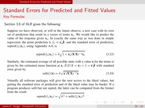
Standard Errors for Predicted and Fitted ValuesKey Formulas
Section 3.6 of ALR gives the following:
PROBLEMS 65
3.6 PREDICTIONS AND FITTED VALUES
Suppose we have observed, or will in the future observe, a new case with its ownset of predictors that result in a vector of terms x∗. We would like to predict thevalue of the response given x∗. In exactly the same way as was done in simpleregression, the point prediction is y∗ = x′∗β, and the standard error of prediction,sepred(y∗|x∗), using Appendix A.8, is
sepred(y∗|x∗) = σ
√1 + x′∗(X′X)−1x∗ (3.23)
Similarly, the estimated average of all possible units with a value x for the terms isgiven by the estimated mean function at x, E(Y |X = x) = y = x′β with standarderror given by
sefit(y|x) = σ√
x′(X′X)−1x (3.24)
Virtually all software packages will give the user access to the fitted values, butgetting the standard error of prediction and of the fitted value may be harder. If aprogram produces sefit but not sepred, the latter can be computed from the formerfrom the result
sepred(y∗|x∗) =√
σ 2 + sefit(y∗|x∗)2
PROBLEMS
3.1. Berkeley Guidance Study The Berkeley Guidance Study enrolled childrenborn in Berkeley, California, between January 1928 and June 1929, and thenmeasured them periodically until age eighteen (Tuddenham and Snyder, 1954).The data we use is described in Table 3.6, and the data is given in the datafiles BGSgirls.txt for girls only, BGSboys.txt for boys only, andBGSall.txt for boys and girls combined. For this example, use only thedata on the girls.
3.1.1. For the girls only, draw the scatterplot matrix of all the age two vari-ables, all the age nine variables and Soma. Write a summary of theinformation in this scatterplot matrix. Also obtain the matrix of samplecorrelations between the height variables.
3.1.2. Starting with the mean function E(Soma|WT9) = β0 + β1WT9, useadded-variable plots to explore adding LG9 to get the mean functionE(Soma|WT9, LG9) = β0 + β1WT9 + β2LG9. In particular, obtain thefour plots equivalent to Figure 3.1, and summarize the information inthe plots.
3.1.3. Fit the multiple linear regression model with mean function
E(Soma|X) = β0 + β1HT2 + β2WT2 + β3HT9 + β4WT9 + β5ST9(3.25)
James H. Steiger (Vanderbilt University) 54 / 54