Introduction to Inertial Navigation and Pointing Control

Zhang Liu

Guidance Navigation Control Engineer

Northrop Grumman, San Diego, CA

December 15, 2011

Outline

• Inertial Navigation System (INS)

• INS/GPS Integration

• Pointing Control System

2

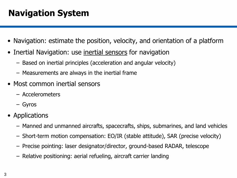
Navigation System

• Navigation: estimate the position, velocity, and orientation of a platform

• Inertial Navigation: use inertial sensors for navigation

– Based on inertial principles (acceleration and angular velocity)

– Measurements are always in the inertial frame

• Most common inertial sensors

– Accelerometers

– Gyros

• Applications

– Manned and unmanned aircrafts, spacecrafts, ships, submarines, and land vehicles

– Short-term motion compensation: EO/IR (stable attitude), SAR (precise velocity)

– Precise pointing: laser designator/director, ground-based RADAR, telescope

– Relative positioning: aerial refueling, aircraft carrier landing

3

Common Sensor Error Terms

• Use weight scale as an example to explain common sensor error terms

– Weight = Spring Constant * Distance Deflection

– Ex: 100 lb = 100 * 1 cm 200 lb = 100 * 2 cm

• Bias Error – An added constant, independent of input

– Weight = Spring Constant * Distance Deflection + Bias

– Ex: 102 lb = 100 * 1 cm + 2 202 lb = 100 * 2 cm + 2

• Scale Factor Error – proportional to input

– Sprint constant is the scale factor in our example

– Ex: 103 lb = 101 * 1 cm + 2 204 lb = 101 * 2 cm + 2

• Noise – fast changing random effect

– Zero-mean random variable, certain probability distribution

– Random Walk: phenomena when integrating noise over time

• Linearity Error – input-output nonlinearity

– Ideally, input-output plot is a straight line

• Misalignment – Difference between actual sensing axis and perceived sensing axis 4

0 100 200 300-15

-10

-5

0

5

10

15

Noise

Random Walk

0 20 40 60 80 1000

20

40

60

80

100

Accelerometers

• Measure specific force

– Specific force = acceleration - gravity

• Error sources: bias, scale factor, misalignment, linearity, random walk

• Bias is typically the dominant error source

– Navigation grade accelerometers have accuracy of 50 micro-g

– Simple 1-D model with a constant unknown bias term (No other aiding)

• Velocity can be obtained by integrating the acceleration

• Position can be obtain by integrating the velocity

5

atruemeas baa

tbvvavv atrue

t

measest 00

0

2

000

02

1tbtvppvpp atrue

t

estest

Unbounded Drift Error

Accelerometer Technology Application

6

Figure: Schmidt (2011)

• Measure angular velocity

• Error sources: bias, scale factor, misalignment, linearity, random walk

• Bias is typically the dominant error source

– Navigation grade gyros have accuracy of 0.01 °/hr

– Simple 1-D model with a constant unknown bias term (No other aiding)

• Attitude (Orientation) can be obtained by integrating the angular velocity

Gryos

7

gtruemeas b

tbgtrue

t

measest 00

0

Mechanical Gyros Maintain angular momentum

Ring Laser or Fiber Optic Gyros Sagnac Effect: Light Interference Pattern

MEMS Gyros Coriolis Effect

Unbounded Drift Error

Gyro Technology Application

8

Earth Rate 1 nmi/hr Free Inertial Drift

Figure: Schmidt (2011)

Inertial Measurement Unit (IMU)

• Typically an IMU has 3 accelerometers and 3 gyros (x, y, z)

• Strapdown IMU – All inertial sensors are rigidly attached to the platform (no mechanical movement)

– Almost all IMUs on the market today are strapdown systems

– Example:

Honeywell HG1700 AG58 (Tactical Grade)

• Gyros accuracy: 1 deg/hr

• Accelerometers accuracy: 1 mg

• Gimballed IMU – Gyros and accelerometers are isolated from movement by means of gimbals

– Big, heavy, and very expensive to make and maintain

– Only used when the highest possible accuracy is required

– Example:

SPIRE System

9

IMU Performance and Application

10

Strategic Grade/High

Performance

Navigation

Grade/Medium

Performance Inertial AHRS Grade Tactical Grade Flight Control

Performance < 1.0 nmph CEP

< 1.0 mil pointing 2 - 5 mil heading

Bias deg/hr 0.001 - 0.005 0.003 - 0.01 0.05 - 3.0 5 - 50 100

Scale Factor ppm 1 - 10 10 - 30 100 - 500 500 - 1500 2000

Angle Random

Walk deg/√Hz 0.00001 - 0.0005 0.001 - 0.002 0.005 - 0.05 0.1 - 0.5 1.0

Bias μg 0.1 - 10 20 - 50 100 - 500 500 - 1,000 1,500

Scale Factor ppm 0.1 - 10 40 - 150 300 - 900 1,000 - 3,000 5000

Angle Random

Walk μg/√Hz 2 - 5 5 - 20 25 - 40 50 - 75 100

Stabilization Inertial Navigation

Attitude & Heading

Reference

Missile Midcourse

guidance Rate monitoring

Pointing & Slewing Air Gimbal Stabilization Munitions guidance

Orbit Correction Land Sensor Pointing

Marine SAR Velocity Ref

Strategic Plaform

Navigation Pointing

GY

RO

Acc

el

Inertial Sensor Performance Across Applications

Ap

pli

cati

on

s

Inertial Navigation System (INS)

• An INS consists of a IMU and a system processor

• The system processor computes the solution (position, velocity, attitude)

– Due to errors in gyros and accelerometers, the solution has unbounded drift error

• Strap-down INS integration equations

11

e

nn

Ce

nn

Up

n

C

n

e

n vMvuFZn

)(

3-axis Gyros

n

b

e

i

nn

e

nb

i

bn

b

n

b CCCdt

d )(

e

nC

l

nn

e

nn

e

ne

i

nb

i

bn

b

n

e

n gvfCvdt

d

)2( 3-axis

Accelerometers

b

i

b f

n

bC

dt )(

n

e

nv

dt )(

n

bC

n

e

nv

dt )(

e

n

n

e

ne

n CCdt

d][

e

i

eTe

n

e

i

n C

)(

n

e

n

e

i

n

b

i

b

dt )(n

e

nr

INS Aidings

• Inertial sensors can accurately capture high-frequency dynamics

• To limit drift error in the integrated solution, an INS requires aiding

12

Aiding System Measurement

GPS Pseudo range, delta pseudo range

Star tracker Attitude orientation

Receive signal strength Attitude orientation

Image Correlation (EO/IR) Attitude orientation

Multi-antenna GPS Attitude orientation

Barometer Altitude

Magnetometer / Compass Heading

Doppler radar velocity

Underwater pressure sensor Depth

Underwater transponder Range from known position

Outline

• Inertial Navigation System (INS)

• INS/GPS Integration

• Pointing Control System

13

One Dimensional Example (Part 1) -- A car with one accelerometer driving on a perfectly straight road

-- GPS aiding, naïve open loop design

14

True

Acceleration

+

+

Noise

σ = 0.001 m/s^2

Bias

0.01 m/s^2

100 Hz

Integrate

11 z

Ts

Accel-only

Velocity

Integrate

11 z

Ts

Accel-only

Position

True

Velocity

Bias

3 m

Noise

σ = 0.1 m/s

1 Hz

+

+

Linear Extrapolation 100 Hz

True

Position

+

+ 1 Hz

Integrate

11 z

Ts

Hybrid

Velocity Integrate

11 z

Ts

Hybrid

Position

GPS-only

Position

Reset Initial

Condition Reset Initial

Condition

100

1i

sT Sum

Over 1s

11 zDiff

Over 1s

−

+ Accel Bias

Estimate Moving Average

One Dimensional Example (Part 2) -- A car with one accelerometer driving on a perfectly straight road

-- GPS aiding, naïve open loop design using two 1st order filters

15

0 20 40 60-10

-5

0

5

10

Time (s)

True Acceleration (m/s 2)

0 20 40 600

20

40

60

80

100

120

Time (s)

True Velocity (m/s)

0 20 40 600

500

1000

1500

2000

2500

3000

Time (s)

True Position (m)

0 20 40 60-5

0

5

10

15

20

Time (s)

Standalone Position Error (m)

0 20 40 602.7

2.8

2.9

3

3.1

3.2

Time (s)

Hybrid Position Error (m)

0 20 40 60-0.4

-0.2

0

0.2

0.4

0.6

Time (s)

Accel Bias Estimate (m/s 2)

Accel only

GPS only

Before Moving Average

After Moving Average

True Value

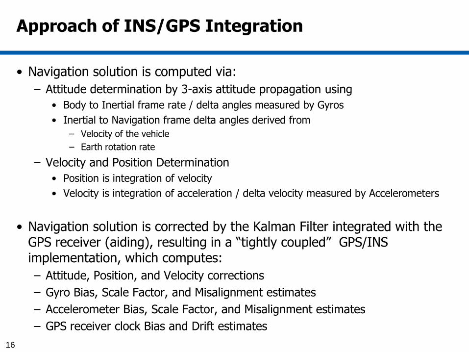
Approach of INS/GPS Integration

• Navigation solution is computed via:

– Attitude determination by 3-axis attitude propagation using

• Body to Inertial frame rate / delta angles measured by Gyros

• Inertial to Navigation frame delta angles derived from

– Velocity of the vehicle

– Earth rotation rate

– Velocity and Position Determination

• Position is integration of velocity

• Velocity is integration of acceleration / delta velocity measured by Accelerometers

• Navigation solution is corrected by the Kalman Filter integrated with the GPS receiver (aiding), resulting in a “tightly coupled” GPS/INS implementation, which computes:

– Attitude, Position, and Velocity corrections

– Gyro Bias, Scale Factor, and Misalignment estimates

– Accelerometer Bias, Scale Factor, and Misalignment estimates

– GPS receiver clock Bias and Drift estimates

16

Tightly-Coupled INS/GPS Architecture

17

IMU (Gyro & Accels)

Delta Angle (rate) & Delta Velocity

(accel) Correction by estimated bias,

Scale factor & misalignments

Attitude Velocity & Position

Correction

Predicted Pseudo Range Computation

Position

Predicted Delta Range

Computation

Velocity

-

-

Multiply By

Kalman Filter Gains

Kalman Filter Covariance

Propagation Gain Computation

& Covariance Update

Non-Linear Navigation Integration

Pseudo Range Residual

Delta Range Residual

Estimated Gyro & Accelerometer Bias, Scale factor & Misalignment

Position Velocity & Attitude Corrections

Clock Rate correction

Clock bias correction

Compute A-matrix

GPS Receiver

Pseudo Range

Compute H-matrix

Delta Range

Delta Velocity Delta Angle

Position Velocity & Attitude

Angular Rate Linear Acceleration

INS/GPS Kalman Filter: States

18

gpsr

acc

gyro

n

e

n

n

n

x

x

x

r

v

X

ˆ

32 states # Total

(1x1) drift,clock receiver GPS :

(1x1) ,clock bias receiver GPS : ] ,[

)1(3 ignment,ity misalorthogonal- nonaccel. :

(3x1) , factorsscaled accel. :

(3x1) frame, body , ter biasaccelerome : ],,[

1)(3 gnment,ity misaliorthogonal- nongyro :

1)(3 ent, misalignml rotationagyro :

1),(3 factors,scaled gyro :

(3x1), frame body bias,gyro : ],,,[

1)(3 frm.on navigati:error position

1)(3 frm.n navigatio,],,[ :error velocity

1)(3 framen navigatioerror, attitude

b

m

m

ˆ

r

rrr

T

gpsr

a

a

aaaa

bT

acc

g

g

g

b

ggg

bT

gyro

n

T

DEN

n

n

n

t

tttx

S

bSbx

S

bSbx

r

vvvv

g

g

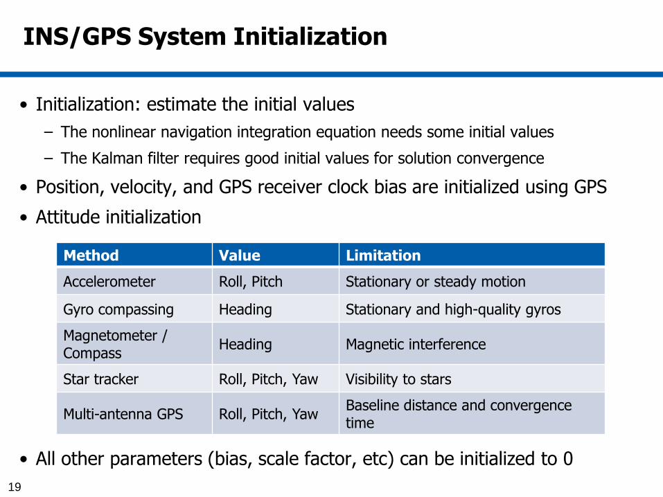
INS/GPS System Initialization

19

• Initialization: estimate the initial values

– The nonlinear navigation integration equation needs some initial values

– The Kalman filter requires good initial values for solution convergence

• Position, velocity, and GPS receiver clock bias are initialized using GPS

• Attitude initialization

• All other parameters (bias, scale factor, etc) can be initialized to 0

Method Value Limitation

Accelerometer Roll, Pitch Stationary or steady motion

Gyro compassing Heading Stationary and high-quality gyros

Magnetometer / Compass

Heading Magnetic interference

Star tracker Roll, Pitch, Yaw Visibility to stars

Multi-antenna GPS Roll, Pitch, Yaw Baseline distance and convergence time

Outline

• Inertial Navigation System (INS)

• INS/GPS Integration

• Pointing Control System

20

Feedback Control

• Example

– Consumer: temperature control (oven, A/C), cruise control, hard disk arm control

– Defense: missile guidance, flight control, attitude control, pointing control

• Why do we need feedback?

– To deal with Uncertainty

• Approximate model of the system dynamics

• Unknown disturbance and noise

21

Desired Output

Controller System

Actual Output

+ −

Feedback loop

Disturbance

Noise

Measured Output

Sensor

Control Methods

• Classic Control

– Deal with single-input single-output (SISO) system

– Based on transfer function (zeros/poles) or impulse response model

– PID control, Lead-Lag compensator

• PID is by far the most widely known and used control technique in practice

– For many multi-input multi-output (MIMO) systems in practice, can decouple to multiple SISO systems

• Moderm Control

– Based on state-space model that naturally includes MIMO case

– Linear Quadratic Regulator (LQR)

– LQG, H∞ and robust control

• Nonlinear Control

– Bang-Bang Control (on/off)

– Lyapunov function, Pontryagin's minimum principle

• Others

– Adaptive Control, Model Predictive Control

– Distributed Control, Cooperative Control, Hybrid Control

– …

22

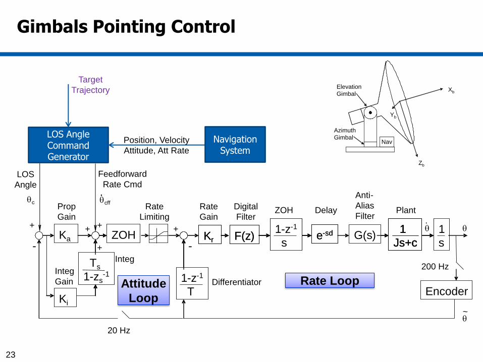
Gimbals Pointing Control

23

Rate Loop

K r F(z ) e - sd 1 - z - 1

s

1

Js+c

1

s

Encoder 1 - z - 1

T

G(s )

Differentiator

Digital

Filter ZOH Delay

Anti -

Alias

Filter Rate

Gain Plant

.

200 Hz

~

K a

Prop

Gain

K i

ZOH

T s

1 - z s - 1

c

20 Hz

cff .

- -

+ + + +

+

Integ

Integ

Gain

Rate

Limiting

K r F(z ) e - sd 1 - z - 1

s

1 - z - 1

s

1

Js+c

1

Js+c

Attitude

Loop

LOS Angle Command Generator

LOS

Angle

Feedforward

Rate Cmd

Target

Trajectory

Position, Velocity

Attitude, Att Rate

Navigation System

X b

Y b

Z b

Elevation Gimbal

Azimuth

Gimbal Nav

Laser Pointing

• Laser pointing requires very accurate pointing (< 0.005°)

– Laser has a much narrower beam width than RF

– Ex: Inter-satellite communication, directed energy weapon

• Coarse Pointing - Gimbals

– Use conventional electrical motors

– Sufficient for acquisition and tracking

– Control bandwidth: 5 – 50 Hz

• Fine Pointing - Mirrors

– Use piezoelectric or ultrasonic motor

– Use 4-quadrants detector to provide feedback

– Very high resolution (arc-sec)

– Can achieve control bandwidth > 1000 Hz

24

Guelman 2004

• Mechanical misalignment

– Design online / offline calibration methods to estimate the misalignment and lever arm between the navigation system and payload pointing system

– Ex 1: Use received signal strength in communication pointing

– Ex 2: Use image correlation in camera (EO/IR) pointing

– Ex 3: Install low quality IMU on the payload pointing system (Transfer Align, Velocity Matching)

• Better model of unknown disturbance

– Ex 1: Periodic vibration

– Ex 2: Reaction wheel in spacecraft

– Ex 2: Time-correlated (Non-white)

• Compensate delay by extrapolation

– Accurate data time tag

– Linear or quadratic extrapolation

25

Time

Att

itude

extrapolation

hold

n+1(actual)

n

n-1

Extrapolation error

Hold error

0 100 200 300 400 500 600-0.6

-0.4

-0.2

0

0.2

0.4

Yaw

(deg)

Time (sec)

0 100 200 300 400 500 600-0.4

-0.2

0

0.2

0.4

Pitch (

deg)

without extrapolation

with extrapolation

0 100 200 300 400 500 600-0.2

-0.1

0

0.1

0.2

Roll

(deg)

Errors due to a 1 Sample Delay w/ & w/o Extrapolation, File:car test 1 20041128 5

Example

Example

Model Fidelity

Encoder outputs on the Gimbals match IMU outputs after misalignment calibration

Conclusion

26

Thank you for your interest

• This brief presentation covers some basic principles in the inertial navigation system and the pointing control system.

• Further references – Inertial Navigation

• D. Titterton and J. Weston, Strapdown Inertial Navigation Technology

• J. Farrell, Aided Navigation

– Automatic Control

• D.G. Luenberger, Introduction to Dynamic Systems

• Anderson and Moore, Linear Optimal Control

• S. Sastry, Nonlinear systems: Analysis, Stability, and Control