free-inertial and damped-inertial navigation mechanization and

AD-A014 356

FREE-INERTIAL AND DAMPED-INERTIALNAVIGATION MECHANIZATION AND ERROREQUATIONS

Warren G. Heller

Analytic Sciences Corporation

Prepared for:

Defense Mapping Agency Aerospace Center

18 April 1975

DISTRIBUTED BY:

National Technical Information ServiceU. S. DEPARTMENT OF COMMERCE

Si

swof

IHI

IL JI

-J THE ANALYTIC SCIENCES CORPORATION

TR-312-1-1

FREE-INERTIAL AND DAMPED-INERTIALNAViGATION MECHANIZATION AND

ERROR EQUATIONS

Ap~ril 18, 19715

Prepared under.Contract No. DMA700-74-C-0075

for

Defense Mapping Agency Aerospace CenterSt. Louis Air Force Station

Missouri 63118

Prepared by:

D D Warren G. Heller

Approved by:

Stanley K. Jordan

U L36.Raymnond A. Nash, Jr.

THE ANALYTIC SCIENCES CO1PQORATION6 Jacob Wtv

Reading, Massachiusetts 01867

UNCLASSIFIE -.4SECURITY CLASSIFICATION OF TMIS PAGE fftli Datais gtere.

READ TNSTRUC-ONREPORT DOCUMENTATION PAGE BEFORE COMPLETING FORM -AV. FVP011 NOW'111'E1 '1. GOVT ACCESSION NO RE. MICIPIENT'S CATALOG NUMdgER -

TASC Number TR-312-1-1 Inone assigned __ _

S. TITL l Stle) 5 TYPE OFRK"P R TA PERIOO COVC/REO

Fr-,- 1wer l and Dmped-Inertial Navigation TechnicalMechanization and Error Equations 8/20-73 - 8/20/74

S. PjLtFORJ4djNjOjO, REPORT NUMSERATR-31_. -l

7. AUTHOR(a) I. CONTRACT OR GRANT NUMBER(sj

Warren G. Holler OKA 700-74-C-0075., PERPORIING ORGANIZATION NAME AND ADDRESS 16. PROGRAM ELEMENT, PROJECT, TASK

The Analytlc Sciences Corporation AREA & WORK UNIT NUMBERS

6 Jacob WayRedi ng, MA 01867 Does not apply

1i. CONTROL.ING OFFICE NAME AND ADDRESS 12. REPORT DATE

Defense Mapping Agency Aerospace Center 18 Apr 75ATTN: PRA 13.NUMBR OF PAGESSt Louis AFS, MO 63118 5.7

14. MONITORING AGENCY NAME I ADDRESS(II different from Conttrolling Office) 15. SECURITY CLASS. (of this report)

tiUNCLASSIFIEDSame as item Ill

15.. OECLASSI FICATION 'DOWN GRADINGSCHEDULE

1I. OISTRi•5UTION STATEMENT (of thia Report)

Approved for public release; distribution unlimited.

17ý DISTRIBUTION STATEMENT (of the abslract enttered In Block 20, If different from Report)

Sam IIIS, SUPPLEMENTARY NOTES

None

It KEY WORDS (Continue on forerie aid@ if neceaesry and Identify by, block number)

Inertial Navigation, Aided Inertial, Error Equations

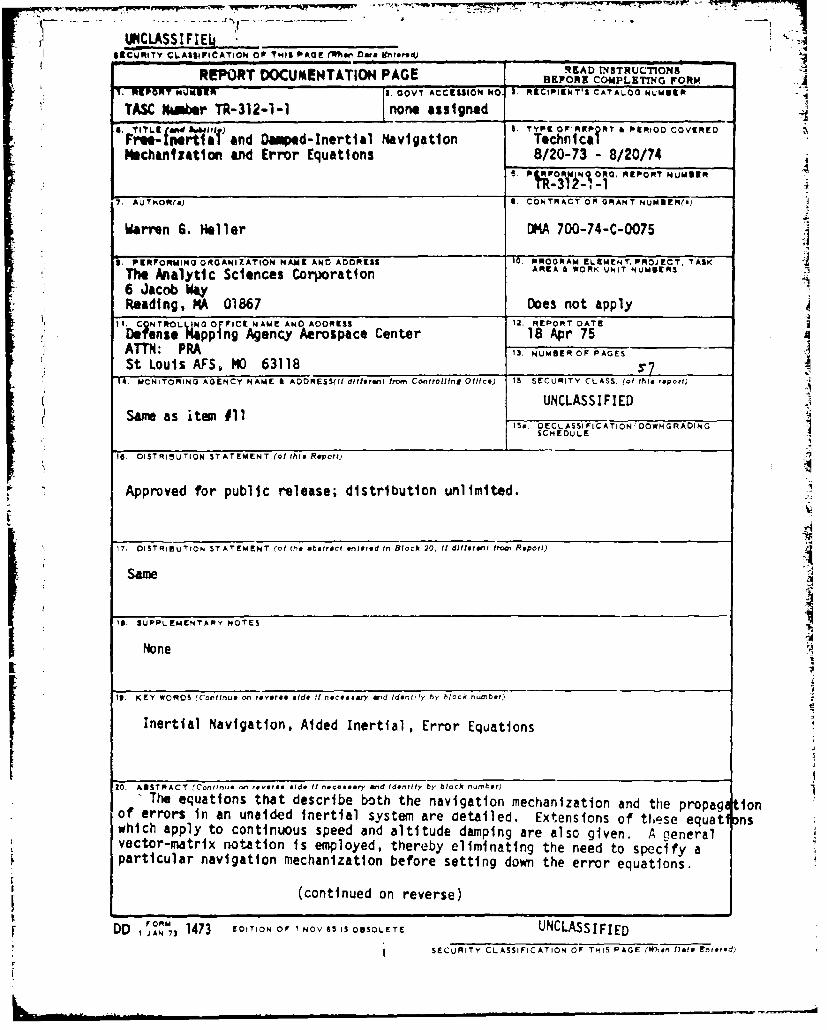
20. ABSTRACT rContinu0 on #eeores Sd* If nececeery and Identify by block nr nber)

The equations that describe both the navigation mechanization and the propaga ionof errors in an unaided inertial system are detailed. Extensions of these equationswhich apply to continuous speed and altitude damping are also given. A generalvector-matrix notation is employed, thereby eliminating the need to specify aparticular navigation mechanization before setting down the error equations.

(continued on reverse)

DD 04m 1473 EDITION O1 I'NOV 6 IS OBSOLETE UNCLASSIFIEDSECURITY CLASSIFICATION OF THIS PAGE (*10,n Date Ent.,ed)

- ---- ---

84COY,"AWPLATIOW OF 1.Nil PAOU 004 bie0e1dj

'#20 (cont'd)I--Sp~acific application of t~he 9 teral equations to the local-level, wanger-A

azimuth mechanization is outlined Tim detailed form of the errei' equationsAis given for both the free-inerti case and various cholc*n of continuous

do~ing.

SECRIY CASIFIATON F WSP.G~rhenDaa E~ovd

kL_

THE ANALYTIC SCIENCES CORPORATION

FOREWORD

i This document contains the first subset of equationsto be furnished to the Defense Mapping Agency AerospaceCenter (DMAAC) as a part of Task II of contract iZMA700-74-C-0075, "Aided Inertial Navigation System Error Analysis."A total of three such equation subsets will be issued:

1. Free-Inertial and DaEnped-Inertial NavigationMechanization and Error Equations (the presentreport)

2. Covariance Propagation Equations for Optimaland Suboptimal Kalman-Filter-Integrated Multi-Sensor Inertial Systems

3. Models for Aided Inertial Navigation InstrumentErrors

The intent of these equation subsets is to provideDMAAC with complete, self-contained mathematical "modules"suitable for studying modern multi-sensor inertial navigationsystems such as those of the B-i and F-15 aircraft. Thesesubsets of equations are rendered in a form sufficiently generalas to be applicable to the inertial systems in all terrestrial

vehicles. Included in this category are missile, aircraft and,• marine naviqation. Also detailed is the particular form of theequations most suited to performance studies of these two

aircraft.

I

ii

i _ n nn -

.I THE ANALYTIC SCIENCES CORPORATION

.1

i ABSTRACTr

J

] The equations that describe both the navigationmechanization and the propagation of errors in an unaidedinertial system are detailed. Extensions of these equations

1 which apply to continuous speed and altitude damping arealso given. A general vector-matrix notation is employed,thereby eliminating the need to specify a particular naviga-tor mechanization before setting dovm the error equations.

-j

Specific application of the general equations to thelocal-level, wander-azimuth mechanization is outlined. Thedetailed form of the error equations is given for both thefree-inertial case and various choices of continuous damping.

I

iii


A

TABLE OF CONTENTS

PageNo.

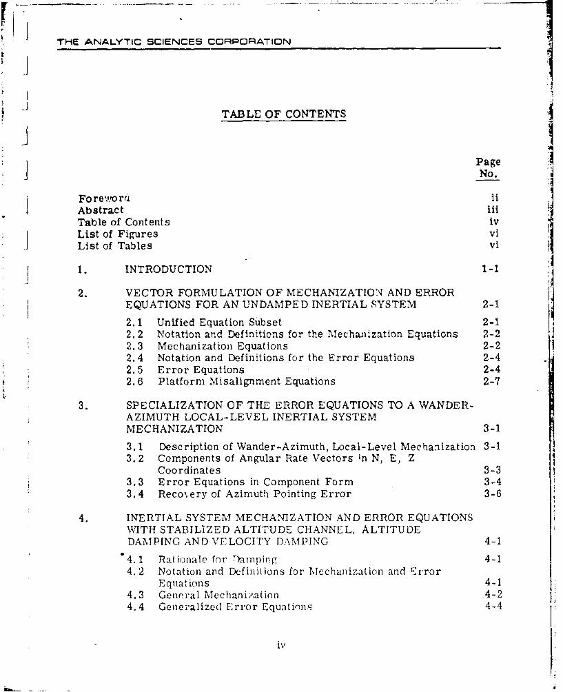
Fo reworr~i tAbstract iiiTable of Contents ivList of Figures viList of Tables vi

1. INTRODUCTION 1 -1

2. VECTOR FORMULATION OF MECHANIZATION AND ERROR- EQUATIONS FOR AN UNDAMPED INERTIAL SYSTEM 2-1

2.1 Unified Equation Subset 2-12.2 Notation and Definitions for the Mechanization Equations 2-22.3 Mechanization Equations 2-22.4 Notation and Definitions for the Error Equations 2-42.5 Error Equations 2-42.6 Platform Misalignment Equations 2-7

3. SPECIALIZATION OF THE ERROR EQUATIONS TO A WANDER-AZIMUTH LOCAL-LEVEL INERTIAL SYSTEMMECHANIZATION 3-1

3.1 Description of Wander-Azimuth, Local-Level Mechanization 3-13.2 Components of Angular Rate Vectors in N, E, Z

Coordinates 3-33.3 Error Equations in Component Form 3-43.4 Recoxery of Azimuth Pointing Error 3-6

4. INERTIAL SYSTEM MECHANIZATION AND ERROR EQUATIONSWITH STABILIZED ALTITUDE CHANNEL, ALTITUDEDAMPING AND VELOCITY DA\MPING 4-1

4.1 Rationale for Damping 4-14.2 Notation and Definitions fori Mechanization and Error

Equations 4-14.3 General Mechanization 4-24.4 Generalizect Error Equations 4-4

iv


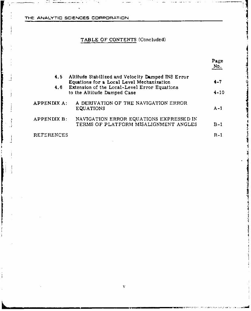
TABLE OF CONTENTS (Concluded)

IPageJNo.

4.5 Altitude Stabilized and Velocity Damped INS Error ]Equations for a Local Level Mechanization 4-7

4.6 Extension of the Local-Level Error Equationsto the Altitude Damped Case 4-10

APPENDIX A: A DERIVATION OF THE NAVIGATION ERROR IEQUATIONS A-i

APPENDIX B: NAVIGATION ERROR EQUATIONS EXPRESSED INj TERMS OF PLATFORM MISALIGNMENT ANGLES B-1

REFERENCES R-1

V


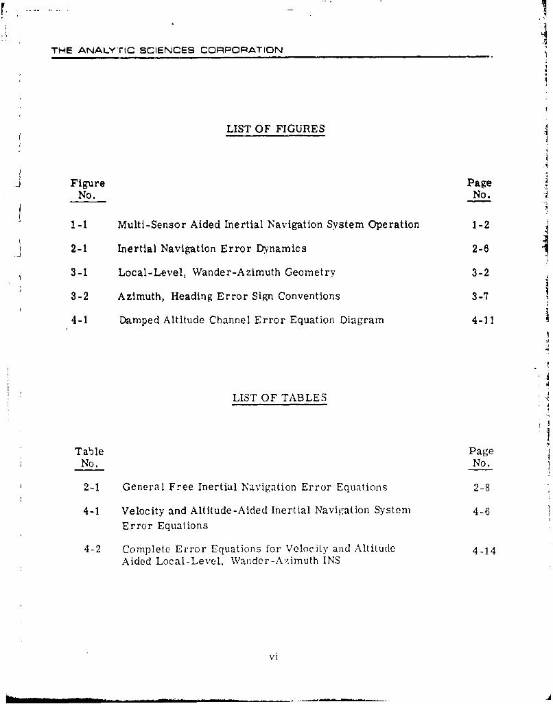
LIST OF FIGURES

Figure PageNo. No.

1-1 Multi-Sensor Aided Inertial Navigation System Operation 1-2

2-1 Inertial Navigation Error Dynamics 2-6

3-1 Local-Level, Wander-Azimuth Geometry 3-2

3-2 Azimuth, Heading Error Sign Conventions 3-7

4-1 Damped Altitude Channel Error Equation Diagram 4-11

LIST OF TABLES

Table PageNo. No.

2-I General Free Inertial Navigation Error Equations 2-8

4-1 Velocity and Altitude-Aided Inertial Navigation System 4-6

Error Equations

4-2 Complete Error Equations for Velocity and Altitude 4-14Aided Local-Level, Wander-A6,imuth INS

vi


1. INTRODUCTION

} The errors of an unaided inertial navigation system (INS) typically

grow with time in an unboundetý manner. As a consequence, the cruise inertial

navigation systems used in mcdern aircraft and submarines are normally aided

or "damped" with data from external aids, such as:

Saltim eter or depth gauge

* speed reference (doppler radar or EM-log)

* position reference (LORAN, NAVSAT, ... )

The errors of an aided INS are typically bounded, although the errors grow in-

between position fixes.

The techniques that are used to combbie external reference data with

INS outputs fall into two categories: "conventional continuous-feedback damp-

ing" and "Kalman-filter damping". Conventional continuous -feedback techniques

are usually used with altitude and speed reference devices, whereas Kalman-

filter techniques are frequently used with position reference devices. However,

the trend in recent years has been toward more extensive use of Kalman-

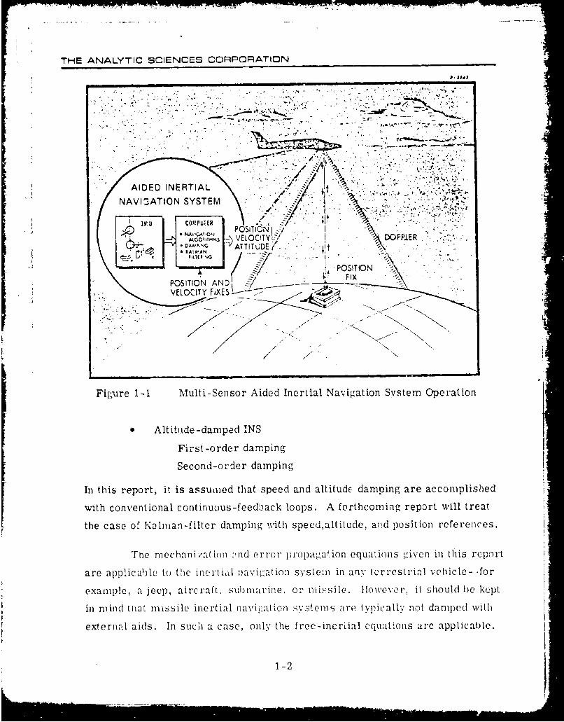
filter techniques. An overall conceptual diagram of a multi-sensor aided INS

is shown in Fig. 1-1.

The purpose of this report is to present the mechanization and linear-

ized error propagation equations for the following cases:

"* Unaided INS

"* Speed-damped INS

First-order damping..

Second-order damrping

1-1


v; e,6

All~tSV*

AW.OITM VEOCT DOPLE

NAPOSITION SYSTE FIX

VELOCITY FiXES<

I -Z a

Figure 1-1 Multi-Sensor Aided Inertial Navigation Svstem Operation

Alt itu de -damped INS

First-order damping

Second-order dampi ng

In this report, it is assumied that speed and altitude damping are accomplished

with conventional cont inuous -feedback loops. A forthcoming report will treat

the case of Kalinan-filtor damping width speed,altitude, and position references.

Thie mechanization ±nd error' popagation equations givecn in this report

are applicab~le to the inertii il navhrat ion sN Istemr in anv lerrestrial vehicle - -for

example, a jeep, aircraft, submarine, or mirissile. HIowever, it should be kept

in mind thiat missile inertial navigation syvstems are typically got damped wit.h

external aids. In such a case, only the free-incrLial cquations arc applicable.

1-2


Error Sources - The error sources which are considered in this

I equation subset are those inherent to the INS itself, to velocity damping and to

altitude stabilization. Detailed error models and treatment of errors in ex-

, ] ternally derived measurements will be deferred until the third equation subset.

The error quantities of interest in this subset are:iiaccelerometer errors platform misalignmentsaltitude reference errors velocity reference errorsgyro drift rates vertical deflectionsposition and velocity errors gravity anomalies

i] Coordinate Frames - Several coordinate systems whose origins arecommon with the center of the earth are used in the equations. They are:

* An inertial frame which has its axes fixed with respectto the "fixed" stars,

* A local level frame which has two axes tangent to and athird axis normal to a reference ellipsoid at the localityunder consideration,

.1 0 A true frame corresponding to the ideal (i.e., error free)orientation of the inertial platform (mechanization dependent)at the vehicle's actual position,

* An earth fixed frame with axes embedded in and non-rotating with respect to the earth,

The platform frame with axes parallel to the nominal accel-i ' : erometer input axes, !

1,The frame in which th-, navigation equation mechaniza-

tion actually occurs. Because of errors, this framewill not be the same as that in which the equations arenominally mechanized (true fr:,meO. This referenceframe. which is specified by `,c navigation system out-puts of ,.'itio and velocitv is the so-called computerframe, j

1-3

-.....- - - '..._.g. .. ... . ..... . ..- ----


Usually, the true frame, platform frame, and computer frame are coincident;

inertial navigation errors lead to small-angle misaligninents among these

frames.I

In this report the INS mechanization and error equations are derived

and presented for a variety of applications. No attempt is made to actually

solve the equations, although in the course of deriving them qualitative observa-tions about the form of the solutions are given. Where background material is

of a lengthly nature, particularly with regard to equation derivations, appro-

priate references are cited.

I

iI

1-4 1

,.. . -. -,- ,l• - • -. . .. - - . -.• .-..•.• .•- r. -.---. *- - .• , . • -=. • - • • . •- -• . . • - "• -' *= •• " - " =

"THE ANALYTIC SCIENCES CORPORATION

2. VECTOR FORMULATION OF MECHANIZATION AND

ERROR EQUATIONS FOR AN UNDAMPED

INERTIAL SYSTEM

i2.1 UNIFIED EQUATION SUBSET

A vector formulation of the navigation mechanization and error equa-tions is presented in this Chapter. This formulation is completely general--

that is, valid for any dynamically-exact* INS mechanization (local level, space

stable, tangent plane, strapdown, etc.). Such a unified approach allows one

equation "module" to serve all cases and provides notational consistency. It

is not surprising that a single set of equations can properly describe all inertial

systems. Any such system is a mechanization of Newton's second law which

itself is invariant. The inertial equations are but a more detailed formulation

of the force-momentum relationship specialized to the na.vigation process.

Expansion of the general vector equations in a form specific to a local-level

INS mechanization is demonstrated in Chapter 3.

Although the error propagation is frame-independent, the instrument

error models are not, hence the sensor error equations must be tailored to

each mechanization. For example, a drifting gyro in a locally-level mechanized

INS does not induce the same dynamical position, velocity and tilt errors as the

same drifiting gyro would cause in a space-stable INS (Ref. 1). In this document

consideration of error sources (such as gyro drift rate) will be limited to their

treatment as driving terms in the equations. Detailed models of error sources

will be presented in the third equation subset.

* "Dynanmically exact" implies that if there were no instrument measuring errors

or initial alignment errors, the INS outputs would be error-free. This is some-times referred to as "no errors due to true vehicle motion."

2-1


4/

2.2 NOTATION AND DEFINITIONS FOR THE MECHANIZATION EQUATIONS

d•" ("')S = Time rate of change of (...) as seen by an observer

in a general S frame

= Vehicle position vector

= U- (R)E" Vehicle Velocity in an earth fixed frame - "groundIspeed"

= Specific force, i. e., vehicle acceleration due to all forcesj acting except gravity (ideal accelerometer output)

g(-R)= Plumb bob gravity acceleration on vehicle

- Angular rate of earth fixed axes with respect toinertial space

SR = Angular rate of a general S frame with respect toanother general R frame

Li - Angular rate of computer frame with respect to inertial

space

W EC = Angular rate of computer frame with respect to an earthfixed frame

= Scalar product of vectors X and F

= Vector cross product of vectors A and B3

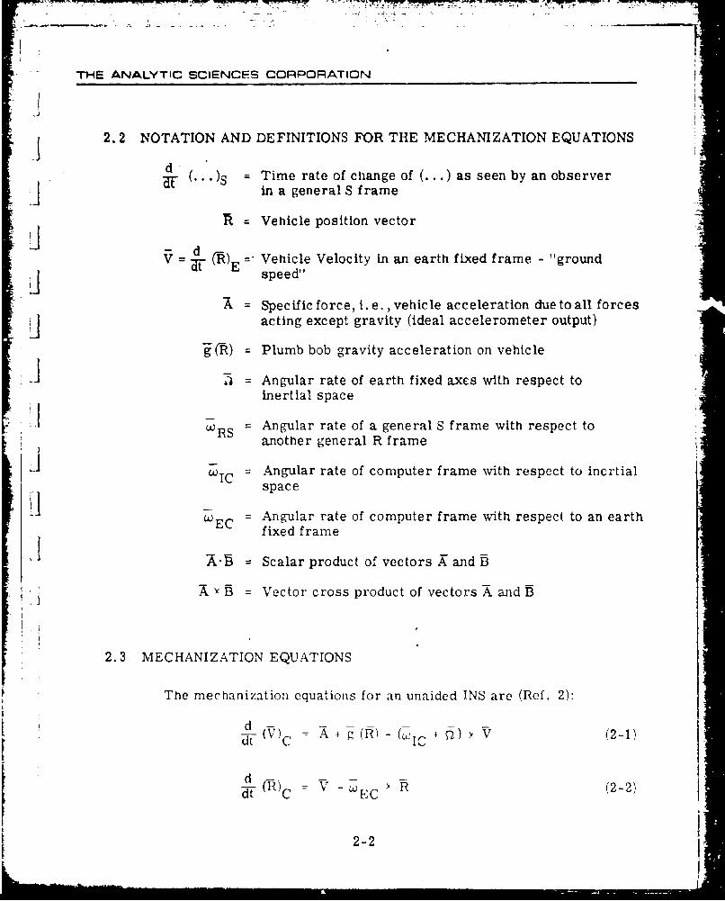
2.3 MECHANIZATION EQUATIONS

The mechanization equations for an unaided JNS are (Ref. 2):

(V)C A 4 g (R) - (CIC ) × V (2-1) -

d-C =MVR - >R (2-2)

2-2

THE ANALYTIC SCIENCES CORPORATION 4

Note that the vector quantities (ovorbar notation) in these equations require no

subscripts to designate a coordinate system since the magnitudes and direc-

tions they specify are independent of the reference frame in which they are

expressed. The vectors R, V, X, and g in Eqs. (2-1) and (2-2) are the "truo"i4position, velocity, specific force, and gravity acceleration. However, since

the navigation computer deals only with "computed" quantities (PC) VC, A

the equations actually 'mechanized are:

d (23"Ar•~c=:c+ •c•!(•c)÷c~ • • (2-3)

d R (2-4)-it (-) 'C W;EC -c

where

"�"A = accelerometer outputs

WC = INS outputs of vehicle groundspeed (a 3-vector)C

RFC = INS outputs of vehicle position (a 3-vector)

The term gC(RC) in Eq. (2-3) must include earth oblateness terms in order to

provide an accurate g'avity computation (Ref. 10). Neglecting the earth's

ellipticity can cause position errors on the order of ten nautical miles (Ref. 3).

Although the non-spherical character of the earth is explicitly expressed in the

mechanization equations, usual practice is to neglect it in the error equations.

Further discussion of Eqs. (2-3) and (2-4) is given in Appendix A.

2-3

I •I THE ANALYTIC SCIENCES CORPORATION

2.4 NOTATION AND DEFINITIONS FOR THE ERROR EQUATIONS

6,7 =7 - V(2-5a)

J 8 = - (2-5b)

i= C-jR (2-5c)j 1.=I

= small angle misalignment betwcen platform andcomputer frames (defined positive for rotation fromcomputer frame to platform frame)

= total accelerometer error (difference between idealand actual accelerometer output)

.1- = gravity anomaly and vertical deflections (gravitydisturbance vector)

g = nominal value of. gravity (scalar)

C- = total gyro drift rate error due to all gyro error sourcesA

Ro = nominal radius of the earth (scalar magnitude)

R - magnitude of

2.5 ERROR EQUATIONS

The free (unaided) inertial system error equations are derived in

Appendix A. They are:

d ..TF~ S ' x XA +6g -(wjS 0) X6V (2-6)

d6) = -V -•E x 8R (2-7)d 6)S 6V - ES x 6R (2-7)

d i -+ (2-8)

2-4

i{i

THE ANALYTIC SCIENCES CORPRATION

where it is noted that they are coordinatized in a general S frame.

The gravity error ýFg is given by ýRef. 3):

HgRo 3 gR;0_ Zg-- - + R. ) -R (2-9)

RR

Note that Eq. (2-9) contains no explicit treatment of earth ellipticity errors.

Such errors are of second order size and, as such, may be neglected.

For a slowly-moving vehicle, equations (2-6) to (2-9) contain undamped

oscillatory dynamics at both the Schuler (84 minute period) and earth (24 hour

period) rates. This dynamical behavior is encountered in all terrestrial iner-Htal navigation systems, regardless of the nominal platform orientation (local

level, space stable, strapdown, etc.) and may be seen by writing out Eqs. (2-6)

to (2-8) in a particular reference frame and taking eigenvalues. That such is

the case is not surprising when it is recalled that Eqs. (2-6) through (2-9) express

vector quantities in a generalized coordinate frame. The dynamics they describe

must be invariant with regard to the reference system in which they are cast.

Later in this report these equations will be written out term by term.

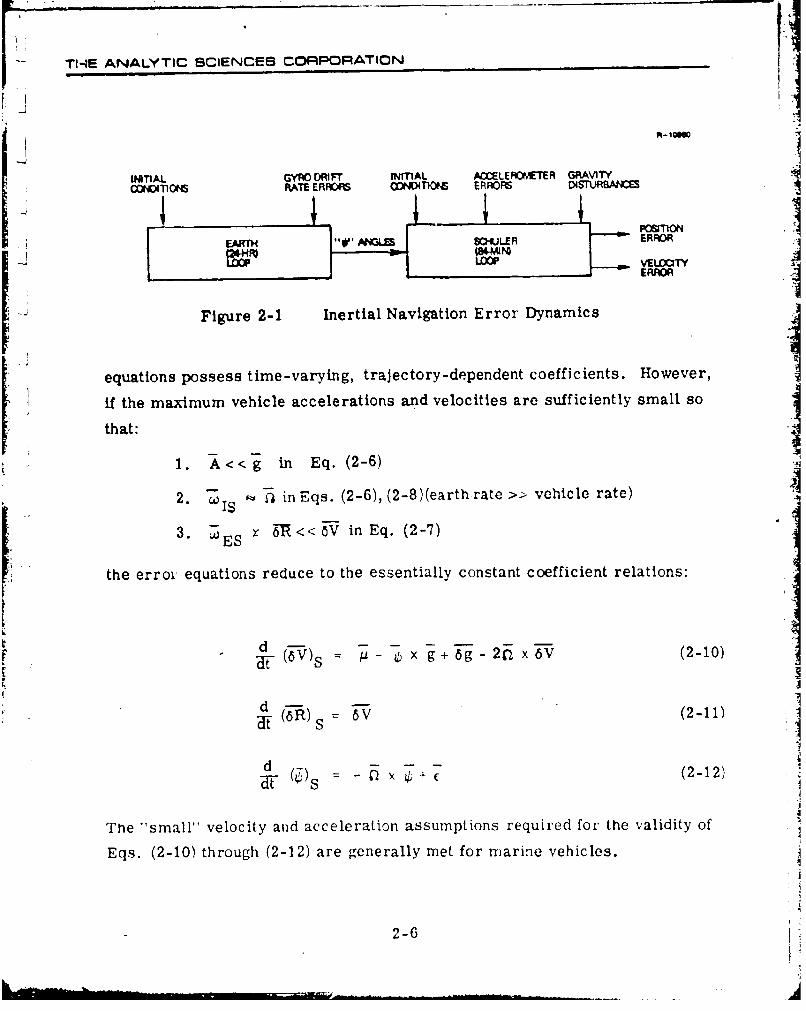
Note that the solution of Eq. (2-8) for the computer to platform mis-

alignments is independent of the position and velocity error equations (Eqs.

(2-6), (2-7)). The navigation error equations may thus be considered as being

driven by the T errors. This partial decoupling of the equations is depicted

in Fig. 2-1 and the attendant simplified form of the error equations is a major

rationale for expressing them in terms of the • angles.

It is appropriate to point out the difference in the character of Eqs.

(2-6) through (2-8) deperding upon whether the vehicle travels at "high" or"low" speeds. In general, for no limitations on rates of motion the error

2-5

T1-E ANALYTIC SCIENCES CORPORATION

COMN ATE 6RK; aCONIT ERARSf DtPTURBAMJCEPOSI ON

i - Figure 2-1 Inertial Navigation Error Dynamics

equations possess time-varying, trajectory-dependent coefficients. However,

if the maximum vehicle accelerations and velocities are sufficiently small so

that:

1. A <<g in Eq. (2-6)

2. W fJ in Eqs. (2-6), (2-8)(earth rate >> vehicle rate)

3 . W E S 6 <- <E6 V in E q . (2 -7 )

the errox equations reduce to the essentially constant coefficient relations:

S(GV)s = - x g + 6 g - 2r x 6 V (2-10)

6 R-) = V (2-11)

)S -Q (2-12)

The "small" velocity and acceleration assumptions required for the validity of

Eqs. (2-10) through (2-12) are generally met for marine vehicles.

2-6


2.6 PLATFORM MISALIGNMENT EQUATIONS

The angular misalignment between the true (5) frame and the com-

jputer (C) frame is defined as the small angle "6 where positive "6 is taken from

the true frame to the computer frame. This angle is a function of position

_J error only.

8j = 6 (2-13)

The small angular misalignment, T, between the platform frame and

•j the true frame (platform "tilt") is given by:

I ¢ =• + •(2-14)

where positive F corresponds to rotation from the true frame to the platform

j frame. Note that the solution of Eq. (2-14) for the vector angle ¢ provides the

azimuth error although the required combination of T components needed is

reference frame dependent.

It is not necessary to solve Eqs. (2-6) through (2-9) prior to finding

Sin Eq. (2-14). Instead, the expressions (2-13), (2-14) can be substituted

into Eqs. (2-6) to (2-8) and the error equation set expressed in terms of the

platform misalignment angles, T, instead of the computer misalignment, •.

I However this has not been done here for several reasons:j

1. The decoupling associated with the - angle representation(see discussion in previous Section) does not occur whenSis the misalignment variable in the equations.

2. The additional relations between 6 and 6f1 (Eq. (2-13)) must beincluded necessitating the specification of a reference frame inwhich the error equations are to be written. A resultant lossof generality occurs.

3. The 0 form is directly suitable for use with externally sup-plied stellar observation information. (- is the angle whichis measured by a star sensor.)

2-7

••" •" hi • -- " • •'' • •j

-- - - -- .----- ~ --~ A THE ANALYTIC SCIENCES CORPORATION

In the interest of completeness the 0 formulation of the error equations is givenjin Appendix B.

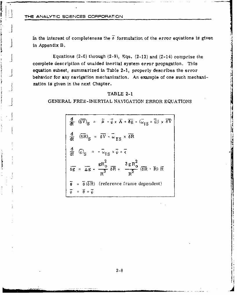
Equations (2-6) through (2-9), Eqs. (2-13) and (2-14) comprise the Icomplete description of unaided inertial system error propagation. Thisequation subset, summarized in Table 2-1, properly describes the errorbehavior for any navigation mechanization. An example of one such mechani-zation is given in the next Chapter.

TABLE 2-1

GENERAL FREE-INERTIAL NAVIGATION ERROR EQUATIONS

d(~

d (6R)S = V -ES x 6R

d - -"

I: 2 2g gR2 3gR 2

6g g= &g- u-7a-6R+ --- 5- .6RR R

e (6R) (reference frame dependent)

2=-8

2-8V

3. SPECIALIZATION OF THE ERROR EQUATIONS TO A WANDER- NAZIMUTH LOCAL-LEVEL INERTIAL SYSTEM MECHANIZATION

Some inertial systems are designed to mechanize the

navigation equations in a local-level, wander-azimuth

K configuration. Accordingly, in order to be directlyJ

applicable to analysis involving such systems, the

<ii jgeneralized error propagation equations listed in the

previous Chapter will now be detailed in this mechaniza-

tion.

3.1 DESCRIPTION OF WANDER-AZIMUTH, LOCAL-LEVEL MECHANIZATION

A wander-azimuth, local level mechanization involves

-I aligning the INS platform to be perpendicular to the

local geodetic vertical. The gyro which senses rotation

about the vertical is untorqued* and, as a result, the

platform will not maintain a particular terrestrial head-

* I ing reference. Instead, orientation with respect to

north will vary with time and vehicle position by the

so-called "wander angle." The geometry is depicted in

Fig. 3-1.

* The vertical gyro is untorqued only insofar as navi-gation variables are concerned. Torques applied tocancel bias error or to align the platform are leftunaffected by this disucssion.

3-1

i )


j~- L• -I

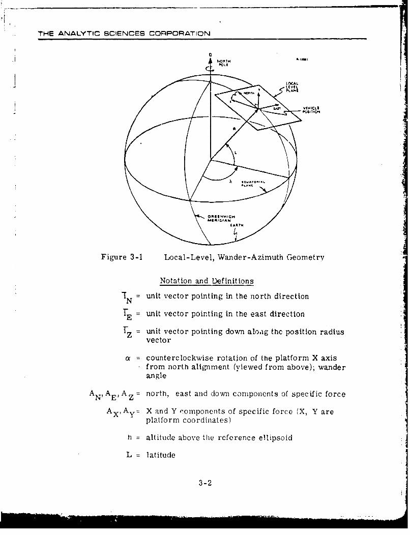
Figure 3-1 Loceal-Level, Wander-Azimuth Geometry

Notation and Definitions

IN = unit vector pointing in the north direction

t= unit vector pointing in the east directionE

Z = unit vector pointing down aloag the position radiusvector

S= counterclockw ise rotation of the platform X axisfrom north alignment (viewed from above); wanderangle

A N' AE AZ= north, east and down components of specific force

AXA = X and Y components of specific force (X, Y areplatform coordinates)

h = altitude above the reference ellipsoid

L = latitude

3-2

" rHE ANALYTIC SCIENCES CORPORATION

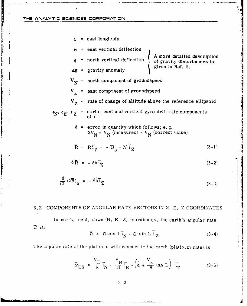
x = east longitude

,• = east vertical deflection[ A more detailed description

t = north vertical deflection of gravity disturbances is

Ag = gravity anomaly given in Ref. 5.

"VN = north component of groundspeed

VE = east component of groundspeedr V = rate of change of altitude aLove the reference ellipsoid

""N' (E' 'Z = north, east and vertical gyro drift rate componentsof T

6 = error in quantity which follows; e. g.F6 VN VN (measured) - VN (correct value)

R = RT -(R0 + h)1-z (3-I1 -)

6R = 6h- Z (3-2)

d (6 ) 6s--hZS z (3-3)

3.2 COMPONENTS OF ANGULAR RATE VECTORS IN N, E, Z COORDINATES

In north, east, down (N, E, Z) coordinates, the earth's angular rate

37 is:= cos I,TN -N sin L i'z (3-4)

The angular rate of the platform with respect to the earth (platform rate) is:

VE N tan L i (3-5)

"ES - N RE R z

3-3

THE ANALYTIC SCIENCES CCOPORATION

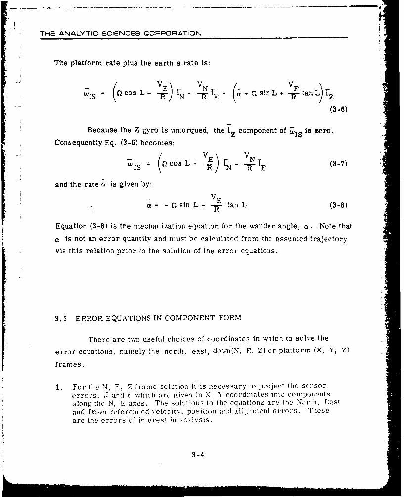
The platform rate plus the earth's rate is:

WIS = (Ccos L+ -E)N- VIE- + sin L+ V E tanL)z

(3-6)

Because the Z gyro is untorqued, the iz component of is is zero.

Consequently Eq. (3-6) becomes:

IN - E (3-7)

and the rate a is given by:

Va. •= -gasin L- E tan L (3-8)R

Equation (3-8) is the mechanization equation for the wander angle, a. Note that

a is not an error quantity and must be calculated from the assumed trajectory

via this relation prior to the solution of the error equations.

3.3 ERROR EQUATIONS IN COMPONENT FORM

There are two useful choices of coordinates in which to solve the

error equations, namely the north, east, down(N, E, Z) or platform (X, Y, Z)

frames.

1. For the N, E, Z frame solution it is necessary to project the sensorerrors, j and c which are given in X, Y coordinates into componentsalong the N, E axes. The solutions to the equations are the North, E.astand Down referen(ed velocity, position and aliýmm'ent errors. Theseare the errors of interest in analysis.

3-4

THE ANALYTIC SCIENCES COIPORATION

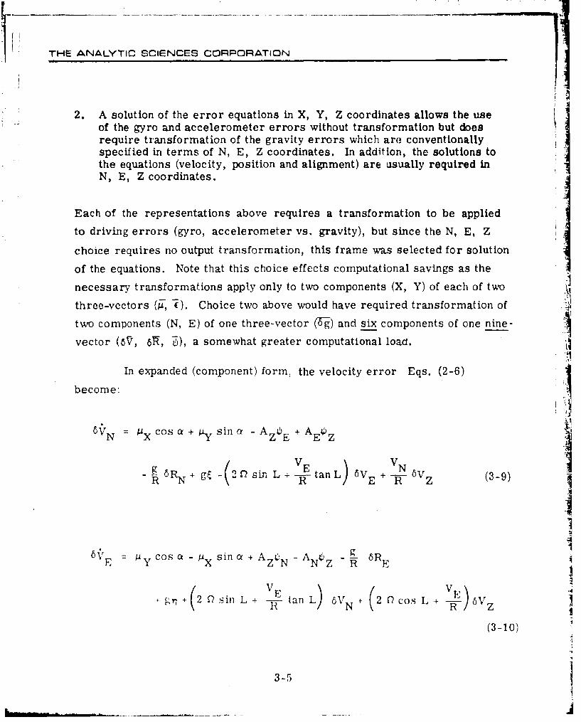
2. A solution of the error equations in X, Y, Z coordinates allows the useof the gyro and accelerometer errors without transformation but doesrequire transformation of the gravity errors which are conventionallyspecified in terms of N, E, Z coordinates. In addition, the solutions tothe equations (velocity, position and alignment) are usually required inN, E, Z coordinates.

Each of the representations above requires a transformation to be applied

to driving errors (gyro, accelerometer vs. gravity), but since the N, E, Z

choice requires no output transformation, this frame was selected for solution

of the equations. Note that this choice effects computational savings as the

necessary transformations apply only to two components (X, Y) of each of two

three-vectors E, ). Choice two above would have required transformation of

two components (N, E) of one three-vector (T-) and six components of one nine-

vector (6V, 617, ý), a somewhat greater computational load.

In expanded (component) form, the velocity error Eqs. (2-6)

become:

5VN /.x cosa + 4y since -AZEE + AE•Z 6v

-g 6RN-4 g- 2 sin L+EtanL )V +N 6V (3-9)

PC a n+A 6 -A 4 1 6RE Ay cosc -ZXsi ZN N Z R E

4g? 7 4\2 0 sin L + R tan L 6 N + R cosL + 6VZ

(3-10)

3-5

AE ANALYTIC SCIENCES CORPORATION

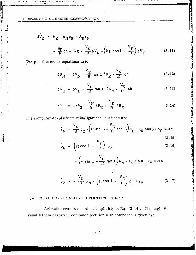
-8 ýZ +ANOE - AE N

2g Ag. N6VN 20cosL E 6V (3-11)+ ~- 6 N E

The position error equations are:

VE VN6 R E tan L 6 RE N 6h (3-12)

VE VEtEanVE + 6R -6- h (3-13)

-J VN VEE

S8h = -Sz+-R- R R (3-14)

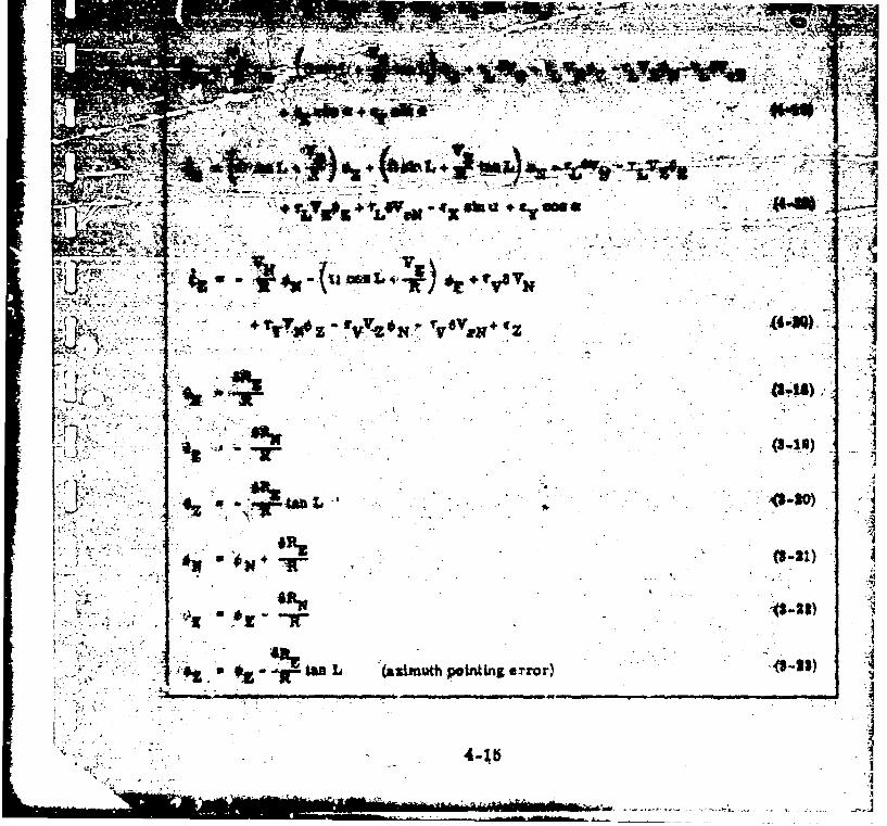
The computer-to-platform misalignment equations are:

SN =R• 'Z- 0 sin L + tan L) E

(3-15)

;bE= (C2osL+ R ) 0z (3-16)

+ 0sinL +--E tanL • xN•xsin a+Ey cosa

VN V0z - ER N + cosL+ R>E+ Z (3-17)

3.4 RECOVERY OF AZIMUTH POINTING ERROR

Azimuth error is contained implicitly in Eq. (2-14). The angle "6

results from errors in computed position with components given by:

3-6


I J 8R•eN-W(3-18) r:

0 E -~(3 -19)

; •- The components of the platform misalignment angle, ¢, are: -

O N (3-2R)

E = CELN+ R (3-2N)

6RE

ez FZ R tan L (3-23)

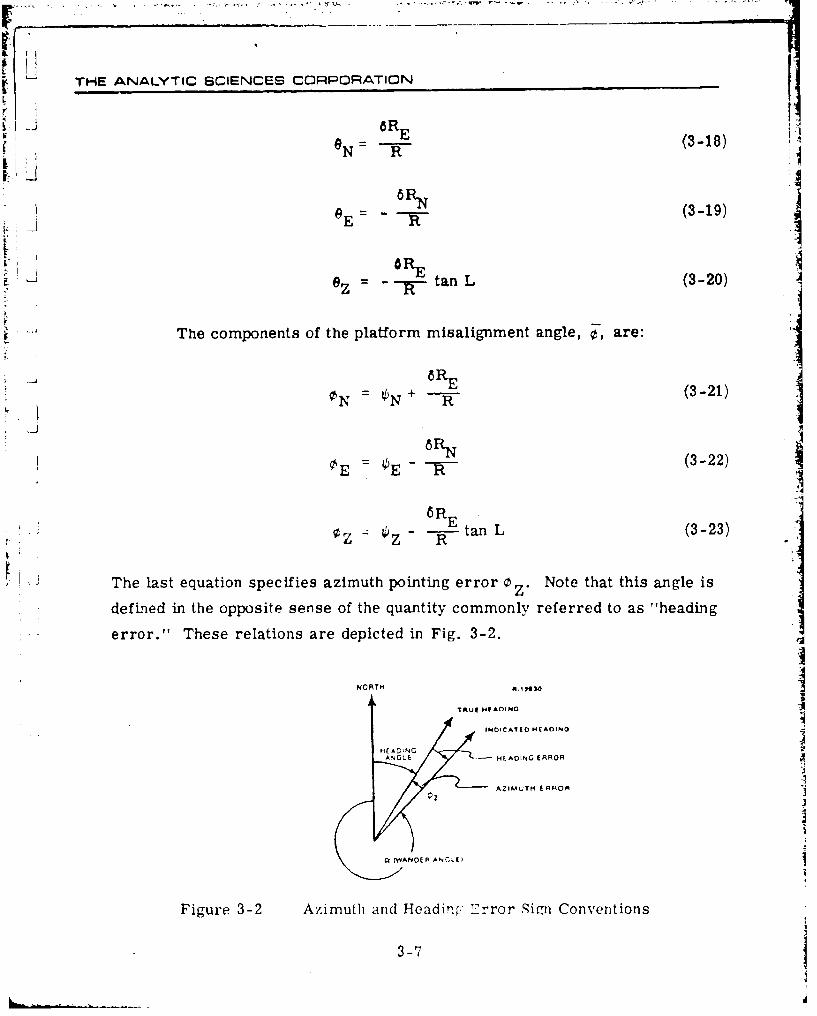
The last equation specifies azimuth pointing error lZ" Note that this angle is

defined in the opposite sense of the quantity commonly referred to as "heading •

error." These relations are depicted in Fig. 3-2. .

NOT.6R

IPIlOuCATEO ~AOINO

A~GLH - NADING E .RROR

• AZiMuTM rARDO I

0c rWANOEA ANCIkij

Figure 3-2 Azimuth and Headi(- r C n

3 -(3 2

TH-E ANALYTIC SCIENCES CORPORATION

Equations (3-9) through (3-20) and Eq. (3-23) comprise the subset

which describes error propagation in an unaided local-level, free-azimuth

inertial navigator. Equations (3-21, 22) are auxilliary relations which may be

tused to find platform tilt errors.

3-8

."---' , • -~---, = :". .- .. .. S " " • . .• _- ' -,'• " -" .- .. •' T


4. INERTIAL SYSTEM MECHANIZATION AND ERROR EQUATIGNS

WITH STABILIZED ALTITUDE CHANNEL, ALTITUDE

DAMPING AND VELOCITY DAMPING

4.1 RATIONALE FOR DAMPING

It is well known that the altitude channel of an unaided inertial system

is unstable (Ref. 2). This characteristic is commonly corrected by employing

an externally measured altitude reference (e.g., barometric or radar altimeter)

to stabilize the INS vertical axis. A detailed discussion of altitude damping is

given in Ref. 6.

The horizontal channels of an unaided INS, while not unstable, are

undamped and hence only marginally stable. A small amount of spectral energy

from error sources which drive the Schuler-loop (accelerometer noise, vertical

deflections, earth loop errors (0) etc.) is sufficient to cause unbounded growth

of the navigation errors. These errors are "damped" by making use of exter-

nal velocity measurements such as are furnished by doppler radar.

In the discussion above, a distinction between "vertical" and "horizon-

tal' channels has been made largely to take advantage of intuitive notions which

are typically directed toward local-level mechanization schemes. In general,

as i-. illustrated hi the equations below, externally supplied altitude and velocity

information may be used to stabilize and damp an INS regardless of its mechani-

zation (local level, space stable, strapdown, etc.).

4.2 NOTATION AND DEFINITIONS F'OR MECHANIZATION AND ERýROREQUATIONS

h = Vehicle altitude supplied by external altitude reference

4-1

LJ THE ANALYTIC SCIENCES CORPORATION

V = Vehicle groundspeed supplied by external velocitylr reference

V = Velocity damping state variables (a 3-vector)d

i K = First order damping constant matrix1

K 2 = Second order damping constant matrix

r = Gyro torquing feedback gain matrix (earth ratej gyrocompassing constant)

g(R c, inr ) = Plumb bob gravity acceleration calculated from

both externally and inertially indicated altitude

K = Weighting constant (scalar) governing the pro-portion of externally and inertially measuredaltitude used to calculate gravity

6 V r External velocity reference errorS~r

6 V d = Velocity damping state error

4.3 GENERAL MECHANIZATION

4.3.1 Schuler Loop Damping Mechanization

The specific force equation (2-3), modified to include continuous

second-order external-velocity damping and altitude stabilization is given belowI. dt- (V)C = AC + g (RC'"r)" (WIC+ Cl) x VC K1(V C-Vrr)+ K2 Vd (4-1)

with the auxiliary relation:

dId )C CK (VC V 2r K2Vd (4-2)

Note that for an error-free system, the reference velocity, V isr

equal to the computed velocity, VC, and the initial condition of the second order

4-2


damping variable, Vd, is zero. Also, in such an ideal system 1C, and hr

provide the same value of gravity. Under these conditions Eq. (4-1) reduces

to Eq. (2-3) hence demonstrating the dynamic exactness of the aided system.

Equations (4-1) and (4-2) describe a second-order velocity-damped INS mechan-

ization. This consists of proportional and integral feedback of the difference

between externally and inertiallly measured velocity to the acceleration sum-

ming node. First orler velocity damping which involves only proportional

feedback may also be described by Eq. (4-1) by the setting of the gain constant,

K2 , to zero. The damping state variable, Vd and Eq. (4-2) become redundant

in this case.

4.3.2 Earth Loop Damping Mechanization

While a complete discussion of the various platform alignment proce-

dures is beyond the scope of this equation subset, error equation generality

requires consideration of platform misalignment angle recovery from the ex-

ternally supplied velocity data. For this purpose it is assumed that the gyros

are torqued with a signal which is proportional to the difference between iner-

tially-derived and externally-measured velocity, i.e.,

Total Command Gyro Rate = Mechanization Torqued Rate + r (V0 - Vr)

Note that the first term on the right hand side'of the expression above is the

commanded gyro rate corresponding to the particular mechanization involved;

hence it is generally different for each mechanization. The underlined term is

the additional gyro rate which incorporates the velocity feedback. As will be

seen in the next section, this term mechaniizes the earth loop damping.In considering this procedure, it is necessary to distinguish between the INS"navigate mode" and "alignment mode." The latter case in which ravigation

4-3

-. THE ANALYTIC SCIENCES CORPORATION

information is not being extracted from the INS but in fact is being supplied to

j it for purposes of systcm alignment is not considered here. Attention is con-

fined the navigate mode during which the system continuously supplies the

user with current values of his velocity, position and heading. One may look

at this velocity-to-gyro feedback in two ways, either as an alignment proce-

dure in which the navigate mode is maintained or as simply another use of

external velocity data' to improve knowledge of an INS variable, in this case •.

Mechanization considerations pertinent to the use of an external velocity sig-

nal to drive the gyros are:

- The external velocity reference must be very accurate inorder to prevent significant velocity errors from beingintroduced into the earth rate (l) loop.

S* Even a "good" external velocity reference will containenough error to require small values for the feedbackgain constants ("light" damping).

4.4 GENERALIZED ERROR EQUATIONS

4.4.1 Damped Schuler Loop Error Propagation

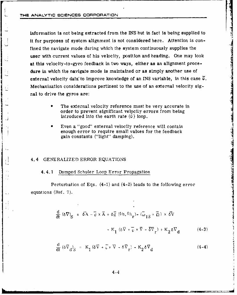
Perturbation of Eqs. (4-1) and (4-2) leads to the following error

equations (Ref. 7).

d(SV) CA -t.i x A + 6g (6h, 6 h r)- (Wis 0) x 6V

-K 1 (6V•+ x- )K 2 6Vd (4-3)

r 2 dd -d- (,5Vd)S K1 (6V + V 6V) - K2 6V (4-4)

4-4

THE ANALYTIC SCIENCES CIOUPORATION

In the derivation it is assumed that the externally-measured velocity is

available in platform-frame coordinates. (This is the usual case for aircraft

doppler or shipboard velocity log measurements.) The fact that the platform

and computer frames are misaligned by the angle • gives rise to the x x V

terms in Eq,. (4-3) and (4-4).

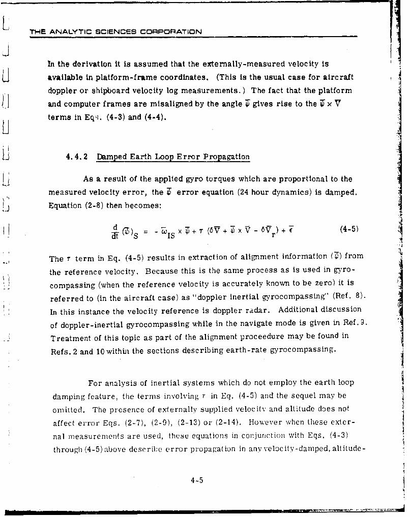
4.4. 2 Damped Earth Loop Error Propagation

As a result of the applied gyro torques which are proportional to the

measured velocity error, the T error equation (24 hour dynamics) is damped.

Equation (2-8) then becomes:

d r (4-it )S="aISi × r(V •V "r)+ 4

The r term in Eq. (4-5) results in extraction of alignment information (T) from

the reference velocity. Because this is the same process as is used in gyro-

compassing (when the reference velocity is accurately known to be zero) it is

referred to (in the aircraft case) as "doppler inertial gyrocompassing" (Ref. 8).

In this instance the velocity reference is doppler radar. Additional discussion

of doppler-inertial gyrocompassing while in the navigate mode is given in Ref. 9.

Treatment of this topic as part of the alignment proceedure may be found in

Refs. 2 and 10 within the sections describing earth-rate gyrocompassing.

For analysis of inertial systems which do not employ the earth loop

damping feature, the terms involving T in Eq. (4-5) and the sequel may be

omitted. The presence of externally supplied velocity and altitude does not

affect error Eqs. (2-7), (2-9), (2-13) or (2-14). However when these exter-

nal measurements are used, these equations in conjunction with Eqs. (4-3)

through (4-5) above describe error propagation in any velocity-damped, altitude-

4-5


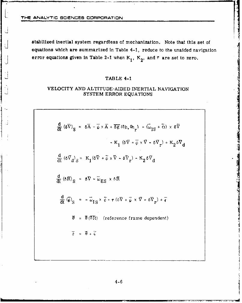
IIij stabilized inertial system regardless of mechanization. Note that this set of

equations which are summarized in Table 4-1, reduce to the unaided navigation

error equations given in Table 2-1 when KI, K 2, and 'r are set to zero.

TABLE 4-1

VELOCITY AND ALTITUDE-AIDED INERTIAL NAVIGATIONSYSTEM ERROR EQUATIONS

(T = 0A -0xA + 9-(6h, hr +) x

d = K1 (6 + x V -V) - K2 6 Vddf ('Vd'S Ir 2d

BT (•-s "ES

da(x -,r ISX + X v- 6V ) +

R "(5-R) (reference frame dependent)

L+1=4-6

4-6

UJ THE ANALYTIC SCIENCES CORPORATION

I

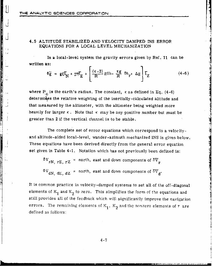
4.5 ALTITUDE STABILIZED AND VELOCITY DAMPED INS ERROREQUATIONS FOR A LOCAL LEVEL MECHANIZATION

In a local-level system the gravity errors given by Ref. 11 can be: written as:

6 t + +g g 6hr + g6h (4-6)-_ 'N E R ÷

where P 0 is the earth's radius. The constant, K as defined in Eq. (4-6)

determikes the relative weighting of the inertially -calculated altitude and

that measured by the altimeter, with the altimeter being weighted more

heavily for larger K . Note that K may be any positive number but must be

greater than 2 if the vertical channel is to be stable.

The complete set of error equations which correspond to a velocity-

and altitude-aided local-level, wander-azimuth mechanized INS is given below.* These equations have been derived directly from the general error equation

set given in Table 4-1. Notation which has not previously been defined is:

8VrN, rE, rZ = north, east and down components of 'V r

6 VdN dE, dZ north, east and down components of 3Vd.

It is common practice in velocity-damped systems to set all of the off-diagonal

elements of K 1 and K2 to zero. This simplifies the form of the equations and

still provides all of the feedback which will significantly improve the navigation

errors. The remaining elements of K1 , K2 and the nonzero elements of r are

defined as follows:

4-7

{. THE ANALYTIC SCIENCES CCRPORATION

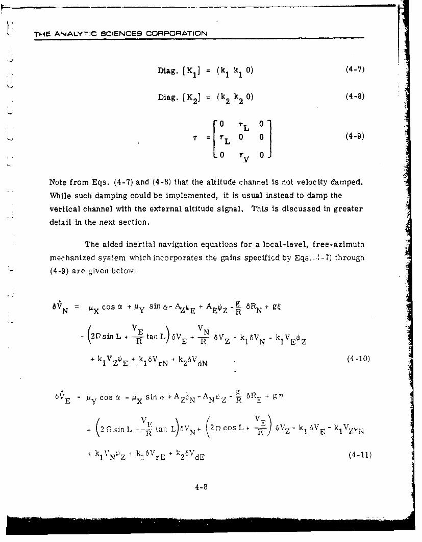
Diag. [K 1] - (kI k, 0) (4-7)

Diag. [K 2] (k 2 k2 0) (4-8)

[0 'rLT -[L 0 0 (4-9)

, 0 "V 01

Note from Eqs. (4-7) and (4-8) that the altitude channel is not velocity damped.

While such damping could be implemented, it is usual instead to damp the

vertical channel with the external altitude signal. This is discussed in greater

detail in the next section.

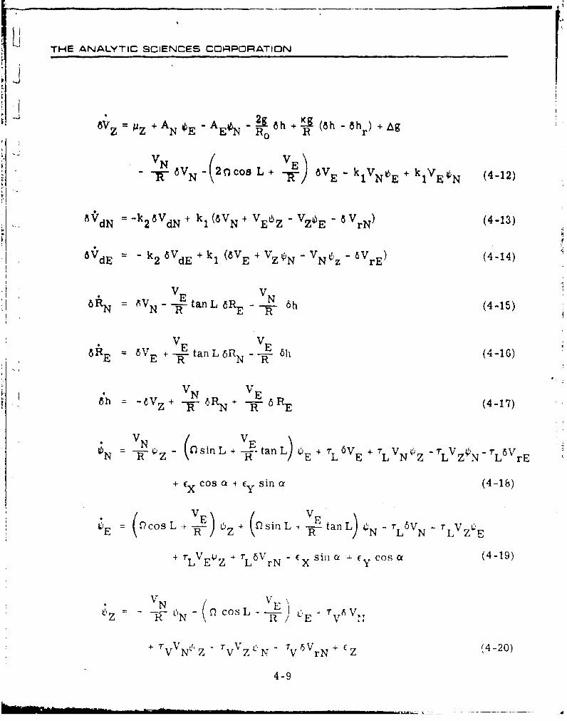
The aided inertial navigation equations for a local-level, free-azimuth

mechanized system which incorporates the gains specified by Eqs..1 -7) through

(4-9) are given below:

CosV0 + 4% sinl AWJ+ AEI 6 RN + gC

VN AXVAýE EZ

2DsinL +--E-tan L 6VE +-- 5V z N - kl6VN klVE~ 0

+ klV + kl6V k26V (4-10)IZ E 1 rN +2 dN

0V"E = cosa -P sinc +AzN-AN0! 6R E

+ (2n sinL- R tan L 6VN+ (2q cos L - Z- k, VE- klVZý.N

+ klVN Z - k.6Vr E + k 2 6VdE (4-11)

4-8

THE ANALYTIC SCIENCES COIPORATION

8Vz Z + AN EAEN 8 h + (8 h 8 h •)+g

Eo 1- -•

8 VN- Lo L+ 6 VE " klVN~bE + klVTE•N (4-12)

8VdN =-k 2 V6dN + kl (6VN + VECZ - VZOE - 8VrN) (4-13)

6 VrdE -k 2 6VdE +k1 (8VE +VzbN- VNz- 'VrE) (4-14)

6Z V VVNNtanL RE -6h (4-15)

N v

VE VE8k E 6= VE + g-tan L 6RN- Rh (4-1

VN VE-6 "Vz + -ý 6a R " 6 RE (4-17)

VN ( E= " - (0sinL+ -- tanL) ETrL6VOE +VN Z -LVZN-NrL'VrE

+ f Cos a + fy sin a (4-18)

xE OZy

=E (cosL - Z sinL + RtanL) N - TLSVN T LVz E

+ r ) L -ELVrN -+ X sila + (y- cos o (4-19)

VN V E)•' = R 0'N cos L +• T:' 6v V,,z N R E

+ •'vVN, z "Vv~z 1 N " TV 5V 6rN + (Z (4-20)

4-9


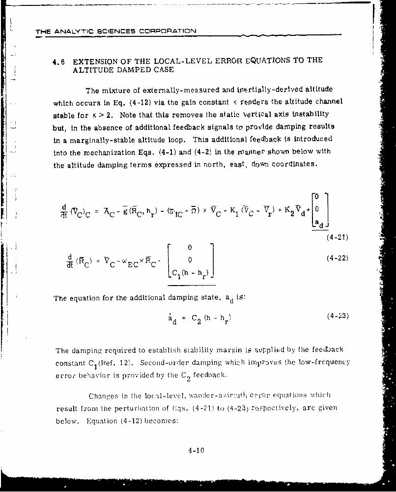
4.6 EXTENSION OF THE LOCAL-LEVEL ERROR EQUATIONS TO THEALTITUDE DAMPED CASE

The mixture of externally-measured and itirtially-derived altitude

which occurs in Eq. (4-12) via the gain constant K renders the altitude channel

stable for K > 2. Note that this removes the static vertical axis instability

but, in the absence of additional feedback signals to provide damping results

in a marginally-stable altitude loop. This additional feedback is introduced

into the mechanization Eqs. (4-1) and (4-2) in the nwpner shown below with

the altitude damping terms expressed in north, east, down coordinates.

rol-

d )C _C + g (RC' -+ +I<r r 2 d

dJ

(4-21)

d- 0 1d- (RC VC EC C 0 (4-22)

' C1(h - h r) _ -

The equation for the additional damping state ad is:

rad = C 2 (h - h (4 23)

The damping required to establish stability margin is .tqplied by the feecriack

constant C( (Pef. 12). Second-order damping which improves the low-frcquency -

error behavior is provided by the C2 feedback.

Changes in the lec a-level, wander-aziriuth eCror equationis which

result from the perturbation of Eqs. (4-21) to (4-23) rQ!5ect!vcly, arc given

below. Equation (4-12) becomes:

4-10


LIIýZ Z + -A L 6h+ g (6h - 6hr)&

•j 6Vz = .Z+ ANE-E -- --±•h ,+(4-24)

I VV- 6VN" 2 0cosL+ V,)6VEk1VNE+klVEN +k ad

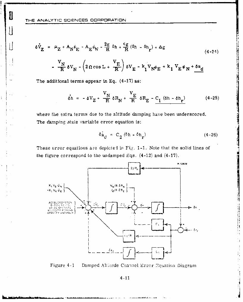
The additional terms appear in Eq. (4-17) as:

*VN VE

6 6h : VZ+ 6RN+ -w RECl(6h -6h) (4-25)

where the eixtra terms due to the altitude damping have been underscored.

The damping state variable error equation is:

6a C2 (6h - 6h) (4-26)

These error equations ace depicte-I ! Fig, 1-1. Note that the solid lines of

the figure correspond to the undamped Eqs. (4-12) and (4-17).

- 12829

AC~EL~F2E1E 1 R,

IV,AC, Oý:i,•!'E 5

GnAVcr Tv C4,,LY I .. AN L

--

Fig-ure 4-1 Damped Alý 0.0de Channel Errcr 7quatiori Diagram

4-11

"I-THE ANALYTIC SCIENCES CORPORATION

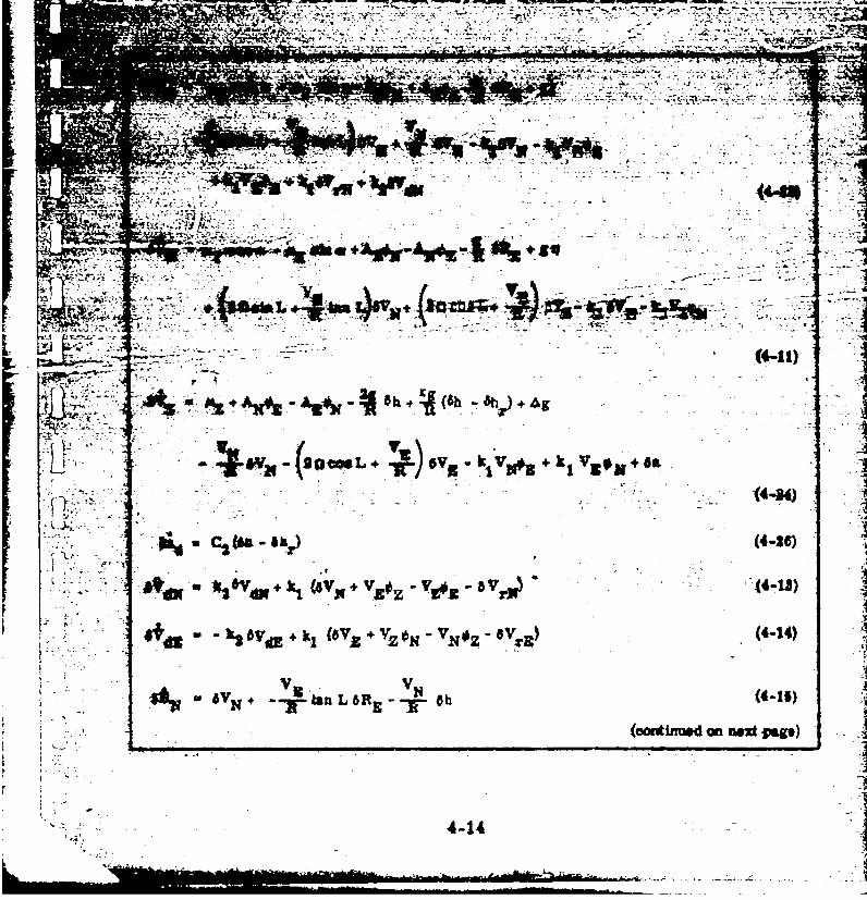
The complete set of error propagation relations for a velocity and altitude

aided local-level, wander-azimuth inertial system have now been set down. They

are given again in Table 4-2 for the convenience of the reader. Equation

numbers identify the portion of the text in which each equation is originally

stated. The following points are noted in regard to these equations.

* •The equations are valid for any combination of dampingconfigurations including zero damping; there are norestrictions on the values of K, kip k2 , rL, TV, C1 and C2 .

Thus analysis of a continuously damped INS may be per-formed for any permutation of the following external aidschemes:

External altitude measurementsExternal velocity measurementsFirst order damping (level and/or altitude channels)Second order damping (level and/or altitude channels)Navigation mode gyrocompassing

The equations may easily be assembled into "state spacei i form", namely

x = Fx + u (4-27)

which is the formulation most suited for covariance erroranalysis.

"" This set of equations also describes error behaviorin a north-slaved, locally-level INS if a is set tozero.

* The error equations of a continuously-damped iner-tial system have been shown to be the same for bothlocal-level and space-stable coordinate framemechanizations (Refs. 1, 13). While the gyro andaccelerometer error models differ for these twomechanizations, the dynamics of the error propa-gation are invariant if the damping is implementedin the same manner for both mechanizations. Con-sequently the local-level equations may be modifiedto be suitable for space-stable inertial platformanalysis.

4-12

L!.

THE ANALYTIC SCIENCES CORPORATIONI=

* The presence of the gyro torquing feedback terms In the0 equations (4-18 through 4-20) results in additionalL• terms which couple •hem with the velocity equations

(4-10 and 4-11). Hence damping of the 24 hour dynam-ics (C equations) links the earth-rate (24 hour) andSchuler (84 minute) loops.

* The Foucault oscillatory mode (approximately the fre-

"quency difference between the two level-axis Schuler-loop frequencies) which is manifest as amplitude modu-lation of the velocity and position errors is also dampedby the level channel velocity damping (kl). For a morecomplete discussion of Foucault mode decay character-istics see p. 148 ff of Ref. 2. The topic is also treated"in Refs. 3, 6, and 11.

* With the INS natural modes damped as described by theequations of Table 4-2, all errors except those risingfrom the polar component of gyro drift rate are bounded.

4-13i

I LI

1~41 W,.'

NOW

to #gk*L + %4 6V k-1~Ck V*+6

(4-21)

v v

4-14

-

-It~

l ' P - -

__ rr

/7 a w intn oina. eror

C-4-15

THE~ ANALYTIC SCIENCES CORPORATION#

APPENDIX A

A DERIVATION OF THE NAVIGATION ERROR EQUATIONS*

A derivation of the navigation error equations which follows directly

from the mechanization equations is briefly documented here. By this approach,

* :errors in ground speed and position error of the vehicle as seen in the true

frame are obtained directly. The philosophical approach is that of Ref. 2.

A. 1 THE MECHANIZATION EQUATIONS

The navigation mechanization equations derived in Ref. 2 are repro-

duced below-

P = A +g(l) - X V (A.1-1)

and

PS(R) PE (R) -0 ES x R

W- ES x R (A.1-2)

where

dPt ))S = the time rate of change of () as seen by anobserver in the S frame

dP ) = = )E time rate of change of () as seen in an earthfixed frame

gT = vehicle position vector

= PE (R) = vehicle velocity in an ea,'th fixed frame. i.e.,ground speed"

This Appendix has been extracted from Ref. 14.

A-i

U THE ANALYTIC BCIENCES CORPORATION

JI

7I = angular rate of earth fixed axes with respect to inertialspace

= angular rate of S frame w. r. t. inertial space

WES angular rate of S frame w. r.t. an earth fixed frame

=non gravitational force on vehicle (ideal accelerometeroutput)

9(') plumb bob gravity force on vehicle

The S (true) frame is the coordinate frame in which the solution to the

navigation mechanization equations is derived. Though usually chosen with

some good engineering justification, the S frame is not unique. The mechani-

zation equations can just as well be written in some other rotating frame, in

which case they would have the form:

P (V) = + A+-9IC +Ct)x (A. 1-3)

C I

and

P (R) =V-W X (A.1-4)C EC

In the sequel, "C" will denote the computer frame.

A.2 SOME COMMENTS ON ERROR ANALYSIS PHILOSOPHY1

In many error analyses only two coordinate systems are considered:

the S frame in which it is desired to mechanize the navigation error equations,

and the frame physically instrumented by the inertial platform. Though not

apparentsuch an approach can lead to incorrect definition of perturbation (i.e.,

error) quantities. These ambiguities are easily resolved by the introduction of

a third coordinate system, namely the computer frame. All errors are then

A-2

U THE ANALYTIC SCIENCES CORPORATION

defined with respect to this frame. The heuristic reasoning for this approach

-runs somewhat like this. At each point in time the computer may be viewed as

constructing a true coordinate frame at its computed position. It then determines

the angular rate of this coordinate system with respect to inertial space using

both its computed position and velocity. This is the computer frame of Eq.

(A. 1-3) and is a valid frame in which to solve the mechanization equations.

Indeed, this is exactly what happens. The computer integrates the mechaniza-

Stion equations in the frame defined by its output. Errors in this mechanization

arise from three sources: (1) acceleration has been measured in the platform

frame and not the computer frame, (2) gravity is incorrectly computed since

the computer frame is not coincident with true vehicle position, (3) computed

Svehicle velocity does not equal true vehicle velocity. The first error results

from angular misalignment of the platform and computer frames while the

second and third errors are caused by relative motion between the computer

and true frames.

At first glance, one may be disturbed that no error arises due to

incorrect computation of the computer frame angular rate, since such a term

always seems to be present when referring all errors to the true (S) frame.

But one must realize that the computer frame Is entirely defined by computed

position and velocity. There is no error in the state of this frame. If desired

it could be realized physically by constructing an S frame at the computed

position and rotating at the computed angular rate. Alternately, one may say

that the computer makes an error in computing the angular rate of the true (S)

frame. Thus the Coriolis correction applied to -+ g is (-wIC + 0) x V and not

(ccS i + U) x V. But this is precisely Eq. (A. 1-3) and the computer does indeed

generate PC().

A-3


A. 3 THE ERROR EQUATIONS

From the foregoing discussion the computer actually mechanizes

P ) = c+ (-Rc) (IC + 7) xVC (A. 3-1)

and

PC(RC C -. ,EC x RC (A.3-2)

where

¢ = computed vehicle ground speedC

SC= computed vehicle position

C = accelerometer outputs as interpreted by the computer

Let:

V -V +W'C-

= R c g + T (A. 3-3)

where the unsubscripted variables represent true quantities and the 6 termsrepresent as set undefined errors. Putting Eqs. (A.3-3) in (A.3-1) and

subtracting (A. 1-3) yields

p (&ýV) + b-6 +g- (W:-+ x '& V(A.3-4)

Likewise putting Eq. (A.3-3) in Eq. (A.3-2) and subtracting Eq. (A.1-4)

PC (6-R) = - U EC Y 6-• (A. 3-5)

In an error analysis the position and velocity of the true frame are

specified (this is equivalent to specifying the vehicle mission profile). Thus

W is and L:ES are prescribed. For this reason the differential equations

A-4


characterizing error propagation are best written in the "S" frame. The

j appropriate Coriolis conversions are:

PC(d )= PS(6-V) + WC x 6V (A.3-6)

and

P C (8 R= PS( 6 R) + w CS x 8R (A.3-7)

Equation (A. 3-6) in Eq. (A. 3-4) and Eq. (A. 3-7) in Eq. (A. 3-9) produces the

desired final relationships:

PS(+'V) = + ('WIS + D) x 6 (A.3-8)

and PaS (P5 R) = V - Z, ES x 6 (A. 3-9)

Equation (A.3-8) describes the time evolution of error in determining vehicle

velocity with respect to an earth-fixed frame while Eq. (A. 3-9) gives the time

evolution of the error in determining vehicle position.

Equations (A. 3-6) and (A. 3-9) can be obtained by an alternate and

instructive route. The development for Eq. (A.3-8) is presented here. Apply-

ing Coriolis' law to PC (Vc ) one obtains:

PC(V = PS((V C) + CS xVC (A.3-10)

Eq. (A. 3-10) in Eq. (A. 3-1) yields:

Ps(V + g(%s)-(• 1 I +i) C (A.3-11)

Subtracting Eq. (A.1-3) from Eq. (A. 3-11) then gives Eq. (A.3-8).

The errors 5A and 6 g must now be determined. Denoting the total

accelerometer error by 'g the accelerometer output is:

A-5

T THE ANALYTIC SCIENCES CORPORATION

N 0 = K+A-(A. 3-12)

,u may include random errors, scale factor errors, etc. The components of

Eq. (A. 3-12) which are available in platform axes are taken by the computer to

be the components of XK0 in the C frame. Thus the vector A° is rotated by the -icomputer through - , the small angle misalignment between computer and

platform axes to become:

C -X0 0 O Ae (.3-3

[It follows from Eq. (A. 3-3) that:

= ~xK (A. 3 -14)

H! Errors in determining g include errors in computing plumb bob gravity and the

computer's lack of knowledge of vertical deflections and gravity anomaly. At

worst the error in computing the centripedal term in g(R) is two orders of

magnitude less than that obtained in computing the mass attraction gravitational

force, gm" Denoting gravity anomaly and vertical deflections by 6g one may

then write:

= m + A-g (A. 3-15)

The derivation of &-gm is well developed in Ref. 2 and will not be repeated here.

Likewise, the differential equation governing the time evolution of the ý angle

is derived in Ref. 2. The complete set of error equations is then:

p S (TV) = 6A + 3 (-e (is + 17•) × 7v (A. 3-16)

P (M-) = '5 - -U x × (A. 3-17)S ES

PS(Q) is + (A.3-18)

A-6


where FA' and Gg are defined by Eqs. (A. 3-13) and (A. 3-14) and T is the total

vector gyro drift rate, including random effects, biases, and scale factor

torquing errors, and g and g2 effects.

A-7


APPENDIX B

NAVIGATION ERROR EQUATIONS EXPRESSED IN TERMS OFPLATFORM MISALIGNMENT ANGLES

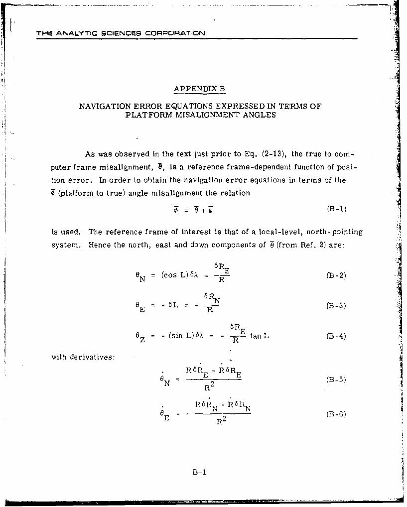
As was observed in the text just prior to Eq. (2-13), the true to com-

puter frame misalignment, •, is a reference frame-dependent function of posi-

tion error. In order to obtain the navigation error equations in terms of the

F (platform to true) angle misalignment the relation

+ (B-1)

is used. The reference frame of interest is that of a local-level, north-pointing

system. Hence the north, east and down components of e (from Ref. 2) are:

'REaN = (cos L)5X = R (B-2)

N RN

eE =-61L R R (B-3)

6 = -(sin L) , - R tanL (B-4)z R

with derivatives:• RSRE - R5RE0 RN RE 2 E (B-5)

N N

eE - 2 (B-6)

B-1

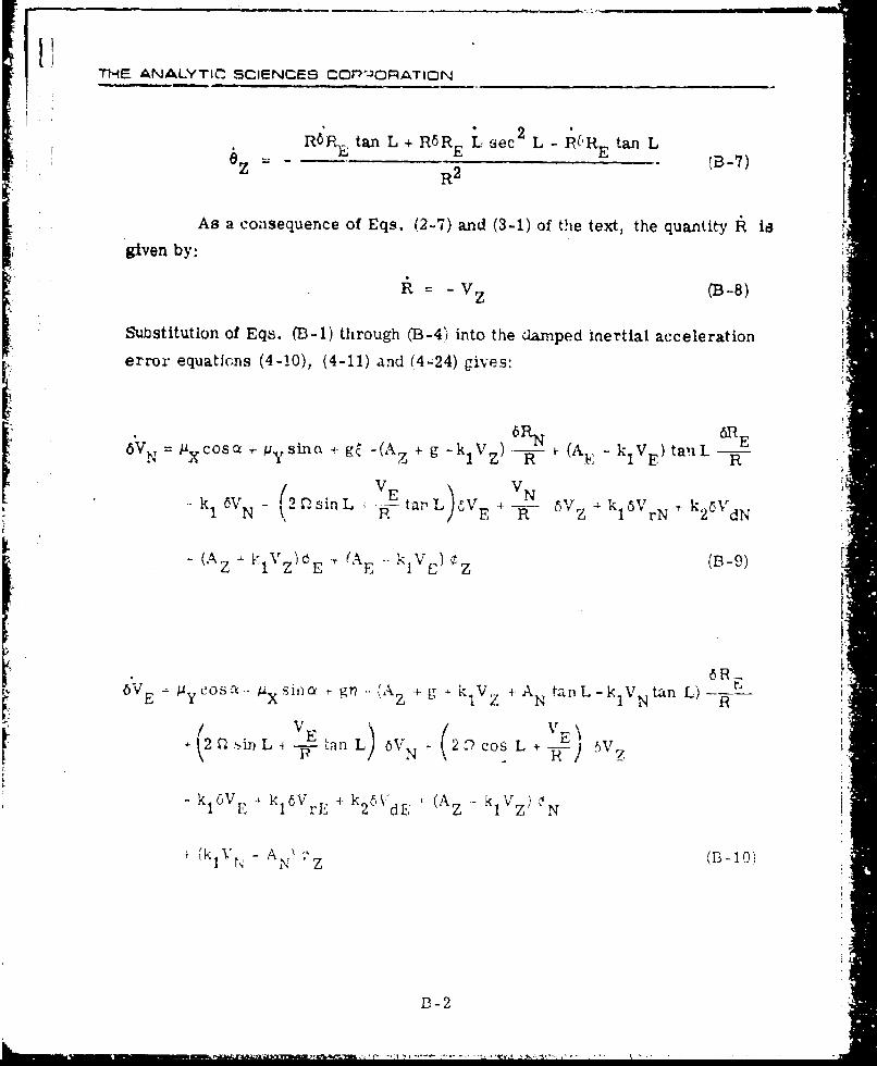
THE ANALYTIC SCIENCES COCP"-ATICN

Rý,,tn 6 £.iec L - R* REtan L B)E

ZzR2 i•

As a consequence of Eqs. (2-7) and (3-1) of the text, the quantity A is

given by:

R= -V (B -8)

Substitution of Eqs. (B-1) through (B-4) into the damped inertial acceleration

error equaticns (4-10), (4-11) and (4-24) gives:

6V RN 6RE •= 1XCOS + ySinc + g+ -(Az + g -kl1 )-Z--- + (A Y, - kIVE) tauL R

Vk 1 6VN - 2rsinL E Vtan L V + kNVN + k66Vd )

- (Az 1 ý lVz E (AE" kI V C) z (B1-9)

6"VE = yCOS .- 3 i xiia t g? (AZ g - kV'7 + AN tanL-klVN tan L)VE y ) _r1N

+ Qz sin L• i L-an L 6VN (2. • coS. L + •v :

- kiOVE 1 + k2 dE (Az 1kVz) CN

4(kV -A Z (B -10)

B- 2

I. THE ANALYTtC SCIENCES 00RPFPORATION

I-

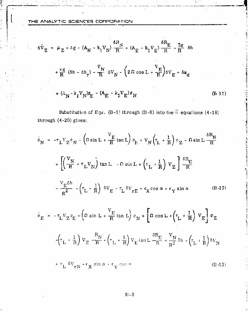
6RN 8RE 29'56 Vz i.z Z Lg (AN k IVN) -N - + (A E k IVE)R R

+ ý- (6h -h) - N - 2PcosL+ 6V + 6adR r NV{TI-) E 6

+ (AN - k - k-VE)N.)

Substitutkin of Eqi. (B-t through (B-8) into theý - equations (4-18)

through (4-20) gives:

VE 6 R N1TN I 'r rzCN= Dsin L + --- I-an L)OF;+ VN (T,+ n' -tsin L -N Z R

+ N -+ LVN ) tanL .P LvinL + (7L •. VZ ] 61

V E6h-+ L4 5VL - 61r(,L+Lr - xcosL ( +cysin t (B+-12)

ZE~ ~ E, RrN \L ,+• (0) sin L, +, ta 0CsL

E TLVE V N L L VEa (--S -Z

VLRV R+V+R' tan L 6RE N1 7-(LV 7 -'-R-- +f E+_ + Lý2 N

+ T L 6 VrN - X sin ac y cr (B3-13)

E-- 3

L THE ANALYTIC SCIENCES CORPORATION

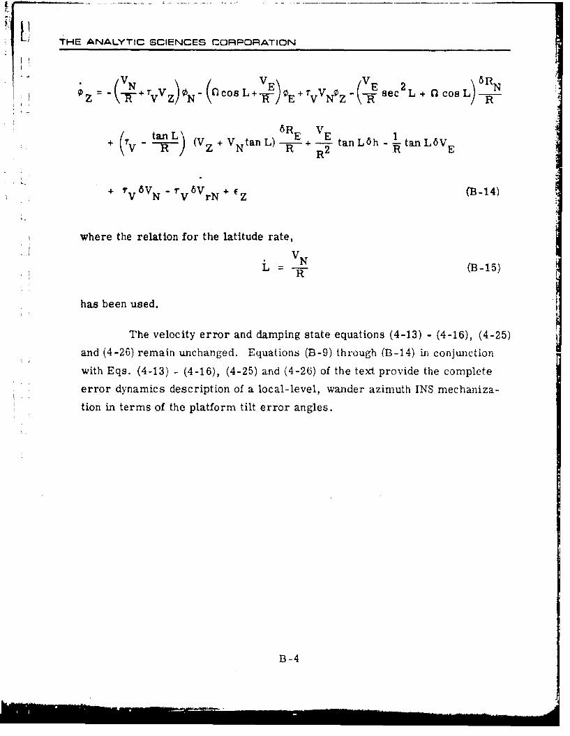
SNE\ /V 2 ~ RNZ= TF *rvVz ON - (cos L+- E LRfcosL R

t n- \(V+ + VNtan L) - + ÷ -tan L.6h tan L6VE

+ T'V 6VN " 6VrN + ' Z (B-14)

where the relation for the latitude rate,

N (B-15)i R

has been used.

The velocity error and damping state equations (4-13) - (4-16), (4-25)

and (4-26) remain unchanged. Equations (B-9) through (B-14) in conjunction

with Eqs. (4-13) - (4-16), (4-25) and (4-26) of the text provide the complete

error dynamics description of a local-level, wander azimuth INS mechaniza-

tion in terms of the platform tilt error angles.

B-4

F THE ANALYTIC SCIENCES CORPORATIC -1q

REFERENCES

1. Hutchinson, C. E. and Nash, R.A., Jr., "Comparison of ErrorPropagation in Local-Level and Space-Stable Inertial Systems,"IEEE Transactions on Aerospace and Electronic Systems, Vol. AES-7,No. 6, November 1971.

2. Pinson, J.C., Inertial Guidance for Cruise Vehicles, Chapter 4 ofGuidance and Control of Aerospace Vehicles, C.T. Leondes, editor,McGraw-Hill Book Co., 1963.

3. Pitman, G.R., Inertial Guidance, John Wiley and Sons, 1962 (pp. 163ff)

4. Deleted

5. Heiskanen, W.A. and Moritz, H., Physical Geodesy, W.H. Freemanand Co., 1966.

6. Nash, R.A. Jr. and Hutchinson, C.E., "Altitude Damping of SpaceStable Inertial Navigation Systems," IEEE Transactions on Aerospaceand Electronic Systems, Vol. AES-9, No. 1, January 1973.

7. See Reference 2 or 3.

8. Organizational Maintenance, Integrated Avionics Systems (for A7DAircraft), Oklahoma City Air Logistics Center (USAF), Technical IOrder 1A-7D-2-18, P. 5-9.

9. Doretzky, L. H. and Edwards, A., "Introduction to Doppler-InertialSystem Design," Journal of the American Rocket Society, December1959.

I10. Kayton, M. and Fried, W. R., Avionics Navigation Systems, John

Wiley and Sons, 19G9.

11. Britting, K. R., Inertial Naviation Svsteni Analysis, John %,'iley andSons, 1971, pp. 03 ff p. 113

R-1

I


12. D'Appolito, J.A. and Roy, K.J., "Integrated Navsat/Inertial Flight

Test Analysis", Chapt. 2, The Analytic Sciences Corp., Report No.AFAL-TR-74-56, April 1973.

13. Nash, R.A. Jr., Levine, S.A. and Roy, K.J., "Error Analysis ofSpace Stable Inertial Navigation Systems," IEEE Transactions onAerospace and Electronic Systems, Vol. AES-7, No. 4, July 1971.

14. D'Appolito, J.A., "The Evaluation of Kalman Filter Designs forMultisensor Integrated Navigation Systems," The Analytic SciencesCorp., Report No. AFAL-TR-70-271, January 1971.

Ri

Li

R-2

free-inertial and damped-inertial navigation mechanization and

Documents