introduction to digital data processing
TRANSCRIPT

International Institute of Seismology and Earthquake Engineering (IISEE) Seismology Course Lecture Notes
TRAINING COURSE IN SEISMOLOGY AND EARTHQUAKE ENGINEERING
Introduction to Digital Data Processing
Ver. 3.3.1 2010
by Toshiaki Yokoi
International Institute of Seismology and Earthquake Engineering (IISEE)
Japan International Cooperation Agency (JICA)

i
Contents
1. INTRODUCTION 1 1.1 Linear System 1
1.1.1 Signal, Input and Output 1 1.1.2 Linear System 2 1.1.3 Response Characteristics of Linear System 3
1.2 Digitization of Time-Dependent Functions 4 1.2.1 Dirac Comb Function 4 1.2.2 Time Series Discretization 5 1.2.3 Folding and Aliazing 5
2. FAST FOURIER TRANSFORM 8
2.1 Fourier Expansion of a Finite Time Series 8 2.2 Sinusoidal Functions and Fourier Spectra of Amplitude and Phase 9 2.3 Discrete Fourier Spectra 11 2.4 Algorithm for FFT 12
2.4.1 Removal of DC Component and Linear Trend 12 2.4.2 Tapering or Windowing 12 2.4.3 Zero Padding 13 2.4.4 Algorithm 14 2.4.5 Time Window and Periodicity 18 2.4.6 Spectral Smoothing 19
2.5 Practice for FFT 21 2.5.1 Cosine and Sine Wave 22 2.5.2 Constant 26 2.5.3 Impulse 27 2.5.4 Time Shift 28 2.5.5 Aliasing 30 2.5.6 Assumption of Periodicity 31
3. FILTERING TECHNIQUES 32
3.1 Weighted Moving Average 32 3.2 Convolution-Filtering in the Time Domain 34
3.2.1 Convolution 34 3.2.2 Filtering in the Time Domain by Convolution 34
3.3 Feature of Filter Wavelet 36 3.3.1 Phase 36 3.3.2 Frequency Components 40 3.3.3 Causality or Non-Causal Filtering 42
3.4 Recursive Filter 47 3.4.1 Laplace Transform 48 3.4.2 Filter Operation in the s-domain 48 3.4.3 Z-Transform 51 3.4.4 Filter Operator on the Z-domain 52 3.4.5 Analog Filters and their Transfer Functions 62 3.4.6 Excersize for Digital Filtering 68
3.5 Deconvolution or Inverse Filtering 71 3.6 Integration of Accelerograms or Base Line Correction 80
Fortran Programs 90 Reference for Further Reading 107

1
1. Introduction
In this lecture note, several basic and essential topics that are useful for understanding digital data processing techniques are explained. These topics are directly related to measurements using digital equipment.
1.1. Linear System Almost all measuring equipment is “linear systems.” This is because “linear systems” make it
easier to reproduce the measured value of the physical parameters from the results of the measurement.
1.1.1. Signal, Input, and Output Since it could be difficult to define the terms “signal”, “input” and “output” exactly, we
employ their practical definitions. A signal is any quantity that we measure or input. For example, mechanical signals may be
displacement, velocity, acceleration, or force, whereas electric signals may be charge, voltage, or current. Signals often depend on time. In seismology, we typically treat time-dependent signals. Such signals can have many relations. A system can be defined either as a relation between more than two signals itself, or an equipment (or algorithm) that yields such relations. The input can be defined as the conditions given to a system. The signal generated in the system that corresponds to the input is called the output (Fig. 1).
For example, consider ground motion. Ground motion will be the input to a seismograph (which is the “system”). The output is the recorded seismogram. If we consider a seismometer to be the system, the input will be the ground motion again while the voltage imbalance between the two terminals of the seismometer will be the output.
Fig. 1 Block diagram of a system.

2
1.1.2. Linear System Almost all the systems used in the measurement of physical quantities have “linear”
characteristics. This can imply the following. Suppose that the output of a system that corresponds to the input x1(t) is y1(t) while the output that corresponds to the input x2(t) is y2(t). The first requirement of a linear system is that the output corresponding to the input x1(t) + x2(t) is y1(t) + y2(t). The second is that the
output corresponding to αx1(t) is αy1(t), where α is a constant. These requirements lead to a proportional relation between the input and the output. Such a relation is called “linearity.” Namely,
If ( ) ( )( ) ( )⎩
⎨⎧
→→
tytxtytx
22
11 , then ( ) ( ) ( ) ( )
( ) ( )⎩⎨⎧
→+→+
tytxtytytxtx
11
2121
αα
Such “linear” characteristics of the relation between an input and an output ensure that the
input signal can be reconstructed by using the output signal. This is why almost all measuring equipment is linear systems. However, in reality, linear characteristics can be usually obtained only for a limited range of the input signal. Clipping of a seismometer and saturation of an amplifier are simple examples. When “linearity” is lost, the system becomes “non-linear” (Fig. 2).
There are several important “linear” transformations in mathematics that can be applied to physics, for example, the Fourier transform.
Fig. 2 Schematic figure showing both linearity and non-linearity.
INPUT
OUTPUT
O
LINEA
NON-LINEAR
NON-LINEAR

3
1.1.3. Response Characteristics of Linear Systems Suppose that g(t) is the output of a system when the input signal is a unit impulse δ(t). An
arbitrary function x(t) can be expressed by using the technique of “convolution” as follows.
( ) ( ) ( ) ( ) ( ) ( ) ( )∑∫∫∞
−∞=
∞
∞−
∞
∞−ΔΔ−
→Δ==−=
mumumtx
uduuu-txduutuxtx δδδ
0lim
.
The last term shows that x(t) is the weighted sum of the delta functions at an infinitively small Δu. Each delta function δ(mΔu) gives the output g(mΔu). The second requirement (mentioned previously in 1.1.2) suggests that the input x(t – mΔu)δ(mΔu) gives x(t – mΔu)g(mΔu), since x(t – mΔu) is a constant. The first requirement suggests that the input, that is, the sum of x(t – mΔu)δ(mΔu), gives the sum of the output for each weighted delta function x(t – mΔu)g(mΔu). Thus, the output signal that corresponds to the input signal x(t) is given by the following.
( ) ( ) ( ) ( ) ( ) ( ) ( ).0
limtyduutguxduugu-txumgum-tx
u m=−==ΔΔ
→Δ ∫∫∑∞
∞−
∞
∞−
∞
−∞=.
For a seismic signal, it is reasonable to suppose that g(t) = 0 at t < 0 ; then
( ) ( ) ( )y t x u g t u du = −∞
∫0.
These formulas show that the output that corresponds to an arbitrary input signal can be defined by g(t). In other words, the response to the unit impulse g(t) contains all information on the characteristics of a linear system. We call such a response “impulse response” or “system characteristics.”
Fig. 3 System response, input, and output signals.
SYSTEM
System Response Function R(t)
Input Time Series I(t) Output Time Series O(t)
O(t) = I(t)*R(t)

4
1.2. Digitization of Time-Dependent Functions Today, digital data acquisition and processing systems are so dominant in physical
measurements that we can expect analog or continuous systems to become obsolete by the first half of the twenty-first century. We can convert every analog signal to a digital once they are converted to the form of a voltage imbalance. Some basic knowledge is required to prevent difficulties that might occur during such analog-to-digital conversions, which are referred to as “discretization.”
1.2.1. Dirac Comb Function
First, let us understand the discretization process. Consider a box car function b(t):
( )b tB t t
t t=
≤>
⎧⎨⎩
, / ,, / .
0
0
20 2
The Fourier expansion in [–T/2, T/2] (T>t0) gives
( )b t
BtT
tt
t n Tn
nnn n( )
sin //
cos , /= +⎡
⎣⎢
⎤
⎦⎥ =
=
∞
∑0 0
01
1 22
22
ωω
ω ω π .
Note that the time window of the length T is used implicitly. T has to be longer than t0 and no other constraint is placed on it.
Let t0 tend to zero under the condition Bt0 = 1; in this manner, the Fourier expansion of δ(t) is obtained.
δ ω ω πω( ) cos , / .tT
tT
e n Tnn
i t
nn
n= +⎡
⎣⎢
⎤
⎦⎥ = =
=
∞
=−∞
∞
∑ ∑1 1 2 1 21
The Fourier expansion of the signal in a limited time window implicitly assumes the periodicity of the signal. This formula, when written in exact terms, represents an infinite series of the impulse and it is called as the Dirac comb function. Note that the interval between the delta functions is T.
Let us change the notation from T to Δt for the convenience of the following description (Fig. 4).
Fig. 4 Dirac comb function.
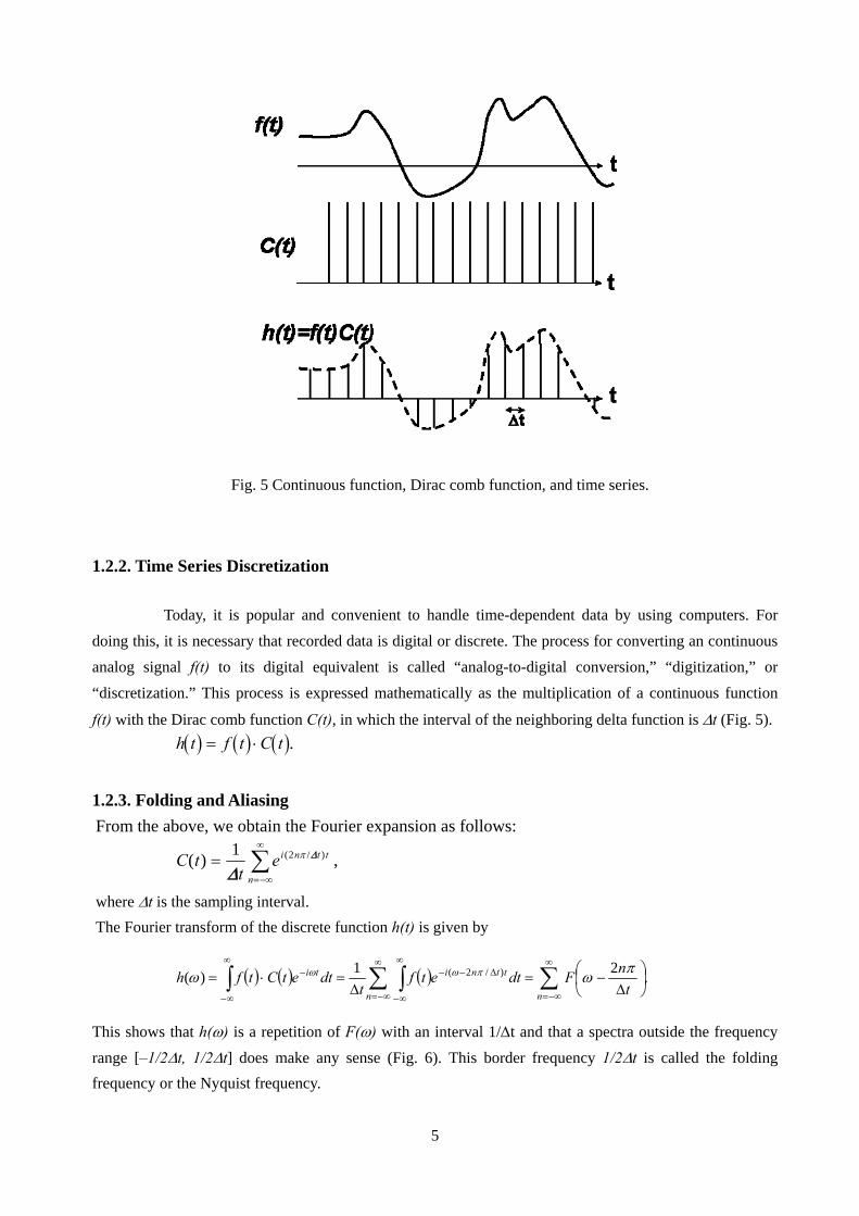
5
Fig. 5 Continuous function, Dirac comb function, and time series.
1.2.2. Time Series Discretization
Today, it is popular and convenient to handle time-dependent data by using computers. For doing this, it is necessary that recorded data is digital or discrete. The process for converting an continuous analog signal f(t) to its digital equivalent is called “analog-to-digital conversion,” “digitization,” or “discretization.” This process is expressed mathematically as the multiplication of a continuous function
f(t) with the Dirac comb function C(t), in which the interval of the neighboring delta function is Δt (Fig. 5). ( ) ( ) ( )h t f t C t= ⋅ .
1.2.3. Folding and Aliasing From the above, we obtain the Fourier expansion as follows:
C tt
ei n t t
n
( ) ,( / )==−∞
∞
∑1 2
ΔΔπ
where Δt is the sampling interval. The Fourier transform of the discrete function h(t) is given by
( ) ( ) ( ) .21)( )/2( ∑∑ ∫∫∞
−∞=
∞
−∞=
∞
∞−
Δ−−∞
∞−
− ⎟⎠⎞
⎜⎝⎛
Δ−=
Δ=⋅=
nn
ttniti
tnFdtetf
tdtetCtfh πωω πωω
This shows that h(ω) is a repetition of F(ω) with an interval 1/Δt and that a spectra outside the frequency range [–1/2Δt, 1/2Δt] does make any sense (Fig. 6). This border frequency 1/2Δt is called the folding frequency or the Nyquist frequency.

6
Fig. 6 Spectra of a time series.
The influence of digitization can be minimized easily when the Fourier spectra of the original continuous function have a negligible value at the Nyquist frequency. Otherwise, the foot of the
neighboring spectral peak invades in the range [–1/2Δt, 1/2Δt] and contaminates the signal. This phenomenon in the frequency domain is referred to as folding. The above consideration suggests that the
sampling interval Δt must be shorter than half of the shortest period that is included in the original continuous function. In other words, the frequency components of the period that is shorter than twice the sampling interval must be eliminated before digitization.
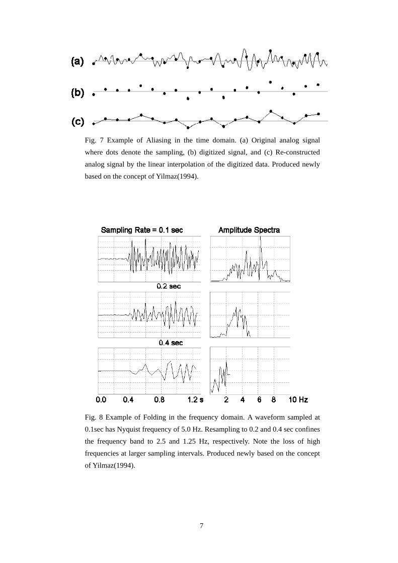
The disturbance is more clearly shown in the time domain. Fig. 7 clearly shows that coarse
discretization cannot identify fine peaks of the original continuous function, and the result is completely different from the original one.
Folding in the frequency domain and aliasing in the time domain represent the same
phenomenon. The relationship between aliasing and folding is schematically shown in Fig. 8.
An analog filter that is applied to the original analog signal in order to prevent the aliasing or folding is called an anti-alias filter. Re-sampling of the digital data also requires the application of an anti-alias filter.
7
Fig. 7 Example of Aliasing in the time domain. (a) Original analog signal where dots denote the sampling, (b) digitized signal, and (c) Re-constructed analog signal by the linear interpolation of the digitized data. Produced newly based on the concept of Yilmaz(1994).
Fig. 8 Example of Folding in the frequency domain. A waveform sampled at 0.1sec has Nyquist frequency of 5.0 Hz. Resampling to 0.2 and 0.4 sec confines the frequency band to 2.5 and 1.25 Hz, respectively. Note the loss of high frequencies at larger sampling intervals. Produced newly based on the concept of Yilmaz(1994).

8
2. Fast Fourier Transform (FFT) The Fourier transform is one of the basic mathematical tools used for data processing. A signal
in the time domain can be converted to one in the frequency domain by applying the Fourier transform and in this manner, different features of the converted data can be obtained. The Fourier transform of digital data is defined in this chapter.
There are several published subroutines of FFT in BASIC, FORTRAN, and C, which are very useful and simplify our task. However, we must focus on the definitions of the Fourier transform and its inverse transform that are given in different books. There are several possible definitions and mathematically they are all equivalent. When we use a subroutine given in a textbook, it is important to carefully read the main text. This lecture note employs the definition of Papoulis (1962, 1984) and Ohsaki (1976).
( ) ( )
( ) ( )⎪⎪⎩
⎪⎪⎨
⎧
⋅=
⋅=
∫
∫∞
∞−
∞
∞−
−
.21
,
ωωπ
ω
ω
ω
deXtx
dtetxX
ti
ti
2.1. Fourier Expansion of a Finite Time Series The Fourier expansion of a time series xm (m = –N/2 + 1,...–1, 0, 1, ...N/2) is given as follows.
The coefficient of expansion is given by
( ) .2,,1,0,1,,12,1 2/
12/
/2 NNkexN
CN
Nm
Nkmimk LL −+−== ∑
+−=
− π (1)
By using these coefficients, the original time series xm is expanded as
.2/,12/,2/
12/
/2 NNmeCxN
Nk
Nkmikm L+−== ∑
+−=
π (2)
Naturally, these formulas imply that any limited time series can be expanded into a finite number of sinusoidal waves of which the frequency is discrete, as shown in Fig. 9. Note that the periodicity in the time domain is implicitly introduced. Fig. 9 A series of sinusoidal curves with different frequencies, peak amplitudes, and phase lags can be superimposed to synthesize a waveform on the left-most curve as indicated by the asterisk. The sampling frequency of this waveform is 512Hz. The sinusoidal curves of frequencies higher than 33 Hz are omitted because their amplitudes are negligible. Produced newly based on the concept of Yilmaz(1994).

9
Fig. 10 Three sinusoids (left) and their amplitude (center) and phase spectra (right). The time between two consecutive peaks is the period of the sinusoid, the inverse of which is called frequency. Finally, the time delay of the onset is defined as phase lag. Produced newly based on the concept of Yilmaz(1994).
2.2. Sinusoidal Functions and Fourier Spectra of Amplitude and Phase Yilmaz(1994) shows a persuasive way of explaining Fourier Spectra of Amplitude and Phase. A
sinusoidal function is defined by its frequency, amplitude, and time shift, as shown by an example given in Fig. 10. A phase lag, that is, a time shift normalized by the period is usually used. Assume that the phase lag of the signals in the top panels is zero and its amplitude is unity. The frequency of signals in the top panels is 12.5 Hz. The middle panels have a half amplitude, frequency of 25.0 Hz and the phase lag is zero.
The bottom panels have unit amplitude, a frequency of 12.5 Hz, and phase lag of –π/2.
Every sinusoid drawn in Fig. 9 has a frequency, amplitude, and phase lag. The latter two
variables can be plotted against the frequency (Fig. 11). Each point along the amplitude spectrum curve (Fig. 11 Top) corresponds to the peak amplitude of the sinusoid at that frequency, as shown in Fig. 9. Note the correspondence of the peak in the amplitude spectra with the high-amplitude frequency range in Fig. 9. Each point along the phase spectrum (Fig. 11 Bottom right) corresponds to the phase delay of a peak or trough along the sinusoid at that frequency with respect to the timing line at t = 0 in Fig. 9. Note the correspondence of the phase curve with the trend of a positive peak from trace to trace (Fig. 12).

10
Fig. 11 Bottom left: The waveform in Fig.9, its amplitude and phase spectra (top and bottom right panels). Produced newly based on the concept of Yilmaz(1994).
Fig. 12 An enlarged view of Fig. 9 that delineate the trend of the phase curve from curve to curve in comparison of the phase spectra in Fig. 11 bottom right panel. Produced newly based on the concept of Yilmaz(1994).

11
2.3. Discrete Fourier Transform Define the time window length of the time series xm as T = NΔt . Eq. (1) can be written as
( ) .2,,1,0,1,,12,1 2/
12/
/2 NNktextN
CN
Nm
tNtkmimk LL −+−=Δ
Δ= ∑
+−=
ΔΔ− π
Let Δt tend to zero while T is kept constant ( ttm →Δ ). This gives a continuous function in a limited time window.
( ) ( ) .:,,1 2/
2/
/2 discretekkdtetxT
CT
T
Tktik ∞≤<∞−= ∫−
− π (3)
Similarly,
( ) .2/2/,)/2( TtTeCtx Tktik ≤<−= ∑
∞
∞−
π (4)
The frequency f in these formulas is given by f = k/T. Since k is an integer, the frequency f takes a discrete
value with an interval Δf = 1/T. Eq. (3) and Eq. (4) show the Fourier expansion of a continuous time-windowed time function. Note again that Eq. (4) shows the repetitive nature of the re-constructed time function.
Change Eq. (4) by using Δf = 1/T.
( )x t TC e f f t fki k ft= − < ≤
−∞
∞
∑ ( ) , / / .( )2 1 2 1 2π Δ Δ Δ Δ
Let Δf tend to zero, i. e., let T tend to infinity ( ffk →Δ ). This means that the periodicity in Eq. (3) and Eq. (4) becomes eliminated. Eq. (3) gives
( ) ( )TC x t e dt k k continuouski ft= − ∞ < ≤ ∞−
∞
∞
∫ 2π , , : . (5)
( ) .,)(21)( )2()2( ∞≤<∞−== ∫∫
∞
∞−
∞
∞−tdeTCdfeTCtx ti
kfti
k ωπ
πωπ (6)
A comparison with the definition of Fourier transform shows that (TCk) corresponds to the Fourier transform. Thus, the discrete Fourier transform is given by
( )F f TC TN
x e
f k T k N N
k mi km N
m N
N
( ) ,
/ , , , , , , , .
/
/
/
= =
= = − + −
−
=− +∑ 2
2 1
2
2 1 1 0 1 2
π
L L
(7)
If the time series is defined in [0, T = NΔt], the limit of the summation has to be changed to [from m = 0 to m = N].
Fig. 13 Comparison of the calculation time of DFT and FFT.

12
2.4. Algorithm for FFT The calculation of discrete Fourier transform by using Eq. (7) (denoted by DFT) uses
considerable time. The time that is necessary for the calculation increases proportionally with N2, where N is the number of samples. For example, the time is 40 s for N = 1024 on a 486 DX2 50 MHz PC.
Fast Fourier transform (FFT) is a technique to compute the Fourier transform of a time series efficiently; this was invented by J. W. Cooley and J. W. Tukey. The calculation time increases proportionally with (N/2)log2N (Fig. 13).
2.4.1. Removal of DC Component and Linear Trend When the time series has a DC component or a linear trend, the Fourier spectrum cannot be
estimated correctly because of the assumption of periodicity. Therefore, it is necessary to remove them before the application of the FFT. It is usually sufficient to remove the straight line connecting the first and last data; however, least square fitting is a recommended method.
Let the discrete time variable tn = nΔt, and the objective time series xn = x(tn). The misfit function S is defined as
( ) ( ){ } ,1
2
1
2 ∑∑==
+−==N
nnn
N
nn batxrS
where rn denotes the residual of the fitting; a, the linear trend; and b, the DC component. The minimum value of this misfit function is given at
.0,0 =∂∂
=∂∂
bS
aS
Thus,
( )
⎪⎪⎩
⎪⎪⎨
⎧
=⋅+⋅Δ⎟⎠
⎞⎜⎝
⎛
=⋅⎟⎠
⎞⎜⎝
⎛+⋅Δ⎟
⎠
⎞⎜⎝
⎛
∑∑
∑∑∑
==
===
.
,
11
111
2
N
nn
N
n
N
nn
N
n
N
n
xbNatn
nxbnatn (8)
where the formulas
,2
)1(1
+=∑
=
NNnN
n and ,
6)12)(1(
1
2 ++=∑
=
NNNnN
n
can make the calculation easier. The coefficients of these linear simultaneous equations a and b can be easily obtained.
2.4.2. Tapering or Windowing After removing the DC offset and linear trend, the processed time series begins with one value
and ends with another. This causes an unexpected jump or step due to the implicit assumption of periodicity by FFT and results in a bad influence on the estimation of the Fourier transform. A method of preventing such an artificial effect is tapering or windowing, which causes the time series to start with zero and end with zero.

13
The processing comprises a multiplication with the window function w(t) in the time domain. The box car window is the simplest solution, but it also has the abovementioned problem. The tapered window is given as follows:
( ) ( )⎪⎪⎩
⎪⎪⎨
⎧
<≤<−−
−≤≤<≤
=
.0,
,1,0
ttforttttforttt
ttttforttfortt
tw
win
wintaperwintaperwin
taperwintaper
tapertaper
(9.1)
The sine tapered window is given as follows:
( )
( )
( ){ }⎪⎪⎩
⎪⎪⎨
⎧
<≤<−−
−≤≤<≤
=
.0,2sin
,1,02sin
ttforttttforttt
ttttforttfortt
tw
win
wintaperwintaperwin
taperwintaper
tapertaper
π
π
(9.2)
The tapering time length ttaper is usually approximately one tenth of the time window length twin. The following two windowing functions are also used popularly. Hanning Window:
( )
( )
( ){ } .
.0,cos5.05.0
,1,cos5.05.0
⎪⎪⎩
⎪⎪⎨
⎧
<≤<−−−
−≤≤<−
=
ttforttttforttt
ttttforttfortt
tw
win
wintaperwintaperwin
taperwintaper
tapertaper
π
π
(9.3)
Hamming Window:
( )
( )
( ){ } .
.0,cos46.054.0
,1,cos46.054.0
⎪⎪⎩
⎪⎪⎨
⎧
<≤<−−−
−≤≤<−
=
ttforttttforttt
ttttforttfortt
tw
win
wintaperwintaperwin
taperwintaper
tapertaper
π
π
(9.4)
2.4.3. Zero padding The FFT can be performed efficiency when the number of data N is 2n where n is an integer.
Otherwise, zeros must be padded up to the nearest 2n. Usually, the zeros are padded at the end of the time series. They are not padded at the beginning of the time series, even though this is acceptable theoretically. This is because padding them at the beginning apparently changes the arrival time and causes confusion.

14
2.4.4. Algorithm Ohsaki(1976) explained the Algorithm for performing the FFT as a disassembling process.
First, the coefficients of the Fourier expansion of the original time series are given by
( )CN
x ek mi km N
m
N
= −
=∑1 2
0
π / ,
Disassemble the time series xm into two time series in the following manner: y x
z xm Nm m
m m
==
⎧⎨⎩
= −+
2
2 1
0 1 22
1,,
, , , , .L
The coefficients of the Fourier expansion of the disassembled time series are
YN
y e
ZN
z ek Nk
Nm
i km N
m
N
kN
mi km N
m
N
/ [ / ( / )]/
/ [ / ( / )]/
,
,, , , , .
2 2 2
0
2 1
2 2 2
0
2 1
2
20 1 2
21
=
=
⎧
⎨⎪⎪
⎩⎪⎪
= −
−
=
−
−
=
−
∑
∑
π
πL (10.1)
The original definition becomes
( )
( ) ( )
( )
CN
x e
Ny e z e
Ny e e
Nz e
k
Nm
i km N
m
N
mi k m N
m
N
mi k m N
m
N
mi k m N
m
Ni k N
mi km N
=
= +⎧⎨⎩
⎫⎬⎭
= +
−
=
−
=
−− +
=
−
−
=
−− −
∑
∑ ∑
∑
1
1
1 1
2
0
2 2
0
2 12 2 1
0
2 1
2 2
0
2 12 2
π
π π
π π π
/
( )//
( )//
( )//
[ /( / )] /( /( )2
0
2 1
2 2 212
12
)/
/ [ /( / )] / ,
m
N
kN i k N
kNY e Z
=
−
−
∑
= + π
(10.2)
for k = 0, 1, 2,...N/2 – 1. Replace k in Eq. (10.1) with k + N/2; then
YN
y eN
y e
Ny e Y
ZN
z e
k NN
mi k N m N
m
N
mi km N m
m
N
mi km N
m
N
kN
k NN
mi k
+− +
=
−− +
=
−
−
=
−
+− +
= =
= =
=
∑ ∑
∑
// [ ( / ) / ( / )]
/[ / ( / ) ]
/
[ / ( / )]/
/
// [ (
,
22 2 2 2
0
2 12 2 2
0
2 1
2 2
0
2 12
22 2
2 2
2
2
π π π
π
π N m N
m
N
mi km N m
m
N
mi km N
m
N
kN
Nz e
Nz e Z
for k N
/ ) / ( / )]/
[ / ( / ) ]/
[ / ( / )]/
/ ,
, , , , .
2 2
0
2 12 2 2
0
2 1
2 2
0
2 12
2
2
0 1 22
1
=
−− +
=
−
−
=
−
∑ ∑
∑
=
= =
⎧
⎨
⎪⎪⎪⎪⎪
⎩
⎪⎪⎪⎪⎪
= −
π π
π
L
Eq. (10.2) gives

15
C Y e Z
Y e e Z
Y e Z
k N k N k N
k N k N
k k
N N i k N N N
N i k N i N
N i k N N
+ + +
+ +
= +
= +
= −
− +
− −
−
/ / /
/ /
/ [ ( / ) / ( / )] /
/ [ / ( / )] /
/ [ / ( / )] / .
2 2 2
2 2
12
12
12
12
12
12
2 2 2 2
2 2 2
2 2 2
π
π π
π
This last change is due to Euler’s formula. Therefore,
22
0 1 22
12 2 2
2 2 22
C Y e ZC Y e Z
k Nk
k N
Nk
N i k Nk
N
Nk
N i k Nk
N
= +
= −
⎧⎨⎪
⎩⎪= −
−
−+
/ [ /( / )] /
/ [ /( / )] /
,.
, , , ,/
π
π L (10.3)
This process clearly shows that the coefficients of the Fourier expansion of the original time series xm can be easily given by the coefficients of the Fourier expansion of the two time series ym and zm obtained by disassembling.
By applying the same process repetitively, N time series, each with only one sample, are obtained. The coefficient of the Fourier expansion of the time series having only one sample is the sample itself, as shown by
.11
0
0
0
)1/2(10 xexC
m
kmim == ∑
=
−>< π (10.4)
Thus, the coefficients of the Fourier expansion of the original time series xm can be obtained by using Eq. (10.3) repetitively. Let us check the process by using an example of a time series of 8 samples.
Example Consider a time series of 8 samples, as shown in Table 1.
The first disassembling gives two series of 4 samples, as shown in Table 2. The second disassembling gives four time series of 2 samples, as shown in Table 3. The third disassembling gives eight series that has only one sample, as shown in Table 4.
Table 1 (After Ohsaki(1976)) m 0 1 2 3 4 5 6 7 xm 5 32 38 –33 –19 –10 1 –8
Table 2 (After Ohsaki(1976)) m 0 1 2 3 ym 5 38 –19 1 zm 32 –33 –10 –8
Table 4 (After Ohsaki(1976))m 0
ym”’ 5 Zm”’ –19 ym”” 38 zm”” 1 ym”’” 32 Zm”’” –10 ym””” –33 Zm”’”” –8
Table 3 (After Ohsaki(1976))m 0 1
ym’ 5 –19 Zm’ 38 1 ym’’ 32 –10 zm’’ –33 –8

16
The coefficients of the Fourier expansion of these 8 series of only one sample are given in Table 5. These are the same series as shown in Table 4. By using relations such that
ee ie ie i
i
i
i
i
−
−
−
−
== −= −= − −
0
4
2
3 4
100 7071 0 7071
100 7071 0 7071
. ,. . ,
. ,. . ,
[ / ]
[ / ]
[ / ]
π
π
π
the coefficients of the Fourier expansion of the four time series of two samples in Table 3 are given in Table 6. The coefficients of the Fourier expansion of the two time series of four samples in Table 2 are given in Table 7.
Finally, the coefficients of the Fourier expansion of the original time series in Table 1 are given in Table 8.
For the time series having a large number of samples, disassembling process will take time. The
special feature, however, can shorten the disassembling process drastically. A comparison of Table 1 and Table 4 is shown in Table 9. The order numbers m' (binary) in Table 4 are completely bit-reversed ones of those in Table1. This provides an efficient strategy to obtain pivoted time series like those in Table 4.
Table 7 (After Ohsaki(1976))
k 0 1 2 3
yk 6.25 6.00 – 9.25i –13.25 6.00 + 9.25i
Zk –4.75 10.50 + 6.25i 15.75 10.50 – 6.25i
Table 8 (After Ohsaki(1976))
k 0 1 2 3 4 5 6 7
Ck 0.75 8.922 – 6.128i
6.625 – 7.875i
–2.922 + 3.122i
5.5 –2.922 –3.122i
–6.625 + 7.875i
8.922 + 6.128i
Table 6 (After Ohsaki(1976)) k 0 1
Yk’ -7.0 12.0Zk’ 19.5 18.5Yk” 11.0 21.0Zk” -20.0 -12.5
Table 5. (After Ohsaki(1976)) k 0
yk”’ 5 Zk”’ -19 yk”” 38 zk”” 1 yk”’” 32 Zk”’” -10 yk””” -33 Zk”’”” -8

17
Express the index m of xm in binary, and then reverse their bit order to obtain the pivoted index
m’. The pivoted time series Xm is given by Xm = xm’ . Begin the process to obtain the coefficients of a Fourier expansion by using Eq. (10.3).
Table 9 (After Ohsaki(1976))
Table 1 Table 4
xm m m (binary) m’ (binary) m’ (Xm) m
5 0 000 000 0 5 0
32 1 001 100 4 –19 1
38 2 010 010 2 38 2
–33 3 011 110 6 1 3
–19 4 100 001 1 32 4
–10 5 101 101 5 –10 5
1 6 110 011 3 -33 6
-8 7 111 111 7 -8 7

18
2.4.5. Time Window and Periodicity As mentioned above, the FFT can be applied only to a time series within a limited range of time.
This time window of finite length can affect the estimation of the Fourier spectra. Consider the following time window defined in [–T/2, T/2]:
( )⎩⎨⎧
>≤
=,2/,0,2/,1
TtTt
tB
the Fourier transform of which is given by
( ) ( ) ( )/ 2/ 2
/ 2/ 2
1 2 sin2
TTi t i t i t
TT
TB B t e dt B t e dt ei
ω ω ω ωωω ω
∞− − −
−−∞ −
⎡ ⎤ ⎛ ⎞= = = = ⎜ ⎟⎢ ⎥−⎣ ⎦ ⎝ ⎠∫ ∫ ,
as shown in Fig. 14. Note that this depends on the window length T. Applying the time window B(t) to the original function x0(t) implies the product of these two time functions:
( ) ( ) ( ).0 txtBtx ⋅=
The mathematically defined Fourier transform of the time windowed function x(t) is given by
( ) ( ) ( ) ( ),*2
sin2* 00 ωωω
ωωω xTxBx ⎟⎠⎞
⎜⎝⎛==
( ) ( ) ( ) ( ),*2
sin2* 00 ωωω
ωωω xTxBx ⎟⎠⎞
⎜⎝⎛==
where ω is the angular frequency and * denotes convolution. Since B(ω) depends on T, x(ω)also depends on T. The length of the time window can affect the result of the estimation of the Fourier transform for a time windowed function.
As mentioned previously, the coefficients of the Fourier expansion for a time series of a finite length Ck implicitly satisfy the assumption of periodicity outside the time window, whereas the discrete Fourier transform TCk assumes zeros outside of the time window.
For a sinusoid that is time windowed by the same time length as its period multiplied by an integer, the coefficients of the Fourier expansion Ck is not affected by the length of the time window, whereas the discrete Fourier transform TCk changes its value depending on T. In contrast, for an impulse function, the coefficients of the Fourier expansion
Ck = 1/NΔt = 1/T, changes, whereas
TCk = 1, does not depend on T.
Since the effect of the time window length is an artifact, it is better to select a measure that is not influenced by the window length in order to estimate the Fourier spectra of a given time series. The examples explained above suggest that the coefficients of the Fourier expansion Ck is a good measure for time series assumed to be a digitized part of a periodic function, because the feature of the original time

19
function coincides with the assumption accompanying Ck. Further, it is suggested that the discrete Fourier transform TCk is a better measure of the estimation of the Fourier spectra of an impulse function.
However, actual seismic signals, are transient and neither periodic nor impulsive. Thus, there is an ambiguity with respect to the selection of a measure for estimating the frequency components of time series, that is, a time windowed and discretized function. It is important to recognize these characteristics of a discrete Fourier transform and the coefficients of Fourier expansion and to select an appropriate one for each problem.
Fig. 14 Boxcar function and its amplitude spectra.
2.4.6 Spectral Smoothing The Fourier spectra of real seismograms deviate considerably. Since the result of the FFT analysis
are obtained for constantly sampled frequencies, the deviation is emphasized at higher frequency ranges. If plotted on a full logarithmic chart, the high frequency portion is almost completely painted black. This makes it difficult to observe a general tendency. Moreover, they occasionally take very small values. This causes instability of the spectral ratio, simply when required. Therefore, the spectral smoothing techniques are applied widely.
In order to plot them on a linear logarithmic chart, a simple moving average over the frequency works well typically.
( ) ( ),∑+<
−>
=uij
uijji fyfY
where u denotes half bandwidth. The following are examples for the weighted moving average that are applied repeatedly until the
processed spectra become sufficiently smooth.
Y(fi) = 0.25y(fi–1) + 0.5y(fi) + 0.25y(fi+1), Y(fi) = 0.23y(fi–1) + 0.54y(fi) + 0.23y(fi+1).
O
B(t)
T/2 -–T/
1
-0.4
-0.2
0
0.2
0.4
0.6
0.8
1
1.2
-60.00 -40.00 -20.00 0.00 20.00 40.00 60.00
.2
sin2⎟⎠⎞
⎜⎝⎛ Tω
ωT=1.0
ω

20
The weight coefficients can be given in the form of specially selected functions w(f). For example,
( ) ( )222sin ufufufw ππ⋅= : Bartlett window
( ) ( )4
22sin75.0 ufufufw ππ⋅= : Parzen window
( ) ( ){ } ( )[ ]41010 loglogsin cc ffbffbafw = : Logarithmic window
There is a trade-off relation between the capacity of smoothing techniques to a stabilizing spectra and the resolution of the processed spectra. Thin peaks may be smoothed out and diminished by efficient smoothing. Insufficient smoothing cannot be used to show the general features of spectra. The objectives of smoothing are not achieved in the both extreme cases. The only way to find an appropriate smoothing technique is the trial-and-error approach.

21
2.5. Practice for FFT The topics in this chapter can be understood more easily if the distributed programs are used for
practice. In the following pages, the coefficients of the Fourier expansion obtained by FFT, amplitude spectra, and phase spectra are calculated for various test signals. Ghost View and Ghost Script can draw G.PS on the computer.
The following six programs have been prepared for practice:
TESTSIG.EXE prepares test signals such as cosine or sine function, impulse, etc. PTIME.EXE plots the signal. FFT.EXE calculates Fourier coefficients by using FFT. PCFFT.EXE plots raw coefficients of FFT. PSPEC.EXE plots discrete Fourier transforms (Fourier spectra), IFFT.EXE calculate the inverse Fourier transform from data given in the frequency
domain. (1) Assume that UT is a filename for the time series u(t) and UF its FFT coefficients U(f). First make the
file UT by using TESTSIG. The output from TESTSIG is UT. (2) Draw UT in the file G.PS by using PTIME. The input file name for PTIME is UT and the output file
name is G.PS. (3) Calculate the coefficients of the Fourier expansion for the time series stored in the file UT by using FFT.
The input file is UT for FFT and the output file is UF. (4) Draw the coefficients of the Fourier expansion stored in the file UF by using PCFFT. The input file is
UF for PCFFT and the output is G.PS. (5) Draw the Fourier spectra for the data stored in the file UF by using PSPEC. The input file is UF for
PSPEC and the output is G.PS.
The data in the file UT consist of number of data N and the sampling interval Δt or the frequency interval Δf in the header, followed by data in “one-data-a-line” format. The programs are prepared separately so that you could use each of them as a basic tool of data processing.

22
2.5.1. Cosine and Sine Wave Exercise: Cosine wave
Compute the FFT of a cosine wave with Δt = 1.0 s, N = 32, period = 16.0 s, amplitude = 10.0, phase = 0.0, and damping = 0.0. Draw the time series, the FFT coefficients, and Fourier spectra.
Note that the original cosine wave is decomposed into two cosine waves of a half amplitude having positive and negative frequencies as
( )u t e e fti ft i ft= + =−50 50 10 0 22 2. . . cos .π π π (11.1)
Note that the calculated FFT coefficients have these values, and the Fourier spectra has the value of 5.0 × 32.0 = 160.0
Repeat the same procedure but with N = 64 and check the amplitude of the Fourier spectra and FFT coefficients.
Fig. 15 Time series (top), coefficients of FFT (left bottom), and discrete Fourier spectra (right bottom) of the given time series, i.e., a cosine function.

23
Exercise: Sine wave Calculate the FFT of a sine wave by making phase = 90.0 (that is, the progress of a phase in
deg.) with Δt = 1.0 s, N = 32, period = 16.0 s, amplitude = 10.0, and damping = 0.0. Draw the time series, FFT coefficients, and Fourier spectra.
Note that the phase φ for the positive and negative frequencies have opposite signs, i. e.,
( ).2sin0.10)2cos(0.10
0.50.50.50.5 )2()2(22
ftfteeeeeetu ftiftiftiiftii
πφπ
φπφππφπφ
−=+=+=+= +−+−−
(11.2)
The last change is due to φ = 90.0 degrees. A complex conjugate relation of the FFT coefficients for the negative frequencies with those for the corresponding positive ones are required to ensure that the original time series is real.
Note again that the calculated FFT coefficients have such values, the Fourier spectra has the value of 5.0 × 32.0 = 160.0, and the phase is 90.0 degrees.
Fig. 16 Time series (top), coefficients of FFT (left bottom), discrete Fourier spectra (right bottom) of the given time series, i. e., a sine function.

24
Exercise: Cosine wave at the Nyquist frequency
Calculate the FFT of a cosine wave by using phase = 0.0 with Δt = 1.0 s, N = 32, amplitude = 10.0, and damping = 0.0, and with the period corresponding to the Nyquist frequency fNyquist = 1/2Δt = 0.5 Hz. Draw the time series, FFT coefficients, and Fourier spectra.
Note that the coefficient for fNyquist = 10.0, i. e., it does not share the amplitude with the coefficient for –fNyquist.
Fig. 17 Time series (top), coefficients of FFT (left bottom), discrete Fourier spectra (right bottom) of the given time series, i. e., a cosine function at the Nyquist frequency.

25
Exercise: Summation Calculate the FFT of two cosine waves with (T = 16.0 s, A = 10.0) and (T = 2.0 s, A = 10). Other
parameters are common, i. e., Δt = 1.0 s, N = 32, amplitude = 10, phase = 0, and damping = 0.0. Draw the time series, FFT coefficients, and Fourier spectra for each cosine wave and for the summed one. Additivity is one of the basic characteristics of Fourier transforms.
( ) ( ) ( ) ( )[ ]u t v t U f V f e dfift+ = + −
−∞
∞
∫ 2π . (11.3)
Fig. 18 Time series (top), coefficients of FFT (left bottom), discrete Fourier spectra (right bottom) of the given time series, i .e., two superposed cosine functions with different frequencies.

26
2.5.2. Constant Exercise: Constant
Calculate the FFT for a constant with the constant = 10.0 and Δt = 1.0 s, N = 32. Draw the time series, FFT coefficients, and Fourier spectra. Note that the amplitude of the Fourier spectra at zero frequency is
TCk = NΔtCk = 32 × 1.0 × 10.0 = 320.0, whereas the FFT coefficient at zero frequency is Ck = 10.0. The FFT coefficient and Fourier spectra at the zero frequency correspond to the DC component of the time series.
Repeat the same procedure but with N = 64 and check the amplitude of the Fourier spectra and FFT coefficients.
Fig. 19 Time series (top), the coefficients of FFT (left bottom), the discrete Fourier spectra (right bottom) of the given time series, i. e., a constant function.

27
2.5.3. Impulse Exercise: Calculate the FFT for an impulse at t = 0.
Calculate the FFT for an impulse of amplitude = 10.0 with Δt = 1.0 s, N = 32, amplitude = 10.0, and location = 0.0. Draw the time series, FFT coefficients, and Fourier spectra. For a “continuous-infinite” case, the Fourier transform of a Dirac delta function
( ) ( )δ δttt
t dt=+ ∞ =
≠⎧⎨⎩
=−∞
∞
∫0
0 01, (11.4)
is known to be unity.
( )δ πt e dti ft−
−∞
∞
∫ =2 1 .
Therefore, the mathematical Fourier transform of an impulse, i. e., the delta function at t = 0 is a constant and has zero phase.
Note that the amplitude of the Fourier spectra, which is constant for all frequencies, coincides with that of the impulse = 10.0, whereas the FFT coefficients have the value of Aimpulse/N = 10.0/32 = 0.3125. Repeat the same procedure but with N = 64 and check the amplitude of the Fourier spectra and FFT coefficients.
Fig. 20 Time series (top), coefficients of FFT (left bottom), discrete Fourier spectra (right bottom) of the given time series, i. e., an impulse at t = 0.0.
28
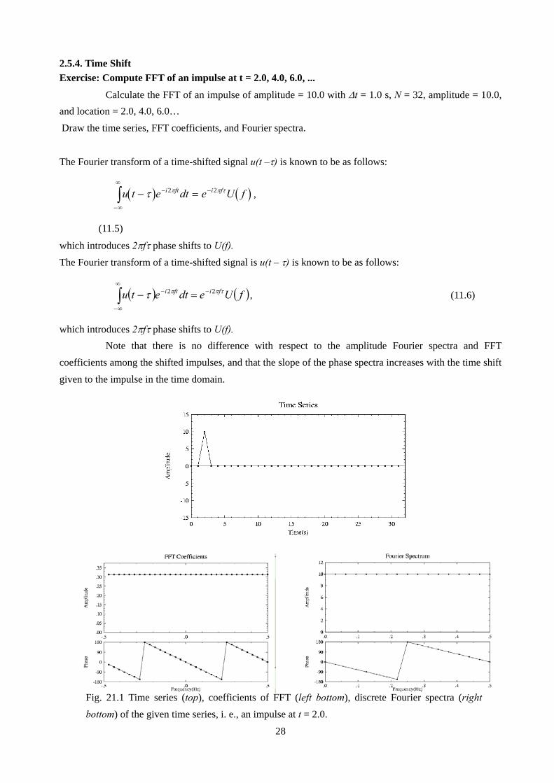
2.5.4. Time Shift Exercise: Compute FFT of an impulse at t = 2.0, 4.0, 6.0, ...
Calculate the FFT of an impulse of amplitude = 10.0 with Δt = 1.0 s, N = 32, amplitude = 10.0, and location = 2.0, 4.0, 6.0… Draw the time series, FFT coefficients, and Fourier spectra.
The Fourier transform of a time-shifted signal u(t –τ) is known to be as follows:
( ) ( )u t e dt e U fi ft i f− =−
−∞
∞−∫ τ π π τ2 2 ,
(11.5)
which introduces 2πfτ phase shifts to U(f). The Fourier transform of a time-shifted signal is u(t – τ) is known to be as follows:
( ) ( )fUedtetu fifti τππτ 22 −∞
∞−
− =−∫ , (11.6)
which introduces 2πfτ phase shifts to U(f). Note that there is no difference with respect to the amplitude Fourier spectra and FFT
coefficients among the shifted impulses, and that the slope of the phase spectra increases with the time shift given to the impulse in the time domain.
Fig. 21.1 Time series (top), coefficients of FFT (left bottom), discrete Fourier spectra (right bottom) of the given time series, i. e., an impulse at t = 2.0.
29
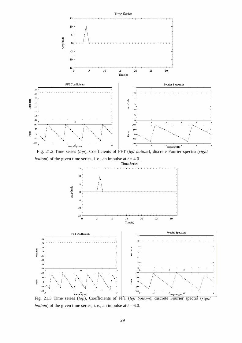
Fig. 21.2 Time series (top), Coefficients of FFT (left bottom), discrete Fourier spectra (right bottom) of the given time series, i. e., an impulse at t = 4.0.
Fig. 21.3 Time series (top), Coefficients of FFT (left bottom), discrete Fourier spectra (right bottom) of the given time series, i. e., an impulse at t = 6.0.

30
2.5.5. Aliasing Exercise: Simulate aliasing effect.
Calculate the cosine wave having a period of 0.8 s (1.25 Hz) with Δt = 1.0 s, N = 32, amplitude = 10.0, damping = 0.0, and phase = 0.0. The frequency of 1.25 Hz is higher than the Nyquist frequency 0.5 Hz. The time series panel below does not appear to be a 1.25-Hz wave. A false peak due to aliasing is observed in the spectrum panels. Aliasing occurs due to the f f f Nyquist= ± ±( )0 2 ambiguity of the frequency. In this example, the peak at
1.25 Hz is folded into 1.25 – 2*0.5 Hz = 0.25 Hz.
Fig. 22 Time series (top), coefficients of FFT (left bottom), discrete Fourier spectra (right bottom) of the given time series, i. e., a cosine function at the frequency higher than the Nyquist frequency.

31
2.5.6. Assumption of Periodicity Exercise:
Calculate a cosine wave period = 7.0 s (0.14 Hz) Δt = 1.0 s, N = 32, amplitude = 10.0, damping = 0.0, phase = 0.0, and consider why a line spectrum at f = 0.14 Hz could not be obtained.
Fig. 23 Time series (top), coefficients of FFT (left bottom), discrete Fourier spectra (right bottom) of the given time series, i. e., a cosine function at the frequency mentioned above.

32
3. Filtering Techniques Recorded signals are often contaminated by AC noise or high-frequency ground noise from
nearby stations. Therefore, various filtering techniques are essential for digital data processing.
3.1. Weighted Moving Average The simplest method to suppress high-frequency components included in a given time series xm
= x(tm) may be moving averages such as
.3
11 +− ++= mmm
mxxx
y
This equation shows a three-point moving average. The output ym is defined by the one-step previous term of the input xm–1, the present term xm, and the future term xm+1. The five-point moving average is given by
.5
2112 ++−− ++++= mmmmm
mxxxxx
y
The performance of the moving average can be estimated by applying it to an impulse of the
unit amplitude located at t = 0.0, because the moving average belongs to linear systems. Fig. 24 shows the Fourier spectra of the output corresponding to the impulse input for the two moving averages mentioned above. As shown here, the moving average can certainly be used to eliminate high-frequency components. However, it is difficult to control the performance and value of parameters such as the cut-off frequency, the slope of the cut-off, etc.
Fig. 24 Fourier spectra of the output from the three-point moving average corresponding to the impulse input (left) and that from the five-point moving average (right). These examples are
calculated with Δt = 1.0 s and N = 64.

33
Fig. 25 Fourier spectra of the output from the weighted moving average corresponding to the impulse input. Left: for the weight coefficients (0.25, 0.5, and 0.25). Right: for the weight
coefficients (–0.25, 0.5, –0.25). These examples are calculated with Δt = 1.0 s and N = 64
The weighted moving average is a similar procedure but with different weight coefficients. This gives a better performance than that given by the simple moving average. For example, the three-point average
,25.05.025.0 11 +− ++= mmmm xxxy
can eliminate high-frequency components, as shown in Fig. 25 (left). Note that this maintains the phase lag at zero for all frequencies. The other example,
,25.05.025.0 11 +− −+−= mmmm xxxy
can eliminate low-frequency components as shown in Fig. 25 (right). Note that the phase lag is maintained at zero for all frequencies. The differentiation of a continuous function x(t),
( ) ( ),txdtdty =
can be approximated by the finite difference,
.111
1mm
mmm x
tx
ttxx
y ⎟⎠⎞
⎜⎝⎛
Δ+⎟
⎠⎞
⎜⎝⎛
Δ−=
Δ−
= −−
This also belongs to the weighted moving average.
These examples show that the weighted moving average can have a good performance. In other words, we can arrange its characteristics by selecting the weight coefficients. By using the idea of the impulse response, we can check the characteristics of its performance. However, we must design the weighted moving average by selecting the weight coefficients in such a way that the characteristics of the performance are obtained as desired.

34
3.2. Convolution—Filtering in the Time Domain In order to understand the methods that are used to design weight coefficients, in this chapter,
the procedure for “convolution” in the time domain is examined.
3.2.1. Convolution Suppose that the Fourier transform of the time dependent functions f(t) and g(t) are F(ω) and
G(ω), respectively. The inverse Fourier transform of the product of F(ω) with G(ω) is given by
( ) ( ) ( ) ( )
( ) ( )
( ) ( )
12
12
12
πω ω ω
πω ω τ τ
τ τπ
ω ω
τ τ τ
ω ω ωτ
ω τ
F G e d F e d g e d
g d F e d
g f t d
i t i t i
i t
−∞
∞
−∞
∞−
−∞
∞
−∞
∞−
−∞
∞
−∞
∞
∫ ∫ ∫
∫ ∫
∫
=⎛
⎝⎜
⎞
⎠⎟
=
= −
( )
.
This integration is referred to as the convolution of two functions f(t) and g(t) in the range ( , )−∞∞. Convolution is usually expressed by an asterisk between two functions.
( ) ( ) ( ) ( ) ( ) ( )f t g t f g t d f t g d* = − = −−∞
∞
−∞
∞
∫ ∫τ τ τ τ τ τ
If f(t) has a non-zero value only in the range t1 < t < t2,
( ) ( ) ( ) ( ) ( ) ( )∫∫−
−
−=−=1
2
2
1
*tt
tt
t
t
dgtfdtgftgtf ττττττ
Mathematically, convolution in the time domain corresponds to the product of the Fourier
transforms in the frequency domain. The time domain operation may have advantages when one of the two time series has a short duration. In such a case, the short time series f(t) is considered as a filter for modifying the input signal g(t). The effect of filtering must be controlled by the spectrum of the filter f(t). Note that the amplitude spectrum of the output is the product of the amplitude spectra of the two original signals and the phase spectrum of the output is the sum of their phase spectra.
3.2.2. Filtering in the Time Domain by Convolution Let us examine the calculation procedures in a computer for the convolution of two time series.
Assume that f(t) has a short duration with non-zero values only within [0, tM].
( ) ( ) ( ) ( ) ( ) .* ∫−
−==t
tt M
dgtftgtfth τττ
In a discretized form,

35
( ) ( ) ( )
( ) ( ) ( ) ( ) ( ) ( ).011 nMnMMnM
n
Mnmmmnn
tgtftgtftgtf
tgtfth
τττ
τ
Δ++Δ+Δ=
Δ=
+−−−
−=−∑
L
This means that the filter time series is reversed and used as the weight coefficients for the weighted moving average, as explained in the previous chapter.
Example: Time domain operation Yilmaz(1994) show a graphical explabnation of the convolution as follows. The convolution of a filter f(t) = (1.0, –0.5) with a signal g(t) = (1.0, 0.0, 0.5). Assume that the sampling interval is equal to 1.0 s. Further, note that M = 1. Reversing the filter f(t): (1, –0.5) changes it into (–0.5, 1).
Output h(t)
Add the product f(tn–m)g(tm ) for m = 0 to M. The sum gives the value h(tn). Shift the moving array one sample to the right and repeat the procedure for adding products. Try to examine whether the same result is given if f(t) and g(t) exchange their roles. (After Yilmaz (1994)).

36
3.3. Feature of Filter Wavelets When a signal is composed of only a few cycles in the time domain, it is called a “wavelet.” A
wavelet is usually considered a transient signal. Undoubtedly, convolution with a wavelet can be considered equivalent to filtering. The characteristics of this filter are directly defined by the frequency spectrum of the filter wavelet. Every weighted moving average belongs to this category. The discussion in the previous chapter gave some typical examples.
Again, it must be noted that the amplitude spectrum of the output is the product of the amplitude spectra of the filter and the input signal, while the phase spectrum of the output is the sum of their phase spectra.
3.3.1. Phase The time series are composed of limited and discrete numbers of sinusoidal functions with a
constant interval of frequency Δf, that is, the reciprocal of the duration T. The wavelet that shows a symmetry around t = 0 and has a positive peak amplitude is the zero phase wavelet. Fig. 26 shows the decomposition of a wavelet into various sinusoids. Note that all the component sinusoids have zero time
shifts. The phase lag is defined by 2πftshift, where tshift is the time shift. If the time shift is zero for all the frequencies, the wavelet is called “zero phase wavelet.” If the time shift is a constant for all frequency components, it is equivalent to a linear phase shift, an example of which is given in Fig. 27. The tangent of
Fig.27 Constant time delay -0.2 sec given to the sinusoidal components same as those in Fig. 26results in a wavelet of the same shape as that in Fig.26 (denoted by an asterisk), except that it is shifted in time by -0.2 sec. Produced newly based on the concept of Yilmaz(1994).
Fig. 26 Decomposition of a band limited symmetric (zero-phase) wavelet (denoted by an asterisk) into a discrete number of sinusoids with no phase lag, but with the same peak amplitude. Produced newly based on the concept of Yilmaz(1994).

37
the line for the phase spectra is proportional to the time shift for the linear phase shift, as shown in Fig. 28. Note that the linear phase shift keeps the waveform constant.
In contrast to the linear phase shift, a
constant phase shift changes the waveform. The wavelet shown in Fig. 29 has the same amplitude spectrum as that in Fig. 26. The difference is their phase spectrum. Note that zero crosses are aligned in Fig. 29, whereas the peaks are aligned in Fig. 26. Fig. 30 shows the way in which the waveform is changed by a constant phase shift. Note that a constant 180-degree phase shift changes the sign of the wavelet. Note the relation of the panels (a) and (c) and panels (b) and (d). The constant phase shift of 180 degree implies a reversal of sign.
The linear and constant phase shifts are
two basic examples of phase change. The combined operation is defined as a + b·frequency, where a is the constant phase shift and b is the tangent of the linear phase shift, gives a time shift with a waveform change. The result is a combination of both effects, as shown in Fig. 31.
Note that the shape of the wavelet can be changed by modifying the phase spectrum even while keeping the amplitude spectrum constant. Several examples for this combination are shown
Fig. 29 Constant 90-degree phase shift given to the sinusoidal components same as those in Fig. 26results in asymmetric wavelet but the zero crossing at t = 0 (indicated by an asterisk). Produced newlybased on the concept of Yilmaz(1994).
Fig.28 Wavelets in the time domain are shifted by th elinear phase shift starting with a zero-phase wavelet (a). The slope of the linear phase function is related to the time shift. Produced newly based on the concept of Yilmaz(1994).

38
in Figs. 32 (a), (b), and (c). An arbitrary change in the phase spectra, however, can break the wavelet. The tangent of the phase shift is called “delay.”
ωφ
dddelay −=
The linear phase shift is an example of constant delay for all frequencies. In general, “delay” can be dependent on the frequency.
Fig. 30 Series of waveform change caused by a constant phase shift starting with the zero-phase wavelet (a). A 90-degree phase shift converts the zero-phase wavelet to an antisymmetric wavelet (b),while a 180-degree phase shift reverses its polarity (c). A 270-degree phase shift reverses the polarity, while making the wavelet antisymmetric (d). Finally, a 360-degree phase shift does not influence the wavelet (e). Produced newly based on the concept of Yilmaz(1994).
Fig. 31 Time-shifted antisymmetric wavelet (denoted by an asterisk) caused by a linear phase shift combined with a constant phase shift for the component sinusoids same as those in Fig.26. Produced newly based on the concept of Yilmaz(1994).

39
Fig. 32 a non-zero-phase spectrum of any form in (b) and (c) modifies the shape of a zero-phase wavelet (a). Produced newly based on the concept of Yilmaz(1994).
Fig. 33 The summation of zero-phase sinusoids with an identical peak amplitude shows that the incresing frequency bandwidth results in the synthesized zero-phase wavelet increasingly compressed. Produced newly based on the concept of Yilmaz(1994).

40
3.3.2. Frequency Components In the previous chapter, wavelets with varying phase spectra and fixed amplitude spectra are
observed. By changing the amplitude spectrum or selecting the frequency contents, the wavelet changes its shape even when its phase spectrum is maintained constant. Here, zero-phase wavelets are used for simplicity. Fig. 33 shows a clear example of the changes in zero-phase wavelets by the selection of frequency contents. As more frequency components are summed, the synthesized zero-phase wavelet is increasingly compressed. If they are summed till the Nyquist frequency, a spike is formed (Fig. 34).
The broader the bandwidth, the more compressed the wavelet; in other words, a shorter wavelet
is obtained. This property also follows from the fundamental concept that the effective time span of a time series is inversely proportional to its effective spectral bandwidth (Fig. 35).
The shape of the frequency spectrum also influences the wavelet shape. Fig. 36 shows a typical case. A short wavelet requires a tapered amplitude spectrum, although the width of the passband for all cases is identical.
Filtering in the frequency domain can be performed by the inverse Fourier transform of the product of the Fourier transforms of the filter and input time series. This is equivalent to the filtering in the time domain that is performed by the weighted moving average of the input time series, the weight coefficients of which are the reversed filter time series. This, in general, can be written as
,221101122 LL ++++++= +−+−−− iiiiii xaxaxaxaxay
where ( LL ,,,,,, 21012 aaaaa −− ) is the filter time
series. If we consider causality, i. e., the idea that the results cannot proceed to the cause, we cannot use the terms of the future xi+1, xi+2,… to obtain the present output yi. Thus,
.01122 iiii xaxaxay +++= −−L
Fig. 34 The output wavelet becomes a spike when the summation includes sinusoids at all frequencies up to the Nyquist frequency. Small dots denote the sampling points at 64Hz. Produced newly based on the concept of Yilmaz(1994).

41
Fig. 35 Incresing bandwidth in the frequency domain (bottom panels) corresponds to more compressed wavelet in the time domain(top panels). Produced newly based on the concept of Yilmaz(1994).
Fig. 36 More gentle slope in the frequency domain(bottom panels) corresponds to smoother wavelet in the time domain (top panels). (a) The steep slopes of the passband cause ripples in the wavelet and the actual amplitude spectrum. (b) A moderate and (c) gentle slope help eliminate the ripples. Produced newly based on the concept of Yilmaz(1994).

42
3.3.3. Causality or Non-Causal Filtering A phenomenon that is the result of another phenomenon (the cause) never occurs before the cause itself does. This is called a “causal relation” or “causality” and it is strictly maintained in the real world. However, in a computer, this relation can be broken. Such a breakage often affects the seismological analyses. The following shows us examples.
Exercise: Filtering in the time domain and in the frequency domain: an example The topics in this chapter can be learned much better by practicing with the distributed software.
Here, the following programs are prepared for practice. FFILT.EXE creates a set of coefficients of Fourier expansion from given bandpass
characteristics. FPRDCT.EXE calculates the product of two given sets of the coefficients of Fourier
expansion, i. e., filtering in the frequency domain. FWVLET.EXE creates a filter wavelet from the given time series that may be obtained by the
inverse Fourier transform of a given set of the coefficients of Fourier expansion.
FCONV.EXE calculates convolution, i. e., filtering in the time domain for a given filter wavelet and input signal.
The programs TESTSIG.EXE, PTIME.EXE, FFT.EXE, PCFFT.EXE, PSPEC.EXE, and IFFT.EXE are also used.
(0) Prepare the test input signal UT1, that is a unit impulse located at t = 8.0 s of the time series with N =
64, Δt = 1.0, and its Fourier transform UF1 by using TESTSIG.EXE and FFT.EXE (Fig. 36a).
Fig. 36a Test input signal for the exercise UT1 and its spectra. Time dependence (upper panel), the coefficients of Fourier expansion (lower left panel), and Fourier spectra (lower right panel).
The impulse is located at t = 8.0 s of the time series with N = 64, Δt = 1.0. The linear phase shift due to the shifted location of the impulse is shown.
43
Filtering in the frequency domain: (1) Design a band pass filter in the frequency domain by using FFILT. The number of data for the
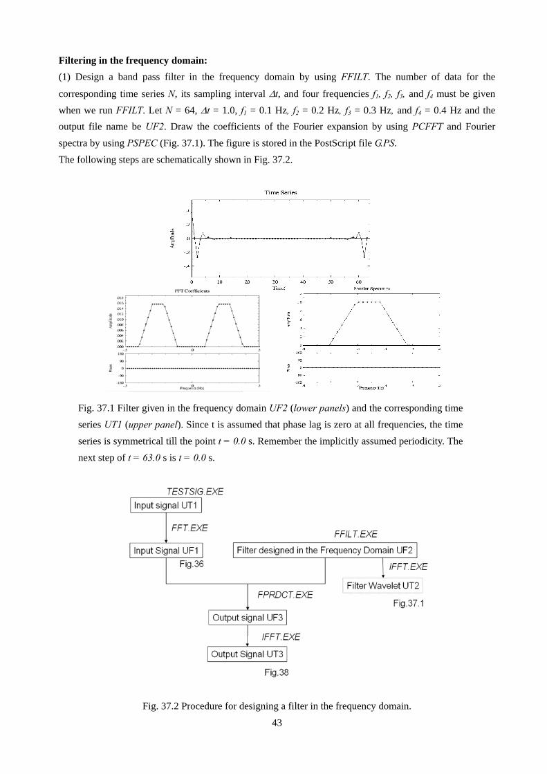
corresponding time series N, its sampling interval Δt, and four frequencies f1, f2, f3, and f4 must be given when we run FFILT. Let N = 64, Δt = 1.0, f1 = 0.1 Hz, f2 = 0.2 Hz, f3 = 0.3 Hz, and f4 = 0.4 Hz and the output file name be UF2. Draw the coefficients of the Fourier expansion by using PCFFT and Fourier spectra by using PSPEC (Fig. 37.1). The figure is stored in the PostScript file G.PS. The following steps are schematically shown in Fig. 37.2.
Fig. 37.1 Filter given in the frequency domain UF2 (lower panels) and the corresponding time series UT1 (upper panel). Since t is assumed that phase lag is zero at all frequencies, the time series is symmetrical till the point t = 0.0 s. Remember the implicitly assumed periodicity. The next step of t = 63.0 s is t = 0.0 s.
Fig. 37.2 Procedure for designing a filter in the frequency domain.
44
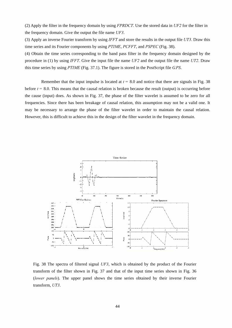
(2) Apply the filter in the frequency domain by using FPRDCT. Use the stored data in UF2 for the filter in the frequency domain. Give the output the file name UF3. (3) Apply an inverse Fourier transform by using IFFT and store the results in the output file UT3. Draw this time series and its Fourier components by using PTIME, PCFFT, and PSPEC (Fig. 38). (4) Obtain the time series corresponding to the band pass filter in the frequency domain designed by the procedure in (1) by using IFFT. Give the input file the name UF2 and the output file the name UT2. Draw this time series by using PTIME (Fig. 37.1). The figure is stored in the PostScript file G.PS. Remember that the input impulse is located at t = 8.0 and notice that there are signals in Fig. 38 before t = 8.0. This means that the causal relation is broken because the result (output) is occurring before the cause (input) does. As shown in Fig. 37, the phase of the filter wavelet is assumed to be zero for all frequencies. Since there has been breakage of causal relation, this assumption may not be a valid one. It may be necessary to arrange the phase of the filter wavelet in order to maintain the causal relation. However, this is difficult to achieve this in the design of the filter wavelet in the frequency domain.
Fig. 38 The spectra of filtered signal UF3, which is obtained by the product of the Fourier transform of the filter shown in Fig. 37 and that of the input time series shown in Fig. 36 (lower panels). The upper panel shows the time series obtained by their inverse Fourier transform, UT3.

45
Filtering in the time domain: (5) Extract the filter wavelet from the time series stored in the file UT2 by using FWVLET. Give the output the file name FWV1. We have to select either a causal filter or a zero-phase filter. Here, we select a zero-phase filter with 13 coefficients.
Fig. 39.1 Procedure for designing a filter in the time domain
Fig. 39.2 Output time series from the filtering in the time domain with the truncated filter wavelet designed for zero phase filtering, UT4 (upper panel), and its spectra, UF4 (lower panels). Note the stability of the output time series and the negligible phase change in the pass band in comparison with Fig. 38. The change in the amplitude spectral shape is the effect of the truncation of the wavelet.

46
(6) Apply the filter in the time domain obtained in (5) by using FCONV. The input filter file name is FWV, the file name of the input time series is UT1, and the output file name is UT4. Draw the time series stored in UT4 by using PTIME and compare it with the figures for UT3 obtained in (3). Due to the truncation of the filter time series, the time series stored in UT4 is slightly different from that in UT3. Check the performance of the filtering by using FFT, PCFFT, and PSPEC with UT4 (Fig. 39.2). (7) Extract the filter wavelet from the time series stored in the file UT2 by using FWVLET. Give the output file the name FWV2. We must select either a causal filter or a zero-phase filter. In this case, we select a causal filter with 6 coefficients. (8) Apply the filter in the time domain obtained in (5) by using FCONV. The input filter file name is FWV, the file name of the input time series is UT1, and the output file name is UT5. Draw the time series stored in UT4 by using PTIME and compare it with the figure for UT3 obtained in (3). The output in this case is clearly different from the results obtained in the time domain in (6) and from those in (3). Note that the causality is satisfied in the time domain. Check the performance of the filtering by using FFT, PCFFT, and PSPEC with UT5 (Fig.40). (9) Repeat the procedures explained above after changing the number of weight coefficients for FWV and compare them. This example shows the problems with designing a filter wavelet with desirable characteristics both in the time frequency domains. In general, however, the filtering in the frequency domain works well for zero-phase filtering. .
Fig. 40 Output time series from the filtering in the time domain with the truncated filter wavelet designed for zero phase filtering UT5 (upper panel) and its spectra UF5 (lower panels). Note that the causality with Fig.36 is maintained. The change in the amplitude and phase spectral shape is the effect of the truncation of wavelet. The truncation of a former half of the filtering wavelet results in the phase shift by filtering and reduction in the amplitude spectra even in the pass band.

47
3.4. Recursive Filter In the previous chapter, we have checked the features of the filter wavelet that can be replaced
by using the weighted moving average. The general formula of this filter is given by the following equation after taking causality into account.
.2211001122 LL −−−− ++=+++= iiiiiii xaxaxaxaxaxay
We have checked that the differentiation can be expressed by the weighted moving average that belongs to this category, i. e.,
.111
1mm
mmm x
tx
ttxx
y ⎟⎠⎞
⎜⎝⎛
Δ+⎟
⎠⎞
⎜⎝⎛
Δ−=
Δ−
= −−
Let us consider the integration given by
( ) ( ) .0∫=t
dxty ττ
The discretization gives
.0
∑=
⋅Δ=m
nnm xty
This implies the relation,
.1 mmm xtyy ⋅Δ+= −
Note that the term in the output that corresponds to the single step after ym–1 is used to construct the output for the current ym. The filter that has had such a recursive usage of the output in the past is called a “recursive filter” (Fig. 40). The general formula for the recursive filter after taking the causality into account is given by
).( 2211221100 LL ++−++= −−−− iiiiii ybybxaxaxayb
Fig. 41 Block diagram for the filter that can be expressed by the weighted moving average (upper) and the recursive filter (lower).

48
Fig.42 Complex s-plain
3.4.1. Laplace Transform The Fourier transform of a continuous function has been defined previously. The meaning of
Fourier transform is basically an expansion of the function on the basis of the sinusoidal function exp(iωt). The sinusoidal function with an exponential decay or amplitude exp((σ+ iω)t) can also be used as the basis for expansion. Such an integral transform is called Laplace Transform.
The Laplace transform and its inverse transform are defined by the following (here s = σ + iω).
( ) ( )
( ) ( ) .21
,0
∫
∫+
−
∞−
=
=
ωγ
ωγπ
i
i
st
st
dsesFi
tf
dtetfsF
The Laplace transform F(s) is defined in the complex s-domain (Fig. 42).
3.4.2. Filter Operation in the s-domain The instrument characteristics of seismometers, seismographs, and every electronic circuit can
be described by an appropriate transfer function. The analog transfer function may be given by using the variable for the Laplace transform as follows:
( )T s A s A s A s A s AB s B s B s B s B
s iLL
LL
MM
MM
=+ + + + ++ + + + +
= +−−
−−
11
22
1 0
11
22
1 0
L
L, .σ ω (12)
The stability of this analog filter is obtained simply when all the solutions of the equation,
B s B s B s B s BMM
MM+ + + + + =−
−1
12
21 0 0L ,
sn has to satisfy the following condition for the stability of the system. ( )Re sn = <σ 0 .
Otherwise, the circuit becomes a noise generator.
σ
iω
0

49
Example: Simple Moving Coil Type Seismometer (Transfer function in the s-domain) The equation of motion for a pendulum's displacement in a seismometer relative to the ground
x(t) induced by the ground motion y(t) is given by
,2 2
22
002
2
dtydx
dtdxh
dtxd
−=++ ωω (13)
where ω0 denotes the natural frequency of the pendulum and h denotes the damping factor. Applying the Fourier transform to both sides yields
− + + =ω ω ω ω ω20 0
2 22x ih x x ym m m m .
Thus, the response in the frequency domain is given by
( ) ( )− =
− −x y
ihm m
11 2 0 0
2ω ω ω ω.
This response belongs to a high pass filter, and therefore, the seismometer has an equivalent digital filter. Define the transfer function in the frequency domain,
( )( ) ( )
( )( ) ( )
.221
1200
2
2
200 ωωωω
ωωωωω
ω++
=−−
=−=ihi
iih
yxiT mm (14)
The Laplace transform of Eq. (14) gives the transfer function in the s-domain. The substitution of iω with s in Eq. (15) gives the result:
( ) ( )( ) .
2 200
2
2
ωω ++=−=
shss
sYsXsT (15)
The solutions obtained when the denominator = 0 are called “poles.” In contrast, the solutions of the numerator = 0 are called “zeros,” because these cause the transfer function to be equal to zero. Eq. (12) can be factorized by using these poles and zeros as follows.
( ) ( ) ( )( )( ) ( )( )
( ) ( )( )( ) ( )( )
T s AB
s s s s s s
s s s s s sG
s s s s s s
s s s s s sL
M
L
M
L
M
= ⋅− − −
− − −= ⋅
− − −
− − −
020
10
2 10
020
10
2 1
L
L
L
L. (16)
The suffix 0 denotes the “zero” point. As shown, “zeros” and “poles” determine the transfer function with a constant G0. If s coincides with one of the poles, T(s) becomes infinite. If s coincides with one of the zeros,
T(s) becomes zero. Actually, s = σ + iω moves only along the imaginary axis in the complex s-plane, and poles must locate at σ < 0 in stable systems. Then, s cannot coincide exactly with any of the poles. Poles located near the imaginary axis can induce resonance. If one of the zeros lies on the imaginary axis, T(s) becomes zero sharply at the corresponding frequency. This feature is important for the design of a notch filter. The pole-zero representation of an analog transfer function provides a method for the design of circuits. Readers are recommended to study books on electronics, especially on active filters for more information. Several examples for simple transfer functions will be given in the following description.

50
Today, many seismic observation organizations release their data to the public via the Internet so that any researcher can use them. Some of these organizations provide information on instrumental characteristics using the pole-zero representation. Hence, it may be useful to show the method of reconstructing the transfer function in the frequency domain from a given value of poles and zeros.
At an angular frequency ω, the variable of the Laplace transform s is located at (0, iω).
)( mss − in the denominator of Eq. (13) implies the distance between s = (0, iω) and the pole sm taking
phase into consideration as well. Namely,
))exp(arg()()( mmm ssssss −−=− .
When all poles and zeros are similarly considered, the following relations are obtained:
( ) ( ) ( )( )( ) ( )( )
( ) ( ) ( ) ( ){ }.argargargargexp 101
0
12
01
02
0
0
12
01
02
0
0
ssississississssssssssss
G
ssssssssssssGsT
MLM
L
M
L
−−−−−−++−⋅−−−
−−−=
−−−−−−
⋅=
LLL
L
L
L
Suppose that XL…X2, X1 denote the absolute values of )( mss − and ΘL…Θ2, Θ1 denote the absolute
values of their phases. Similarly, xM…x2, x1 and θM…θ2, θ1 for poles. Then,
( ) { }.exp 1112
120 θθ iiii
xxxXXXGsT ML
M
L −−−Θ++Θ⋅= LLL
L
This shows that the transfer function can be reconstructed from the given values of poles and zeros by a direct graphical measurement on the complex s-plane without any special software. This simple feature is one of the advantages of introducing Laplace transforms in the analysis of transfer functions.
Example: Simple Moving Coil Type Seismometer (Poles and Zeros) Eq. (15) is factorized in the following manner.
( ) ( )( )
( )( )( )( ) .
2 12
01
02
200
2
2
ssssssss
shss
sYsXsT
−−−−
=++
=−=ωω
The solutions of the equation, achieved by equating the denominator to zero are ( )120 −±−= hhs ω .
This gives the pole position at
( )200 1, hh −− ωω , ( )2
00 1, hh −−− ωω for h < 1.0, under-damped case,
( ).0,0ω− doubled for h = 1.0, critically damped case,
( )( ).0,120 −−− hhω , ( )( ).0,12
0 −+− hhω for h > 1.0, over-damped case.
For all these three cases, the poles are located in the left half of the s-plane. This guarantees the stability of the system. The doubled zeros are located at (0,0).
51
3.4.3. Z-transform Remember the discrete Fourier transform:
.2
,1
,
1
1
tNkwhere
eXtN
x
extTCX
k
N
k
timkm
N
m
timmkk
k
k
Δ=
Δ=
Δ==
∑
∑
=
Δ
=
Δ−
πω
ω
ω
(17)
Xk has a certain physical meaning. Let us change Eq. (17) slightly in the following way.
.~1
,~
1
1
∑
∑
=
Δ
=
Δ−
=
=
N
k
timkm
N
m
timmk
k
k
eXN
x
exX
ω
ω
This gives an abstract quantity in the transformed domain. A new variable is introduced as
.ti kez Δ= ω (18) Thus,
.~1
,~)(
1
1
∑
∑
=
=
−
=
==
N
k
kkm
N
m
mmkm
zXN
x
zxXxZ
(19)
This new integral transform for discrete systems is called z-transform. Eq. (18) can be extended to relate
the discrete z-transform with a continuous Laplace transform with s = σ + iω.
.tsez Δ= (20) The product with z implies a time shift of Δt toward the future, whereas that with z–1 implies one toward the
Re z
Im z
0 1
1
-1
-1
Fig. 43 Complex z-plain. The left half of the complex s-plane is mapped into a unit circle
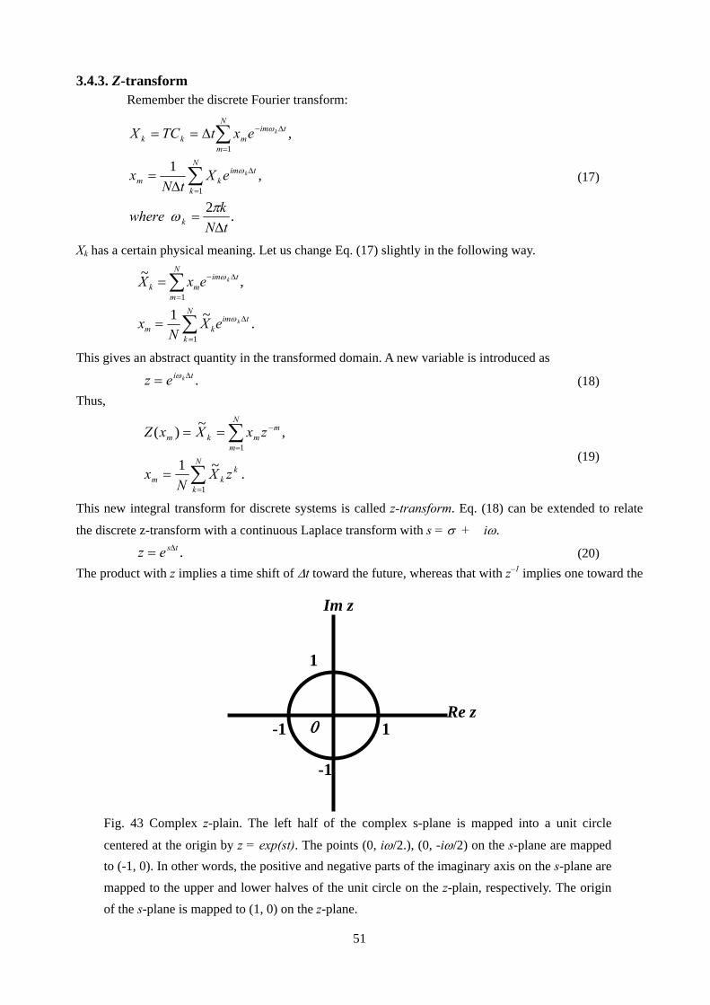
centered at the origin by z = exp(st). The points (0, iω/2.), (0, -iω/2) on the s-plane are mapped to (-1, 0). In other words, the positive and negative parts of the imaginary axis on the s-plane are mapped to the upper and lower halves of the unit circle on the z-plain, respectively. The origin of the s-plane is mapped to (1, 0) on the z-plane.

52
past.
3.4.4. Filter Operator in the Z-domain Suppose x(t) denotes the input time series; X(ω), its Fourier spectrum; y(t), the filtered output;
Y(ω), its spectrum; and F(ω), the spectrum of the applied filter. Then,
( ) ( ) ( ).ωωω XFY = (21) Suppose the filter spectra can be written, e. g., in the following form in order to facilitate ease of discussion.
( )( ) ,22
110
22
110
−−
−−
++++
=zbzbbzazaazF ω (22)
Eq. (21) gives the relation
[ ] ( ) [ ] ( ).22
110
22
110 ωω XzazaaYzbzbb −−−− ++=++
The inverse Fourier transform of both sides gives
( ) ( ) ( ) ( ) ( ) ( ),22 210210 ttxattxatxattybttybtyb Δ−+Δ−+=Δ−+Δ−+
because of the relation
( ) ( ) ( ) .21
21 )( tntydeYdeYz tntitin Δ−== ∫∫
∞
∞−
Δ−∞
∞−
− ωωπ
ωωπ
ωω
Then, the filtered output can be calculated rapidly with a defined value of coefficients, a few preceding data of the input time series, and a few preceding data of the output. For Eq. (22),
( )
( )
y ab
x
yb
a x a x b y
yb
a x a x a x b y b y jj j j j j j
00
00
10
0 1 1 0 1 0
00 1 1 2 2 1 1 2 2
1
1 2
=
= + −
= + + − − ≥
⎫
⎬
⎪⎪⎪
⎭
⎪⎪⎪− − − − ,
. (23)
This shows an example for a recursive filter operating in the time domain. The filter F(ω) might give a phase lag. In order to compensate for the phase lag, namely, in order to apply a zero-phase filter, inverse the time axis and apply the same filter in such way that
( )
( )
y ab
x
yb
a x a x b y
yb
a x a x a x b y b y j
N N
N N N N
N j N j N j N j N j N j
=
= + −
= + + − − ≥
⎫
⎬
⎪⎪⎪
⎭
⎪⎪⎪
−
− − − −
− − − + − + − + − +
0
01
20
0 2 1 1 1 1
00 1 1 2 2 1 1 2 2
1
1 3,
. (24)
Of course, we can employ more coefficients al and bm if necessary. The general form of Eq. (22) may be

53
( ) .,0
11
22
)1(1
01
12
2)1(
1 tiM
MM
M
LL
LL ez
bzbzbzbzbazazazaza
zF Δ−−−−
−−
−−−−−
−
=+++++
+++++= ω
L
L (25)
The corresponding recursive filter may be
{
}.)(
1
112211
11221100
MjMMjMjj
LjLLjLjjjj
ybybybyb
xaxaxaxaxab
y
−+−−−−
−+−−−−
++++−
+++++=
L
L (26)
This filter given by Eq. (25) is sometimes called a transfer function by analogy with the filters of electronic circuits, which are analog filters. Since the denominator of Eq. (25) controls the feedback part of Eqs. (23) and (24), bm must be selected carefully in order to avoid any instability in the filtering. The transform z =
exp(sΔt) maps the left half of the complex s-plane to the unit circle centered at the origin on the complex z-plane. Therefore, a stable and causal filtering requires that all the solutions of the equation
( 1) 2 1
1 2 1 0 0M MM Mb z b z b z b z b− − − − −
−+ + + + + =L
zn must satisfy the condition
.1<nz (27)
Additionally, if there are no zeros outside the unit circle on the complex z-plane, it is called minimum phase condition.
Focus on the direct coincidence of the coefficients of a filter wavelet in the time domains shown in Eq. (23) and Eq. (24) with the coefficients used in the transfer function in the Z-domain that is shown in Eq. (22). This shows that the analysis of the transfer function in the Z-domain gives the value of the coefficients for recursive filtering in the time domain.
The transfer function given in the frequency domain and that given in the s-domain are analogous functions, whereas that represented by a recursive filter is applied to a discrete time series in the computer. Z-transform behaves like an interpreter at the border between two worlds that are different each other—one a continuous world and the other a digital one.
The relation between the transfer function in the Z-domain and that in the s-domain is given
approximately by the so called bilinear transform:
.
21
21
,112
1
1
st
st
zzz
ts
⋅Δ−
⋅Δ+
=+−
⋅Δ
= −
−
(28)

54
This is an approximation of Eq. (18) that is equivalent to the following:
( ).ln1 zt
sΔ
=
The discrete angular frequency ωk is also transformed. For z = exp(iωkΔt), the bilinear transform gives
( ).2tan2112 t
ti
ee
ts kti
ti
k
k
Δ⋅Δ
=+−
⋅Δ
= Δ−
Δ−
ωω
ω
Since s = iω for σ = 0,
( ) ( )2tan22tan2 1 tt
ortt kk Δ⋅
Δ=Δ⋅
Δ= − ωωωω (29)
This shows the distortion of the continuous angular frequency ω by the bilinear transform to the discrete one ωk (Fig. 44.1). To compensate this distortion, a warped angular frequency
( )2' tan 2c c tt
ω ω= ⋅ ΔΔ
(30)
is introduced (Sherbaum(1996)). The critical angular frequencies cω of the continuous transfer function
are first converted to the corresponding warped angular frequencies c'ω , and then the bilinear transform
using the warped ones is applied to obtain the equivalent discrete transfer function (Fig. 44.2). Eq. (30)
shows that c'ω tends to cω for a small value of
Nyquist
c
Sampling
cc
ff
fft
⋅==Δ
ππω
22
This means that considering the warped frequency is not necessary for frequencies that are considerably smaller than the Nyquist frequency. The natural frequency of a seismometer is usually much smaller than the Nyquist frequency, whereas the anti-aliasing filter has a cut-off frequency that is comparable with the Nyquist one.
Fig. 44.1 Mapping of the continuous angular frequency ω on to the discrete frequency ωk. This is an example of Δt=0.01, N=1024. The Nyquist angular frequency is π/Δt.

55
Fig. 44.2 Schematic drawing that shows how warped frequency works.
Comparison of Bilinear Transform with Z-Transformat 100Hz sampling
-1.5
-1.0
-0.5
0.0
0.5
1.0
1.5
2.0
2.5
3.0
3.5
0.0 10.0 20.0 30.0 40.0 50.0
Frequency
Re(z):z-transform Im(z):z-transform
Re(z):Bilinear Transform Im(z):Bilinear Transform
Fig. 44a Example of a comparison of bi-linear transform with z-transform for Δt = 0.01 s. The difference is negligible at frequencies less than 10 Hz.

56
Example: Simple Moving Coil Type Seismometer (z-transform and equivalent recursive filter) Eq. (15) is factorized in the following manner:
( ) ( )( )
( )( )( )( ) .
2 12
01
02
200
2
2
ssssssss
shss
sYsXsT
−−−−
=++
=−=ωω
This reduces to the following with frequency warping as given by Eq. (30).
( ) .''2 200
2
2
ωω ++=
shsssT (31)
Applying the bilinear transformation to Eq. (31) gives a simulated transfer function in the z-domain,
( )
( )( ) ( )( ) ( )
,
12
tan112
tan21
1
2tan
11
2tan2
11
11
22
110
22
110
210211021
21
021
10
2
1
1
2
1
1
−−
−−
−−−−
−
−
−
−
−
−
−
++++
=
+⎟⎠⎞
⎜⎝⎛ Δ
++−⎟⎠⎞
⎜⎝⎛ Δ
+−
−=
⎟⎠⎞
⎜⎝⎛ Δ
+⎟⎟⎠
⎞⎜⎜⎝
⎛+−
⎟⎠⎞
⎜⎝⎛ Δ
+⎟⎟⎠
⎞⎜⎜⎝
⎛+−
⎟⎟⎠
⎞⎜⎜⎝
⎛+−
=
zbzbbzazaa
zt
zzt
hz
z
tzzt
hzz
zz
zT
ωω
ωω
(32)
where
( ) ( )( )
( ) ( ).2tan2tan21
,2tan22
,2tan2tan21
,0.1,0.2,0.1
02
02
02
1
02
00
210
tthb
tb
tthb
aaa
Δ+Δ−=
Δ+−=
Δ+Δ+=
=−==
ωω
ω
ωω
These coefficients of the recursive filter give an approximately equivalent discrete transfer function.

57
Exercise: Filter Equivalent to a Simple Moving Coil Type Seismometer—1. The program DSEISM.EXE calculates the coefficients of the recursive filter equivalent to the
relative motion of the pendulum mass of a seismometer and applies the recursive filter to an input time series. (1) Prepare an input time series by using TESTSIG.EXE. An impulse of a unit amplitude at t = 0.0 s will
give you the response characteristics of the filter. For example, use Δt = 0.05 s and N = 128. (2) Run DSEISM.EXE with a natural period T0 = 0.5 s, damping factor h = 0.71, Δt = 0.05, and gain G0
=1.0. (3) Draw the filtered time series by using PTIME.EXE and its Fourier spectra by using FFT.EXE and
PSPEC.EXE. An example is shown in Fig. 45.1. (4) Repeat the above procedure with different values of the natural period and damping factor.
Fig. 45.1 Filtered time series and its Fourier spectra obtained by DSEISM.EXE. These are equivalent to the impulse response of the relative motion of a pendulum mass of a
seismometer with the natural period T0 = 0.5 s, the damping factor h = 0.71, Δt = 0.05, and gain G0 = 1.0. The phase at zero frequency should converge to 180 degrees. However, to avoid division by zero, it is forced to be zero.

58
Example: Filter equivalent to a Simple Moving Coil Type Seismometer— 2 In the previous example, the recursive filter that gives the relative displacement of a pendulum
–xm for ground displacement ym is given. Usually, the data obtained by a digital recorder are given numerically and a constant is given for conversion into volts. The potential difference, which is the output from seismometer, is given as follows:
( ) ,0
0m
s
sm xi
RRRGe ω
+=
where (iω) shows the effect of differentiation due to a moving coil type transducer; R0, the coil resistance; Rs, the shunt resistance; and G0, the product of the sensitivity of the seismometer with the conversion constant of a digital recorder. Therefore, the system response is
( )( ) ( )
.21 2
000
0
ωωωωω
−−⋅
+=
ihi
RRRG
ye
s
s
m
m
Fig. 45.2 shows its frequency dependency.
Fig. 45.2 Response of the recursive filters calculated by the formula written above in this page. Dashed line: Filter equivalent to the relative motion of pendulum mass of a simple moving coil type seismometer, against ground displacement. Solid line: Filter equivalent to the voltage change between two output terminals of a simple moving coil type seismometer, against ground displacement. The parameters used are T0=0.5, h=0.71.
Moving Coil Type Seismometer
0.01
0.1
1
10
100
1000
0.1 1 10 100
Frequency
Am
plitude
Relative Motion of Pendulum Mass Output Voltage

59
This has an equivalent digital filter. The corresponding transfer function in the s-domain is
( ) .,2 0
0200
2
3
s
s
RRRGG
shssGsT
+=
++⋅=
ωω (33.1)
The solutions of the equation, i. e., the denominator is equal to zero, are
( )120 −±−= hhs ω .
This gives the pole position at
( )200 1, hh −− ωω , ( )2
00 1, hh −−− ωω for h < 1.0, under-damped case,
( )0 , 0ω− doubled for h = 1.0, critically damped case,
( )( )20 1 ,0h hω− − − , ( )( )2
0 1 ,0h hω− + − for h > 1.0, over-damped case.
However, the numerator gives a tripled zero at (0, 0). By using the warping frequency, the transfer function is given approximately as follows:
( ) ,33
22
110
33
22
110
−−−
−−−
++++++
=zbzbzbbzazazaa
zT (33.2)
where
,.,3,3, 3210 GaGaGaGa −==−==
( ) ( ) ( ){ }( ) ( ) ( ){ }( ) ( ) ( ){ }( ) ( ) ( ){ }.2tan2tan212
,2tan32tan212
,2tan32tan212
,2tan2tan212
02
03
02
02
02
01
02
00
tthtb
tthtb
tthtb
tthtb
Δ+Δ−⋅Δ=
Δ+Δ−−⋅Δ=
Δ+Δ+−⋅Δ=
Δ+Δ+⋅Δ=
ωω
ωω
ωω
ωω

60
Example: Reconstruction of Transfer Function from Given Poles and Zeros Suppose that the following data are given for an observation system. In fact, these data are for a STS—2 feedback type seismometer. Normalization factor: A0 = 5.42787E+07 Normalization frequency: 0.02 (Hz) Complex zeros: i real part imaginary part Index 0 0.000000E+00 0.000000E+00 X0 1 0.000000E+00 0.000000E+00 X1 Complex poles: i real part imaginary part Index 0 –1.247510E+02 –4.171480E+02 x0 1 –1.247510E+02 4.171480E+02 x1 2 –4.873870E–02 –1.552120E–02 x2 3 –4.873870E–02 1.552120E–02 x3 4 –2.513300E+02 0.000000E+00 x4 Sensitivity: G0 = 6.291456E+08 (digit/(M/s)) Frequency of sensitivity: 0.02 (Hz) The normalized amplitude spectra of the transfer function are given as follows:
( )( )( ) ( )( )∏∏
==
−+−=
−
−⋅−= 4
0
22
2
4
0
10
ImRe0
~
mmm
mm xxxs
XsXsT
ω
ωω
The normalizing factor A0 is the reciprocal of this value at f = 0.02 (Hz). ( ) 0.1~0 =ωTA at f = 0.02 Hz.
The reconstructed transfer function is given as follows:
( )( )( ) ( )( )∏
=
−+== 4
0
22
200
00
ImRe
~)(
mmm xx
AGsTAGTω
ωω
For phase spectra,
( )( )∑∑
=
−
= ⎭⎬⎫
⎩⎨⎧
⎟⎟⎠
⎞⎜⎜⎝
⎛−−
−=4
0
11
0 Re0Im
tan2
))((m m
m
l xx
TArgωπω
The first term corresponds to two zeros at the origin. These spectra can be calculated even with a handy calculator.
Re s
Im s
X0, X1
x1
x0
x3
x2
x4
Fig. 45.3 Configuration of poles and zeros, for the example.

61
Fig. 45.4 Amplitude (top) and phase (bottom) response of an STS-2 feed back type seismometer. These are calculated by the formula using poles and zeros data given in the previous page. The calculations were performed easily in Microsoft Excel.
Phase Response
-300
-250
-200
-150
-100
-50
0
50
100
0.01 0.1 1 10 100 1000
Frequency(Hz)
Phas
e(D
egr
ee)
Amplitude Response
1.00E+05
1.00E+06
1.00E+07
1.00E+08
1.00E+09
1.00E+10
0.01 0.1 1 10 100 1000
Frequency(Hz)
Am
plitude
(C
ounts
/(M
/S
ec))

62
3.4.5. Analog Filters and their Transfer Functions Several electronic analog filters are commonly used in seismometry. Their transfer functions are
introduced here. Naturally, each circuit has its equivalent digital filter.
(1) RC filter: One of the simplest electronic circuits is an RC filter that is composed of a resistor and a capacitor, as shown in Fig. 46.
High Pass RC Filter
If the resistor is connected parallel to the output (Fig. 46 top), it is a high pass filter. Suppose x(t) and y(t) denotes the input and output voltage imbalance, respectively. The equation for a high pass filter is as follows:
),()(
),()(
),()()(
tytRI
tVdtdCtI
txtVty
c
c
=
=
=+
(34.1)
where R and C denotes the resistance and the capacitance integrated in the circuit (Fig. 46 top left); I(t), the current that passes through R and C; and Vc, the voltage across the capacitor. This formula gives
).()(1)( txdtdty
CRty
dtd
=+ (34.2)
Fig. 46 (Top) RC high pass filter. Its circuit, transfer function, and response characteristics. (Bottom) RC low pass filter.

63
The transfer function is given by the Laplace transform of Eq. (34.2).
( ) .1, 00
RCwheres
ssT =+
= ωω (34.3)
The amplitude spectra are drawn schematically in Fig. 46 top right.
Low Pass RC Filter If the capacitor is connected parallel to the output, it works as a low pass filter (Fig. 46 bottom).
The low pass filter shown in Fig. 46 bottom left corresponds to the following equation.
),()(
),()()(
tydtdCtI
txtytRI
=
=+
(35.1)
This can be combined into
).()()( txtytydtdRC =+ (35.2)
The transfer function is given by the Laplace transform of (35.2).
Fig. 47 Schematic circuit of an active filter composed of OpAmps. Reproduced based on Yanagisawa and Kanematsu (1980)

64
( ) .1, 00
RCwheres
sT c =+
= ωω
ω (35.3)
The amplitude spectra are drawn schematically in Fig. 46 bottom right.
(2) Active filter. Today, many electronic circuits with known characteristics are widely used for filtering. Some
of those characteristics have their proper names. The requirements for the filters may be flat amplitude characteristics in the pass band, sharp cutoff, and flat delay characteristics in the pass band. The last implies linear phase characteristics because delay is defined as phase differentiated by the angular frequency.
A Butterworth filter has its amplitude characteristics as
( )( )
,1
12n
c
sTωω+
=
where ωc is the cutoff angular frequency. n denotes the order of the filter and the slope of amplitude characteristics in the stop frequency band. In other words, an n-order filter has a decay of 20 n db/oct. The transfer function itself is given for a low pass filter
( )( ) ( )( )
( ) ( ) ( ) ( )( ),,
,,
200
2
20
200
2
20
noddforsQss
sT
nevenforsQs
sT
ccac
a
cc
Ω+Ω+
ΩΠ
Ω+Ω
=
Ω+Ω+
ΩΠ=
ωωω
ωω
and for a high pass filter
( )( ) ( )( )
( ) ( ) ( ) ( )( ),,
,,
200
2
20
200
2
20
noddforsQss
sT
nevenforsQs
sT
ccac
a
cc
Ω+Ω+
ΩΠ
Ω+Ω
=
Ω+Ω+
ΩΠ=
ωωω
ωω
where ωc is the cut-off angular frequency; other coefficients are given in the following table.
Table 10 Coefficients for Butterworth filter
n Q Ω0 Ωa C1 C2 C3
2 0.707107 1.000000 --- 1.4142 0.7071 --- 3 1.000000 1.000000 1.000000 1.3926 3.5468 0.2025 4 0.541196 1.000000 --- 1.0824 0.9239 ---
1.306536 1.000000 --- 2.6131 0.3827 --- 5 0.618034 1.000000 1.000000 1.3541 1.7529 0.4213
1.618034 1.000000 --- 3.2361 0.3090 ---

65
The value of Cn (n = 1, 2, 3) in Table 10 corresponds to the actual value of capacitor Ca (a = 1, 2, 3) in Fig.
47 (right) but normalized one, i.e., Ca = Cn/ωcR, where R is the resistance selected in advance. For high pass filter (Fig. 47 left), Rn (n = 1, 2, 3) are calculated by 1/Cn (n = 1, 2, 3) in Table 10. The value of the
actual resistor Ra (a = 1, 2, 3) in Fig. 47 (left) is given by Ra = Rn/ωcC, where C is the value of the capacitance selected in advance.
Butterworth filter has plane amplitude characteristics in the pass frequency band and is used for shaping of the spectra. The delay characteristics of this filter, however, are not flat even in the pass band. These have a peak of delay around the cut off frequency. This means that the shape of the signal around the cut off frequency in the time domain is considerably distorted by filtering operation.
Chevyshev filter : If we allow the ripple in the pass band, we can perform a sharp cut off. Chevyshev filter belongs to this category. The transfer function is given for low pass filter
( )( ) ( )( )
( ) ( ) ( ) ( )( ),,
,,10
1
200
2
20
200
2
20
10/
noddforsQss
sT
nevenforsQs
sT
ccac
a
ccRp
Ω+Ω+
ΩΠ
Ω+Ω
=
Ω+Ω+
ΩΠ=
ωωω
ωω
and for a high pass filter
( )( ) ( )( )
( ) ( ) ( ) ( )( ),,
,,10
1
200
2
20
200
2
20
10/
noddforsQss
sT
nevenforsQs
sT
ccac
a
ccRp
Ω+Ω+
ΩΠ
Ω+Ω
=
Ω+Ω+
ΩΠ=
ωωω
ωω
where Rp is the ripple amplitude in a pass band measured in (db).
Fig. 48 Amplitude and delay of (a) Butterworth filter and (b) Chevyshev filter in the frequency domain. Both are plotted for the case of a low pass filter

66
The coefficients are given in the following table.
Table 11 Coefficients for Chevyshev filter with ripple of 0.25 db in the pass band
n Q Ω0 Ωa C1 C2 C3
2 0.809254 1.453972 --- 1.1132 0.4249 --- 3 1.508026 1.156992 0.767223 1.6110 6.8272 0.0885 4 0.657249 0.674422 --- 1.9491 1.1280 --- 2.536110 1.077939 --- 4.7055 0.1829 --- 5 1.035932 0.732405 0.436951 2.6625 5.0919 0.3147 3.875683 1.046630 --- 7.4060 0.1233 --- The delay characteristics of this filter are not flat in the pass band. In such a case, the filtering operation causes considerable distortion of waveform in the time domain.
Bessel filter: It can produce flat delay characteristics in the pass band. However, the cutoff is not sharp. The amplitude characteristics are also flat in the pass band. The transfer function is given by the same formulas
as those of a Butterworth filter. The coefficients are given in the following table.
Table 12 Coefficients for Bessel filter
n Q Ω0 Ωa C1 C2 C3
2 0.577350 1.732051 --- 0.6667 0.5000 --- 3 0.691047 2.541547 2.322165 0.5647 0.8136 0.1451 4 0.521935 3.023265 --- 0.3453 0.3169 --- 0.805538 3.389366 --- 0.4753 0.1831 --- 5 0.563536 3.777894 3.646739 0.3601 0.4171 0.1280 0.916479 4.261031 --- 0.4302 0.1280 ---
Fig. 48 (continued) (c) Amplitude and delay of the Bessel filter in the frequency domain plotted for the case of a low pass filter.

67
Example: Recursive filter equivalent to analog filter circuit Low Pass Filter: The transfer function of the second-order analog low pass Butterworth filter circuit is
( )( ) ( )( ) 2
002
20
2Ω+Ω+
Ω=
ccL sQs
sTωω
.
The warped cutoff angular frequency and bi-linear transform are applied. Then,
( ) ⎟⎠⎞
⎜⎝⎛ Δ
=+
−= −
−
2tan,
11' 1
1 tz
zs cc
ωα
αω .
Therefore,
( ) ,22
110
22
110
2 −−
−−
++++
=zbzbbzazaa
zT L ( ) ( )
( ){ } ( ) ( ) .1/11,112
,1/11,1,2,12
0022
01
2000210
ααα
αα
Ω+Ω−=Ω−=
Ω+Ω+====
Qbb
Qbaaa
The third-order filters can be written as
( ) ( ) ( ) ( ) ( ) ac
aLLLL s
sTsTsTsTΩ+
Ω=⋅=
ω1213 ,
The warped cutoff angular frequency and bi-linear transform give
( ) ( ) ( ).11,11,1,1, 1010110
110
1 aaL ddcczddzcc
zT Ω−=Ω+===++
= −
−
αα
Third-order filtering can be achieved by applying ( )zT L1 and ( )zT L2 sequentially. It is also possible to apply it immediately by using the following.
( ) ( ) ( ) ( ) ( )( ) ( ) .3
122
11021
100100
312
21102
1100100
213 −−−
−−−
++++++++++
=⋅=zdbzdbdbzdbdbdbzcazcacazcacaca
sTsTzT LLL
High Pass Filter: The transfer function of an analog second-order high pass Butterworth filter is
( )( ) ( )( ) 2
002
20
2Ω+Ω+
Ω=
sQssT
ccH ωω
.
The equivalent recursive filter is
( ) ,22
110
22
110
2 −−
−−
++++
=zbzbbzazaa
zT H ( ) ( )
( ){ } ( ) ( ) ./1,12
,/1,1,2,12
0022
01
2000210
Ω+Ω−=−Ω=
Ω+Ω+==−==
ααα
αα
Qbb
Qbaaa
The third-order filters can be written as
( ) ( ) ( ) ( ) ( ) ac
aHHHH s
sTsTsTsTΩ+
Ω=⋅=
ω1213 ,
The warped cutoff angular frequency and bi-linear transform give
( ) .1,1,1,1, 1010110
110
1 aaH ddcczddzcc
zT Ω+−=Ω+=−==++
= −
−
αα
These formulas are valid also for Chebyshev and Bessel filters because their transfer functions are
composed of ( ) ( ) ( )sTsTsT LLL 321 ,, or ( ) ( ) ( )sTsTsT HHH 321 ,, .

68
3.4.6. Exercise for Digital Filtering The transfer function of a given recursive filter is easily obtained by using Eqs. (20) and (25).
However, it is not easy to design the filter’s coefficients; to achieve this, its amplitude and phase characteristics must be arranged in the desired manner. Saito (1978) has published a subroutine package written in Fortran, which gives the coefficients of a recursive filter whose frequency characteristics coincide with one of the four filters popularly used in electronics, i.e., Butterworth, Chebyshev-I (constant ripple in pass band), Chebyshev-II (constant ripple in stop band), and Elliptic filters. Each of these four can be arranged as high pass, low pass, band pass, and band stop filters, respectively. These programs have been provided as a free software.
However, it is requested that users of the software acknowledge this by stating that “the subroutines for digital filtering published by Saito (1978) are used for processing” with the reference
“ Saito, M. (1978):An automatic Design Algorithm for Band Selective Recursive Digital Filters, BUTURI-TANSA, Vol. 31, No. 4, pp112-135 (in Japanese).” The distributed programs have been compiled and linked and provided as the library for g77 on Cygwin. The filtering operation can be performed by just calling the subroutine BANDP1 in the main routine as follows:
CALL BANDP1 (X,N,DT,FL,FH,FS,AP,AS, ntype, nchara,n causal) where X : Input time series / Filtered time series, N : Number of data included in X, DT : Sampling interval, FL : Lower limit frequency of the pass-band, FH : Upper limit frequency of the pass-band, FS : Limit frequency of the stop-band, AP : 1/(1 + AP
2) denotes the ripple in the pass-band, AS : 1/(1 + AS
2) denoted the ripple in the stop-band.
Ap and As are schematically indicated in Fig. 49.
NTYPE : Flag that indicates the type of filter 1 Butterworth filter 2 Chevyshev-I 3 Chevyshev-II 4 Elliptic
NCHARA: Flag that indicates the frequency characteristics of filter 1 Low cut (high pass) 2 High cut (low pass) 3 Band pass 4 Band stop
NCAUSAL: Flag that indicates the causality of filter 1 Causal 2 Zero phase
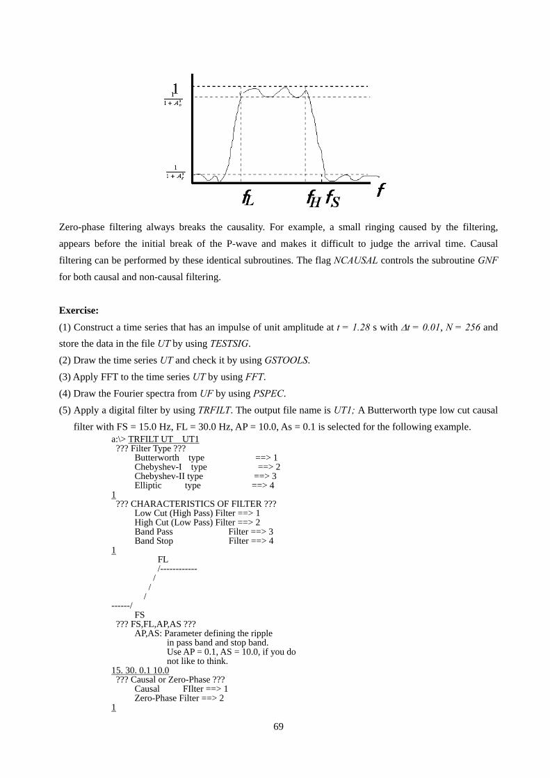
69
Zero-phase filtering always breaks the causality. For example, a small ringing caused by the filtering, appears before the initial break of the P-wave and makes it difficult to judge the arrival time. Causal filtering can be performed by these identical subroutines. The flag NCAUSAL controls the subroutine GNF for both causal and non-causal filtering.
Exercise:
(1) Construct a time series that has an impulse of unit amplitude at t = 1.28 s with Δt = 0.01, N = 256 and store the data in the file UT by using TESTSIG. (2) Draw the time series UT and check it by using GSTOOLS. (3) Apply FFT to the time series UT by using FFT. (4) Draw the Fourier spectra from UF by using PSPEC. (5) Apply a digital filter by using TRFILT. The output file name is UT1; A Butterworth type low cut causal
filter with FS = 15.0 Hz, FL = 30.0 Hz, AP = 10.0, As = 0.1 is selected for the following example. a:\> TRFILT UT UT1 ??? Filter Type ??? Butterworth type ==> 1 Chebyshev-I type ==> 2 Chebyshev-II type ==> 3 Elliptic type ==> 4 1 ??? CHARACTERISTICS OF FILTER ??? Low Cut (High Pass) Filter ==> 1 High Cut (Low Pass) Filter ==> 2 Band Pass Filter ==> 3 Band Stop Filter ==> 4 1 FL /------------ / / / ------/ FS ??? FS,FL,AP,AS ??? AP,AS: Parameter defining the ripple in pass band and stop band. Use AP = 0.1, AS = 10.0, if you do not like to think. 15. 30. 0.1 10.0 ??? Causal or Zero-Phase ??? Causal FIlter ==> 1 Zero-Phase Filter ==> 2 1

70
Fig. 50 Examples of the performance of the recursive filter designed by TRFILT.EXE. Left: the input signal that is an impulse of unit amplitude located at t = 1.28 s. Center: the output from the causal Butterworth low pass filter. Right: the output from the zero phase Butterworth low
pass filter. The parameters used are Δt = 0.01, N = 256, FS = 15.0 Hz, FL = 30.0 Hz, Ap = 0.1, As = 10.0.
(6) Draw the filtered time series UT1 by using PTIME. (7) Apply FFT to the filtered time series UT1 and store the result in the file UF1. (8) Draw the Fourier spectra stored in UF1 by using PSPEC and compare it with the drawn UF.
(9) Check the performance for filters of other types by repeating the above procedure with different values of control parameters.

71
3.5. Deconvolution or Inverse Filtering Every observed seismic waveform data is an output from some filters. For example, the
seismometer itself is a high pass filter. Amplifiers, sometimes, have frequency characteristics that are not uniform for all frequencies. Moreover, we use other high cut filter to suppress AC noise that has energy at 50 or 60 Hz since these distort seismic signals. Moreover, an anti-aliasing filter is used in digital data acquisition systems. Since seismometry is conducted not only for obtaining travel time data but also for obtaining waveform data, i. e., ground motion, we must compensate this distortion in order to obtain true ground motion. Remember that recorded signals are obtained by the convolution of the instrumental characteristics to the ground motion in the time domain and are given by their product in the frequency domain. The instrumental characteristics are identical to the response of instruments to an impulsive signal (Fig. 51 top).
( ) ( ) ( )( ) ( ) ( ).
,*ωωω GFR
tgtftr=
= (36)
where r(t), f(t), and g(t) denote the recorded signals, the instrumental response, and the ground motion in
the time domain, respectively; R(ω), F(ω), and G(ω), respectively, are the same parameters in the frequency domain.
Deconvolution in seismology is usually the process for eliminating the effect of the instrumental characteristics from the observed data and to recover the true ground motion. Mathematically, this is the reverse process of convolution. Deconvolution in the time domain corresponds to the quotient in the frequency domain. In comparison with the complexity of deconvolution in the time domain, the frequency domain operation is composed of only three steps. These are for applying the FFT to the instrument response and recorded signal, to divide the recorded signal spectra by the instrumental response spectra, and to apply the inverse FFT to the quotient (Fig. 51 middle).
( ) ( ){ } ( ).1 ωωω RFG ⋅= − (37)
However, we must consider the following. The information once lost in the observation or processing can never be recovered by any technique, even by extremely sophisticated and efficient ones. This is because we cannot avoid noises that are recorded simultaneously with the signal or those that invade into the record during the processing. Once the signals weaken and become smaller than the noise level, any recovery process only amplifies such noises. Such amplified noises can be dominant in the recovered ground motion. The signals weaken a little either only during the recording or the processing can be strengthened or recovered by the deconvolution technique.
Typically, true ground motion has band limited feature at the far field and low pass feature at the near field, whereas the ground noise is present at every frequency. Let us handle only far field ground
motion in order to have a simple demonstration. , G(ω) is band limited. The instrumental response F(ω) is also band limited, because a seismometer is a low cut filter and used with a high cut anti-alias filter. The
recovering operator in the frequency domain {F(ω)}–1 has a large amplitude at a frequency outside this limited frequency band. The recorded signal R(ω) is almost band limited but it has little energy outside the frequency band of G(ω), i.e., the contribution of the noise. By applying the inverse filter, i.e., the recovering operator {F(ω)}–1, this small contribution of the noise will be considerably amplified and

72
contaminates the recovered ground motion transformed into the time domain by the inverse FFT (Fig. 51 bottom).
This shows that we have to select a frequency range such that the signal is sufficiently larger than the noise in order to prevent instability due to the application of the inverse filter. We cannot recover the ground motion outside this frequency band.
However, the recommended method is to handle the data only within the pass band of the instrumental response. Usually, this is given by the natural frequency of the seismometer and the cutoff frequency of the anti-alias filter. It is possible but not easy to use the information outside of this range. Even within this frequency range, the above mentioned instability problem can take place due to the
smaller frequency band of G(ω). Thus, it is also recommended that the shape of R(ω) be observed and the useful frequency band be selected before beginning the data processing.
Fig. 51 Schematic illustration of Eq. (36) (top), theoretical inverse filtering process given by Eq. (37) (middle) and actual inverse filtering process with noise (bottom). Reproduced based on Sherbaum (1996).

73
Example: Inverse Filter for a Simple Moving Coil Type Seismometer The transfer function that gives the inverse response to the previous examples is given as follows:
( ) .,2
0
03
200
21
s
s
RRRGG
sshsGsT
+=
++⋅= − ωω
(36)
Fig. 52 shows the amplitude response of this transfer function.
The solutions of the equation, i.e., the numerator is equal to zero, are ( )120 −±−= hhs ω . This gives the
zero position at
( )200 1, hh −− ωω , ( )2
00 1, hh −−− ωω , for h < 1.0, the under-damped case,
( ).0,0ω− doubled for h = 1.0, critically damped case,
( )( ).0,120 −−− hhω , ( )( ).0,12
0 −+− hhω for h > 1.0, over-damped case.
The denominator, however, gives a tripled pole at (0, 0). By using the warped frequency, the transfer function is given approximately as follows.
( ) ,33
22
110
33
22
110
−−−
−−−
++++++
=zbzbzbbzazazaasT
where
( ) ( ) ( ){ }( ) ( ) ( ){ }( ) ( ) ( ){ }( ) ( ) ( ){ }
.,3,3,2tan2tan212
,2tan32tan212
,2tan32tan212
,2tan2tan212
3210
02
03
02
02
02
01
02
00
GbGbGbGbtthta
tthta
tthta
tthta
−==−==Δ+Δ−⋅Δ=
Δ+Δ−−⋅Δ=
Δ+Δ+−⋅Δ=
Δ+Δ+⋅Δ=
ωω
ωω
ωω
ωω
Since a simple moving coil type seismometer is a low cut filter, its inverse filter makes the component grow in a frequency range that is lower than the natural frequency of the seismometer. This causes an instability in the output from the filter, because the signal to noise ratio is small at this frequency range. Fig. 52 Amplitude response of the inverse filter for the voltage change between two output terminals of a simple moving coil type seismometer that is calculated by Eq. (36). The parameters used are T0 = 0.5, h = 0.71. Theoretically, this filter can convert the output voltage variation with the ground displacement. However, this amplifies the low frequency components considerably as shown clearly in this figure.
Inverse Filter for Output Voltage
0.001
0.01
0.1
1
10
100
1000
0.1 1 10 100
Frequency
Am
plitude
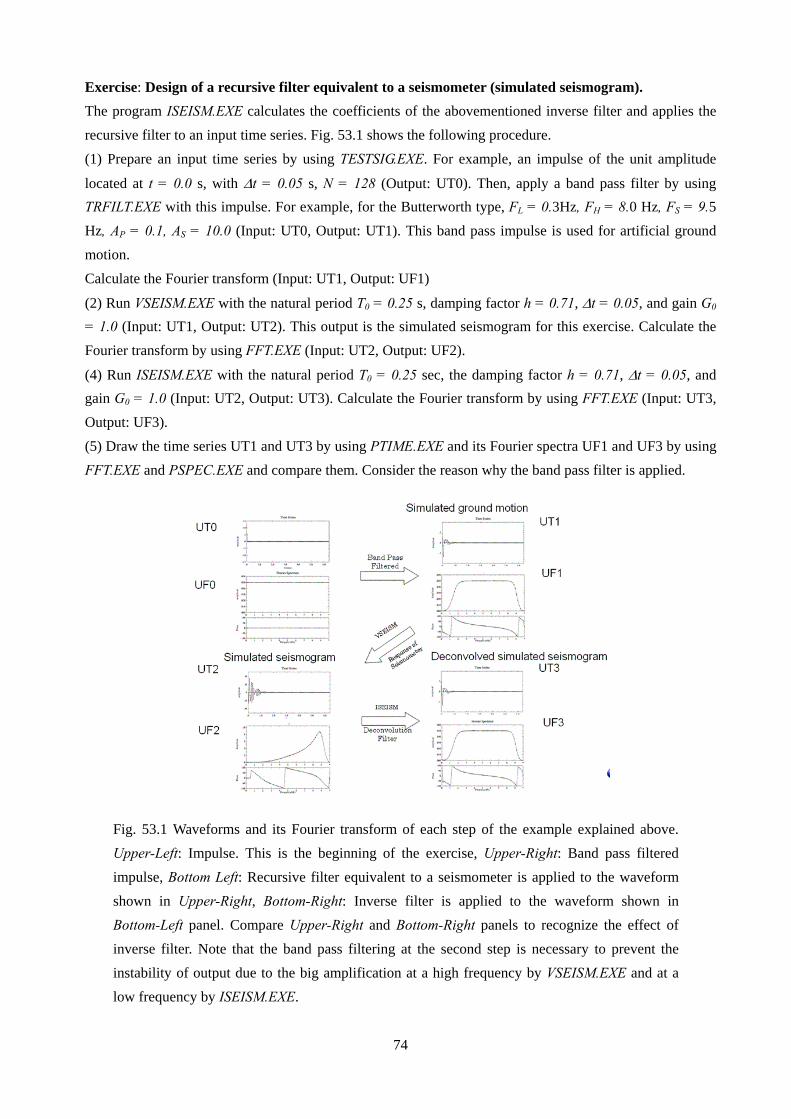
74
Exercise: Design of a recursive filter equivalent to a seismometer (simulated seismogram). The program ISEISM.EXE calculates the coefficients of the abovementioned inverse filter and applies the recursive filter to an input time series. Fig. 53.1 shows the following procedure. (1) Prepare an input time series by using TESTSIG.EXE. For example, an impulse of the unit amplitude
located at t = 0.0 s, with Δt = 0.05 s, N = 128 (Output: UT0). Then, apply a band pass filter by using TRFILT.EXE with this impulse. For example, for the Butterworth type, FL = 0.3Hz, FH = 8.0 Hz, FS = 9.5 Hz, AP = 0.1, AS = 10.0 (Input: UT0, Output: UT1). This band pass impulse is used for artificial ground motion. Calculate the Fourier transform (Input: UT1, Output: UF1)
(2) Run VSEISM.EXE with the natural period T0 = 0.25 s, damping factor h = 0.71, Δt = 0.05, and gain G0 = 1.0 (Input: UT1, Output: UT2). This output is the simulated seismogram for this exercise. Calculate the Fourier transform by using FFT.EXE (Input: UT2, Output: UF2).
(4) Run ISEISM.EXE with the natural period T0 = 0.25 sec, the damping factor h = 0.71, Δt = 0.05, and gain G0 = 1.0 (Input: UT2, Output: UT3). Calculate the Fourier transform by using FFT.EXE (Input: UT3, Output: UF3). (5) Draw the time series UT1 and UT3 by using PTIME.EXE and its Fourier spectra UF1 and UF3 by using FFT.EXE and PSPEC.EXE and compare them. Consider the reason why the band pass filter is applied.
Fig. 53.1 Waveforms and its Fourier transform of each step of the example explained above. Upper-Left: Impulse. This is the beginning of the exercise, Upper-Right: Band pass filtered impulse, Bottom Left: Recursive filter equivalent to a seismometer is applied to the waveform shown in Upper-Right, Bottom-Right: Inverse filter is applied to the waveform shown in Bottom-Left panel. Compare Upper-Right and Bottom-Right panels to recognize the effect of inverse filter. Note that the band pass filtering at the second step is necessary to prevent the instability of output due to the big amplification at a high frequency by VSEISM.EXE and at a low frequency by ISEISM.EXE.

75
Exercise: Inverse Filter for a Simple Moving Coil Type Seismometer—II (Real Seismogram) Ch1.dat is a seismogram (NS-component) observed by the L4C seismometer, the parameters of which are
Δt = 0.05, N = 8192, T0 = 1.0 s, h =0.64. (1) Draw wave forms of ch1.dat using PTIME.EXE.
(2) Run ISEISM.EXE with T0 = 1.0 s, h = 0.64, Δt = 0.02 and gain G0 = 2.7 (V/cm/s) (Input: ch1.dat, Output: UT0). (3) Apply a band pass filter by using TRFILT.EXE to this impulse. For example, the Butterworth type, FL = 0.1 Hz, FH = 18.0 Hz, FS=20.0 Hz, AP = 0.1, AS = 10.0 (Input: CH1.dat, Output: UT).
(4) Run ISEISM.EXE with T0 = 1.0 s, h = 0.64, Δt = 0.02 and gain G0 = 2.7 (V/cm/s) (Input: UT, Output: UT1). (5) Apply a band pass filter by using TRFILT.EXE with the Butterworth type, FL = 0.1 Hz, FH = 18.0 Hz, FS = 20.0 Hz, AP = 0.1, AS = 10.0 (Input: UT1, Output: UT2).
Fig. 53.2 Procedure and output of the example for a real seismogram.

76
Example: Filter for Conversion of Seismogram obtained by a Simple Moving Coil Type Seismometer to that of Longer Period Seismometer.
A simple way to avoid the abovementioned problem is to convert the system response with a longer-period seismometer.
Suppose that the damping constant and natural angular frequency of the seismometer used for
the observations are h0, ω0, then its response is
( )
( ) ( ).
21 2000
0 ωωωωω
−−⋅=
ihiGy
em
m
Let us convert this with the response from a seismometer, in which the damping constant and natural
angular frequency are h1, ω1 . ( )
( ) ( ).
21 2111
1 ωωωωω
−−⋅=
ihiGy
em
m
The inverse function in the frequency domain is
( ) ( )( ) ( )
.,2121
102111
20001 GGG
ihihG =
−−−−
⋅−
ωωωωωωωω
The transfer function in the s-domain is given as follows:
( ) .22
2111
2
2000
21
ωωωω
++++
⋅= −
shsshsGsT (37)
Then, using the warped frequency gives
( )( ) ( )( ) ( )
( ) ( )( ) ( )
,
12
tan112
tan21
12
tan112
tan21
22
110
22
110
21121111
21
21021100
21
1
−−
−−
−−−−
−−−−
−
++++
=
+⎟⎠⎞
⎜⎝⎛ Δ
++−⎟⎠⎞
⎜⎝⎛ Δ
+−
+⎟⎠⎞
⎜⎝⎛ Δ
++−⎟⎠⎞
⎜⎝⎛ Δ
+−⋅=
zbzbbzazaa
ztzzthz
ztzzthzGsT
ωω
ωω
where
( ) ( )( )( ) ( )
( ) ( ){ }( ){ }
( ) ( )( ).2tan2tan21
,2tan22
,2tan2tan21
,2tan2tan21
,2tan22
,2tan2tan21
12
112
12
1
12
110
02
002
02
1
02
000
tthGb
tGb
tthGb
ttha
ta
ttha
Δ+Δ+=
Δ+−=
Δ+Δ+=
Δ+Δ−=
Δ+−=
Δ+Δ+=
ωω
ω
ωω
ωω
ω
ωω

77
Fig. 54 Amplitude spectra of the correction filter explained above.
0.001
0.01
0.1
1
10
100
0.01 0.1 1 10 100
Frequency
Am
plitude
Original Seismometer Simulated Seismometer Correction Filter

78
Exercise: Filter for Conversion of Seismogram obtained by a Simple Moving Coil Type Seismometer to that of Longer Period Seismometer (An Impulse). (1) The program CSEISM.EXE calculates the coefficients of the recursive filter that can convert the
characteristics of the simple moving coil type seismometer used originally for (1) observing those of the simulated seismometer with a longer period.
(2) Prepare an input time series by using TESTSIG.EXE. For example, an impulse of unit amplitude located
at t = 0.0 s, with Δt =0.05 s, N = 128 (Output: UT0) (3) Calculate Fourier transform by using FFT.EXE (Input: UT0, Output: UF0).
(4) Run DSEISM.EXE with the natural period T0 = 0.25 s, the damping factor h0 = 0.71, Δt = 0.05 and the gain G0 = 1.0 (Input: UT0, Output: UT1). Calculate Fourier transform by using FFT.EXE (Input: UT1, Output: UF1).
(5) Run CSEISM.EXE with T0 = 0.25 s, h0 = 0.71, T1 = 1.0 s, h1 = 0.71, Δt = 0.05, and gain G0 = 1.0 (Input: UT1, Output: UT2). Calculate Fourier transform by using FFT.EXE (Input: UT2, Output: UF2).
Fig. 55.1 Waveforms and spectra of the example mentioned above. Left: Impulse used as the input. Center: Simulated output for a seismometer T0 = 0.25 s, h0 = 0.71 by DSEISM.EXE. Right: Converted output from T0 = 0.25, h0 = 0.71 s to T0 = 1.0, h0 = 0.71 s by CSEISMO.EXE.

79
Exercise: Filter for Conversion of Seismogram obtained by a Simple Moving Coil Type Seismometer to that of Longer Period Seismometer (Real Seismogram)
Ch1.dat is a seismogram (NS-component) observed by L4C seismometer, the parameters of which are Δt = 0.05, N = 8192, T0 = 1.0 s, h = 0.64. (1) Draw wave forms of ch1.dat using PTIME.EXE. (2) Run CSEISM.EXE with Original Seismometer T0,h,dt,g0: 1.0, 0.64, 0.02, and 2.7 (V/cm/s) Simulated Seismometer T0,h,dt,g0: 5.0, 0.71, 0.02, and 50.0 (V/cm/s) (Input: ch1.dat, Output: output.dat). Calculate Fourier transform by using FFT.EXE (Input: output.dat, Output:output.spc).
Fig. 55.2 Input signal (left): Ch1.dat and output signal (right) of CSEISMO.EXE
����� Output.dat Input.dat

80
3.6. Integration of accelerogram or Base Line Correction 3.6.1 Origin of Low-Frequency Errors Chiu (1997) explains the origins of low-frequency errors in the following manner. We are interested mainly in low-frequency noises because the effects of high-frequency noises are considerably reduced by double integration since their frequency band is lower than Nyquist frequency. (1) Deviations of the instrument response from flat amplitude response and from linear phase shift. These are large in a high-frequency range. Careful calibration by the manufacturer is essential. (2) Limited resolution of analog-to-digital Converter. This causes the approximations and the drift. (3) Insufficient sampling rate that can be prevented by considering the Nyquist frequency. Although the frequency band of interest to engineering seismologists is lower than 10 Hz, sampling with at least 100 Hz is recommended in order to obtain the value of the peak acceleration correctly. (4) Electronic Noise: besides the AC noise at 50 or 60 Hz, low-frequency electric noise caused by fluctuation of temperature is present. (5) Ambient noises that include a long-period microtremor and slow deformation of observatory building, e. g. , due to sunshine affects the integrated displacement seismogram significantly. Their effects appear superposed over each other and the seismic signals in the seismograms and in the output of digital data processing. It is almost impossible to separate the signal from these noises in the time domain. These cause the base line drift of accelerograms and absurd waveforms of velocity and displacement seismograms obtained by numerical integration. An example is shown below. Fig. 56.1 shows the original accelerograms obtained at K-NET maintained by NIED, Japan; its station is KGS005 in the northwest part of Kagoshima pref. and the seismic event (MJMA = 3.6) took place 21:26 on March 27, 1997. This is one of the aftershocks of Kagoshima-Ken Hokusei-bu Eq. (M = 6.3). These include the noises mentioned above, although there is no visible noise in the shown scale.
The acceleration amplitude spectra of the seismic event (time window; [12.0 s, 24.0 s]) shown in the top panels of Fig. 56.2 has a wide peak that corresponds to the seismic signals and a portion of noise that is more clearly shown in the low frequency band. The latter is emphasized in the displacement amplitude spectra shown in the bottom panels. Fig. 56.3 shows the amplitude spectra of the noise (time window; [0.0 s, 10.0 s]) recorded before the P-wave arrivals. A comparison of Fig. 56.3 with Fig. 56.2 shows the effects of the low-frequency noises in the frequency domain.

81
Fig. 56.1 Original Accelerograms. Plotted by pltacc.exe.
Fig. 56.2 Amplitude spectra of accelerograms shown in Fig. 56.1 for the time window [12.0 s, 24.0 s] that include the seismic event. The increasing peak at the frequency band lower than 0.4Hz is emphasized in the displacement amplitude spectra obtained by the division of
acceleration spectra by (2πf)2. Plotted by splot.exe.
82
Fig. 56.3 Amplitude spectra of accelerograms shown in Fig. 56.1 for the time window [0.0 s, 10.0 s] that is the noise part. The increasing peak at the frequency band lower than 0.4 Hz is emphasized in the displacement amplitude spectra obtained by the division of acceleration
spectra by (2πf)2 . Plotted by splot.exe. The integration of the time series can be performed by recursive filtering as given by the following.
.1 mmm xtyy ⋅Δ+= −
The velocity seismograms obtained by a direct integration of the accelerograms shown in Fig.
56.1 are shown in Fig. 56.4. These almost linearly increasing velocity seismograms show the effect of the constant offset included in the original accelerograms. The slightly observable curvature is due to the linear trend included in them.
The correction for the constant offset and linear trend in accelerograms is performed by the least
square fitting as shown by Eq. (8). Then, the numerical integration is performed. The result is shown in Fig. 56.5. This is considerably improved in comparison with Fig. 56.4. The slight base line drift of the long period is supposed to be due to the influence of the low-frequency noise remaining in the corrected accelerograms.

83
Fig. 56.4 Velocity seismograms obtained by a direct integration of the accelerograms shown in Fig. 56.1. The apparent linear trends are due to the influence of the constant drift in the accelerograms. Calculated by acc2vel.exe with comments for the offset-trend correction and band pass filtering, and then plotted by pltvel.exe.
Fig. 56.5 The accelerograms shown in Fig. 56.1 are corrected by the least square fitting method and then integrated numerically. The slight drift in the base line is due to the influence of the low-frequency noise remaining in the corrected accelerograms. Calculated by acc2vel.exe with comments due to band pass filtering, and then plotted by pltvel.exe.

84
The remaining low-frequency noises can be removed by applying the high pass or band pass filter aimed to cut the low frequency component. The example is shown in Fig. 56.6. The used values for the parameters of the band pass filter are as follows:.
fl, fh, fs/0.7, 25.0, 30.0/ ntype,nchara,ncausal/1,3,2/
fl = 0.7 Hz corresponds to the limit frequency in which the seismic signals become dominant in comparison with noises (Fig. 56.2 top panels). fh = 25.0 Hz and fs = 30.0 Hz are selected in order to ensure the suppression of high-frequency noises. Ntype = 1 means Butterworth filter and nchara = 3 means band pass feature. ncause= 2 that means that a zero-phase filter is selected in order to maintain the waveform of seismic signals.
Fig. 56.6 The accelerograms shown in Fig. 56.1 are corrected by the least square fitting method, band pass filtered, and then integrated numerically. They were calculated by acc2vel.exe and plotted by pltvel.exe.
.

85
The conversion of the accelerogram to the displacement seismogram is tougher than that in the case of a velocity seismogram because of the double integrations. Fig. 56.7 shows the result of a direct integration of the velocity seismograms shown in Fig. 56.4, i. e., those of the double direct integration of the accelerograms shown in Fig. 56.1. The parabolic feature is due to the integration of the almost linear velocity seismograms (Fig. 56.4). Note the absurdly big values of the maximum value.
.
Fig. 56.7 Displacement seismogram obtained by a direct integration of the velocity seismograms shown in Fig. 56.4. Calculated by acc2dis.exe with comments on the offset-drift correction and band pass filtering for accelerograms and velocity seismograms; subsequently plotted by pltdis.exe.

86
Fig. 56.8 shows the displacement seismogram obtained by the least square correction and the integration of the velocity seismograms shown in Fig. 56.5. These show parabolic waveforms that are integrated low-frequency noises as well. Fig. 56.9 Displacement seismogram obtained by a direct integration of the velocity seismograms shown in Fig. 56.6. Fig. 56.10 Displacement seismogram obtained by the least square correction of the velocity seismograms shown in Fig. 56.6. This give a better performance than the others, but not sufficient. A slight trend is obvious in the NS component.
Fig. 56.8 Displacement seismogram obtained by the least square correction and integration of the velocity seismograms shown in Fig. 56.5. Calculated by acc2dis.exe with comments from the band pass filtering for accelerograms and velocity seismograms; subsequently plotted by pltdis.exe.

87
Fig. 56.9 Displacement seismogram obtained by a direct integration of the velocity seismograms shown in Fig. 56.6. Calculated by acc2dis.exe with comments from the offset-drift correction and band pass filtering for velocity seismograms; subsequently plotted by pltdis.exe.
Fig. 56.10 Displacement seismogram obtained by the least square correction of the velocity seismograms shown in Fig. 56.6. Calculated by acc2dis.exe with comments from band pass filtering for velocity seismograms; subsequently plotted by pltdis.exe.

88
The attempts described above imply the necessity of an offset-drift correction and band pass filtering for accelerograms and velocity seismograms. Fig. 57.1 and Fig. 57.2 show stable results, i. e., displacement seismograms without a base line drift.
The difference between Fig. 57.1 and Fig. 57.2 is the value of the parameter fl. In Fig. 57.1, fl = 0.1 Hz, and in Fig. 57.2 fl = 0.7 Hz. A ong-period ripple is observed before P-arrival in Fig. 57.1 due to the low-frequency noises that can be suppressed by selecting fl = 0.7 Hz
The base line correction of the velocity and displacement seismograms integrated from observed an accelerogram is a very basic task for strong motion observation. The techniques of digital data processing described in this lecture note are necessary in totality.
The recommended way of integration is as follows. (1) Calculate and plot the Fourier spectra of the observed accelerogram for both noise part and seismic
event part. (2) Determine the value of fl that is the low frequency limit of the band such that the seismic signal is
dominant in comparison with the noise level. (3) Select the values of fh and fs, if the band pass filter is used. If a high pass filter is used, they are not
necessary. (4) Apply the offset-trend correction by the least square method and filtering to the observed
accelerograms. (5) Integrate the processed accelerograms; then the velocity seismograms are then obtained. (6) Apply the offset-trend correction by the least square method and filtering to the obtained velocity
seismograms. (7) Integrate the processed velocity seismograms; then the displacement seismograms are obtained. (8) If the obtained displacement seismograms have a long-period deviation before P-arrival time, return to
(2) and change the value of fl. The result can be affected by the types of filter applied. Try to check the performance of various filters on your own.

89
Fig. 57.1 Displacement seismogram obtained by the least square correction and band pass filtering of the velocity seismograms shown in Fig. 56.6. Long-period ripple observed before P-arrival is due to the low-frequency noises.
Fig. 57.2 Displacement seismogram obtained by the least square correction and band pass filtering of the velocity seismograms shown in Fig. 56.6. Long-period ripple observed before P-arrival in Fig. 57.1 is suppressed sufficiently.
90
Fortran Programs
CFFT.FOR c******************************************************** SUBROUTINE CFFT(X,N,IND) c........................................................................... c Complex Fast Fourier Transform c Coded by Y. OHSAKI in "Introduction to spectral analysis for c seismic waves" c Typed by D.Suetsugu, IISEE c Modified by H.Inoue, IISEE c Usage....... CALL FFT(N,X,IND) c where c X(N) In/Out Equi-spaced N complex data/Transformed values c N In Number of data, MUST be a power of 2. c IND In -1=Fourier transform, 1=Inverse Fourier transform c c Note..... You must divide the output X() by N to get Fourier c transform when IND=-1. c........................................................................... complex x(n),temp,theta c j=1 do 140 i=1,n if(i.ge.j) goto 110 temp=x(j) x(j)=x(i) x(i)=temp 110 m=n/2 120 if(j.le.m) goto 130 j=j-m m=m/2 if(m.ge.2) goto 120 130 j=j+m 140 continue c kmax=1 do 150 kkk=1,9999 if(kmax.ge.n) return istep=kmax*2 do 170 k=1,kmax theta=cmplx(0.0,3.141593*float(ind*(k-1))/float(kmax)) do 160 i=k,n,istep j=i+kmax temp=x(j)*cexp(theta) x(j)=x(i)-temp x(i)=x(i)+temp 160 continue 170 continue kmax=istep 150 continue end
TESTSIG.FOR c******************************************************** c Make a test signal u(t) c******************************************************** program main parameter (nmax=8192,pi=3.1415926536) real t(nmax),u(nmax) character yn*1,ofile*80 c if(nargs().le.1) then write(*,*) write(*,*) 'Usage: TESTSIG outfile' stop ' ' end if call getarg(1,ofile,istatus) c .......................................... Input parameters write(*,*) write(*,*) 'Parameters for a test signal.' write(*,'(a$)') ' Sampling interval dT (sec) >>' read(*,*) dt write(*,'(a$)') ' Number of data points N >>' read(*,*) ndata write(*,'(1x,a,f10.3,a)')'Total time is',dt*ndata,' sec.' write(*,'(1x,72a)') ('-',i=1,72) do i=1,ndata t(i)=(i-1)*dt u(i)=0.0 end do c ......................................... Superposition loop do isum=1,999 write(*,'(a$)') ' Cos/Sin=1, Const=2, Impulse=3,'// & ' Step=4, Triangle=5, Square=6 >>' read(*,*) ichoice if(ichoice.eq.1) then write(*,'(a$)') ' Period of the cosine wave (sec)>>'
read(*,*) period write(*,'(a$)') ' Amplitude >>' read(*,*) amp write(*,'(a$)') ' Phase (0-360 in degree) >>' read(*,*) phase write(*,'(a$)') ' Damping factor >>' read(*,*) damp do i=1,ndata arg=phase/180.*pi+2*pi/period*t(i) u(i)=u(i)+amp*cos(arg)*exp(-damp*t(i)) end do else if(ichoice.eq.2) then write(*,'(a$)') ' The constant value >>' read(*,*) const do i=1,ndata u(i)=u(i)+const end do else if(ichoice.eq.3) then write(*,'(a$)') ' Location of the impulse (sec) >>' read(*,*) timpulse write(*,'(a$)') ' Amplitude of the impulse >>' read(*,*) aimpulse do i=1,ndata if(t(i).ge.timpulse) then u(i)=u(i)+aimpulse exit end if end do else if(ichoice.eq.4) then write(*,'(a$)') ' Location of the step(sec) >>' read(*,*) tstep write(*,'(a$)') ' Amplitude of the step >>' read(*,*) astep do i=1,ndata if(t(i).ge.tstep) then u(i)=u(i)+astep end if end do else if(ichoice.eq.5) then write(*,'(a$)')'Period of the triangular wave(sec)>>' read(*,*) period write(*,'(a$)') ' Amplitude >>' read(*,*) amp write(*,'(a$)') ' Phase (0-360 in degree) >>' read(*,*) phase do i=1,ndata half=period/2. tt=t(i)+phase/360.*period tmod=mod(tt,half) if(mod(int(tt/half),2).eq.0) then u(i)=u(i)+amp-amp*2*tmod/half else u(i)=u(i)-amp+amp*2*tmod/half end if end do else if(ichoice.eq.6) then write(*,'(a$)')'Period of the square wave(sec) >>' read(*,*) period write(*,'(a$)') ' Amplitude >>' read(*,*) amp write(*,'(a$)') ' Phase (0-360 in degree) >>' read(*,*) phase do i=1,ndata half=period/2 tt=t(i)+phase/360*period+period/4.0 if(mod(int(tt/half),2).eq.0) then u(i)=u(i)+amp else u(i)=u(i)-amp end if end do end if write(*,'(a$)') ' Add more? (y/n) >>' read(*,'(a)') yn if(yn.ne.'y'.and.yn.ne.'Y') exit end do write(*,'(1x,72a)') ('-',i=1,72) c ............................... Output Time Series open(10,file=ofile) write(10,*) ndata,' =N' write(10,*) dt,' =dT (sec)' do i=1,ndata write(10,*) u(i) end do close(10) write(*,*) 'Done' c end

91
PTIME.FOR c******************************************************** c Plot time series in a file c******************************************************** program main parameter (nmax=8192) real t(nmax),u(nmax) character ifile*80 c ............................... ........ Input Time Series if(nargs().le.1) then write(*,*) write(*,*) 'Usage: PTIME infile' stop ' ' end if call getarg(1,ifile,istatus) open(10,file=ifile,status='old') read(10,*) ndata read(10,*) dt do i=1,ndata read(10,*) u(i) t(i)=dt*(i-1) end do close(10) c ............................... Plot Time Series umax=u(1) umin=u(1) do i=2,ndata if(u(i).gt.umax) umax=u(i) if(u(i).lt.umin) umin=u(i) end do ymax=max(abs(umax),abs(umin))*1.5 c call opengraphics call setwindow(1,0.,-ymax,dt*ndata,ymax) call setviewpt(1,0.3,0.3,1.1,0.7) call drawtitle('Time Series') cc call setline('width=2') call settext('size=0.8') call drawaxis('labelx=Time(s),labely=Amplitude') call drawline(0.,0.,dt*ndata,0.) call setmark('type=solid-square,size=0.5') call drawlines(ndata,t,u) call drawmarks(ndata,t,u) call closegraphics end
FFT.FOR include 'cfft.for' c******************************************************** c Calculate Fourier Coefficients by FFT c******************************************************** parameter(nmax=8192) real u(nmax) complex cf(nmax) character ifile*80,ofile*80 c if(nargs().le.2) then write(*,*) write(*,*) 'Usage: FFT infile outfile' stop ' ' end if call getarg(1,ifile,istatus) call getarg(2,ofile,istatus) c.......................................... Read time series from file open(10,file=ifile,status='old') read(10,*) ndata read(10,*) dt do i=1,ndata read(10,*) u(i) end do close(10) c............................................ Check if ndata=2**n npow=nint(log(float(ndata))/log(2.0)) nn=2**npow if(ndata.ne.nn) then write(*,*) 'N=',ndata,', Error: N must be a power of 2.' stop end if c........................................................... FFT do i=1,nn cf(i)=cmplx(u(i),0.0) end do call cfft(cf,nn,-1) do i=1,nn cf(i)=cf(i)/nn end do c.................................... Write Fourier Coeff. to file df=1.0/(dt*nn) open(20,file=ofile) write(20,*) nn,' =N'
write(20,*) df,' =df' do i=1,nn write(20,*) cf(i) end do close(20) write(*,*) 'Done' c............................................................. end
PCFFT.FOR c******************************************************** c Plot FFT Coefficients c******************************************************** character*20 ifile,ofile parameter(nmax=8192,pi=3.1415926535,d2r=pi/180.) complex cf(nmax) real amp(nmax/2),phase(nmax/2),freq(nmax/2) c..................................................Input from file if(nargs().le.1) then write(*,*) write(*,*) 'Usage: PFFT infile' stop ' ' end if call getarg(1,ifile,istatus) open(10,file=ifile,status='old') read(10,*) nn read(10,*) df do i=1,nn read(10,*) cf(i) end do close(10) fmax=nn/2*df c................................................ Plot spectrum i=0 do k=nn/2+1,nn-1 i=i+1 freq(i)=(k-nn)*df amp(i)=cabs(cf(k+1)) if(amp(i).ne.0.0) then phase(i)=atan2(imag(cf(k+1)),real(cf(k+1)))/d2r end if end do do k=0,nn/2 i=i+1 freq(i)=df*k amp(i)=cabs(cf(k+1)) if(amp(i).ne.0.0) then phase(i)=atan2(imag(cf(k+1)),real(cf(k+1)))/d2r end if end do c ampmax=amp(1) do i=2,nn if(amp(i).gt.ampmax) ampmax=amp(i) end do do i=1,nn if(amp(i)/ampmax.lt.1.e-5) then phase(i)=0.0 end if end do c c........................................................ Graphics call opengraphics call setwindow(1,-fmax,0.0,fmax,ampmax*1.2) call setviewpt(1,0.3,0.45,1.1,0.8) call drawtitle('FFT Coefficients') call settext('size=0.8') call drawaxis('labely=Amplitude') call setwindow(2,-fmax,-180.,fmax,180.) call setviewpt(2,0.3,0.2,1.1,0.40) call drawaxis('labelx=Frequency(Hz),labely=Phase,'// & 'dy=90,ddy=90') c.................................... Plot amplitude and phase spectrum call setmark('type=solid-square,size=0.7') call selectwindow(1) call drawlines(nn,freq,amp) call drawmarks(nn,freq,amp) call selectwindow(2) call drawlines(nn,freq,phase) call drawmarks(nn,freq,phase) call closegraphics c............................................................. end
PSPEC.FOR c******************************************************* c Plot Fourier Spectrum c******************************************************** character*20 ifile,ofile

92
parameter(nmax=8192,pi=3.1415926535,d2r=pi/180.) complex cf(nmax) real amp(nmax/2),phase(nmax/2),freq(nmax/2) c.................................................. Input from file if(nargs().le.1) then write(*,*) write(*,*) 'Usage: PSPEC infile' stop ' ' end if call getarg(1,ifile,istatus) open(10,file=ifile,status='old') read(10,*) nn read(10,*) df do i=1,nn read(10,*) cf(i) end do close(10) c................................................ Plot spectrum do i=1,nn/2+1 freq(i)=df*(i-1) amp(i)=cabs(cf(i))/df end do fmax=nn/2*df c ampmax=amp(1) do i=2,nn/2+1 if(amp(i).gt.ampmax) ampmax=amp(i) end do do i=1,nn if(amp(i)/ampmax.gt.1.e-5) then phase(i)=atan2(imag(cf(i)),real(cf(i)))/d2r else phase(i)=0.0 end if end do c c........................................................ Graphics call opengraphics call setwindow(1,0.0,0.0,fmax,ampmax*1.2) call setviewpt(1,0.3,0.45,1.1,0.8) call drawtitle('Fourier Spectrum') call settext('size=0.8') cc call setline('width=2.0') call drawaxis('labely=Amplitude') call setwindow(2,0.0,-180.,fmax,180.) call setviewpt(2,0.3,0.2,1.1,0.40) call drawaxis('labelx=Frequency(Hz),labely=Phase,'// & 'dy=90,ddy=90') c.................................... Plot amplitude and phase spectrum call setmark('type=solid-square,size=0.5') call selectwindow(1) call drawlines(nn/2+1,freq,amp) call drawmarks(nn/2+1,freq,amp) call selectwindow(2) call drawlines(nn/2+1,freq,phase) call drawmarks(nn/2+1,freq,phase) call closegraphics c............................................................. end
IFFT.FOR include 'cfft.for' c******************************************************** c Inverse FFT c******************************************************** parameter(nmax=8192) complex cf(nmax) character ifile*80,ofile*80 c if(nargs().le.2) then write(*,*) write(*,*) 'Usage: IFFT infile outfile' stop ' ' end if call getarg(1,ifile,istatus) call getarg(2,ofile,istatus) c................................................... Read Fourier Coeff. open(10,file=ifile,status='old') read(10,*) nn read(10,*) df do i=1,nn read(10,*) cf(i) end do close(10) c............................................................. Inv FFT call cfft(cf,nn,1) c.................................................... Write time series
open(20,file=ofile) write(20,*) nn, ' =N' write(20,*) (1.0/df)/nn, ' =dt' do i=1,nn write(20,*) real(cf(i)) end do close(20) write(*,*) 'Done' c end
FFILT.FOR c******************************************************** c Designing filter in the frequency domain c******************************************************** parameter(nmax=8192) complex cf(nmax) character ofile*80 c write(6,*)'??? OUTPUT FILE NAME ???' read(5,'(a)') ofile c........................................ Input parameters write(6,*) write(6,*) 'Parameters for a filter wavelet.' write(6,'(a)') ' Sampling interval dT (sec) >>' read(5,*) dt write(6,'(a)') ' Number of data points N >>' read(5,*) ndata write(6,'(1x,a,f10.3,a)')'Total time is',dt*ndata,' sec.' write(6,'(1x,72a)') ('-',i=1,72) c............................................ Check if ndata=2**n npow=nint(log(float(ndata))/log(2.0)) nn=2**npow if(ndata.ne.nn) then write(6,*) 'N=',ndata,', Error: N must be a power of 2.' stop end if td=dt*ndata df=1./td fnyq=0.5/dt goto 78 77 continue write(6,*)'Try again!' 78 continue c........................Read filter parameter (f1,f2,f3,f4) write(6,*)' ------------\ ' write(6,*)' / \ ' write(6,*)' / \ ' write(6,*)' / \ ' write(6,*)' / \ ' write(6,*)' / \ ' write(6,*)'---- ----------' write(6,*)' f1 < f2 < f3 < f4 <',fnyq,'Hz' read(5,*) f1,f2,f3,f4 c........................ Calculate Fourier Coefficients of filter if(f4.ge.fnyq) then write(6,*)' f4 must be less than the Nyquist frequency.' goto 77 endif if(f1.ge.f2) then write(6,*)' f1 must be less than f2.' goto 77 endif if(f2.ge.f3) then write(6,*)' f2 must be less than f3.' goto 77 endif if(f3.ge.f4) then write(6,*)' f3 must be less than f4.' goto 77 endif n1=int(f1/df)+1 n2=int(f2/df+0.5) n3=int(f3/df+0.5) n4=int(f4/df) do i=1,n1 cf(i)=cmplx(0.0,0.0) end do do i=n1+1,n2 cf(i)=cmplx(real(i-n1)*df/(f2-f1)/td,0.0) enddo do i=n2+1,n3 cf(i)=cmplx(1./td,0.0) enddo do i=n3+1,n4 cf(i)=cmplx((1.0-real(i-n3)*df/(f4-f3))/td,0.0) enddo do i=n4+1,nn/2 cf(i)=cmplx(0.0,0.0) enddo

93
do i=nn/2+1,nn cf(i)=conjg(cf(nn-i+1)) enddo c.................................... Write Fourier Coeff. to file open(20,file=ofile) write(20,*) nn,' =N' write(20,*) df,' =df' do i=1,nn write(20,*) cf(i) end do close(20) write(6,*) 'It is assumed that the phase spectra are zero.' write(6,*) 'Done' c............................................................. end
FPRDCT.FOR c******************************************************** c Product of filter spectra and input time series spectra c******************************************************** character*20 ifile,ofile parameter(nmax=8192) complex cf1(nmax),cf2(nmax) c..................................................Input from file 10 write(6,*)'??? INPUT FILE NAME (FIlter Spectra) ???' read(5,'(a)') ifile open(10,file=ifile,status='old') read(10,*) nn read(10,*) df do i=1,nn read(10,*) cf1(i) end do close(10) write(6,*)'??? INPUT FILE NAME (Input Signal Spectra) ???' read(5,'(a)') ifile open(10,file=ifile,status='old') read(10,*) nn1 read(10,*) df1 do i=1,nn read(10,*) cf2(i) end do close(10) if(nn1.ne.nn.or.df1.ne.df) then write(6,*)'Data number or frequency interval unmatched.' goto 10 endif fmax=nn/2*df td=1./df c................................................ Product do i=1,nn/2 cf1(i)=cf1(i)*cf2(i)*td enddo do i=nn/2+1,nn cf1(i)=conjg(cf1(nn-i+1)) enddo c.................................... Write Fourier Coeff. to file write(6,*)'??? OUTPUT FILE NAME ???' read(5,'(a)') ofile open(20,file=ofile) write(20,*) nn,' =N' write(20,*) df,' =df' do i=1,nn write(20,*) cf1(i) end do close(20) write(6,*)'Done' end
FWVLET.FOR c******************************************************** c Make filter wavelet of a filter from the inverse c Fourier Transform of given amplitude spectra c******************************************************** program main parameter (nmax=8192) real u(nmax),wt(nmax) character ifile*80,ofile*80 c ............................... ........ Input Time Series write(6,*)'??? INPUT FILE NAME' read(5,'(a)') ifile write(6,*)'??? OUTPUT FILE NAME' read(5,'(a)') ofile open(10,file=ifile,status='old') read(10,*) ndata read(10,*) dt do i=1,ndata read(10,*) u(i) end do close(10)
c ....................................... make filter wavelet 11 write(6,*)'Causal (1) or Zero phase (2) ???' read(5,*) iflg if(iflg.eq.1) then write(6,*) *'How many points will you use for the weighted moving average?' read(5,*) np do i=1,np wt(i)=u(i) enddo else if(iflg.eq.2) then write(6,*) *'How many points will you use for the weighted moving average?', *'The number must be odd. ' read(5,*) np nph=(np-1)/2 do i=1,nph wt(i)=u(ndata-nph+i) enddo do i=nph+1,np wt(i)=u(i-nph) enddo else goto 11 endif do i=1,np write(6,*) i,wt(i) enddo open(10,file=ofile,status='unknown') write(10,*) np,iflg write(10,*) dt,' =dT (sec)' do i=1,np write(10,*) wt(i) end do close(10) end
FCONV.FOR c******************************************************** c Filtering by convolution in the time domain c******************************************************** program main parameter (nmax=8192) real wt(nmax),v(nmax),u(nmax) character*80 ifile,ofile c ............................... ........ Input Time Series write(6,*)'??? INPUT FILE NAME (Filter Wavelet)???' read(5,'(a)') ifile open(10,file=ifile,status='old') read(10,*) np,iflg read(10,*) dt do i=1,np read(10,*) wt(i) end do close(10) write(6,*)'??? INPUT FILE NAME (Input Signal)???' read(5,'(a)') ifile open(10,file=ifile,status='old') read(10,*) ndata read(10,*) dt1 if(dt1.ne.dt) then write(6,*)'Time interval unmatched!' stop endif do i=1,ndata read(10,*) u(i) end do close(10) c................................................ Convolution c Reverse filter time series c ---> Coefficient of weighted moving average if(iflg.eq.1) then write(6,*)'Causal Filtering' do n=1,np v(n)=0.0 do m=1,n v(n)=v(n)+wt(n-m)*u(m)*dt enddo enddo do n=np+1,ndata
v(n)=0.0 do m=n-np,n v(n)=v(n)+wt(n-m)*u(m)*dt enddo enddo else if(iflg.eq.2) then nph=(np-1)/2 write(6,*)'Zero phase filtering'

94
do n=1,nph v(n)=0.0 do m=1,n+nph v(n)=v(n)+wt(n-m+nph+1)*u(m)*dt enddo enddo do n=nph+1,ndata v(n)=0.0 do m=n-nph,n+nph v(n)=v(n)+wt(n-m+nph+1)*u(m)*dt enddo enddo endif c ............................... Output Time Series write(6,*)'??? OUTPUT FILE NAME ???' read(5,'(a)') ofile open(10,file=ofile,status='unknown') write(10,*) ndata,' =N' write(10,*) dt,' =dT (sec)' do i=1,ndata write(10,*) v(i) end do close(10) write(6,*) 'Done' stop end BANDP1 subroutine bandp1(x,n,dt,fl,fh,fs,ap,as,ntype,nchara,ncausal) real*4 x(n),y(65536),f(128) c write(6,*)' Filter coefficients calculation started' flu=fl*dt fhu=fh*dt fsu=fs*dt c............................................Calculation of filter coefficients if(ntype.eq.1) then c Butterworth Filter if(nchara.eq.1) then c Low-Cut (High-Pass) Filter call buthip(f,mf,gn,nchb,flu,fsu,ap,as) else if(nchara.eq.2) then c High-Cut (Low-Pass) Filter c write(6,*)' high cut' call butlop(f,mf,gn,nchb,fhu,fsu,ap,as) else if(nchara.eq.3) then c Band-Pass Filter call butpas(f,mf,gn,nchb,flu,fhu,fsu,ap,as) else c Band-Stop Filter call butstp(f,mf,gn,nchb,flu,fhu,fsu,ap,as) endif else if(ntype.eq.2) then c Chevyshev-I FIlter if(nchara.eq.1) then c Low-Cut (High-Pass) Filter call chbhip(f,mf,gn,nchb,eps,fhu,fsu,ap,as) else if(nchara.eq.2) then c High-Cut (Low-Pass) Filter call chblop(f,mf,gn,nchb,eps,flu,fsu,ap,as) else if(nchara.eq.3) then c Band-Pass Filter call chbpas(f,mf,gn,nchb,eps,flu,fhu,fsu,ap,as) else c Band-Stop Filter call chbstp(f,mf,gn,nchb,eps,flu,fhu,fsu,ap,as) endif else if(ntype.eq.3) then c Chevyshev-II FIlter if(nchara.eq.1) then c Low-Cut (High-Pass) Filter call tchhip(f,mf,gn,nchb,eps,fhu,fsu,ap,as) else if(nchara.eq.2) then c High-Cut (Low-Pass) Filter call tchlop(f,mf,gn,nchb,eps,flu,fsu,ap,as) else if(nchara.eq.3) then c Band-Pass Filter call tchpas(f,mf,gn,nchb,eps,flu,fhu,fsu,ap,as) else
c Band-Stop Filter call tchstp(f,mf,gn,nchb,eps,flu,fhu,fsu,ap,as) endif else c Elliptic Filter if(nchara.eq.1) then c Low-Cut (High-Pass) Filter call equhip(f,mf,gn,nchb,eps,ek,er,fhu,fsu,ap,as) else if(nchara.eq.2) then c High-Cut (Low-Pass) Filter call equlop(f,mf,gn,nchb,eps,ek,er,flu,fsu,ap,as) else if(nchara.eq.3) then c Band-Pass Filter call equpas(f,mf,gn,nchb,eps,ek,er,flu,fhu,fsu,ap,as) else c Band-Stop Filter call equstp(f,mf,gn,nchb,eps,ek,er,flu,fhu,fsu,ap,as) endif endif c c write(6,*)' Filter coefficients are calculated.' c write(6,'(2x,a3,i3,2x,a3,f10.6)')'mf=',mf,'gn=',gn c write(6,'(2x,i2,f10.6)') (i,f(i),i=1,mf) c..........................................................Filtering subroutine call gnf(x,y,n,f,mf,gn,ncausal) return end
TRFILT.FOR c******************************************************** c Filtering in the time domain (Recursive filter) c******************************************************** include 'rfilter.for' C program main parameter (nmax=8192) real t(nmax),u(nmax) character ifile*80,ofile*80 c....................................... Input Time Series write(6,*)'??? INPUT FILE NAME ???' read(5,'(a)') ifile write(6,*)'??? OUTPUT FILE NAME ???' read(5,'(a)') ofile open(10,file=ifile,status='old') read(10,*) ndata read(10,*) dt do i=1,ndata read(10,*) u(i) t(i)=dt*real(i-1) end do close(10) C............................................... Filtering 10 write(6,*) ' ??? Filter Type ???' write(6,*) ' Butterworth type ==> 1' write(6,*) ' Chebyshev-I type ==> 2' write(6,*) ' Chebyshev-II type ==> 3' write(6,*) ' Elliptic type ==> 4' read(5,*) ntype if(ntype.GT.4.OR.ntype.LT.1) GOTO 10 20 write(6,*) ' ??? CHARACTERISTICS OF FILTER ???' write(6,*) ' Low-Cut (High-Pass) Filter ==> 1' write(6,*) ' High-cut (Low-Pass) Filter ==> 2' write(6,*) ' Band-Pass Filter ==> 3' write(6,*) ' Band-Stop Filter ==> 4' read(5,*) nchara if(nchara.GT.4.OR.nchara.LT.1) GOTO 20 if(nchara.eq.1) then c Low-Cut (High-Pass) Filter write(6,*) ' FL ' write(6,*) ' /------------' write(6,*) ' / ' write(6,*) ' / ' write(6,*) ' / ' write(6,*) '------/ ' write(6,*) ' FS ' write(6,*) ' ??? FS,FL,AP,AS ???' write(6,*) ' AP,AS: Parameter defining the ripple ' write(6,*) ' in pass band and stop band. ' write(6,*) ' Use AP=0.1, AS=10.0, if you do' write(6,*) ' not like to think. ' read(5,*) fs,fl,ap,as else if(nchara.eq.2) then c High-Cut (Low-Pass) Filter

95
write(6,*) ' FH ' write(6,*) '------\ ' write(6,*) ' \ ' write(6,*) ' \ ' write(6,*) ' \ ' write(6,*) ' \------------' write(6,*) ' FS ' write(6,*) ' ??? FH,FS,AP,AS ???' write(6,*) ' AP,AS: Parameter defining the ripple ' write(6,*) ' in pass band and stop band. ' write(6,*) ' Use AP=0.1, AS=10.0, if you do' write(6,*) ' not like to think. ' read(5,*) fh,fs,ap,as else if(nchara.eq.3) then c Band Pass Filter write(6,*) ' FL FH ' write(6,*) ' /--------\ ' write(6,*) ' / \ ' write(6,*) ' / \ ' write(6,*) ' / \ ' write(6,*) '------/ \------' write(6,*) ' FS ' write(6,*) ' ??? FL,FH,FS,AP,AS ???' write(6,*) ' AP,AS: Parameter defining the ripple ' write(6,*) ' in pass band and stop band. ' write(6,*) ' Use AP=0.1, AS=10.0, if you do' write(6,*) ' not like to think. ' read(5,*) fl,fh,fs,ap,as else if(nchara.eq.4) then c Band Stop Filter write(6,*) ' FL FH ' write(6,*) '------\ /------------' write(6,*) ' \ / ' write(6,*) ' \ / ' write(6,*) ' \ / ' write(6,*) ' \------/ ' write(6,*) ' FS ' write(6,*) ' ??? FL,FS,FH,AP,AS ???' write(6,*) ' AP,AS: Parameter defining the ripple ' write(6,*) ' in pass band and stop band. ' write(6,*) ' Use AP=0.1, AS=10.0, if you do' write(6,*) ' not like to think. ' read(5,*) fl,fs,fh,ap,as endif c write(6,*) fl,fh,fs,ap,as write(6,*) ' ??? Causal or Zero-Phase ???' write(6,*) ' Causal FIlter ==> 1' write(6,*) ' Zero-Phase Filter ==> 2' read(5,*) ncausal call bandp1(u,ndata,dt,fl,fh,fs,ap,as,ntype,nchara,ncausal) c............................................................Output Time Series open(10,file=ofile) write(10,*) ndata,' =N' write(10,*) dt,' =dT (sec)' do i=1,ndata write(10,*) u(i) end do close(10) write(*,*) 'Done' stop end
RFILTER.FOR c******************************************************** c slave routine for trfilt.for c******************************************************** include 'buthip.f' include 'butlop.f' include 'butpas.f' include 'butstp.f' include 'chbhip.f' include 'chblop.f' include 'chbpas.f' include 'chbstp.f' include 'tchhip.f' include 'tchlop.f' include 'tchpas.f' include 'tchstp.f' include 'equhip.f' include 'equlop.f' include 'equpas.f' include 'equstp.f' include 'equpol.f' include 'celin1.f' include 'snthet.f' include 'tandem.f'
include 'recfil.f' C----------------------------------------------------------------------------. subroutine bandp(x,n,dt,fl,fh,fs,ap,as,ntype,nchara,ncausal) real*4 x(n),y(8192),f(128) c write(6,*)' Filter coefficients calculation started' flu=fl*dt fhu=fh*dt fsu=fs*dt c............................................Calculation of filter coefficients if(ntype.eq.1) then c Butterworth Filter if(nchara.eq.1) then c Low-Cut (High-Pass) Filter call buthip(f,mf,gn,nchb,flu,fsu,ap,as) else if(nchara.eq.2) then c High-Cut (Low-Pass) Filter write(6,*)' high cut' call butlop(f,mf,gn,nchb,fhu,fsu,ap,as) else if(nchara.eq.3) then c Band-Pass Filter call butpas(f,mf,gn,nchb,flu,fhu,fsu,ap,as) else c Band-Stop Filter call butstp(f,mf,gn,nchb,flu,fhu,fsu,ap,as) endif else if(ntype.eq.2) then c Chevyshev-I FIlter if(nchara.eq.1) then c Low-Cut (High-Pass) Filter call chbhip(f,mf,gn,nchb,eps,fhu,fsu,ap,as) else if(nchara.eq.2) then c High-Cut (Low-Pass) Filter call chblop(f,mf,gn,nchb,eps,flu,fsu,ap,as) else if(nchara.eq.3) then c Band-Pass Filter call chbpas(f,mf,gn,nchb,eps,flu,fhu,fsu,ap,as) else c Band-Stop Filter call chbstp(f,mf,gn,nchb,eps,flu,fhu,fsu,ap,as) endif else if(ntype.eq.3) then c Chevyshev-II FIlter if(nchara.eq.1) then c Low-Cut (High-Pass) Filter call tchhip(f,mf,gn,nchb,eps,fhu,fsu,ap,as) else if(nchara.eq.2) then c High-Cut (Low-Pass) Filter call tchlop(f,mf,gn,nchb,eps,flu,fsu,ap,as) else if(nchara.eq.3) then c Band-Pass Filter call tchpas(f,mf,gn,nchb,eps,flu,fhu,fsu,ap,as) else c Band-Stop Filter call tchstp(f,mf,gn,nchb,eps,flu,fhu,fsu,ap,as) endif else c Elliptic Filter if(nchara.eq.1) then c Low-Cut (High-Pass) Filter call equhip(f,mf,gn,nchb,eps,ek,er,fhu,fsu,ap,as) else if(nchara.eq.2) then c High-Cut (Low-Pass) Filter call equlop(f,mf,gn,nchb,eps,ek,er,flu,fsu,ap,as) else if(nchara.eq.3) then c Band-Pass Filter call equpas(f,mf,gn,nchb,eps,ek,er,flu,fhu,fsu,ap,as) else c Band-Stop Filter call equstp(f,mf,gn,nchb,eps,ek,er,flu,fhu,fsu,ap,as) endif endif c write(6,*)' Filter coefficients are calculated.' write(6,'(2x,a3,i3,2x,a3,f10.6)')'mf=',mf,'gn=',gn write(6,'(2x,i2,f10.6)') (i,f(i),i=1,mf) c..........................................................Filtering subroutine call gnf(x,y,n,f,mf,gn,ncausal) return

96
end C-----------------------------------------------------------------------------. subroutine gnf(x,y,nn,f,mf,gn,ncausal) real*4 x(nn),y(8192),f(4) if(ncausal.eq.2) then call tandem(x,y,nn,f,mf,-1) write(6,*)' TANDEM-1' do 813 i=1,nn 813 x(i)=y(i)*gn endif call tandem(x,y,nn,f,mf, 1) write(6,*)' TANDEM 1' do 815 i=1,nn 815 x(i)=y(i)*gn return end
DSEISM.FOR program dseism c******************************************************* c digital filter equivarent to displacement seismometer c******************************************************* parameter (nmax=8192) real v(nmax),u(nmax) character*80 ifile,ofile data pai/3.1415926535/ write(6,*)' Natural Period:T0, Damping Facter:h' write(6,*)' Sampling interval:dt, Gain:G0' read(5,*) t0,h,dt,g0 omg0=2.*pai/t0 write(6,*) omg0 omg0=(2./dt)*tan(omg0*dt/2.) qq=tan(omg0*dt/2.) qq2=qq*qq a0= 1.0 a1=-2.0 a2= 1.0 b0= 1.0+2.*h*qq+qq2 b1=-2.0+2.*qq2 b2= 1.0-2.*h*qq+qq2 write(6,*)' Numerator =',a0,a1,a2 write(6,*)' Denominator=',b0,b1,b2 c....................................................input write(6,*)'??? INPUT FILE NAME (Input Signal)???' read(5,'(a)') ifile open(10,file=ifile,status='old') read(10,*) ndata read(10,*) dt1 if(dt1.ne.dt) then write(6,*)'Time interval unmatched!' stop endif do i=1,ndata read(10,*) u(i) end do close(10) c............................................Recursive Filtering write(6,*)'Causal Filtering' v(1)= a0*u(1)/b0 v(2)=(a0*u(2)+a1*u(1)-b1*v(1))/b0 do i=3,ndata v(i)=(a0*u(i)+a1*u(i-1)+a2*u(i-2) * -b1*v(i-1)-b2*v(i-2))/b0 enddo c ............................... Output Time Series write(6,*)'??? OUTPUT FILE NAME ???' read(5,'(a)') ofile open(10,file=ofile,status='unknown') write(10,*) ndata,' =N' write(10,*) dt,' =dT (sec)' do i=1,ndata write(10,*) v(i) end do close(10) write(6,*) 'Done' stop end
FWARP.FOR c******************************************************** c Calculate and Plot warped angular frequency c******************************************************** program main parameter (nmax=8192) real x(nmax),y(nmax) data pai/3.1415926535/ c ............................... ........ Input
write(6,*)'??? Dt, Ndata' read(5,*) dt, ndata td=ndata*dt domg=2.*pai/td omgnyq=pai/dt do i=1,ndata x(i)=real(i-1)*domg y(i)=(2./dt)*tan(x(i)*dt/2.) end do c ............................... Plot Time Series umax=y(1) umin=y(1) do i=2,ndata if(y(i).gt.umax) umax=y(i) if(y(i).lt.umin) umin=y(i) end do cc ymax=max(abs(umax),abs(umin))*1.5 ymax=pai/dt c call opengraphics call setwindow(1,0.,0.,omgnyq*2,ymax) call setviewpt(1,0.3,0.3,1.0,0.5) call drawtitle('Warped Angular Frequency') call setline('width=2') call settext('size=0.8') call drawaxis('labelx=omg,labely=omg(k)') call drawline(omgnyq,0.,omgnyq,ymax) c call setmark('type=solid-square,size=0.5') call drawlines(ndata,x,y) c call drawmarks(ndata,x,y) call drawtext(omgnyq*2*1.01,ymax,'pai/dt') call settext('alignment=center-bottom') call drawtext(omgnyq,0.0,'pai/dt') call closegraphics end DSEISMO.FOR program dseism c digital filter equivarent to displacement seismometer parameter (nmax=8192) real v(nmax),u(nmax) character*80 ifile,ofile data pai/3.1415926535/ write(6,*)' Natural Period:T0, Damping Facter:h' write(6,*)' Sampling interval:dt, Gain:G0' read(5,*) t0,h,dt,g0 omg0=2.*pai/t0 write(6,*) omg0 qq=tan(omg0*dt/2.) qq2=qq*qq a0= 1.0 a1=-2.0 a2= 1.0 b0= 1.0+2.*h*qq+qq2 b1=-2.0+2.*qq2 b2= 1.0-2.*h*qq+qq2 write(6,*)' Numerator =',a0,a1,a2 write(6,*)' Denominator=',b0,b1,b2 c....................................................input write(6,*)'??? INPUT FILE NAME (Input Signal)???' read(5,'(a)') ifile open(10,file=ifile,status='old') read(10,*) ndata read(10,*) dt1 if(dt1.ne.dt) then write(6,*)'Time interval unmatched!' stop endif do i=1,ndata read(10,*) u(i) end do close(10) c............................................Recursive Filtering write(6,*)'Causal Filtering' v(1)= a0*u(1)/b0 v(2)=(a0*u(2)+a1*u(1)-b1*v(1))/b0 do i=3,ndata v(i)=(a0*u(i)+a1*u(i-1)+a2*u(i-2) * -b1*v(i-1)-b2*v(i-2))/b0 enddo c ............................... Output Time Series write(6,*)'??? OUTPUT FILE NAME ???' read(5,'(a)') ofile

97
open(10,file=ofile,status='unknown') write(10,*) ndata,' =N' write(10,*) dt,' =dT (sec)' do i=1,ndata write(10,*) v(i) end do close(10) write(6,*) 'Done' stop end VSEISMO.FOR program vseism c digital filter equivarent to displacement seismometer parameter (nmax=8192) real v(nmax),u(nmax) character*80 ifile,ofile data pai/3.1415926535/ write(6,*)' Natural Period:T0, Damping Facter:h' write(6,*)' Sampling interval:dt, Gain:G0' read(5,*) t0,h,dt,g0 omg0=2.*pai/t0 write(6,*) omg0 qq=tan(omg0*dt/2.) qq2=qq*qq a0= 1.0*g0 a1=-3.0*g0 a2= 3.0*g0 a3=-1.0*g0 b0=( 1.0+2.*h*qq+ qq2)*dt/2. b1=(-1.0+2.*h*qq+3.*qq2)*dt/2. b2=(-1.0-2.*h*qq+3.*qq2)*dt/2. b3=( 1.0-2.*h*qq+ qq2)*dt/2. write(6,*)' Numerator =',a0,a1,a2,a3 write(6,*)' Denominator=',b0,b1,b2,b3 c....................................................input write(6,*)'??? INPUT FILE NAME (Input Signal)???' read(5,'(a)') ifile open(10,file=ifile,status='old') read(10,*) ndata read(10,*) dt1 if(dt1.ne.dt) then write(6,*)'Time interval unmatched!' stop endif do i=1,ndata read(10,*) u(i) end do close(10) c............................................Recursive Filtering write(6,*)'Causal Filtering' v(1)= a0*u(1)/b0 v(2)=(a0*u(2)+a1*u(1)-b1*v(1))/b0 v(3)=(a0*u(3)+a1*u(2)+a2*u(1)-b1*v(2)-b2*v(1))/b0 do i=4,ndata v(i)=(a0*u(i)+a1*u(i-1)+a2*u(i-2)+a3*u(i-3) * -b1*v(i-1)-b2*v(i-2)-b3*v(i-3))/b0 enddo c ............................... Output Time Series 100 write(6,*)'??? OUTPUT FILE NAME ???' read(5,'(a)') ofile open(10,file=ofile,status='unknown') write(10,*) ndata,' =N' write(10,*) dt,' =dT (sec)' do i=1,ndata write(10,*) v(i) end do close(10) write(6,*) 'Done' stop end ISEISMO.FOR program iseism c digital inverse filter to obtain ground displacement from velocity seismograms parameter (nmax=8192) real v(nmax),u(nmax) character*80 ifile,ofile data pai/3.1415926535/
write(6,*)' Natural Period:T0, Damping Facter:h' write(6,*)' Sampling interval:dt, Gain:G0' read(5,*) t0,h,dt,g0 omg0=2.*pai/t0 write(6,*) omg0 qq=tan(omg0*dt/2.) qq2=qq*qq b0= 1.0*g0 b1=-3.0*g0 b2= 3.0*g0 b3=-1.0*g0 a0=( 1.0+2.*h*qq+ qq2)*dt/2. a1=(-1.0+2.*h*qq+3.*qq2)*dt/2. a2=(-1.0-2.*h*qq+3.*qq2)*dt/2. a3=( 1.0-2.*h*qq+ qq2)*dt/2. write(6,*)' Numerator =',a0,a1,a2,a3 write(6,*)' Denominator=',b0,b1,b2,b3 c....................................................input write(6,*)'??? INPUT FILE NAME (Input Signal)???' read(5,'(a)') ifile open(10,file=ifile,status='old') read(10,*) ndata read(10,*) dt1 if(dt1.ne.dt) then write(6,*)'Time interval unmatched!' stop endif do i=1,ndata read(10,*) u(i) end do close(10) c............................................Recursive Filtering write(6,*)'Causal Filtering' v(1)= a0*u(1)/b0 v(2)=(a0*u(2)+a1*u(1)-b1*v(1))/b0 v(3)=(a0*u(3)+a1*u(2)+a2*u(1)-b1*v(2)-b2*v(1))/b0 do i=4,ndata v(i)=(a0*u(i)+a1*u(i-1)+a2*u(i-2)+a3*u(i-3) * -b1*v(i-1)-b2*v(i-2)-b3*v(i-3))/b0 enddo c ............................... Output Time Series 100 write(6,*)'??? OUTPUT FILE NAME ???' read(5,'(a)') ofile open(10,file=ofile,status='unknown') write(10,*) ndata,' =N' write(10,*) dt,' =dT (sec)' do i=1,ndata write(10,*) v(i) end do close(10) write(6,*) 'Done' stop
end
CSEISMO.FOR program cseism c digital filter to convert the longer natural period seismometer parameter (nmax=8192) real v(nmax),u(nmax) character*80 ifile,ofile data pai/3.1415926535/ write(6,*)' Original Seismometer' write(6,*)' Natural Period:T0, Damping Facter:h0' write(6,*)' Sampling interval:dt, Gain:G0' read(5,*) t0,h0,dt0,g0 omg0=2.*pai/t0 write(6,*) omg0 qq=tan(omg0*dt0/2.) qq2=qq*qq a0= 1.0+2.*h0*qq+qq2 a1=-2.0+2.*qq2 a2= 1.0-2.*h0*qq+qq2 write(6,*)' Simulated Seismometer' write(6,*)' Natural Period:T1, Damping Facter:h1' write(6,*)' Sampling interval:dt, Gain:G1' read(5,*) t1,h1,dt1,g1 omg1=2.*pai/t1 write(6,*) omg1

98
qq=tan(omg1*dt1/2.) qq2=qq*qq b0=( 1.0+2.*h1*qq+qq2)*g0/g1 b1=(-2.0 +2.*qq2)*g0/g1 b2=( 1.0-2.*h1*qq+qq2)*g0/g1 write(6,*)' Numerator =',a0,a1,a2 write(6,*)' Denominator=',b0,b1,b2 c....................................................input write(6,*)'??? INPUT FILE NAME (Input Signal)???' read(5,'(a)') ifile open(10,file=ifile,status='old') read(10,*) ndata read(10,*) dt if(dt1.ne.dt.or.dt0.ne.dt) then write(6,*)'Time interval unmatched!' stop endif do i=1,ndata read(10,*) u(i) end do close(10) c............................................Recursive Filtering write(6,*)'Causal Filtering' v(1)= a0*u(1)/b0 v(2)=(a0*u(2)+a1*u(1)-b1*v(1))/b0 do i=3,ndata v(i)=(a0*u(i)+a1*u(i-1)+a2*u(i-2) * -b1*v(i-1)-b2*v(i-2))/b0 enddo c ............................... Output Time Series write(6,*)'??? OUTPUT FILE NAME ???' read(5,'(a)') ofile open(10,file=ofile,status='unknown') write(10,*) ndata,' =N' write(10,*) dt,' =dT (sec)' do i=1,ndata write(10,*) v(i) end do close(10) write(6,*) 'Done' stop
end
PLTACC.FOR include 'pltwv2.for' include 'timesft.for' include 'timecrt.for' program pltacc c k-net data viewer (raw acceleration data) parameter(nmax=50000,nch=3) integer ix(nmax) real*4 x(nch,nmax),xx(nmax),amaxacc(nch) character cid*6,filen*47,dummy*18,cdir*3,cmemo(nch)*80, * cstcode*6,cdrv*9,ccomp(3)*2 data aym,x0,yl,DTL/16.0,2.0,2.0,1.0/ fac/1./ data ccomp/'NS','EW','UD'/ tst,ted/0.01,500./ open(10,file='stlist.txt',status='old') read(10,*) cdrv,nsite do 2000 isite=1,nsite read(10,*) cid,tst c write(6,'(A)') cdrv//cid//'.**' filen=cdrv//cid//'.ns' open(1,file=filen,status="old") write(6,'(a)') filen read(1,'(a18,i4,1x,i2,1x,i2,1x,i2,1x,i2)') * dummy,irgyear,irgmonth,irgday,irghour,irgmin read(1,'(a18,f5.1)')dummy,orglat read(1,'(a18,f5.1)')dummy,orglong read(1,'(a18,i4)') dummy,idepth orgdepth=real(idepth) read(1,'(a18,f4.1)')dummy,amag read(1,'(a18,a6)')dummy,cstcode read(1,'(a18,f8.4)')dummy,stlat read(1,'(a18,f8.4)')dummy,stlong read(1,'(a18,i4)') dummy,idepth stheight=real(idepth) read(1,'(a18,i4,1x,i2,1x,i2,1x,i2,1x,i2,1x,i2)')
* dummy,ircyear,ircmonth,ircday,irchour,ircmin,ircsec call timecrt(ircyear,ircmonth,ircday,irchour,ircmin,ircsec) read(1,'(a18,i3)')dummy,iratio sratio=real(iratio) dt=1.0/sratio read(1,'(a18,i3)')dummy,idur ndata=idur*100 duration=real(idur) read(1,'(a18,A3)')dummy,cdir read(1,'(a18,10x,i7)')dummy,iscale scale=2000./real(iscale) read(1,'(a18,i4)')dummy,imaxacc amaxacc(1)=real(imaxacc) read(1,'(a18)')dummy read(1,'(a80)')cmemo(1) read(1,'(8(i8,1x))')(ix(i),i=1,ndata) do 10 i=1,ndata 10 x(1,i)=real(ix(i))*scale close(1) filen=cdrv//cid//'.ew' open(1,file=filen,status="old") write(6,'(a)') filen do 20 kk=1,14 20 read(1,'(a18)')dummy read(1,'(a18,i4)')dummy,imaxacc amaxacc(2)=real(imaxacc) read(1,'(a18)')dummy read(1,'(a80)')cmemo(2) read(1,'(8(i8,1x))')(ix(i),i=1,ndata) do 30 i=1,ndata 30 x(2,i)=real(ix(i))*scale close(1) filen=cdrv//cid//'.ud' open(1,file=filen,status="old") write(6,'(a)') filen do 40 kk=1,14 40 read(1,'(a18)')dummy read(1,'(a18,i4)')dummy,imaxacc amaxacc(3)=real(imaxacc) read(1,'(a18)')dummy read(1,'(a80)')cmemo(3) read(1,'(8(i8,1x))')(ix(i),i=1,ndata) do 50 i=1,ndata 50 x(3,i)=real(ix(i))*scale close(1) ntst=int(tst) nst=int(tst/dt+0.5) ned=int(ted/dt+0.5) call timesft(ntst,ircyear,ircmonth,ircday, * irchour,ircmin,ircsec) filen=cdrv//cid//'ac.ps' open(25,file=filen,status='unknown') write(6,'(a)') filen CALL PLOTS(25) call yoko(25) call symbol(1.5,5.0,0.8,cid,90.0,6) call number(1.5,11.00,0.25,real(ircyear),90.0,0) call number(1.5,12.25,0.25,real(ircmonth),90.0,0) call number(1.5,13.00,0.25,real(ircday),90.0,0) call number(1.5,13.75,0.25,real(irchour),90.0,0) call number(1.5,14.50,0.25,real(ircmin),90.0,0) call number(1.5,15.25,0.25,real(ircsec),90.0,0) CALL FACTOR(FAC) amaxx=max1(amaxacc(1),amaxacc(2),amaxacc(3)) if(amaxx.lt.2000.) xxmax=2000. if(amaxx.lt.1000.) xxmax=1000. if(amaxx.lt. 500.) xxmax= 500. if(amaxx.lt. 200.) xxmax= 200. if(amaxx.lt. 100.) xxmax= 100. if(amaxx.lt. 50.) xxmax= 50. if(amaxx.lt. 20.) xxmax= 20. if(amaxx.lt. 10.) xxmax= 10. if(amaxx.lt. 5.) xxmax= 5. if(amaxx.lt. 2.) xxmax= 2. if(amaxx.lt. 1.) xxmax= 1. call plot(x0,0.,-3) CALL NEWPEN(1) ay=aym

99
ndatamax=min1(real(ned),real(ndata),24.*dtl/dt)+nst-1 if(ndatamax.lt.ndata) call symbol(26.,0.5,0.3,'C',0.0,1) do 1000 kk=1,3 call symbol(2.5,ay+yl+0.3,0.4,ccomp(kk),0.0,2) call symbol(4.0,ay+yl+0.3,0.3,'Max=',0.0,4) call number(5.5,ay+yl+0.3,0.3,amaxacc(kk),0.0,1) do 500 i=1,ndata 500 xx(i)=x(kk,i+nst-1) sum=xx(1) do 600 i=2,ndata 600 sum=sum+xx(i) ave=sum/real(ndata) do 610 i=1,ndata 610 xx(i)=xx(i)-ave CALL PLOT( 2., AY,-3) call pltwv2(xx,ndatamax-nst+1,dt,dtl,xxmax,yl,1) CALL PLOT(-2.,-AY,-3) ay=ay-3.*yl 1000 continue call plote(25) close(25) 2000 continue close(10) stop end PLTWV2.FOR subroutine pltwv2(d,n,dt,dtl,YMAX,yl,ind) REAL*4 d(n) data htitle,hcha,htick/0.4,0.2,0.2/ tlong=real(int(real(n)*dt/dtl)+1) ntlong=int(tlong) dsize=dt/dtl IF(YMAX.LT.1.0E-30) YMAX=1.0E-30 call plot( 0.,-yl,3) call plot(tlong,-yl,2) call plot( 0., yl,3) call plot(tlong, yl,2) call symbol(0.5*tlong-htitle*1.5, * -(yl+htick*2.+htitle+0.1),htitle,'sec',0.0,3) do 10 i=0,ntlong call plot(real(i),-yl,3) 10 call plot(real(i),-yl-htick,2) do 11 i=0,ntlong call plot(real(i),yl,3) 11 call plot(real(i),yl+htick,2) do 12 i=0,ntlong,2 12 call number(real(i)-hcha*2.,-(yl+htick+hcha+0.1),hcha, * real(i)*dtl,0.0,1) DYL=YMAX/YL call plot(0.,-yl,3) call plot(0., yl,2) if(ind.eq.1) *call symbol(-(htick*2.+hcha*3.5),-htitle*1.5, * htitle,'gal',90.0,3) if(ind.eq.2) *call symbol(-(htick*2.+hcha*3.5),-htitle*1.5, * htitle,'kine',90.0,4) if(ind.eq.3) *call symbol(-(htick*2.+hcha*3.5),-htitle*1.5, * htitle,'micron',90.0,6) do 110 i=-int(yl+0.5),int(yl+0.5) call plot(-htick,real(i),3) call plot( 0.,real(i),2) 110 continue if(ymax.ge. 1.) then ncfra=4 if(ymax.ge. 10.) then ncfra=5 if(ymax.ge.100.) then ncfra=6 if(ymax.ge.1000.) ncfra=7. endif endif endif xx=-(htick+hcha*real(ncfra)+0.1)
yy=yl+hcha*0.5 call number(xx,-yy,hcha,-ymax,0.0,1) call number(-hcha*3.25,-hcha*0.5,hcha,0.0,0.0,1) call number(xx, yy,hcha,ymax,0.0,1) call plot(tlong, yl,3) call plot(tlong,-yl,2) call plot(0.,d(1)/DYL,3) do 130 i=2,n Y=D(I)/DYL call plot((i-1)*dsize,Y,2) 130 continue return end TIMECRT.FOR subroutine timecrt(ircyear,ircmonth,ircday, * irchour,ircmin,ircsec) if(ircsec.ge.15) then ircsec=ircsec-15 else if(ircmin.ge.1) then ircmin=ircmin-1 ircsec=ircsec+45 else if(irchour.ge.1) then irchour=irchour-1 ircmin =59 ircsec=ircsec+45 else ircday =ircday-1 irchour=23 ircmin =59 ircsec=ircsec+45 endif endif endif return end TIMESFT.FOR subroutine timesft(ntst,ircyear,ircmonth,ircday, * irchour,ircmin,ircsec) if(ircsec+ntst.lt.60) then ircsec=ircsec+ntst else if(ircmin.lt.59) then ircmin=ircmin+1 ircsec=ircsec-60+ntst else if(irchour.lt.23) then irchour=irchour+1 ircmin =0 ircsec=ircsec-60+ntst else ircday =ircday+1 irchour=0 ircmin =0 ircsec=ircsec-60+ntst endif endif endif return end SPLOT.FOR include 'cfft.for' include 'timecrt.for' include 'timesft.for' parameter(nmax=50000,nch=3) complex c(nmax*2) integer ix(nmax) real*4 x(nch,nmax),xx(nmax),amaxacc(nch),fr(nmax),yy(nmax), * amaxdsp(nch),y(nch,nmax) character cid*6,filen*47,dummy*18,cdir*3,cmemo(nch)*80,cstcode*6, * cdrv*9,ccomp(3)*2 data yl/2.0/ fac/0.7/ data ccomp/'NS','EW','UD'/ tst,ted/ 0.01,70./ asmthf/0.02/ data pai,c0/3.141592,(0.0,0.0)/ ircdelay/0.0/

100
data NBX,NBY,ABX,ABY/3,3,2.5,2.5/ HCH,HTP/0.4,0.1/ FMIN/0.1/ open(10,file='stlist.txt',status='old') read(10,*) cdrv,nsite do 2000 isite=1,nsite read(10,*) cid,tst,ted write(6,'(a)')cdrv//cid//'.**' filen=cdrv//cid//'.ns' open(1,file=filen,status="old") read(1,'(a18,i4,1x,i2,1x,i2,1x,i2,1x,i2)') * dummy,irgyear,irgmonth,irgday,irghour,irgmin read(1,'(a18,f5.1)')dummy,orglat read(1,'(a18,f5.1)')dummy,orglong read(1,'(a18,i4)') dummy,idepth orgdepth=real(idepth) read(1,'(a18,f4.1)')dummy,amag read(1,'(a18,a6)')dummy,cstcode read(1,'(a18,f8.4)')dummy,stlat read(1,'(a18,f8.4)')dummy,stlong read(1,'(a18,i4)') dummy,idepth stheight=real(idepth) read(1,'(a18,i4,1x,i2,1x,i2,1x,i2,1x,i2,1x,i2)') * dummy,ircyear,ircmonth,ircday,irchour,ircmin,ircsec call timecrt(ircyear,ircmonth,ircday,irchour,ircmin,ircsec) read(1,'(a18,i3)')dummy,iratio sratio=real(iratio) dt=1.0/sratio read(1,'(a18,i3)')dummy,idur ndata=idur*100 duration=real(idur) read(1,'(a18,A3)')dummy,cdir read(1,'(a18,10x,i7)')dummy,iscale scale=2000./real(iscale) read(1,'(a18,i4)')dummy,imaxacc amaxacc(1)=real(imaxacc) read(1,'(a18)')dummy read(1,'(a80)')cmemo(1) read(1,'(8(i8,1x))')(ix(i),i=1,ndata) do 10 i=1,ndata 10 x(1,i)=real(ix(i))*scale close(1) filen=cdrv//cid//'.ew' open(1,file=filen,status="old") do 20 kk=1,14 20 read(1,'(a18)')dummy read(1,'(a18,i4)')dummy,imaxacc amaxacc(2)=real(imaxacc) read(1,'(a18)')dummy read(1,'(a80)')cmemo(2) read(1,'(8(i8,1x))')(ix(i),i=1,ndata) do 30 i=1,ndata 30 x(2,i)=real(ix(i))*scale close(1) filen=cdrv//cid//'.ud' open(1,file=filen,status="old") do 40 kk=1,14 40 read(1,'(a18)')dummy read(1,'(a18,i4)')dummy,imaxacc amaxacc(3)=real(imaxacc) read(1,'(a18)')dummy read(1,'(a80)')cmemo(3) read(1,'(8(i8,1x))')(ix(i),i=1,ndata) do 50 i=1,ndata 50 x(3,i)=real(ix(i))*scale close(1) ncomp=nch ntst=int(tst) nst=int(tst/dt+0.5) ned=int(ted/dt+0.5) c write(6,*)nst,ned c ned=ndata call timesft(ntst,ircyear,ircmonth,ircday, * irchour,ircmin,ircsec) nn=ned-nst+1 n2e=int(alog10(real(nn))/0.30103+0.5) mm=2**n2e mm2=mm*2 mwin=int(0.1*real(mm))
datal=dt*real(mm) c write(6,*)datal do 106 i=1,mm 106 fr(i)=real(i-1)/datal C FMAX=FMIN*(10**REAL(NBX)) FMAX=45. NMX=INT(FMAX*DATAL)+1 NMN=INT(FMIN*DATAL)+1 do 525 mcomp=1,ncomp do 207 i=1,nn 207 xx(i)=x(mcomp,i+nst-1) c linear trend fitting b1=xx(1) do 392 i=2,nn 392 b1=b1+real(i)*xx(i) b2=xx(1) do 394 i=1,nn 394 b2=b2+xx(i) a0=real(nn*(nn+1)*(2*nn+1))/6.*dt b0=real(nn*(nn+1))/2. c0=b0*dt d0=real(nn) f0=a0*d0-b0*c0 aa=( d0*b1-b0*b2)/f0 bb=(-c0*b1+a0*b2)/f0 do 396 i=1,nn 396 xx(i)=xx(i)-aa*real(i)*dt-bb do 409 i=1,mwin 409 xx(i)=xx(i)*SIN(PAI/2.*REAL(I-1)/REAL(MWIN)) do 412 i=nn-mwin,nn 412 xx(i)=xx(i)*SIN(PAI/2.*REAL(nn-i)/REAL(MWIN)) do 413 i=nn+1,mm 413 xx(i)=0.0 do 414 i=1,mm 414 c(i)=cmplx(xx(i)) write(6,*) mm CALL cfft(c,mm,-1) do 518 i=2,mm 518 xx(i)=cabs(c(i))*dt/(2.*PAI*FR(I))**2 do 519 i=2,mm 519 yy(i)=cabs(c(i))*dt amaxdsp(mcomp)=abs(xx(nmn)) do 521 i=nmn,nmx 521 if(abs(xx(i)).GT.amaxdsp(mcomp)) amaxdsp(mcomp)=abs(xx(i)) do 522 i=2,mm 522 x(mcomp,i)=xx(i) amaxacc(mcomp)=abs(yy(nmn)) do 523 i=nmn,nmx 523 if(abs(yy(i)).GT.amaxacc(mcomp)) amaxacc(mcomp)=abs(yy(i)) do 524 i=2,mm 524 y(mcomp,i)=yy(i) 525 continue filen=cdrv//cid//'sp.ps' write(6,*) filen open(25,file=filen,status='unknown') CALL PLOTS(25) call yoko(25) smaxx=amax1(amaxacc(1),amaxacc(2),amaxacc(3)) if(smaxx.lt.1000. ) sxmax=1000. if(smaxx.lt. 100. ) sxmax= 100. if(smaxx.lt. 10. ) sxmax= 10. if(smaxx.lt. 1. ) sxmax= 1. if(smaxx.lt. 0.1 ) sxmax= 0.1 if(smaxx.lt. 0.01 ) sxmax= 0.01 if(smaxx.lt. 0.001 ) sxmax= 0.001 if(smaxx.lt. 0.0001 ) sxmax= 0.0001 if(smaxx.lt. 0.00001 ) sxmax= 0.00001 if(smaxx.lt. 0.000001) sxmax= 0.000001 sminacc=sxmax*10**real(-nby-1) smaxx=amax1(amaxdsp(1),amaxdsp(2),amaxdsp(3)) if(smaxx.lt. 100. ) sxmax= 100. if(smaxx.lt. 10. ) sxmax= 10. if(smaxx.lt. 1. ) sxmax= 1. if(smaxx.lt. 0.1 ) sxmax= 0.1 if(smaxx.lt. 0.01 ) sxmax= 0.01 if(smaxx.lt. 0.001 ) sxmax= 0.001

101
if(smaxx.lt. 0.0001 ) sxmax= 0.0001 if(smaxx.lt. 0.00001 ) sxmax= 0.00001 if(smaxx.lt. 0.000001) sxmax= 0.000001 smindsp=sxmax*10**real(-nby-1) call plot(2.0,1.65,-3) call symbol( 0.0,0.5,1.2,cid,0.0,6) call symbol(10.0,0.0,0.3,'Event:',0.0,6) call number(11.8,0.0,0.3, orglat,0.0,3) call number(15.4,0.0,0.3,orglong,0.0,3) call number(19.0,0.0,0.3,orgdepth,0.0,0) call symbol(10.0,0.5,0.3,'Site :',0.0,6) call number(11.8,0.5,0.3, stlat,0.0,3) call number(15.4,0.5,0.3,stlong,0.0,3) call number(19.0,0.5,0.3,stheight/1000.,0.0,3) call symbol(10.0,1.0,0.4,'Start Time ',0.0,11) call plot(14.4,0.0,-3) call number( 0.0,1.0,0.4,real(ircyear) ,0.0,0) call number( 2.0,1.0,0.4,real(ircmonth),0.0,0) call number( 3.2,1.0,0.4,real(ircday) ,0.0,0) call number( 4.8,1.0,0.4,real(irchour) ,0.0,0) call number( 6.0,1.0,0.4,real(ircmin) ,0.0,0) call number( 7.2,1.0,0.4,real(ircsec)+real(ircdelay),0.0,0) call plot(-14.4,0.5,-3) CALL FACTOR(FAC) CALL NEWPEN(1) call plot(2.,5.5,-3) xl=abx*real(nbx)+4.0 yl=aby*real(nby)+2.0 do 800 kk=1,3 call symbol(abx+0.5,yl,0.4,ccomp(kk),0.0,2) do 790 i=1,mm 790 xx(i)=x(kk,i) CALL ESMTHF(XX(nmn),XX(nmn),FR(nmn),NMX,asmthf) CALL PLTLOG(NBX,NBY,ABX,ABY,HCH,HTP,FMIN,SMINDSP,1) CALL NEWPEN(1) CALL PTLINE(FR,XX,ABX,ABY,FMIN,SMINDSP,NMAX,NMN,NMX) CALL NEWPEN(1) CALL PLOT(xl,0.,-3) 800 continue call plot(-xl*3.,12.5,-3) do 1000 kk=1,3 call symbol(abx+0.5,yl,0.4,ccomp(kk),0.0,2) do 900 i=1,mm 900 yy(i)=y(kk,i) CALL ESMTHF(yy(nmn),yy(nmn),FR(nmn),NMX,asmthf) CALL PLTLOG(NBX,NBY,ABX,ABY,HCH,HTP,FMIN,SMINACC,3) CALL NEWPEN(1) CALL PTLINE(FR,yy,ABX,ABY,FMIN,SMINACC,NMAX,NMN,NMX) CALL NEWPEN(1) CALL PLOT(xl,0.,-3) 1000 continue Call plot(0.,-12.,-3) call plote(25) 2000 continue stop end C+++++++++++++++++++++++++++++++++++++++++++++++++ SUBROUTINE PLTLOG(N,M,DX,DY,HEIT,TIP,XMIN,YMIN,IDX) C C N,M : BLOCK NUMBER OF X-AXIS & Y-AXIS C DX,DY : BLOCK LENGTH OF X-AXIS & Y-AXIS (CM) C TIP : LENGTH OF SCALE TIP IN AXISES (CM) C HEIT : HEIGHT OF CHARACTER (CM) C XMIN,YMIN : (XMIN,YMIN) REFERENCE POINT DATA C CHARACTER XUNIT*7,YUNIT*13,XNAME*10,YNAME*20 CHARACTER YAX(5)*8,YNA(5)*20
DATA YAX/' CM SEC ','CM/S SEC','GAL SEC ',' ',' '/ DATA YNA/'DISPLACEMENT SPECTRA',' VELOCITY SPECTRA ', * 'ACCELERATION SPECTRA','SPECTRUM RATIO (M/A)', * 'SPECTRUM RATIO (S/M)'/ XUNIT=' (Hz) ' YUNIT=' '//YAX(IDX)//' ' XNAME='FREQUENCY ' YNAME=YNA(IDX) CALL NEWPEN(3) DO 100 I=0,N XL=XMIN*10**I IX=NINT(ALOG10(XL)+0.1) IF(IX.GE.2.OR.IX.LE.-1) GO TO 400 IF(IX.EQ.1) THEN CALL SYMBOL(I*DX-HEIT,-0.3-HEIT,HEIT,'10',0.0,2) ELSE CALL NUMBER(I*DX-2*HEIT,-HEIT-0.3,HEIT,10.**IX+0.05,0.0,1) ENDIF GO TO 100 400 CALL SYMBOL(I*DX-HEIT,-0.3-HEIT,HEIT,'10',0.0,2) CALL NUMBER(I*DX+HEIT,-0.3 ,HEIT*0.5,REAL(IX),0.0,0) 100 CONTINUE DO 101 I=0,M YL=YMIN*10**I IY=NINT(ALOG10(YL)+0.1) IF(IY.GE.2.OR.IY.LE.-1) GO TO 401 IF(IY.EQ.1) THEN CALL SYMBOL(-0.3-3*HEIT,I*DY,HEIT,'10',0.0,2) ELSE CALL NUMBER(-0.3-4*HEIT,I*DY,HEIT,10.**IY+0.05,0.0,0) ENDIF GO TO 101 401 CALL SYMBOL(-0.3-3*HEIT,I*DY,HEIT,'10',0.0,2) CALL NUMBER(-0.3-HEIT,I*DY+HEIT,HEIT*0.5,REAL(IY),0.0,0) 101 CONTINUE CALL SYMBOL(N*DX/2-2.5*HEIT,-1.-2.7*HEIT,HEIT*1.,XUNIT,0., 7) CALL SYMBOL(N*DX/2-3.8*HEIT,-1.-1.5*HEIT,HEIT*1.,XNAME,0.,10) CALL SYMBOL(-4*HEIT,N*DX/2-6*HEIT,HEIT*1.,YUNIT,90.,13) CALL SYMBOL(N*DX/2-7.5*HEIT,M*DY+1.5*HEIT,HEIT*1.,YNAME,0.,20) CALL NEWPEN(2) DO 1 I=0,N CALL PLOT(I*DX, 0.0,3) CALL PLOT(I*DX,M*DY,2) IF(I.EQ.N) GO TO 1 DO 11 J=2,9 CALL PLOT(I*DX+ALOG10(REAL(J))*DX,0.0,3) 11 CALL PLOT(I*DX+ALOG10(REAL(J))*DX,TIP,2) CALL PLOT(I*DX+ALOG10(5.)*DX,0.0,3) CALL PLOT(I*DX+ALOG10(5.)*DX,TIP*1.5,2) 1 CONTINUE DO 2 I=0,M CALL PLOT(0.0,I*DY,3) CALL PLOT(N*DX,I*DY,2) IF(I.EQ.M) GO TO 2 DO 12 J=2,9 CALL PLOT(0.0,I*DY+ALOG10(REAL(J))*DY,3) 12 CALL PLOT(TIP,I*DY+ALOG10(REAL(J))*DY,2) CALL PLOT(0.0,I*DY+ALOG10(5.)*DY,3) CALL PLOT(TIP*1.5,I*DY+ALOG10(5.)*DY,2) 2 CONTINUE CALL NEWPEN(1) RETURN END C+++++++++++++++++++++++++++++++++++++++++++++++++ SUBROUTINE PTLINE(F,D,DX,DY,XMIN,YMIN,NN,NMIN,NMAX)
102
REAL*4 X(4096),Y(4096),D(NN),F(NN) DO 80 I=NMIN,NMAX IF(F(I).LT.1.E-10.OR.D(I).LT.1.E-10) GO TO 80 X(I)=DX*ALOG10(F(I)/XMIN) Y(I)=DY*ALOG10(D(I)/YMIN) 80 CONTINUE CALL PLOT(X(NMIN),Y(NMIN),3) DO 300 I=NMIN+1,NMAX IF(Y(I-1).GE.0.0.AND.Y(I).GT.0.0) THEN CALL PLOT(X(I),Y(I),2) ELSE CALL PLOT(X(I),Y(I),3) ENDIF 300 CONTINUE 301 RETURN END C+++++++++++++++++++++++++++++++++++++++++++++++++ SUBROUTINE ESMTHF(AI,AO,F,NF,SMTHF) C * ALISAR ESPECTRO REAL*4 AI(NF),AO(NF),F(NF),MADD IF(SMTHF.LE.0.0) GO TO 100 AO(1)=AI(1) DO 35 I=2,NF F1=(1.0-0.5*SMTHF)*F(I) F2=(1.0+0.5*SMTHF)*F(I) IF(F2.LE.F(NF)) GO TO 31 MNF=I-1 GO TO 36 31 SUM=0.0 MADD=0.0 DO 32 K=1,NF IF(F(K).LT.F1) GO TO 32 IF(F(K).GT.F2) GO TO 33 SUM=SUM+AI(K) MADD=MADD+1 32 CONTINUE 33 CONTINUE AO(I)=SUM/MADD 35 CONTINUE 36 CONTINUE NF=MNF RETURN 100 CONTINUE DO 101 I=1,NF 101 AO(I)=AI(I) RETURN END ACC2VEL.FOR program acc2vel c k-net data integrater (convert to velocity data) parameter(nmax=65536,nch=3) integer ix(nmax),imaxacc(nch),imaxvel(nch) real*4 x(nch,nmax),xx(nmax),amaxacc(nch),amaxvel(nch) complex cx(nmax) character cid*6,filen(nch)*20,dummy(16)*18,cdir(nch)*3, * cmemo(nch)*80,cstcode*6,cdrv*9,ccomp(nch)*2,filenm*18 data nst/1/ ntype,nchara,ncausal/1,3,2/ ccomp/'NS','EW','UD'/ data ap,as/0.1,10.0/ ned=nmax open(10,file='stlist.txt',status='old') read(10,*) cdrv,nsite do 5000 isite=1,nsite read(10,*) cid,tst,ted,fl,fh,fs write(6,'(a)')cdrv//cid//'.**' filen(1)=cdrv//cid//'.ns' open(1,file=filen(1),status="old") read(1,'(a18,i4,1x,i2,1x,i2,1x,i2,1x,i2)') * dummy(1),irgyear,irgmonth,irgday,irghour,irgmin read(1,'(a18,f5.1)')dummy(2),orglat read(1,'(a18,f5.1)')dummy(3),orglong read(1,'(a18,i4)') dummy(4),idepth orgdepth=real(idepth) read(1,'(a18,f4.1)')dummy(5),amag read(1,'(a18,a6)')dummy(6),cstcode read(1,'(a18,f8.4)')dummy(7),stlat read(1,'(a18,f8.4)')dummy(8),stlong
read(1,'(a18,i4)') dummy(9),istdepth stheight=real(istdepth) read(1,'(a18,i4,1x,i2,1x,i2,1x,i2,1x,i2,1x,i2)') * dummy(10),ircyear,ircmonth,ircday,irchour,ircmin,ircsec read(1,'(a18,i3)')dummy(11),iratio sratio=real(iratio) dt=1.0/sratio read(1,'(a18,i3)')dummy(12),idur ndata=idur*100-8 nst=int(tst/dt+0.5)*0.0 c ned=min(int(ted/dt+0.5),ndata) ned=ndata duration=real(idur) read(1,'(a18,A3)')dummy(13),cdir(1) read(1,'(a18,10x,i7)')dummy(14),iscale scale=2000./real(iscale) read(1,'(a18,i4)')dummy(15),imaxacc(1) amaxacc(1)=real(imaxacc(1)) read(1,'(a18,i4,1x,i2,1x,i2,1x,i2,1x,i2,1x,i2)') * dummy(16),icryear,icrmonth,icrday,icrhour,icrmin,icrsec read(1,'(a80)')cmemo(1) read(1,'(8(i8,1x))')(ix(i),i=1,ndata) do 5 i=1,nmax 5 cx(i)=(0.0,0.0) do 10 i=1,ndata 10 x(1,i)=real(ix(i))*scale close(1) filen(2)=cdrv//cid//'.ew' open(1,file=filen(2),status="old") do 20 kk=1,14 20 read(1,'(a18)')dummy(kk) cdir(2)='EW' read(1,'(a18,i4)')dummy(15),imaxacc(2) amaxacc(2)=real(imaxacc(2)) read(1,'(a18)')dummy(16) read(1,'(a80)')cmemo(2) read(1,'(8(i8,1x))')(ix(i),i=1,ndata) do 30 i=1,ndata 30 x(2,i)=real(ix(i))*scale close(1) filen(3)=cdrv//cid//'.ud' open(1,file=filen(3),status="old") do 40 kk=1,14 40 read(1,'(a18)')dummy(kk) cdir(3)='UD' read(1,'(a18,i4)')dummy(15),imaxacc(3) amaxacc(3)=real(imaxacc(3)) read(1,'(a18)')dummy(16) read(1,'(a80)')cmemo(3) read(1,'(8(i8,1x))')(ix(i),i=1,ndata) do 50 i=1,ndata 50 x(3,i)=real(ix(i))*scale close(1) nn=ned-nst+1 idur=int(real(nn)*dt) td =real(idur) nn=td/dt ntst=int(tst) do 500 kk=1,3 do 180 i=1,nn 180 xx(i)=x(kk,i+nst-1) c linear trend fitting b1=xx(1) do 192 i=2,nn 192 b1=b1+real(i)*xx(i) b2=xx(1) do 194 i=1,nn 194 b2=b2+xx(i) a=real(nn*(nn+1)*(2*nn+1))/6.*dt b=real(nn*(nn+1))/2. c=b*dt d=real(nn) f=a*d-b*c aa=( d*b1-b*b2)/f bb=(-c*b1+a*b2)/f do 196 i=1,nn 196 xx(i)=xx(i)-aa*real(i)*dt-bb c band pass filtering

103
call bandp1(xx,nn,dt,fl,fh,fs,ap,as,ntype,nchara,ncausal) c integration 200 xx(1)=xx(1)*dt do 300 i=2,nn 300 xx(i)=xx(i-1)+xx(i)*dt amaxvel(kk)=abs(xx(1)) do 400 i=2,nn 400 if(amaxvel(kk).lt.abs(xx(i))) amaxvel(kk)=abs(xx(i)) imaxvel(kk)=int(amaxvel(kk)*1000.+0.5) do 410 i=1,nn 410 x(kk,i)=xx(i) 500 continue do 600 kk=1,nch filenm=filen(kk)(1:15)//'VL.' filen(kk)=filenm//ccomp(kk) 600 write(6,'(1x,a23)') filen(kk) c 25 micro kine per digit scale=2.5e-5 iscale=int(200/scale+0.5) c do 1000 kk=1,nch do 1010 i=1,nn 1010 ix(i)=int(x(kk,i)/scale) open(1,file=filen(kk),status='unknown') write(1,'(a18,i4,1x,i2,1x,i2,1x,i2,1x,i2)') * dummy(1), * irgyear,irgmonth,irgday,irghour,irgmin write(1,'(a18,f5.1)')dummy(2),orglat write(1,'(a18,f5.1)')dummy(3),orglong write(1,'(a18,i4)') dummy(4),idepth write(1,'(a18,f4.1)')dummy(5),amag write(1,'(a18,a6)') dummy(6),cstcode write(1,'(a18,f8.4)')dummy(7),stlat write(1,'(a18,f8.4)')dummy(8),stlong write(1,'(a18,i4)') dummy(9),istdepth write(1,'(a18,i4,1x,i2,1x,i2,1x,i2,1x,i2,1x,i2)') * dummy(10), * ircyear,ircmonth,ircday,irchour,ircmin,ircsec write(1,'(a18,i3)') dummy(11),iratio write(1,'(a18,i3)') dummy(12),idur write(1,'(a18,A3)') dummy(13),cdir(kk) write(1,'(a18,a10,i7)')dummy(14),'200(kine)/',iscale write(1,'(a18,i8)') 'Max. Vel.(mkine) ',imaxvel(kk) write(1,'(a18,i4,1x,i2,1x,i2,1x,i2,1x,i2,1x,i2)') * dummy(16), * icryear,icrmonth,icrday,icrhour,icrmin,icrsec write(1,'(a80)') cmemo(kk) write(1,'(8(i8,1x))')(ix(i),i=1,nn) close(1) 1000 continue 5000 continue close(10) stop end PLTVEL.FOR include 'pltwv2.for' include 'timesft.for' include 'timecrt.for' program pltvel c k-net data viewer (integrated velocity data) parameter(nmax=50000,nch=3) integer ix(nmax) real*4 x(nch,nmax),xx(nmax),amaxvel(nch) character cid*6,filen*47,dummy*18,cdir*3,cmemo(nch)*80,cstcode*6, * cdrv*9,ccomp(nch)*2 data aym,x0,yl,DTL/16.0,2.0,2.0,1.0/ fac/1./ data ccomp/'NS','EW','UD'/ tst,ted/0.01,500./ open(10,file='stlist.txt',status='old') read(10,*)cdrv,nsite do 5000 isite=1,nsite read(10,*) cid,tst filen=cdrv//cid//'vl.ns' write(6,'(a)')cdrv//cid//'vl.**' open(1,file=filen,status="old")
read(1,'(a18,i4,1x,i2,1x,i2,1x,i2,1x,i2)') * dummy,irgyear,irgmonth,irgday,irghour,irgmin read(1,'(a18,f5.1)')dummy,orglat read(1,'(a18,f5.1)')dummy,orglong read(1,'(a18,i4)') dummy,idepth orgdepth=real(idepth) read(1,'(a18,f4.1)')dummy,amag read(1,'(a18,a6)')dummy,cstcode read(1,'(a18,f8.4)')dummy,stlat read(1,'(a18,f8.4)')dummy,stlong read(1,'(a18,i4)') dummy,idepth stheight=real(idepth) read(1,'(a18,i4,1x,i2,1x,i2,1x,i2,1x,i2,1x,i2)') * dummy,ircyear,ircmonth,ircday,irchour,ircmin,ircsec call timecrt(ircyear,ircmonth,ircday,irchour,ircmin,ircsec) read(1,'(a18,i3)')dummy,iratio sratio=real(iratio) dt=1.0/sratio read(1,'(a18,i3)')dummy,idur ndata=idur*100 duration=real(idur) read(1,'(a18,A3)')dummy,cdir read(1,'(a18,10x,i7)')dummy,iscale scale=200./real(iscale) read(1,'(a18,i8)')dummy,imaxvel amaxvel(1)=real(imaxvel) read(1,'(a18)')dummy read(1,'(a80)')cmemo(1) read(1,'(8(i8,1x))')(ix(i),i=1,ndata) do 10 i=1,ndata 10 x(1,i)=real(ix(i))*scale close(1) ntst=int(tst) nst=int(tst/dt+0.5) ned=int(ted/dt+0.5) call timesft(ntst,ircyear,ircmonth,ircday, * irchour,ircmin,ircsec) filen=cdrv//cid//'vl.ew' open(1,file=filen,status="old") do 20 kk=1,14 20 read(1,'(a18)')dummy read(1,'(a18,i8)')dummy,imaxvel amaxvel(2)=real(imaxvel) read(1,'(a18)')dummy read(1,'(a80)')cmemo(2) read(1,'(8(i8,1x))')(ix(i),i=1,ndata) do 30 i=1,ndata 30 x(2,i)=real(ix(i))*scale close(1) filen=cdrv//cid//'vl.ud' open(1,file=filen,status="old") do 40 kk=1,14 40 read(1,'(a18)')dummy read(1,'(a18,i8)')dummy,imaxvel amaxvel(3)=real(imaxvel) read(1,'(a18)')dummy read(1,'(a80)')cmemo(3) read(1,'(8(i8,1x))')(ix(i),i=1,ndata) do 50 i=1,ndata 50 x(3,i)=real(ix(i))*scale close(1) filen=cdrv//cid//'vl.ps' write(6,'(A)')filen open(25,file=filen,status='unknown') CALL PLOTS(25) call yoko(25) call symbol(1.5,5.0,0.8,cid,90.0,6) call number(1.5,11.0,0.25,real(ircyear),90.0,0) call number(1.5,12.25,0.25,real(ircmonth),90.0,0) call number(1.5,13.00,0.25,real(ircday),90.0,0) call number(1.5,13.75,0.25,real(irchour),90.0,0) call number(1.5,14.50,0.25,real(ircmin),90.0,0) call number(1.5,15.25,0.25,real(ircsec),90.0,0) CALL FACTOR(FAC) ndatamax=min1(real(ndata-nst+1),24.*dtl/dt)+nst-1 do 60 kk=1,nch amaxvel(kk)=x(kk,nst) do 60 i=2,ndatamax-nst+1

104
if(amaxvel(kk).lt.abs(x(kk,nst+i-1))) then amaxvel(kk) =abs(x(kk,nst+i-1)) endif 60 continue amaxx=amax1(amaxvel(1),amaxvel(2),amaxvel(3)) if(amaxx.lt. 500.) xxmax= 500. if(amaxx.lt. 200.) xxmax= 200. if(amaxx.lt. 100.) xxmax= 100. if(amaxx.lt. 50.) xxmax= 50. if(amaxx.lt. 20.) xxmax= 20. if(amaxx.lt. 10.) xxmax= 10. if(amaxx.lt. 5.) xxmax= 5. if(amaxx.lt. 2.) xxmax= 2. if(amaxx.lt. 1.) xxmax= 1. if(amaxx.lt.0.5) xxmax= 0.5 if(amaxx.lt.0.2) xxmax= 0.2 if(amaxx.lt.0.1) xxmax= 0.1 if(amaxx.lt.0.05) xxmax= 0.05 if(amaxx.lt.0.02) xxmax= 0.02 if(amaxx.lt.0.01) xxmax= 0.01 call plot(x0,0.,-3) CALL NEWPEN(1) ay=aym if(ndatamax.lt.ndata) call symbol(26.,0.5,0.3,'C',0.0,1) do 1000 kk=1,3 call symbol(2.5,ay+yl+0.3,0.4,ccomp(kk),0.0,2) call symbol(4.0,ay+yl+0.3,0.3,'Max=',0.0,4) call number(5.5,ay+yl+0.3,0.3,amaxvel(kk),0.0,3) do 100 i=1,ndata 100 xx(i)=x(kk,i+nst-1) CALL PLOT( 2., AY,-3) call pltwv2(xx,ndatamax-nst+1,dt,dtl,xxmax,yl,2) CALL PLOT(-2.,-AY,-3) ay=ay-3.*yl 1000 continue call plote(25) close(25) 5000 continue close(10) stop end ACC2DIS.FOR program acc2dis c k-net data integrater (convert to displacement data) parameter(nmax=65536,nch=3) integer ix(nmax),imaxacc(nch),imaxdsp(nch) real*4 x(nch,nmax),xx(nmax),amaxacc(nch),amaxdsp(nch) character cid*6,filen(nch)*20,filein*15,dummy(16)*18,cdir(nch)*3, * cmemo(nch)*80,cstcode*6,cdrv*9,ccomp(nch)*2,filenm*18 data nst/1/ ntype,nchara,ncausal/1,3,2/ ccomp/'NS','EW','UD'/ data ap,as/0.1,10.0/ ned=nmax open(10,file='stlist.txt',status='old') read(10,*) cdrv,nsite do 5000 isite=1,nsite read(10,*) cid,tst,ted,fl,fh,fs filein=cdrv//cid filen(1)=filein//'.ns' write(6,'(a)')filein//'.**' open(1,file=filen(1),status="old") read(1,'(a18,i4,1x,i2,1x,i2,1x,i2,1x,i2)') * dummy(1),irgyear,irgmonth,irgday,irghour,irgmin read(1,'(a18,f5.1)')dummy(2),orglat read(1,'(a18,f5.1)')dummy(3),orglong read(1,'(a18,i4)') dummy(4),idepth orgdepth=real(idepth) read(1,'(a18,f4.1)')dummy(5),amag read(1,'(a18,a6)')dummy(6),cstcode read(1,'(a18,f8.4)')dummy(7),stlat read(1,'(a18,f8.4)')dummy(8),stlong read(1,'(a18,i4)') dummy(9),idepth stheight=real(idepth) read(1,'(a18,i4,1x,i2,1x,i2,1x,i2,1x,i2,1x,i2)') * dummy(10),ircyear,ircmonth,ircday,irchour,ircmin,ircsec read(1,'(a18,i3)')dummy(11),iratio
sratio=real(iratio) dt=1.0/sratio read(1,'(a18,i3)')dummy(12),idur ndata=idur*100-8 nst=int(tst/dt+0.5)*0.0 c ned=min(int(ted/dt+0.5),ndata) ned=ndata duration=real(idur) read(1,'(a18,A3)')dummy(13),cdir(1) read(1,'(a18,10x,i7)')dummy(14),iscale scale=2000./real(iscale) read(1,'(a18,i4)')dummy(15),imaxacc(1) amaxacc(1)=real(imaxacc(1)) read(1,'(a18,i4,1x,i2,1x,i2,1x,i2,1x,i2,1x,i2)') * dummy(16),icryear,icrmonth,icrday,icrhour,icrmin,icrsec read(1,'(a80)')cmemo(1) read(1,'(8(i8,1x))')(ix(i),i=1,ndata) do 10 i=1,ndata 10 x(1,i)=real(ix(i))*scale close(1) filen(2)=filein//'.ew' open(1,file=filen(2),status="old") do 20 kk=1,14 20 read(1,'(a18)')dummy(kk) cdir(2)='EW' read(1,'(a18,i4)')dummy(15),imaxacc(2) amaxacc(2)=real(imaxacc(2)) read(1,'(a18)')dummy(16) read(1,'(a80)')cmemo(2) read(1,'(8(i8,1x))')(ix(i),i=1,ndata) do 30 i=1,ndata 30 x(2,i)=real(ix(i))*scale close(1) filen(3)=filein//'.ud' open(1,file=filen(3),status="old") do 40 kk=1,14 40 read(1,'(a18)')dummy(kk) cdir(3)='UD' read(1,'(a18,i4)')dummy(15),imaxacc(3) amaxacc(3)=real(imaxacc(3)) read(1,'(a18)')dummy(16) read(1,'(a80)')cmemo(3) read(1,'(8(i8,1x))')(ix(i),i=1,ndata) do 50 i=1,ndata 50 x(3,i)=real(ix(i))*scale close(1) nn=ned-nst+1 idur=int(real(nn)*dt) td =real(idur) nn=td/dt ntst=int(tst) do 500 kk=1,3 do 180 i=1,nn 180 xx(i)=x(kk,i+nst-1) c linear trend fitting b1=xx(1) do 192 i=2,nn 192 b1=b1+real(i)*xx(i) b2=xx(1) do 194 i=1,nn 194 b2=b2+xx(i) a=real(nn*(nn+1)*(2*nn+1))/6.*dt b=real(nn*(nn+1))/2. c=b*dt d=real(nn) f=a*d-b*c aa=( d*b1-b*b2)/f bb=(-c*b1+a*b2)/f do 186 i=1,nn 186 xx(i)=xx(i)-aa*real(i)*dt-bb c band pass filtering call bandp1(xx,nn,dt,fl,fh,fs,ap,as,ntype,nchara,ncausal) c integration 888 xx(1)=xx(1)*dt do 200 i=2,nn 200 xx(i)=xx(i-1)+xx(i)*dt c linear trend fitting b1=xx(1)

105
do 292 i=2,nn 292 b1=b1+real(i)*xx(i) b2=xx(1) do 294 i=1,nn 294 b2=b2+xx(i) a=real(nn*(nn+1)*(2*nn+1))/6.*dt b=real(nn*(nn+1))/2. c=b*dt d=real(nn) f=a*d-b*c aa=( d*b1-b*b2)/f bb=(-c*b1+a*b2)/f do 286 i=1,nn 286 xx(i)=xx(i)-aa*real(i)*dt-bb c band pass filtering call bandp1(xx,nn,dt,fl,fh,fs,ap,as,ntype,nchara,ncausal) c integration xx(1)=xx(1)*dt do 300 i=2,nn 300 xx(i)=xx(i-1)+xx(i)*dt amaxdsp(kk)=abs(xx(1)) do 400 i=2,nn 400 if(amaxdsp(kk).lt.abs(xx(i))) amaxdsp(kk)=abs(xx(i)) imaxdsp(kk)=int(amaxdsp(kk)*10000.+0.5) do 410 i=1,nn 410 x(kk,i)=xx(i) 500 continue do 600 kk=1,nch filenm=filen(kk)(1:15)//'DS.' filen(kk)=filenm//ccomp(kk) write(6,'(1x,a23)') filen(kk) 600 continue c 0.25 micron per digit scale=2.5e-5 iscale=int(25./scale+0.5) c do 1000 kk=1,nch do 1010 i=1,nn 1010 ix(i)=int(x(kk,i)/scale) open(1,file=filen(kk),status='unknown') write(1,'(a18,i4,1x,i2,1x,i2,1x,i2,1x,i2)') * dummy(1), * irgyear,irgmonth,irgday,irghour,irgmin write(1,'(a18,f5.1)')dummy(2),orglat write(1,'(a18,f5.1)')dummy(3),orglong write(1,'(a18,i4)') dummy(4),idepth write(1,'(a18,f4.1)')dummy(5),amag write(1,'(a18,a6)') dummy(6),cstcode write(1,'(a18,f8.4)')dummy(7),stlat write(1,'(a18,f8.4)')dummy(8),stlong write(1,'(a18,i4)') dummy(9),idepth write(1,'(a18,i4,1x,i2,1x,i2,1x,i2,1x,i2,1x,i2)') * dummy(10), * ircyear,ircmonth,ircday,irchour,ircmin,ircsec write(1,'(a18,i3)') dummy(11),iratio write(1,'(a18,i3)') dummy(12),idur write(1,'(a18,A3)') dummy(13),cdir(kk) write(1,'(a18,a10,i7)')dummy(14),'25( cm )/',iscale write(1,'(a18,i8)') 'Max.Disp.(micron) ',imaxdsp(kk) write(1,'(a18,i4,1x,i2,1x,i2,1x,i2,1x,i2,1x,i2)') * dummy(16), * icryear,icrmonth,icrday,icrhour,icrmin,icrsec write(1,'(a80)') cmemo(kk) write(1,'(8(i8,1x))')(ix(i),i=1,nn) close(1) 1000 continue 5000 continue close(10) stop end PLTDIS.FOR include 'pltwv2.for' include 'timesft.for' include 'timecrt.for' program pltdis
c k-net data viewer (integrated displacement data) parameter(nmax=50000,nch=3) integer ix(nmax) real*4 x(nch,nmax),xx(nmax),amaxvel(nch) character cid*6,filen*47,dummy*18,cdir*3,cmemo(nch)*80,cstcode*6, * cdrv*9,ccomp(nch)*2 data aym,x0,yl,DTL/16.0,2.0,2.0,1.0/ fac/1./ data ccomp/'NS','EW','UD'/ tst,ted/0.01,500./ open(10,file='stlist.txt',status='old') read(10,*)cdrv,nsite do 5000 isite=1,nsite read(10,*) cid,tst filen=cdrv//cid//'ds.ns' write(6,'(a)')cdrv//cid//'ds.**' open(1,file=filen,status="old") read(1,'(a18,i4,1x,i2,1x,i2,1x,i2,1x,i2)') * dummy,irgyear,irgmonth,irgday,irghour,irgmin read(1,'(a18,f5.1)')dummy,orglat read(1,'(a18,f5.1)')dummy,orglong read(1,'(a18,i4)') dummy,idepth orgdepth=real(idepth) read(1,'(a18,f4.1)')dummy,amag read(1,'(a18,a6)')dummy,cstcode read(1,'(a18,f8.4)')dummy,stlat read(1,'(a18,f8.4)')dummy,stlong read(1,'(a18,i4)') dummy,idepth stheight=real(idepth) read(1,'(a18,i4,1x,i2,1x,i2,1x,i2,1x,i2,1x,i2)') * dummy,ircyear,ircmonth,ircday,irchour,ircmin,ircsec call timecrt(ircyear,ircmonth,ircday,irchour,ircmin,ircsec) read(1,'(a18,i3)')dummy,iratio sratio=real(iratio) dt=1.0/sratio read(1,'(a18,i3)')dummy,idur ndata=idur*100 duration=real(idur) read(1,'(a18,A3)')dummy,cdir read(1,'(a18,10x,i7)')dummy,iscale scale=25./real(iscale+0.5) read(1,'(a18,i8)')dummy,imaxvel amaxvel(1)=real(imaxvel) read(1,'(a18)')dummy read(1,'(a80)')cmemo(1) read(1,'(8(i8,1x))')(ix(i),i=1,ndata) do 10 i=1,ndata 10 x(1,i)=real(ix(i))*scale close(1) filen=cdrv//cid//'ds.ew' open(1,file=filen,status="old") do 20 kk=1,14 20 read(1,'(a18)')dummy read(1,'(a18,i8)')dummy,imaxvel amaxvel(2)=real(imaxvel) read(1,'(a18)')dummy read(1,'(a80)')cmemo(2) read(1,'(8(i8,1x))')(ix(i),i=1,ndata) do 30 i=1,ndata 30 x(2,i)=real(ix(i))*scale close(1) filen=cdrv//cid//'ds.ud' open(1,file=filen,status="old") do 40 kk=1,14 40 read(1,'(a18)')dummy read(1,'(a18,i8)')dummy,imaxvel amaxvel(3)=real(imaxvel) read(1,'(a18)')dummy read(1,'(a80)')cmemo(3) read(1,'(8(i8,1x))')(ix(i),i=1,ndata) do 50 i=1,ndata 50 x(3,i)=real(ix(i))*scale close(1) ntst=int(tst) nst=int(tst/dt+0.5) ned=int(ted/dt+0.5) call timesft(ntst,ircyear,ircmonth,ircday, * irchour,ircmin,ircsec) filen=cdrv//cid//'ds.ps'

106
write(6,*) filen open(25,file=filen,status='unknown') CALL PLOTS(25) call yoko(25) call symbol(1.5,5.0,0.8,cid,90.0,6) call number(1.5,11.0,0.25,real(ircyear),90.0,0) call number(1.5,12.25,0.25,real(ircmonth),90.0,0) call number(1.5,13.00,0.25,real(ircday),90.0,0) call number(1.5,13.75,0.25,real(irchour),90.0,0) call number(1.5,14.50,0.25,real(ircmin),90.0,0) call number(1.5,15.25,0.25,real(ircsec),90.0,0) CALL FACTOR(FAC) ndatamax=min1(real(ndata-nst+1),24.*dtl/dt)+nst-1 do 60 kk=1,nch amaxvel(kk)=x(kk,nst) do 60 i=2,ndatamax-nst+1 if(amaxvel(kk).lt.abs(x(kk,nst+i-1))) then amaxvel(kk) =abs(x(kk,nst+i-1)) endif 60 continue amaxx=amax1(amaxvel(1),amaxvel(2),amaxvel(3)) c write(6,*)amaxvel(1),amaxvel(2),amaxvel(3) if(amaxx.lt.500000.) xxmax=500000. if(amaxx.lt.200000.) xxmax=200000. if(amaxx.lt.100000.) xxmax=100000. if(amaxx.lt.50000.) xxmax=50000. if(amaxx.lt.20000.) xxmax=20000. if(amaxx.lt.10000.) xxmax=10000. if(amaxx.lt.5000.) xxmax=5000. if(amaxx.lt.2000.) xxmax=2000. if(amaxx.lt.1000.) xxmax=1000. if(amaxx.lt. 500.) xxmax= 500. if(amaxx.lt. 200.) xxmax= 200. if(amaxx.lt. 100.) xxmax= 100. if(amaxx.lt. 50.) xxmax= 50. if(amaxx.lt. 20.) xxmax= 20.
if(amaxx.lt. 10.) xxmax= 10. if(amaxx.lt. 5.) xxmax= 5. if(amaxx.lt. 2.) xxmax= 2. if(amaxx.lt. 1.) xxmax= 1. if(amaxx.lt.0.5) xxmax= 0.5 if(amaxx.lt.0.2) xxmax= 0.2 if(amaxx.lt.0.1) xxmax= 0.1 if(amaxx.lt.0.05) xxmax= 0.05 if(amaxx.lt.0.02) xxmax= 0.02 if(amaxx.lt.0.01) xxmax= 0.01 if(amaxx.lt.0.005) xxmax= 0.005 if(amaxx.lt.0.002) xxmax= 0.002 if(amaxx.lt.0.001) xxmax= 0.001 xxmax=xxmax*10000. call plot(x0,0.,-3) CALL NEWPEN(1) ay=aym if(ndatamax.lt.ndata) call symbol(26.,0.5,0.3,'C',0.0,1) do 1000 kk=1,3 call symbol(2.5,ay+yl+0.3,0.4,ccomp(kk),0.0,2) call symbol(4.0,ay+yl+0.3,0.3,'Max=',0.0,4) call number(5.5,ay+yl+0.3,0.3,amaxvel(kk)*10000.,0.0,4) do 100 i=1,ndata 100 xx(i)=x(kk,i+nst-1)*10000. CALL PLOT( 2., AY,-3) call pltwv2(xx,ndatamax-nst+1,dt,dtl,xxmax,yl,3) CALL PLOT(-2.,-AY,-3) ay=ay-3.*yl 1000 continue call plote(25) close(25) 5000 continue close(10) stop end

107
Reference for further reading Chiu, H-C (1997): Stable Correction of Digital Strong-Motion Data, Bull. Seism. Soc. Am., Vol. 87,
932-944. Graeme, J. G., G. E. Tubey and L. P. Huelsman (1971): Operational Amplifiers Design and Applications,
McGraw-Hill. Minami, S. (1986): Waveform Data Processing for Scientific Measurements, CQ-Publishing (in Japanese). Ohsaki, Y. (1976): Introduction to the spectral analysis of seismic motion, Kajima (in Japanese). Papoulis, A. (1984): Signal Analysis, Mcgraw-Hill . Press, W. H., S. A. Teukolsky, W. T. Vetterling and B. P. Flannery (1992): Numerical Recipes in FORTRAN,
The Art of Scientific Computing Second Edition, Cambridge University Press. Rikitake, T., R. Sato and Y. Hagiwara (1980): Applied Mathematics -for Geosciences- Vol. I Basics, Center
for Academic Publications Japan (in Japanese). Robinson, A. and S. Treitel (1980): Geophysical Signal Analysis, Prentice-Hall. Saito, M. (1978):An automatic Design Algorithm for Band Selective Recursive Digital Filters,
BUTURI-TANSA, Vol. 31, No. 4, pp112-135 (in Japanese). Sherbaum, F. (1994): Basic Concepts in Digital Signal Processing for Seismologists, Springer-Verlag. Sherbaum, F. and J. Johnson (1992): Programmable Interactive Toolbox for Seismological Analysis
(PITSA), International Association of Seismology and Physics of the Earth’s Interior. Sherbaum, F. (1996): Of Poles and Zeros, Kluwer Academic Publishers. Silvia, M. T. and E. A. Robinson (1979): Deconvolution of Geophysical Time Series in the Exploration for
Oil and Natural Gas, Elsevier. Vich, R. (1987): Z-transform Theory and Applications, D. Reidel Publishing Company. Yanagisawa, T and B. Kanemitu (1980): Design of Active Filter, Sanpo-Publishing (in Japanese). Yilmaz, Ö (1994): Seismic Data Processing, Society of Exploration Geophysicists.