Introduction

to

Differential Geometry

Robert Bartnik

January 1995

These notes are designed to give a heuristic guide to many of the

basic constructions of differential geometry. They are by no means

complete; nor are they at all exhaustive. Some of the elemen­

tary topics which would be covered by a more complete guide are:

geodesics and conjugate points; Lie derivative and the flow of a vec­

tor field; coordinate construction techniques; GauB-Bonnet Theo­

rem; Bochner formulae; de Rham cohomology; Lie groups. Despite

these and other omissions, I hope that the notes prove useful in

motivating the basic geometric constructions on a manifold.

References

1. M do Carmo, Differential Geometry of Curves and Surfaces, Prentice Hall 1976

2. S Kobayashi and K Nomizu, Foundations of Differential Geometry Volume 1,

Wiley 1963

3. J Milnor, Morse Theory, Princeton UP 1963

4. B O'Neill, Elementary Differential Geometry, Academic Press 1976

5. M Spivak, A Comprehensive Introduction to Differential Geometry, Volumes I-V,

Publish or Perish 1972

125

1 Surfaces

Outline:

Parameterised surfaces in R3; tangent vectors; metric tensor; normal : . . 1 ! •

vector; directional derivative;"covarfant derivative; second fundamental form;

principal curvatures; mean and GauB identity; Codazzi-Mainardi identity;

GauB theorem egregium.

Suppose that S c R3 is a surface, with coordinate chart (or local parameterisation)

X: (u,v) ~ X(u,v) = (x(u,v),y(u,v),z(u,v))t E S.

A fundamentally important observation is that most of the quantities we shall construct

to describe the geometry of S are independent of the choice of coordinate chart. An

index notation will be very useful: we introduce ua, a;, 1, 2 by

One advantage of an index notation is that the generalisation of many of our calcula­

tions to the case of n-dimensional surfaces in Rn+l, n ~ 2, is then very simple; another

advantage is that we may use the Einstein summation convention:

An expression containing a repeated index (for example, va-i!a), implies a

summation over that index,

The summation convention a!lows us to express concisely many otherwise lengthy and

repetitive formulae.

The coordinate tangent vectors to S are the vectors X11 X2 in R3 defined by

ax ax x1 = Xu = au = au1'

x2 X_ aX ax

(1) = v- av = au2.

Any tangent vector to S can be written uniquely as a linear combination of the

basis vectors Xa, a = 1, 2, 2

v = vaxa = L:vaxa 1=1

126

where ya, a = 1, 2, are the coefficients of V in the basis X a.

Using the inner product (·, ·) for vectors in R 3 we define the metric or first funda­

mental form of S, by

g(V, W) = (V, W) (2)

for any tangent vectors V, Won S. By linearity we may express the metric in terms of

the components

of the metric with respect to the coordinates ua, for example

2

g(V, W) = L vawbgab = vawbgab· (3) a,b=l

The classical notation for the first fundamental form

(4)

may still be found in many older books on surface theory.

One application of the metric is to describe the length of a curve given in terms of

the coordinates ua. Thus, suppose

defines a curve inS; more precisely, "Y: [0; 1] ---+ R 2 describes a curve in a coordinate

chart of S, and the curve in S c R 3 is given by

i =X o "Y: t ~ X("Y(t)) E R3 .

Then the length of "Y is given by

length ("Y) ioll~i(t)l dt

fol J:ya(t)"yb(t)gab("Y(t)) dt

fol J:ya:ybgab dt,

since the tangent vector d)'/ dt E R 3 satisfies

by the chain rule.

d)' - d"'(a X - . a X dt - dt a-"'( a

127

(5)

A unit normal vector N to Sis determined up to ±N, and may be described using,

the vector cross product in R 3 by the formula

N= Xu X Xv. IXu X Xvl

This formula does not generalise so easily 1 to the case of hypersurfaces in Rn+l, n :2:: 3;

but this is not a significant problem, since the existence of a normal vector is not in

question.

Iff: Rn --T R, and if 'Y: t 1----t 'Y(t) ERn is a curve in Rn, then f o "f: R --T R is a function of one variable and the chain rule gives

d n aj d"(i d/ 0 'Y(t) = ~ axi dt

•=1

·i aj ( ) ="~-a·· 6 x•

which depends on the tangent vector .:Y E Rn to the curve 'Y· We call this the directional

derivative off in the direction /y,

D f ·iaf -r ="f-a .. x•

(7)

If V is a vector in Rn, based at a point x E Rn, then we may always find a curve

through x in the direction V (for example, 'Y(t) = x +tV), and then we define the

directional derivative by

Dv f = .:Yi(o)aaf_ (x), (8) x•

where x = "1(0) and V = .:Y(O). Notice that (7) shows that this expression is independent

of the choice of curve representing V, so the definition (8) is unambiguous. We may

rewrite (8) in the elegant form iaf

Dvf=V-a ., x• which makes the relation with the chain rule very explicit.

The definition of directional derivative of a function may be easily extended to

vector fields in Rn. Thus, for example, if Y, Z are two vector fields in R3 , so Y =

(Y1 ( x, y, z), Y2 ( x, y, z), Y3 ( x, y, z)), then the directional derivative of Z in the direction

Y is the vector field

DvZ = y1~z + y2~z + ya~z ax ay az .a

= yt_a .z. x•

1The generalisation defines the normal vector using n (coordinate) tangent vectors X~, ... , x .. and the (n + 1) cofactors of the (n + 1) x n matrix [X1 .. · Xn]

128

If Y, Z are vector fields tangent to the surface S, then we may decompose Dy Z into

components tangential and normal to S,

DyZ = \lyZ + II(Y, Z)N (9)

where the tangential component

\7 y z = ( Dy Z) tangential (10)

is called the covariant derivative on S of the vector field Z in the direction Y, and the

normal component

II(Y, Z) = (DyZ, N)

is the second fundamental form of S. Since

it follows that

0 = Dy((Z,N))

0 = Dy( (N, N))

(DyZ, N) + (Z, DyN),

2\N,DyN),

II(Y, Z) = - (Z, Dy N)

(11)

(12)

(13)

and thus we may interpret II geometrically as describing the "bending" of the normal

vector as we move around the surface. It is clear from (13) that II(Y, Z) depends

linearly on the tangent vectors Y, Z;

(14)

where Y = ya Xa is the expansion of the tangent vector to S in the basis Xa, a = 1, 2

of the tangent vectors to S. Noting that

(15)

we obtain the useful formula

(16)

Since Xab = EP Xjauaaub = Xba, this implies IIab = IIba or in terms of general tangent

vectors Y, Z,

II(Y, Z) = II(Z, Y). (17)

129

Thus the second fundamental form is a symmetric bilinear form on tangent vectors to

s. The principal curvatures of S are the eigenvalues of II with respect to the metric g;

equivalently, they are the roots of the polynomial equation

p(.\) = det(II- .\g)= 0. (18)

The principal vectors e1 , e2 of II are tangent vectors which are orthonormal with respect

to g,

and which diagonalise II,

where .\1 , .\2 are the principal curvatures. These relations may be written more suc­

cinctly as

g(ea,eb)

II(ea, eb)

(19)

(20)

where Dab = 0 if a # b, Dab = 1 if a = b, is the Kronecker delta, and where there is no

summation implied by the repeated index a in (20).

From (12) we see that DyN is tangent to S and depends linearly on Y, so the

Weingarten map

Y t---+ DyN (21)

is a linear transformation of tangent vectors to S, which may be described using ma­

trices with respect to the basis vectors Xa using (13) by

(22)

where (gab) = (9ab)- 1 is the inverse metric. Another interpretation of the principal

curvatures is as the negative eigenvalues of the Weingarten map (21), or using (22), as

the eigenvalues of the matrix IIb ben

a= g ac· (23)

The principal vectors are then the eigenvectors of II~, normalised to unit length -

because IIab is symmetric, the Principal Axis Theorem of elementary linear algebra

implies that the eigenvectors of II~ are orthogonal with respect to gab·

130

The mean curvature H and Gauf3 curvature K of S are defined using symmetric

functions of the principal curvatures .A 1 , .A2 by

2H

K

In terms of the classical notation

we have the formulae

2H

K

A1 + A2 = gabiiab = tr9 II,

A1A2 = det(IIab)/ det(gab)·

Eg+eG- 2fF

EG-F2

eg-p EG- F 2 .

(24)

(25)

(26)

(27)

Unlike the second fundamental form II(Y, Z), the covariant derivative \i'yZ cannot

depend only on the value of the vectors Y, Z at a point (see (14)), but must involve the

derivative of the coefficients of Z, since the total directional derivative DyZ involves

the derivative of Z. Explicitly, by expanding Y, Z in the basis Xa we obtain

(ya~zb) X + (yazbrc) X aua b ab c

ya (a~ a zb + zcr~c) Xb,

where we have defined the Christoffel symbol r~b by

Defining r abc = 9cdf~b we obtain using (15)

r abc 9cdr~b = ('V Xaxb, Xc) (DxaXb,Xc)

(Xab, X c)

(28)

(29)

(30)

which gives a simple formula for computing the Christoffel symbol r~b = gcdr abd and

hence the covariant derivative (28). Remarkably, the Christoffel symbol may be ex­

pressed by formulae which use only the metric 9ab,

1(a a a ) fabc = 2 auagbc + oub9ac- ouc9ab '

c 1 cd( a a a ) rab = 2g aua9bd + oub9ad- oud9ab . (31)

131

These formulae follow from the useful identity

Dv(g(Y, Z)) = g('\i'vY, Z) + g(Y, 'VvZ) (32)

for tangent vectors V, Y, Z to S, which implies in particular

DxJg(Xb,Xc))

g('\7 Xaxb, Xc) + g(Xb, '\7 xaXc)· (33)

We say that the covariant derivative '\7 is metric-compatible if (32) holds.

Because (31) involves only the metric gab and makes no explicit use of the embedding

X of S in R 3 , these formulae may be used to define the covariant derivative for an

abstract manifold, as described in later lectures.

It is often very useful to consider a tangent vector V as equivalent to the differential

operator Dv on functions. The Lie bracket [V, W] of two vector fields V, W on R 3 for

example is defined via its differential operator D[V,WJ on functions by

Dv(Dw f)- Dw(Dv f)

[Dv, Dwlf, (34)

where [Dv, Dw] denotes the commutator of the differential operators Dv, Dw. By .a . a

expanding V = V'-;:;-:-, W = W 1 -;:;-:- we find that uX' uXJ

( . a . . a ·) a D[V,wJf = VJ axj W' - WJ axj V' axi j,

using the fact that partial derivatives commute, and thus we see that [V, W] is a vector

field with coefficients

(35)

If Y, Z are tangent vectors to S, and ya, zb are their coefficients with respect to the

basis X a a = 1, 2 of tangent vectors to S (rather than the basis a; = a~i, i = 1, 2, 3 of

tangent vectors to R 3 ), then their Lie bracket is given by

(36)

since the Lie bracket of coordinate tangent vectors vanishes

(37)

132

This can be seen most easily by noting that

a(a(12) DxaDxJ = aua auJ u ,u) ' (38)

since f can be expressed as a function of the coordinates ( u1, u2 ) on S. Now combining

(28), (31), (36) and (37) yields the identity

\lyZ- \lzY = [Y,Z], (39)

which we paraphrase by saying that \1 is torsion-free.

The Riemann curvature tensor R(U, V, Y, Z) evaluated on tangent vectors U, V, Y, Z

is defined by

R(U, V, Y, Z) = g((\lu'V'v- 'V'v'V'u- 'V'[u,V])Y, Z); (40)

remarkably, this expression which apparently involves second derivatives of the coef­

ficients of Y for example, is in fact linear in just the coefficients (zero'th derivatives)

alone of the vectors U, V, Y, Z. Thus we have

(41)

where

Rabcd R()(a,)(b,)(c,)(d)

g( (\1 X a \1 xb - \1 Xb \1 xJ)(c, )(d)

a a er rer auarbcd- aubracd +rae bde- be ade (42)

since [Xa, Xb] = 0. Notice in particular from (31) and (42) that the curvature Rabcd may

be expressed by a formula which involves only the metric gab and its first and second

derivatives. Further properties of the Riemann curvature will be developed later.

Alternatively we may use (42) to express Rabcd in terms of)( and its derivatives )(a = axjaua, )(ab = a2 )(jauaaub and )(abc = (fJ )(jauaaubauc. By systematically

expanding into tangential and normal components we may obtain some fundamental

identities of surface theory. From (9), (15), (16) and (29) we have

(43)

Substituting (43) into the identity

(44)

133

and taking the normal component gives the Codazzi-Mainardi identity

(45)

where 'VII is the covariant derivative of II,

(46)

which should be compared with the expression (34) for the covariant derivative of a

vector Z. The tangential component of (44) gives the Gauft identity

(47)

In particular, this shows that

Rabcd = - ~acd = - Rabdc (48)

and thus, for sur:faces .S in R 3 , essentially the only non-vanishing curvature component

is R1221 • From (47) we derive a relation between the GauB curvature K = A1A2 , defined

using the bending of the embedding S C R 3 and the Riemann curvature, defined using

the intrinsic length measure gab, namely

A A _ K _ R1221 = R1221 1 2 - - det(gab) gug22 - (gl2) 2 .

(49)

This is the theorem egregium of GauB.

134

2 Manifolds

Outline:

examples of manifolds; motivation; coordinate charts; transition func­

tions; smooth functions; definitions of a manifold; Implicit Function Theo­

rem; submanifolds of Rm; embedded and immersed submanifolds; tangent

vectors.

The aim of this chapter is to introduce the fundamental concept of a manifold. The

systematic formulation of this definition was a major achievement of early 20th century

geometry, and laid the foundations for a vast amount of work in topology, analysis and

geometry.

Roughly speaking, a manifold is an n-dimensional surface, but without the repre­

sentation into Euclidean space that proved so useful to us when we described surfaces

8 in R3 . Some examples of useful and common manifolds are

• then-sphere 3n = {x E Rn+l; lxl = 1};

• the n-torus yn = 8 1 x 8 1 x · · · x 8 1, which may also be considered as a quotient

space

or space of equivalence classes of points x, y E Rn under the equivalence

• Real Projective Space RPn = 3n j(x"' -x);

• the space of lines in R2 (this turns out to be the same as RP2); 2

• the quotient space 8U(2)/U(l), which turns out to be the same as 8 2 ;

• the set {(u, v) E 8 2 x 8 2 ; u..Lv }, which turns out to be the same as 80(3), the

real orthogonal group.

2More precisely and more generally, the space of affine lines in Rn is an open dense subset of

G 2,(n+l)• the Grassmanian of two planes (through 0) in Rn+l. This may be seen by identifying a line l c R n with the line ( £, 1) c R n+l, which spans a unique 2-plane through 0 in R n+l. The missing

lines correspond to the G2,n at infinity in G2,(n+l}.

135

For some of these examples, it's not immediately obvious how they might be realised

as subsets of some Euclidean space, and even less obvious that any such representation

is an essential feature of the set. Instead, we aim to consider these sets independent of

any particular representation as a subset of some Rm.

A key observation on the path to constructing such an intrinsic definition of "sur­

face" is that for a parameterised surface X: (u1,u2 ) f---7 X(ul,u2 ) ESC R 3 , many

(but not all!) of the computations may be written solely in terms of the coordinates

(ua) and quantities which may be defined as functions of (ua), such as 9ab, Rabcd, etc.

The definition of manifold below will start with coordinate charts, but (somehow) not

make any reference to any ambient Euclidean space.

For another clue about the general definition of manifold, consider the definition of

a c= Ck, k 2: 1) function on S c R 3 . If f : S --+ R, then one possible definition

of coo would that f be the restriction of some coo function j: R 3 -1 R. This

obvious definition has the aesthetic drawback that it involves values of j at points

which do not lie on S. Note that this idea of extension away from Sis used

in many of the surface calculations of the for in

of tv,ro

deriva.tive

A.n alternative definition of c= uses the coordinates

v :---+ _..!':.._

foX:Uc

:-->

we can require that the

is coo as a map of Euclidean spaces, where it is cla,ssical w·hat is meant o X is

c=". Similarly we may define spaces of Holder-continuous functions , or Sobolev

spaces -but in these cases, setting up the Banach or Hilbert space norms requires

further work.

A major problem with working with a coordinate definition is that of ensuring that

the definition is independent of the choice of coordinates; for a surface such as the

2-sphere S C R 3 , not only are many different choices of coordinates available, but

also the whole surface cannot be covered by a single coordinate system. Thus we must

consider the effect of a change in coordinates. Suppose X : (ua) f---7 X(u) E S, and

Y : (vb) f---7 Y(vb) E S are parameterisations of S C R 3 , then if the regions of S

covered by the two parameterisations overlap, we may consider the transition function

X y-1 u f---7 X(u) = Y(v) f---7 v,

136

or heuristically, v = v(u) = (Y-1 o X)(u). Since

foX = (f o Y) o (Y-1 oX),

the two coordinate representations off : S ---+ R are related by the transition function

u 1---7 v(u) = (Y-1 o X)(u), and we may relate differentiability off in u to differen­

tiability off in v by using the chain rule of multivariable calculus and the (assumed)

smoothness of the transition function u 1---7 v(u). This imposes a compatibility con­

dition on the coordinate choices, namely that the resulting transition functions have sufficient regularity ( eg coo, Ck etc).

We can now construct the definition of a manifold. Ann-dimensional (topological)

manifold M is a set with a topology which is

(a) Hausdorff (i.e. if x, y EM, x =f. y, then there are open sets U C M, V C M such

that x E U, y E V and U n V = 0);

(b) Separable (i.e. the topology on M has a basis of open sets which is countable);

and

(c) Locally Euclidean (i.e. for any x E M, there is an open set x E U C Manda

homeomorphism ¢>: U---+ cf>(U) ERn).

(Recall that a homeomorphism is a continuous bijection with a continuous inverse).

The condition of Hausdorff can be relaxed, at the cost of allowing some relatively

bizarre spaces to qualify as manifolds. The separability condition is needed to en­

sure paracompactness, which in turn is used to ensure the existence of partitions of

unity; these are essential in many constructions, such as deriving the existence of a

Riemannian metric on M, and in defining integration on M.

The map

¢> : U c M ---+ Rn

is called a coordinate chart (about x). The coordinate charts¢>: U---+ Rn, '¢: V---+

Rn are Ck-compatible, k ::::; oo, if the transition function

¢> o '¢-1 : '¢(U n V) ---+ Rn

is Ck as a map between Euclidean spaces. Notice that the coordinate charts we are

using(¢>: U c M---+ Rn) go the opposite direction to the parameterisations X: U c R 2 ---+ S c R 3 we used when considering surfaces in R 3 ; this turns out to be more

convenient.

137

A Ck-atlas of the manifold M is a family of coordinate charts

(where A is the indexing set of the family), such that the sets U00 a E A, cover M

and such that the transition functions cPaf3 =cPa o ¢~1

are all Ck. A maximal Ck atlas is an atlas which contains all Ck compatible coordinate

charts; because

cPa"! = cPa(3 ° cP(3"f'

at least where both functions are defined, and because the composition of ck functions

is again Ck, it follows that in order to construct a maximal Ck atlas, it suffices to find

just one family of Ck-compatible coordinate charts which covers M. Finally, a Ck

manifold is a topological manifold with a Ck maximal atlas.

Henceforth, for simplicity we will consider all manifolds to be c=, unless explicitly

indicated otherwise; the changes needed to consider Ck manifolds are usually very

minor. We also use smooth as a synonym for coo. It's easy to see that Rn is a smooth manifold, since the identity map I d: Rn --+ Rn

defines a chart which covers all of Rn and hence gives a c= atlas.

The definition of a smooth function f : M --+ R is now clear: we must have the

composition

a smooth function, for every coordinate chart (¢a, Ua) on M. Again, because

where both functions are defined, and because cPa(3 E c= always, it follows that this

definition is consistent, and smoothness need only be verified on single atlas of charts.

Similarly, a map J : Mm --+ Nn between manifolds is c= if the maps

'1/J; 0 J 0 ¢-;,1 : cPa(Ua) ~ M -4 N ~ Rn

are c=, for all charts (¢a, Ua) on M and ('l/Ji, Vi) on N. Now, an important example

of maps between two manifolds is provided by curves; a c= curve in M is a c= map

"(:R--+M.

138

The graph of a smooth function f: Rn ---7 RP,

graph(!)= {(x, f(x)) E Rn+p, X ERn}

is a smooth manifold if we give graph(!) the topology induced by the inclusion

since we have a coo atlas given by the single coordinate chart

¢:graph(!) ---7 Rn, (x, f(x)) ~ x.

(Subtle point: if f E Ck, k < oo is not smooth, then this construction still shows

graph(!) is a c= manifold, but the inclusion graph(!) <-+ Rn+p will no longer be a

coo map between manifolds).

The space sn c Rn+l is not a graph, but it can be locally represented as a graph

(over some coordinate n-plane, for example). This provides a covering of sn by co­

ordinate charts, and it is easy to check that the resulting transition functions are coo and hence sn with the topology induced from Rn+l is a smooth manifold. More gener­

ally, any connected subset of Rk which can locally be represented as a graph of a c= function is a smooth manifold, by the same argument.

This leads to the general question: when can the level set F-1(0) = {x ERn, F(x) =

0}, where F : Rn ---7 Rm, rn < n, be given a manifold structure? By the above dis­

cussion, it suffices to show that F-1(0) is locally described as a graph, over some

coordinate plane for example. Conditions which ensure this is possible are provided by

Theorem 1 (Implicit Function Theorem) .

Suppose f : Rn ---7 Rm, rn :::; n, is ceo, let Rn = Rn-m x Rm = {(u, v) : u E

Rn-m, v E Rm} and suppose Dvf is an invertible rn X rn matrix at Po = ( u0 , vo) with

f(u 0 , v0 ) = 0. Then there is an open neighbourhood U C Rm-n of u0 and a smooth

function g: U ---7 Rm such that g(uo) = Vo and

f(u, g(u)) = 0, VuE U.

Proof: Consider F: Rn ---7 Rn, F(u, v) = (u, f(u, v)). Clearly F is coo and

139

is invertible where Dvf is invertible. In particular, DF( u0 , v0 ) is invertible, and the

Inverse Function Theorem gives a c= function G : Rn --+ Rn which is an inverse of

F in some neighbour hood of ( u0 , v0 ),

F(G(x, y)) = (x, y) E Rn-m x Rm,

for (x, y) near (u0 , f(u 0 , v0 )) = (u0 , 0). Write G(x, y) = (g1(x, y), g2(x, y)), so

F(G(x, y))

Hence g1(x, y) = x, and

F(g1, g2) = (g1(x, y), f(gl(x, y), g2(x, y)))

(x, y).

y = f(x,g2(x,y))

for (x, y) near (u0 , 0). Defining g(u) = g2(u, 0) gives

0 = f(u,g(u)) for u near u0 ,

and thus g is the required coo inverse function.

The practically useful form of this is

Corollary 2 Suppose f : Rn--+ Rm, m:::; n and Yo E Rm are such that

rank Df(x) = m

at all points x for which f(x) =Yo· Then f- 1(yo) = {x ERn; f(x) =Yo} is a smooth manifold under the topology induced from Rn.

Proof : The rank condition implies that Dvf is invertible, for v in some coordinate

plane, and hence by the Implicit Function Theorem, f- 1(y0 ) is always locally repre­

sentable as a graph over some coordinate plane. Ill

Another way of stating this is that f- 1(y0 ) is an embedded submanifold. More gen­

erally, f : Mm --+ Nn is an embedding if the induced topology on M from its inclusion

in N coincides with the topology on M, and iff : M --+ f(M) is a diffeomorphism,

i.e. a smooth map with a smooth inverse. If f : M --+ N is locally an embedding

(i.e. for every x E M, there is a neighbourhood x E U C M such that flu is an em­

bedding), then f is an immersion. Note that an immersed submanifold can still have

self-intersections.

Example: It was claimed earlier that the set M = { ( u, v) E S 2 x S 2 , u l_ v} is a

manifold. To show this, note that M = f- 1 (0) where

140

and thus

Now rank(Df) = 3 at points (u,v) where f(u,v) = 0, so the Corollary applies to

show M is a manifold. The identification with 80(3) is obtained by noting that points

( u, v) E M are in one-to-one correspondence with orthonormal frames, by ( u, v) +-----+ (u,v,u x v).

141

3 Vectors and Tensors

Outline:

tangent vectors and covectors; coordinate vectors; differentials; tangent

and cotangent bundles; vector fields; tensor and exterior algebras; push

forward and pull back maps; Riemannian manifold.

Now that we have a general definition of manifold, we turn to the problem of

constructing appropriate generalisations of geometric entities such as tangent vectors

and metrics. We start by defining tangent vectors.

Definition 3 A tangent vector at p0 E M is an equivalence class of curves, under the

equivalence relation ry rv 0 defined by

ry(O) = 5(0) =Po

and for some coordinate chart¢: U--+ Rn, p0 E U,

(¢ o ry)'(O) = (¢ o 5)'(0). (50)

Here¢ o ry: R--+ Rn is a curve in Rn, and (¢ o ry)'(O) is its tangent vector in Rn at

t = 0. Note that the chain rule ensures that the condition (50) is in fact independent

of the choice of chart ( ¢, U) andhence the equivalence relation "' is well defined.

The directional derivative is defined using representing curves. If v is a tangent

vector at x EM, and f: M--+ R, then

Dv(f)(x) = :/ o ry(t)lt=O

where ry : R --+ M is any curve representing v. Again the chain rule and (50) combine to show this definition is independent of the choice of representing curve ry for

v. Explicitly, if¢ : U --+ Rn is a chart about p0 , then we set

f 0 ry = f 0 q;- 1 0¢0 ry = j 0 i

where j = f o q;-1 : ¢(U) --+Rand i = ¢ o ry : R--+ Rn are both maps between

Euclidean spaces. Then

d -(! o ry)(O) dt

- di Df · -(0) dt

- dJ Df(¢-1(x)) · dtCJ(O)

d dt (! 0 5)(0),

142

by (50)

where 6 : R----+ M is another representative of v.

If ¢ : U ----+ R n, U C M is a coordinate chart, then we define the coordinate

tangent vectors (of the chart ¢) as the tangent vectors of the coordinate lines li

R----+ M, i = 1, · · ·, n

where e; = (0, · · ·, 0, 1, 0, · · ·, 0), i = 1, · · ·, n are the standard basis vectors in Rn.

If we (temporarily) continue with the notation j = f o ¢-1 : ¢(U) ----+ R and let

x = (x1 , · · ·xn) be the usual Cartesian coordinates on ¢(U) C Rn so that¢ has the

coordinate representation ¢ = ( ¢1, · · · , ¢n), then

d - I d/(¢(Po) + te;) t=O

aj axi (¢(Po)); (51)

that is, the directional derivative in the coordinate tangent vector direction is just the

usual partial derivative, when all calculations are translated to Rn using the chart ¢.

This will be an extremely useful observation. For example, we adopt the notation a; for the coordinate tangent vector, and then (51) may be rewritten as

If we now agree to forego the j notation, then this can be written more simply as

a De.f = -a f = aJ

' X' (52)

We now show that the coordinate tangent vectors form a basis for the vector space of

tangent vectors (at the point p0). If vis a tangent vector at p0 with representing curve

1 : R ----+ M and f : M ----+ R is any function, then

and in the xi coordinates, ry(t) = (¢ o l)(t) = (i'1(t), · · ·, ;:yn(t)). By the chain rule and

(52),

143

a] di'i (o) ax• dt . i i' (0) DeJ. (53)

. . i If we let v' = i' (0), then the curve

n

6(t) qy-1(¢(Po) + t l::Viei) i=1

satisfies from (53), d

Dvf = dt (f o 6)(0)

and hence 6 is a representing curve for v, since two vectors are the same exactly when

their directional derivative operators agree on all smooth functions. The identification

of v with ( v1 , · · ·, vn) E Rn via the "standard representing curve" 6 then gives a vector

space structure to the set of tangent vectors at p0 which satisfies, by (53),

(54)

That is, { 81 , • • ·, 8n} is a basis for the tangent vectors. It is not hard to verify that

this vector space structure is independent of the choice of coordinate chart.

If we let r; : Rn ----7 R, i = 1, · · ·, n denote the standard Cartesian coordinate

functions and if(¢, U) is a chart on M, then then functions

xi= r; o ¢: U ----7 R, i = 1, · · ·, n (55)

are called the coordinate functions of ( ¢, U) and we may write ¢ = ( x1 , · · · , xn). This

notation can be very usefully abused. For example, if ( 'lj;, V) is another chart with

p0 E U n V and if we let yi = r; o 'ljJ denote the coordinate functions of '1/J, then the

respective coordinate tangent vectors Ox;, Oyi are related by

f)yi 8xi = ~ayi (56)

ux'

where the function y(x) = (y 1(x\···,xn),···,yn(x1,···,xn)), y: ¢(UnV) ----7 Rn, is just the transition function,

Appropriately, the proof of (56) follows from the chain rule. Let x 0 = ¢(p0), then f)

DaxJ ax;(f o ¢-1)(xo) f) ~((! o 'lj;-1) o ('1/J o ¢-1)) (xo) ux'

f) f)yi ~u o 'I/J-1)(y(xo)) · ~ (xo) uyJ ux' f)yi ~Da .f. ux' yJ

144

(57)

The vector space of tangent vectors at p E M is denoted TpM, and the space of

all tangent vectors on M is T M = UpEM TpM; T M has a natural manifold structure

based on charts derived from coordinate charts on M. There is a natural projection

T M ----+ M defined by (p, v) r--t p where v E TpM, so that the fibre over p E M is the

tangent space at p. A section of T M is a lifting p r--t vP, or in other words, a vector

field on M. The space of all smooth vector fields is denoted X ( M).

Constructions with a vector space V (such as forming the dual space V*, the tensor

products V Q9 ° • • Q9 V Q9 V* Q9 ° • • Q9 V*, and the exterior products 1\ k V) can be easily

carried over to the tangent bundle T M, by simply applying them to each vector space

TpM,p EM. We now briefly review these vector space constructions.

If V is a vector space then the dual space V* is the vector space of linear functionals

TJ : V --+ R. The dual basis of V*, dual to a basis v1, · 0 • , Vn of V, is the set of linear

functionals { TJj, j = 1, ... , n} satisfying

,.,) (v·) = o1 'I 1, z' i = 1, ... ,n.

In particular, if y = ai ViE V, then 17J(y) = aio

The dual vector space of TpM is called the space of cotangent vectors or simply

covectors and is denoted by r; Mo The cotangent bundle T* M is the space of all

covectors, T* M = upEM r; M, and also is naturally a manifold, of dimension 2n. Just

as tangent vectors are naturally associated with curves in the manifold, there is a

geometric interpretation of cotangent vectors, based on functions:

Given any function f : M ----+ R, there is a linear functional df on tangent vectors

defined for v E TpM by

df(v) = Dvf. (58)

The linearity of df follows from the coordinate representation (53). Denoting the

restriction of df to vectors at the point p by dfP (similarly we may indicate that a

vector vis based at p by writing vp), we have

dfP E r;Mo

A natural basis for r; M can be derived from a coordinate chart. The differentials dxi

of the coordinate functions xi : U ----+ R satisfy

145

Daj (xi)

a -i

8x)x

In other words, { dx1 , · · · , dx"} is the basis of r; M dual to the coordinate vector basis

{ o1, ···,on} of TpM.

The expansion of df in the basis dxi, i = 1, ... , n is obtained by noting that

and hence

of df(oi) = DaJ = oxi,

8f i df = ~dx,

ux'

which should be compared with the chain rule.

(59)

The tensor product of two vector spaces V, W, with bases { v1, · · · , Vn}, { w1, · · · , Wm}

respectively, is the vector space V ® W with basis

hence V ® W has dimension nm, and there is a natural product operation

®:VxW------+V®W

which is linear in each factor. If y = yivi E V, z = zawa E W, then

n m

Y ® Z = L 'E(yiza) Vi® Wa;

i=l a=l

it is straightforward to verify that this definition is independent of the choices of bases

of V, W. Iterating this construction gives the space of (r, s)-tensors,

(60) r

which are well-defined since the tensor product ® is associative, (U ® V) ® W = U ® (V ® W). However, the tensor product is not commutative, since there is no

unique identification of V ® V ® W with W ® V ® V for example. Alternatively,

Vi ® Vj =/= Vj QSl Vi, SO

yizj Vi Q9 Vj

=/= yizi vi® Vj = (zivi) ® (yjvj)·

146

Tensors in 0s V* are identified with multilinear functionals on V. For example if

a, (3 E V* then a® (3 is the bilinear functional defined by

(a® (3)(y, z) = a(y) (3(z), V y, z E V.

A section of the bundle T(0•2l M is a choice of (0, 2)-tensor or bilinear form on tangent

vectors, at each point p E M. We have encountered two examples of such animals in

the lecture on surfaces, namely the metric tensor,

(61)

which satisfies % = gji (symmetric) and% > 0 (positive definite). Here % are the

coefficients of the metric tensor with respect to the local basis dxi ® dxi, 1 :=; i, j :=; n,

of T~0 •2 ) M, and thus by duality of 8i and dxJ we have%= g(8i, 8j). A Riemannian manifold is an n-dimensional manifold with a metric g - a symmet­

ric positive definite bilinear form on vectors. Note that this definition of metric does

not make any reference to any relation with the metric induced from an immersion in

any Euclidean space; in fact, a priori it is far from clear whether or not a given metric

can be realised by an immersion into some Rk. That this is indeed true is the content

of a deep theorem of John Nash.

The second example (0, 2)-tensor is the second fundamental form II. Again this is

also symmetric, but not in general positive definite. In local coordinates ( ua) on the

surface S we have

where IIab = (N, Xab)· Defining 0° V = R, the tensor algebra space

00

@ V = EfJ 0rV = REB V EB (V ® V) EB • • • r=O

has the structure of an associative algebra over R with identity 1 E 0° V, and product

operation ®. Taking the quotient of 0 V by the two-sided ideal (v ® v) generated by

elements of the form v ® v, v E V, gives the exterior algebra of V,

f\Y=@Vj(v®v). (62)

The tensor product ® in 0 V descends to 1\ V to give the wedge product 1\ on 1\ V;

smce

vl\v=O for all v E V (63)

147

in A V by the definition (62), it follows from linearity that

v 1\ w = -w 1\ v for all v, wE V. (64)

Consequently a basis of AkV = ®k(V) j (v ® v) is given by

and hence k (n) n!

dim A V = k = k!(n _ k)!, k S: n

and A k V = 0 for k > n. It follows by repeated application of ( 64) that

(65)

We may identify A kv• as the space of alternating, or totally antisymmetric, multi­

linear forms on V in one of two ways. We shall use the dual pairing

(a 1\ (J)(v, w) = a(v)(J(w)- a(w)(J(v) for a, (3 E A1V, v, wE V,

and more generally,

(66) aEperm(l, ... ,k)

The other identification would insert a factor of 1/2 in the first relation, and 1/k! in

the general relation (66). The convention adopted here has the advantage that the

bases v1 , I= (i1, ... ,ik), 1 S: i 1 < ... < ik S: nand r"/ are dual, r/(vJ) = 8}. The

interior or cut product ~v: Ak+1V* --t AkV* is defined using the identification with

alternating forms by

(67)

where v E V is any vector. Note that ~v o ~v = 0 by the alternating property. The

exterior or wedge product E.x : 1\kV* --t 1\k+l v· is defined similarly,

E.xa = A 1\ a, ,\ E v·, (68)

and we note the interesting identity

E.>.~v + ~vE.>. = A(v) A E V*,v E V. (69)

148

As before, we may apply the exterior product construction to the tangent or cotan­

gent bundles, yielding the spaces 1\ T M, and 1\ T* M. The space Ak(M) of sections of

the bundle 1\ kT* M is particularly important- sections of Ak(M) are called k-forms.

Note that 1-form is thus a synonym for cotangent vector field, since 1\1 V = V.

A map ¢ : Mm ----+ Nn of manifolds may be used to transport objects from one

manifold to the other. For example, if"( : R -t M is a curve through p E M then

¢ o 'Y : R -t N is a curve through ¢(p) E N. The push forward ¢.vP of the tangent

vector Vp = 'Y'(O) to 'Y at pis then the tangent vector at ¢(p) to¢ o 'Y· Other notations

for push forward are

¢.v = (¢ o 'Y)'(O) = d¢(v) = T¢(v).

Note that although individual vectors may be pushed forward, the push forward of a

vector field is not a vector field - a point q E N may have more than one preimage

under ¢, or none at all. One example of push forward of a vector has already been

given- the tangent vectors X a to a surface may be viewed as the push forward of the

coordinate tangent vectors in U c R 2 ,

If a E Tf(p)N is a covector on N, then ¢*a is the covector at p E M defined by

(¢*a)(v) = a(¢.v), (70)

and is called the pull back of a. Unlike the push forward of a vector field, the pull back

of a covector field is always a covector field. Note that iff : N -t R then we may also

define the pull back of f by ¢* f = f o ¢ : M -t R, and then we have an interesting

relationship with the differential,

d(¢* f)= ¢*(df). (71)

We also note that ¢* respects the algebra structure of 1\M ie. ¢*( a/\/3) = ¢*(a )/\¢*(/3),

which follows from the linearity of ¢*, ¢. and the definition of ¢* applied to 1\kT* N.

In particular, ¢* : Ak(N) ----+ Ak(M).

149

4 Curvature

Outline:

Covariant derivative; curvature tensor; gradient and Laplace operators;

exterior derivative; Cartan calculus; connection matrix; structure equa­

tions; Bianchi identities.

Using the directional derivative and a metric on a manifold allows us to generalise

several geometric constructions of surface theory, in particular, the covariant derivative

and curvature.

The covariant derivative on a surface is a map \7 : X(M) x X(M) -+ X(M) satisfying the basic derivation rules,

DxfY + f'VxY,

f'VxY,

(72)

(73)

for any vector fields X, Y E X(M) and function f E C00 (M), and the metric compati­

bility and torsion-free conditions

Dx(g(Y, Z))

[X,Y]

The Levi-Civita identity

g('VxY, Z) + g(Y, 'VxZ),

'VxY- \i'yX.

g(\7 x Y, Z) = ~ (Dx(g(Y, Z)) + Dy(g(X, Z))- Dz(g(X, Y))

(74)

(75)

-g(Y, [X, Z]) - g(X, [Y, Z]) + g(Z, [X, Y])) (76)

defines the covariant derivative on any Riemannian manifold, and is easily seen to

have the required properties (72), (73), (74), (75). It also follows that \7 is uniquely

determined by these properties.

There are two interesting special cases of (76). If we restrict attention to coordinate

tangent vector fields 8i, then [8i, 8i] = 0 and (76) gives the Christoffel symbol formula

riik g(\7 ai8i, 8k)

~(8i9ik + 8i9ik- 8k9ij). (77)

If on the other hand we restrict attention to vector fields e1, ... , en forming an or­

thonormal frame

150

(or more generally, g(ei, e1) =canst), then the first three terms in (76) drop out and

we obtain

In particular, the connection I-forms Wij defined by

Wij(X) = g(ei, V xej), (79)

are antisymmetric Wji = -Wij and may be computed explicitly by

(80)

The covariant derivative may be extended to act on tensors more general than just

vector fields, by requiring the obvious linearity and derivation rules ( cf. (72)), together

with a Leibnitz or product rule property. Thus, for example, V acting on (2, D)-tensors

satisfies

v(Y ® Z) = (\7Y) ® Z + Y ® ('i7Z),

and \7 acting on a cotangent field a satisfies

Dy(a(Z)) = ('i7ya)(Z) + a(\7yZ).

Obvious extensions of these properties define \7 on all (r, s)-tensors. Note that if

we regard the direction of the covariant derivative as unspecified, then the covariant

derivative of an (r, s)-tensor is an (r, s +I)-tensor.

An index notation is widely used for the covariant derivative. For example, if

Y = Yiai is a vector field, then the covariant derivative is the (I, I)-tensor

\7Y ~jai ® dx1

( 81 (Yi) + ykr;k) ai ® dx1, (8I)

and the covariant derivative of a covector field is

ai;j dxi ® dxj

( aj(ai)- akrJi) dxi ® dx1. (82)

The formula ( 46) for the covariant derivative of the (0, 2)-tensor ll is a direct general­

isation of (82). More directly exploiting the Leibnitz rule, we have a coordinate-free

description of the covariant derivative of ll:

(\7 xll)(Y, Z) = Dx(IT(Y, Z))- Il(\7 xY, Z)- IT(Y, 'i7xZ). (83)

151

Comparing (74) with (83), we see that the metric compatibility condition is equivalent

to \1 g = 0.

The Riemann curvature tensor is defined as before on vector fields X, Y, Z, W E

X(M) by

R(X, Y, Z, W) = g((\1 x\ly- \ly\1 x- V[x,Yj)Z, W). (84)

That this is in fact a tensor, ie. a multilinear function in each of the four slots, follows

from the definition, the derivation property (72) and the definition of the Lie bracket.

First, it is immediately clear that R(X, Y, Z, JW) = f R(X, Y, Z, W) for any function

j E C00 (M). Since

[f X, Y] = f[X, Y] - Dy j X (85)

we have

R(JX, Y, Z, W) = jR(X, Y, Z, W)+g(-Dyf\lxZ-\1(-DyfX)z, W) = jR(X, Y, Z, W).

This shows also that R(X, jY, Z, W) = f R(X, Y, Z, W), by the antisymmetry of R in

the first two slots. The final most remarkable cancellation is verified as follows:

R(X,Y,jZ,W) = g(\lx(f\lyZ+DyjZ)-\ly(J\lxZ+DxfZ), W)

- g(J\l[x,Y]Z, W) - g(D[x,YJ] Z, W)

g(Dxf \lyZ + DxDy f Z + Dy f \1 xZ, W)

- g(Dyf\lxZ +DyDxf Z +Dxf\lyZ, W)

- g(D[x,YJf Z, W) + j R(X, Y, Z, W)

j R(X, Y, Z, W).

Thus the Riemann curvature depends only on the values of the vectors and not on the

first or second derivatives; in other words, Riem = R(·, ·, ·,·)is a (0, 4)-tensor. By the

linearity property and expanding all vectors in a basis frame of coordinate vectors, we

may write R(X, Y, Z, W) in index form

R(X,Y,Z, W) . . k R

X'Y1 Z W R;jkt,

R(8;, 8i> 8k, 8t)

g( (\1 &, \1 &j - \1 &j \1 aJ8k, 8e)

o;(rjke)- aj(r;ke)- r~kriep + rfkrjep· (86)

The expressions (75), (86) show that RijkR depends polynomially on the first and second

derivatives of the metric 9ij· Clearly, the curvature tensor of Rn with the standard

metric 9ij = O;j vanishes, as might have been expected.

152

Note that it is not essential that indices refer to a basis frame of coordinate vectors

81 , ... , On - already with the connection 1-form Wij we have seen an example where

the indices refer to an orthonormal frame of vectors e1, ... , en. In general, the frame

used to define the indices in any formula will be either understood, or explicitly men­

tioned. Particularly in Riemannian geometry, it is often much more useful to perform

computations in an orthonormal frame rather than a coordinate frame.

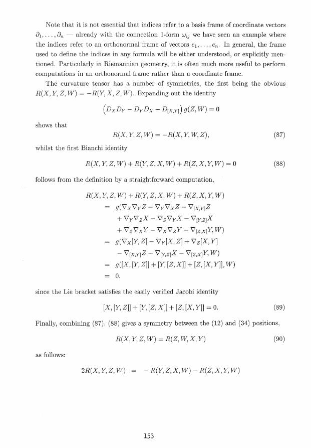
The curvature tensor has a number of symmetries, the first being the obvious

R(X, Y, Z, W) = -R(Y,X, Z, W). Expanding out the identity

(DxDy- DyDx- D[x,YJ) g(Z, W) = 0

shows that

R(X, Y, Z, W) = -R(X, Y, W, Z),

whilst the first Bianchi identity

R(X, Y, Z, W) + R(Y, Z, X, W) + R(Z, X, Y, W) = 0

follows from the definition by a straightforward computation,

R(X, Y, Z, W) + R(Y, Z, X, W) + R(Z, X, Y, W)

g("Vx'\lyZ- '\ly'\lxZ- "V[x,Y]Z

+ '\ly'\lzX- '\lz'\lyX- "V[Y,z]X

+ '\7 z '\7 x Y- '\7 x '\7 z Y- "V[z,x]Y, W)

g('\7 x[Y, Z]- '\ly[X, Z] + '\7 z[X, Y]

- "V[x,Y]Z- "V[Y,z]X- "V[z,x]Y, W)

g([X, [Y, Z]] + [Y, [Z, X]] + [Z, [X, Y]], W)

0,

since the Lie bracket satisfies the easily verified Jacobi identity

[X, [Y, Z]] + [Y, [Z, X]] + [Z, [X, Y]] = 0.

(87)

(88)

(89)

Finally, combining (87), (88) gives a symmetry between the (12) and (34) positions,

R(X, Y, Z, W) = R(Z, W, X, Y) (90)

as follows:

2R(X, Y, Z, W) - R(Y, Z, X, W) - R(Z, X, Y, W)

153

+ R(Y, W, X, Z) + R(W, X, Y, Z)

R(X, Y, Z, W) + R(X, Y, Z, W)

+ R(Y, Z, W, X)+ R(Z, X, W, Y)

- R(Z, W, Y, X)- R(W, Z, X, Y)

2R(Z, W, X, Y).

The definition of Riem can be written in terms of a commutator of covariant deriva­

tives R(X, Y, Z, W) = g(R(X, Y)Z, W), where

R(X, Y)Z = ('Vx'Vy- Vy'Vx- V[x,YJ)Z. (91)

In index notation and with a coordinate frame we have

where Rijk e = Rjkp9pf and (g;j) = (gi/) is the inverse metric. This process of raising

and lowering of indices using the metric and its inverse, corresponds to the canonical

isomorphisms between TpM and r; M defined by the inner product g. Using the ·;;

notation for covariant derivative yields the so-called Ricci identity

(92)

Applying the metric isomorphism to the differential df of a function f E C 00 (M)

gives the gradient operator,

(93)

where !;i = 8d. Another way of stating the definition of gradf is

g(gradf,X) = Dxf = df(X), for all vectors X. (94)

Taking the covariant derivative of gradf gives the Hessian, or second covariant deriva­

tive matrix of f, v7jf = !;ij = aiajJ- r:jakf, (95)

and the trace of \72 f is the Laplace-Beltrami operator of the metric g

(96)

154

where V§ = Vde[g. Another method for describing the curvature and covariant derivatives was de­

veloped by E. Cartan, and uses orthonormal frames and forms, rather than vectors.

Because forms behave better than vectors under maps of manifolds, the Cart an calculus

is frequently better suited to actual computations.

For this we need the exterior derivative operator

which is a linear first order differential operator satisfying

(a) d(f) = dj, for j E C 00 (M);

(b) d(a 1\ (3) = da 1\ (3 + ( -l)ka 1\ d/3, for a E Ak(M);

(c) d2 = 0.

(97)

These properties uniquely determine d, since they lead to an explicit expression for d

in any local coordinate system. Firstly, (a) determines d acting on A(M) = C 00 (M).

By (b) and (c), for any two functions j, g E coo ( M) we have

d(f dg) df 1\ dg + f d(dg)

df 1\ dg,

which determines don A 1(M) since alll-forms may be written as a linear combination

of terms of the form f dg. Now

and thus by induction it follows that

for any functions g1 , ... , 9k· Hence

(98)

which shows that the conditions (a), (b), (c) determine don Ak(M). To show that

this definition is consistent, we note that any k-form may be written as a = a dxi1 1\

... 1\ dxik = a 1 dx1 where the coefficients ai1 ···ik = a 1 are uniquely determined and

I= (i1 < · · · < ik) is a multi-index. Then the local definition

Oaf i I da = ~dx 1\ dx ,

ux'

155

(99)

satisfies the required properties, and (98) shows that any definition of dis unique (since

the differentials dg1 are defined already), hence there exists a unique operator with the

properties (a), (b), (c). By iterating (99) we see that the property d2 = 0 reflects the

commutativity of second partial derivatives.

By combining (71) and (98) we see that d behaves naturally under pullback by a

map 1> : M -+ N,

cf>*(da) = d(cf>*a), Va E A(N). (100)

By computing in local coordinates, we can easily show that for any a E A1 (M) and

vector fields X, Y E X(M),

da(X, Y) = Dx(a(Y))- Dy(a(X))- a([X,Y]). (101)

A standard exercise relates d acting on A(R3 ) to the classical differential operators

div, grad and curl.

Now suppose e1, ... , en is an orthonormal frame, and let ell ... , en be the dual

covector frame. From (101) we have

- e;([ej, ek])

- g(e;, 'Veiek- 'Vekei)

W;j(ek)- Wik(eJ)

- (wie 1\ ee) (ej, ek),

which gives Cartan's first structure equation

(102)

where w;1 = g(e;, \lei) is the connection 1-form. A similar computation yields the

second structure equation,

(103)

where rl;1 is the curvature 2-form and is related to the Riemann curvature tensor by

where the indices in R;1ke refer to components in the basis e1 , ... , en­

The first Bianchi identity (88) is equivalent to

156

(104)

(105)

and is derived (much more easily this time!) by taking the exterior derivative of (102).

Taking the exterior derivative of D;j using (103) gives the Cartan form of the second

Bianchi identity

(106)

which is equivalent to

(V'xR)(Y, Z)W + (\7yR)(Z,X)W + (V'zR)(X, Y)W = 0, (107)

a form which can be verified directly, but not so simply, from the definition of Riem

and \7 Riem. The index notation versions of (105) and (106) are

R[ijk]£ = 0, Rij[kf;m] = 0, (108)

where enclosing indices in square brackets indicates a total antisymmetrisation over

those indices, ie. [ijk] = i(ijk- ikj + jki- jik + kij- kji).

157

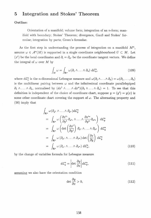
5 Integration and Stokes' Theorem

Outline:

Orientation of a manifold; volume form; integration of an n-form; man­

ifold with boundary; Stokes' Theorem; divergence, Gauf3 and Stokes' for­

mulae; integration by parts; Green's formulae.

As the first step in understanding the process of integration on a manifold Mn, assume w E An(M) is supported in a single coordinate neighbourhood U C M. Let

(xi) be the local coordinates and o; = Oxi be the coordinate tangent vectors. We define

the integral of w over M by

(109)

where d£~ is then-dimensional Lebesgue measure and w(o1 1\ ... 1\ On) = w(o1 , ••• , On)

is the multilinear pairing between w and the infinitesimal coordinate parallelepiped

o1 1\ ... 1\ On, normalised by ( dx 1 1\ ... 1\ dxn) ( o1 1\ ... 1\ On) = 1. To see that this

definition is independent of the choice of coordinate chart, suppose y = (yi) = y(x) is

some other coordinate chart covering the support of w. The alternating property and

(56) imply that

(110)

by the change of variables formula for Lebesgue measure

(111)

assuming we also have the orientation condition

oy det ox > 0, (112)

158

restricting the admissible coordinate charts.

We say that M is orientable ifthere is f.L E An(M) such that f.L # 0 everywhere in M;

an oriented coordinate chart then is required to satisfy f.L(81/\ .. . l\8n) > 0. Equivalently,

an orientable manifold is one with a covering by coordinate charts satisfying (112).

The problem of integrating a general w E An(M) is reduced to the case of support

within a coordinate neighbourhood by the use of a partition of unity: a family of

functions ,\"' E coo ( M), a E A, satisfying 0 :::; ,\"' (p) :::; 1 and La Aa (p) = 1 for all

p E M, where only a finite number of terms in the sum are non-zero. If M is separable,

then a partition of unity exists subordinate to any locally finite covering of M.

Writing w =La AaW and using the linearity of JM then determines fM w. Note that

this definition of JM w depends strongly on the choice of orientation f.L E An(M) of

M: denoting by -M the manifold with the reverse orientation -f.L, we have f(-M)w = -fMw.

If ¢ : Mm --+ Nn and if a E Am(N) then the integral of a over M is defined

naturally by pull-back:

r a= r ¢*(a). }q,(M) }M

(113)

This applies in particular to the situation where M is a submanifold of N and ¢ is the

inclusion map, which shows that there is a natural dual pairing between Ak(N) and

k-dimensional submanifolds of N, given by integration along the submanifold.

On an oriented Riemannian manifold we may normalise the orientation form to

satisfy II Mil = 1, where IIMII denotes the metric length. This normalised n-form is called

the volume form of M. In local (oriented) coordinates we have

(114)

where det(g) = det(9;;), g;j = g(8;,8j)· Under a change of coordinates y = y(x) we

have

and thus the volume form f.L defined by (114) is independent of the choice of oriented

coordinate system.

If M is Riemannian but not oriented then it is still possible to define an integral for

functions (but not n-forms), by using the measure Jdet(g) d£~ in coordinate patches.

159

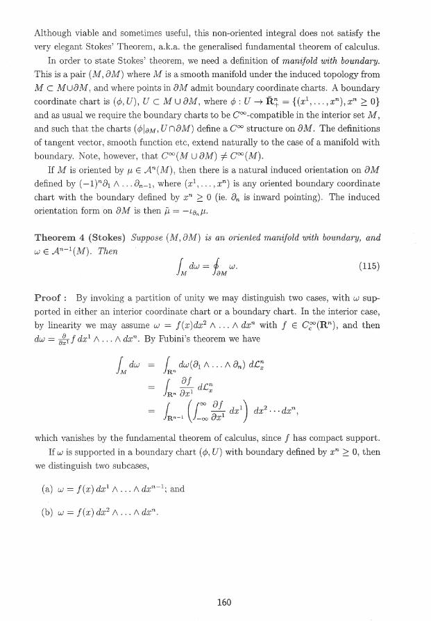
Although viable and sometimes useful, this non-oriented integral does not satisfy the

very elegant Stokes' Theorem, a.k.a. the generalised fundamental theorem of calculus.

In order to state Stokes' theorem, we need a definition of manifold with boundary.

This is a pair (M, oM) where M is a smooth manifold under the induced topology from

M c MUoM, and where points in oM admit boundary coordinate charts. A boundary

coordinate chart is (c/J, U), U c M u oM, where ¢J: U-+ R+ = {(x\ ... , xn), xn 2 0} and as usual we require the boundary charts to be C 00-compatible in the interior set M,

and such that the charts (c/JiaM, UnoM) define a coo structure on oM. The definitions

of tangent vector, smooth function etc, extend naturally to the case of a manifold with

boundary. Note, however, that C00 (M u oM) # C00 (M).

If Misoriented by 11 E An(M), then there is a natural induced orientation on oM defined by ( -1) n o1 1\ ... On_1 , where ( x1, ... , xn) is any oriented boundary coordinate

chart with the boundary defined by xn 2 0 (ie. On is inward pointing). The induced

orientation form on oM is then [1. = -Lan/1·

Theorem 4 (Stokes) Suppose (M, oM) is an oriented manifold with boundary, and

wE An-1(M). Then

r dw = 1 w. }M JaM

(115)

Proof : By invoking a partition of unity we may distinguish two cases, with w sup­

ported in either an interior coordinate chart or a boundary chart. In the interior case,

by linearity we may assume w = f(x)dx2 1\ ... 1\ dxn with f E C~(Rn), and then

dw = 8~1 f dx1 1\ ... 1\ dxn. By Fubini's theorem we have

which vanishes by the fundamental theorem of calculus, since f has compact support.

If w is supported in a boundary chart ( c/J, U) with boundary defined by xn 2 0, then

we distinguish two subcases,

(a) w = f(x) dx1 1\ ... 1\ dxn- 1; and

(b) w = f(x) dx2 1\ ... 1\ dxn.

160

In care (a} we have

and thus

Since-

dw. { "1..\_"--1 8.-J .J;; 1 d. ,.,_ = - :Jc.J -;;--ux A ... A X , uxn-

{ .. dw(llt A .•• Aa,...)d£: . '1-

- '-l}n-t- £. . (too uf dx'"t dx1 ... fixn-r iJl>'-1 Jo. &~ '

= (-lt-1 £ .. _Jf(lf,x")Jf'; dx1 • • -dxn-l

= {-tt £.,_1 ftx',Jl} d.C:;,-1-

on oM, we see that the final expression is just faM w as req_uired.

The final sub case (b) with w not involving dxn is computed similarly, but the interior

integral is now f.':"oo a':,d(x', 0) dx1 which again vanishes by the fundamental theorem

of calculus and the compact support of f. • If M is an oriented Riemannian manifold and J.L. is the metric volume form, then we

can define the divergence of a vector fietd X E X(M) by

divX J.L = d(txJ.L). (116)

In coordinates,

= X~. (117)

The divergence form of Stokes's theorem is thus

{ divXJ.L= 1 txJ.L, }M JaM

(118)

which we may write in a more familiar form by noting that the induced oriented volume

form on oM is defined by Jt = LnJ.L, where n E Tp(M u oM), p E oM, is the outward

pointing unit normal to aM. This implies that

txp = g(X, n }ij + a term involving dx",

so. that { divX J.L = ,£- g{X, n)it.

fM JaM (Uft)

161

This reduces to the well-known Gaul3 and Green's formulae in dimensions' 3 and .2

respectively.

A more general form of (119) is sometimes useful, for example when integrating

along a null hypersurface in a Lorentzian manifold, where the metric volume ·form

vanishes and it is not possible to define a unit length normal vectpr. If f.L and jl

are orientation forms on M and 8 M ,respectively, then there is a 1-form v such that

f.L = v 1\ P,; vis called a conormal to a}vf. Then (118) gives

( d(ix!L) = 1 v(X) P,. }M laM .

(120)

To derive the classical Stokes' theorem for the integral ofcurl V over a surface S

in R 3 we need to pull back from the surface to R2 with the parameterisatiori map

X : U C R 2 --+ S c R 3 . Details are left as an exercise.

Several useful identities may be obtained from the divergence form of Stokes' the­

orem. Choosing a vector field of the form f X, where f E c= ( M) and X E X ( M), we

find

( (fdivX + Dx(f)) dvM = 1 f g(X, n) dS, }M ~M

(121)

where we use the common notation dvM = M and dS = P, for the volume forms of M

and aM respectively.

Comparing (93), (96) and (117) we see that

D-gf = div(gradf); (122)

the divergence identity applied with X = gradf gives

(123)

where Dnf is the outer normal derivative of f. Combining (121) and (123) gives the

Green's identities for two functions ¢, 'ljJ E c=(M),

r 'l/JD.g¢dv }M

JM ('l/JD-9¢- cpD-9 '1/J) dv

- ( g(gradcp,grad'lj;)dv+ 1 '1/JDncpdS, (124) }M ~M

1 ( '1/JDnc/!- c/!Dn 'ljJ) dS. (125) laM

These identities enable us to integrate by parts over a manifold, and turn out to be

very useful in studying the functions and operators associated with M. For example,

we have

Corollary 5 Suppose M is a connected compact oriented manifold without boundary.

The only harmonic functions (ie. satis-fyi'M 6.9 cp = 0} on M are constants.

162

Proof: Applying (124) with¢= '1/J gives

( ¢!:::.9 ¢ dv + f g(grad¢, grad¢) dv = J ¢ Dn¢ dS. }M }M ~M

Since aM= 0 and !:::.9 ¢ = 0 this gives

JM g(grad¢, grad¢) dv = 0.

Since g is positive definite, it follows that grad¢ = 0 identically, hence ¢ is constant.

II

In a similar fashion we may prove uniqueness for solutions u E C2 (M) of the

Dirichlet problem

in M } on 8M

(126)

where f E C0 (M) and ¢ E C0 (8M) are given. For, suppose u 1, u2 are two solutions

of (126), then the difference w = u1 - u2 satisfies the Dirichlet problem with f = 0

and zero boundary conditions. The previous argument carries over and shows that w

is constant, hence w = 0 identically by the zero boundary conditions.

163