introduction to constructive logic and mathematics
TRANSCRIPT

Introduction toConstructive Logic and Mathematics
Thomas Streicher
WS 00/01

Prerequisites
The aim of this course is to give an introduction to constructive logic and math-ematics for people who have some basic acquaintance with naive set theory andthe formalism of first order logic (propositional connectives and quantifiers) asusually acquired within the first year when studying mathematics or computerscience. It were desirable to know the basic notions of computability theory (re-cursion theory) but for reasons of selfcontainedness we will give a crash course /recap of computability theory later on when we need it. Besides that one shouldhave seen once a construction of the real numbers though its constructive variantwill be introduced and studied in detail.
1

Contents
1 Introduction 3
2 Natural Deduction 7
3 A Hilbert Style System 14
4 Truth–Value Semantics of Constructive Logic 15
5 Embedding Classical into Constructive Logic 19
6 Constructive Arithmetic and Analysis 24
7 Constructive Real Numbers 30
8 Basic Recursion Theory in HA 36
9 Kleene’s Number Realizability 39
10 Markov’s Principle 48
11 Kleene’s Function Realizability 49
12 Higher Type Arithmetic 5212.1 Description of HAω . . . . . . . . . . . . . . . . . . . . . . . . . . 5412.2 Models of HAω . . . . . . . . . . . . . . . . . . . . . . . . . . . . 56
13 Kreisel’s Modified Realizability 58
14 Godel’s Functional Interpretation 65
2

1 Introduction
Constructive Logic and Mathematics has always existed as a trend in mainstreammathematics. However, the need of developing it as a special branch of math-ematics did not arise before beginning of the 20th century when mathematicsbecame more abstract and more inconstructive due to the influence of set the-ory. Inconstructive methods have dominated (the presentation) of 20th centurymainstream mathematics. However, during the last 30 years—mainly triggeredby the growing influence of computer science—we have experienced an increasinginterest in constructive mathematics typically for the following reason.If we have proved ∀n.∃m.A(n,m) then we want to read off from this proof analgorithmic function f for which we can show that ∀n.A(n, f(n)), i.e. we want toextract an algorithm from a proof of existence. Clearly, if A(n,m) is a decidableproperty of natural numbers then from the mere validity of ∀n.∃m.A(n,m) weobtain a most stupid algorithm computing an m with A(n,m) for every n: searchthrough the natural numbers until you find (the first) m with A(n,m). But veryoften one can read off a much more intelligent algorithm from a (constructive)proof of ∀n.∃m.A(n,m).However, if A is not decidable this is not possible anymore in the general caseeven if m does not depend on n. Consider for example the formula
∃x. (P (x) → ∀y. P (y))
of pure predicate logic where P is an unspecified predicate constant of arity 1.Classically this is a tautology as if ∀y.P (y) holds then x can be chosen arbitrarilyand if ¬∀y.P (y) then there exists an a with ¬P (a) which we may choose for x.However, what is sort of intriguing is that this proof does not provide us with aconcrete a for which we could show P (a) → ∀y. P (y). One easily sees that therecannot exist a term t for which P (t) → ∀y. P (y) is valid (in all models).One might think that this defect has to do with the general nature of the predicateP whose nature is left absolutely unspecified. But the following example showsthat we may run into a problem also for very concrete existence statements.
Theorem 1.1 There are irrational numbers a and b such that ab is rational.
Proof: Suppose that√
2√
2is rational then put a = b =
√2. Otherwise if
√2√
2is
irrational then we may put a =√
2√
2and b =
√2 which are both irrational but
ab = (√
2√
2)√
2 =√
2(√
2·√
2)=√
22
= 2
is certainly rational. 2
This proof—though undoubtedly correct w.r.t. the usual standards—does not tell
us how to choose a and b unless we have decided whether√
2√
2is rational. But
3

deciding whether√
2√
2is rational or not is a non–trivial problem whose answer
is not at all implicit in the proof just given.Another example exhibiting the “defects” of classical logic comes from theoreticalcomputer science. Consider the predicate
A(n,m) ≡ m = 0 ↔ {n}(n)↓
where {n} stands for the partial function computed by the nth Turing machineand e↓ stands for “e is is defined” (accordingly we write e↑ when e is undefined).Now using classical reasoning one easily proves ∀n.∃m.A(n,m) as if {n}(n)↓ thenput m = 0 and otherwise put m = 1, say. But, there cannot exist an algorithmicfunction f with
∀n.f(n) = 0 ↔ {n}(n)↓
as otherwise the halting problem were decided by f .1
The next example of a non–constructive existence proof is taken from basic clas-sical analysis where one of the first theorems is the following.
Theorem 1.2 For every bounded sequence (xn)n∈N of real numbers there existsa point of accumulation.
Proof: Let [a, b] be a rational interval containing all xn (which exists as by as-sumption the sequence (xn)n∈N is bounded). A point of accumulation is givenby the nesting of intervals [an, bn]n∈N which is “constructed” as follows: put[a0, b0] := [a, b] and
[an+1, bn+1] =
{[an,
an+bn
2] if ∀m.∃k ≥ m.xk ∈ [an,
an+bn
2]
[an+bn
2, bn] otherwise .
2
Notice that the “construction” of [an+1, bn+1] from [an, bn] cannot be performedalgorithmically as one has to decide whether the interval [an,
an+bn
2] contains
infinitely many items of the sequence (xn)n∈N which surely cannot be achieved infinite time.
1It is a basic fact from recursion theory that K = {n ∈ N | {n}(n)↓} is not decidable.Otherwise there would exist a Godelnumber e such that
{e}(n)↓ iff {n}(n)↑
leading to the contradiction{e}(e)↓ iff {e}(e)↑
when instantiating n by e (a trick called diagonalisation). Obviously, from the undecidabilityof K there follows immediately the undecidability of the halting set H = {〈n, m〉 | {n}(m)↓}.
Notice that diagonalisation arguments are all instances of the (constructive) tautology¬∃x.∀y. R(x, y) ↔ ¬R(y, y).
4

Thus, apparently the use of classical reasoning allows one to prove existentialstatements whose witnessing object cannot be read off from the argument. Crit-ical examination of the above examples tells us that this lack of constructivityoriginates from the use of the (classically correct) principles
(1) ∀y.P (y) ∨ ¬∀y.P (y)
(2) ¬∀y.P (y) ↔ ∃y.¬P (y)
(3)√
2√
2is either rational or irrational
(4) {n}(n)↓ ∨ {n}(n)↑
(5) (∀m.∃k ≥ m.xk ∈ [an,an+bn
2]) ∨ ¬(∀m.∃k ≥ m.xk ∈ [an,
an+bn
2]).
Propositions (1), (3), (4) and (5) are instances of the schema
PEM A ∨ ¬A
called Principle of Excluded Middle characteristic for classical logic. Use of PEMmay render proofs inconstructive as in general we cannot decide for a propositionA whether A or ¬A holds. This is typically the case if A is of the form ∀x.B(x) asone would have to examine infinitely many B(n) if x ranges e.g. over the naturalnumbers.As long as one is not interested in extracting algorithms from existence proofsthere is nothing to complain about classical logic. Most steps even in a classicalproof are constructive but sometimes there is made appeal to an oracle decidingthe truth of a proposition.In a sense it is true that constructive logic is obtained from classical logic byomitting PEM. But the question is what are the constructively valid principlesof reasoning. This is not so easy to answer as there are logical principles whichat first sight look different from PEM but whose proof requires PEM or is evenequivalent to it. For example the logical principle (2) above is usually provedvia PEM making a case analysis on ∃y.¬P (y): if ∃y.¬P (y) then ¬∀y.P (y) andif ¬∃y.¬P (y) then ∀y.¬¬P (y) from which it follows that ¬∀y.¬P (y). Anotherlogical principle familiar from classical reasoning is reductio ad absurdum
RAA ¬¬A→ A
where in order to prove A one refutes ¬A. We shall see later that the principlesPEM and RAA are equivalent and adding either of them to constructive logicone obtains classical logic.Having seen that it is not so obvious to identify what are “constructively valid”principles of reasoning we will discuss this question next. Usually, classical valid-ity is explained in terms of truth values, i.e. one explains what is the truth valueof a compound formula in terms of the truth values of its constituent formulas.
5

This will not work for constructive validity as ordinary truth value semanticsdoes validate PEM. Accordingly, the constructive meaning of propositions is ex-plained best in terms of an alternative semantics based on an (informal) notionof “proof” instead of an (informal) notion of “truth value”. Here “proof” shouldnot be understood in the sense of a formal proof in some logical calculus as givenfor example by a derivation tree but rather as an informal basic notion (like truthin case of classical logic). One can say that the meaning of constructive logicis best understood in terms of a proof semantics as opposed to the well-knowntruth–value semantics appropriate for classical logic. What we have called “proofsemantics” is often called Brouwer–Heyting–Kolmogoroff Interpretation (or sim-ply BHK Interpretation) after the people who brought it up.
Proof Semantics of Constructive Logic
ConjunctionA proof of A ∧B is a pair 〈p, q〉 where p is a proof of A and q is a proof ofB.
ImplicationA proof of A → B is a (constructive) function f mapping proofs of A toproofs of B, i.e. f(p) is a proof of B whenever p is a proof of A.
FalsityThere is no proof of ⊥ (falsity).
DisjunctionA proof of A∨B is either a proof of A or a proof of B where it is indicated(e.g. by a label) whether it proves A or B.
Universal QuantificationA proof of ∀x.A(x) is a (constructive) function f such that f(d) is a proofof A(d) for all d ∈ D where D is the domain of discourse (over which thevariable x ranges).
Existential QuantificationA proof of ∃x.A(x) is a pair 〈d, p〉 where d ∈ D and p is a proof of A(d)where D is the domain of discourse (over which the variable x ranges).
The clauses for implication and universal quantification may appear as “circular”and actually are. However, this is the case as well for the traditional 2–valuedtruth value semantics of classical logic where the logic to be explained is used onthe meta–level.2 Accordingly, the BHK interpretation must not be understood as
2If in classical logic one defines A→B as ¬A∨B then implication gets reduced to somethingmore primitive (in terms of the unexplained notions of negation and disjunction). However, this
6

a precise mathematical definition but rather as an informal, but intuitive explana-tion of meaning just as the ordinary truth semantics for classical logic. However,as we shall see later on there are variations of the BHK interpretation which havea precise technical meaning and are most useful in the sense that they provideinteresting models of constructive logic and allow us to give transparent proofsof metamathematical properties.
2 Natural Deduction
In this section we introduce a derivation calculus for constructive predicate calcu-lus which as close as possible reflects the structure of actual mathematical proofsand, therefore, has been baptized calculus of “Natural Deduction”3. Of course,derivations in this calculus are much more detailed than actual mathematicalarguments. It is not intended to develop constructive mathematics in a purelyformal way within such a calculus but rather to use it as a mathematical model ofactual constructive reasoning for which one may prove certain metamathematicalproperties exhibiting the nature of actual constructive reasoning.4
Notice that the syntax of predicate logic employed here deviates from the usualpractice in one particular aspect: instead of having negation as a basic proposi-tional connective we introduce a propositional constant ⊥ (‘falsity’) for the falseproposition and introduce negation via the ‘macro’ ¬A ≡ A→ ⊥. It is clear thatunder the usual 2–valued truth semantics we have that A → ⊥ is true iff A isfalse and, therefore, this ‘implementation’ of negation is in accordance the usualunderstanding of negation in classical logic.We suggest it as an informative exercise to explain the validity of the proof rulesof the following definition in terms of the BHK interpretation.
Definition 2.1 Sequents are expressions of the form
A1, . . . , An ` B
“explanation” of implication was always considered as somewhat contrived and not (properly)reflecting the intuitive understanding of implication which seems to be brought to the point bythe above clause for implication though in a somewhat “circular” way. On the other hand theBHK interpretation provides a proper reduction of disjunction and existential quantificationwhich are the two connectives where constructive logic really deviates from classical logic.
3Natural Deduction was introduced by G. Gentzen back in the 30ies as a mathematicalmodel of mathematical proofs. His aim was to prove—as strongly advocated by D. Hilbert—the consistency of arithmetic, i.e. that there is no derivation of a false proposition. Generally,the endeavour of analyzing proofs by mathematical methods is called proof theory. Nowadays,however, consistency proofs are not the holy grail of proof theory anymore as their foundationalvalue is more than debatable due to Godel’s (Second) Incompletness Theorem.
4Of course, the same applies to formalisations of classical logic. However, as classical rea-soning is more familiar to most mathematicians than constructive reasoning for studying thelatter it is worthwhile to explicitly state the proof rules from the very beginning.
7

where the Ai and B are formulas of predicate logic. The intended meaning is thatthe assumptions A1, . . . , An entail conclusion B. The valid sequents of CPL(Constructive Predicate Logic) are defined inductively via the following proofrules.
Structural Rules
(ax)Γ, A,∆ ` A
Γ, A,B,∆ ` C(ex)
Γ, B,A,∆ ` C
Γ ` C(w)
Γ, A ` C
Γ, A,A ` C(c)
Γ, A ` C
Propositional Connectives
Γ ` A Γ ` B(∧I)
Γ ` A ∧B
Γ ` A1 ∧ A2(∧Ei)
Γ ` Ai
Γ, A ` B(→ I)
Γ ` A→ B
Γ ` A→ B Γ ` A(→ E)
Γ ` B
Γ ` Ai(∨Ii)
Γ ` A1 ∨ A2
Γ ` A ∨B Γ, A ` C Γ, B ` C(∨E)
Γ ` C
Γ ` ⊥(⊥E)
Γ ` C
Quantifiers
Γ ` A(x) x 6∈ FV (Γ)(∀I)
Γ ` ∀x.A(x)
Γ ` ∀x.A(x)(∀E)
Γ ` A(t)
Γ ` A(t)(∃I)
Γ ` ∃x.A(x)
Γ ` ∃x.A(x) Γ, A(x) ` C x 6∈ FV (Γ, C)(∃E)
Γ ` C
♦
Notice that there are two elimination rules (∧E1) and (∧E2) for conjunction andtwo introduction rules (∨I1) and (∨I2) for disjunction.
8

It is absolutely necessary to take the variable conditions serious in rules (∀I) and(∃E) as the following counterexamples show where faulty applications of theserules are marked by †.That in rule (∀I) the variable x must not occur in the premiss is demonstratedby the following pseudo–derivation
(ax)A(x) ` A(x)
(∀I)†A(x) ` ∀x.A(x)
(→ I)` A(x) → ∀x.A(x)
(∀I)` ∀x.(A(x) → ∀x.A(x))
(∀E)` A(t) → ∀x.A(x)
That in rule (∃E) the variable x must not occur freely in C is demonstrated bythe following pseudo–derivation
(ax)∃x.A(x) ` ∃x.A(x)
(ax)∃x.A(x), A(x) ` A(x)
(∃E)†∃x.A(x) ` A(x)
(∀I)∃x.A(x) ` ∀x.A(x)
That in rule (∃E) the variable x must not occur freely in Γ is shown by thefollowing pseudo–derivation
(ax)Γ ` ∃x.¬A(x)
(ax)Γ,¬A(x) ` ¬A(x)
(ax)Γ,¬A(x) ` A(x)
(→ E)Γ,¬A(x) ` ⊥
(∃E)†A(x),∃x.¬A(x) ` ⊥
(→ I)∃x.¬A(x) ` ¬A(x)
(∀I)∃x.¬A(x) ` ∀x.¬A(x)
where Γ ≡ A(x),∃x.¬A(x).The consideration of these pseudo–derivations should have already conveyed somefeeling for how to construct formal derivations in the calculus of Natural Deduc-tion. But, of course, in correct derivations in all applications of the rules (∀I)and (∃E) the variable conditions have to be fulfilled. We now consider quite afew examples of correct derivations in CPL as well as derived rules not just forgetting familiar with the practice of the construction of formal proofs but also tohave these constructive logical principles available for subsequent use.
9

The derivation(ax)
A,¬A ` ¬A(ax)
A,¬A ` A(→ E)
A,¬A ` ⊥(→ I)
A ` ¬¬A
demonstrates that a proposition entails its double negation.However, a negated formula ¬A follows from its double negation ¬¬¬A via thederivation
(ax)¬¬¬A,A ` ¬¬¬A
(ax)A,¬A ` ¬A
(ax)A,¬A ` A
(→ E)A,¬A ` ⊥
(w)¬¬¬A,A,¬A ` ⊥
(→ I)¬¬¬A,A ` ¬¬A
(→ E)¬¬¬A,A ` ⊥
(→ I)¬¬¬A ` ¬A
and, therefore, we easily can derive
¬A↔ ¬¬¬A
from which it follows that double negation is idempotent, i.e. that
¬¬A↔ ¬¬¬¬A
is derivable.5 This observation allows us to reduce multiple negations either tosimple negation or double negation. Classically, we also have ¬¬A → A (andtherefore also ¬¬A ↔ A) which logical principle is called reductio ad absurdumand distinguishes classical logic from constructive logic as we shall see later.Next we show that
A ∨B → C a` (A→ C) ∧ (B → C)
abbreviating
A ∨B → C ` (A→ C) ∧ (B → C) and (A→ C) ∧ (B → C) ` A ∨B → C
as suggested by the notation.
5The phrase “A is derivable” is an abbreviation for “`A is derivable”. Moreover, notice thatA ↔ B is a ‘macro’ for (A → B) ∧ (B → A).
10

We have
(ax)A ∨B → C,A ` A ∨B → C
(ax)A ∨B → C,A ` A
(∨I1)A ∨B → C,A ` A ∨B
(→ E)A ∨B → C,A ` C
(→ I)A ∨B → C ` A→ C
and similarly one proves A ∨ B → C ` B → C form which it follows thatA ∨B → C ` (A→ C) ∧ (B → C).Now we derive the reverse direction. We have
(ax)Γ ` A ∨B Γ, A ` C Γ, B ` C
(∨E)(A→ C) ∧ (B → C), A ∨B ` C
(→ I)(A→ C) ∧ (B → C) ` A ∨B → C
where Γ stands for the context (A→C) ∧ (B→C), A ∨ B. The open assumptionΓ, A ` C can be derived as follows
(ax)Γ, A ` (A→ C) ∧ (A→ C)
(∧E1)Γ, A ` A→ C
(ax)Γ, A ` A
(→ E)Γ, A ` C
and similarly for the other open assumption Γ, B ` C.Notice that from ((A → C) ∧ (B → C)) ↔ (A ∨ B → C) there immediatelyfollows the ‘deMorgan’ law
¬A ∧ ¬B ↔ ¬(A ∨B)
instantiating C by ⊥. Further instantiating B by ¬A we get
¬(A ∨ ¬A) ↔ (¬A ∧ ¬¬A)
and as one easily derives¬(¬A ∧ ¬¬A)
it follows (Exercise!) that¬¬(A ∨ ¬A)
11

holds constructively. Thus, by reductio ad absurdum6 we get PEM. On the otherhand PEM entails reductio ad absurdum as can be seen from the derivation
(ax)Γ ` A ∨ ¬A
(ax)Γ, A ` A
(ax)Γ,¬A ` ¬¬A
(ax)Γ,¬A ` ¬A
(→ E)Γ,¬A ` A
(∨E)A ∨ ¬A,¬¬A ` A
(→ I)A ∨ ¬A ` ¬¬A→ A
where Γ ≡ A ∨ ¬A,¬¬A.Next we show that
∃x.A(x) → B a` ∀x.(A(x) → B)
provided x is not free in B. The direction from left to right is given by thederivation
(ax)∃x.A(x) → B,A(x) ` ∃x.A(x) → B
(ax)∃x.A(x) → B,A(x) ` A(x)
(∃I)∃x.A(x) → B,A(x) ` ∃x.A(x)
(→ E)∃x.A(x) → B,A(x) ` B
(→ I)∃x.A(x) → B ` A(x) → B
(∀I)∃x.A(x) → B ` ∀x.(A(x) → B)
and the reverse direction is given by the derivation
(ax)Γ ` ∃x.A(x)
(ax)Γ, A(x) ` ∀x.(A(x) → B)
(∀E)Γ, A(x) ` A(x) → B
(ax)Γ, A(x) ` A(x)
(→ E)Γ, A(x) ` B
(∃E)∀x.(A(x) → B),∃x.A(x) ` B
(→ I)∀x.(A(x) → B) ` ∃x.A(x) → B
where Γ ≡ ∀x.(A(x) → B),∃x.A(x). Instantiating B by ⊥ we get the ‘deMorgan’law
¬∃x.A(x) ↔ ∀x.¬A(x) .
Notice, however, that as we shall see later the dual deMorgan law
¬∀x.A(x) ↔ ∃x.¬A(x)
6But notice that the schema ¬¬A → A has to be instantiated by A ∨ ¬A ! Actually, as wewill see later on for a particular proposition it may hold that ¬¬A → A but not A ∨ ¬A.
12

is not constructively valid.We conclude this section by exhibiting some derived rules.First of all we have the most useful cut rule
Γ ` A Γ, A ` B(cut)
Γ ` B
which allows us to remove unnecessary assumptions from a sequent. Its correct-ness is immediate from the derivation
Γ, A ` B(→ I)
Γ ` A→ B Γ ` A(→ E)
Γ ` B
with open assumptions Γ ` A and Γ, A ` B.By definition for every connective of CPC there is a rule for its introduction onthe right of the turnstile. The following derived rules allow one to introdcuecompound formulas on the left of the turnstile
Γ, A,B ` C(∧L)
Γ, A ∧B ` C
Γ, A ` C Γ, B ` C(∨L)
Γ, A ∨B ` C
Γ ` A Γ, B ` C(→ L)
Γ, A→ B ` C(⊥L)
Γ,⊥ ` C
Γ, A(t) ` C(∀L)
Γ,∀x.A(x) ` C
Γ, A(x) ` C x 6∈ FV (Γ, C)(∃L)
Γ,∃x.A(x) ` C
We leave the verification of their correctness to the diligent reader.Notice that rule (∧L) can be inverted, i.e. we have
Γ, A,B ` C iff Γ, A ∧B ` C
and, therefore,
A1, . . . , An ` C iff A1 ∧ . . . ∧ An ` C
allowing us to reduce sequents to entailment between formulas.
13

We leave it as an exercise to show that the equivalences
C ` A ∧B iff C ` A and C ` B
A ∨B ` C iff A ` C and B ` C
C ` A→ B iff C ∧ A ` B
C ` ∀x.A(x) iff C ` A(x)
∃x.A(x) ` C iff A(x) ` C
where in the last two clauses x 6∈ FV (C) together with the rules
A ` A ⊥ ` AA ` B B ` C
A ` C
A ` B
A[t/x] ` B[t/x]
provide an alternative axiomatization of CPC. This axiomatization of entailmentbetween formulas will turn out as most useful when considering semantics.
3 A Hilbert Style System
Though the calculus of Natural Deduction most closely reflects the structure ofactual mathematical proofs (when spelt out in detail) for metamathematical pur-poses it is often convenient to use a Hilbert style system which inductively definesthe set of all formulas A such that ` A can be derived by Natural Deduction.The rules of such an inductive definition are of the form
A1, . . . , An ⇒ B
which means that B is provable provided A1, . . . , An are all provable. If n = 0then we simply write A instead of ⇒ A.
Theorem 3.1 The set of all formulas A of predicate logic for which the sequent` A is derivable in the calculus of Natural Deduction is defined inductively by thefollowing rules
(L1) A→ A
(L2) A , A→ B ⇒ B
(L3) A→ B , B → C ⇒ A→ C
(L4) A ∧B → A , A ∧B → B
(L5) C → A , C → B ⇒ C → A ∧B
14

(L6) A→ A ∨B , B → A ∨B(L7) A→ C , B → C ⇒ A ∨B → C
(L8) A ∧B → C ⇒ A→ B → C
(L9) A→ B → C ⇒ A ∧B → C
(L10) ⊥ → A
(L11) B → A(x) ⇒ B → ∀x.A(x) (x 6∈ FV (B))
(L12) ∀x.A→ A(t)
(L13) A(t) → ∃x.A(L14) A(x) → B ⇒ ∃x.A(x) → B (x 6∈ FV (B)).
Proof: One easily shows that if A can be derived via the rules (L1)–(L12) then` A can be proved by Natural Deduction.For the reverse direction one shows that if A1, . . . , An ` B can be derived in thecalculus of natural deduction then the formula A1 → . . .→ An → B is derivablevia the rules (L1)–(L14). 2
4 Truth–Value Semantics of Constructive Logic
Although proof semantics is conceptually more adequate as an explanation ofthe constructive meaning of propositional connectives and quantifiers we willintroduce in this section a truth–value semantics as an alternative. We willmainly use it for obtaining independence results, i.e. for showing that classicaltautologies (as e.g. A ∨ ¬A or ¬¬A → A) cannot be proved constructively. Itwill turn out that semantic proofs of underivability will be fairly simple due totheir ‘algebraic’ nature whereas direct purely syntactical proofs would be verycumbersome as they require a careful analysis of derivations as mathematicalobjects.The idea of truth–value semantics is to assign every formula a truth value, i.e. anelement of some structured set P of propositions.7 The distinguishing structureon propositions is given by a partial order ≤ thought of as entailment. In thelight of the discussion at the end of Section 2 conjunction/disjunction will beinterpreted as (binary) supremum/infimum and falsity will be interpreted as theleast element of the partial order (P,≤). Implication will turn out as anotherbinary operation which, however, is also fully determined by ≤. Such a kind ofposet (= partially ordered set) is axiomatized as follows.
7We have the tendency to understand the word ‘proposition’ in a semantical sense. A formulaor a sentences denotes a proposition. But we will not be consequent in this respect.
15

Definition 4.1 A Heyting algebra or Heyting lattice is a poset (A,≤) with finiteinfima and suprema such that for all a, b ∈ A there exists a→b ∈ A with
c ≤ a→b iff c ∧ a ≤ b
for all c ∈ A. Observe that a→b is uniquely determined by this property and,therefore, gives rise to a binary operation → on A called Heyting implication.
Notice that (in accordance with the subsequent definition of interpretation) wewrite ∧ for binary infimum and ∨ for binary supremum. Further notice that theexistence of a greatest element > in A is already ensured by → as c ≤ ⊥ → ⊥holds for all c ∈ A (where ⊥ stands for the least element of A).Heyting algebras provide enough structure to interpret the propositional part ofconstructive logic.
Definition 4.2 Let A be a Heyting algebra. A mapping ρ from PC, the set ofpropositional constants, to A is called a valuation (of propositional constants inA). Such a valuation ρ induces an interpretation of formulas of propositionallogic as given by the following inductive clauses
[[p]]ρ = ρ(p)[[A ∧B]]ρ = [[A]]ρ ∧A [[B]]ρ[[A ∨B]]ρ = [[A]]ρ ∨A [[B]]ρ[[A→ B]]ρ = [[A]]ρ→A [[B]]ρ[[⊥]]ρ = ⊥A
where ∧A, ∨A, →A and ⊥A stand for binary infimum, binary supremum, Heytingimplication and least element in A.
The proof of the following theorem is straightforward and recommended as aninstructive exercise as it reveals the ‘design decisions’ behind the definition ofHeyting algebra.
Theorem 4.1 If there is a derivation of the sequent A1, . . . , An ` B in (thepropositional part of) the calculus of Natural Deduction then
[[A1]]ρ ∧A . . . ∧A [[A1]]ρ ≤A [[B]]ρ
for every Heyting algebra A and valuation ρ in A.
This correctness theorem w.r.t. interpretation in Heyting algebras allows us toshow by purely semantical means that a sequent A1, . . . , An ` B is not derivable,namely by exhibiting appropriate A and ρ such that
[[A1]]ρ ∧A . . . ∧A [[A1]]ρ 6≤A [[B]]ρ .
Next we discuss a wide class of Heyting algebras among which we will find thecounterexamples needed for our independence results.
16

Example 4.1 Let X be a topological space. We write O(X) for the poset of opensubsets of X under subset inclusion. Then O(X) is a complete Heyting algebra.The poset has arbitrary joins given by set–theoretic union. Therefore, O(X) hasalso arbitrary infima (given by the interior of intersections). Thus, O(X) isa complete lattice, i.e. a poset with arbitrary infima and suprema. Notice thatfinite infima are given by ordinary set–theoretic intersections as open sets are bydefinition required to be closed under finite intersections. Accordingly, in O(X)there holds the following infinitary distributive law
U ∧∨i∈I
Vi =∨i∈I
U ∧ Vi
asU ∩
⋃i∈I
Vi =⋃i∈I
U ∩ Vi
holds for sets and joins and finite meets in O(X) are given by unions and fi-nite intersections, respectively. Due to this infinitary distributive law Heytingimplication in O(X) exists and is given by
U → V =⋃{W | U ∩W ⊆ V }
as it immediately follows from the infinite distributive law that (U → V )∩U ⊆ Vand U ∩W ⊆ V implies W ⊆ U → V .
The following particular instances will be most useful for providing counterex-amples.
Example 4.2 Let P be a poset and
dcl(P ) := {A ∈ P(P ) | y ≤ x ∈ A⇒ y ∈ A}
be the set of downward closed subsets of P partially ordered by ⊆. As P(P ) isclosed under arbitary unions and arbitrary intersections it certainly is a completeHeyting algebra (coming from a topological space). In this particular case Heytingimplication is given by
U→V = {p ∈ P | ∀q ≤ p. q ∈ U ⇒ q ∈ V }
where ↓p = {q ∈ P | q ≤ p}. This readily follows from the fact that U→V =⋃{↓p ∈ P | U ∩ ↓p ⊆ V } (Exercise!).
Having these classes of Heyting algebras at hand we can easily show that PEMand reductio ad absurdum are not derivable.
Theorem 4.2 In the calculus of Natural Deduction one cannot derive
¬¬p→ p p ∨ ¬p ¬p ∨ ¬q ↔ ¬(p ∧ q)
for propositional constants p and q.
17

Proof: Let A be the Heyting algebra dcl(2) where 2 is the poset 0 < 1 (i.e. theordinal 2). Let u = ↓0 for which we have
¬u = ⊥ and ¬¬u = >
and, therefore,
¬¬u = > > u and u ∨ ¬u = u ∨ ⊥ = u < > .
Thus, PEM and reductio ad absurdum cannot be derived.For refuting ¬p ∨ ¬q ↔ ¬(p ∧ q) consider the poset a < 1 > b with a and bincomparable. Let p = ↓a and q = ↓b. Then we have ¬p = q and ¬q = p and,therefore,
¬p ∨ ¬q = ↓{a, b} 6= {a, b, 1} = ¬∅ = ¬(p ∧ q) .
2
For complete Heyting algebras one may extend the interpretation of constructivepropositional logic to predicate logic in the following way. One chooses a set Das universe of discourse and n-ary predicates are interpreted as functions fromDn to A. Universal and existential quantification are interpreted as (possibly)infinite joins and meets in A which exist as A is assumed to be complete. Moreprecisely, we have
[[∃x.A(x)]]e =∨
d∈D[[A]]e[d/x][[∀x.A(x)]]e =
∧d∈D[[A]]e[d/x]
where e is an environment sending (object) variables to elements of A. Thisinterpretation of constructive predicate logic is quite in accordance with the usualTarskian semantics of classical predicate logic. The difference just is that the 2element Heyting algebra is replaced by arbitrary complete Heyting algebras.Though Heyting–valued models of CPC are an interesting topic8 we refrain frominvestigating them in greater detail.
Intermezzo on Kripke Semantics
It might be illuminating to give a more concrete version of the interpretationof propositional logic in cHa’s of the form dcl(P ) commonly known as Kripkesemantics. The key idea of Kripke semantics is to think of the poset P as a setof ‘possible worlds’ and of v ≤ u as “v is a possible development of u”. Themeaning of a proposition then is considered as a set of possible worlds “closedunder all possible developments”, i.e. as a downward closed subset of P .
8The adequate setting for Heyting–valued semantics is the theory of sheaves over a topolog-ical space or a cHa (complete Heyting algebra). Categories of sheaves are the basic examplesof so–called toposes which constitute a further even more general notion of model for higherorder constructive logic.
18
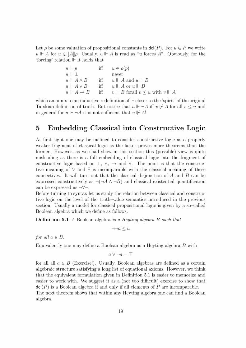
Let ρ be some valuation of propositional constants in dcl(P ). For u ∈ P we writeu A for u ∈ [[A]]ρ. Usually, u A is read as “u forces A”. Obviously, for the‘forcing’ relation it holds that
u p iff u ∈ ρ(p)u ⊥ neveru A ∧B iff u A and u Bu A ∨B iff u A or u Bu A→ B iff v B forall v ≤ u with v A
which amounts to an inductive redefinition of closer to the ‘spirit’ of the originalTarskian definition of truth. But notice that u ¬A iff v 6 A for all v ≤ u andin general for u ¬A it is not sufficient that u 6 A!
5 Embedding Classical into Constructive Logic
At first sight one may be inclined to consider constructive logic as a properlyweaker fragment of classical logic as the latter proves more theorems than theformer. However, as we shall show in this section this (possible) view is quitemisleading as there is a full embedding of classical logic into the fragment ofconstructive logic based on ⊥, ∧, → and ∀. The point is that the construc-tive meaning of ∨ and ∃ is incomparable with the classical meaning of theseconnectives. It will turn out that the classical disjunction of A and B can beexpressed constructively as ¬(¬A ∧ ¬B) and classical existential quantificationcan be expressed as ¬∀¬.Before turning to syntax let us study the relation between classical and construc-tive logic on the level of the truth–value semantics introduced in the previoussection. Usually a model for classical propositional logic is given by a so–calledBoolean algebra which we define as follows.
Definition 5.1 A Boolean algebra is a Heyting algebra B such that
¬¬a ≤ a
for all a ∈ B.
Equivalently one may define a Boolean algebra as a Heyting algebra B with
a ∨ ¬a = >
for all all a ∈ B (Exercise!). Usually, Boolean algebras are defined as a certainalgebraic structure satisfying a long list of equational axioms. However, we thinkthat the equivalent formulation given in Definition 5.1 is easier to memorize andeasier to work with. We suggest it as a (not too difficult) exercise to show thatdcl(P ) is a Boolean algebra if and only if all elements of P are incomparable.The next theorem shows that within any Heyting algebra one can find a Booleanalgebra.
19

Theorem 5.1 Let A be a Heyting algebra and
B := A¬¬ := {¬a | a ∈ A}
be the set of ¬¬–closed elements of A. This terminology makes sense as a ∈ Biff ¬¬a ≤ a. The set B of ¬¬–closed elements of A satisfies the following closureproperties
(1) ⊥,> ∈ B
(2) B is closed under ∧
(3) a→ b ∈ B whenever b ∈ B (for arbitrary a ∈ A).
Moreover, B considered as a sub–poset of A is a Boolean algebra where b1∨B b2 =¬(¬b1 ∧ ¬b2).
Proof: Let a ∈ A. Then we have a ≤ ¬¬a as a ∧ ¬a ≤ ⊥ and, therefore,¬¬¬a ≤ ¬a as ¬¬¬a∧ a ≤ ¬¬¬a∧¬¬a ≤ ⊥. Thus, it follows that A¬¬ consistsprecisely of negations of elements of A.As ⊥ = > → ⊥ and > = ⊥ → ⊥ it follows that > and ⊥ are in A¬¬.Suppose a, b ∈ A¬¬, i.e. ¬¬a = a and ¬¬b = b. Then a ∧ b = ¬¬a ∧ ¬¬b =¬(¬a ∨ ¬b) ∈ A¬¬ = B.Let a ∈ A and b ∈ B. Then ¬¬b = b and, therefore, a → b = a → ¬¬b =¬(a ∧ ¬b) ∈ A¬¬ = B.It remains to check that joins in B are given by b1∨B b2 = ¬(¬b1∧¬b2). Supposethat b1, b2 ∈ B, i.e. b1 = ¬¬b1 and ¬¬b2 = b2. Clearly, ¬(¬b1 ∧ ¬b2) ∈ A¬¬as its is negated. For i = 1, 2 we have that ¬b1 ∧ ¬b2 ≤ ¬bi and, therefore,bi = ¬¬bi ≤ ¬(¬b1 ∧ ¬b2) = b1 ∨B b2, i.e. b1 ∨ b2 is an upper bound of b1 andb2. We now show that it is the least upper bound in B. Suppose b1, b2 ≤ c ∈ B.Then ¬c ≤ ¬bi for i = 1, 2 and, accordingly, ¬c ≤ ¬b1∧¬b2 from which it followsthat b1 ∨B b2 = ¬(¬b1 ∧ ¬b2) ≤ ¬¬c = c as desired. 2
It is easy to see (by inspection of the proof we just gave) that for a cHa A thesubposet B = A¬¬ of double negation closed elements is a cBa. Infinite meets inB are inherited from A and
∨Bi∈I bi = ¬
∧i∈I ¬bi. Notice that for a topological
space X the Boolean algebra O(X)¬¬ is the subposet of O(X) on the so–calledregular open sets, i.e. those open sets U which coincide with the interior of theclosure of U (int(cl(U)) = U).After these simple algebraic considerations we apply a construction analogous to(−)¬¬ to the syntax of predicate logic.
20

Definition 5.2 The Godel–Gentzen double negation translation (−)G of formu-las of predicate logic is defined inductively as follows
⊥G ≡ ⊥PG ≡ ¬¬P P atomic but different from ⊥(A ∧B)G ≡ AG ∧BG
(A→B)G ≡ AG → BG
(A ∨B)G ≡ ¬(¬AG ∧ ¬BG)
(∀x.A)G ≡ ∀x.AG
(∃x.A)G ≡ ¬∀x.¬AG .
The double negation translation can be described informally as follows: atomicformulas are negated twice, ∧, →, ⊥ and ∀ are left unchanged but ∨ and ∃ arereplaced by their “de Morgan dual”. Obviously, the double negation translationis a syntactic analogue of Theorem 5.1 in the sense that classical connectives andquantifiers look as they have to be in A¬¬. Often (e.g. in constructive arithmetic)the basic predicates are decidable, i.e. satisfy PEM, and, therefore, one may definePG ≡ P for atomic formulas. However, in the general case atomic formulasdifferent9 from ⊥ have to be doubly negated. We leave it as an exercise toshow that the equivalence of AG and (AG)G can be proved constructively for allformulas A. Notice also that in general ¬¬A and AG are not provably equivalentin constructive logic (exercise!).The key result of this section will be the following
Theorem 5.2 A sequent A1, . . . , An ` B can be derived in classical predicatelogic if and only if its G–translation AG
1 , . . . , AGn ` BG can be derived in con-
structive predicate logic.
Notice, however, that in general A and AG are not provably equivalent in con-structive logic (e.g. if A is an appropriate instance of PEM) though they areprovably equivalent in classical logic.But before proving Theorem 5.2 we need the following notion.
Definition 5.3 The class of Harrop formulas is defined inductively by the fol-lowing clauses
• ⊥ is a Harrop formula
• A ∧B is a Harrop formula whenever A and B are Harrop formulas
9We could have defined ⊥G as ¬¬⊥ but as ¬¬⊥ is provably equivalent to ⊥ this makes nodifference!
21

• A→ B is a Harrop formula whenever B is a Harrop formula
• ∀x.A is a Harrop formula whenever A is a Harrop formula.
Notice that it follows from the first and third clause of the previous definition thatevery negated formula is a Harrop formula. Obviously, AG is always a Harropformula.We next show that Harrop formulas are provably double negation closed.
Lemma 5.1 For every Harrop formula A one can derive ¬¬A ` A in the calculusof Natural Deduction. Thus, for Harrop formulas A the equivalence A ↔ ¬¬Acan be proved constructively.
Proof: As for every formula A one can prove constructively that A ` ¬¬A.It suffices to verify that ¬¬A ` A can be proved constructively for all Harropformulas A.For the first 3 clauses of Definition 5.3 the argument is analogous to the proof ofTheorem 5.1.It remains to show that ∀x.A is double negation closed if A is. Suppose that¬¬A ` A. We have ∀x.A ` A and, therefore, also ¬¬∀x.A ` ¬¬A. As Awas assumed as double negation closed we also have ¬¬∀x.A ` A from which itfollows by (∀I) that ¬¬∀x.A ` ∀x.A as desired. 2
Now we are ready to give the
Proof (of Theorem 5.2) :First notice that the formulas AG and A are provably equivalent in classicalpredicate logic as there one can derive the deMorgan laws
¬(A ∧B) a` ¬A ∨ ¬B and ¬∀x.A(x) a` ∃x.¬A(x) .
Thus, if AG1 , . . . , A
Gn ` BG is derivable in constructive logic then A1, . . . , An ` B
can be derived in classical logic.Thus, it remains to prove that AG
1 , . . . , AGn ` BG is derivable in constructive logic
whenever A1, . . . , An ` B can be derived classically. This we show by inductionon derivations in classical predicate logic. The cases of structural rules as well asintroduction and elimination rules for ∧, → ⊥ and ∀ are trivial (as in these casesthe double negation rule does not change the connectives). Accordingly, we justdiscuss the few remaining cases.(∨I1) Suppose that Γ ` A can be derived classically and ΓG ` AG can be derivedintuitionistically. The following derivation shows that then the sequent ΓG `
22

(A ∨B)G can be derived constructively, too,
(ax)ΓG,¬AG ∧ ¬BG ` ¬AG ∧ ¬BG
(∧E1)ΓG,¬AG ∧ ¬BG ` ¬AG
ΓG ` AG
(w)ΓG,¬AG ∧ ¬BG ` AG
(→ E)ΓG,¬AG ∧ ¬BG ` ⊥
(→ I)ΓG ` ¬(¬AG ∧ ¬BG)
where the open assumption ΓG ` AG is derivable by assumption.The case of (∨I2) is analogous.(∨E) Suppose that the sequents
Γ ` A1 ∨ A2 Γ, A1 ` C Γ, A2 ` C
are classically derivable. Then by induction hypothesis their double negationtranslations
ΓG ` (A1 ∨ A2)G ΓG, AG
1 ` CG ΓG, AG2 ` CG
can be derived constructively, too. Thus, we can derive constructively the se-quents ΓG,¬CG ` ¬AG
i for i = 1, 2 from which it follows that ΓG,¬CG `¬AG
1 ∧ ¬AG2 can be derived constructively. But by assumption we have ΓG `
¬(¬AG1 ∧ ¬AG
2 ) (as (A1 ∨ A2)G ≡ ¬(¬AG
1 ∧ ¬AG2 )) and, therefore, by (→ E)
we get ΓG,¬CG ` ⊥. Thus, by (→ E) we get ΓG ` ¬¬CG and, therefore, byLemma 5.1 that ΓG ` CG.The introduction and elimination rules for ∃ are analogous to those for ∨.Thus, we finally have to consider the rule reductio ad absurdum. Suppose thatΓ ` ¬¬A is classically derivable. Then by induction hypothesis the sequentΓG ` (¬¬A)G can be derived constructively. Unfolding the definition of (−)G weobserve (¬¬A)G ≡ ¬¬AG and, therefore, we get that Γ ` ¬¬AG is constructivelyderivable. As by Lemma 5.1 AG is provably ¬¬–closed it follows that ΓG ` AG
is constructively derivable as well. 2
The above theorem about double negation translation nicely extends to theoriesT (i.e. sets of sentences of predicate logic) under a certain proviso which is oftensatisfied, e.g. for the important case of constructive arithmetic which will beconsidered in the next section.
Corollary 5.1 Let T be a theory, i.e. a set of sentences (closed formulas) ofpredicate logic, such that for every A ∈ T the formula AG is constructively deriv-able from T .Then A is classically derivable from T iff AG is constructively derivable from T .
23

Proof: Exercise! 2
Summarizing we can say that though classical logic proves more formulas thanconstructive logic it is the case that classical logic can be embedded into the∧→⊥∀–fragment of constructive logic in a full and faithful way. Not every for-mula of constructive predicate logic is provably equivalent to one in the ∧→⊥∀–fragment as not every formula of constructive predicate logic is ¬¬–closed. Thus,constructive logic is rather an extension of classical logic than a restriction as itcontains the latter properly!Another conclusion we may draw from Theorem 5.2 and Corollary 5.1 is thatconstructive logic cannot be considered as “saver” than classical logic as they areequiconsistent, i.e. one is consistent iff the other is. This fact has to be seen insharp contrast with the point of view widely10 adopted in the 20ies and 30ies ofthe 20th century where constructive logic was considered as a save(r) alternativeto classical logic. The reason was that L. E. J. Brouwer forcefully pushed con-structive or — as he called it — “intuitionistic” logic as a save alternative toclassical logic and, in particular, modern set theory. He certainly was right w.r.t.the inherently inconstructive nature of axiomatic set theory but not w.r.t. classi-cal logic. Although Godel proved Theorem 5.2 already in the early 30ies it tooksome time until people realized that it implies the equiconsistency of constructiveand classical logic.
6 Constructive Arithmetic and Analysis
After having explained the basics of constructive logic and its relation to classicallogic it definitely is time to consider some (formalization of) elementary construc-tive mathematics. Certainly natural numbers are the basic phenomenon wheremathematics starts and, therefore, we first consider Heyting Arithmetic (HA)called after A. Heyting, a disciple of Brouwer, who gave the first axiomatizationof constructive logic and arithmetic.In principle one could base an axiomatisation of constructive arithmetic on thebasic operations 0, succ (for the successor operation on numbers), addition andmultiplication and equality as the only predicate. However, this has the disad-vantage that developing elementary number theory, e.g. defining division, thedivisibility relation or the predicate “is a prime number”, would involve a lot ofcoding. Therefore, we prefer to take all primitive recursive algorithms as basicconstants and postulate their defining equations as axioms.11
10Though most people considered constructive logic as “saver” than classical logic the greatmajority did not adopt it as they thought that it is much too weak to develop a reasonable partof mathematics on its grounds. After some decades of investigations into constructive logic andmathematics since that time, however, it has turned out that most parts of (applied) analysiscan indeed be developed in a purely constructive manner (see e.g. [BiBr]).
11In principle it were desirable to add function symbols for all algorithms (together with
24

For sake of completeness we recall the definition of the basic concept of primitiverecursive function.
Definition 6.1 The set PRIM (⊆⋃
n∈N Nn→N) of primitive recursive functionsis defined inductively as follows.
(1) 0 (considered as a function from N0→N) is in PRIM.
(2) The successor function succ : N → N : n 7→ n+ 1 is in PRIM.
(3) For every n > 0 and i with 1 ≤ i ≤ n the projection function
prni : Nn → N : (x1, . . . , xn) 7→ xi
is in PRIM.
(4) If g : Nn → N and hi : Nm → N for i = 1, . . . , n then the function
f : Nm → N : ~x 7→ g(h1(~x), . . . , hn(~x))
is in PRIM whenever g and the hi are in PRIM.
(5) If g : Nn → N and h : Nn+2 → N are in PRIM then the function f : Nn+1 →N with
f(~x, 0) = g(~x) and f(~x, n+ 1) = h(~x, n, f(~x, n))
is in PRIM.
The scheme of defining f from g and h as in (5) is commonly called the schemaof definition by primitive recursion. Most number theoretic functions (of ele-mentary number theory and far beyond) are primitive recursive. It is obviousthat addition, multiplication and exponentiation are primitive recursive. Just togive a simple example (which is needed subsequently) the predecessor functionpred with pred(0) = 0 and pred(n + 1) = n is primitive recursive as its definingequations can be rewritten as
pred(0) = 0 pred(n+ 1) = pr21(n, pred(n)) .
Notice further that basic predicates on numbers such as equality, ≤ etc. haveprimitive recursive characteristic functions.12
Now we are ready to define Heyting arithmetic.
their defining equations) to the language. But as the class of algorithms which terminate forall arguments cannot be effectively enumerated this would render our syntax undecidable andthis is unacceptable for a formal system (as its underlying language should be decidable andits consequences should be effectively enumerable!).
12We often claim that a function or predicate is primitive recursive without proving it indetail. This is common practice in computability theory. To get confidence have a look atany book on recursion theory or the first part of my course LogikII: Berechenbarkeit und Un-vollstandigkeit formaler Systeme. For people used to imperative programming in FORTRAN,PASCAL, C, Java or whatever language of this kind it may be informative to know that a func-tion is primitive recursive iff it can be implemented using only for–loops and no while–loops(and, of course, no arbitrary jumps).
25

Definition 6.2 The language of Heyting arithmetic (HA) is given by functionsymbols for every (definition of a) primitive recursive function and binary equalitypredicate =.Besides the rules of constructive predicate calculus the usual equality axioms
t = t A(t) ∧ t = s→ A(s)
(called reflexivity and replacement, respectively) the axioms of HA are
(1) the defining equations for the primitive recursive functions
(2) ¬ 0 = succ(x)
(3) the induction axiom A(0)∧ (∀x.(A(x) → A(succ(x)))) → ∀x.A(x) for everypredicate A(x) definable in the language of HA.
The system PRA of Primitive Recursive Arithmetic is obtained from HA byrestricting induction to quantifier–free predicates A(x).
Note that classical arithmetic, often called Peano arithmetic (PA), is obtainedfrom HA by adding the axiom schema of reductio ad absurdum, i.e. strengtheningconstructive logic to classical logic.It turns out that most theorems of elementary number theory can be provedalready in HA. Decidability of equality, i.e. ∀x, y. x = y∨¬x = y holds in PA forpurely logical reasons. It holds in HA as well but there it needs a mathematicalargument.
Lemma 6.1 In HA one can prove decidability of equality. Therefore, equalityis ¬¬–closed, i.e. ∀x, y. ¬¬x=y → x=y.
Proof: Instead of giving a formal derivation in HA we give a detailed, but infor-mal argument from which a derivation in HA could13 be constructed.We prove ∀x, y. x=y ∨ ¬x=y by induction on x.We leave it as an exercise to prove ∀y. 0=y ∨¬ 0=y by by induction on y (in theinduction step the hypothesis isn’t used at all!).Assume as induction hypothesis that ∀y. x=y ∨ ¬x=y holds for an arbitrary,but fixed x. We show by induction on y that ∀y. succ(x)=y ∨ ¬ succ(x)=y. Fory=0 we clearly have ¬ succ(x)=y as ¬ 0=succ(x) is an axiom of HA. Assumeas induction hypothesis that succ(x)=y ∨ ¬succ(x)=y. We have to show thatsucc(x)=succ(y) ∨ ¬ succ(x)=succ(y). Due to the first induction hypothesis weknow that x=y ∨ ¬x=y. If x=y then succ(x) = succ(y). Suppose ¬x=y. Weshow that under this assumption ¬ succ(x)=succ(y): if succ(x)=succ(y) then
x=pred(succ(x))=pred(succ(y))=y
13It would be overly laborious to construct a formal derivation without machine assistance.See my course on Constructive Type Theory for an introduction to such systems.
26

and, therefore, it follows that ⊥ as ¬x=y. Thus, we have ∀y. succ(x)=y ∨¬ succ(x)=y as desired which also completes the outer induction proof. 2
Our next goal is to identify a class of formulas for which PA is conservative overHA which means that every formula in this class which is provable in PA canalready be proved in HA.
Lemma 6.2 If A is derivable in PA then its double negation translation AG isderivable in HA.
Proof: By Corollary 5.1 it suffices to show that double negation translations ofHA axioms can be derived in HA, too. This can be seen as follows.By the previous Lemma 6.1 an equation t=s is provably equivalent to (t=s)G ≡¬¬ t=s. The axiom ¬ 0=succ(x) is double negation closed as it is itself a negation.The double negation of an induction axiom
A(0) ∧ (∀x.(A(x) → A(succ(x)))) → ∀x.A(x)
isAG(0) ∧ (∀x.(AG(x) → AG(succ(x)))) → ∀x.AG(x)
which itself is an instance of the induction schema and, therefore, derivable inHA. 2
Alas, the previous lemma does not help us to show that if for a quantifier–freeformula A the formula ∃x.A(x) can be derived in PA then the same formulacan be derived in HA. The reason is that from (∃x.A(x))G ≡ ¬∀x.¬A(x) wecannot derive constructively that ∃x.A(x). Nevertheless, it is the case that PA isconservative over HA w.r.t. existential quantifications of quantifier–free formulas.But for this purpose we need the so–called Friedman translation defined next.
Definition 6.3 Let R be a fresh propositional constant (predicate of arity 0).Then the Friedman or R–translation (−)R is defined inductively by the followingclauses
⊥R ≡ R
PR ≡ ¬R¬RP P atomic but different from ⊥(A ∧B)R ≡ AR ∧BR
(A→B)R ≡ AR → BR
(A ∨B)R ≡ ¬R(¬RAR ∧ ¬RB
R)
(∀x.A)R ≡ ∀x.AR
(∃x.A)R ≡ ¬R∀x.¬RAR
where ¬RA stands for A→ R. ♦
27

Now one can show analogously to the proof of Theorem 5.2 that
Lemma 6.3 The sequent ΓR ` AR is derivable in constructive predicate logicwithout (⊥) whenever Γ ` A is derivable in classical predicate logic.Therefore, AR is derivable in PA whenever A is derivable in HA as the R–translations of HA axioms can be derived in HA.
Proof: Exercise! 2
Now using Lemma 6.3 we can easily prove the conservativity of PA over HAw.r.t. existential quantifications of quantifier–free formulas.
Theorem 6.1 Let A be a quantifier–free formula. If ∃~x.A can be derived in PAthen it can be derived in HA, too.
Proof: We just consider the case where ~x consists of one single variable x andleave the (easy) generalisation as an exercise.Suppose that PA proves ∃x.A. Then by Lemma 6.3 the formula (∃x.A)R can bederived in HA. As (∃x.A)R ≡ (∀x.¬R¬R¬RA(x)) → R is HA–provably equiva-lent to (∀x.A(x) → R) → R we conclude that the latter formula is derivable inHA. As this proof does not use any assumptions about R it follows that HAproves14 also (∀x.A(x) → ∃x.A(x)) → ∃x.A(x). As the premiss of this impli-cation can be derived already in constructive predicate logic it follows that HAderives ∃x.A(x) as desired. 2
The idea of replacing R in (∃x.A(x))R by ∃x.A(x) itself is often called the Fried-man trick.As Theorem 6.1 applies to open formulas of the form ∃~y. A(~x, ~y) withA quantifier–free it follows that ∀~x.∃~y. A(~x, ~y) can be derived already in HA whenever it canbe derived in PA (Exercise!). As most theorems of elementary number theoryare of this form constructive and classical arithmetic are not too different.15 No-tice, however, that it is not clear whether the proof of Fermat’s Last Theorem byA. Wiles (and R. Taylor) can be formalized in PA and, therefore, also in HA.But in general PA is not conservative over HA for formulas of a logical structuremore complicated than ∀∃–statements. For example the least number principle
LNP (∃x.A(x)) → ∃x. (A(x) ∧ ∀y. A(y) → x ≤ y)
familiar from classical mathematics does not hold anymore in the constructivecontext as we show in the next Lemma.
14Notice, however, that in the proof of (∀x. A(x)→R)→R we have to rename all boundvariables in such a way that they are distinct from FV(A) \ {x} in order to avoid violations ofthe variable conditions of (∀I) and (∃E) when replacing R by ∃x.A(x).
15As opposed to elementary analysis (discussed a bit later on) where already the basic pred-icates = and < on real numbers are not decidable and, therefore, in general for real numbers xand y the trichotomy law x < y ∨ x = y ∨ y < x is not constructively valid anymore!
28

Lemma 6.4 The scheme LNP entails PEM. As PEM cannot be derived in HAit follows that LNP cannot be derived in HA.
Proof: Let B be a closed formula of HA. Consider the instantiation of LNP bythe predicate
A(x) ≡ x=1 ∨ (x=0 ∧B)
which entails(†) ∃x. (A(x) ∧ ∀y. A(y) → x ≤ y)
by LNP as A(1) obviously holds. As A(x) implies x=0∨x=1 we can derive from(†) that B∨¬B as if x=0 then B and if x=1 then ∀y. (y=1∨(y = 0∧B) → 1 ≤ y)which entails ¬B when instantiating y by 0. 2
Notice that classically LNP is equivalent to the induction principle (exercise!)which, however, constructively is not the case as induction holds in HA whereasLNP does not.
Next we consider the formalism EL of Elementary Analysis. Among other aspectsit differs from HA in the respect that it is 2–sorted.
Definition 6.4 The system EL of Elementary Analysis is the extension of HAdefined as follows.Besides the type of natural numbers ranged over by variables x, y, z . . . there is alsoa type of unary functions on natural numbers ranged over by variables α, β, γ . . ..The type of natural numbers is also called type 0 and the type of unary functionson numbers is also called type 1.We have the following term formation rules in addition to those of HA.
(1) Every variable α of type 1 is a term of type 1.
(2) If ϕ is a term of type 1 and t is a term of type 0 then Ap(ϕ, t) is a term oftype 0 for which we usually write ϕ(t).
(3) If t is a term of type 0 and x is a variable of type 0 then λx.t is a term oftype 1.
(4) If t is a term of type 0 and ϕ is a term of type 1 then R(t, ϕ) is a term oftype 1.
Let 〈−,−〉 be some primitive recursive coding of pairs of natural numbers withprimitive recursive projection functions pr0 and pr1 satisfying pri(〈n0, n1〉) = ni
for i = 0, 1. We write ϕ(t1, t2) as a shorthand for ϕ(〈t1, t2〉).Besides the axioms of HA with induction principle
A(0) ∧ (∀x.(A(x) → A(succ(x)))) → ∀x.A(x)
extended to all predicates A(x) definable in the language of EL we postulate inaddition the following axioms
29

(β) (λx.t)(s) = t[s/x]
(R0) R(t, ϕ)(0) = t
(R1) R(t, ϕ)(succ(t′)) = ϕ(t′,R(t, ϕ)(t′))
(AC–QF) ∀x.∃y.A(x, y) → ∃α.∀x.A(x, α(x))
where A(x, y) is quantifier-free
which allow one to define functions explicitely via λ–abstraction and by primitiverecursion via R relative to variables of function type 1. ♦
If unary functions on numbers are all assumed to be recursive then this extensioncan be avoided as one may refer to number–theoretic functions via their Godelnumbers (cf. the next section on Basic Recursion Theory in HA). This situation istypical for Constructive Recursive Arithmetic (CRA) which postulates Church’sThesis in the (strong) from that all number–theoretic functions are recursive.However, in Brouwerian Intuitionistic Mathematics (BIM) – which we study lateron – the notion of choice sequence is essential where a choice sequence α is thoughtof as an arbitrary sequence
α(0), α(1), . . . , α(n), . . .
of natural numbers typically not given by a law, i.e. an algorithm for computingthe items of this sequence. Brouwer’s motivation for considering choice sequenceswas (1) to make the intuitionistic continuum comprehensive enough by avoidingthe restriction to computable real numbers and (2) to retain principles like “everycontinuous real–valued function on [0, 1] is bounded” which fails when restrictingto computable reals.
7 Constructive Real Numbers
The theory of rational numbers can be developed constructively quite as in theclassical case because one can effectively code rational numbers by natural num-bers in a way that the basic functions and predicates on the rational numbers areprimitive recursive. In particular, the equality predicate = and the predicate <on Q are decidable and the law of trichotomy
∀p, q ∈ Q. p < q ∨ p = q ∨ q < p
is valid also constructively.Classically there are two ways of introducing the real numbers: either as equiva-lence classes of Cauchy sequences of rational numbers or as Dedekind cuts. Con-
30

structively, these two constructions give different results unless16 one postulatesthe axiom of choice for numbers (also known as number choice)
AC00 ∀n.∃m.A(n,m) → ∃α.∀n.A(n, α(n))
where n and m range over natural numbers. As AC00 is most natural from a con-structive point of view we just deal with Cauchy reals. For a detailed discussionof the relation between Cauchy and Dedekind reals in absence of number choicesee for example vol.1 of [TvD].
Definition 7.1 A fundamental sequence is a sequence r = (rn)n∈N of ratio-nal numbers for which there exists a sequence β of natural numbers, called its(Cauchy-)modulus, such that
|rβ(n)+m − rβ(n)+m′| < 2−n
for all n,m,m′ ∈ N. ♦
Obviously, under assumption of number choice a sequence r of rational numbersis a fundamental sequence if and only if
∀k.∃n.∀m,m′. |rn+m − rn+m′| < 2−k
as by AC00 this condition implies the existence of a Cauchy modulus. Thus,under assumption of number choice a fundamental sequence is nothing else buta Cauchy sequence of rational numbers in the usual sense.
From now on we postulate AC00 for the rest of this section.
Definition 7.2 Let r and s be fundamental sequences.We say that r and s are equal (notation r ≈ s) iff
∀k.∃n.∀m. |rn+m − sn+m| < 2−k .
We say that r is strictly below s (notation r < s) iff
∃k, n.∀m. sn+m−rn+m > 2−k .
We write r ≤ s as an abbreviation for ¬(s < r) for which we say that “r is notstrictly above s”.We say that r and s are apart (notation r#s) iff r < s ∨ s < r. ♦
16In general Dedekind reals are more general than Cauchy reals. For example in sheaf toposesover a connected topological space X the Cauchy and the Dedekind reals look as follows. TheCauchy reals Rc are given by the functor from O(X)op to Set sending U ∈ O(X) to theset of locally constant functions from U to R. The Dedekind reals are given by the sheafRd : O(X)op → Set sending U ∈ O(X) to the set of continuous functions from U to R. In bothcases the morphism part is given by restriction.
31

The following disjunction–free characterisation of apartness will turn out as use-ful.
Lemma 7.1 Fundamental sequences r and s are apart iff
∃k, n.∀m. |rn+m − sn+m| > 2−k .
Proof: Obviously, the condition is necessary.For the reverse direction assume that there exist natural numbers k and n suchthat |rn+m − sn+m| > 2−k for all m ∈ N. As both r and s are fundamentalsequences there exists a natural number ` with ` ≥ n such that |r`−r`+i| < 2−k−1
and |s` − s`+i| < 2−k−1 for all i.Now by the law of trichotomy for rational numbers it holds that either r` < s` ors` < r` because r` = s` is impossible as |r` − s`| > 2−k.Assume that r` < s`. We show that for all i it holds that r`+i < s`+i and hences`+i − r`+i > 2−k−1 from which it follows that r < s. Suppose ¬(r`+i < s`+i), i.e.s`+i ≤ r`+i. Then r`+i − s`+i > 2−k and, therefore,
r`+i > s`+i + 2−k = s`+i + 2 · 2−k−1 > s`+i + |s` − s`+i|+ |r`+i − r`|≥ s`+i + s` − s`+i + r`+i − r` = r`+i + s` − r`
which entails that 0 > s`−r` and hence r` > s` in contradiction to our assumptionr` < s`.If s` < r` it follows by an analogous argument that s < r. 2
We suggest it as a straightforward exercise to show that ≈ is a congruence relationw.r.t. < (which means that (r ≈ r′ ∧ s ≈ s′) ∧ r < s → r′ < s′) and hence alsow.r.t. the relation ≤ and # as they are defined in terms of <. Thus, we mayfactorize the collection of fundamental sequence by the equivalence relation ≈and define the predicates < and # on the quotient R as follows: x < y iff r < sfor some fundamental sequences r ∈ x and y ∈ y and similarly for #. Notice thatx = y iff r ≈ s for some fundamental sequences r ∈ x and y ∈ y.An alternative to factorization of fundamental sequences by the relation ≈ onecould take the approach taken by Bishop in [BiBr]. He considers collections ofobjects as presets and defines a set as a preset together with a symmetric andtransitive relation on this preset. From this point of view the set of reals is givenby the preset of functions from N to Q and r and s are considered as equal iffboth r and s are fundamental sequences and r ≈ s in the sense of Definition 7.2.Of course, when defining functions and predicates on such a set one has to showthat they respect the equality relation which is part of the set.17
17Such an approach is also taken (implicitly) in programming when implementing an abstractdata type by a concrete data type. One has to specify which concrete objects represent abstractobjects and when concrete objects represent the same abstract object.
32

Next we study a few properties of the apartness relation which are often consid-ered an axiomatization of a general notion of apartness (put to use when studyinge.g. constructive algebra).
Lemma 7.2 For all real numbers x and y it holds that
(AP1) ¬x#y ↔ x = y(AP2) x#y → y#x(AP3) x#y → ∀z. x#z ∨ y#z.
Proof: We first prove (AP1). If x = y then ¬x#y as obviously ¬x#x and = is acongruence w.r.t. the apartness relation.For the reverse direction assume that ¬x#y. Pick some fundamental sequencesr and s out of x and y, respectively. Then we have
(1) ∀k, n.¬∀m. |rn+m − sn+m| > 2−k
due to the assumption ¬x#y. Let α and β be Cauchy moduli for the fundamentalsequences r and s, respectively, i.e.
(2) ∀k, n,m. |rα(k)+n − rα(k)+m| < 2−k
(3) ∀k, n,m. |sβ(k)+n − sβ(k)+m| < 2−k.
Let γ be the function from N to N defined as max(α(k + 2), β(k + 2)). We showthat ∀k, n. |rγ(k)+n − sγ(k)+n| < 2−k from which it follows that r ≈ s and hencex = y.First notice that
(4) ∀k.¬∀m. |rγ(k)+m − sγ(k)+m| > 2−k−2
due to (1). Let k be an arbitrary natural number. Suppose that |rγ(k)+n −sγ(k)+n| ≥ 2−k for some n. Then for arbitrary m we have
|rγ(k)+m − sγ(k)+m|≥ |rγ(k)+n − sγ(k)+n| − |rγ(k)+m − rγ(k)+n| − |sγ(k)+m − sγ(k)+n|≥ 2−k − 2 · 2−k = 2−k − 2−k−1 = 2−k−1
in contradiction to (4). Thus, we conclude ∀k, n. |rγ(k)+n − sγ(k)+n| < 2−k.
(AP2) is trivial and the proof of (AP3) is left as an exercise. 2
Thus, apartness appears as more basic than equality on reals as ¬x=y is equiv-alent to ¬¬x#y but in general18 not to x#y.
18One can show (exercise!) that ∀x, y. x#y ↔ ¬x=y is equivalent to the so–called Markov’sPrinciple claiming that for decidable predicates A(x) it holds that ¬¬∃x.A(x) → ∃x.A(x).
33

Moreover, another consequence of (AP1) is that
x=y ↔ ¬(x<y ∨ y<x) ↔ x≤y ∧ y≤x
which gives some justification for the definition of ≤.A further useful consequence of Lemma 7.2 is the following.
Corollary 7.1 Equality on reals is ¬¬–closed, i.e. ¬¬x = y → x = y for all realnumbers x and y.
Proof: Immediate from (AP1) as it says that x=y is equivalent to the negatedproposition ¬x#y. 2
Next we show that decidability of equality on R entails ∀n.A(n) ∨ ¬∀n.A(n) forall decidable predicates A on N.
Lemma 7.3 Let A be a decidable predicate on natural numbers. Then the func-tion rA from N to Q defined as
rAn =
{2−n if ∀k ≤ n.A(k)2−k if k ≤ n ∧ ¬A(k) ∧ ∀k′ < k.A(k′)
is a fundamental sequence. We write xA for the real number containg rA. It holdsthat
xA=0 ↔ ∀n.A(n) and ¬xA=0 ↔ ¬∀n.A(n) .
Proof: Let A be some decidable predicate. Obviously, rA is a fundamental se-quence as ∀n,m. |rA
n − rAn+m| < 2−n.
Next we show that xA=0 ↔ ∀n.A(n). The implication from right to left isobvious. For the converse direction assume that rA = 0 , i.e.
(1) ∀k.∃n.∀m. |rAn+m| < 2−k .
Suppose that ¬A(n) holds for some n. Then for ∀m>n. |rAm| ≥ 2−n contradicting
(1). Thus, it follows that ¬¬A(n) and, therefore, also A(n) as A(n) is ¬¬–closed.Thus, we have shown that ∀n.A(n).From the equivalence xA=0 ↔ ∀n.A(n) it follows immediately by propositionallogic that ¬xA=0 ↔ ¬∀n.A(n). 2
Theorem 7.1 Under the assumption of decidability of equality for real numbers(i.e. ∀x, y ∈ R. x=y ∨ ¬x=y) one can prove
∀x.A(x) ∨ ¬∀x.A(x)
for every primitive recursive predicate A(x) on natural numbers.
34

Then for any formal system S which proves only true19 formulas of the form¬∀x.A(x) with A(x) primitive recursive it holds that if S proves the decidabilityof equality on real numbers there is a provable disjunction A ∨ ¬A such that Sproves neither A nor ¬A.
Proof: Let A(x) be some primitive recursive predicate on natural numbers. Fromdecidability of equality on R it follows that xA=0 ∨ ¬xA=0 where xA is definedas the equivalence class of the fundamental sequence rA defined in the previousLemma 7.3. Thus, it follows that ∀x.A(x) ∨ ¬∀x.A(x) as by Lemma 7.3 xA=0is provably equivalent to ∀x.A(x).But now take for A(x) some primitive recursive predicate for which ∀x.A(x) istrue but not derivable. Such a predicate exists for every formal system as its setof consequences is recursively enumerable by definition. But as ¬∀x.A(x) is nottrue it cannot be derived in our formal system S as by assumption S derives onlytrue sentences of this form. 2
This sort of argument was introduced by Brouwer and called by him “method ofweak counterexamples”. He refuted constructively dubious principles by showingthat they entail A ∨ ¬A for a proposition A yet undecided (e.g. Goldbach’s con-jecture or formerly Fermat’s Last Theorem before it was proved by Wiles). AsBrouwer developed this sort of argument before Godel’s Incompletness Theoremsand the advent of recursion theory he had to make use of “yet undecided propo-sitions”. Today we know by Godel that for any formal system such propositionsA exists and are of the form ∀n.P (n) for some primitive recursive predicate20.From Theorem 7.1 it follows immediately that the apartness relation is not de-cidable either as x#y ∨ ¬x#y implies x=y ∨ ¬x=y by (AP1) of Lemma 7.2.This failure of decidability of apartness is also “empirically” true in the followingsense. If real numbers x and y are given by nestings of intervals then one mayobserve in finite time that x and y are different by observing that eventually theintervals of x and y get disjoint. However, that they always overlap cannot beobserved in finite time! Moreover, notice that decidability of apartness, i.e.
∀x, y ∈ R. x#y ∨ ¬x#y
is equivalent to the “trichotomy law”
∀x, y ∈ R. x<y ∨ y<x ∨ x=y
for reals as x#y is equivalent to x<y ∨ y<x by definition and x=y is equivalentto ¬x#y by (AP1) of Lemma 7.2.
19where ¬∀x.A(x) is understood as “true” iff ¬A(n0) holds for some natural number n020take for example the predicate “n is not a code of a derivation of ⊥ in the formal system
under consideration”
35

We further notice that ∀x, y∈R. x≤y ↔ (x=y∨x<y) does not hold constructivelyas it would entail decidability of apartness because we have 0≤|x−y|, 0=|x−y| →x=y and 0<|x−y| → x#y for all x, y ∈ R.All these consideration show that constructive analysis is much more differentfrom classical analysis than is constructive arithmetic from classical arithmetic.Of course, much much more can be said about real numbers and real analysisfrom a constructive point of view. But this would go beyond the scope of our aimswhich are mainly logical in character. For a deeper investigation of constructiveanalysis we refer the reader to [TvD] and in particular [BiBr].
8 Basic Recursion Theory in HA
We will not give a leisurely introduction to recursion theory21. Instead we recallsome basic facts and introduce some notation.
Definition 8.1 The partial recursive functions are the subset of⋃
k∈N Nk ⇀ N(where A ⇀ B stands for the set of all partial functions from A to B) definedinductively by the clauses of Definition 6.1 together with the clause
(6) If f : Nk+1 ⇀ N is partial recursive then the function µ(f) : Nk ⇀ N definedas
µ(f)(~x) '{n if f(~x, n) = 0 and ∀m < n. f(~x,m) > 0↑ otherwise
is partial recursive, too. ♦
The most important fact about the unary partial recursive functions is that theycan be Godelized in the following most pleasant way.
Theorem 8.1 There is a surjective map φ from N to the unary partial recursivefunctions satisfying the following conditions.
(1) The functionu : N2 ⇀ N : (e, n) 7→ φe(n)
is partial recursive.
(2) For every k ∈ N and k+1–ary partial recursive function f there is a k–aryprimitive recursive function h such that
φh(~n)(m) ' f(~n,m)
for all ~n ∈ Nk and m ∈ N.
21For that purpose see for example my lecture notes on the course “Logik II : Berechen-barkeitstheorie und Unvollstandigkeit formaler Systeme” or e.g. N. Cutland’s excellent textbook“Computability” (Cambridge University Press, 1980)
36

Moreover, there is a ternary primitive recursive function T and a unary primitiverecursive function U such that
φn(m) = U(µk. T (n,m, k))
where T is called Kleene’s T–predicate and U is called the result extraction func-tion. Moreover, for the predicate T it holds that T (n,m, k)∧T (n,m, k′) → k = k′.
Proof: For details see e.g. [TvD].We just mention the idea behind T and U . The intuitive reading of T (n,m, k) isthat k is a code for a (successful) computation of the algorithm with number napplied to argument m and U(k) is the result of this computation. As for givenn and m there exists at most one (code of a) computation “single–valuedness” ofT is obvious. 2
Convention 8.1 For reasons of tradition we write {n} instead of φn. Whether{n} means the n–th partial recursive function or the singleton set containing n willalways be clear from the context as e.g. in {n}(m) where {n} means the partialfunction as it is applied to an argument. If A(x) is a predicate then we writeA({n}(m)) as an abbreviation for ∃k.T (n,m, k)∧A(U(k)) which is equivalent to∃k. T (n,m, k) ∧ ∀k.T (n,m, k) → A(U(k)) as k is determined uniquely by n andm. The partial operation {.}(.) is called Kleene application and will be used freelyfor building terms.Let e be an expression describing a partial recursive function in the free variablesof e. Then by Theorem 8.1(2) there exists a primitive recursive term Λx.e with{Λx.e}(n) ' e[n/x] for all n ∈ N.
As shown in [TvD] all these constructions and their relevant properties can beexpressed and verified in HA.
We now discuss a few basic recursion–theoretic notions and facts which will beused later.
Definition 8.2 A total recursive function is a partial recursive function whichis total, i.e. defined for all arguments.Let A ⊆ N. A is called recursively enumerable22 (r.e.) iff there is a unary partialrecursive function f such that n ∈ A iff f(n)↓ and A is called decidable iff thereis a unary total recursive function f such that n ∈ A iff f(n) = 0. ♦
Obviously, every decidable set is also recursively enumerable but the reverse in-clusion does not hold.
22This terminology may be surprising at first sight but it isn’t as one can show that a setA of natural numbers is r.e. iff A is empty or there exists a total recursive function f withA = {f(n) | n ∈ N}.
37

Theorem 8.2 The set K := {n ∈ N | {n}(n)↓} is recursively enumerable butnot decidable.
Proof: If K were decidable then N \ K = {n ∈ N | {n}(n)↑} were recursivelyenumerable, i.e. there were an e ∈ N with
{e}(n)↓ ⇔ {n}(n)↑
but then (putting n = e) it would hold that
{e}(e)↓ ⇔ {e}(e)↑
which clearly is impossible. 2
Consequently, the halting set H := {〈n,m〉 | {n}(m)↓} is not decidable as other-wise K were decidable in contradiction to Theorem 8.2.Notice that n 6∈ K can be expressed in HA by the formula ∀k.¬T (n, n, k).Thus, no formal system can prove all true formulas of the form ∀k.¬T (n, n, k)as otherwise K were decidable.An important consequence of this observation is that no axiomatic system whoseset of theorems is recursively enumerable can derive all true Π1-sentences whereΠ1-sentences are the sentences of the form ∀n.A(n) for a (primitive) recursivepredicate A(x).
Theorem 8.3 Let Ai = {n ∈ N | {n}(n)=i} for i = 0, 1. Then there is no totalrecursive function f with f(n) = i whenever n ∈ Ai for i = 0, 1.
Proof: If there were such a recursive f then there would exist a total recursive gwith g[N] ⊆ {0, 1} and
n ∈ A0 ⇒ g(n) = 1 and n ∈ A1 ⇒ g(n) = 0
for all n ∈ N. Let g = {e}. Then {e}(e) ∈ {0, 1} and, therefore, e ∈ A0 ∪ A1.But this is impossible as if e ∈ A0 then 0 = {e}(e) = g(e) = 1 and if e ∈ A1 then1 = {e}(e) = g(e) = 0. 2
One also says that A0 and A1 are recursively inseparable as there does not exista recursive set P such that A0 ⊆ P and A1 ⊆ N\P .
We conclude this section by fixing some notation concerning the primitive recur-sive coding of finite sequences of natural numbers by natural numbers. Such anencoding can be obtained via the coding of pairs 〈−,−〉 and its projections pr0and pr1 in the following way: the natural number n is the (unique) code of thesequence
pr0(pr1(n)), . . . , pr0(prpr0(n)−11 (n)), pr
pr0(n)1 (n) .
38

We write 〈n0, . . . , nk−1〉 for the code of the sequence n0, . . . , nk−1 ∈ N∗. Moreover,there exists a primitive recursive concatenation function ∗ satisfying
〈s〉∗〈t〉 = 〈s, t〉
for all s, t ∈ N∗. A primitive recursive length function `h with `h(〈n0, . . . , nk−1〉) =k is given by first projection. For n = 〈m0, . . . ,mk−1〉 and i ∈ N we define
ni =
{mi if i < k0 otherwise
which mapping is primitive recursive.We write 〈s〉 � 〈t〉 iff s is a prefix of t and 〈s〉 ≺ 〈t〉 iff s is a proper prefix of t.Obviously, � and ≺ are primitive recursive predicates on codes of sequences.Furthermore, for a function α from N to N we write α(n) for (the code of) thefinite sequence 〈α(0), . . . , α(n−1)〉. This operation is primitive recursive in α.
9 Kleene’s Number Realizability
Kleene’ number realizability from 1945 can be considered as a mathematicallyprecise version of the BHK interpretation of constructive logic. The idea is toconsider the meaning of a proposition A as the set of “proofs” or “realizers” of Awhich are coded by natural numbers. Accordingly, the meaning of a propositionA is the set of natural numbers which realize A. We use n rnA as notation for“n realizes A”.Just as the truth–value of a compound statement depends functionally on thetruth–values of its constituent parts the condition that a number realizes a com-pound statement can be formulated in terms of the realizability conditions for itsconstituent parts:
• n realizes t = s iff t = s
• n realizes A ∧B iff pr0(n) realizes A and pr1(n) realizes B
• n realizes A → B iff for every m realizing A the computation {n}(m)terminates and its result realizes B
• n realizes A∨B iff pr0(n) = 0 and pr1(n) realizes A or pr0(n) 6= 0 and pr1(n)realizes B
• n realizes ∀x.A(x) iff for all numbers m the computation {n}(m) terminatesand its result realizes A(m)
• n realizes ∃x.A(x) iff pr1(n) realizes A(pr0(n)).
39

Notice that in arithmetic disjunction of A and B can be expressed in terms ofexistential quantification as
∃n. (n=0→A)∧(n 6=0→B)
for arbitrary propositions A and B. Then e realizes ∃n. (n=0→A)∧(n 6=0→B)iff pr1(e) realizes (pr0(e)=0→A)∧(pr0(e)6=0→B), i.e. {pr0(pr1(e))}(n) realizes Afor all n if pr0(e)=0 and {pr1(pr1(e))}(n) realizes B for all n if pr0(e)6=0. Thus,∃n. (n=0→A)∧(n 6=0→B) is realized by 〈0, {pr0(pr1(e))}(0)〉 if pr0(e)=0 and by〈1, {pr1(pr1(e))}(0)〉 otherwise. On the other hand from a realizer for A∨B oneeasily can construct a realizer for ∃n. (n=0→A)∧(n 6=0→B) (exercise!).Let P (x) be a primitive recursive predicate. Then e realizes ∀n.P (n) iff {e} isa total recursive function and ∀n.P (n) is true and e realizes ∃n.P (n) iff pr1(e)realizes P (pr0(e)), i.e. iff P (pr0(e)) is true. From these considerations it followsthat there cannot exist a realizer e for the classically valid proposition
∀n. (∃k.T (n, n, k)) ∨ (∀k.¬T (n, n, k))
as Λn.pr0({e}(n)) would decide the set K = {n∈N | ∃k.T (n, n, k)}. Accordingly,every number realizes the classically wrong proposition
¬∀n. (∃k.T (n, n, k)) ∨ (∀k.¬T (n, n, k))
Thus, realizability provides us with a semantics for constructive arithmetic whichis perfectly understandable from a purely classical point of view and under whichclassically wrong propositions get valid, i.e. realizable. Moreover, realizabilitysemantics is consistent23 as for example by definition the proposition ⊥ is notrealizable.Although there are classically valid formulas which are not realizable one easilyshows that for propositions of the form ∀n.P (n) and ∃n.P (n) with P a primitiverecursive predicate it holds that they are realizable iff they are true (exercise!).(Such propositions are called Π1 and Σ1, respectively.) But realizability andclassical validity coincide as well for Π2 and Σ2 propositions, i.e. propositions ofthe form ∀n.∃m.R(n,m) and ∃n.∀m.R(n,m), respectively, where R is a primitiverecursive predicate.Notice that quite generally a number e realizes ∀n.∃m.A(n,m) iff pr1({e}(n))realizes A(n, pr0({e}(n))) for all numbers n. In case that truth and realizabilitycoincide for all instances of A we then get that the total recursive function f withf(n) := pr0({e}(n)) satisfies ∀n.A(n, f(n)).
Next we consider formalized number realizability where to every formula A of HAone associates a new formula n rnA in HA with n 6∈ FV (A) which expresses inthe language of HA which n realize A.
23Consistent means that not all formulas are valid. This entails and is actually equivalent tothe maybe more well–known requirement that for no proposition A and ¬A are valid.
40

Definition 9.1 The realizability relation n rn A is defined by induction on thestructure of A via the following clauses
n rnP ≡ P where P is primitive
n rnA ∧B ≡ pr0(n) rnA ∧ pr1(n) rnB
n rnA→ B ≡ ∀m.m rnA→ {n}(m) rnB
n rnA ∨B ≡ (pr0(n) = 0 → pr1(n) rnA) ∧ (pr0(n) 6= 0 → pr1(n) rnB)
n rn∀x.A(x) ≡ ∀m.{n}(m) rnA(m)
n rn∃x.A(x) ≡ pr1(n) rnA(pr0(n)) . ♦
Notice that when expanding the defining clauses for implication and universalquantification according to Convention 8.1 we get
n rnA→ B ≡ ∀m.m rnA→ ∃k. T (n,m, k) ∧ U(k) rnB
n rn∀x.A(x) ≡ ∀m.∃k. T (n,m, k) ∧ U(k) rnA(m)
which are more precise but also less readable.
Next we show that for formulas provable in HA one may find a realizer byrecursion on the structure of derivations.
Theorem 9.1 (Soundness of Number Realizability)If a closed formula A can be derived in HA then there is a term e possiblycontaining Kleene application for which e rnA can be derived in HA.
Proof: As we want to prove soundness by induction on the structure of derivationsin HA we have to generalise the claim of the Theorem as follows: wheneverA1, . . . , An ` A is derivable in HA then there is a term e such that HA proves
u1 rnA1 ∧ . . . ∧ un rnAn ` e rnA
where the variables ui are fresh and e is built from the usual primitive recursive op-erations and the partial application operation {.}(.) according to Convention 8.1and FV (e) ⊆ FV (A1, . . . , An, A) ∪ {u1, . . . , un}.For the sake of readability we often write ~u rnΓ when Γ ≡ A1, . . . , An instead ofu1 rnA1 ∧ . . . ∧ un rnAn .It is simple to show that the generalised claim holds for the structural rules (ax),(ex), (w) and (c) as primitive recursive functions contain all projections andare closed under permutation of arguments, addition of dummy arguments andidentification of arguments.(∧I) If HA proves ~u rnΓ ` e1 rnA1 and ~u rnΓ ` e2 rnA2 then HA proves~u rnΓ ` 〈e1, e2〉 rnA1∧A2.
41

(∧E) If HA proves ~u rnΓ ` e rnA0∧A1 then HA proves ~u rnΓ ` pri(e) rnAi
for i = 0, 1.(→I) If HA proves ~u, v rnΓ, A ` e rnB then HA proves ~u rnΓ ` Λv.e rnA→B.(→E) If HA proves ~u rnΓ ` e1 rnA→B and ~u rnΓ ` e2 rnA then HA proves~u rnΓ ` {e1}(e2) rnB.(⊥E) Suppose that HA proves ~u rnΓ ` e rn⊥. Then HA proves ~u rnΓ ` ⊥because e rn⊥ is provably equivalent to ⊥. Thus HA proves also ~u rnΓ ` 0 rnA.(∀I) Suppose that HA proves ~u rnΓ ` e rnA(x) where x 6∈ FV (Γ). Then HAproves ~u rnΓ ` Λx.e rn∀x.A(x).(∀E) If HA proves ~u rnΓ ` e rn∀x.A(x) then HA proves ~u rnΓ ` {e}(t) rnA(t).(∃I) If HA proves ~u rnΓ ` e rnA(t) then HA proves ~u rnΓ ` 〈t, e〉 rn∃x.A(x).(∃E) Suppose that HA proves ~u rnΓ ` e1 rn∃x.A(x) and ~u, u rnΓ, A(x) `e2 rnB where x 6∈ FV (B). Then HA proves ~u rnΓ ` e2[pr0(e1), pr1(e1)/x, u] rnB.(∨I) and (∨E) are left as exercises.It remains to check that the axioms of HA are realized. This is trivial for theequations as these are realized by any number (e.g. 0). The axiom ¬ succ(x) = 0is realized e.g. by Λn.0.Next we consider instances of the induction scheme. First of all notice that thereexists24 a number r such that
{{r}(〈e0, e1〉)}(0) = e0 {{r}(〈e0, e1〉)}(k+1) ' {{e1}(k)}({{r}(〈e0, e1〉)}(k))
holds for all numbers e0, e1 and k and these properties can be verified in HA.Now, for a predicate A(x) with free variables ~z besides x one can prove in HAthat
r rnA(0) ∧ (∀x.(A(x) → A(succ(x)))) → ∀x.A(x)
i.e. that r realizes A(0) ∧ (∀x.(A(x) → A(succ(x)))) → ∀x.A(x). 2
Now one might hope that for every formula A one can prove in HA the equiva-lence A ↔ ∃x.x rnA or at least that25 HA ` A iff HA ` ∃x.x rnA. Alas, thishope is in vain as for
CT0 (∀x.∃y.A(x, y)) → ∃e.∀x.A(x, {e}(x))
we have that HA ` ∃x. x rnCT0. But, obviously, CT0 cannot be proved in HAas CT0 cannot be proved in PA as for some instance of CT0 its negation canbe proved in PA (Exercise!). However, for an Extended Church’s Thesis ECT0
defined subsequently we can achieve our goal, namely to prove that
24This is a typical argument by appeal to Church’s Thesis. One can easily exhibit an al-gorithm for the primitive recursion operator R in any programming language whatsoever and,therefore, this algorithm has a Godel number, say r.
25We employ the notation HA ` A for the meta–mathematical statement that HA provesthe sequent ` A
42

Theorem 9.2 (Characterisation of Number Realizability)For all formulas A of HA it holds that
(1) HA + ECT0 ` A↔ ∃x. x rnA
(2) HA + ECT0 ` A⇐⇒ HA ` ∃x. x rnA.
In order to formulate ECT0 we have to introduce the following notion.
Definition 9.2 The almost negative or almost ∃–free formulas are those whichcan be built from primitive formulas and formulas of the form ∃x. t = s by ∧, →and ∀. ♦
Now we can formulate the Extended Church’s Thesis
ECT0 (∀x.A(x) → ∃y.B(x, y)) → ∃e.∀x.A(x) → ∃z. T (e, x, z)∧B(x, U(z))
for almost negative A. However, for proving Theorem 9.2 we have to establishsome useful properties of almost negative formulas before.By inspection of the defining clauses for number realizability (Def. 9.1) it is evi-dent that for all formulas A the formula x rnA is equivalent to an almost negativeformula (by eliminating all occurrences of {n}(m) as described in Convention 8.1.Next we show that almost negative formulas A are equivalent to ∃x. x rnA andthat this equivalence can be proved in HA.
Lemma 9.1 For almost negative formulas A it holds that
(1) HA ` (∃x. x rnA) → A and
(2) there is a term ψA with HA ` A→ ψA rnA.
and, therefore, that HA ` A↔ ∃x. x rnA.
Proof: We prove (1) and (2) simultaneously by induction on the structure ofalmost negative formulas.For primitive formulas t=s we have that ∃x. x rn t=s equals ∃x. t=s which isequivalent to t=s as x is not free in t=s. Thus, (1) holds for t=s. Claim (2)holds for t=s by putting ψt=s ≡ 0.For formulas of the form ∃x. t=s we have that
x rn∃x. t=s ≡ pr1(x) rn t=s[pr0(x)/x]
and, therefore, one easily proves x rn∃x. t=s → ∃x. t=s. For claim (2) oneputs ψ∃x.t=s ≡ 〈µx.t=s, 0〉 where µx.t=s is the (Godel number of an) algorithmsearching for the least x satisfying the decidable condition t=s. Obviously,µx.t=s terminates if ∃x.x rn t=s and, therefore, HA proves that ∃x. t=s →
43

0 rn t=s[µx.t=s/x]. But as 0 rn t=s[µx.t=s/x] is easily seen to be equivalentto 〈µx.t=s, 0〉 rn∃x. t=s it follows that HA ` ∃x. t=s→ ψ∃x.t=s rn∃x. t=s.Suppose as induction hypothesis that the almost negative formulas A and Bsatisfy the claims (1) and (2).Then claim (1) holds for A ∧ B as y rnA → A and z rnB → B hold by in-duction hypothesis and, therefore, also (pr0(x) rnA ∧ pr1(x) rnB) → A∧B, i.e.x rnA∧B → A∧B. Claim (2) for A ∧ B follows readily by putting ψA∧B ≡〈ψA, ψB〉.Now we show (1) for A→B. Suppose x rnA→B, i.e. ∀y. y rnA → {x}(y) rnB.As by induction hypothesis A → ψA rnA we get that A → {x}(ψA) rnB andas z rnB → B by induction hypothesis for B it follows that A→B. As thisargument can be formalised in HA it follows that HA ` x rnA→B → A→Band we have established claim (1) for A→B. Claim (2) for A→B follows byputting ψA→B ≡ Λx.ψB using that by induction hypothesis we have x rnA→ Aand B → ψB rnB.We leave the case of the universal quantifier as an exercise.As (2) entails in particular that HA ` A → ∃x. x rnA for almost negative A itfollows from (1) and (2) that HA ` A↔ ∃x. x rnA for almost negative A. 2
The following idempotency of formalized realizability appears as a corollary.
Corollary 9.1 For every formula A in the language of HA it holds that HA `∃x. x rnA↔ ∃x. x rn (∃x. x rnA).
Proof: Straightforward exercise using Lemma 9.1 and that x rnA is provablyequivalent to an almost negative formula. 2
Using Lemma 9.1 one can now show that
Lemma 9.2 For every instance A of ECT0 we have HA ` ∃e. e rnA.
Proof: Let A be almost negative. Suppose that e rn∀x(A(x) → ∃y.B(x, y)), i.e.that
∀x, n.(n rnA(x) → ∃z. T ({e}(x), n, z) ∧ U(z) rn∃y.B(x, y))
Substituting ψA for n we get
∀x.(ψA rnA(x) → ∃z. T ({e}(x), ψA, z) ∧ U(z) rn∃y.B(x, y))
As A is almost negative from Lemma 9.1 we get n rnA(x) → ψA rnA(x) and,therefore, we have
∀x, n.(n rnA(x) → ∃z. T ({e}(x), ψA, z) ∧ U(z) rn∃y.B(x, y))
i.e.
∀x, n.(n rnA(x) → ∃z. T ({e}(x), ψA, z) ∧ pr1(U(z)) rnB(x, pr0(U(z))))
44

Let t1[e] ≡ Λx.pr0({{e}(x)}(ψA)). As
∀x(A(x) → ∃z. T (t1[e], x, z) ∧B(x, U(z)))
is realized by t2[e] ≡ Λx.Λn.〈µz.T (t1[e], x, z), 〈0, pr1({{e}(x)}(ψA))〉〉 we finallyget that Λe.〈t1[e], t2[e]〉 realizes
∀x.(A(x)→∃y.B(x, y)) → ∃e.∀x.(A(x)→∃z. T (e, x, z)∧B(x, U(z)))
as desired.As the whole argument can be formalized within HA the claim follows. 2
The assumption that A is almost negative has been used for making the choice ofy with B(x, y) independent from the realizer of the premiss A. Actually, addingthe unrestricted26 scheme
ECT∗0 (∀x.A→ ∃y.B(x, y)) → ∃e.∀x.A→ ∃z.T (e, x, z)∧B(x, U(z))
to HA is inconsistent as can be seen when instantiating A by ∃z. T (x, x, z) ∨¬∃z. T (x, x, z) and B(x, y) by (y=0∧∃z.T (x, x, z))∨ (y=1∧¬∃z. T (x, x, z)) (cf.the Remark on p.197 of [Tr73]).27
Now we are ready to give the
Proof (of Theorem 9.2):(1) We show that HA + ECT0 ` A ↔ ∃x. x rnA by induction on the structureof formulas A in HA.Condition (1) is obvious for atomic formulas.(∧) Obviously, ∃x. x rnA∧B ↔ ∃x.x rnA ∧ ∃x.x rnB is provable in HA. Thus,as by induction hpothesis HA + ECT0 ` A ↔ ∃x. x rnA and HA + ECT0 `B ↔ ∃x. x rnB it follows that HA + ECT0 ` A∧B ↔ ∃x.x rnA∧B.(→) By induction hypothesis A and B satisfy (1). Therefore, A→B is equivalentto ∀x. x rnA → ∃y. y rnB which by ECT0 (as x rnA is almost negative) isequivalent to ∃z.∀x. x rnA→ {z}(x) rnB, i.e. ∃z. z rnA→B.
26i.e. there are no restrictions on the syntactic form of A27For this choice of A and B the premiss of ECT∗
0 is obviously provable in HA. Thus, byECT∗
0 it follows that ∃e.∀x.A(x) → {e}(x)↓ ∧ B(x, {e}(x)). As ¬¬A(x) is provable in HA itfollows from ECT∗
0 that ∃e.∀x.¬¬({e}(x)↓ ∧B(x, {e}(x)), i.e. more explicitly that
(1) ∀x.¬¬({e}(x)↓ ∧
(({e}(x)=0 ∧ {x}(x)↓) ∨ ({e}(x)=1 ∧ ¬{x}(x)↓)
))for some e. Let e0 be a Godel number of an algorithm such that {e0}(x)↓ iff {e}(x)=1. Nowinstantiating (1) by e0 it follows that
(2) ¬¬({e}(e0)↓ ∧
(({e}(e0)=0 ∧ {e0}(e0)↓) ∨ ({e}(e0)=1 ∧ ¬{e0}(e0)↓)
))which, however, is contradictory as due to the nature of e0 if {e}(e0)=0 then ¬{e0}(e0)↓ andif {e}(e0)=1 then {e0}(e0)↓.
45

(∀) By induction hypothesis A(y) satisfies (1). Therefore, ∀y.A(y) is equivalentto ∀y.∃x. x rnA(y) which by ECT0 is equivalent to ∃z.∀y. {z}(y) rnA(y), i.e.∃z. z rn∀y.A(y).(∃) Assume as induction hypothesis that HA + ECT0 ` A(x) ↔ ∃z. z rnA(x).By definition x rn∃x.A(x) ≡ pr1(x) rnA(pr0(x)). Thus, we have HA + ECT0 `x rn∃x.A(x) → A(pr0(x)) as it follows from the induction hypothesis (by sub-stituting pr0(x) for x) that HA + ECT0 ` pr1(x) rnA(pr0(x)) → A(pr0(x)).But from HA + ECT0 ` x rn∃x.A(x) → A(pr0(x)) it follows immediately thatHA + ECT0 ` x rn∃x.A(x) → ∃x.A(x) and, therefore, also that HA + ECT0 `∃x. x rn∃x.A(x) → ∃x.A(x).On the other hand by induction hypothesis we have HA + ECT0 ` A(x) →∃z. z rnA(x). As HA ` z rnA(x) → 〈x, z〉 rn∃x.A(x) and, therefore, alsoHA ` z rnA(x) → ∃x. x rn∃x.A(x) it follows that HA ` ∃z. z rnA(x) →∃x. x rn∃x.A(x). Thus, HA + ECT0 ` A(x) → ∃x. x rn∃x.A(x) from whichit readily follows that HA + ECT0 ` ∃x.A(x) → ∃x. x rn∃x.A(x).(∨) This case is redundant as disjunction can be expressed in terms of the otherconnectives and quantifiers.
(2) Suppose that HA ` ∃e. e rnA. Then even more HA + ECT0 ` ∃e. e rnAfrom which it follows by the already established claim (1) that HA+ ECT0 ` A.Suppose that HA+ECT0 ` A. Then HA ` B1∧ . . .∧Bn → A where the Bi areinstances of ECT0. By Theorem 9.1 we have HA ` ∃e. e rn (B1 ∧ . . . ∧Bn → A)from which it follows that HA ` ∃e. e rnA as for the Bi we have HA ` ∃e. e rnBi
by Lemma 9.2. 2
In the next subsection we consider a variant of Kleene’s number realizabilitywhere realizability of A entails A. This will be used to establish the Disjunc-tion and Existence Property of HA which after all was our main motivation forconstructive logic in section 1.
Disjunction and Existence Property via rnt –Realizability
It may be considered as a defect of Kleene’s number realizability that in generalone cannot prove (∃x. x rnA) → A in HA. Even worse for particular instancesA of CT0 one can prove ∃x. x rnA in HA but not A itself. This ‘defect’ canbe remedied by introducing a notion of number realizability combined with truth(denoted by n rntA). The defining clauses for number realizability combinedwith truth will be like those for number realizability with a single, but crucialexception: n rntA→B iff the algorithm with Godel number n sends rnt –realizersof A to rnt –realizers of B and A implies B. This little ammendment will renderit a triviality to show that n rntA implies A provably in HA.
Definition 9.3 ( rnt –realizability)The realizability relation n rnt A is defined by induction on the structure of A
46

via the following clauses
n rntP ≡ P where P is primitive
n rntA ∧B ≡ pr0(n) rntA ∧ pr1(n) rntB
n rntA→ B ≡ (∀m.m rntA→ {n}(m) rntB) ∧ (A→ B)
n rntA ∨B ≡ (pr0(n) = 0 → pr1(n) rntA) ∧ (pr0(n) 6= 0 → pr1(n) rntB)
n rnt∀x.A(x) ≡ ∀m.{n}(m) rntA(m)
n rnt∃x.A(x) ≡ pr1(n) rntA(pr0(n)) . ♦
Now we show that rnt –realizability entails truth and based on that a soundnesstheorem for rnt -realizability.
Theorem 9.3 For all formulas A in the language of HA it holds that
(1) HA ` (∃x. x rntA) → A
(2) If HA ` A then there is a number e with HA ` {e}(〈~x〉) rntA where ~xcontains all free variables of A.
Proof: Claim (1) is established by straightforward induction on the structure of A.The case of implication (which prevents an anlogous result for rn –realizabilityto hold) is trivial for rnt –realizability as
(∀m.m rntA→ {n}(m) rntB) ∧ (A→ B) → A→ B
is a logical triviality.The proof of claim (2) is quite similar to the proof of the Correctnes Theorem 9.1for rn –realizability. 2
As a consequence of Theorem 9.3 we can establish for HA the Disjunction andExistence Property which in the introduction we advocated as the criterion forconstructivity.
Theorem 9.4 (Disjunction and Existence Property)
(1) If HA ` A ∨B with A and B closed then HA ` A or HA ` B
(2) If HA ` ∃x.A(x) and ∃x.A(x) is closed then there exists a number n suchthat HA ` A(n).
Proof: First notice that from Theorem 9.3(2) it follows that for every closedformula A with HA ` A there exists a number n with HA ` n rntA.Suppose HA ` A ∨ B for closed formulas A and B. Then for some n we haveHA ` n rntA∨B. If pr0(n)=0 then HA ` pr1(n) rntA from which it follows byTheorem 9.3(1) that HA ` A. Analogously, if pr0(n)>0 one shows that HA ` B.The proof of the second claim is analogous and left to the reader (exercise!). 2
47

10 Markov’s Principle
There is a logical principle called Markov’s Principle which is somewhat dubiousfrom the point of view of the BHK interpretation but nevertheless valid from thepoint of view of Kleene’s number realizability. Markov’s Principle
MP (∀x.A(x)∨¬A(x)) → ¬¬∃x.A(x) → ∃x.A(x)
says that for decidable predicates A(x) the existence statement ∃x.A(x) is ¬¬–closed.The realizability of MP can be seen as follows. One easily sees that HA provesthe realizability of
(∀x.A(x)∨¬A(x)) → ∃e.∀x. [{e}(x)↓ ∧ (A(x)↔{e}(x)=0)]
and, therefore, also that
(∀x.A(x)∨¬A(x)) → ∃e.∀x. [A(x)↔∃y.T (e, x, y)] .
Thus, for showing that MP is realizable it suffices (exercise!) to show that
MP0 ¬¬∃z.T (x, y, z) → ∃z.T (x, y, z)
is realizable. But this is the case as a realizer for MP0 can be found easilyusing unbounded search by taking for example Λu.Λv.〈µz. T (pr0(u), pr1(u), z), 0〉.This works as ¬¬∃z.T (n,m, z) has a realizer if and only if there is a k withT (n,m, k) and this (unique) k can be found by stupid search via µ as T (n,m, )is a (primitive recursively) decidable predicate.Notice that often instead of the somewhat peculiar axiom MP0 one postulatesthe schema
MPPR ¬¬∃x.A(x) → ∃x.A(x) (A primitive recursive)
which under assumption of CT0 is equivalent to MP (by considerations similarto the ones above).The pragmatic relevance of MP in CRM (Constructive Recursive Mathematics)axiomatized by HA + ECT0 + MP is that one uses the instance MP0 of MPfor showing the termination of computations by contradiction (“if a computationcannot diverge then it must terminate”). This was precisely Markov’s motivationfor introducing the principle called after him !We conclude this section by observing that in presence of MP Kleene’s numberrealizability can be axiomatized using the schema
ECT′0 (∀x.(¬A(x) → ∃y.B(x, y))) → ∃e.∀x.(¬A(x) → B(x, {e}(x)))
48

without any restriction on A(x). In presence of MP every almost negative formulais provably equivalent to a negative one, i.e. a formula without ∃ and ∨, since forprimitive recursive P (x) the formula ∃x.P (x) is equivalent by MP to ¬¬∃x.P (x)which in turn is provably equivalent to the negative formula ¬∀x.¬P (x). Usingthis observation one can show easily using Theorem 9.2 (exercise!) that underHA + MP the principles ECT0 and ECT′
0 are provably equivalent from which itfollows that
Theorem 10.1 For all formulas A of HA it holds that
(1) HA + MP + ECT′0 ` A↔ ∃x. x rnA
(2) HA + MP + ECT′0 ` A⇐⇒ HA + MP ` ∃x. x rnA.
This axiomatization of realizability may be considered as simpler than the oneof Theorem 9.2 as ECT′
0 is simpler than ECT0 in the sense that it avoids thesomewhat clumsy syntactic notion ‘almost negative’.
11 Kleene’s Function Realizability
For the language EL one can define a notion of function realizability, i.e. spec-ify for every proposition A a predicate on functions saying which α realize A(notation α rf A). Function realizability was introduced originally in [KV] forthe purpose of giving an mathematical model of a (formalization of) BrouwerianIntuitionism.In order to formulate the realizability conditions for implication and universalquantification (over functions) we need to specify in which sense functions canbe applied to functions giving as result a number or a function:
α(β) = x ⇔ ∃n. α(β(n)) = x+ 1 ∧ ∀m < n. α(β(m)) = 0α|β = γ ⇔ ∀x. α(〈x〉∗β) = γ(x) .
The operational intuition behind the definition of α(β) is that one ‘scan’s throughthe list α(0), α(1), . . . , α(n), . . . until one has found the first (code of a) prefixβ(n) with α(β(n)) > 0 and the result of the computation will be α(β(n))− 1. Ofcourse, α(β) will be defined for all β if and only if ∀β.∃n.α(β(n)) > 0. Obviously,this condition is also necessary and sufficient for α|β being defined for all β.Notice that the functionals from NN to N induced by some α are precisely(!) thecontinuous functionals when N is endowed with the discrete toplogy and NN isendowed with the so–called Baire topology whose open sets are arbitray unionsof sets of the form
Us := {α ∈ NN | ∃n. α(n) = s}
for codes s of finite sequence of natural numbers. Thus, a functional F : NN → Nis continuous iff for all α there exists a natural number n such that F (β) = F (α)
49

for all β with α(i) = β(i) for all i < n. For ease of notation we write B for NN
endowed with the Baire topology.Notice that B and B × B are isomorphic as topological spaces by sending α to(λn.pr0(α(n)), λn.pr1(α(n))). The inverse is given by sending the pair (α, β) to〈α, β〉 := λn.〈α(n), β(n)〉 ∈ B. Accordingly, we have for all k ∈ N that B ∼= Bk
where the isomorphism is given by argumentwise coding of k–tuples
〈α1, . . . , αk〉 := λn.〈α1(n), . . . , αk(n)〉 .
We write α(β1, . . . , βk) and α|(β1, . . . , βk) for α(〈β1, . . . , βk〉) and α|(〈β1, . . . , βk〉),respectively.On B one may develop a certain amount of “recursion theory” which suffices forstudying function realizability.
Theorem 11.1 There are functions υ, σ, ρ ∈ B such that for all α, β, γ ∈ B
(1) υ|(α, β) ' α|β
(2) (σ|(α, β))|γ ' α|(β, γ)
(3) ρ|(α, β, γ) ' α if γ(0) = 0 andρ|(α, β, γ) = α|(γ, ρ|(α, β, γ′)) if γ′(0) + 1 = γ(0) and γ′(n+ 1) = γ(n+ 1)for all n ∈ N.
Proof: A straightforward, but lengthy and tedious programming exercise whichdoesn’t give new insight. For details see Ch. 3 Sect. 7 of [TvD]. 2
Obviously, υ is a universal function, σ provides functional abstraction on the levelof codes in Baire space and ρ provides a primitive recursor.
Now we have assembled enough machinery for defining the notion of functionrealizability a la Kleene.
Definition 11.1 The realizability relation α rf A is defined by induction on thestructure of A via the following clauses
α rf P ≡ P where P is primitive
α rf A ∧B ≡ pr0(α) rf A ∧ pr1(α) rf B
α rf A→ B ≡ ∀β. β rf A→ α|β rf B
α rf A ∨B ≡ (pr0(α)(0) = 0 → pr1(α) rf A) ∧ (pr0(α)(0) 6= 0 → pr1(α) rf B)
α rf ∀x.A(x) ≡ ∀x. α|λn.x rf A(x)
α rf ∀β.A(β) ≡ ∀β. α|β rf A(β)
α rf ∃x.A(x) ≡ pr1(α) rf A(pr0(α)(0))
α rf ∃β.A(β) ≡ pr1(α) rf A(pr0(α)) . ♦
50

As in Section 9 for number realizability one may show that propositions derivablein EL are realized by an element of Baire space. When proving this soundnesstheorem by induction on the structure of derivations one easily observes that thedesired realizer can always most naturally be chosen as a recursive element ofBaire space.Also analogously to section 9 (Theorem 9.2) one may show that function realiz-ability can be axiomatized by EL + GC where GC is the schema of GeneralisedContinuity
GC (∀α. A(α) → ∃β.B(α, β)) → ∃γ.∀α. (A(α) → B(α, γ|α))
for almost negative A. Analogous to Section 9 the almost negative formulas ofEL are those built up from formulas of the form ⊥, t = s, ∃x.t = s or ∃α.t = sby ∧, → and ∀.Notice that GC entails in particular the following Choice Principle for BaireSpace
AC11 ∀α.∃β.A(α, β) → ∃γ.∀α.A(α, γ|α))
which in turn implies
AC10 ∀α.∃n.A(α, n) → ∃γ.∀α.A(α, γ(α))
and axiom of choice for numbers
AC00 ∀n.∃m.A(n,m) → ∃α.∀x.A(n, α(n)) .
Notice that AC10 is inconsistent with Church’s Thesis as one cannot read off aGodel number of a function from an initial segment of the function (exercise!).One can say that whereas CRM (Constructive Recursive Mathematics) is basedon choice principles combined with the assumption that all functions are com-putable BIM (Brouwer’s Intuitionistic Mathematics) is based on choice principlescombined with the assumption that all function(al)s on Baire space are continu-ous and the principle of Bar Induction
BI (∀α.∃n.P (α(n))) → (∀n.(P (n) → ∀m.P (n∗m))) → (∀n.P (n) → Q(n))→ (∀n. (∀m.Q(n∗〈m〉)) → Q(n)) → Q(〈〉)
i.e. a principle of (transfinite) induction over well–founded countably branchingtrees.28
28From a classical point of view the tree T consists of all (codes of) finite sequences of numberswhich do not satisfy the predicate P . Classically, the well–foundedness of T is equivalent tothe the following induction principle for T : for every predicate Q on (the nodes of) T the root〈〉 satisfies Q provided Q holds for a node s whenever Q holds for all sons of s.Constructively, the validity of this induction principle entails well-foundedness but the reverseimplication is highly nonconstructive as we shall see later!
51

There are no direct applications of general Bar Induction but one of its con-sequences is most important for intuitionistic analysis, namely Konig’s Lemmasaying that a well–founded finitely branching tree is always finite. From Konig’sLemma (called “Fan Theorem” by Brouwer) one can show that all functions from[0, 1] to R are bounded which fails in CRM (cf. [TvD]).
We conclude this section by showing that
Church’s Thesis and Konig’s Lemma are Incompatible
That Konig’s Lemma is inconsistent with Church’s Thesis and, therefore, wrongin CRM follows from the existence of the so–called Kleene tree, an infinite binarytree containg no computable infinite paths.
Theorem 11.2 There is a prefix–closed decidable subset TK of {0, 1}∗ which isinfinite but for every recursive α ∈ {0, 1}N there is an n ∈ N with α(n) 6∈ TK.
Proof: The set TK is defined as follows
〈b0, . . . , bn−1〉 ∈ TK :⇔ ∀m, k<n. T (m,m, k) → (bm=0 ↔ U(k)>0) .
Obviously, the set TK is prefix–closed, decidable and contains elements of arbi-trary finite length.For the purpose of showing that TK contains no infinite recursive path recallfrom Theorem 8.3 that the sets A0 and A1 are recursively where Ai = {n ∈ N |{n}(n) = i} for i = 0, 1.Suppose that α ∈ {0, 1}N is recursive and α(n) ∈ TK for all n ∈ N. Then
α(m) = 1 if m ∈ A0 andα(m) = 0 if m ∈ A1
from which it follows that A0 and A1 were recursively separable in contradictionto Theorem 8.3. Thus, TK does not contain an infinite recursive path. 2
Thus, Konig’s Lemma fails in presence of Church’s Thesis as we can quite ex-plictely exhibit a binary well-founded tree TK , the Kleene tree, which, neverthe-less, is infinite as one easily constructs finite paths of arbitrary length.The Kleene tree was constructed by Kleene in [KV] in order to show that numberrealizability does not model Brouwer’s Intuitionistic Mathematics.
12 Higher Type Arithmetic
The aim of this section is to present a higher type extension HAω of HA, namelyan extension which allows one to speak about (constructive) functionals of highertype. The higher types are built inductively from base type 0 via the binary type
52

forming operators × and → . The elements of type σ×τ are thought of as pairs〈a, b〉 where a is of type σ and b is of type τ . The elements of type σ→τ arethought of as (constructive) functions mapping objects of type σ to objects oftype τ .There are various motivations for such an extension. First of all when developingconstructive analysis in order to speak about functions on constructive reals oneneeds function(al)s sending objects of type 1 := 0→0 to objects of type 1 asfundamental sequences are given by functions from 0 to 0 (implicitly using aneffective coding of Q by N). Accordingly, for representing real–valued function-als on function spaces (as e.g. definite integrals) one needs functionals of type((0→0)→0→0)→0→0. Of course, one can speak about such objects in HA orEL by using numbers or first order functions as codes or realizers for higher typeobjects. However, it is often more convenient to have a term language availableby which one may directly speak about higher type objects. This term language(usually called Godel’s T after its inventor K. Godel) may also be considered asa (rudimentary) functional programming language for higher type programs overthe natural numbers. Godel’s T will turn out as fairly expressive though notTuring complete as not all total recursive functions can be implemented withinGodel’s T . However, Godel’s T will have the advantage that it allows one todefine only total functionals which terminate for all arguments. The higher typefeatures of T will turn out as necessary for expressing “realizers” of propositionswhich can be formulated already in HA. These aspects will be studied en de-tail in the sections about Kreisel’s Modified Realizability and Godel’s DialecticaInterpretation.Before presenting HAω in detail we want to remark that HAω is not higher orderas it does not allow one to quantify over predicates. That it allows one to quantifyover functions is expressed by the phrase “higher type”. This distinction might beconfusing for the novice as in current mathematical practice subsets of a set A areidentified with their characteristic functions, i.e. with functions from A to {0, 1}and, therefore, may be identified with those functions from A to N whose imageis contained in {0, 1} and these latter are available within the ontology of HAω
just sketched. However, not for every predicate A on type σ there has to exist acorresponding characteristic function p satisfying A(x) ↔ p(x)=0. Usually oneargues in favour of such a function p as follows.
“Obviously, for every x ∈ σ there exists an n ∈ {0, 1} such that n=0if and only if A(x). Of course, this n is determined uniquely by xand, therefore, the relation R(x, n) ≡ (n=0↔A(x)) ∧ (n=1↔¬A(x))is single–valued and total. Then the function p with graph R is thecharacteristic function for the predicate A(x).”
This arguments sounds quite reasonable but makes the following two assumptions
(1) A(x)∨¬A(x) for all x ∈ σ
53

(2) identification of functions and single–valued, total relations
which in general need not hold. Assumption (1) hinges on classical logic which wetypically do not presuppose in our context. Assumption (2) implicitly postulatesthe Axiom of Unique Choice
∀x:σ.∃!y:τ.R(x, y) → ∃f :σ→τ.∀x:σ.A(x, f(x))
which need not hold when we assume classical logic but want to restrict functionsto computable or continuous ones (as is done typically in logics for reasoningabout (functional) programs as e.g. the language LCF studied in Dana Scott’sseminal paper [Sc69]).
12.1 Description of HAω
The set T of finite type symbols is defined inductively as follows
(1) 0 ∈ T (type of natural numbers)
(2) if σ, τ ∈ T then σ×τ ∈ T (formation of product types)
(3) if σ, τ ∈ T then σ→τ ∈ T (formation of function types).
We use σ, τ, ρ possibly decorated with primes and subscripts as metavariables fortype symbols.The language of HAω is a many–sorted language with variables (xσ, yσ, zσ, . . .)for every type symbol σ ∈ T . For every σ ∈ T there is a binary equality predicate=σ on σ. For all σ, τ ∈ T there is an application operation Appσ,τ from σ→τ and σto τ . Usually, we simply write t(s) or even ts instead of Appσ,τ (t, s) as the types σand τ can be read off from the terms t and s, respectively. Moreover, application isleft–associative in the sense that t1t2 . . . tn stands for (. . . (t1t2) . . . tn). Moreover,we often write t(s1, . . . , sn) instead of ts1 . . . sn for sake of readability. If t is aterm of type τ then λxσ. t is a term of type σ→τ . We often write λx:σ. t insteadof λxσ. t and simply write x instead of xσ if the variable x occurs within the scopeof the binder λx:σ. Furthermore, there are the following constants
0 : 0 succ : 0→0 Rσ : σ→(0→σ→σ)→0→σpσ,τ : σ → τ → σ×τ prσ,τ
0 : σ×τ → σ prσ,τ1 : σ×τ → τ
listed together with their types.For subsequent use we notice that for every type σ there is a distinguished closedterm 0σ of type σ. The distinguished terms are defined inductively as follows:00 := 0 and 0σ×τ := p(0σ, 0τ ) and 0σ→τ := λx:σ.0τ .The logical basis of HAω is many–sorted intuitionistic predicate logic with equal-ity where the replacement schema A(t) ∧ t=s → A(s) is restricted to those in-stances where t and s do not occur within the scope of a λ–abstraction, i.e. onemust not replace equals under a λ. On top of this we postulate the followingaxioms
54
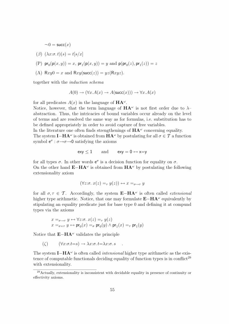
¬ 0 = succ(x)
(β) (λx:σ. t)(s) = t[s/x]
(P) pr0(p(x, y)) = x, pr1(p(x, y)) = y and p(pr0(z), pr1(z)) = z
(A) Rxy0 = x and Rxy(succ(z)) = yz(Rxyz).
together with the induction schema
A(0) → (∀x.A(x) → A(succ(x))) → ∀x.A(x)
for all predicates A(x) in the language of HAω.Notice, however, that the term language of HAω is not first order due to λ–abstraction. Thus, the intricacies of bound variables occur already on the levelof terms and are resolved the same way as for formulas, i.e. substitution has tobe defined appropriately in order to avoid capture of free variables.In the literature one often finds strengthenings of HAω concerning equality.The system I−HAω is obtained from HAω by postulating for all σ ∈ T a functionsymbol eσ : σ→σ→0 satisfying the axioms
exy ≤ 1 and exy = 0 ↔ x=y
for all types σ. In other words eσ is a decision function for equality on σ.On the other hand E−HAω is obtained from HAω by postulating the followingextensionality axiom
(∀z:σ. x(z) =τ y(z)) ↔ x =σ→τ y
for all σ, τ ∈ T . Accordingly, the system E−HAω is often called extensionalhigher type arithmetic. Notice, that one may formulate E−HAω equivalently bystipulating an equality predicate just for base type 0 and defining it at compundtypes via the axioms
x =σ→τ y ↔ ∀z:σ. x(z) =τ y(z)x =σ×τ y ↔ pr0(x) =σ pr0(y) ∧ pr1(x) =τ pr1(y)
Notice that E−HAω validates the principle
(ζ) (∀x:σ.t=s) → λx:σ. t=λx:σ. s .
The system I−HAω is often called intensional higher type arithmetic as the exis-tence of computable functionals deciding equality of function types is in conflict29
with extensionality.
29Actually, extensionality is inconsistent with decidable equality in presence of continuity oreffectivity axioms.
55

When discussing Godel’s functional (“Dialectica”) interpretation one notices (see[Tr73]) that it does not validate the extensionality axiom (∀z:σ. x(z) =τ y(z)) →x =σ→τ y. But it works for I−HAω a shown in [Tr73]. Since the decidabil-ity of higher type equality may appear as undesirable form a mathematicalpoint of view the problem can be remedied also by considering a weaker ver-sion of E−HAω called WE−HAω which we describe next. The language ofWE−HAω is different from the language of HAω in that we only assume anequality predicate for base type 0 and define equality for compomd types interm of this basic equality. For ease of exposition we omit product types whendiscussing WE−HAω. For type σ ≡ σ1 → . . . σn → 0 we define x =σ y as∀z1:σ1, . . . , zn:σn. xz1 . . . zn = yz1 . . . zn. Furthermore one has to work with typedcombinators K and S instead of λ-abstraction and has to reformulate correspond-ing conversion rules of the form t =σ s as tz1 . . . zn = sz1 . . . zn where the zi arefresh variables of type σi. Instead of the extensionality principle for functions weinstead postulate the following weak extensionality rule
P → tz1 . . . zn = sz1 . . . zn(QF-ER)
P → r[t/x] =σ r[s/x]
where P is a quantifier-free formula from which one may derive the rule
P → tz1 . . . zn = sz1 . . . zn(ER)
P → A[t/x] → A[s/x]
where P is still quantifier-free but A is an arbitrary formula and s and t are freefor x in A.
12.2 Models of HAω
Now we will construct some classical models for HAω. First of all there existsthe usual set theoretic model M with
M0 = N Mσ×τ = Mσ ×M τ Mσ→τ = Mσ →M τ
where the constants receive their obvious interpretations. In particular App(f, a) =f(a), i.e. App is interpreted as ordinary function application. This model has thedisadvantage that it contains a lot of non–computable objects. This defect isavoided by the following models.
Hereditary Recursive Operations
By structural recursion over T we define
HRO0 := NHROσ×τ := {e ∈ N | pr0(e) ∈ HROσ ∧ pr1(e) ∈ HROτ}HROσ→τ := {e ∈ N | ∀n ∈ HROσ. {e}(n) ∈ HROτ}
56

App is interpreted as partial recursive application which appears as total due tothe definition of function types. The other codes get their obvious meaning whereR is interpreted by some Godel number for the primitive recursor.This way HRO gets a model for I−HAω when interpreting e as the code ofsome algorithm deciding equality of natural numbers. Moreover, the HRO–modelvalidates Church’s Thesis claiming that all functions of type 0→0 are recursive.
Hereditary Effective Operations
By structural recursion we define a partial equivalence relation ∼σ on N, i.e. asymmetric and transitive but not necessarily reflexive binary relation on N, forevery σ ∈ T via the following clauses
x ∼0 y := x=yx ∼σ×τ y := (pr0(x) ∼σ pr0(y)) ∧ (pr1(x) ∼τ pr1(y))x ∼σ→τ y := ∀z, z′. z ∼σ z
′ → {x}(z) ∼τ {y}(z′)
and we define30
HEOσ := N/∼σ
for σ ∈ T .Now function application is defined as App([e], [n]) = [{e}(n)] and the constantsof HAω get their obvious meaning as in the case of HRO.Notice that HEO is a model of E−HAω due to the way how ∼ is defined forfunction types. But HEO does not model I−HAω as the relations ∼ are notdecidable for function types.
Continuous Function Models
Notice that there are also variants of HRO and HEO based on Baire space Band continuous function application as introduced in Section 11. For exampleone may define in analogy to HRO a hierarchy ICF of Intensional ContinuousFunctionals in the following way
ICF0 := NICF0→0 := BICF0→σ := {α ∈ B | ∀x. (λn.α(〈x〉∗n) ∈ ICFσ)} (σ 6≡ 0)ICFσ→0 := {α ∈ B | ∀β ∈ ICFσ. α(β)↓} (σ 6≡ 0)ICFσ→τ := {α ∈ B | ∀β ∈ ICFσ. α|β ∈ ICFτ} (σ, τ 6≡ 0)
which can be organized into a model of I−HAω. In analogy to HEO one maydefine a hierarchy ECF of Extensional Continuous Functionals which can beorganized into a model of E−HAω.
30If R is a partial equivalence relation on N then we understand N/R as a shorthand for{n∈N|nRn}/R as R is an equivalence relation in the proper sense on the carrier set {n∈N|nRn}of R.
57

13 Kreisel’s Modified Realizability
The basic idea of Kreisel’s Modified Realizability as introduced by him in 1959 isto replace Godel numbers by terms of Godel’s system T . An obvious advantageof this change is that realizers extracted from proofs are already programs (ofGodel’s T ) and, therefore, much easier to grasp and handle than the somewhatawkward Godel numbers. Moreover, such a method works for arbitrary modelsof Godel’s T . Besides these simplifications other a priori unexpected benefits arethat the modified realizability interpretation does not validate Markov’s Principlebut instead the principle of Independence of existence–free Premiss
IPef (A→ ∃x:σ.B(x)) → ∃x:σ. (A→ B(x)) A ∃–free, x 6∈ FV (A)
where a formula is ∃–free if it does not contain occurrences of ∃ and ∨. Thistogether with the axiom of choice for arbitrary types
AC ∀x:σ.∃y:τ.A(x, y) → ∃z:σ→τ.∀x:σ.A(x, z(x))
will give rise to a very convenient axiomatisation of modified realizability.
Now we give the precise definition of modified realizability. We consider A∨B asan abbreviation (or ‘macro’) for ∃n:0. (n=0 → A) ∧ (n 6=0 → B) and, therefore,can omit the clause for disjunction.
Definition 13.1 (Modified Realizability)With every formula A of HAω there is asscoiated a type tp(A) of potential real-izers via the following clauses
tp(t=s) = 0
tp(A∧B) = tp(A)× tp(B)
tp(A→B) = tp(A) → tp(B)
tp(∀z:σ.A) = σ → tp(A)
tp(∃z:σ.A) = σ × tp(A) .
The modified realizability relation xmrA with x of type tp(A) is defined by in-duction on the structure of A via the following clauses
xmr t=s ≡ t=s
xmrA ∧B ≡ pr0(x)mrA ∧ pr1(x)mrB
xmrA→ B ≡ ∀y:tp(A). ymrA→ x(y)mrB
xmr∀z:σ.A(z) ≡ ∀z:σ. x(z)mrA(z)
xmr∃z:σ.A(z) ≡ pr1(x)mrA(pr0(x)) .
The predicate xmrA specifies the actual realizers of A within the type tp(A) ofpotential realizers of A. ♦
58

Notice that the main difference between modified realizability and Kleene’s num-ber realizability (besides the nature of the realizers) is that an actual realizerof A→B has to send potential realizers of A to potential realizers of B besidessending actual realizers of A to actual realizers of B.To get familiar with the notion and for subsequent use let us consider what itmeans that xmr¬A. As ¬A ≡ A→ ⊥ we have xmr¬A ≡ ∀y:tp(A). ymrA→x(y)mr⊥ ≡ ∀y:tp(A). ymrA → ⊥ ≡ ∀y:tp(A).¬ ymrA. Thus, ymrA islogically equivalent to ¬∃y. ymrA.
Next we prove a Soundness Theorem for Modified Realizability.
Theorem 13.1 (Soundness for Modified Realizability)If HAω proves A then there is a term t of type tp(A) such that HAω provestmrA.
Proof: We prove more generally that for every sequence Γ ` A derivable in HAω
there is a term t of type tp(A) such that
~umrΓ ` tmrA
is derivable in HAω where ~umrΓ stands for u1 mrA1∧. . .∧un mrAn. Moreover,the free variables of t are contained in FV (Γ, A)∪{u1, . . . , un}. This generalisedclaim is proved by induction on the structure of derivations in HAω.The cases of structural rules are trivial and, therefore, left to the reader.(∧I) If HAω proves ~umrΓ ` tmrA and ~umrΓ ` smrB then ~umrΓ `p(t, s)mrA∧B.(∧R) If HAω proves ~umrΓ ` tmrA∧B then HAω proves ~umrΓ ` pr0(t)mrAand ~umrΓ ` pr1(t)mrB.(→ I) If HAω proves ~umrΓ ∧ umrA ` tmrB then HAω proves ~umrΓ `λu.tmrA→B.(→ E) If HAω proves ~umrΓ ` tmrA→B and ~umrΓ ` smrA then HAω
proves ~umrΓ ` t(s)mrB.(⊥E) Suppose that HAω proves ~umrΓ ` tmr⊥. Then as tmr⊥ ≡ ⊥ it followsthat HAω proves ~umrΓ ` ⊥ and, therefore, also ~umrΓ ` 0tp(A) mrA.(∀I) If HAω proves ~umrΓ ` tmrA(x) and x does not occur in Γ then HAω
proves ~umrΓ ` λx.tmr∀x.A(x).(∀E) If HAω proves ~umrΓ ` tmr∀x:σ.A(x) then it follows that HAω proves~umrΓ ` t(s)mrA(s) for all terms s of type σ.(∃I) If HAω proves ~umrΓ ` tmrA(s) then it follows that HAω proves ~umrΓ `p(s, t)mr∃x.A(x) as p(s, t)mr∃x.A(x) ≡ pr1(p(s, t))mrA(pr0(p(s, t))) and HAω
proves pr0(p(s, t)) = s and pr1(p(s, t)) = t.(∃E) Suppose as induction hypotheses that HAω proves ~umrΓ ` tmr∃x.A(x)and ~umrΓ ∧ vmrA(x) ` smrB where x is not free in Γ or B. Then as bydefinition tmr∃x.A(x) ≡ pr1(t)mrA(pr0(t)) it follows from the first inductionhypothesis that
59

(1) ~umrΓ ` pr1(t)mrA(pr0(t))
can be proved in HAω. From the second induction hypothesis it follows that
(2) ~umrΓ ∧ pr1(t)mrA(pr0(t)) ` s[pr0(t), pr1(t)/x, v]mrB
can be proved in HAω. As (1) and (2) can be proved in HAω it follows by purelylogical reasoning that ~umrΓ ` s[pr0(t), pr1(t)/x, v]mrB can be proved in HAω.(Axioms) For very equational axiom t=s of HAω it proves 0mr t=s. Fur-thermore, HAω proves that λx:0.0mr¬ 0=succ(x). Let A(0) → (∀x.A(x) →A(succ(x))) → ∀x.A(x) be an instance of the induction schema. Then HAω
provesRtp(A) mrA(0) → (∀x.A(x) → A(succ(x))) → ∀x.A(x)
as from umrA(0) and ∀x:0.∀u:tp(A). umrA(x) → v(x)(u)mrA(succ(x))) onecan derive via the induction principle of HAω that ∀x:0. RuvxmrA(x). 2
Next we are heading for an axiomatization of Modified Realizability for which weneed the following notion.
Definition 13.2 A formula A of HAω is ∃–free iff it does not contain occur-rences of ∃ and, therefore, also not of ∨. ♦
Notice that all formulas of the form xmrA are ∃–free.
Lemma 13.1 For every ∃-free formula A of HAω
(1) (∃x:tp(A). xmrA) → A is provable in HAω and
(2) A→ 0tp(A) mrA is provable in HAω.
Proof: We prove (1) and (2) simultaneously by induction on the structure of A.Notice also that condition (1) for A is logically equivalent to xmrA→ A.If A is an atomic formula then (1) and (2) are obvious as ∃x. xmrA and 0mrAare provably equivalent to A itself.(∧) In HAω one can show that ∃x. xmrA∧B is equivalent to ∃x. xmrA ∧∃x. xmrB. As by induction hypothesis HAω proves ∃x. xmrA → A and∃x. xmrB → B it follows that ∃x. xmrA∧B → A∧B, i.e. that A∧B satis-fies (1). As by induction hypothesis HAω proves A → 0tp(A) mrA and B →0tp(B) mrB it follows that HAω proves A∧B → p(0tp(A), 0tp(B))mrA∧B. As0tp(A∧B) ≡ p(0tp(A), 0tp(B)) we have that HAω proves A∧B → 0tp(A∧B) mrA∧B,i.e. that A∧B satisfies (2).(→) Suppose as induction hypotheses that A and B satisfy the conditions (1)and (2). As by definition xmrA→B ≡ ∀y. ymrA → x(y)mrB and HAω
proves A→ 0tp(A) mrA by induction hypothesis it follows that HAω proves alsoxmrA→B → A → x(0tp(A))mrB and, therefore, also xmrA→B → A → B
60

as by induction hypothesis HAω proves x(0tp(A))mrB → B. Thus, in HAω
one can prove ∃x. xmrA→B → A→B, i.e. A→B satisfies (1). As by defini-tion 0tp(A→B) ≡ λx:tp(A). 0tp(B) HAω proves that 0tp(A→B) mrA→B is equiva-lent to ∀x:tp(A). (xmrA → 0tp(B) mrB) and hence also to ∃x:tp(A). xmrA →0tp(B) mrB. As by induction hypothesis HAω proves ∃x. xmrA → A andB → 0tp(B) mrB it follows that HAω proves (A→B) → (∃x:tp(A). xmrA) →0tp(B) mrB hence (A→B) → 0tp(A→B) mrA→B. Thus A→B satisfies (2) asdesired.(∀) Assume as induction hypothesis that A(z) satisfies (1) and (2). By definitionxmr∀z:σ.A(z) ≡ ∀z:σ. x(z)mrA(z). As by induction hypothesis HAω provesx(z)mrA(z) → A(z) it follows that HAω proves xmr∀z:σ.A(z) → ∀z:σ.A(z)from which it follows immediately that ∀z:σ.A(z) satisfies (1). By inductionhypothesis HAω proves A(z) → 0tp(A(z)) mrA(z) and hence also ∀z.A(z) →∀z.0tp(A(z)) mrA(z). Thus, as by definition 0∀z:σ.A(z) ≡ λz:σ.0tp(A(z)) it followsthat HAω proves ∀z.A(z) → 0∀z:σ.A(z) mr∀z.A(z). Thus ∀z.A(z) satisfies (2). 2
Corollary 13.1 For every formula A of HAω
(1) ∃x. xmr (∃y. ymrA) ↔ ∃y. ymrA is provable in HAω
(2) A ↔ ∃x. xmrA is provable in HAω iff HAω proves that A is equivalentto an existential quantification of an ∃–free formula in HAω.
Proof: (1) By definition xmr (∃y. ymrA) ≡ pr1(x)mr (pr0(x)mrA). As theformula pr0(x)mrA is ∃–free it follows from Lemma 13.1(1) that HAω provespr1(x)mr (pr0(x)mrA) → pr0(x)mrA and, therefore, also xmr (∃y. ymrA) →∃y. ymrA. Thus, HAω proves ∃x. xmr (∃y. ymrA) → ∃y. ymrA. As ymrA is∃–free it follows by Lemma 13.1(2) that HAω proves ymrA→ 0y mrA mr (ymrA)and, therefore, also ymrA → p(y, 0y mrA)mr (∃y. ymrA). Thus, it followsthat HAω proves ymrA→ ∃x. xmr (∃y. ymrA) and, therefore, also that HAω
proves ∃y. ymrA→ ∃x. xmr (∃y. ymrA).(2) The implication from left to right is immediate as xmrA is ∃–free. Forthe reverse direction first observe that it follows (almost) immediately from theSoundness Theorem 13.1 that if HAω proves A1 ↔ A2 then HAω proves also∃x. xmrA1 ↔ ∃x. xmrA2. Thus, it suffices to show for ∃–free formulas B(y)that HAω proves ∃y.B(y) ↔ ∃x. xmr (∃y.B(y)).From Lemma 13.1(2) it follows that HAω proves B(y) → 0tp(B(y)) mrB(y) and,therefore, also B(y) → p(y, 0tp(B(y)))mr∃y.B(y). Thus, HAω proves B(y) →∃x. xmr∃y.B(y) and hence also ∃y.B(y) → ∃x. xmr∃y.B(y).On the other hand by definition xmr∃y.B(y) ≡ pr1(x)mrB(pr0(x)) and fromLemma 13.1(1) it follows that HAω proves pr1(x)mrB(pr0(x)) → B(pr0(x)) as Bis ∃–free by assumption. Thus, HAω proves pr1(x)mrB(pr0(x)) → ∃y.B(y) and,
61

therefore, also xmr∃y.B(y) → ∃y.B(y). Hence HAω proves ∃x. xmr∃y.B(y) →∃y.B(y). 2
Theorem 13.2 (Axiomatization of Modified Realizability)For arbitrary formulas A of HAω
(1) HAω + AC + IPef ` A ↔ ∃x. xmrA
(2) HAω + AC + IPef ` A iff HAω ` tmrA for some term t of type tp(A).
Proof: Claim (1) is proved by induction on the structure of A.For basic formulas claim (1) is obviously true.(∧) This case is trivial as already in HAω ∃x. xmrA ∧ ∃x. xmrB is provablyequivalent to ∃x. xmrA∧B.(→) Assume as induction hypothesis that HAω + AC + IPef proves that A ↔∃y. ymrA and B ↔ ∃z. zmrB. Thus, by AC and IPef (as xmrA is ∃–free) one can show that A→B is equivalent to ∃x.∀y. ymrA → x(y)mrB, i.e.∃x. xmrA→B.(∀) Assume as induction hypothesis that HAω + AC + IPef proves that A(z) ↔∃y. ymrA(z). Thus, using AC one can show that HAω + AC + IPef proves theequivalence of ∀z. A(z) and ∃x.∀z. x(z)mrA(z), i.e. ∃x. xmr∀z. A(z).(∃) Suppose as induction hypothesis that (1) holds for A(z). We have to showthat (1) also holds for ∃z:σ.A(z).Obviously, one can derive already in HAω that xmrA(z) → p(x, z)mr∃z:σ.A(z)from which it follows already in constructive predicate logic that xmrA(z) →∃x. xmr∃z:σ.A(z) and hence that ∃x. xmrA(z) → ∃x. xmr∃z:σ.A(z). Butas by assumption we have that HAω + AC + IPef ` A(z) → ∃x. xmrA(z) itfollows that HAω + AC + IPef ` A(z) → ∃x. xmr∃z:σ.A(z) and, therefore, alsoHAω + AC + IPef ` ∃z.A(z) → ∃x. xmr∃z:σ.A(z).By induction hypothesis one can derive in HAω + AC + IPef that ymrA(z) →A(z) for y 6∈ FV (A) and, therefore, also that ymrA(z) → ∃z.A(z). Substitutingpr0(x) and pr1(x) for z and y, respectively, we get that HAω + AC + IPef provespr1(x)mrA(pr0(x)) → ∃z.A(z) and, therefore, also xmr∃z.A(z) → ∃z.A(z), i.e.∃x. xmr∃z.A(z) → ∃z.A(z).
(2) If HAω ` tmrA then HAω and, therefore, also HAω + AC + IPef prove∃x. xmrA. From this it follows by the already established claim (1) that HAω +AC + IPef ` A.For the reverse direction first observe (exercise!) that one can construct for eachinstance C of AC and IPef a term t such that HAω ` tmrC. If HAω+AC+IPef `A then there exist instances C1, . . . , Cn of AC or IPef such that HAω ` C1 →. . .→ Ck → A. By the Soundness Theorem for Modified Realizability there is a
62

term t with HAω ` tmrC1→ . . .→Ck→A. Let ti be a term with HAω ` ti mrCi
for i = 1, . . . , k. Then obviously HAω ` t(t1) . . . (tk)mrA as desired. 2
From this characterization it follows that HAω + AC + IPef actually proves thefollowing strengthening of IPef
IP (¬A→ ∃y.B(y)) → ∃y.(¬A→ B(y)) y 6∈ FV (A)
where A is an arbitrary formula.
Corollary 13.2 In HAω + AC + IPef one can derive all instances of IP.
Proof: Let A and B(y) be arbitrary formulas of HAω with y 6∈ FV (A). ByTheorem 13.2 in HAω + AC + IPef one can prove the equivalence of A and∃x. xmrA and hence also the equivalence of ¬A and ∀x.¬xmrA. Thus, forshowing that HAω + AC + IPef proves (¬A → ∃y.B(y)) → ∃y.(¬A → B(y)) itsuffices to show that HAω + AC + IPef proves ((∀x.¬xmrA) → ∃y.B(y)) →∃y.((∀x.¬xmrA) → B(y)). But, this trivially is the case as the formula((∀x.¬xmrA) → ∃y.B(y)) → ∃y.((∀x.¬xmrA) → B(y)) is an instance ofIPef because ∀x.¬xmrA is ∃–free. 2
Next we show via modified realizability—as already announced—that in HAω
one cannot derive Markov’s Principle.
Theorem 13.3 (Independence of Markov’s Principle)Relative to HAω + AC + IPef Markov’s Principle MPPR is inconsistent withChurch’s Thesis
CT ∀f :0→0.∃x:0.∀y:0. f(y)={x}(y) .
Thus, in HAω one cannot prove MPPR nor its modified realizability.
Proof: From the previous Corollary 13.2 we know that HAω + AC + IPef provesIP. Assume that ¬¬∃y. T (x, x, y) → ∃y.T (x, x, y) which is an instance of MPPR
as Kleene’s T–predicate is primitive recursive. Then from IP it follows that∀x.∃y.¬¬∃y. T (x, x, y) → T (x, x, y). Thus, by AC it follows that
∃f :0→0.∀x:0.¬¬∃y. T (x, x, y) → T (x, x, f(x))
and, therefore, also
∃f :0→0.∀x:0.¬T (x, x, f(x)) → ¬∃y. T (x, x, y)
by contraposition. Thus, we have
∃f :0→0.∀x:0. T (x, x, f(x)) ↔ ∃y.T (x, x, y)
63

from which it follows that K={x|∃y.T (x, x, y)} is decided by the function g withg(x)=0 iff T (x, x, f(x)). But as such a g cannot be recursive we have shown thatHAω + AC + IPef + MPPR proves the negation of Church’s Thesis.If HAω proves MPPR or its modified realizability then HAω + AC + IPef provesthe modified realizability of MPPR and, therefore, also MPPR itself by Theo-rem 13.2(1). Thus, it follows that HAω + AC + IPef ` ¬CT and, therefore, byTheorem 13.2(2) that HAω ` ∃x. xmr¬CT. But as ∃x. xmr¬CT is provablyequivalent to ¬∃x.xmrCT it follows that HAω ` ¬∃x.xmrCT which is impos-sible as HAω +CT ` ∃x.xmrCT and HRO and HEO are models for HAω +CT.
2
We remark that the underivability of MPPR in HAω can be shown more directlywithout using Corollary 13.2. Suppose that HAω proves ¬¬∃y. T (x, x, y) →∃y.T (x, x, y). Then by the Soundness Theorem 13.1 there is a term t for whichHAω proves tmr¬¬∃y.T (x, x, y)→∃y.T (x, x, y). We leave it as an exerciseto show that from this t one may construct a closed term t for which HAω
proves ∀x.¬¬∃y. T (x, x, y) → T (x, x, t(x)) and thus also ∀x.(∃y.T (x, x, y) ↔T (x, x, t(x)). But this program t would decide the halting problem which isknown to be impossible.
We conclude this section by noticing that just as for number realizability one maydefine a variant of modified realizability “combining it with truth”, i.e. one definesa relation xmrtA just as in Definition 13.1 but with the clause for implicationreplaced by
xmrtA→B ≡ (∀y:tp(A). ymrtA→ x(y)mrtB) ∧ (A→B) .
This modification allows one to prove in HAω that
∃x. xmrtA→ A
for all propositions A. This allows one to establish the following metamathemat-ical facts.
Theorem 13.4 (Applications of Modified Realizability combined with Truth)Let H be one of the systems HAω, I−HAω, E−HAω possibly extended by theprinciples AC and/or IPef . Then
(1) H is consistent relative to HAω.
(2) For closed A and B it follows from H ` A∨B that H ` A or H ` B.
(3) If H ` ∃x.A(x) then H ` A(t) for some term t with FV (t) ⊆ FV (∃x.A(x)).
(4) If H ` ∀x:σ.∃y:τ.A(x, y) then H ` ∃z:σ→τ.∀x:σ.A(x, z(x)).
(5) If H ` A→∃x.B(x) then H ` ∃x.(A→B(x)) if A is ∃–free and x 6∈ FV (A).
64

14 Godel’s Functional Interpretation
Already in 1941 Kurt Godel has devised a method for proof extraction by as-sociating constructive functionals as witnesses or realizers to proofs in HA orHAω. It was not until 1958 that this work was published (in German31) in thephilosophical journal Dialectica under the title “Uber eine bisher nicht benutzteErweiterung des finiten Standpunktes”. That is the reason why Godel’s func-tional interpretation has become known under the name “Dialectica interpreta-tion”. According to the foundationalist ideology which was still32 very influentialin the 40ies and 50ies as a consequence of the Grundlagenkrise of the time be-tween the two World Wars Godel ‘sold’ his functional interpretation of arithmeticas a consistency proof. But, actually, its relevance rather is that it allows one toextract from proofs programs in Godels’s T which was introduced by him for thispurpose. Though Godel’s Functional Interpretation is the oldest such techniqueit appears as the most complex in this vein. But, despite its intriguing characterand inherent (conceptual) complexity it is still of quite some interest because itsimultaneously validates a strong form of Markov’s Principle and a sufficientlystrong version of the principle of Independence of Premiss.The basic idea of Godel’s Functional Interpretation is to associate with everyproposition A a proposition AD ≡ ∃x.∀u.AD(x, u) where AD(x, u) is a primitiverecursive(sic!) relation between x and u of appropriate finite type. One maythink of x as a ‘strategy’ and u as a ‘counterstrategy’ and of AD(x, u) as “x winsagainst u”.In order to simplify notation instead of x and u we consider finite lists x and u
of variables of appropriate type.33 We use x, y, z, u, v,w,X,Y,Z,U,V,W . . . asmeta–variables for finite list of variables and s, t as metavariables for finite listsof terms. If t ≡ t1, . . . , tn then we write ts as an abbreviation for t1s, . . . , tnswhenever the tis are well–formed. Moreover, if x ≡ x1, . . . , xn then we write ∀xand ∃x as shorthand for ∀x1. . . .∀xn. and ∃x1. . . .∃xn. , respectively.Next we consider how the implication ∃x.∀u.AD(x, u) → ∃y.∀v.BD(y, v) can be
31An English translation of this paper can be found in Godel’s Collected Works published byOxford University Press
32This situation changed dramatically in the 60ies under the influence of G. Kreisel whostrongly propagated the view that the significance of the proof–theoretic techniques developedfor ‘foundationalist’ purposes does not lie in their contribution to these very “foundations”.His argument was that consistency proofs for, say, arithmetic use principles more dubious thanthose postulated by arithmetic itself. For example Gentzen used ε0–induction to show theconsisteny of induction over natural numbers! This necessarily has to be case as by Godel’s2nd Incompleteness Theorem no formal system containing a modicum of arithmetic can proveits own consisteny. Instead, as Kreisel emphasized, the relevance of proof–theoretic methodsis that they provide techniques for explicitating or “unwinding” (as he preferred to say) theconstructive contents of formal proofs like algorithms or bounds.
33This notational trick could have been used in the formalization of modified realizability,too. It would have had the nice effect that for ∃–free formulas A we would get xmrA ≡ Awhen defining xmrP ≡ P for atomic P .
65

transformed into an equivalent formula of the form ∃z.∀w.(A→B)D(z,w) as mo-tivation for the subsequent definition of functional interpretation of implications.We have
∃x.∀u.AD(x, u) → ∃y.∀v.BD(y, v) ↔∀x.(∀u.AD(x, u) → ∃y.∀v.BD(y, v)) ↔∀x.∃y.(∀u.AD(x, u) → ∀v.BD(y, v)) ↔∀x.∃y.∀v(∀u.AD(x, u) → BD(y, v)) ↔∀x.∃y.∀v.∃u(AD(x, u) → BD(y, v)) ↔∃Y,U.∀x, v.(AD(x,Uxv) → BD(Yx, v))
where the second and the fourth equivalence are valid only classically and the fifthequivalence presupposes AC. In principle classical logic would permit other waysof prenexing but the ensuing functional interpretations would not be sufficientlywell–behaved w.r.t the purposes of program instruction.As for atomic formulas P we want to put PD ≡ P we have to restrict considerationto systems like I−HAω or WE−HAω where atomic formulas are decidable34. Inthe following we use H as a variable ranging over {I−HAω,WE−HAω}.
Definition 14.1 (Godel’s Functional Interpretation)For atomic formulas P we put
PD ≡ PD ≡ P
and if AD ≡ ∃x.∀u. AD(x, u) and BD ≡ ∃y.∀v. BD(y, v) then we put
(A∧B)D ≡ ∃xy.∀uv. (A∧B)D(x, y, u, v) where(A∧B)D(x, y, u, v) ≡ AD(x, u)∧BD(y, v)
(A→B)D ≡ ∃YU.∀xv. (A→B)D(Y,U, x, v) where(A→B)D(Y,U, x, v) ≡ AD(x,Uxv)→BD(Yx, v)
(∀z.A(z))D ≡ ∃X.∀zu. (∀z.A(z))D(X, z, u) where(∀z.A(z))D(X, z, u) ≡ AD(z,Xz, u)
(∃z.A(z))D ≡ ∃zx.∀u.∃z.A(z))D(z, x, u) where(∃z.A(z))D(z, x, u) ≡ AD(z, x, u) .
We say that functional interpretation validates A iff H ` ∃x.∀u.AD(x, u). ♦
34We shall see subsequently that decidability of AD is needed for showing that A→A∧A isvalidated by functional interpretation in the sense of Definition 14.1. But, moreover, there areformulas provable in HAω which are not validated by functional interpretation as for example∀u, v: 0→0.¬∀z: 0.¬(z=0↔x=y). This formula is provable in HAω as it appears as the ¬¬–translation of ∀u, v: 0→0.∃z: 0.(z=0↔x=y) which, obviously, is provable in HAω + PEM. Butif ∀u, v: 0→0.¬∀z: 0.¬(z=0↔x=y) were validated by functional interpretation there would exista closed term of type 2 deciding whether ¬x=y or ¬¬x=y. But this is impossible as otherwiseequality of total recursive functions were decidable.
66

As in arithmetic A∨B may be considered as an abbreviation for the formula∃n. (n=0→A)∧(n 6=0→B) whose functional interpretation is given by
(A∨B)D ≡ ∃nxy.∀uv. (A∨B)D(n, x, y, u, v) where(A∨B)D(n, x, y, u, v) ≡ (n=0→AD(x, u))∧(n 6=0→BD(y, v)) .
Next we consider how functional interpretation treats negations. As by definition¬A ≡ A→⊥ we have
(¬A)D ≡ ∃U.∀x.¬AD(x,Ux)
when AD ≡ ∃x.∀u.AD(x, u). Thus, as special cases we get
(¬A)D ≡ ∀x.¬AD(x)
if u is empty and(¬A)D ≡ ∃u.¬AD(u)
if x is empty. Accordingly, we have
(¬¬∃x.P (x))D ≡ ∃x.¬¬P (x)
for every atomic formula P (x) as (¬∃x.P (x))D ≡ ∀x.¬P (x). As a consequencewe get that a rather strong form of Markov’s principle is validated by functionalinterpretation.
Lemma 14.1 Functional interpretation validates
M′ ¬¬∃x.P (x) → ∃x.P (x) for P (x) atomic.
Proof: Immediate from the fact that (¬¬∃x.P (x))D ≡ ∃x.¬¬P (x) is provablyequivalent to ∃x.P (x) as P (x) is decidable and hence ¬¬–closed. 2
This together with the following lemma will be useful for axiomatizing FunctionalInterpretation.
Lemma 14.2 Functional interpretation validates
IP′0 (∀x.P (x)→∃y.A(y)) → ∃y.(∀x.P (x)→A(y)) for P (x) atomic.
Proof: Let A(y)D ≡ ∃u.∀v.AD(y, u, v). As (∀x.P (x))D ≡ ∀x.P (x) we observe thatboth (∀x.P (x)→∃y.A(y))D and (∃y.(∀x.P (x)→A(y)))D are syntactically equal to∃y, u,X.∀v. (AD(Xv)→BD(y, u, v)) from which it readily follows that functionalinterpretation validates the schema IP′
0. 2
Functional interpretation is sound in the following sense.
Theorem 14.1 (Soundness of Functional Interpretation)If H ` A then there is a list t of terms such that H ` ∀u.AD(t, u).
67

Proof: As usual we proceed by induction on the structure of derivations in H.Almost everything goes through without any surprises. The only exception is theverification of the correctness of the contraction rule. This requires to show thatfor every formula A functional interpretation validates A→A∧A, i.e. we have toshow that there are X1, X2 and Y such that H proves
AD(x,Yxu1u2) → AD(X1x, u1) ∧ AD(X2x, u2) .
The following turns out as a good choice: put X1x = x = X2x and
Yu1u2 =
{u1 if txu1 6= 0u2 if txu1 = 0
where t is a primitive recursive term deciding AD, i.e. txu = 0 iff AD(x, u).Notice that for I−HAω it is no problem to show that the axioms exy ≤ 1 andexy = 0 ↔ x=y have a functional interpretation because they are quantifier-free.For WE−HAω it is easy to verify the correctness of the rule QF-ER becauseits premiss is quantifier-free and its conclusion is equivalent to its functionalinterpretation (because the premiss of the implication is quantifier-free). 2
Notice that we have used intrinsically that the atomic formulas of H are decidableby primitive recursive terms of the language.Moreover, one can show that AD(t, u) can be proved in the quantifier–free frag-ment QF–H of H augmented with an induction rule. Thus, as the proof of theSoundness Theorem 14.1 is purely combinatorial in character and, therefore, canbe performed in a very weak system (as e.g. PRA) it can be considered as a‘finitistic’ reduction of the consistency of H to the consistency of QF–H. Thelatter was considered by Godel as evident due to the constructive nature of thenotion of primitive recursive functionals of finite type. Thus, Godel thought ofhis result as a consistency proof for intuitionistic (and, therefore, also) classicalarithmetic by “essentially35 finitistic” means.
Now we are going to axiomatize functional interpretation which this time willbe easier as there is no need for considering a syntactically restricted class offormulas.
Lemma 14.3 The system H+ AC + IP′0 + M′ proves A↔ ∃x.∀u.AD(x, u) for all
formulas A.
Proof: We proceed by induction on the structure of A. The only crucial case isimplication. Suppose as induction hypothesis that H + AC + IP′
0 + M′ provesA↔ ∃x.∀u.AD(x, u) and B ↔ ∃y.∀v.AD(y, v).
35Hilbert’s notion of ‘finitistic’ did not encompass the notion of primitive recursive functionalsof finite type. But ‘finitistic’ was (and still is) an open concept and Godel definitely thoughtthat it should encompass the primitive recursive functionals of finite type.
68

Then A→B is equivalent to ∃x.∀u.AD(x, u) → ∃y.∀v.BD(y, v) which in turn (usingIP′
0) is equivalent to ∀x.∃y.∀v. (∀u.AD(x, u) → BD(y, v)). Now if we can showthat ∀u.AD(x, u) → BD(y, v) is equivalent to ∃u.(AD(x, u) → BD(y, v)) it followsthat A→B is equivalent to ∀x.∃y.∀v.∃u. (AD(x, u) → BD(y, v)) which by AC isequivalent to (A→B)D.The desired equivalence of ∀u.AD(x, u) → BD(y, v) and ∃u.(AD(x, u) → BD(y, v))can be seen as follows
∀u.AD(x, u) → BD(y, v) ↔ BD(y, v) ∨ (¬BD(y, v) ∧ ¬∀u.AD(x, u)) ↔↔ BD(y, v) ∨ (¬BD(y, v) ∧ ¬∀u.¬¬AD(x, u)) ↔↔ BD(y, v) ∨ (¬BD(y, v) ∧ ¬¬∃u.¬AD(x, u)) ↔ (by M′)↔ BD(y, v) ∨ (¬BD(y, v) ∧ ∃u.¬AD(x, u)) ↔↔ ∃u.(BD(y, v) ∨ (¬BD(y, v) ∧ ¬AD(x, u)) ↔↔ ∃u.(AD(x, u) → BD(y, v))
using intrinsically the decidability of AD and BD. Notice that for applying M′
correctly we have used (implicitly) that the quantifier–free formula ¬AD is equiv-alent to an atomic formula. 2
Now we can axiomatize Godel’s functional interpretation by AC and the principles
IPω0 (∀x. A(x)∨¬A(x)) → (∀x.A(x)→∃y.B(y)) → ∃y.(∀x.A(x)→B(y))
Mω (∀x. A(x)∨¬A(x)) → ¬¬∃x.A(x) → ∃x.A(x)
for arbitrary formulas A and B.
Theorem 14.2 (Axiomatisation of Functional Interpretation)For all formulas A of H we have
(1) H + AC + IPω0 + Mω ` A ↔ ∃x.∀u.AD(x, u)
(2) H + AC + IPω0 + Mω ` A iff H ` ∃x.∀u.AD(x, u) .
Proof: First notice that in H + AC one easily proves the equivalence of IP′0 and
IPω0 and of M′ and Mω as atomic predicates of H are decidable and in H + AC
every decidable predicate can be shown to be equivalent to an atomic predicateas AC guarantees the existence of a decision function. Thus, claim (1) followsimmediately from Lemma 14.3.The direction from right to left of (2) follows immediately from (1). One easilyshows that AC is validated by functional interpretation. As we already knowthat w.r.t. H + AC the principles IPω
0 and Mω are equivalent to IP′0 and M′,
respectively, it follows immediately from the Soundness Theorem 14.1 and theLemmas 14.1 and 14.2 that IPω
0 and Mω are validated by functional interpretation.
69

Thus, the direction from left to right of (2) follows from these observations bythe Soundness Theorem 14.1. 2
We conclude this section by remarking that there exists the so–called Diller–Nahm variant of Godel’s functional interpretation which allows one to get rid ofthe requirement that atomic formulas are decidable and, accordingly, extends toHAω with or without the extensionality principle.
70

References
[Bar] J. Barwise (ed.) Handbook of Mathematical Logic North Holland, 1977.
[BiBr] E. Bishop, D. Bridges Constructive Analysis Grundlehren der mathema-tischen Wissenschaften 279, Springer, 1985.
[Dum] M. Dummett Elements of Intuitionism Oxford University Press, 2000.
[KV] S. C. Kleene, R. Vesley The Foundations of Intuitionistic MathematicsNorth Holland, 1965.
[Sc69] D. Scott A type theoretical alternative to ISWIM, CUCH, OWHY Theo-retical Computer Science 121, pp.411–440, 1993 (Reprint of a manuscriptwritten at Oxford University in 1969).
[Tr73] A. Troelstra (ed.) Metamathematical Investigations of Intuitionistic Arith-metic and Analysis SLNM 344, Springer Verlag, 1973.
[Tr77] A. Troelstra Aspects of Constructive Mathematics pp. 973-1052 of [Bar].
[TvD] A. Troelstra, D. vanDalen Constructivism in Mathematics 2 vol.’s, NorthHolland, 1988.
71