introduction lifshitz - maths.ed.ac.uknpopovic/downloads/pp2005.pdfapplications of h-matrix...
TRANSCRIPT

APPLICATIONS OF H-MATRIX TECHNIQUES IN
MICROMAGNETICS
NIKOLA POPOVIC AND DIRK PRAETORIUS
Abstract. The variational model by Landau and Lifshitz is frequently usedin the simulation of stationary micromagnetic phenomena. We consider thelimit case of large and soft magnetic bodies, treating the associated Maxwellequation exactly via an integral operator P. In numerical simulations of theresulting minimization problem, difficulties arise due to the imposed side-constraint and the unboundedness of the domain. We introduce a possiblediscretization by a penalization strategy. Here, the computation of P is nu-
merically the most challenging issue, as it leads to densely populated matrices.We show how an efficient treatment of both P and the corresponding bilinearform can be achieved by application of H-matrix techniques.
1. Introduction
The simulation of stationary micromagnetic phenomena occurring in static or quasi-static processes is frequently based on a variational model named after Landau andLifshitz. Therein, one minimizes the energy functional
Eα(m) :=
∫
Ω
φ(m) dx−∫
Ω
f ·m dx+1
2
∫
Rd
|∇u|2 dx+ α
∫
Ω
|∇m|2 dx(1)
over some set of admissible vector-valued magnetizations m : Ω → Rd on a bounded
Lipschitz domain Ω ⊂ Rd corresponding to the magnet, with m(x) := 0 for x ∈
Rd\Ω and d = 2, 3. Here, φ ∈ C∞(Rd;R+) is the anisotropy density (depending on
properties of the material on a crystalline level), f ∈ L2(Ω;Rd) denotes an appliedexterior magnetic field, 0 ≤ α ≪ 1 is the exchange parameter, and u is the magneticpotential related to m by Maxwell’s equation
div(−∇u+m) = 0 in D′(Rd).(2)
The model is completed by adding the non-convex constraint
|m(x)| = 1 for a.e. x ∈ Ω.(3)
For large and soft magnets, the parameter α in (1) vanishes. In general, the modelthen lacks classical solutions, see [JK90], and hence has to be relaxed either byconsidering measure valued solutions [Ped97] or by convexification [DeS93, Tar95].In fact, for a certain limit configuration of soft-large bodies, E0(m), i.e., (1) withα → 0 can be justified to be the correct model, see [DeS93]. The corresponding
1991 Mathematics Subject Classification. 65K10, 65F30, 65F50, 65N30, 65N38.Key words and phrases. Micromagnetics; Landau-Lifshitz model; Magnetic potential; Finite
element method; Hierarchical matrices; Interpolation.
1

2 NIKOLA POPOVIC AND DIRK PRAETORIUS
convexified problem E∗∗0 is given by
E∗∗0 (m) :=
∫
Ω
φ∗∗(m) dx−∫
Ω
f ·m dx+1
2
∫
Rd
|∇u|2 dx(4)
subject to (2) and
|m(x)| ≤ 1 for a.e. x ∈ Ω.(5)
Here, φ∗∗ is the convexified density defined by
φ∗∗(x) = supϕ(x)
∣∣ϕ : Rd → R convex and ϕ|S ≤ φ
for |x| ≤ 1,(6)
where S =x ∈ R
d∣∣ |x| = 1
denotes the unit sphere. Then, the relaxed problem
reads:
Minimize E∗∗0 over A :=
m ∈ L∞(Ω;Rd)
∣∣ ‖m‖L∞(Ω;Rd) ≤ 1.(7)
In contrast to the ill-posed problem E0, the convexification is well-posed [DeS93,Ped97, CP04b]. In fact, this convexified model provides the mathematical founda-tion of the so-called phase theory in micromagnetics, cf. [HS98].
Remark 1. For uniaxial materials such as cobalt, the anisotropy energy is givenby φ(x) = 1/2
(1− (x ·e)2
), with |x| = 1 and e ∈ R
d a given fixed unit vector called
the easy axis. A direct calculation shows φ∗∗(x) = 1/2∑d
j=2(x · zj)2 for |x| ≤ 1
then, where e, z2, . . . , zd is an orthonormal basis of Rd.
The numerical treatment of the minimization problem related to E∗∗0 was initiated
by [CP01] for d = 2, where the authors treat a simplified model obtained by re-
placing Rd in (2) by a bounded Lipschitz domain Ω containing Ω, and solve for
a potential u ∈ H10 (Ω). Here, as in [CP04b, CP04a, LM92, Ma91, Pra04], (2) is
treated exactly via an integral representation, i.e., u = Lm, where L is a linearconvolution operator. We then set Pm := ∇(Lm), see Theorem 2.1 below, andreformulate the stray field energy contribution in (4) in terms of P. The advantageis that in the resulting model, only one discretization for m is required, e.g., bypiecewise constant functions mh.
From a numerical point of view, the computation of Pm for a given magnetizationis the most challenging issue, since it will lead to densely populated matrices. Theaim of the present work is to show how an efficient numerical treatment of bothP and the induced bilinear form a(·, ·) can be achieved by application of H-matrixtechniques.
Remark 2. The treatment of the convexified model (7) requires the explicit knowl-edge of the convexified anisotropy density φ∗∗, which is, however, in general un-known even for simple φ, cf. [DeS93]. Both the Young measure relaxation proposedin [Ped97] and the corresponding discretization [KP01] avoid the computation ofφ∗∗. Note that as far as the computation of the magnetic potential (2) is concerned,our ideas apply in that setting, as well. Further analysis on stabilized discrete mod-els, as well as a comparison of the various approaches, can be found in the articles[CP01] and [KP01], as well as in the survey monograph by Prohl [Pro01].
The remainder of this paper is organized as follows: in Section 2, we give a fewpreliminaries and present a possible discretization of (7); Section 3 contains someinterpolation results required for the following analysis; Section 4 motivates the
APPLICATIONS OF H-MATRIX TECHNIQUES IN MICROMAGNETICS 3
concept of hierarchical (H- resp. H2-) matrices; in Section 5, we give two differentapproaches for a Galerkin discretization of the potential equation (2) via H-matrixtechniques; Section 6 finally summarizes the results of our numerical experiments.
2. Preliminaries and Discretization
This section is devoted to the reformulation of (7) in terms of the associated Euler-Lagrange equations and introduces a possible discretization by a penalization strat-egy.
2.1. Preliminaries. The following Theorem 2.1 gathers some of the properties ofthe operator P required in the following. Proofs can be found in [Pra04], althoughwe expect the result to be known to the experts.
Theorem 2.1 ([LM92, Ma91, Pra04]). Given any m ∈ L∞(Ω;Rd), there exists an(up to an additive constant) unique magnetic potential u = Lm ∈ H1
ℓoc(Rd) such
that
∇u ∈ L2(Rd;Rd) and div(−∇u+m) = 0 in D′(Rd).(8)
The (extended) operator P : L2(Rd;Rd) → L2(Rd;Rd), m 7→ ∇(Lm) is an L2 or-thogonal projection. The potential Lm can be represented as a convolution operator
Lm =d∑
j=1
∂G
∂xj∗mj ,(9)
where m = (m1, . . . ,md) is trivially extended [by zero] from Ω to Rd (so that the
convolution is formally well-defined). Here G : Rd\0 → R is the Newtonian
kernel
G(x) :=
1
γ2log |x|, d = 2,
1
(2− d)γd|x|2−d, d > 2
(10)
for x 6= 0, where the constant γd := |S| > 0 denotes the surface measure of the unitsphere (e.g., γ2 = 2π, γ3 = 4π).
Since the energy functional E∗∗0 from (4) is convex and (Gateaux) differentiable,
the minima are equivalently characterized by the corresponding Euler-Lagrangeequations [DeS93]. Thus, problem (RP ) reads: find (λ,m) ∈ L2(Ω) × L2(Ω;Rd)such that
Pm+Dφ∗∗(m) + λm = f a.e. in Ω,(11)
λ ≥ 0, |m| ≤ 1, λ(1− |m|) = 0 a.e. in Ω.(12)
Existence results for (RP ) can be found in [DeS93, Ped97]; in particular, in theuniaxial case the solution to (RP ) is unique.
2.2. The Discretized Problem. Let T = T1, . . . , TN be a finite family of
pairwise disjoint non-empty open sets Tj which satisfy Ω =⋃N
j=1 Tj . The space of
all T -piecewise constant functions is denoted by P0(T ); h ∈ P0(T ) is the mesh-size
4 NIKOLA POPOVIC AND DIRK PRAETORIUS
function, h|T := hT := diam(T ). For f ∈ L2(Ω), let fT ∈ P0(T ) be the T -piecewiseintegral mean given by
fT |T :=1
|T |
∫
T
f dx for all T ∈ T .
The discrete problem (RPε,h) now reads as follows: given a penalization parameterε ∈ P0(T ) with ε > 0, find mh ∈ P0(T )d such that
〈Pmh +Dφ∗∗(mh) + λhmh ; mh〉L2(Ω) = 〈f ; mh〉L2(Ω) for all mh ∈ P0(T )d,
(13)
where λh ∈ P0(T ) is defined by
λh = ε−1 (|mh| − 1)+|mh|
(14)
with (·)+ := max·, 0.
Remark 3. For mh ∈ P0(T )d, the potential Pmh can be computed exactly, asthe associated bilinear form
a(mh, mh) := 〈Pmh ; mh〉L2(Ω) for all mh, mh ∈ P0(T )d(15)
can be evaluated by a closed form formula, cf. Theorem 5.1. The evaluation of Pmh
is, however, computationally demanding, as it typically leads to densely populatedstiffness matrices.
As for the continuous problem, we have existence of discrete solutions and unique-ness in the uniaxial model case, cf. [CP04b]. Moreover, in that case the a priorierror analysis for (RPε,h) from [CP04b] suggests the choice ε = h for the penaliza-tion parameter, as there holds
‖Pm− Pmh‖L2(Rd) + ‖Dφ∗∗(m)−Dφ∗∗(mh)‖L2(Ω)
+ ‖λm− λhmh‖L2(Ω) + ‖ελhmh‖L2(Ω)
≤ C(‖m−mT ‖L2(Ω) + ‖λm− (λm)T ‖L2(Ω) + ‖ελm‖L2(Ω)
)
with a generic constant C ≥ 0. For (λ,m) sufficiently smooth (e.g., m ∈ H1(Ω;Rd),λm ∈ H1(Ω;Rd)), the above right-hand side turns out to be of order O(ε+ h).
The stiffness matrix A induced by the bilinear form a(·, ·) from (15) will in the
following be approximated by an appropriate H2-matrix A. Given (RPε,h), one
then obtains an approximate discrete model (RP ε,h) after replacing A by A anddefining the approximate bilinear form a(·, ·) accordingly.
3. Multidimensional Interpolation of Integral Kernels
The following section contains some results on the multidimensional interpolationof integral kernels. We restrict ourselves to one particular class of kernel functionshere, known as asymptotically smooth kernels.
APPLICATIONS OF H-MATRIX TECHNIQUES IN MICROMAGNETICS 5
3.1. Asymptotically Smooth Kernels. A kernel function
κ : Rd × Rd → R, (x, y) 7→ κ(x, y)(16)
is said to be asymptotically smooth if there exist constants Casm and casm such that
|∂αx ∂
βy κ(x, y)| ≤ Casm(casm|x− y|)−|α|−|β|−s(α+ β)!(17)
for all multi-indices α, β ∈ Nd0 with |α|+ |β| ≥ 1 and some singularity order s ∈ R,
where x, y ∈ Rd with x 6= y.
Example 3.1. For the Newtonian kernel G defined in (10), κ(x, y) := G(x− y) is
asymptotically smooth for any d ≥ 2, with Casm = γ−12 and Casm =
((2 − d)γd
)−1
for d = 2 and d ≥ 3, respectively, and casm = 1, see [Gra01].
Remark 4. Note that the derivatives of an asymptotically smooth kernel κ also
are asymptotically smooth: given κ := ∂αx ∂
βy κ, (17) holds with s = s + |α| + |β|,
casm = casm + ε for ε > 0 arbitrary, and some Casm depending on Casm and ε. Thisis a consequence of
((α+ β) + (α+ β)
)! ≤ Casm c|α|+|β|
asm (α+ β)!
with an (|α|+ |β|)-dependent constant casm. For every choice of casm > 1, there isa Casm > 0 (depending on casm) such that the above inequality holds. One then
sets Casm := CasmCasm and casm := casmcasm, respectively.
3.2. Interpolation Operators in One Dimension. For m ∈ N0, let the spaceof m-th order polynomials in one spatial variable be denoted by Pm, and considerthe interpolation operator
Im : C[−1, 1] → Pm, u 7→m∑
j=0
u(tj)Lj with Lj(t) =
m∏
k=0k 6=j
t− tktj − tk
(18)
acting on the so-called reference element [−1, 1]. Here(Lj(t)
)mj=0
are the Lagrange
polynomials corresponding to the interpolation points (tj)mj=0. Note that Im is a
projection, i.e., linear with I2m = Im.
For m ∈ N0, the Lebesgue constant Λm ∈ R is defined as the operator norm of Im,
Λm := supu∈C[−1,1]
u6=0
‖Imu‖∞,[−1,1]
‖u‖∞,[−1,1].(19)
Clearly, we have Λm ≥ 1. Moreover, we assume that there are constants λ,Cλ ∈ R+
such that
Λm ≤ Cλ(m+ 1)λ.(20)
For Chebyshev interpolation, where tj = cos((2j + 1)π/(2(m + 1))
), this estimate
holds with λ = 1 = Cλ, cf. [Riv84].
For an arbitrary compact interval I := [a, b] ⊂ R, we define the affine transformation
ΦI : [−1, 1] → I, t 7→ 1
2
((a+ b) + t(b− a)
).
The transformed interpolation operator IIm is then given by
IIm : C[a, b] → Pm, u 7→
(Im(u ΦI)
) Φ−1
I .
6 NIKOLA POPOVIC AND DIRK PRAETORIUS
Obviously, the projection property as well as (20) now carry over from Im to IIm.
3.3. Tensor Interpolation Operators. For a family of closed intervals Ij :=[aj , bj ] ⊂ R, j ∈ 1, . . . , 2d, define the axially parallel box B ⊂ R
2d by B :=∏2dj=1 Ij . Given a family
(IIjm
)2dj=0
of interpolation operators on (Ij)2dj=0, the m-th
order tensor product interpolation operator IBm on B is then defined as
IBm := II1
m ⊗ · · · ⊗ II2dm .
In analogy to IIm, IB
m is a projection from C(B) to
Qm := spanp1 ⊗ · · · ⊗ p2d
∣∣ pj ∈ Pm, j ∈ 1, . . . , 2d.(21)
We require the following result on the interpolation error of IBm adapted from [BG04,
BLM04]:
Theorem 3.2. Let u ∈ C∞(B) such that there are constants Cu, γu ∈ R+ satisfying
‖∂nj u‖∞,B ≤ Cuγ
nun!(22)
for all j ∈ 1, . . . , 2d and n ∈ N0. Then, we have
‖u− IBmu‖∞,B ≤ 16edCuΛ
2dm
(1 + γudiam(B)
)(m+ 1)
(1 +
2
γudiam(B)
)−(m+1)
.
(23)
Proof. The proof is as in [BG04, Theorem 3.2], with the d there replaced by 2d.
3.4. Local Error Analysis for Asymptotically Smooth Kernels. We nowapply interpolation to obtain an approximate degenerate kernel κ := IB
mκ insteadof the given asymptotically smooth integral kernel κ. Let Bσ, Bτ ⊂ R
d be compactaxially parallel boxes with positive Euclidean distance dist(Bσ, Bτ ) > 0:
Lemma 3.3. An asymptotically smooth kernel κ : Rd × Rd → R satisfies (22) on
B := Bσ ×Bτ , with constants
Cκ = max
‖κ‖L∞(Bσ×Bτ ),
Casm(casmdist(Bσ, Bτ )
)s
and γκ =
1
casmdist(Bσ, Bτ ).
(24)
Provided diam(Bσ ×Bτ ) ≤ η dist(Bσ, Bτ ) with η > 0, there holds in particular
‖κ− I(σ,τ)m κ‖L∞(Bσ×Bτ ) ≤ c1c2Cκ
(1 +
2casmη
)−(m+1)
(25)
with I(σ,τ)m := IB
m, a numerical constant c1 = 16ed(1 + η/casm), and a constantc2 = Λ2d
m (m+ 1) with only polynomial increase in m.
Remark 5. Note that the constant Cκ > 0 behaves like dist(Bσ, Bτ )−s for the
kernels we are interested in, such as κ(x, y) = log |x− y| resp. κ(x, y) = |x− y|−s.
Proof of Lemma 3.3. Direct computation shows that (22) is valid, and Theorem 3.2yields
‖κ− IBmκ‖L∞(B) ≤ 16ed
(1 + γκdiam(B)
)Λ2dm (m+ 1)Cκ
(1 +
2
γκdiam(B)
)−(m+1)
.
Combining this with γκdiam(B) ≤ η/casm, we obtain (25).
APPLICATIONS OF H-MATRIX TECHNIQUES IN MICROMAGNETICS 7
The proof of Theorem 3.2 is only based on the stability constant Λm defined in (19).The advantage is that the resulting estimate can be applied to a fairly wide range ofinterpolation operators. If one restricts oneself to tensor Chebyshev interpolation– as we will do in the numerical experiments – one can do better by using thefollowing error estimate for tensor Chebyshev polynomials adapted from [BH02]:
Lemma 3.4. Provided diam(Bσ ×Bτ ) ≤ η dist(Bσ, Bτ ) with η > 0, an asymptoti-cally smooth kernel κ on B := Bσ ×Bτ ⊂ R
2d satisfies
‖κ− I(σ,τ)m κ‖∞,B ≤ dCasmc
−sasm Λ2d−1
m dist(Bσ, Bτ )−s 4−mc−(m+1)
asm ηm+1.(26)
Proof. The proof is along the lines of [BH02].
Remark 6. Lemma 3.3 ensures (asymptotically) exponential convergence with re-spect tom irrespective of the choice of η > 0. Nevertheless, the constant c1 obtainedin Lemma 3.3 is too pessimistic, in contrast to the reasonably good approximationresults observed for small m, as well, cf. Section 6. From Lemma 3.4 we obtainexponential convergence provided at least 4casm > η, with the highly improvedconstants c1 = dCasmc
−sasm ≪ 16ed(1 + η/casm) and c2 = Λ2d−1
m ≪ Λ2dm (m+ 1).
In the following, we require additional error estimates for tensor Chebyshev polyno-mials, in particular for the norms of the first and second derivatives of the respectiveinterpolation errors. For the proofs, we make use of the following well-known one-dimensional error estimate for Chebyshev interpolation from [BH02],
‖u− IIjmu‖∞,Ij ≤ 4−m
2(m+ 1)!|Ij |m+1 ‖u(m+1)‖∞,Ij for u ∈ Cm+1(Ij),(27)
as well as of a result on the first derivative of u−Imu in one dimension taken fromthe proof of [BS01, Theorem 3.3.1],
‖(u− Imu)′‖∞,[−1,1] ≤(
1
(r − 1)!+
1
r!C(m)
)‖u(r)‖∞,[−1,1] for u ∈ Cr[−1, 1],
(28)
with 1 ≤ r ≤ m+1 and C(m) a constant which may be estimated by C(m) ≤ Λmm2,cf. [BS01]. Affine transformation then yields
‖(u− Imu)′‖∞,Ij ≤ 2−(r−1)|Ij |r−1
(1
(r − 1)!+
1
r!Λmm2
)‖u(r)‖∞,Ij(29)
for Ij := [aj , bj ] ⊂ R.
Furthermore, we need an estimate for the norms of the derivatives of algebraicpolynomials known as Markov’s Theorem [DL93, Theorem 1.4]:
‖p′‖∞,Ij ≤ m22|Ij |−1‖p‖∞,Ij for p ∈ Pm.(30)
This estimate cannot be improved; in particular, it is sharp for the Chebyshevpolynomials.
To begin with, we state a result concerning the first derivatives of κ− I(σ,τ)m κ.
Lemma 3.5. Provided diam(Bσ ×Bτ ) ≤ η dist(Bσ, Bτ ) with η > 0, an asymptoti-cally smooth κ ∈ Cm+2(B) on B := Bσ ×Bτ satisfies
‖∂α(κ− I(σ,τ)m κ)‖∞,B ≤ c1c22
−mc−(m+1)asm ηm+1 for 1 ≤ α ≤ 2d,(31)
8 NIKOLA POPOVIC AND DIRK PRAETORIUS
where c1 is a numerical constant depending on d, B, and κ and c2 = (Λmm2+m+1)Λ2d−1m grows polynomially in m.
Proof. As in [BG04, BH02], we write
‖∂α(κ− I(σ,τ)m κ)‖∞,B ≤
2d∑
j=1
∥∥∥∥∂α( j−1⊗
k=1
IIkm ⊗ (Id− IIj
m )⊗2d⊗
k=j+1
Id
)κ
︸ ︷︷ ︸=:Jjκ
∥∥∥∥∞,B
;(32)
to obtain estimates for ‖∂αJjκ‖∞,B , we have to consider three cases.
• First, for j < α, an explicit computation gives ∂αJjκ = Jj(∂ακ), whence
‖∂αJjκ‖∞,B ≤ Λj−1m
∥∥∥∥( j−1⊗
k=1
Id⊗ (Id− IIjm )⊗
2d⊗
k=j+1
Id
)∂ακ
∥∥∥∥∞,B
≤ Λj−1m
4−m
2(m+ 1)!|Ij |m+1‖∂m+1
j ∂ακ‖∞,B ;
here we have used (19) on IIkm , k < j, and applied the estimate in (27) to Ij . By
exploiting the asymptotic smoothness of κ to estimate ‖∂m+1j ∂ακ‖∞,B ≤ Casm
(casm
dist(Bσ, Bτ ))−(m+2+s)
(m + 2)!, |Ij | ≤ diam(Bσ × Bτ ), and diam(Bσ × Bτ ) ≤ ηdist(Bσ, Bτ ), we get
‖∂αJjκ‖∞,B ≤ Casmc−(s+1)asm dist(Bσ, Bτ )
−(s+1)c−(m+1)asm ηm+1m+ 2
24−mΛj−1
m .(33)
• Second, for j = α, it follows from (29) with r = m+ 1 that
‖∂αJακ‖∞,B ≤ Λα−1m
∥∥∥∥( α−1⊗
k=1
Id⊗ ∂α(Id− IIαm )⊗
2d⊗
k=α+1
Id
)κ
∥∥∥∥∞,B
≤ Λα−1m 2−m|Iα|m
(1
m!+
m2
(m+ 1)!Λm
)‖∂m+1
α κ‖∞,B .
As before, we now obtain
(34) ‖∂αJακ‖∞,B ≤ Casmc−sasmdist(Bσ, Bτ )
−sc−(m+1)asm ηm+1
× (Λmm2 +m+ 1)2−m|Iα|−1Λα−1m .
• Third, the case j > α is treated by applying Markov’s Theorem (30) to IIαm and
by using the estimate in (27), whence
‖∂αJjκ‖∞,B ≤ Λj−1m m22|Iα|−1
∥∥∥∥( j−1⊗
k=1
Id⊗ (Id− IIjm )⊗
2d⊗
k=j+1
Id
)κ
∥∥∥∥∞,B
≤ Λj−1m m2 4−m
(m+ 1)!|Iα|−1|Ij |m+1‖∂m+1
j κ‖∞,B
and
‖∂αJjκ‖∞,B ≤ Casmc−sasmdist(Bσ, Bτ )
−sc−(m+1)asm ηm+1m24−m|Iα|−1Λj−1
m .(35)

APPLICATIONS OF H-MATRIX TECHNIQUES IN MICROMAGNETICS 9
Collecting the estimates in (33), (34), and (35), we finally have
‖∂α(κ− I(σ,τ)m κ)‖∞,B
≤ Casmdist(Bσ, Bτ )−sc−(m+1)
asm ηm+1c−sasm
(c−1asm
m+ 2
24−mdist(Bσ, Bτ )
−1∑
j<α
Λj−1m
+ (Λmm2 +m+ 1)2−m|Iα|−1Λα−1m +m24−m|Iα|−1
∑
j>α
Λj−1m
)
≤ c−(m+1)asm ηm+1(Λmm2 +m+ 1)2−mΛ2d−1
m Casmc−sasmdist(Bσ, Bτ )
−s
×((α− 1)c−1
asmdist(Bσ, Bτ )−1 +
(2d− (α− 1)
)(min2dj=1|Ij |
)−1),
which gives the desired result.
For the second derivatives of κ− I(σ,τ)m κ, we obtain in a similar fashion:
Lemma 3.6. Under the assumptions of Lemma 3.5, we have
‖∂α∂β(κ− I(σ,τ)m κ)‖∞,B ≤ c1c22
−(m−1)c−(m+1)asm ηm+1 for 1 ≤ α, β ≤ 2d,(36)
with a constant c1 depending on d, B, and κ and c2 = (Λmm2 +m+ 1)m2Λ2d−1m .
Proof. Without loss of generality, we assume 1 ≤ α ≤ β ≤ 2d throughout; similarreasoning as in the proof of Lemma 3.5, with Jjκ defined as in (32), then impliesthe following cases:
• j < α ≤ β: with ∂α∂βJjκ = Jj(∂α∂βκ), one has as in (33)
‖∂α∂βJjκ‖∞,B ≤ Λj−1m
4−m
2(m+ 1)!|Ij |m+1‖∂m+1
j ∂α∂βκ‖∞,B
≤ Λj−1m Casmc
−(s+2)asm dist(Bσ, Bτ )
−(s+2)c−(m+1)asm ηm+14−m (m+ 2)(m+ 3)
2;
• j = α < β: from ∂α∂βJακ = ∂αJα(∂βκ) and (29) for r = m+ 1 it follows that
‖∂α∂βJακ‖∞,B ≤ Λα−1m 2−m|Iα|m
(1
m!+
m2
(m+ 1)!Λm
)‖∂m+1
j ∂βκ‖∞,B
≤ Λα−1m Casmc
−(s+1)asm dist(Bσ, Bτ )
−(s+1)|Iα|−1c−(m+1)asm ηm+12−m
× (m+ 2)(1 +m+m2Λm),
cf. (34);• α < j < β: as ∂α∂βJjκ = ∂αJj(∂βκ), we obtain with (30)
‖∂α∂βJjκ‖∞,B ≤ Λj−1m m22|Iα|−1 4−m
2(m+ 1)!|Ij |m+1‖∂m+1
j ∂βκ‖∞,B
≤ Λj−1m Casmc
−(s+1)asm dist(Bσ, Bτ )
−(s+1)|Iα|−1c−(m+1)asm ηm+14−mm2(m+ 2),
see (35);• j = α = β: to obtain an estimate for ∂2
jJjκ, we proceed as in [BS01, Theorem
3.3.1]: given u ∈ Cm+1[−1, 1] and 1 ≤ r ≤ m+1, let Rr be the remainder term of theTaylor series expansion of degree r−1 of u about t = 0. Using u−Imu = Rr−ImRr,
10 NIKOLA POPOVIC AND DIRK PRAETORIUS
‖Rr‖∞,[−1,1] ≤ 1/r!‖u(r)‖∞,[−1,1], and ‖R′′r‖∞,[−1,1] ≤ 1/(r − 2)!‖u(r)‖∞,[−1,1], we
have by the triangle inequality and with (30)
‖(u− Imu)′′‖∞,[−1,1] ≤ ‖R′′r‖∞,[−1,1] + ‖(ImRr)
′′‖∞,[−1,1]
≤ 1
(r − 2)!‖u(r)‖∞,[−1,1] +m2(m− 1)2Λm
1
r!‖u(r)‖∞,[−1,1].
By affine transformation it follows for u ∈ Cm+1(Iα) and r = m+ 1 that
‖(u− Imu)′′‖∞,Iα
≤ 2−(m−1)|Iα|m−1
(1
(m− 1)!+
1
(m+ 1)!(m− 1)2m2Λm
)‖u(m+1)‖∞,Iα ,
whence
‖∂2αJακ‖∞,B ≤ Λα−1
m
∥∥∥∥( α−1⊗
k=1
Id⊗ ∂2α(Id− IIα
m )⊗2d⊗
k=α+1
Id
)κ
∥∥∥∥∞,B
≤ Λα−1m 2−(m−1)|Iα|m−1
(1
(m− 1)!+
1
(m+ 1)!(m− 1)2m2Λm
)‖∂m+1
α κ‖∞,B
≤ Λα−1m Casmc
−sasmdist(Bσ, Bτ )
−s|Iα|−2c−(m+1)asm ηm+12−(m−1)
×(m(m+ 1) + (m− 1)2m2Λm
);
• α < j = β: with ∂α∂βJβκ = ∂α(∂βJβκ), (29) and (30) give
‖∂α∂βJβκ‖∞,B ≤ Λβ−1m m22|Iα|−12−m|Iβ |m
(1
m!+
m2
(m+ 1)!Λm
)‖∂m+1
β κ‖∞,B
≤ Λβ−1m Casmc
−sasmdist(Bσ, Bτ )
−s|Iα|−1|Iβ |−1c−(m+1)asm ηm+12−(m−1)
×m2(1 +m+m2Λm
);
• α ≤ β < j: applying Markov’s Theorem (30) twice yields
‖∂α∂βJjκ‖∞,B ≤ Λj−1m m22|Iα|−1m22|Iβ |−1 4−m
2(m+ 1)!|Ij |m+1‖∂m+1
j ∂ακ‖∞,B
≤ Λj−1m Casmc
−sasmdist(Bσ, Bτ )
−s|Iα|−1|Iβ |−1c−(m+1)asm ηm+14−(m−1)m
4
2.
Let us first consider α < β: by collecting the above estimates, we obtain as inLemma 3.5
‖∂α∂β(κ− I(σ,τ)m κ)‖∞,B
≤ Casmc−sasmdist(Bσ, Bτ )
−s(Λmm2 +m+ 1)m22−(m−1)Λ2d−1m c−(m+1)
asm ηm+1
×((α− 1)c−2
asmdist(Bσ, Bτ )−2 + (β − α)c−1
asmdist(Bσ, Bτ )−1
(min2dj=1|Ij |
)−1
+(2d− (β − 1)
)(min2dj=1|Ij |
)−2),
from which the result follows. An analogous computation for α = β shows that theestimate then still holds, with the same constants c1 and c2. This concludes theproof.
APPLICATIONS OF H-MATRIX TECHNIQUES IN MICROMAGNETICS 11
Remark 7. Lemmas 3.5 and 3.6 ensure exponential convergence with respect to mprovided at least 2casm > η. For κ the Newtonian kernel G, this implies exponentialconvergence for η ∈ (0, 2), cf. Remark 4.
4. H2-Matrix Techniques
In this section, we motivate the concept of hierarchical matrices and give the cor-responding definitions.
4.1. Motivation. We consider a bilinear form a(·, ·) on L2(Ω) given by a doubleintegration with an asymptotically smooth kernel κ,
a(u, v) :=
∫
Ω
∫
Ω
u(x)κ(x, y)v(y) dy dx for u, v ∈ L2(Ω),(37)
with Ω ⊂ Rd a bounded domain. In the following we require a partition T of Ω and
a block partitioning P of T × T . For η > 0 fixed, a block (σ, τ) ∈ P is then calledadmissible provided
diam(Bσ ×Bτ ) ≤ η dist(Bσ, Bτ ),(38)
where Bσ and Bτ denote axially parallel boxes in Rd of minimal size containing
∪σ and ∪τ , respectively; otherwise (σ, τ) is called inadmissible. Here ∪σ :=x ∈
T∣∣T ∈ σ ⊆ T
(resp. ∪τ :=
y ∈ T
∣∣T ∈ τ ⊆ T) denotes the union of all
elements T ∈ T contained in σ (resp. in τ). P is thus split into two subsets Pfar
and Pnear: the subset of all admissible blocks is called far field and denoted by Pfar;the inadmissible blocks are collected in the near field Pnear := P\Pfar.
The approximate bilinear form a(·, ·) is obtained by replacing the kernel functionon admissible blocks by an approximate but degenerate kernel obtained by inter-polation. More precisely,
(39) a(u, v) :=∑
(σ,τ)∈Pnear
∫
∪σ
∫
∪τ
u(x)κ(x, y)v(y) dy dx
+∑
(σ,τ)∈Pfar
∫
∪σ
∫
∪τ
u(x)(I(σ,τ)m κ(x, y)
)v(y) dy dx,
where I(σ,τ)m denotes the tensor interpolation operator with respect to the bounding
box B := Bσ ×Bτ .
For each τ ⊆ T with corresponding bounding box Bτ , define a family (xτj )
Mτ
j=0
of interpolation points plus the associated tensor Lagrange polynomials (Lτj )
Mτ
j=0,where Mτ ∈ N. Given
I(σ,τ)m κ(x, y) =
Mσ∑
m1=0
Mτ∑
m2=0
κ(xσm1
, xτm2
)Lσm1
(x)Lτm2
(y) for (x, y) ∈ ∪σ × ∪τ,
the second term from (39) can then be written as
∑
(σ,τ)∈Pfar
Mσ∑
m1=0
Mτ∑
m2=0
κ(xσm1
, xτm2
)︸ ︷︷ ︸
=:Sστm1m2
∫
∪σ
u(x)Lσm1
(x) dx
︸ ︷︷ ︸=:V σ
m1(u)
∫
∪τ
v(y)Lτm2
(y) dy
︸ ︷︷ ︸=:V τ
m2(v)
.(40)
12 NIKOLA POPOVIC AND DIRK PRAETORIUS
The advantage of this new representation becomes obvious if we discretize a(·, ·):consider the basis ϕ1, . . . , ϕN of the space P0(T ) of piecewise constant functionson T given by ϕj := χTj
, where χTjis the characteristic function on Tj ∈ T and
N = |T |, and define A ∈ RN×N by Ajk := a(ϕj , ϕk) and the approximate matrix
A ∈ RN×N by Ajk := a(ϕj , ϕk) for all 1 ≤ j, k ≤ N . On inadmissible blocks
(σ, τ) ∈ Pnear, we then simply have A|σ×τ = A|σ×τ , whereas for (σ, τ) ∈ Pfar, A isgiven by
A|σ×τ = V σSστV τ T ≈ A|σ×τ ,(41)
with V σjm1
:= V σm1
(ϕj) and V τkm2
:= V τm2
(ϕk) as defined in (40).
4.2. Block Partitioning. A simple method to find a hierarchical partition P ofT × T is to first construct a cluster tree from T by binary space partitioning: onestarts with the root cluster containing all T ∈ T , splits it into two son clustersand repeats the procedure recursively until each cluster contains less than a givennumber of elements Cℓf . Geometrically speaking, for every T ∈ T , one chooses acoordinate axis and splits the set along this axis.
One can then use the admissibility condition (38) in combination with the clustertree structure to construct P: starting with T × T , one splits each pair of clustersas long as it is not admissible. This gives a P satisfying T × T =
⋃(σ,τ)∈P
σ × τ .
Clearly, a pair (σ, τ) can only appear in P if it is admissible or if either σ or τ is aleaf. The above procedure can easily be formalized, see e.g. [BGH03, BH02, HKS00]for formal definitions and algorithms.
4.3. H-Matrices vs. H2-Matrices. Based on the concepts of cluster tree andblock partitioning, the matrix approximation approach outlined in Section 4.1 canbe generalized by introducing a class of data-sparse matrices, the so-called H-matrices. Given a block partitioning P of T × T and some k ∈ N, a matrix A ∈R
N×N is called H-matrix of rank k provided rank(A|σ×τ ) ≤ k for each (σ, τ) ∈ P.Moreover, if a factorization of the form (41) holds for a family V = (V τ )τ⊆T andsome multiplication matrices Sστ , A is called uniform H-matrix with respect to thecluster basis V , cf. [BGH03, HKS00].
Additional structure can be gained by considering uniform H-matrices for whichthe corresponding cluster bases are nested: if the space Qm defined in (21) is usedfor interpolation on all clusters, polynomials corresponding to father clusters canbe expressed exactly in terms of polynomials corresponding to son clusters. Forτ ⊆ T and τ ′ ∈ sons(τ), we have
Lτj (x) =
M∑
m=0
Lτj
(xτ ′
m
)Lτ ′
m(x).(42)
Defining the transfer matrix Bτ ′τ ∈ RM×M by Bτ ′τ
mj := Lτj
(xτ ′
m
), we obtain
(43) V τij =
∫
∪τ
χTjLτj (x)dx =
∑
τ ′∈sons(τ)
M∑
m=0
Lτj
(xτ ′
m
) ∫
∪τ ′
χTjLτ ′
m(x)dx
=∑
τ ′∈sons(τ)
M∑
m=0
Bτ ′τmj V
τ ′
im
APPLICATIONS OF H-MATRIX TECHNIQUES IN MICROMAGNETICS 13
for all i ∈ τ ′ ⊂ τ , i.e., V τ |τ ′ = V τ ′
Bτ ′τ . A is called H2-matrix with respect to V ifit is a uniform H-matrix with respect to V and if V is nested.
Remark 8. For H2-matrices, one only has to store the multiplication matrices Sστ
for all admissible blocks (σ, τ) ∈ Pfar, the cluster matrices V τ for all leaves τ ⊆ T ,
the transfer matrices Bτ ′τ for all father-son pairs, and A|σ×τ on all non-admissibleblocks (σ, τ) ∈ Pnear.
Remark 9. To evaluate (39), fast and efficient algorithms for matrix-vector multi-plication are required. We assume the underlying partitioning P to be sparse in the
sense of [Gra01], with some sparsity constant Csp. Given an H2-matrix A ∈ RN×N
and x, y ∈ RN , it can then be shown that the computation of y = Ax needs only
O(Nmd) operations to complete. Similarly, both the number of operations requiredto build an H2-matrix approximation and the amount of storage needed to storeit are of order O(Nmd), cf. [BGH03, Gie01, HKS00]. Note that Csp enters allthe above complexity estimates; for Csp → ∞, the complexity of the problem willbecome unbounded, as well. Estimates on Csp can be found in [GH03].
4.4. Global Error Analysis for the Approximate Bilinear Form. By defi-nition of the admissibility condition (38), one can apply the approximation resultsof Section 3.4 on each admissible block (σ, τ) ∈ Pfar. Indeed, given some constantc3, Lemma 3.4 shows that we can choose an approximation order m ∈ N so that
‖κ− I(σ,τ)m κ‖L∞(Bσ×Bτ ) ≤ c3
for all (σ, τ) ∈ Pfar.
Theorem 4.1. Under the above assumptions, we have
|a(u, v)− a(u, v)| ≤ c3‖u‖L1(Ω)‖v‖L1(Ω) ≤ c3|Ω|‖u‖L2(Ω)‖v‖L2(Ω)(44)
for all u, v ∈ L2(Ω).
Proof. For almost all (x, y) ∈ Ω×Ω, we define an integral kernel κ(x, y) as follows.Let S :=
⋃∂T
∣∣T ∈ Tdenote the skeleton of the partition. Note that S ⊂ R
d
is a set of measure zero. For x, y ∈ Ω\S, there are unique elements Tx, Ty ∈ Tsatisfying x ∈ Tx and y ∈ Ty, respectively. Since P is a partition of T × T , there isa unique block (σ, τ) ∈ P with (Tx, Ty) ∈ σ × τ . Consequently, we may define
κ(x, y) :=
κ(x, y) if (σ, τ) is not admissible,
I(σ,τ)m κ(x, y) else.
Since a(·, ·) and a(·, ·) differ only on the far-field blocks, we have
|a(u, v)− a(u, v)| =∣∣∣∣∫
Ω
∫
Ω
u(x)(κ(x, y)− κ(x, y)
)v(y) dy dx
∣∣∣∣ ,
and a Holder inequality yields
|a(u, v)− a(u, v)| ≤ ‖κ− κ‖L∞(Ω×Ω)‖u‖L1(Ω)‖v‖L1(Ω),
since u(x) and v(y) decouple on Ω×Ω. Using ‖u‖L1(Ω) ≤ |Ω|1/2‖u‖L2(Ω), we obtainthe desired estimate.

14 NIKOLA POPOVIC AND DIRK PRAETORIUS
4.5. Global Error Analysis for the Corresponding Matrix. Let Uh ≤ L2(Ω)be a finite-dimensional space, and define the stiffness matrix A ∈ R
N×N and its H2-
approximation A ∈ RN×N by Ajk := a(uj , uk) and Ajk := a(uj , uk), respectively,
for a fixed basis u1, . . . , uN of Uh. Then, there holds
Corollary 4.2. The approximation error for the stiffness matrix A is bounded by
‖A− A‖F ≤ Nc3(maxNj=1‖uj‖L1(Ω)
)2.(45)
In particular, the error decreases exponentially with the approximation order m.
Provided A is a regular matrix, A also is regular for large approximation orders m.
Proof. The first assertion follows by applying Theorem 4.1 to each entry of A.Regularity is immediate, as the regular matrices GL(N) form an open subset ofR
N×N .
5. Galerkin Discretization of the Potential Equation
In this section we provide two differentH2-matrix approaches to obtain a reasonabledata sparse approximation of the stiffness matrix
A ∈ RdN×dN with Ajk := a(ϕj , ϕk)(46)
for a fixed basis ϕ1, . . . , ϕdN of P0(T )d, where the bilinear form a(·, ·) is definedas in (15). We recall a result from [Pra04].
Theorem 5.1. For bounded Lipschitz domains ω, ω ⊂ Rd and vectors m, m ∈ R
d,we have
a(χωm, χωm) = −∫
∂ω
∫
∂ω
G(x− y)(ννν(x) ·m
)(ννν(y) · m
)dsy dsx,(47)
where ννν and ννν denote the outer normal vectors on ∂ω and ∂ω, respectively. Fur-thermore, we have the symmetry properties
a(χωm, χωm) = a(χωm, χωm) = a(χωm, χωm),(48)
and in the case dist(ω, ω) > 0 there holds
a(χωm, χωm) =
∫
ω
∫
ω
m ·HG(x− y)m dy dx(49)
with the Hessian HG of the Newtonian kernel G.
Now, a reasonable choice for a basis of P0(T )d is
ϕj := χTje1, ϕj+N := χTj
e2 etc. for 1 ≤ j ≤ N,(50)
as is shown in the following. This basis gives rise to the definition of the matrices
Aαβ ∈ RN×Nsym for fixed 1 ≤ α, β ≤ d, Aαβ
jk := a(χTjeα, χTk
eβ),(51)
where the symmetry of Aαβ (i.e., an additional symmetry of A) follows from (48).Note that – again by equation (48) – we have Aαβ = Aβα. Therefore, A is asymmetric d× d block matrix with symmetric blocks Aαβ of dimension N ×N ,
A =
(A11 A12
A12 A22
)for d = 2 and A =
A11 A12 A13
A12 A22 A23
A13 A23 A33
for d = 3,
(52)
APPLICATIONS OF H-MATRIX TECHNIQUES IN MICROMAGNETICS 15
respectively. The idea is to approximate each block Aαβ by an appropriate H2-matrix.
5.1. Approximation of A on Far Field Blocks via (49). A direct H2-matrixapproach stems from the far field representation (49) for which the Hessian (i.e.,the second derivatives) of the Newtonian kernel enters,
∂2G
∂xα∂xβ(x) =
1
γd
δαβ |x|2 − dxαxβ
|x|d+2for x ∈ R
d\0,(53)
where 1 ≤ α, β ≤ d and δαβ denotes the Kronecker delta. Obviously, these kernelsare asymptotically smooth with singularity order s = −d, cf. Remark 4. Let P
be a block partitioning with respect to the given triangulation T . To abbreviatenotation, let νννj denote the outer normal vector on the boundary ∂Tj of an element
Tj , and let mjh := mh|Tj
∈ Rd be a discrete magnetization mh ∈ P0(T )d. In
analogy to the previous section and according to (47) and (49), the bilinear forma(·, ·) on P0(T )d reads
(54) a(mh, mh) = −N∑
j,k=1
∫
∂Tj
∫
∂Tk
G(x− y)(νννj(x) ·mj
h
)(νννk(y) · mk
h
)dsy dsx
= −∑
(σ,τ)∈Pnear
∑
Tj∈σ
∑
Tk∈τ
∫
∂Tj
∫
∂Tk
G(x− y)(νννj(x) ·mj
h
)(νννk(y) · mk
h
)dsy dsx
+∑
(σ,τ)∈Pfar
∫
∪σ
∫
∪τ
mh(x) ·HG(x− y) mh(y) dy dx.
As in the previous section, we obtain the approximate bilinear form by replacing the
exact kernel HG on far field blocks by tensor interpolation I(σ,τ)m HG which is now
understood coefficient-wise [since we are dealing with a matrix kernel HG(x− y) ∈R
d×dsym],
a(mh, mh)
:= −∑
(σ,τ)∈Pnear
∑
Tj∈σ
∑
Tk∈τ
∫
∂Tj
∫
∂Tk
G(x− y)(νννj(x) ·mj
h
)(νννk(y) · mk
h
)dsy dsx
+∑
(σ,τ)∈Pfar
∫
∪σ
∫
∪τ
mh(x) ·(I(σ,τ)m HG(x− y)
)mh(y) dy dx.
The error analysis is completely straightforward following the arguments of Sec-tion 4.4. We denote by καβ , 1 ≤ α, β ≤ d, the second derivatives of the Newtoniankernel, cf. (53). As before, we assume that the approximation degree m ∈ N islarge enough so that
‖καβ − I(σ,τ)m καβ‖L∞(Bσ×Bτ ) ≤ c3,
with a constant c3 which is independent of (σ, τ) ∈ Pfar.
Theorem 5.2. Under the above assumptions, we have
|a(mh, mh)− a(mh, mh)| ≤ c3d|Ω|‖mh‖L2(Ω)‖mh‖L2(Ω)(55)
for all mh, mh ∈ P0(T )d.
16 NIKOLA POPOVIC AND DIRK PRAETORIUS
Proof. With κ(x, y) := HG(x− y) and κ as in the proof of Theorem 4.1, we obtain
|a(mh, mh)− a(mh, mh)| ≤ |Ω|‖κ− κ‖L∞(Ω×Ω;Rd×d)‖mh‖L2(Ω;Rd)‖mh‖L2(Ω;Rd),
where we consider the usual (Euclidean) operator norm ‖ · ‖ on Rd×d. Recalling
that the Frobenius norm satisfies ‖A‖ ≤ ‖A‖F :=(∑d
j,k=1 A2jk
)1/2, it follows that
‖κ(x, y)− κ(x, y)‖ ≤ ‖κ(x, y)− κ(x, y)‖F ≤ dc3.
This concludes the proof.
Finally, we explicitly state the approximation Aαβ ∈ RN×N to Aαβ to clarify
what has to be implemented. Recall that Aαβ ∈ RN×N is defined by Aαβ
jk =
a(χTjeα, χTk
eβ). The computation of Aαβ is performed separately on the admissi-ble and the inadmissible blocks of P.
First, let (σ, τ) ∈ Pfar be admissible; given the degenerate kernel
I(σ,τ)m καβ(x, y) =
M∑
m1=0
M∑
m2=0
καβ
(xσm1
, xτm2
)Lσm1
(x)Lτm2
(y) for (x, y) ∈ ∪σ × ∪τ,
(56)
where M = md and Lσm1
and Lτm2
are the appropriate tensor Lagrange polynomials,this implies
Aαβjk =
∫
Tj
∫
Tk
καβ(x, y) dy dx =
M∑
m1=0
M∑
m2=0
καβ
(xσm1
, xτm2
)︸ ︷︷ ︸
=:Sαβστm1m2
×∫
Tj
Lσm1
(x) dx
︸ ︷︷ ︸=:V σ
jm1
∫
Tk
Lτm2
(y) dy
︸ ︷︷ ︸=:V τ
km2
for Tj ∈ σ and Tk ∈ τ . With the matrices V σ ∈ R|σ|×M , V τ ∈ R
|τ |×M , andSαβστ ∈ R
M×M , the submatrix Aαβ |σ×τ of Aαβ can be computed approximatelyby a matrix product
Aαβ |σ×τ ≈ V σSαβστV τ T =: Aαβ |σ×τ .(57)
Second, for an inadmissible block (σ, τ) ∈ Pnear, we have Aαβ |σ×τ = a(χTjeα,
χTkeβ) = Aαβ |σ×τ ; these entries are computed by (47). Double boundary integrals
as in (47) occur in the context of boundary integral methods with piecewise constantansatz and test functions. For simple geometries of the elements, analytic formulaeare known, cf. [Hac02, Mai99, Mai00].
Remark 10. Note that only the multiplication matrices Sαβστ and Aαβ in (57)do depend on the indices α, β. Therefore, on admissible blocks (σ, τ) ∈ Pfar, the
matrices Aαβ |σ×τ should be treated simultaneously for all 1 ≤ α ≤ β ≤ d.
Remark 11. For inadmissible blocks (σ, τ) ∈ Pnear, the matrices Aαβ |σ×τ =Aαβ |σ×τ should also be assembled simultaneously, as the entries only differ onthe components of the normal vectors, cf. (47). Since the block partitioning is
symmetric and we are using constant approximation order, Aαβ also is symmetric;
therefore, Aαβjk should only be computed and stored for 1 ≤ j ≤ k ≤ N .
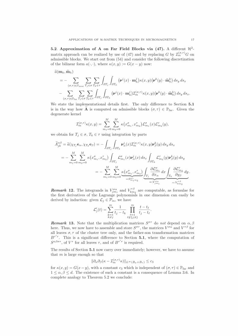
APPLICATIONS OF H-MATRIX TECHNIQUES IN MICROMAGNETICS 17
5.2. Approximation of A on Far Field Blocks via (47). A different H2-
matrix approach can be realized by use of (47) and by replacing G by I(σ,τ)m G on
admissible blocks. We start out from (54) and consider the following discretizationof the bilinear form a(·, ·), where κ(x, y) := G(x− y) now:
a(mh, mh)
= −∑
(σ,τ)∈Pnear
∑
Tj∈σ
∑
Tk∈τ
∫
∂Tj
∫
∂Tk
(νννj(x) ·mj
h
)κ(x, y)
(νννk(y) · mk
h
)dsy dsx
−∑
(σ,τ)∈Pfar
∑
Tj∈σ
∑
Tk∈τ
∫
∂Tj
∫
∂Tk
(νννj(x) ·mj
h
)I(σ,τ)m κ(x, y)
(νννk(y) · mk
h
)dsy dsx.
We state the implementational details first. The only difference to Section 5.1
is in the way how A is computed on admissible blocks (σ, τ) ∈ Pfar. Given thedegenerate kernel
I(σ,τ)m κ(x, y) =
M∑
m1=0
M∑
m2=0
κ(xσm1
, xτm2
)Lσm1
(x)Lτm2
(y),
we obtain for Tj ∈ σ, Tk ∈ τ using integration by parts
Aαβjk = a(χTj
eα, χTkeβ) = −
∫
∂Tj
∫
∂Tk
νννjα(x)I(σ,τ)m κ(x, y)νννkβ(y) dsy dsx
= −M∑
m1=0
M∑
m2=0
κ(xσm1
, xτm2
) ∫
∂Tj
Lσm1
(x)νννjα(x) dsx
∫
∂Tk
Lτm2
(y)νννkβ(y) dsy
= −M∑
m1=0
M∑
m2=0
κ(xσm1
, xτm2
)︸ ︷︷ ︸
=Sστm1m2
∫
Tj
∂Lσm1
∂xαdx
︸ ︷︷ ︸=:V σα
jm1
∫
Tk
∂Lτm2
∂yβdy
︸ ︷︷ ︸=:V τβ
km2
.
Remark 12. The integrands in V σαjm1
and V τβkm2
are computable, as formulae forthe first derivatives of the Lagrange polynomials in one dimension can easily bederived by induction: given Lj ∈ Pm, we have
L′j(t) =
m∑
k=1k 6=j
1
tj − tk
m∏
ℓ=1ℓ 6∈j,k
t− tℓtj − tℓ
.
Remark 13. Note that the multiplication matrices Sστ do not depend on α, βhere. Thus, we now have to assemble and store Sστ , the matrices V σα and V τβ forall leaves σ, τ of the cluster tree only, and the father-son transformation matricesBτ ′τ . This is a significant difference to Section 5.1, where the computation ofSαβστ , of V τ for all leaves τ , and of Bτ ′τ is required.
The results of Section 5.1 now carry over immediately; however, we have to assumethat m is large enough so that
‖∂α∂β(κ− I(σ,τ)m κ)‖L∞(Bσ×Bτ ) ≤ c3
for κ(x, y) = G(x− y), with a constant c3 which is independent of (σ, τ) ∈ Pfar and1 ≤ α, β ≤ d. The existence of such a constant is a consequence of Lemma 3.6. Incomplete analogy to Theorem 5.2 we conclude:
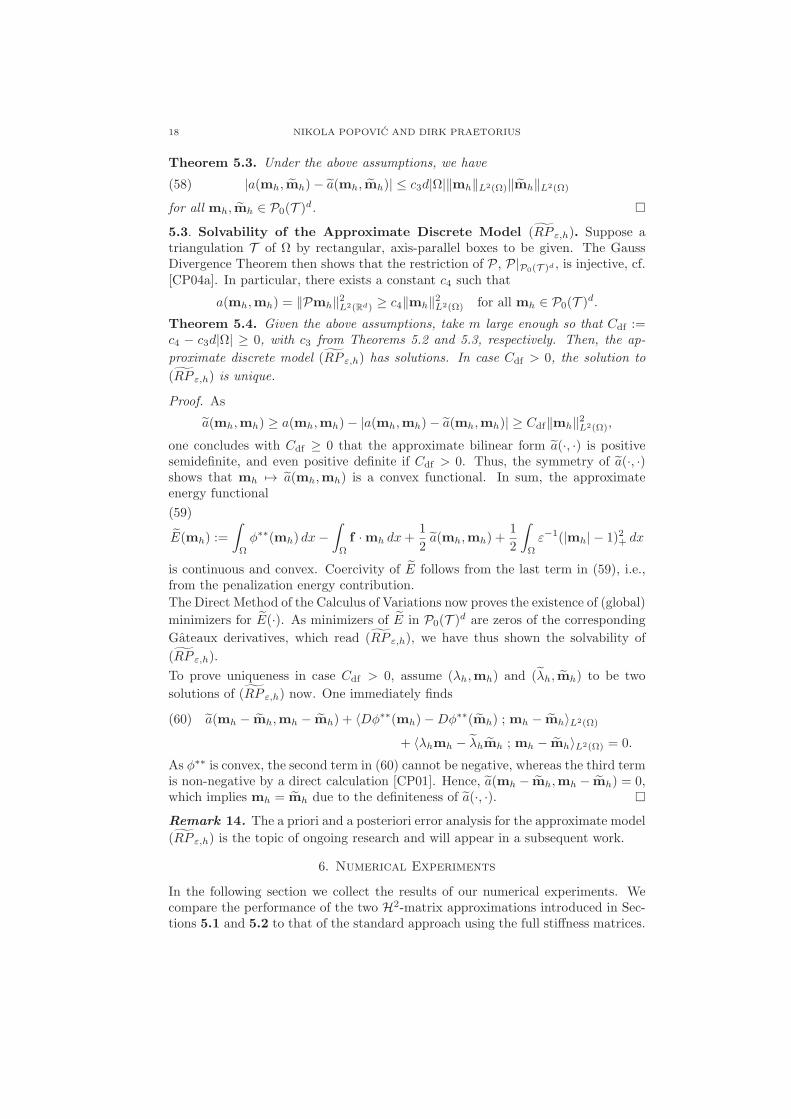
18 NIKOLA POPOVIC AND DIRK PRAETORIUS
Theorem 5.3. Under the above assumptions, we have
|a(mh, mh)− a(mh, mh)| ≤ c3d|Ω|‖mh‖L2(Ω)‖mh‖L2(Ω)(58)
for all mh, mh ∈ P0(T )d.
5.3. Solvability of the Approximate Discrete Model (RP ε,h). Suppose atriangulation T of Ω by rectangular, axis-parallel boxes to be given. The GaussDivergence Theorem then shows that the restriction of P, P|P0(T )d , is injective, cf.[CP04a]. In particular, there exists a constant c4 such that
a(mh,mh) = ‖Pmh‖2L2(Rd) ≥ c4‖mh‖2L2(Ω) for all mh ∈ P0(T )d.
Theorem 5.4. Given the above assumptions, take m large enough so that Cdf :=c4 − c3d|Ω| ≥ 0, with c3 from Theorems 5.2 and 5.3, respectively. Then, the ap-
proximate discrete model (RP ε,h) has solutions. In case Cdf > 0, the solution to
(RP ε,h) is unique.
Proof. As
a(mh,mh) ≥ a(mh,mh)− |a(mh,mh)− a(mh,mh)| ≥ Cdf‖mh‖2L2(Ω),
one concludes with Cdf ≥ 0 that the approximate bilinear form a(·, ·) is positivesemidefinite, and even positive definite if Cdf > 0. Thus, the symmetry of a(·, ·)shows that mh 7→ a(mh,mh) is a convex functional. In sum, the approximateenergy functional
E(mh) :=
∫
Ω
φ∗∗(mh) dx−∫
Ω
f ·mh dx+1
2a(mh,mh) +
1
2
∫
Ω
ε−1(|mh| − 1)2+ dx
(59)
is continuous and convex. Coercivity of E follows from the last term in (59), i.e.,from the penalization energy contribution.
The Direct Method of the Calculus of Variations now proves the existence of (global)
minimizers for E(·). As minimizers of E in P0(T )d are zeros of the corresponding
Gateaux derivatives, which read (RP ε,h), we have thus shown the solvability of
(RP ε,h).
To prove uniqueness in case Cdf > 0, assume (λh,mh) and (λh, mh) to be two
solutions of (RP ε,h) now. One immediately finds
(60) a(mh − mh,mh − mh) + 〈Dφ∗∗(mh)−Dφ∗∗(mh) ; mh − mh〉L2(Ω)
+ 〈λhmh − λhmh ; mh − mh〉L2(Ω) = 0.
As φ∗∗ is convex, the second term in (60) cannot be negative, whereas the third termis non-negative by a direct calculation [CP01]. Hence, a(mh − mh,mh − mh) = 0,which implies mh = mh due to the definiteness of a(·, ·).
Remark 14. The a priori and a posteriori error analysis for the approximate model
(RP ε,h) is the topic of ongoing research and will appear in a subsequent work.
6. Numerical Experiments
In the following section we collect the results of our numerical experiments. Wecompare the performance of the two H2-matrix approximations introduced in Sec-tions 5.1 and 5.2 to that of the standard approach using the full stiffness matrices.
APPLICATIONS OF H-MATRIX TECHNIQUES IN MICROMAGNETICS 19
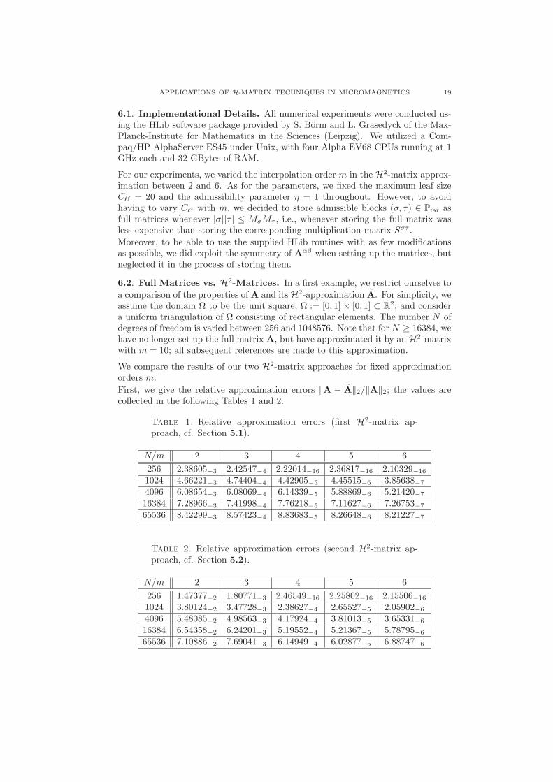
6.1. Implementational Details. All numerical experiments were conducted us-ing the HLib software package provided by S. Borm and L. Grasedyck of the Max-Planck-Institute for Mathematics in the Sciences (Leipzig). We utilized a Com-paq/HP AlphaServer ES45 under Unix, with four Alpha EV68 CPUs running at 1GHz each and 32 GBytes of RAM.
For our experiments, we varied the interpolation order m in the H2-matrix approx-imation between 2 and 6. As for the parameters, we fixed the maximum leaf sizeCℓf = 20 and the admissibility parameter η = 1 throughout. However, to avoidhaving to vary Cℓf with m, we decided to store admissible blocks (σ, τ) ∈ Pfar asfull matrices whenever |σ||τ | ≤ MσMτ , i.e., whenever storing the full matrix wasless expensive than storing the corresponding multiplication matrix Sστ .
Moreover, to be able to use the supplied HLib routines with as few modificationsas possible, we did exploit the symmetry of Aαβ when setting up the matrices, butneglected it in the process of storing them.
6.2. Full Matrices vs. H2-Matrices. In a first example, we restrict ourselves to
a comparison of the properties of A and its H2-approximation A. For simplicity, weassume the domain Ω to be the unit square, Ω := [0, 1]× [0, 1] ⊂ R
2, and considera uniform triangulation of Ω consisting of rectangular elements. The number N ofdegrees of freedom is varied between 256 and 1048576. Note that for N ≥ 16384, wehave no longer set up the full matrix A, but have approximated it by an H2-matrixwith m = 10; all subsequent references are made to this approximation.
We compare the results of our two H2-matrix approaches for fixed approximationorders m.
First, we give the relative approximation errors ‖A − A‖2/‖A‖2; the values arecollected in the following Tables 1 and 2.
Table 1. Relative approximation errors (first H2-matrix ap-proach, cf. Section 5.1).
N/m 2 3 4 5 6
256 2.38605−3 2.42547−4 2.22014−16 2.36817−16 2.10329−16
1024 4.66221−3 4.74404−4 4.42905−5 4.45515−6 3.85638−7
4096 6.08654−3 6.08069−4 6.14339−5 5.88869−6 5.21420−7
16384 7.28966−3 7.41998−4 7.76218−5 7.11627−6 7.26753−7
65536 8.42299−3 8.57423−4 8.83683−5 8.26648−6 8.21227−7
Table 2. Relative approximation errors (second H2-matrix ap-proach, cf. Section 5.2).
N/m 2 3 4 5 6
256 1.47377−2 1.80771−3 2.46549−16 2.25802−16 2.15506−16
1024 3.80124−2 3.47728−3 2.38627−4 2.65527−5 2.05902−6
4096 5.48085−2 4.98563−3 4.17924−4 3.81013−5 3.65331−6
16384 6.54358−2 6.24201−3 5.19552−4 5.21367−5 5.78795−6
65536 7.10886−2 7.69041−3 6.14949−4 6.02877−5 6.88747−6
20 NIKOLA POPOVIC AND DIRK PRAETORIUS
In summary, the errors in the second approach (cf. Section 5.2) seem to be largerby one order of magnitude. The convergence rates, however, are optimal in bothcases: every increase of m by one reduces the error by an order of magnitude. Notethat for N = 256 and m ≥ 4, our choice of Cℓf implies that there are no admissibleblocks; the error in this case is due to rounding. The error estimates themselvesare computed by a power iteration, with a maximum of 100 iterative steps.
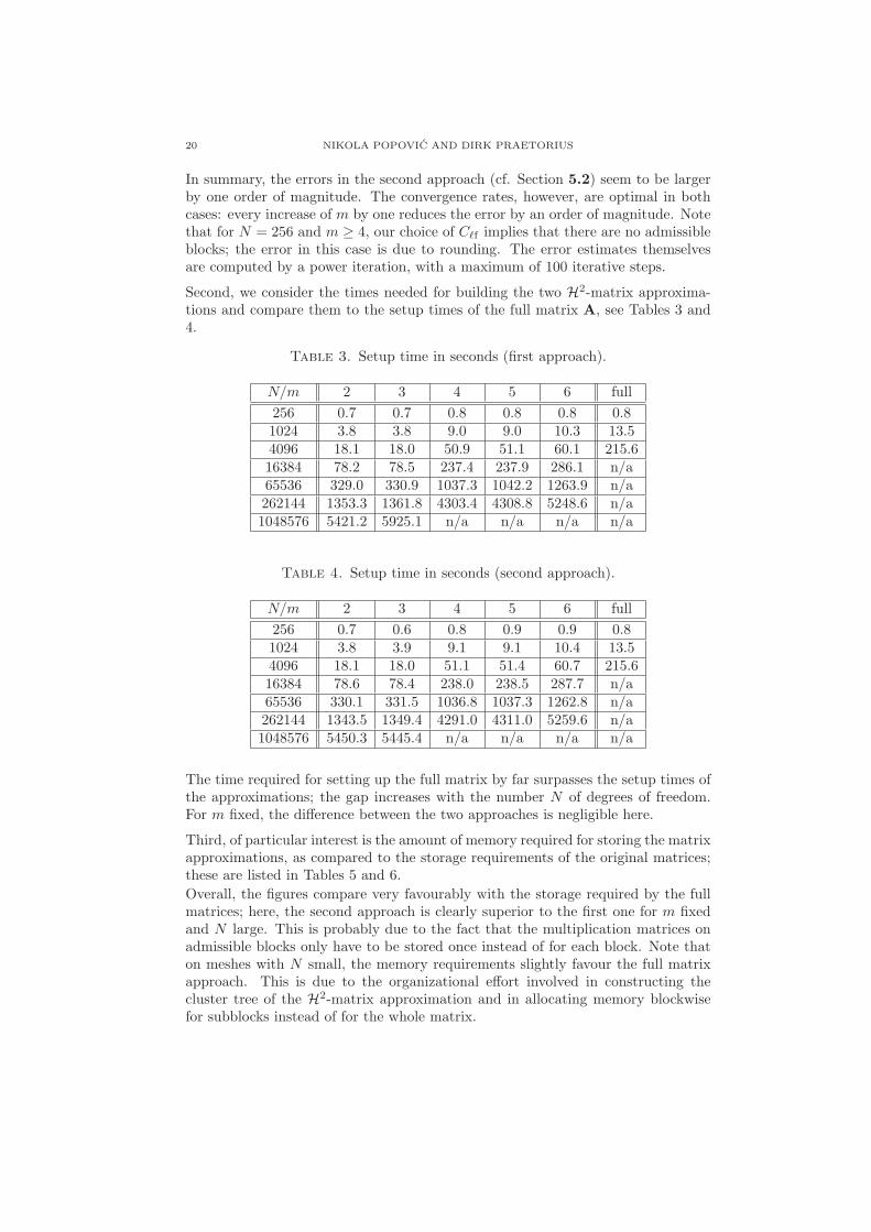
Second, we consider the times needed for building the two H2-matrix approxima-tions and compare them to the setup times of the full matrix A, see Tables 3 and4.
Table 3. Setup time in seconds (first approach).
N/m 2 3 4 5 6 full
256 0.7 0.7 0.8 0.8 0.8 0.81024 3.8 3.8 9.0 9.0 10.3 13.54096 18.1 18.0 50.9 51.1 60.1 215.616384 78.2 78.5 237.4 237.9 286.1 n/a65536 329.0 330.9 1037.3 1042.2 1263.9 n/a262144 1353.3 1361.8 4303.4 4308.8 5248.6 n/a1048576 5421.2 5925.1 n/a n/a n/a n/a
Table 4. Setup time in seconds (second approach).
N/m 2 3 4 5 6 full
256 0.7 0.6 0.8 0.9 0.9 0.81024 3.8 3.9 9.1 9.1 10.4 13.54096 18.1 18.0 51.1 51.4 60.7 215.616384 78.6 78.4 238.0 238.5 287.7 n/a65536 330.1 331.5 1036.8 1037.3 1262.8 n/a262144 1343.5 1349.4 4291.0 4311.0 5259.6 n/a1048576 5450.3 5445.4 n/a n/a n/a n/a
The time required for setting up the full matrix by far surpasses the setup times ofthe approximations; the gap increases with the number N of degrees of freedom.For m fixed, the difference between the two approaches is negligible here.
Third, of particular interest is the amount of memory required for storing the matrixapproximations, as compared to the storage requirements of the original matrices;these are listed in Tables 5 and 6.
Overall, the figures compare very favourably with the storage required by the fullmatrices; here, the second approach is clearly superior to the first one for m fixedand N large. This is probably due to the fact that the multiplication matrices onadmissible blocks only have to be stored once instead of for each block. Note thaton meshes with N small, the memory requirements slightly favour the full matrixapproach. This is due to the organizational effort involved in constructing thecluster tree of the H2-matrix approximation and in allocating memory blockwisefor subblocks instead of for the whole matrix.

APPLICATIONS OF H-MATRIX TECHNIQUES IN MICROMAGNETICS 21
Table 5. Memory requirement in KBytes/N (first approach).
N/m 2 3 4 5 6 full
256 5.2 5.6 6.8 7.2 7.6 6.01024 8.8 11.6 18.8 20.5 22.1 24.04096 11.4 16.2 28.9 34.6 42.6 96.016384 12.9 19.1 35.5 44.6 58.2 384.065536 13.7 20.7 39.3 50.6 67.9 1536.0262144 14.2 21.6 41.3 53.9 73.4 6144.01048576 14.4 22.1 n/a n/a n/a 24576.0
Table 6. Memory requirement in KBytes/N (second approach).
N/m 2 3 4 5 6 full
256 5.2 5.5 7.2 8.1 9.2 6.01024 8.3 9.4 18.6 19.9 22.5 24.04096 10.4 12.2 26.9 29.5 35.4 96.016384 11.6 13.8 31.8 35.6 44.1 384.065536 12.2 14.8 34.6 39.1 49.2 1536.0262144 12.6 15.2 36.0 40.9 51.9 6144.01048576 12.7 15.5 n/a n/a n/a 24576.0
Altogether, these numerical experiments underline the applicability of H-matrixtechniques to the discretized potential operator P from (RPε,h). For given approx-imation order m, the first approach leads to lesser approximation errors, but isotherwise also more costly numerically, as is reflected by the much higher storagerequirements.
In a certain sense, however, the two approaches seem almost equivalent: if werequire some fixed accuracy, the approximation order m always has to be higher byone in the second approach, as the errors lag behind by one order of magnitude.A comparison of the respective setup times and memory requirements then showsthe numerical cost to be almost even.
6.3. An Example with Known Exact Solution. In our second example, weconsider a model problem for the relaxed Landau-Lifshitz problem (RP ) taken from[CP04b]. As above, let the domain Ω be the unit square; assume Ω to be filled with
some uniaxial magnetized material, with the easy axis given by e = (−1, 1)/√2
and the corresponding normal by z = (1, 1)/√2, see Remark 1. Define (m, λ) ∈
W 1,∞(Ω;R2)× L∞(Ω) as
m(x) :=
x for |x| ≤ 1,
x/|x| for |x| > 1and λ(x) :=
0 for |x| ≤ 1,
1 for |x| > 1.(61)
Then, (m, λ) solves (RP ) with given right-hand side
f := Pm+ (m · z)z+ λm in L2(Ω;R2),(62)
cf. (11),(12). In the following, we replace Pm in (62) by PmT , where mT denotesthe piecewise integral mean of m. Note that there are no fully analytic examples
22 NIKOLA POPOVIC AND DIRK PRAETORIUS
for (RP ) with known solutions, which is why we have to restrict ourselves to thepresent model.
As m is Lipschitz continuous and therefore in W 1,∞(Ω;R2), the a priori analysisfrom [CP04b] yields ‖(m − mh) · z‖L2(Ω) = O(ε + h), with ε the penalizationparameter from (14). For our experiments, we choose ε = h and compute the
discrete solutionmh =∑2N
j=1 xjϕj with respect to the basis ϕ1, . . . , ϕ2N from (50)
by a classical Newton-Raphson scheme: the unknown coefficient vector x ∈ R2N is
determined as the unique zero of
F (x) :=(〈Pmh +Dφ∗∗(mh) + λhmh − f ; ϕj〉
)2Nj=1
= 0.(63)
[A detailed discussion on the relevance of ε can be found in [CP04b].] Note thatthe convergence of the Newton-Raphson method is not guaranteed mathematically,since F is only differentiable almost everywhere. The Jacobian of F can be written
as a finite sum DF (x) = A +∑N
j=1 Dj(x) with symmetric positive semidefinite
matricesDj(x) ∈ R2N×2N , cf. [CP04a]. For a triangulation by rectangular elements
such as ours, the matrix A can be shown to be positive definite by applying theGauss Divergence Theorem, see [CP04b]. We therefore employ a preconditionedconjugate gradient method, with the LU decomposition of a coarsened H-matrix
version of A as preconditioner.
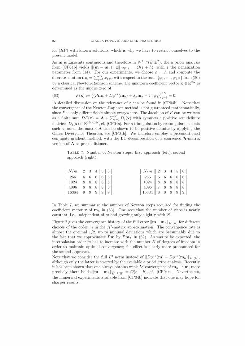
Table 7. Number of Newton steps: first approach (left), secondapproach (right).
N/m 2 3 4 5 6
256 6 6 6 6 61024 8 8 8 8 84096 8 8 8 8 816384 9 9 9 9 9
N/m 2 3 4 5 6
256 6 6 6 6 61024 8 8 8 8 84096 7 8 8 8 816384 8 8 9 9 9
In Table 7, we summarize the number of Newton steps required for finding thecoefficient vector x of mh in (63). One sees that the number of steps is nearlyconstant, i.e., independent of m and growing only slightly with N .
Figure 2 gives the convergence history of the full error ‖m−mh‖L2(Ω) for different
choices of the order m in the H2-matrix approximation. The convergence rate isalmost the optimal 1/2, up to minimal deviations which are presumably due tothe fact that we approximate Pm by PmT in (62). As was to be expected, theinterpolation order m has to increase with the number N of degrees of freedom inorder to maintain optimal convergence; the effect is clearly more pronounced forthe second approach.
Note that we consider the full L2 norm instead of ‖Dφ∗∗(m) − Dφ∗∗(mh)‖L2(Ω),although only the latter is covered by the available a priori error analysis. Recentlyit has been shown that one always obtains weak L2 convergence of mh m; moreprecisely, there holds ‖m − mh‖H−1(Ω) = O(ε + h), cf. [CP04c] . Nevertheless,
the numerical experiments available from [CP04b] indicate that one may hope forsharper results.

APPLICATIONS OF H-MATRIX TECHNIQUES IN MICROMAGNETICS 23
0.1
0.2
0.3
0.4
0.5
0.6
0.7
0.8
0.9
1
0
0.1
0.2
0.3
0.4
0.5
0.6
0.7
0.8
0.9
Figure 1. The discrete solution (mh, λh) of (RPε,h) as in themodel example for N = 1024, with mh on the left (displayed asvectors mh|T and |mh|T |) and λh on the right. In the white region,we have |mh| ≤ 1 and therefore λh = 0.
100
101
102
103
104
105
10−3
10−2
10−1
100
1
1/2
N
||m−
mh|| 2
m=2m=3m=4m=5m=6
100
101
102
103
104
105
10−3
10−2
10−1
100
1
1/2
N
||m−
mh|| 2
m=2m=3m=4m=5m=6
Figure 2. Experimental convergence of ‖m −mh‖L2(Ω) over N :first approach (left), second approach (right).
Acknowledgement. This work has been supported by the AustrianScience Fund FWF under grant P15274, “Reliable and Efficient Numer-ical Algorithms in Computational Micromagnetics”. The authors thankS. Borm and L. Grasedyck of the Max-Planck-Institute for Mathemat-ics in the Sciences (Leipzig) for providing them with the HLib software package, aswell as for several helpful comments.
References
[BG04] S. Borm and L. Grasedyck. Low-Rank Approximation of Integral Operators by Interpo-lation. Computing, 72:325–332, 2004.
[BGH03] S. Borm, L. Grasedyck, and W. Hackbusch. Introduction to Hierarchical Matrices withApplications. Eng. Anal. with B. Elem., 27:405–422, 2003.
[BH02] S. Borm and W. Hackbusch. H2-Matrix Approximation of Integral Operators by Inter-polation. Appl. Numer. Math., 43:129–143, 2002.
[BLM04] S. Borm, M. Lohndorf, and J.M. Melenk. Approximation of Integral Operators by
Variable-Order Interpolation. Numer. Math., 2004. To appear.

24 NIKOLA POPOVIC AND DIRK PRAETORIUS
[BS01] I. Babuska and T. Strouboulis. The Finite Element Method and its Reliability. NumericalMathematics and Scientific Computation. Oxford University Press, Inc., Oxford, 2001.
[CP01] C. Carstensen and A. Prohl. Numerical analysis of relaxed micromagnetics by penalisedfinite elements. Numer. Math., 90:65–99, 2001.
[CP04a] C. Carstensen and D. Praetorius. Effective Simulation of a Macroscopic Model for Sta-tionary Micromagnetics. Comput. Methods Appl. Mech. Engrg., 2004. To appear.
[CP04b] C. Carstensen and D. Praetorius. Numerical Analysis for a Macroscopic Model in Mi-cromagnetics. SIAM J. Numer. Anal., 2004. To appear.
[CP04c] C. Carstensen and D. Praetorius. Stabilization Yields Strong Convergence for a Macro-scopic Model in Micromagnetics. 2004. In preparation.
[DeS93] A. DeSimone. Energy Minimizers for Large Ferromagnetic Bodies. Arch. Rational Mech.
Anal., 125:99–143, 1993.[DL93] R.A. DeVore and G.G. Lorentz. Constructive Approximation, volume 303 of
Grundlehren der mathematischen Wissenschaften. Springer-Verlag, Berlin Heidelberg,1993.
[GH03] L. Grasedyck and W. Hackbusch. Construction and arithmetics of H-matrices. Comput-
ing, 70(4):295–334, 2003.
[Gie01] K. Giebermann. Multilevel Approximation of Boundary Integral Operators. Computing,67:183–207, 2001.
[Gra01] L. Grasedyck. Theorie und Anwendungen Hierarchischer Matrizen. PhD thesis,
Christian-Albrechts-Universitat, Kiel, 2001.[Hac02] W. Hackbusch. Direct Integration of the Newton Potential over Cubes Including a Pro-
gram Description. Computing, 68:193–216, 2002.[HKS00] W. Hackbusch, B. Khoromskij, and S.A. Sauter. On H2-matrices. In Lectures on Applied
Mathematics, pages 9–29. Springer-Verlag, Berlin Heidelberg, 2000.[HS98] A. Hubert and R. Schafer. Magnetic Domains: the Analysis of Magnetic Microstruc-
tures. Springer-Verlag, Berlin Heidelberg, 1998.[JK90] R.D. James and D. Kinderlehrer. Frustration in ferromagnetic materials. Cont. Mech.
Therm., 2:215–239, 1990.[KP01] M. Kruzık and A. Prohl. Young measure approximation in micromagnetics. Numer.
Math., 90(2):291–307, 2001.
[LM92] M. Luskin and L. Ma. Analysis of the finite element approximation of microstructure inmicromagnetics. SIAM J. Numer. Anal., 29(2):320–331, 1992.
[Ma91] L. Ma. Analysis and Computation for a Variational Problem in Micromagnetics. PhDthesis, University of Minnesota, Minneapolis, 1991.
[Mai99] M. Maischak. The Analytical Computation of the Galerkin Elements for the Laplace,Lame and Helmholtz Equation in 2D-BEM. Technical Report ifam48, Institut fur Ange-wandte Mathematik, Universitat Hannover, 1999.
[Mai00] M. Maischak. The Analytical Computation of the Galerkin Elements for the Laplace,Lame and Helmholtz Equation in 3D-BEM. Technical Report ifam50, Institut fur Ange-wandte Mathematik, Universitat Hannover, 2000.
[Ped97] P. Pedregal. Parametrized Measures and Variational Principles. Birkhauser, Basel,
1997.[Pra04] D. Praetorius. Analysis of the Operator −1div Arising in Magnetic Models. ZAA,
23:589–605, 2004.[Pro01] A. Prohl. Computational micromagnetism. Advances in Numerical Mathematics. B.G.
Teubner, Stuttgart, 2001.[Riv84] T.J. Rivlin. The Chebyshev Polynomials. Wiley Interscience, New York, 1984.[Tar95] L. Tartar. Beyond Young Measures. Meccanica, 30:505–526, 1995.
E-mail address: [email protected], [email protected]
Vienna University of Technology, Institute for Analysis and Scientific Computing,
Wiedner Hauptstraße 8-10, A-1040 Vienna, Austria