5C-02, page 15C-02, Version: August 3, 2000

Computational Micromagnetics: Prediction of time dependent and thermal properties

Thomas Schrefl, W. Scholz, Dieter Süss, J. FidlerInstitute of Applied and Technical Physics, Vienna University of Technology,

Wiedner Hauptstraße 8-10, A-1040 Vienna, Austria

ABSTRACT

Finite element modeling treats magnetization processes on a length scale of several nanometersand thus gives a quantitative correlation between the microstructure and the magnetic propertiesof ferromagnetic materials. This work presents a novel finite element / boundary element micro-magnetics solver that combines a wavelet-based matrix compression technique for magnetostaticfield calculations with a BDF / GMRES method for the time integration of the Gilbert equation ofmotion. In addition to the hysteresis properties, the numerical solution of the Gilbert equationsimulations show that metastable energy minima and nonuniform magnetic states within thegrains are important factors in the reversal dynamics at finite temperature.ation shows howreversed domains nucleate and expand. In an array of acicular NiFe elements the switching fieldvaries by about 8 kA/m depending on the magnetic state of neighboring elements. The switchingtime of submicron magnetic elements depends on the shape of the elements. Elements withslanted ends decrease the overall reversal time, as a transverse demagnetizing field suppressesoscillations of the magnetization. Thermal activated processes can be included adding a randomthermal field to the effective magnetic field. Thermally assisted reversal was studied forCoCrPtTa thin film media.

Keywords: Micromagnetism, Finite element method, Thermal activation

Corresponding Author:

Thomas SchreflInstitute of Applied and Technical PhysicsVienna University of TechnologyWiedner Hauptstr. 8-10/137A-1040 Vienna, Austria

phone: +43 1 58801 13729fax: +43 1 58801 13798email: thomas.schrefl@tuwien.ac.at

5C-02, page 2

1. Introduction

The development and application of modern magnetic materials requires a basic understanding ofthe magnetization processes that determine the magnetic properties. Micromagnetics relates themicroscopic distribution of the magnetization to the physical and chemical microstructure of amaterial. Recently, micromagnetic modeling has become an important tool to characterize themagnetic behavior of such different materials as thin film heads, recording media, patterned mag-netic elements, and nanocrystalline permanent magnets. In addition to magnetic imaging, compu-tational micromagnetics has become an important tool to investigate domain formation andmagnetization reversal [1]. The finite element method provides a general framework to calculatestatic, dynamic, and thermal properties of magnetic materials used as permanent magnets, sensorsor recording media. Micromagnetic finite element simulations are highly flexible, since it is pos-sible to incorporate the physical microstructure and to adjust the finite element mesh according tothe local magnetization [2].

The rapid progress of nanotechnology will lead to novel application of magnetic materials in spinelectronic devices, magnetic sensors, and functional materials within the next years [3]. A prereq-uisite for the application of structured magnetic materials is the detailed knowledge of the correla-tion between the physical and magnetic structure of the system. The design of smart materialsrequires to predict the response of the system to external fields and temperature as a function oftime. Magnetic sensors and magneto-mechanic devices consist of spatially distinct ferromagneticparts. Modeling their functional behavior requires to take into account the magnetostatic interac-tions between the magnetic elements. This work introduces a novel method for micromagneticsimulations that combines a hybrid finite element (FE) / boundary element (BE) method with awavelet matrix compression technique. Time integration schemes based on backward differencemethods proved to be efficient for the simulation of time dependent effects, since the micromag-netic equations are stiff. This method is applied to simulate the switching dynamics of magneticelements used in MRAM storage technology, where accurate prediction of the switching behavioris required. With increasing recording density and decreasing bit size, thermally activated magne-tization reversal becomes an important issue in magnetic recording [4]. This work combines afinite element model of the media with numerical methods for stochastic differential equations, inorder to solve the Langevin equation. The Langevin equation is believed to describe the randommotion of the magnetization at finite temperatures. The finite element method effectively treatsthe granular structure of thin film recording media. Variations in the size and shape of the grainsand the Cr segregation near grain boundaries can be taken into account. The magnetization withineach grain may become nonuniform, as each grain is further subdivided into tetrahedral finite ele-ments.

2. Micromagnetic and numerical background

Numerical micromagnetics starts from the total magnetic Gibbs free energy, Et, which is the sumof the exchange energy, the magneto-crystalline anisotropy energy, the magnetostatic energy, andthe Zeeman energy, and the magneto-elastic energy. The internal magnetostriction can beexpressed in the same mathematical form as the uniaxial or cubic magnetocrystalline anisotropy.Therefore, magneto-elastic effects may be ingored in the derivation of the governing equations.The total energy can be written as follows [5]:

5C-02, page 3

, (1)

where J = (β1,β2,β3)Js denotes the magnetic polarization. A is the exchange constant and fk is themagnetocrystalline anisotropy. Hd and Hext denote the demagnetizing and the external field,respectively. The minimization of Et provides an equilibrium distribution of the magnetic polar-ization. In order to resolve time dependent magnetization processes at finite temperatures, theLangevin equation [5]

(2)

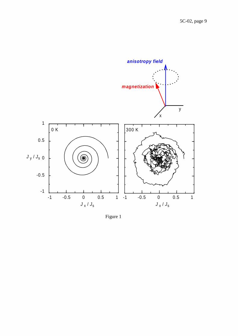
has to be solved. In order to treat thermally activated processes a stochastic, thermal field, Hth, isadded to the effective field, Heff. It accounts for the interaction of the magnetic polarization withthe microscopic degrees of freedom which causes the fluctuation of the magnetization distribu-tion. The effective field, Heff = – δEt/δJ, is the variational derivative of the magnetic Gibbs freeenergy. γ is the gyromagnetic ratio of the free electron spin, and α is the dimensionless Gilbertdamping constant. (2) gives the physical path of the system towards local energy minima. Thefirst term describes of the right hand side the gyromagnetic precession under the influence of ther-mal perturbation. The second term is a phenomenological damping term [6]. The damping termcauses the magnetization to become aligned parallel with the effective field. Thermal fluctuationscause the magnetization to from a random walk around its equilibrium position. If Hth is zero,equation (2) reduces to the Gilbert equation [6]. Fig. 1 compares the deterministic motion and thestochastic motion at 300K for a single magnetic moment. At the time t = 0, the angle between themagnetic moment and the magnetocrystalline anisotropy axes was set to 45°.

The effective field at the node k of an irregular finite element mesh may be approximatedusing the box scheme

, (3)

where Vk is the volume associated with the node k. The following conditions hold for the box vol-umes

for k ≠ l. (4)

The magnetic polarization is defined on the nodal point of the finite element mesh and is interpo-lated linearly within the each finite element.

The thermal field is assumed to be a Gaussian random process with the following statistical prop-erties:

, (5)

(6)

Et A βi∇ 2

i 1=

3

∑ fk J( ) 12---J Hd J Hext⋅–⋅–+ Vd∫=

J∂t∂

----- γ J– Heff Hth+( )× αJs

----J J∂t∂

-----×+=

Heffk( )

Heffk( ) 1

Vk

-----∂Et

∂J--------–=

Vkk

∑ Vd∫= Vk Vl∩, 0 =

Hth i,k( )⟨ ⟩ 0=

Hth i,k( )

Hth j,l( )⟨ ⟩ 2Dδijδklδ t t'–( )=

5C-02, page 4

The average of the thermal field vanishes taken over different realizations vanishes in each direc-tion i in space. The thermal field is uncorrelated in time and space. The strength of the thermalfluctuations follow from the fluctuation-dissipation theorem:

, (7)

where kB is the Boltzmann constant. The space discretization of (2) leads to a system of Langevintype equations with multiplicative noise.

At zero temperature the noise term vanishes and time integration can be performed using standardpackages [7] for stiff differential equations. Tsiantos and co-workers [8] showed that the micro-magnetic problem becomes considerably stiff in highly exchange coupled systems. In the stiffregime a combined BDF (backward difference formulae) / GMRES (generalized minimum resid-ual) method was found to be faster than explicit time integration schemes like the Adams methodor Runge-Kutta type methods. At finite temperature the noise term has to be taken into account.As shown by Garcia-Palacios and Lazaro [9] the equation has to be interpreted in the sense ofStratonovic, in order to obtain the correct thermal equilibrium properties. The numerical integra-tion of the stochastic differential equation is performed using the method of Heun. For the puredeterministic case the Heun method reduces to the standard second order Runge-Kutta method[10]. Numerical studies for simple spin systems confirmed that the Heun scheme is numericallymore stable and allows larger time steps than the Euler or the Milshtein scheme [11].

In order to speed up the calculation of the demagnetizing field Hd, we introduce a magnetic scalarpotential, U, which eliminates the long range terms from (1) [12]. A hybrid finite element /boundary integral method [13] is used for computing the magnetostatic boundary value problemfor U. This method is especially useful for the simulation of the magnetostatic interactions of dis-tinct magnetic elements, since no mesh is required outside the magnetic particles. We split thetotal magnetic scalar potential into U = U1 + U2. The potential U1 accounts for the divergence ofmagnetization within the particle and U2 is required to meet the boundary conditions. The latteralso carries the magnetostatic interactions between distinct magnetic particles. The potential U1 isthe solution of the Poisson equation with the natural boundary condition at the surface of the mag-netic particle. The potential U2 satisfies the Laplace equation everywhere and shows a jump at thesurface of the particle. The computation of U consists of three steps:

1. A standard finite element method is used to solve Poisson’s equation for U1.2. The potential U2 is calculated at the boundary

U2 = B U1 (8)

where B is a mxm matrix which relates the nodes at the surface to each other and U1 is the vec-tor of the U1 values at the surface nodes. The matrix B is dense and follows from the boundaryelement discretization of the double layer operator.

3. Once U2 at the boundary has been calculated, the values of U2 within the particles follow fromLaplace's equations with Dirichlet boundary conditions, which again can be a solved by stan-dard finite element technique.

Dk( ) αkBT

γJsVk

-------------=

5C-02, page 5

A discrete wavelet transform [14] is applied to transform the matrix B and U1. The matrix vectorproduct (8) can be evaluated in the wavelet bases. A sparse matrix is obtained after setting smallelements of the transformed matrix to zero. Only about 10% non-zero entries remain, which sig-nificantly reduces the storage requirements and computation time for the calculation of U2.

3. Magnetostatic interactions of magnetic nano-elements

Magnetic nano-elements may be the basic structural units of future patterned media or magneto-electronic devices [15]. Different magnetization reversal mechanisms occur depending on thestrength and direction of the magnetostatic interaction field. The simulations predict a spread inthe switching field due to magnetostatic interactions in the order of 8 kA/m for 200 nm wide,3500 nm long and 26 nm thick NiFe elements with a center-to-center spacing of 250 nm. Fig. 2gives the particle configuration used for the calculations. The original boundary element matrix ofthe system consists of 1.1 x 107 elements. After transformation and thresholding the matrix con-tains 1.9 x 106 non-zero entries, giving a sparsity of 83%. The demagnetization curve of the mid-dle element was calculated for a pair of switched or unswitched neighbors. The magnetization ofthe neighboring elements was fixed assuming a small uniaxial anisotropy parallel to the long axis.Fig. 3 compares the numerically calculated demagnetization curves obtained with the conven-tional boundary element method and with wavelet based matrix compression. In configuration A,the magnetostatic interaction field of the switched neighbors stabilizes the center element. In con-figuration B, the interaction field of the neighbors favors the reversal of the center element. Thecomparison shows that the wavelet based matrix compression method provides accurate results.Numerical studies showed [16] that the error owing to matrix compression is in the range from2 % to 5 %, for a sparsity between 80% a nd 90%. The numerical results agree well with experi-mental data obtained from Lorentz microscopy [17].

4. Switching dynamics of submicron elements

Koch and coworkers [18] investigated the switching behavior of micron-sized magnetic thin filmsexperimentally and numerically. They observed switching times less then 500 ps. In this work, theinfluence of the geometric shape on the reversal dynamics was investigated. Submicron NiFe ele-ments with an extension of 200x100x10 nm3 switch well below 1 ns for an applied field of 80 kA/m, assuming a Gilbert damping constant of 0.1. The elements reverse by nonuniform rotation.Under the influence of an applied field, the magnetization starts to rotate near the ends, followedby the reversal of the center. This process only requires about 0.1 ns. In what follows, the magne-tization component parallel to the field direction shows oscillations which decay within a time of0.4 ns. The excitation of spin waves originates from the gyromagnetic precession of the magneti-zation around the local effective field. A much faster decay of the oscillations occurs in elementswith slanted ends, where surface charges cause in transverse magnetostatic field. Fig. 4 whichcompares the time evolution of the magnetization for NiFe elements with rounded and slantedends clearly shows the effect of the element symmetry on magnetization reversal. To further ana-lyze this ringing phenomena Fig. 5 gives the Zeeman energy, the exchange energy, and the mag-netostatic energy as a function of time. The plots show that an energy transfer occurs frommagnetostatic energy to the exchange and Zeeman energy and vice versa. During the initial rota-tion of the magnetization, magnetic surface charges at the edges drastically increase the magneto-static energy. In what follows, a nonuniform state which reduces the magnetostatic energy isformed. The magnetization changes periodically between a highly nonuniform magnetic stateswith low magnetostatic but high exchange energy and a magnetic state with high magnetostatic

5C-02, page 6

energy. In addition, Fig. 5 presents a snapshot of the magnetization configuration during this pro-cess.

5. Thermal processes in thin film media

Finite element based micromagnetics is applied to study thermally assisted switching of thin filmmedia in the high speed regime. Fig. 6 shows the finite element model of the grain structure. Themagnetization within each grain may become nonuniform, as each grain is further subdivided intotetrahedral finite elements. The film thickness is 20 nm. The magnetocrystalline anisotropy axesare randomly oriented in-plane. The width of the Cr-enriched region near the grain boundaries isabout 2 nm. In addition, Fig. 6 gives the demagnetization curves obtained from deterministic cal-culations. The step at an external field of Hext = – 250 kA/m indicates a metastable magnetizationconfiguration which has to be passed during magnetization reversal.

In the numerical experiments the following procedure was applied. First the sample was saturatedunder the influence of an applied field of three times the anisotropy field. Then the field wasreduced to zero and the remanent state was calculated. Both calculations where performedneglecting thermal fluctuations. The resulting magnetization configuration was used as initialstate to calculate the thermal equilibrium state at 300 K for zero applied field using Langevindynamics. Then a reversed field was instantaneously applied to the thermal equilibrium state, inorder to simulate magnetization reversal at finite temperatures. The intrinsic magnetic properties(Js = 0.43 T, Ku = 2.2 x 105 J/m3) where taken from [19]. The exchange constants where adjustedto A = 10-11 J/m and A* = 0.6x10-11 J/m, in order to obtain a coercive field of about 255 kA/m at300 K. A and A* denote the intragrain and intergrain exchange constants, respectively. The simu-lations of magnetization reversal were repeated several times, taking into account the stochasticnature of the process. The magnetization switches in less than 1 ns in about 80% of the calcula-tions. However, reversal times up to 20 ns and higher are observed for about 20% of the realiza-tions. Fig. 7 which gives the probability of not switching shows that the fraction of systems whichremain unswitched after 1 ns decreases with increasing reversed field. The applied field is about70% of the deterministic coercive field.

The system switches from the high remanent state to a meta-stable state where it may remaintrapped for several nanoseconds. Fig. 8 gives the magnetization distribution in the remanent state,r, and in the metastable state, m. In the metastable state the bottom left grain has changed its mag-netization direction. For further visualization of the stochastic reversal process, we plot the differ-ence between the current magnetic state and the remanent state, r, as illustrated in Fig. 8. The greyscale maps the difference between the remanent state, r, and the meta-stable state, m. Fig. 9 com-pares the time evolution of the magnetization patterns for two different realizations of the stochas-tic process. The system either switches rapidly, forming a channel of reversed magnetization (A).Or the magnetization oscillates around the metastable state (B). After the partial reversal of thecenter grain, the system turns back to a state close to the original metastable state. This process isrepeated several times, as the oscillations are triggered by thermal fluctuations. Eventually thesystem may escape from the metastable state, leading to a complete reversal. The results clearlyshow that metastable energy minima and nonuniform magnetic states within the grains are impor-tant factors in the reversal dynamics at finite temperature.

5C-02, page 7

6. Summary

The results of micromagnetic finite element calculations enable the visualization of complexmagnetization phenomena. Thus modeling provides a better understanding of fast switchingdynamics at finite temperatures. The application of state of the art numerical techniques for thesolution of the partial differential equations considerably reduces computation time.

Acknowledgements

This work was supported by the Austrian Science Fund (Y-132 PHY). The authors thank V. Tsi-antos, U. Nowak, and D. Hinzke for helpful discussions and J. Chapman and K. Kirk for provid-ing experimental data.

References

[1] E. D. Dahlberg and J. G. Zhu, Physics Today 48 (1995) 34.[2] T. Schrefl, J. Magn. Magn. Mater. 207 (1999) 45.[3] M. Johnson, IEEE Spectrum, February 2000, 33.[4] D. Weller and A. Moser, IEEE Trans. Magn. 35 (1999) 4423.[5] W. F. Brown Jr., Micromagnetics, Wiley, New York, 1963.[6] T. L. Gilbert, Phys. Rev. 100 (1955) 1243.[7] A. C. Hindmarsh, L. R. Petzold, Computers in Physics 9 (1995) 148.[8] V. D. Tsiantos, J. J. Miles, and B. K. Middleton, in Proc. 3rd European Conference on

Numerical Mathematics and Advanced Applications, Enumath 99 (World Scientific).[9] L. Garcia-Palacios and F. J. Lazaro, Phys. Rev. B 58 (1998) 14937.[10]P. E. Kloeden and E. Platen, Numerical Solution of Stochastic Differential Equations. Berlin,

Heidelberg: Springer, 1995.[11]W. Scholz, Diploma Thesis, Vienna University of Technology, 1999.[12]P. Asselin and A. A. Thiele, IEEE Trans. Magn. 22 (1986) 1876.[13]D. R. Fredkin, T. R. Koehler, IEEE Trans. Magn. 26 (1990) 415.[14]W. H. Press, S. A. Teukolsky, W. T. Vetterling, B. P. Flannery, Numerical recipes in Fortran

77: The art of scientific computing, Cambridge University Press, 1992.[15]S. Y. Chou, Proceedings of the IEEE 85 (1997) 652.[16]T. Schrefl, D. Suss, J. Fidler, Proceedings of the MSM 2000, San Diego, March 2000.[17]K. J. Kirk, J. N. Chapman and C. D. W. Wilkinson, J. Appl. Phys. Lett. 71 (1997) 539.[18]R. H. Koch, J. G. Deak, D. W. Abraham, P. L. Trouilloud, R. A. Altman, Y. Lu, W. J. Gal-

lagher, R. E. Scheuerlein, K. P. Roche, and S. S. P. Parkin, Physical Review Letters 81 (1998)4512.

[19]E. N. Abarra I. Okamoto T. Suzuki, J. Appl. Phys. 85 (1999) 5015.

5C-02, page 8

Figure captions

Fig. 1. Path of the magnetization vector towards equilibrium for a small Co sphere. Gyromagneticprecession dominates the motion for a damping parameter of α = 0.01. Left: Deterministicmotion neglecting thermal fluctions; right: Random walk at 300 K.

Fig. 2. Array of NiFe nanoelements for the simulation of magnetostatic inteactions, using theboundary element method (solid line) and wavelet based matrix compression (dashed line).

Fig. 3. Numerically calculated demagnetization curves of the center element for a pair ofswitched (A) and unswichted (B) neighbors. Solid lines: conventional boundary element method,dashed line: wavelet based matrix compression.

Fig. 4. Time evolution of the magnetization for a NiFe element with an extension of200 x 100 x 10 nm3. The Gilbert damping constant used in the calculations was 0.1.

Fig. 5. Micromagnetic energy contributions as a function of time the reversal of the element withrounded end. The dotted, dashed and long-dashed line give the magnetostatic, exchange, and Zee-man energy, respectively. The inset shows the magnetization distribution after 0.18ns.

Fig. 6. Left: Model of a CoCrPtTa thin film medium for the investigation of thermally activatedreversal processes. Right: Demagnetization curve obtaind from solving Gilbert equation.

Fig. 7. Probability of not switching of the model system for different reversed fields.

Fig. 8. Plots of the difference from the remanent state provide a means to visualize magnetizationreversal.

Fig. 9. Magnetization patterns as a function of time for two different realizations of the stochasticreversal process under the influence of a field of Hext = – 255 kA/m.

5C-02, page 9

Figure 1

-1 -0.5 0 0.5 1M x

-1

-0.5

0

0.5

1

My

-1 -0.5 0 0.5 1M x

-1

-0.5

0

0.5

1

My

0 K 300 K

-1 -0.5 0 0.5 1J x / Js

-1 -0.5 0 0.5 1J x / Js

-1

-0.5

0

0.5

1

J y / Js

xy

anisotropy field

magnetization

5C-02, page 10

Figure 2

Figure 3

A B

A B

5C-02, page 11

Figure 4

0 0.1 0.2 0.3 0.4 0.5 0.6time (ns)

−1

−0.5

0

0.5

1

J/J s

rounded endsslanted ends

rounded ends

slanted ends

5C-02, page 12

Figure 5

Figure 6

magnetostatic

exchange

Zeeman

-500 -250 0 250

Hext (kA/m)

0

0.2

0.4

0.6

0.8

J/J s

m

500

r

10 nm

5C-02, page 13

Figure 7

0.1 1.0

tim e (ns)

0

0.2

0.4

0.6

0.8

1

prob

abili

ty o

f not

sw

itchi

ng

0 .3

255 kA/m

260 kA /m265 kA/m

5C-02, page 14

Figure 8

remanent state m etastable state

Hext

difference = |r – m |

5C-02, page 15

Figure 9

0.004 ns

0.012 ns

0.015 ns

0.02 ns

Hext = 255 kA/mA Btim

e