introduction - konicaminolta.com.cn · 3-3: lcd measurement differences for ca-210 lcd flicker...
TRANSCRIPT
Introduction
This document provides information regarding color measurement in general and the color measurement of display devices using the CA-210/CA-210Plus in particular. It is divided into 6 major sections:
• The information in this document is subject to change without notice.
1: Measurement Principle:
This section introduces color measurement and color-measuring instruments, and also discusses the technical advantages of the CA-210/CA-210Plus as well as measurement items for specific display types. 2: Definitions of Accuracy Standards and Repeatability:
This section discusses the standards used for determining accuracy and repeatability of the CA-210/CA-210Plus, and the traceability system. 3: Measurement Results
This section shows actual measurement results obtained using the CA-210/CA-210Plus, and discusses differences in measurement results obtained with the different instruments. 4: CA-SDK Software Explanation
This section explains how to use the CA-SDK to control the CA-210/CA-210Plus with your own software.
5: Application Examples
This section describes examples of actual systems using the CA-210/CA-210Plus.
6: Related Standards
This section describes some display-related international standards and how the CA-210/CA-210Plus relate to these standards.
1

Copyrights/Trademarks
Copyright Notice:
© Copyright 2007 KONICA MINOLTA SENSING INC.
All rights reserved.
Trademarks: • Windows, Visual Basic, and Visual C++ are trademarks or registered trademarks of Microsoft Corp.
• Company names and product names mentioned in this document are trademarks or registered trademarks of their respective companies.
Notice Regarding Component Names: • In this document, the component names continue to be listed as "Minolta" in some cases.
2

Table of Contents
Introduction ..............................................................................................................1
Copyrights/Trademarks ...........................................................................................2
1: Measurement Principle ........................................................................................7
1: Measurement Principle ........................................................................................7 1-1: Chromaticity and Color Measurement.......................................................................................7
1-1-1: Chromaticity.....................................................................................................................7 1-1-2: Measuring Color ..............................................................................................................8
1-2: About Color-Measuring Instruments .........................................................................................9 1-2: About Color-Measuring Instruments ...................................................................................9 1-2-1: Tristimulus Colorimeters ................................................................................................10 1-2-2: Spectroradiometers .......................................................................................................11 1-2-3: Absolute-Value Error for Tristimulus Colorimeters ........................................................12 1-2-4: Calibration of Tristimulus Colorimeters..........................................................................13 1-2-5: User Calibration of Tristimulus Colorimeters.................................................................16 1-2-6: Inter-Instrument Error for Tristimulus Colorimeters .......................................................18 1-2-7: Tristimulus Colorimeters vs. Spectroradiometers..........................................................19
1-3: Analyzer Mode.........................................................................................................................22 1-3-1: Overview of Analyzer Mode...........................................................................................22 1-3-2: Analyzer Mode Principle: Explanation of Overview (Details) ........................................23 1-3-3: Analyzer Mode Principle: Explanation of Calculations (Details)....................................25
1-4: Matrix Calibration ....................................................................................................................26 1-4-1: Matrix Calibration Overview...........................................................................................26 1-4-2: Concept of Matrix Calibration ........................................................................................27 1-4-3: Matrix Calibration Process 1: RGB Calibration (Detailed Explanation).........................30 1-4-4: Matrix Calibration Process 2: WRGB Calibration (Detailed Explanation) .....................32
1-5: Optical System Features .........................................................................................................34 1-5-1: Optical System Features ...............................................................................................34 1-5-2: Optical System and Measurement Advantages ............................................................35
1-5-2-1: Low-Luminance Measurement ............................................................................35 1-5-2-2: Narrow Viewing Angle/Uniform Viewing Angle....................................................36 1-5-2-3: Reduced Influence of Luminance/Chromaticity Variation....................................37
1-6: Circuit Features .......................................................................................................................38 1-6-1: Differences between CA-210 A/D Conversion and Conventional Methods ..................38 1-6-2: Advantages of Successive A/D method ........................................................................39
1-6-2-1: Measurement of even lower luminance levels.....................................................39 1-6-2-2: Reduced measurement time................................................................................39 1-6-2-3: Flicker measurement ...........................................................................................39
1-7: LCD Flicker Measurement.......................................................................................................40 1-7-1: What is LCD Flicker? .....................................................................................................40
1-7-1-1: How Flicker Occurs..............................................................................................40 1-7-1-2: LCD Drive Systems and Images Likely to Cause Flicker ....................................41 1-7-1-3: Flicker Measurement Examples ..........................................................................42
1-7-2: Flicker Measurement Methods ......................................................................................43 1-7-2-1: Flicker Measurement ...........................................................................................43 1-7-2-2: Explanation of Flicker Measurements by Contrast Method.................................44
1-7-2-2-1: Overview of Flicker Measurement by Contrast Method ..........................................44 1-7-2-2-2: Data Processing for Contrast Method (Details).......................................................45 1-7-2-2-3: Differences from the VESA Standard Contrast Method (Details) ............................47
1-7-2-3: Explanation of Flicker Measurements by JEITA Method.....................................49 1-7-2-3-1: Overview of Flicker Measurement by JEITA Method ..............................................49 1-7-2-3-2: Data Processing for JEITA Method (Details)...........................................................50 1-7-2-3-2-1: Differences from Contrast Method .......................................................................54 1-7-2-3-3: CA-210 Data Processing for JEITA Method (Details) .............................................55
3

1-7-2-3-3-1: Equation Used by CA-210 for JEITA Method.......................................................56 1-7-2-3-3-2: Explanation of JEITA Method Equation ...............................................................57 1-7-2-3-3-3: Additional Information Regarding JEITA Equation...............................................58 1-7-2-3-3-4: Differences from the VESA Standard ..................................................................59
1-8: PDP (Plasma Display Panel) Measurements (CA-100Plus/CA-210 Universal Probe)...........60 1-8-1: What is a PDP? .............................................................................................................60 1-8-2: Relation to Chromatic Luminance Meter .......................................................................63
2: Definitions of Accuracy Standards and Repeatability ....................................65 2-1: Definition of Luminance/Chromaticity Accuracy Standards and Repeatability .......................65
2-1-1: Accuracy ........................................................................................................................66 2-1-1-1: Definition of Accuracy ..........................................................................................66 2-1-1-2: Luminance Range for Certified Accuracy ............................................................67 2-1-1-3: Light Sources for Certified Accuracy (Details) .....................................................68
2-1-2: Repeatability ..................................................................................................................70 2-1-2-1: Definition of Repeatability ....................................................................................70 2-1-2-2: Light Sources for Certified Repeatability (Details)...............................................71
2-1-3: Measurement Accuracy.................................................................................................72 2-1-3-1: What is Measurement Accuracy? ........................................................................72
2-1-4: Traceability ....................................................................................................................73 2-2: Definition of Flicker Accuracy Standards and Repeatability ...................................................75
2-2-1: Accuracy ........................................................................................................................76 2-2-1-1: Definition of Accuracy (Flicker) ............................................................................76 2-2-1-2: Basic Concept......................................................................................................77 2-2-1-3: Main Body Section ...............................................................................................78 2-2-1-4: Probe Section ......................................................................................................79 2-2-1-5: CA-210 System Accuracy....................................................................................80
2-2-2: Repeatability ..................................................................................................................81 2-2-2-1: Definition of Repeatability (Flicker) ......................................................................81
2-2-3: Measurement Accuracy.................................................................................................82 2-2-3-1: What is Measurement Accuracy? ........................................................................82
3: Measurement Results ........................................................................................83 3-1: LCD Measurement Differences for CA-210, CA-110, and CS-1000.......................................83
3-1-1: Measurement of White: High Luminance (Details)........................................................83 3-1-2: Measurement of White: Low Luminance .......................................................................86 3-1-3: Measurement of Primary Colors....................................................................................88 3-1-4: Measurement of Intermediate Colors ............................................................................89
3-2: Gamma Characteristics Comparison ......................................................................................91 3-2-1: Comparison of Gamma Characteristics Measurements................................................91
3-3: LCD Measurement Differences for CA-210 LCD Flicker Measuring Probes and CS-1000....95 3-3-1: Measurements of White.................................................................................................95 3-3-2: Measurements of Primary Colors ..................................................................................96
3-4: Flicker Measurement Accuracy ...............................................................................................97 3-4-1: Flicker Measurement Accuracy: Contrast Method ........................................................97 3-4-2: Flicker Measurement Accuracy: JEITA Method ............................................................99
3-5: Measurement Speed ............................................................................................................ 102 3-5: Measurement Speed (Detailed Explanation) ................................................................. 102
3-6: CRT Measurement Differences for CA-100 and CA-100Plus.............................................. 104 3-6-1: Measurements of White.............................................................................................. 104 3-6-2: Measurements of Primary Colors ............................................................................... 105
3-7: CA-100Plus and CA-100 Measurement Error for CRTs and PDPs..................................... 108 3-7-1: Measurement of White at High Luminance (CRT) ..................................................... 108 3-7-2: Measurement of White at Low Luminance (CRT) ...................................................... 109 3-7-3: Measurement of White on PDP (Plasma Display Panel) ........................................... 110 3-7-4: Repeatability Comparison .......................................................................................... 111
4: CA-SDK Software Explanation ........................................................................112 4-1: What is COM? ...................................................................................................................... 112
4-1: Introduction .................................................................................................................... 112
4

4-1-1: COM Interface ............................................................................................................ 113 4-1-1-1: Interface ............................................................................................................ 113 4-1-1-2: COM Interface................................................................................................... 114 4-1-1-3: COM Interface Programming............................................................................ 116
4-1-2: Automation.................................................................................................................. 118 4-1-3: Regarding COM.......................................................................................................... 119
4-2: Creating a VC++ application using the CA-SDK.................................................................. 121 4-2: Creating a VC++ application using the CA-SDK ........................................................... 121 4-2-1: Creating the SDK Application ..................................................................................... 122
4-2-1-1: Creating the Application Project ....................................................................... 122 4-2-1-2: Creating the UI (User Interface)........................................................................ 123 4-2-1-3: Adding Code for the UI Objects ........................................................................ 124 4-2-1-4: CA-SDK Programming...................................................................................... 125
4-2-1-4-1: CA-SDK Object Creation ......................................................................................125 4-2-1-4-2: Using the CA-SDK Objects ...................................................................................129 4-2-1-4-3: Creating the Sink Object .......................................................................................132 4-2-1-4-4: Sink Object Creation/Connection and Event Handling..........................................136 4-2-1-4-5: Error Handling.......................................................................................................139 4-2-1-4-6: Const.h File...........................................................................................................140
4-2-2: Creating the SDK Application (Detailed Explanations)............................................... 142 4-2-2: Creating the SDK Application (Detailed Explanations) ........................................ 142 4-2-2-1: Creating the Application Project ....................................................................... 143 4-2-2-2: Creating the UI (User Interface)........................................................................ 148 4-2-2-3: Adding Code for the UI Objects ........................................................................ 150 4-2-2-4: CA-SDK Programming...................................................................................... 153
4-2-2-4-1: CA-SDK Object Creation ......................................................................................153 4-2-2-4-2: Using the CA-SDK Objects ...................................................................................155 4-2-2-4-3: Creating the Sink Object .......................................................................................156 4-2-2-4-4: Sink Object Creation/Connection and Event Handling..........................................159 4-2-2-4-5: Const.h File...........................................................................................................160
4-3: CA-SDK Sample Software Control Methods........................................................................ 162 4-3: CA-SDK Sample Software Control Methods ................................................................. 162 4-3-1: CaControl (for Performing Settings on CA-Series Instruments)................................. 163
4-3-1-1: CaControl Properties/Methods ......................................................................... 164 4-3-1-2: CaControl: Using in VB..................................................................................... 166 4-3-1-3: CaControl: Using in VC++ (MFC) ..................................................................... 169
4-3-2: xyControl (for Displaying Data in xy Color Space) ..................................................... 174 4-3-2: xyControl (for Displaying Data in xy Color Space)............................................... 174 4-3-2-1: xyControl Properties/Methods .......................................................................... 175 4-3-2-2: xyControl: Using in VB...................................................................................... 178 4-3-2-3: xyControl: Using in VC++ (MFC) ...................................................................... 180
4-4: CA-SDK VB Sample Software.............................................................................................. 182 4-4-1: Color/Flicker Measurement ........................................................................................ 183 4-4-2: Gamma Measurement ................................................................................................ 187 4-4-3: Contrast Measurement ............................................................................................... 188 4-4-4: Calibration................................................................................................................... 189
4-5: Creating a Visual Basic .NET Application using the CA-SDK.............................................. 194 4-5-1: Creating the VB.NET project ...................................................................................... 195 4-5-2: Setting references to CA_SDK................................................................................... 197 4-5-3: Creation of Application GUI/Code .............................................................................. 200
5: Application Examples ......................................................................................207 5-1: CA-210 Application Example (White Balance Adjustment System)..................................... 207
5-1-1: White Balance Adjustment ......................................................................................... 207 5-1-2: System Block Diagram (White Balance Adjustment) ................................................. 209 5-1-3: White Balance Adjustment Software Functions ......................................................... 210 5-1-4: White Balance Adjustment Time ................................................................................ 211 5-1-5: GUI (White Balance Adjustment)................................................................................ 212
5-2: CA-210 Application Example (Gamma Adjustment System) ............................................... 214 5-2-1: Gamma Adjustment .................................................................................................... 214 5-2-2: System Block Diagram (Gamma Adjustment) ............................................................ 215
5

5-2-3: Gamma Adjustment Process...................................................................................... 216 5-2-4: Gamma Adjustment Time........................................................................................... 218 5-2-5: GUI (Gamma Adjustment) .......................................................................................... 219
6: Related Standards............................................................................................220 6-1: CA-210 and ED-2522 Standards.......................................................................................... 220
6-1-1: Introduction ................................................................................................................. 220 6-1-2: Measurement Items.................................................................................................... 221 6-1-3: Measurement Items and CA-210................................................................................ 222 6-1-4: Brief Definitions of Measurement Items...................................................................... 224
6-2: CA-210 and VESA Standards .............................................................................................. 226 6-2-1: Introduction ................................................................................................................. 226 6-2-2: Measurement Conditions and CA-210 ....................................................................... 227 6-2-3: Measurement Items and CA-210................................................................................ 230 6-2-4: Brief Definitions of Measurement Items...................................................................... 233
6-3: sRGB.................................................................................................................................... 239 6-3: What is sRGB? .............................................................................................................. 239
Index ..........242
6

1: Measurement Principle 1-1: Chromaticity and Color Measurement
1-1-1: Chromaticity
A variety of color systems have been devised in order to express color quantitatively. The simplest of these color systems is the RGB system. The RGB system is a system which attempts to express all colors as ratios of the three colors R, G, and B. The CIE (Commission Internationale de l′Éclairage) defined three monochromatic lights as primary stimuli: R was defined as light with a wavelength of 700.0nm, G as light with a wavelength of 546.1nm, and B as light with a wavelength of 435.8nm. However, it was found that expressing certain colors using this system required negative values in the mixture ratio, which was a problem. In order to solve this problem and make all values in the mixture ratio positive, the CIE selected new primary stimuli. This is the XYZ system defined by the CIE in 1931, and is currently the most widely used color system. The x, y chromaticity diagram for this color system is shown in Figure 1-1-1.
However, one problem with this color system is that color differences (the difference between two colors, which on the chromaticity diagram would be the distance between the two color points) on the chromaticity diagram do not correspond well to the degree of color perceived by human observers. For example, if we take the x, y values on the chromaticity diagram for a color in the region when only green is displayed on an LCD, and the x, y values for a color in the region where only blue is displayed, and change the values by the same amounts, the human observer would perceive the blue color as having been changed more than the green color. A system which solves this problem is the u′v′ system. In the u′v′ system, the difference between two colors separated by the same distance in any region on the chromaticity diagram will be perceived by a human observer as approximately the same amount of color difference. Because of this advantage, there is a recent trend to use this color system more frequently. The chromaticity diagram for this color system is shown in Figure 1-1-2.
7

1-1-2: Measuring Color
In order to measure color in the XYZ system, it is necessary to obtain the XYZ outputs from sensors with spectral sensitivities equal to the x, y, z color-matching functions shown in Figure 1-1-3.
These outputs are then used in the following equations to calculate chromaticity x, y:
For the u'v' system, chromaticity u',v' is determined from X, Y, and Z using the following equations:
8

1-2: About Color-Measuring Instruments
1-2: About Color-Measuring Instruments
Color-measuring instruments can be broadly classified according to their measuring method into two types: tristimulus colorimeters and spectroradiometers. This section will explain the measurement principle and characteristic features of the two types.
9

1-2-1: Tristimulus Colorimeters
Tristimulus colorimeters (more properly called "direct-reading tristimulus colorimeters") use three sensors having the spectral sensitivities of the color-matching functions defined by the CIE in 1931. The outputs from these sensors are used to determine the chromaticity and luminance of the subject. Figure 1-2-1 shows an example of the spectral sensitivity of the sensors. These sensors are typically comprised of a photocell and optical filters. If the spectral intensity of the subject light source is S(λ) and the spectral sensitivities of the 3 sensors are x′(λ), y′(λ), and z′(λ) respectively, then the respective outputs X, Y, and Z of the sensors would be
where
λ: Wavelength (Wavelength range: Visible range)
The chromaticity x,y and luminance Lv can then be obtained from the output values using the following equations:
10

1-2-2: Spectroradiometers
A spectroradiometer first measures the intensity emitted by the subject light source at each wavelength. These intensity values are then multiplied by the corresponding wavelength of the color-matching functions defined by the CIE in 1931 to obtain the chromaticity x, y and the luminance Lv.
The typical structure of this measuring instrument is shown in the figure below. The light from the subject light source is collected by the instrument′s objective lens, and passes through a spectral device, where it is separated by wavelength. The wavelength-separated light is then projected onto a line sensor, and the intensity at each wavelength is obtained from the output of each element of the line sensor.
If the emitted spectral intensity at each wavelength is S′(λ) and the color-matching functions are x(λ), y(λ), and z(λ) respectively, then
where
λ: Wavelength (Wavelength range: Visible range)
Thereafter, the calculations for determining chromaticity x, y and luminance Lv are the same as for tristimulus colorimeters.
11
1-2-3: Absolute-Value Error for Tristimulus Colorimeters
In this section, we will explain the reason for errors in the absolute measured values for tristimulus colorimeters.
In general, the spectral sensitivity of tristimulus colorimeters is determined by the combination of the spectral transmittance of the optical filters and the spectral sensitivity of the sensors.
If the resulting spectral sensitivity exactly matches the CIE 1931 color-matching functions, there would be no differences in the absolute-value chromaticity determined by tristimulus colorimeters regardless of the light source used. However, with current filter technology, we cannot make the spectral sensitivity of tristimulus colorimeters exactly match the CIE color-matching functions, as shown in Figure 1-2-1. These differences from the CIE color-matching functions result in some errors when taking absolute measurements.
The mechanism of this phenomenon is as follows:
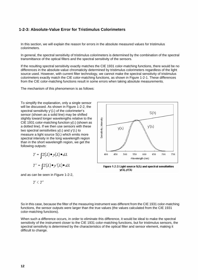
To simplify the explanation, only a single sensor will be discussed. As shown in Figure 1-2-2, the spectral sensitivity y′(λ) of the colorimeter′s sensor (shown as a solid line) may be shifted slightly toward longer wavelengths relative to the CIE 1931 color-matching function y(λ) (shown as a dotted line). If we then use sensors with these two spectral sensitivities y(λ) and y′(λ) to measure a light source S(λ) which emits more spectral intensity in the long wavelength region than in the short wavelength region, we get the following outputs:
and as can be seen in Figure 1-2-2,
So in this case, because the filter of the measuring instrument was different from the CIE 1931 color-matching functions, the sensor outputs were larger than the true values (the values calculated from the CIE 1931 color-matching functions).
When such a difference occurs, in order to eliminate this difference, it would be ideal to make the spectral sensitivity of the instrument closer to the CIE 1931 color-matching functions, but for tristimulus sensors, the spectral sensitivity is determined by the characteristics of the optical filter and sensor element, making it difficult to change.
12

1-2-4: Calibration of Tristimulus Colorimeters
In order to compensate for the problem described in the previous section, a method in which the sensor outputs are multiplied by appropriate coefficients to make the results the same as the true values is used. This is called "Calibration".
Specifically, the coefficient ky is calculated as
and thereafter ky•Y′ is used to calculate chromaticity. For these calculations, the Y value is obtained using a spectroradiometer or other measuring instrument with a spectral sensitivity which is the same as (or extremely close to) the CIE 1931 color-matching functions.
The results obtained in this way are shown in Figure 1-2-3.
In this diagram, the sensor spectral sensitivity y′′(λ) (shown as a solid line) is:
and the spectral sensitivity is reduced by a constant ratio, so that the resulting sensor output Y′′ is equivalent to Y. The equations would be as follows:
In the same way, kx and kz are calculated for X and Z, and these coefficients are used in the chromaticity calculations so that true measurement values can be obtained.
13
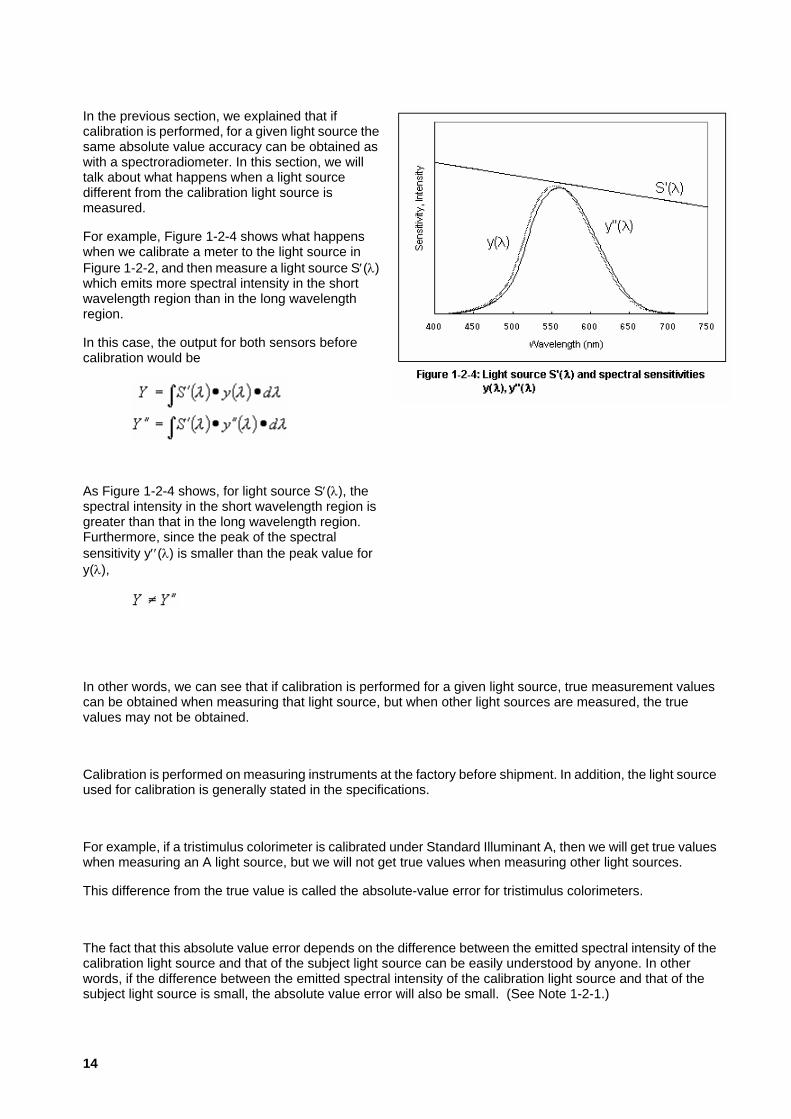
In the previous section, we explained that if calibration is performed, for a given light source the same absolute value accuracy can be obtained as with a spectroradiometer. In this section, we will talk about what happens when a light source different from the calibration light source is measured.
For example, Figure 1-2-4 shows what happens when we calibrate a meter to the light source in Figure 1-2-2, and then measure a light source S′(λ) which emits more spectral intensity in the short wavelength region than in the long wavelength region.
In this case, the output for both sensors before calibration would be
As Figure 1-2-4 shows, for light source S′(λ), the spectral intensity in the short wavelength region is greater than that in the long wavelength region. Furthermore, since the peak of the spectral sensitivity y′′(λ) is smaller than the peak value for y(λ),
In other words, we can see that if calibration is performed for a given light source, true measurement values can be obtained when measuring that light source, but when other light sources are measured, the true values may not be obtained.
Calibration is performed on measuring instruments at the factory before shipment. In addition, the light source used for calibration is generally stated in the specifications.
For example, if a tristimulus colorimeter is calibrated under Standard Illuminant A, then we will get true values when measuring an A light source, but we will not get true values when measuring other light sources.
This difference from the true value is called the absolute-value error for tristimulus colorimeters.
The fact that this absolute value error depends on the difference between the emitted spectral intensity of the calibration light source and that of the subject light source can be easily understood by anyone. In other words, if the difference between the emitted spectral intensity of the calibration light source and that of the subject light source is small, the absolute value error will also be small. (See Note 1-2-1.)
14
Notes
Note 1-2-1:
For CA series, the CA-210 uses an LCD as the calibration light source, and the CA-100 Plus uses a CRT. Even though there are differences in the phosphors used by CRTs, there is a tendency for the differences in spectral intensity to be small. The same trend is seen with LCDs.
15

1-2-5: User Calibration of Tristimulus Colorimeters
As stated in the previous section, calibration is performed at the factory before shipment.
However, in addition to this calibration (factory shipment calibration), the user of the measuring instrument can also select a light source and perform calibration. Such calibration is referred to as "user calibration".
As explained above, calibration is only effective when measuring the same kind of light source as the calibration light source. The same can be said of user calibration. In this section, we will discuss points that need to be considered regarding user calibration.
Figure 1-2-5 shows the case in which the spectral sensitivity y′(λ) (shown as a solid line) of the measuring instrument′s sensor is shifted toward the long wavelength region compared to the CIE 1931 color-matching functions y(λ) (shown as a dotted line). In addition, the emitted spectral intensity S′′(λ) of the factory calibration light source is shown; it is uniform over the entire wavelength range from the short wavelength region to the long wavelength region.
In this case, the peak of the sensor′s spectral sensitivity y′(λ) is equal to the peak of the color-matching function y(λ).
In other words, at the time of shipment from the factory, the spectral sensitivity of the sensor is y′(λ) as shown in Figure 1-2-5.
If this instrument is then used to measure the light source S(λ) used in Figure 1-2-2, which has greater spectral intensity in the long wavelength region than in the short wavelength region, absolute value error would occur, as was clearly seen in Figure 1-2-2.
User calibration is performed to eliminate this absolute value error.
User calibration is performed in the same way as factory shipment calibration, in that the sensor outputs are multiplied by appropriate coefficients so that the values obtained are the same as the true values.
Therefore, if user calibration was performed using the light source S(λ) in Figure 1-2-2, the spectral sensitivity of the sensor would be the same as y′′(λ) in Figure 1-2-3.
But if we then used this spectral sensitivity to measure the light source S′(λ) in Figure 1-2-4, which has higher emitted spectral intensity in the short wavelength region than in the long wavelength region, absolute value error would occur, as was explained previously.
However, if light source S′(λ) was measured using a sensor with a peak spectral sensitivity equal to that of the color-matching function y(λ), the sensor output value would be smaller than the true value. Because of this, if user calibration was performed using light source S(λ), the sensor output would be even smaller, making the difference from the true value larger.
• It can be seen that the absolute value error which occurs when light source S′(λ) is measured with an instrument which has been user calibrated to light source S(λ) is much larger compared to the error which occurs when the same light source is measured using a factory-calibrated instrument.
16
• If light source S′(λ) is measured with an instrument which has been user calibrated to light source S′(λ), true values can be obtained. In other words, even when using tristimulus colorimeters, true values can be obtained if user calibration is performed for each light source to be measured.
In general, tristimulus colorimeters have memory to store multiple user-calibration values, and by using this memory function, true values can be obtained for the various light sources. (See Note 1-2-2.) Effective use of this memory function enables tristimulus colorimeters to be high-accuracy measuring instruments.
Notes
Note 1-2-2:
For example, the CA-210 and CA-100 Plus provide 99 memory channels for user calibration.
17

1-2-6: Inter-Instrument Error for Tristimulus Colorimeters
"Inter-instrument error" is the difference in measured values when two instruments measure the same light source. It is said to be a problem for tristimulus colorimeters.
With current technology, it is difficult to eliminate variations in the spectral transmittance of the optical filters used in each instrument, which is then seen as the inter-instrument error for the measuring instruments. This will be explained below.
If we look at two tristimulus colorimeters, their respective spectral responses are as shown in Figure 1-2-3 (when factory-calibrated to light source S(λ), the sensor outputs for light source S(λ) are the same).
If we then measure light source S′(λ) from Figure 1-2-4, the sensor outputs from the two units are different. This difference between the two outputs is what results in inter-instrument error.
The user calibration function can be used to reduce this inter-instrument error.
To be specific, when using two measuring instruments to, for example, measure light source A, first use one of the instruments to measure the light source and record the measured values. Then, measure the same light source A with the second instrument, and perform user calibration so that the measured values are the same as the values recorded for the first instrument.
If the above procedure is performed, measurements of light source A can be taken with no inter-instrument error.
18

1-2-7: Tristimulus Colorimeters vs. Spectroradiometers
In this section, the characteristic features of the optical systems of tristimulus colorimeters and spectroradiometers will be described, and then the advantages/disadvantages of the two systems will be discussed.
Simplified diagrams of the optical systems are shown in Figures 1-2-6a (tristimulus colorimeter) and 1-2-6b (spectroradiometer).
The tristimulus colorimeter uses a structure in which the objective lens converges the light from the subject light source onto the sensor section. Methods in which the converged light is then transmitted via optical fibers to each sensor in order to improve the photoefficiency are also used.
In a spectroradiometer, the light from the subject light source converged by the objective lens is projected by a second lens onto a diffraction grating. The incident light is diffracted by the diffraction grating and reflected onto another converging lens, which projects the diffracted light onto a line sensor. The energy at each wavelength can then be obtained from the output of the corresponding sensor element.
From the above, it can be seen that the optical system of a spectroradiometer is more complicated than that of a tristimulus colorimeter.
19

Next, let′s look at a table of the advantages and disadvantages of each system.
Table 1: Comparison of tristimulus colorimeter and spectroradiometer
Tristimulus colorimeter
Spectro-radiometer
Reason
Absolute value accuracy
Low High Spectroradiometers use the color-matching functions directly for calculations.
The spectral response of tristimulus colorimeters is different from the color-matching functions. (See Note 1-2-3.)
Measurement speed
Fast Slow Tristimulus colorimeters use only 3 sensors. Spectroradiometers use up to several hundred sensors, so the amount of data to be processed is greater.
Sensitivity High Low Tristimulus colorimeters use only 3 sensors, but spectroradiometers use up to several hundred sensors, so the amount of light per sensor is much smaller for spectroradiometers than for tristimulus colorimeters
Size Small sensor section
Large sensor section
As shown in Figures 1-2-6a and 1-2-6b, the optical system of tristimulus colorimeters is comprised of a subjective lens and a sensor, but for a spectroradiometer, many optical components are necessary, including 3 lenses and the sensor plus a diffraction grating. In addition, a certain amount of space is necessary for imaging by each of the lenses.
Price Low High As shown in Figures 1-2-6a and 1-2-6b, spectroradiometers use many components in their optical system, and in addition some of these components are expensive.
Influenced by polarization?
No Yes Tristimulus colorimeters do not use any optical components which are influenced by polarization, but in spectroradiometers, the diffraction grating is influenced by polarization
When measuring a light source, it is necessary to grasp the features of each system and use the appropriate instrument (direct-reading tristimulus colorimeter or spectroradiometer) for the application.
(See Note 1-2-4.)
Notes
Note 1-2-3:
A spectroradiometer measures the spectral energy at each wavelength directly, and it then uses the color-matching functions directly in its calculations. For this reason, its spectral response (how it converts the measured energy into luminance and chromaticity) can be said to be exactly equal to the
20

color-matching functions. Also because of this, it can take high-accuracy measurements without having to recalibrate it for each different light source.
Note 1-2-4:
For tristimulus colorimeters, the Chroma Meter CS-100A (Konica Minolta), BM-7 (Topcon) and BM-5A (Topcon) using a photomultiplier tube are well known.
For spectroradiometers, the Spectroradiometer CS-1000A (Konica Minolta), SR-3 (Topcon), and PR-704 (Photo Research) are well known.
Topcon is a trademark of Topcon Corp.
Photo Research is a trademark of Photo Research Co., Ltd.
21

1-3: Analyzer Mode
1-3-1: Overview of Analyzer Mode
Analyzer mode is a measurement mode used for high-speed adjustment of the white balance of displays on the production line.
White-balance adjustment would be simple if, for example, adjusting G caused only the y to change. If this was the case, it would be easy to just adjust G for the deficiency or excess of y.
However, in actuality, adjusting G changes not only the y, but also the x. This is because the spectral emission range for G includes portions not only in the y(λ) color-matching function region, but also in the x(λ) function region, as shown in Figure 1-3-1.
For example, if only the y is shifted in relation to the target color, even if G is adjusted so that the chromaticity value y matches the desired value, the x is also shifted, and thus becomes different than the x of the target. Further, if R is then adjusted to make the x match the target value, y is also shifted away from the target value.
Adjustment in such a situation can be performed if a person could remember how much x and y change as G is adjusted, and performing adjustment accordingly. However, there would be problems with such a method, because it requires a lot of skill, and in addition, since the ratios would be different for different types of displays, it would be necessary to remember the characteristics of each type of display.
Analyzer mode is a function which was designed to solve the problems stated above. By using this mode, R/G/B intensities can be obtained directly instead of xy values, making white-balance adjustment easier to perform.
22
1-3-2: Analyzer Mode Principle: Explanation of Overview (Details)
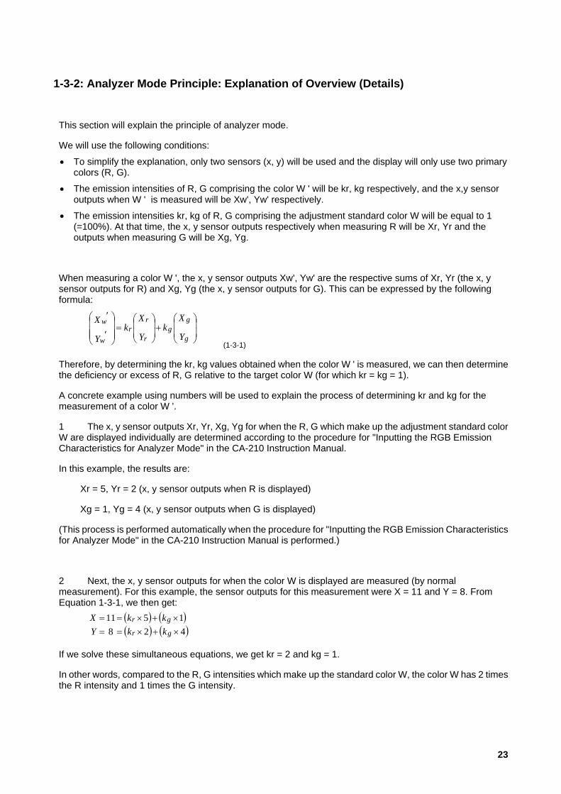
This section will explain the principle of analyzer mode.
We will use the following conditions:
• To simplify the explanation, only two sensors (x, y) will be used and the display will only use two primary colors (R, G).
• The emission intensities of R, G comprising the color W ' will be kr, kg respectively, and the x,y sensor outputs when W ' is measured will be Xw', Yw' respectively.
• The emission intensities kr, kg of R, G comprising the adjustment standard color W will be equal to 1 (=100%). At that time, the x, y sensor outputs respectively when measuring R will be Xr, Yr and the outputs when measuring G will be Xg, Yg.
When measuring a color W ', the x, y sensor outputs Xw', Yw' are the respective sums of Xr, Yr (the x, y sensor outputs for R) and Xg, Yg (the x, y sensor outputs for G). This can be expressed by the following formula:
⎟⎟
⎠
⎞
⎜⎜
⎝
⎛+
⎟⎟
⎠
⎞
⎜⎜
⎝
⎛=
⎟⎟⎟
⎠
⎞
⎜⎜⎜
⎝
⎛
′
′
g
gg
r
rr
w
w
Y
Xk
Y
Xk
Y
X
(1-3-1)
Therefore, by determining the kr, kg values obtained when the color W ' is measured, we can then determine the deficiency or excess of R, G relative to the target color W (for which kr = kg = 1).
A concrete example using numbers will be used to explain the process of determining kr and kg for the measurement of a color W '.
1 The x, y sensor outputs Xr, Yr, Xg, Yg for when the R, G which make up the adjustment standard color W are displayed individually are determined according to the procedure for "Inputting the RGB Emission Characteristics for Analyzer Mode" in the CA-210 Instruction Manual.
In this example, the results are:
Xr = 5, Yr = 2 (x, y sensor outputs when R is displayed)
Xg = 1, Yg = 4 (x, y sensor outputs when G is displayed)
(This process is performed automatically when the procedure for "Inputting the RGB Emission Characteristics for Analyzer Mode" in the CA-210 Instruction Manual is performed.)
2 Next, the x, y sensor outputs for when the color W is displayed are measured (by normal measurement). For this example, the sensor outputs for this measurement were X = 11 and Y = 8. From Equation 1-3-1, we then get:
( ) ( )( ) ( )428
1511×+×==×+×==
gr
gr
kkYkkX
If we solve these simultaneous equations, we get kr = 2 and kg = 1.
In other words, compared to the R, G intensities which make up the standard color W, the color W has 2 times the R intensity and 1 times the G intensity.
23

This will be explained further using vector diagrams.
The relationship between the standard color W, its components R, G, and the x, y sensor outputs can be expressed graphically as shown in Figure 1-3-2.
On the XY graph, the vectors R and G are drawn to represent the measurement results for each individual color which makes up W, and the total vector W.
The relationship shown in Figure 1-3-2 is determined by the operation performed in Step 1 above.
Next, we draw the vector W ' in Figure 1-3-3 using the results of the measurement of W ' performed in Step 2 above (X = 11, Y = 8).
We can then see from Figure 1-3-3 that the W ' vector is the sum of 2 times R plus G.
Therefore, if we consider that
( ) ( )GVector RVector Vector W' ×+×= gr kk
then kr = 2 and kg = 1
Steps 1 and 2 above are the process for determining kr and kg using the relationships shown in Figures 1-3-2 and 1-3-3.
24

1-3-3: Analyzer Mode Principle: Explanation of Calculations (Details)
The situation where 3 sensors x, y, z are used and the display has 3 primary colors R, G, B will now be explained using equations.
The variables used in the equations are defined as:
• kr, kg, kb are the respective emission intensities for R, G, B which comprise the color W '. Xw', Yw', Zw' are the respective x, y, z sensor outputs when the color W ' is measured.
• The emission intensities kr, kg, kb for the R, G, B respectively which comprise the adjustment standard color W will all be equal to 1 (= 100%). At that time, the x, y, z sensor outputs respectively when measuring R will be Xr, Yr, Zr; the outputs when measuring G will be Xg, Yg, Zg; and the outputs when measuring B will be Xb, Yb, Zb.
The x, y, z sensor outputs Xw', Yw', Zw' obtained when measuring the color W ' are the respective sums of the x, y, z sensors when R, G, and B are measured individually. This can be expressed as:
⎟⎟⎟⎟
⎠
⎞
⎜⎜⎜⎜
⎝
⎛
⎟⎟⎟⎟
⎠
⎞
⎜⎜⎜⎜
⎝
⎛
=
⎟⎟⎟⎟
⎠
⎞
⎜⎜⎜⎜
⎝
⎛
+
⎟⎟⎟⎟
⎠
⎞
⎜⎜⎜⎜
⎝
⎛
+
⎟⎟⎟⎟
⎠
⎞
⎜⎜⎜⎜
⎝
⎛
=
⎟⎟⎟⎟⎟
⎠
⎞
⎜⎜⎜⎜⎜
⎝
⎛
′
′
′
b
g
r
bgr
bgr
bgr
b
b
b
b
g
g
g
g
r
r
r
r
w
w
w
k
k
k
ZZZ
YYY
XXX
Z
Y
X
k
Z
Y
X
k
Z
Y
X
k
Z
Y
X
(1-3-2)
Therefore, the respective intensity ratios kr, kg, kb relative to the R, G, B which comprise the adjustment standard color W can be calculated from the equation:
⎟⎟⎟⎟⎟
⎠
⎞
⎜⎜⎜⎜⎜
⎝
⎛
′
′
′
⎟⎟⎟⎟
⎠
⎞
⎜⎜⎜⎜
⎝
⎛
=
⎟⎟⎟⎟
⎠
⎞
⎜⎜⎜⎜
⎝
⎛−
w
w
w
bgr
bgr
bgr
b
g
r
Z
Y
X
ZZZ
YYY
XXX
k
k
k 1
(1-3-3)
In this way, by obtaining the values of kr, kg, kb when the color W ' is measured, the deficiency or excess of R, G, B for a standard color W (kr = kg = kb = 1) can be determined.
25

1-4: Matrix Calibration
1-4-1: Matrix Calibration Overview
Conventional calibration (referred to here as single-point white calibration) of tristimulus colorimeters means making the measured value for a specific color for a specific light source match the known value for that color.
However, when this single-point white calibration is used, even for the same light source (display), if the calibration values for a certain color are used and a different color is measured on the same CRT, there may be some error in the measurement value. In particular, when the calibration values for white are used and a primary color (R, G, or B) is measured, the measurement error becomes large. (See section 1-2-3: Absolute-Value Error for Tristimulus Colorimeters.)
Matrix calibration is a calibration method which is suitable for displays which create images using RGB additive compound colors. (See Note 1-4-1.). With matrix calibration, calibration is performed simultaneously for 4 colors (R, G, B, and W) instead of for only a single color. By using this method, measurement values with low error can be obtained over a wide color range for a given display.
Notes
Note 1-4-1:
The mixing of two or more primary colors.
Here, for a display which uses the primary colors R, G, and B to create a color image, the color is referred to as an "additive primary color" if the XYZ values for the color (for a given white, for example) are the sum of the XYZ values for the R, G, and B primary colors which comprise the color.
26

1-4-2: Concept of Matrix Calibration
This section will explain matrix calibration using diagrams.
Single-point white calibration
Let's consider the case of a display for which the relationship between the measured values and true values (desired values) is as shown in Figure 1-4-1a. In this example, for a certain white point, the measured value is at the position indicated by and the true value is indicated by ×. As shown in the figure, the measured value has an error in the negative x direction and the positive y direction relative to the true value. In addition, the region of colors which can be reproduced on the display is the region enclosed by the solid line when the measured values are used, but is the region enclosed by the dotted line when the true values are used.
Single-point white calibration makes the measured point ( mark) match the true value (× mark). As a result, the reproduceable color region for measured values (the solid-outline triangular region) is shifted, and the relationship between the measured values and true values becomes as shown in Figure 1-4-1b. As a result, as can be seen in the figure, although the measured value and true value match for the single white point. the measurement error between measured values and true values for other colors remains. In the case shown in the figure, the measurement error for the primary color R has increased.
27

Matrix calibration
The relationships between measured values and true values before and after matrix calibration are shown in Figures 1-4-2a and 1-4-2b respectively.
With matrix calibration, the measurement values for primary colors are also made to match the true values. In other words, if there are differences between the measured values and true values of the primary colors as shown in Figure 1-4-2a, linear transformations are performed on the measured values in the direction of the arrows in the diagram so that the measured values match the true values (Figure 1-4-2b).
In other words, matrix calibration is performed to determine the linear coefficients.
Table 1 shows the measurement errors calculated by simulation when white points at various color temperatures and the primary colors RGB are displayed on a certain LCD and measured with a tristimulus colorimeter which has been calibrated by single-point white calibration (calibration point: 6500K white) and matrix calibration.
∆ x ∆ y ∆ x ∆ yWhite (6500K) 0.0000 0.0000 0.0000 0.0000White (5000K) 0.0017 0.0017 0.0000 0.0000
White (13000K) 0.0020 0.0018 0.0000 0.0000R 0.0282 0.0241 0.0000 0.0000G 0.0399 0.0231 0.0000 0.0000B 0.0128 0.0081 0.0000 0.0000
Table 1: Results of num erical s im ulation of absolute -value error for each calibration m ethod
Single-point w hite calibration Matrix calibration
From this table, it can be seen that theoretically, for the LCD used for calibration, matrix calibration resulted in no measurement error for all colors. However, with single-point white calibration, although there was no measurement error for the 6500K white calibration point, there were large measurement errors for the primary colors. (See Note 1-4-2.)
28

Notes
Note 1-4-2:
The numerical simulation was performed under the condition that the color was an additive compound color.
Further, the chromaticity errors were calculated from the sensor outputs obtained using the equations:
( ) ( )( ) ( )( ) ( ) λλλ
λλλλλλ
∆••=∆••=∆••=
∑∑∑
zSZySYxSX
where
x(λ), y(λ), z(λ): Spectral response of a tristimulus colorimeter measured using a spectrophotometer
S(λ): Emitted spectral intensity of a marketed LCD measured using a spectrophotometer.
29

1-4-3: Matrix Calibration Process 1: RGB Calibration (Detailed Explanation)
First, the calibration data x, y, Lv for the R, G, B calibration points (referred to as the standard R, G, B points) are input (in other words, the matrix calibration values are input). The X, Y, Z count values can then be calculated from these x, y, Lv values. The X, Y, Z count values calculated for each standard point R, G, and B will be Xr' Yr' Zr', Xg' Yg' Zg', and Xb' Yb' Zb' respectively.
According to the principle of analyzer mode (see sections 1-3-1: Overview of Analyzer Mode and 1-3-2: Analyzer Mode Principle: Explanation of Overview (Details)) for a given color W', the RGB intensities kr, kg, kb (ratio of standard colors R, G, and B) can be calculated.
Since the Xw' Yw' Zw' values used for determining the chromaticity of the color W' are the sums of the X Y Z counts for the R G B which comprise the color W', they can be expressed using the following equation:
⎟⎟⎟⎟⎟
⎠
⎞
⎜⎜⎜⎜⎜
⎝
⎛
′
′
′
+
⎟⎟⎟⎟⎟
⎠
⎞
⎜⎜⎜⎜⎜
⎝
⎛
′
′
′
+
⎟⎟⎟⎟⎟
⎠
⎞
⎜⎜⎜⎜⎜
⎝
⎛
′
′
′
=
⎟⎟⎟⎟⎟
⎠
⎞
⎜⎜⎜⎜⎜
⎝
⎛
′
′
′
b
b
b
g
g
g
r
r
r
w
w
w
Z
Y
X
kb
Z
Y
X
kg
Z
Y
X
kr
Z
Y
X
(1-4-1)
So if the values kr, kg, kb have been determined using the R, G, B calibration values, the X, Y, Z values for any color W' can be easily determined.
These X, Y, Z values can then be used to calculate the x, y, Lv values.
The principle of analyzer mode which determines the kr, kg, kb values will now be explained.
For the primary colors RGB, the outputs from the xyz sensors are Xr Yr Zr, Xg Yg Zg, and Xb Yb Zb respectively. (This is performed automatically by the instrument when matrix calibration is performed.)
30

When a color W' is measured, since the xyz sensor outputs Xw Yw Zw for the color W are the totals of the xyz sensor outputs for R, G, and B, they can be expressed using the following equation:
⎟⎟⎟⎟
⎠
⎞
⎜⎜⎜⎜
⎝
⎛
⎟⎟⎟⎟
⎠
⎞
⎜⎜⎜⎜
⎝
⎛
=
⎟⎟⎟⎟
⎠
⎞
⎜⎜⎜⎜
⎝
⎛
+
⎟⎟⎟⎟
⎠
⎞
⎜⎜⎜⎜
⎝
⎛
+
⎟⎟⎟⎟
⎠
⎞
⎜⎜⎜⎜
⎝
⎛
=
⎟⎟⎟⎟
⎠
⎞
⎜⎜⎜⎜
⎝
⎛
b
g
r
bgr
bgr
bgr
b
b
b
b
g
g
g
g
r
r
r
r
w
w
w
k
k
k
ZZZ
YYY
XXX
Z
Y
X
k
Z
Y
X
k
Z
Y
X
k
Z
Y
X
(1-4-2)
Therefore, the values of kr, kg, and kb for the emission intensities of the standard colors R, G, and B can be calculated as::
⎟⎟⎟⎟
⎠
⎞
⎜⎜⎜⎜
⎝
⎛
⎟⎟⎟⎟
⎠
⎞
⎜⎜⎜⎜
⎝
⎛
=
⎟⎟⎟⎟
⎠
⎞
⎜⎜⎜⎜
⎝
⎛−
w
w
w
bgr
bgr
bgr
b
g
r
Z
Y
X
ZZZ
YYY
XXX
k
k
k 1
(1-4-3)
31
1-4-4: Matrix Calibration Process 2: WRGB Calibration (Detailed Explanation)
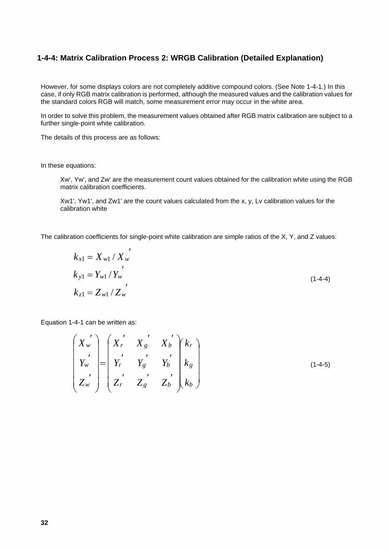
However, for some displays colors are not completely additive compound colors. (See Note 1-4-1.) In this case, if only RGB matrix calibration is performed, although the measured values and the calibration values for the standard colors RGB will match, some measurement error may occur in the white area.
In order to solve this problem, the measurement values obtained after RGB matrix calibration are subject to a further single-point white calibration.
The details of this process are as follows:
In these equations:
Xw', Yw', and Zw' are the measurement count values obtained for the calibration white using the RGB matrix calibration coefficients.
Xw1', Yw1', and Zw1' are the count values calculated from the x, y, Lv calibration values for the calibration white
The calibration coefficients for single-point white calibration are simple ratios of the X, Y, and Z values:
′=
′=
′=
wwz
wwy
wwx
ZZk
YYk
XXk
/
/
/
11
11
11
(1-4-4)
Equation 1-4-1 can be written as:
⎟⎟⎟⎟
⎠
⎞
⎜⎜⎜⎜
⎝
⎛
⎟⎟⎟⎟⎟
⎠
⎞
⎜⎜⎜⎜⎜
⎝
⎛
′′′
′′′
′′′
=
⎟⎟⎟⎟⎟
⎠
⎞
⎜⎜⎜⎜⎜
⎝
⎛
′
′
′
b
g
r
bgr
bgr
bgr
w
w
w
k
k
k
ZZZ
YYY
XXX
Z
Y
X
(1-4-5)
32

Then, the final count values Xw2, Yw2, Zw2 obtained from calibration using single-point white calibration applied to the R, G, B matrix coefficients, equations 1-4-4 and 1-4-5 are combined to obtain:
⎟⎟⎟⎟
⎠
⎞
⎜⎜⎜⎜
⎝
⎛
⎟⎟⎟⎟⎟
⎠
⎞
⎜⎜⎜⎜⎜
⎝
⎛
′′′
′′′
′′′
⎟⎟⎟⎟
⎠
⎞
⎜⎜⎜⎜
⎝
⎛
=
⎟⎟⎟⎟
⎠
⎞
⎜⎜⎜⎜
⎝
⎛
b
g
r
bgr
bgr
bgr
z
y
x
w
w
w
k
k
k
ZZZ
YYY
XXX
k
k
k
Z
Y
X
1
1
1
2
2
2
00
00
00
(1-4-6)
CA series instruments use the method of single-point white calibration applied to the R, G, B matrix coefficients.
References
Y. Ohno, S. W. Brown: Proc. of the IS&T Sixth Color Imaging Conference pp. 65-68 (1998), "Four-Color Matrix Method for Correction of Tristimulus Colorimeters: Part 2"
Patents: Japan Patent (Open for Comments) 6-323910, US Patent No. 4989982
Notes
Note 1-4-1:
The mixing of two or more primary colors.
Here, for a display which uses the primary colors R, G, and B to create a color image, the color is referred to as an "additive primary color" if the XYZ values for the color (for a given white, for example) are the sum of the XYZ values for the R, G, and B primary colors which comprise the color.
33
1-5: Optical System Features
1-5-1: Optical System Features
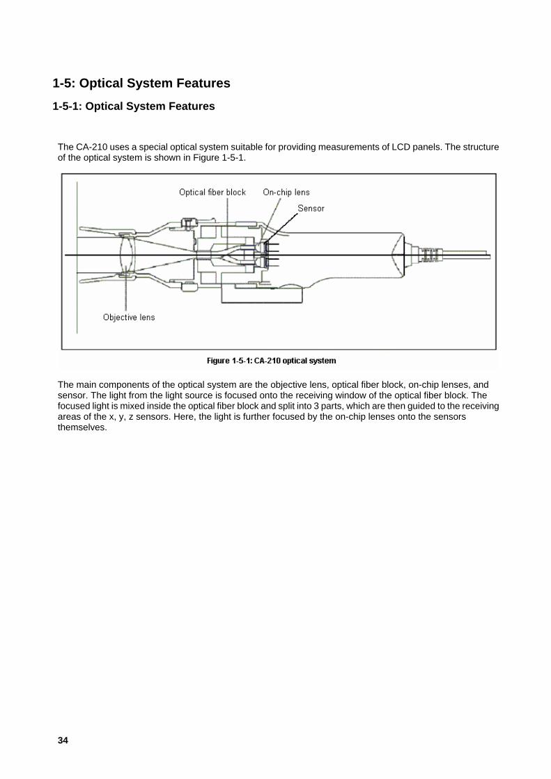
The CA-210 uses a special optical system suitable for providing measurements of LCD panels. The structure of the optical system is shown in Figure 1-5-1.
The main components of the optical system are the objective lens, optical fiber block, on-chip lenses, and sensor. The light from the light source is focused onto the receiving window of the optical fiber block. The focused light is mixed inside the optical fiber block and split into 3 parts, which are then guided to the receiving areas of the x, y, z sensors. Here, the light is further focused by the on-chip lenses onto the sensors themselves.
34

1-5-2: Optical System and Measurement Advantages
1-5-2-1: Low-Luminance Measurement
A key point in making it possible to accurately take measurements at low-luminance levels is to minimize the light loss in guiding the received light to the sensors.
In a conventional system (as shown in Figure 1-5-2), the received light passes through the objective lens and is focused immediately on the 3 sensors (x, y, z sensors). A problem with this method, some of the light is focused on areas other than the sensor, so the light loss is large.
The CA-210 uses optical fibers, so the light loss due to transmission of the light to the sensors is relatively low compared to conventional methods. Specifically, as shown in Figure 1-5-1 in the previous section (and shown again below), the light received by the lens is focused on the optical fiber block receiving window. The light then passes through optical fibers directly to on-chip lenses, which focus the light onto the sensors. As a result of this, light transmission loss is eliminated and measurements at low luminance levels are made possible.
35

1-5-2-2: Narrow Viewing Angle/Uniform Viewing Angle
When a person looks at a display, they view the emitted light within a relatively narrow angle. Because of this, in order to obtain measured values which correspond well with the luminance and chromaticity perceived by a person, it is necessary for the measuring instrument to have the same narrow viewing angle. In addition, since LCDs have viewing-angle characteristics, measurements at different viewing angles will result in different measured values. IEC 61747-6, which defines the measurement method for LCDs, specifies that the viewing angle of the measuring instrument for evaluating LCDs should be within 5°. (The viewing angle is shown by θ1, θ2, θ3 in Figure 1-5-3a and Ψ1, Ψ2, Ψ3 in Figure 1-5-3b.)
The CA-210 has a viewing angle of 5°, and so meets the requirements of the IEC standard.
For a conventional measuring instrument, the relationship between the measuring position and the incident angle on the instrument is as shown in Figure 1-5-3a. For this diagram, the measuring head has been set so that the measurement axis is perpendicular to the surface of the emitting surface of the measurement subject. As shown in Figure 1-5-3a, for a conventional measuring instrument, differences in the measurement position do not result in great differences in the viewing angle itself (shown as by θ1, θ2, θ3 in the figure), but if we look at the incident angle relative to the normal to the emitting surface (shown as a dotted line in the figure), we see that the maximum angles (shown as θ'1 and θ'3 in the diagram) are very different. At the edges of the measurement area, light from far outside the viewing angle is received.
By using a special optical system in the CA-210, the angle of the received light is symmetrical about the normal to the emitting surface for every point within the measuring area (∅27mm), as shown in Figure 1-5-3b. Since the viewing angle of the CA-210 is 5°, the light received would be only the light within ±2.5° relative to the normal to the emitting surface (shown as a dotted line in the figure).
36
1-5-2-3: Reduced Influence of Luminance/Chromaticity Variation
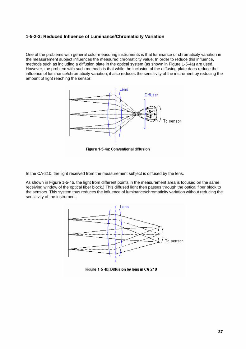
One of the problems with general color measuring instruments is that luminance or chromaticity variation in the measurement subject influences the measured chromaticity value. In order to reduce this influence, methods such as including a diffusion plate in the optical system (as shown in Figure 1-5-4a) are used. However, the problem with such methods is that while the inclusion of the diffusing plate does reduce the influence of luminance/chromaticity variation, it also reduces the sensitivity of the instrument by reducing the amount of light reaching the sensor.
In the CA-210, the light received from the measurement subject is diffused by the lens.
As shown in Figure 1-5-4b, the light from different points in the measurement area is focused on the same receiving window of the optical fiber block.) This diffused light then passes through the optical fiber block to the sensors. This system thus reduces the influence of luminance/chromaticity variation without reducing the sensitivity of the instrument.
37

1-6: Circuit Features
1-6-1: Differences between CA-210 A/D Conversion and Conventional Methods
In a conventional luminance meter or colorimeter, A/D (analog/digital) conversion of the analog output signal from the sensor is often performed using the double-integration method. This method is shown in Figure 1-6-1.
Let's consider a light source which emits light at varying intensity as at the left in Figure 1-6-1.
The light energy of this light source is converted into electrical energy by the sensor and input to the integrator. In the integrator, after charging for a fixed period of time (t1), the charge is drained off. The output from the integrator is as shown at the right in Figure 1-6-1. Since the time (t2) required to completely drain off the charge is proportional to the charge value, a digital value corresponding to the sensor output can be obtained by measuring this time t2.
However, recently the performance of A/D conversion elements has been improving, and the method of direct A/D conversion of the sensor output is starting to be used instead of the double-integration method.
(This method is referred to as "successive A/D method" below.)
As shown in Figure 1-6-2, in this method, A/D conversion of the analog signal output is performed repeatedly during a fixed period of time (t1) and digital values (indicated by • in Figure 1-6-2). The sum of these digital values is then calculated to determine the digital value corresponding to the sensor output.
The CA-210 uses the successive A/D method.
The advantages of this method are described in the following section.
38

1-6-2: Advantages of Successive A/D method
1-6-2-1: Measurement of even lower luminance levels
In order to measure low luminance levels, improved repeatability is essential. It is said that increasing the signal to noise (S/N) ratio is equivalent to improving repeatability.
Increasing the S/N ratio can be done by either of two methods:
1 Increasing the valid signal component.
2 Reducing noise.
In the CA-210, the S/N ratio is increased by using method 2.
In general, it is known that if the A/D value is summed n times, the noise (relative to the signal) is reduced by a factor of . In the CA-210, using the successive A/D method, 100 digital values are obtained and summed for each measurement, resulting in noise being greatly reduced.
1-6-2-2: Reduced measurement time
For example, if the integration time is 100msec:
With the double-integration method, the analog output signal charge time (t1 in Figure 1-6-1, = 100msec) and the charge drain time (t2 in Figure 1-6-1) is necessary.
However, with the A/D method used in the CA-210, only the time to perform A/D conversion repeatedly (t1 in Figure 1-6-2, = 100msec) is necessary.
This helps reduce the measuring time. (To provide even greater speed, a fast CPU is used to help reduce calculation time and USB is used to help reduce communication time.)
1-6-2-3: Flicker measurement
Since the digital value can be obtained as a function of time as shown in Figure 1-6-2, flicker measurement can also be measured.
The CA-210 LCD Flicker Measuring Probe can measure flicker by two different methods. In both cases, the digital values described above are used.
The Contrast Flicker Value, which is calculated as the ratio between the AC component and DC component, can be calculated using the maximum and minimum digital values obtained as a function of time.
The JEITA Method Flicker Value, which is calculated as the frequency component of the subject light source multiplied by the frequency response of the human eye, can be calculated by performing digital Fourier transformation of the digital values obtained over time and performing numerical processing of the results.
39

1-7: LCD Flicker Measurement
1-7-1: What is LCD Flicker?
When an LCD panel is displaying a net or checkerboard pattern image, (such as when shutting down Windows), the screen may seem to shimmer and become extremely hard to view. This shimmering is called "LCD flicker" (hereafter referred to as "flicker"). The mechanism by which flicker occurs is explained in the next section
1-7-1-1: How Flicker Occurs
It is known that continuously supplying a DC image signal to a liquid crystal display device shortens the life of the LCD panel. In addition, LCD devices respond to negative voltages as well as positive voltages. Because of this, generally the polarity of the image signal input to a liquid crystal device is reversed every frame (vertical synchronization period).
Let's consider the case where the same image is displayed on the screen continuously. For the image of each frame, the reference voltage must be equal to the center of amplitude of the image signal, as shown in Figure 1-7-1. However, if the position of the reference voltage is shifted as in Figure 1-7-2, the positive and negative components of the image signal become different. As a result of this, the image signal changes at a frequency equal to 1/2 the frame rate frequency.
For example, if the vertical synchronization frequency is 60Hz, the image signal changes at the frequency of 30Hz. Since this is below the perception threshold frequency for humans, humans perceive shimmering.
If flicker occurs on an LCD, it is extremely annoying to view. In general, the reference voltage of LCD panels is adjusted during the manufacturing process.
40

1-7-1-2: LCD Drive Systems and Images Likely to Cause Flicker
Recently, in order to increase the uniformity of the image display, liquid crystal drive elements which receive the signal input to the LCD device and invert the polarity of the signal for each pixel have been developed and are being used in LCD panels.
There are two types of these inverting drive systems:
Line inversion drive system: The signal polarity is inverted for alternate horizontal lines. This system is currently used in a lot of small LCD panels.
Dot inversion drive system: The signal polarity is inverted for alternate pixels in a horizontal line. If the pixels in a given horizontal line had the polarities positive, negative, positive, ...., then the pixels in the next line would have the polarities negative, positive, negative, ... (checkerboard pattern). This system is currently used in a lot of large-size LCD panels.
If a uniform image fills the entire screen, on an LCD panel using these pixel inversion systems, flicker resulting from the shift in reference voltage described above would occur for the inverted alternate horizontal lines or alternate pixels. In this case, the averaging effect of the human eye results in almost no flicker being perceived.
However, now let's consider the case of a dot-inversion LCD panel displaying a checkerboard pattern (as shown in Figure 1-7-3) where alternating pixels are switched on and off repeatedly. In this case, the pixels which are lit receive the same signal polarity during a given frame period, making inversion of each pixel more likely to occur and causing the entire image to be perceived as flickering.
In the same way, for a line-inversion LCD panel displaying an image of horizontal bars like that shown in Figure 1-7-4, the entire image will be perceived as flickering.
At the beginning of this discussion, we said that the image shown when Windows is shutting down is likely to cause flicker. This is because the image is a checkerboard pattern.
41

1-7-1-3: Flicker Measurement Examples
Large amount of flicker
JEITA measurement value: -14.5dB
AC/DC measurement value: 68.4%
Measurement AVI file: F_Big.avi
Medium amount of flicker
JEITA measurement value: -22.7dB
AC/DC measurement value: 27.8%
Measurement AVI file: F_Medium.avi
Small amount of flicker
JEITA measurement value: -40.9dB
AC/DC measurement value: 2.7%
Measurement AVI file: F_Small.avi
Note: Microsoft Media Player is necessary to play the measurement AVI files. Media Player is a registered trademark of Microsoft Corp.
Reference:
Takawa, Mikiyu, Display Monthly Vol. 8, No. 6 (June 2002): 51
42

1-7-2: Flicker Measurement Methods
1-7-2-1: Flicker Measurement
Figure 1-7-5 shows the relationship between luminance and time when flicker occurs. As can be seen in this figure, the luminance changes cyclically; it is clearly recognized that the higher the amplitude of this cycle, the greater the apparent flickering.
In addition, the period of this luminance fluctuation is the same as twice that of the vertical synchronization signal of the display. (See section 1-7-1: What is LCD Flicker?)
The methods for measuring flicker can be broadly classified into the following two methods:
1 Measure the DC and AC components of the luminance fluctuation and determine flicker from the ratio between the two components.
2 Analyze the frequency component of the luminance fluctuation and determine flicker from the ratio between the DC component and the maximum AC component at any frequency.
The CA-210 LCD Flicker Measuring Probe can measure flicker using either the contrast method for method (1) or the JEITA method for method (2).
The characteristics of each method are shown in Table 1. The method to be used should be decided according to the measurement purpose. In general, the contrast method is suitable for adjustment and inspection during the manufacture of LCD panels, and the JEITA method is suitable for use in the development and design of LCD panels.
Contrast Method JEITA methodMeasurement speed
Fast measurement speed (16 times/sec.) Slow measurement speed (0.5 times/sec.)
Performance features
The relative maximum and minimum of the f licker can be understood.The f requency response characteristics of the human eye are not taken into consideration
The absolute value of the f licker can be understood.The f requency response characteristics of the human eye are taken into consideration.
Table 1-7-1: Characte ris tics of flicker m easurem ent m ethods
Both methods will be explained in this section.
43

1-7-2-2: Explanation of Flicker Measurements by Contrast Method
1-7-2-2-1: Overview of Flicker Measurement by Contrast Method
When the luminance level of a display fluctuates as shown in Figure 1-7-6, it can be thought of as an AC component added to a DC component. This flicker amount defined as (AC component)/(DC component) is called the "contrast method flicker value" (referred to hereafter as the "contrast flicker value").
In the contrast method, since the AC component and DC component are defined as:
( ) 2 component DC component AC
minmax
minmaxVV
VV+=
−=
the flicker value can be calculated using Equation 1 below: ( )( ) [ ]
( )( ){ } [ ]%100
2
%100component DCcomponent AC lueFlicker va
minmax
minmax ×+−
=
×=
VVVV
(1-7-1)
44

1-7-2-2-2: Data Processing for Contrast Method (Details)
The flow of processes which take place inside the instrument from the time the sensor data output is obtained until the flicker value has been calculated will be explained using Figure 1-7-7 below.
(A) to (C) The output signal from the luminance sensor is electrically processed to remove the high-frequency components to obtain the signal to be used for calculating flicker.
(C) to (D) A/D conversion is performed for a specified time (t1) on the analog signal obtained after removing the high-frequency components to obtain the digital data required for calculations (indicated by • in (D)).
(D) to (E) The maximum and minimum values in the digital data are determined and set as Vmax and Vmin respectively.
45

(E) to (G) These values are then used to calculate the (AC component)/(DC component) ratio and the flicker value according to Equation 1. During the calculation of the AC component, compensation for the reduction which occurred during processing by the low-pass filter is performed according to the frequency of the AC component.
46

1-7-2-2-3: Differences from the VESA Standard Contrast Method (Details)
VESA 305-5 specifies a method for measuring flicker based on the ratio between the AC component and the DC component. This section will explain the differences between the VESA specified contrast flicker method and the contrast flicker method used by the CA-210 LCD Flicker Measuring Probe.
Put simply, the VESA standard reflects the frequency response characteristics of the human eye, and the CA-210 LCD Flicker Measuring Probe does not reflect such characteristics in order to provide high-speed measurements.
The VESA standard defines two equations for calculating the flicker value: (See Note 1-7-1.)
( ) [ ]%100max
minmax ×−
VVV
........................(1-7-2)
( )( ){ } [ ]%100
2minmax
minmax ×+−VVVV
(1-7-3)
The Vmax and Vmin values defined here include the influence of the frequency response characteristics of the human eye. (See Note 1-7-2.) Further, Equation 1-7-3 is intended for use when the flicker value is small (13% or lower).
To be more specific, in order to obtain the Vmax and Vmin used here, the sensor output signals are processed by a low-pass filter having the frequency response characteristics of the human eye, and the maximum and minimum values of those processed signals are determined.
The frequency response characteristics of the human eye are shown in Figure 1-7-8 and Table 1-7-2.
The contrast flicker calculations used by the CA-210 system are the same as Equation 1-7-3, but the CA-210 LCD Flicker Measuring Probe does not include the influence of the spectral response of the human eye.
However, the flicker frequency is 1/2 the vertical synchronization frequency of the LCD. (See section 1-7-1: What is LCD Flicker?) The frequency of the AC component f0 can be determined from the vertical synchronization frequency of the LCD. On the other hand, the reduction ratio of f0 can be calculated using Table 1-7-2. Therefore, the flicker value conforming to the VESA standard can be calculated from the contrastflicker value.
dB Ratio0 0 1.000
10 0 1.00020 0 1.00030 -3 0.70840 -6 0.50150 -12 0.25160 -40 0.010
Table 1-7-2: Freque ncy res ponse characte ris tics of the hum an eye
FactorFrequency(Hz)
47

For example, if the vertical synchronization signal is 60Hz and the contrast flicker value is 10.0%, then the AC component of the flicker would be
( ) [ ]Hz302160 =×
The reduction ratio for the AC component due to the frequency response characteristics of the human eye (from Table 2) would be 0.708. Therefore, the flicker value conforming to the VESA standard would be
[ ]%1.7708.010 ≈×
Notes
Note 1-7-1:
Equation 1-7-3 is actually written
( ) [ ]%100dc
minmax ×−
VVV
Here, we are using
( ) 2minmaxdc VVV +=
Note 1-7-2:
The human perception of a flashing light. The characteristic of the human eye to have a sensitivity to flashing light which decreases gradually as frequency increases from around 30Hz; at over 60Hz, the flashing is no longer perceptible to the eye.
48

1-7-2-3: Explanation of Flicker Measurements by JEITA Method
1-7-2-3-1: Overview of Flicker Measurement by JEITA Method
The JEITA method of flicker measurement is a method for quantifying the flicker value while accurately reflecting the frequency response characteristics of the human eye.
When the luminance level of a display is fluctuating as shown in Figure 1-7-6, the flicker light can be considered to be several frequency components added to a DC component. Therefore, first, the luminance fluctuation data over time is separated into its frequency components (DC component and each AC component; Note 1-7-3). Next, each frequency component is converted into a value which takes into consideration the frequency characteristics of the human eye.
Of the various frequency components obtained, the power spectrum of the component other than the 0Hz (DC) component with the maximum power spectrum is set as Px and the power spectrum of the DC component is set as P0 and Equation 4 below is used to determine the flicker value (referred to hereafter as the JEITA flicker value).
( )010log10 lueFlicker va PPx×= (1-7-4)
Notes
Note 1-7-3:
Under the condition that the flicker component is only the component at a frequency of 1/2 the vertical synchronization frequency. If this condition is not satisfied and other frequency components are included, those other frequency components will be a source of measurement error.
49
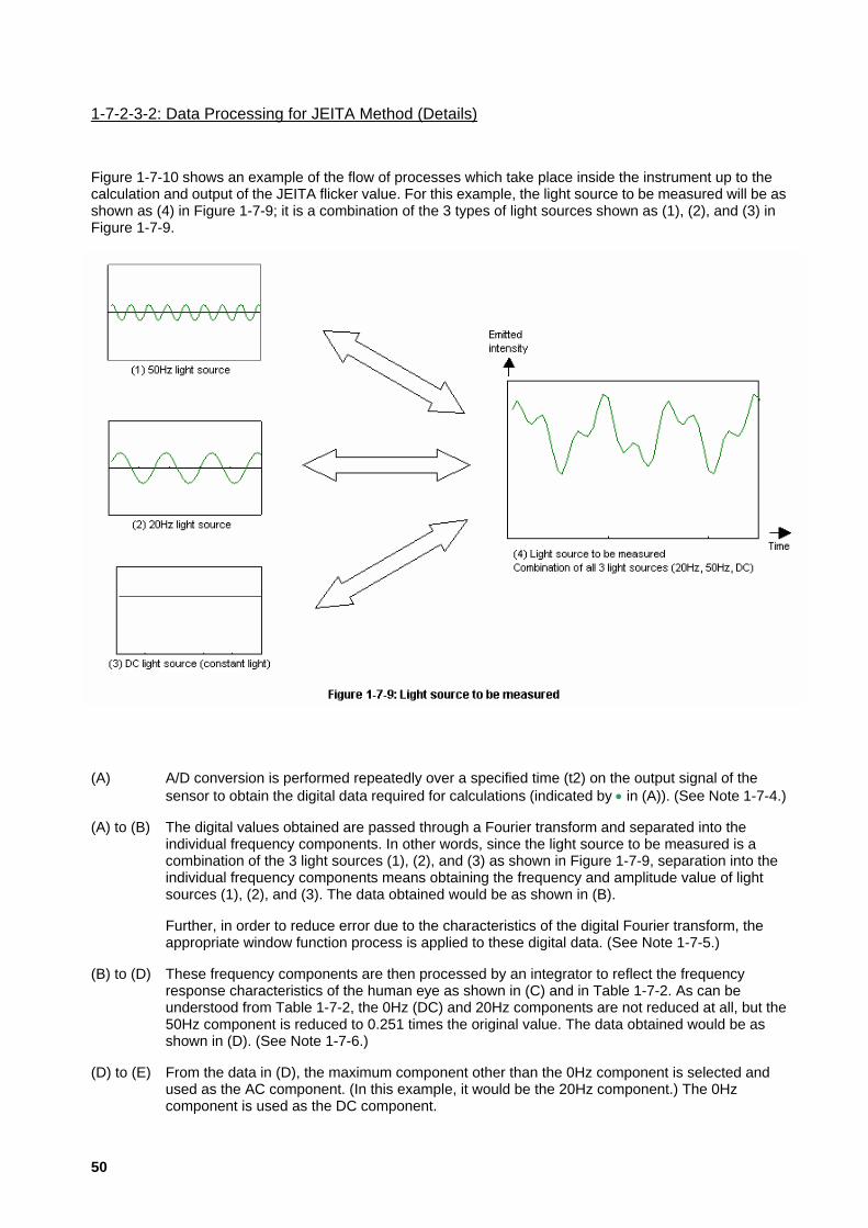
1-7-2-3-2: Data Processing for JEITA Method (Details)
Figure 1-7-10 shows an example of the flow of processes which take place inside the instrument up to the calculation and output of the JEITA flicker value. For this example, the light source to be measured will be as shown as (4) in Figure 1-7-9; it is a combination of the 3 types of light sources shown as (1), (2), and (3) in Figure 1-7-9.
(A) A/D conversion is performed repeatedly over a specified time (t2) on the output signal of the sensor to obtain the digital data required for calculations (indicated by • in (A)). (See Note 1-7-4.)
(A) to (B) The digital values obtained are passed through a Fourier transform and separated into the individual frequency components. In other words, since the light source to be measured is a combination of the 3 light sources (1), (2), and (3) as shown in Figure 1-7-9, separation into the individual frequency components means obtaining the frequency and amplitude value of light sources (1), (2), and (3). The data obtained would be as shown in (B).
Further, in order to reduce error due to the characteristics of the digital Fourier transform, the appropriate window function process is applied to these digital data. (See Note 1-7-5.)
(B) to (D) These frequency components are then processed by an integrator to reflect the frequency response characteristics of the human eye as shown in (C) and in Table 1-7-2. As can be understood from Table 1-7-2, the 0Hz (DC) and 20Hz components are not reduced at all, but the 50Hz component is reduced to 0.251 times the original value. The data obtained would be as shown in (D). (See Note 1-7-6.)
(D) to (E) From the data in (D), the maximum component other than the 0Hz component is selected and used as the AC component. (In this example, it would be the 20Hz component.) The 0Hz component is used as the DC component.
50
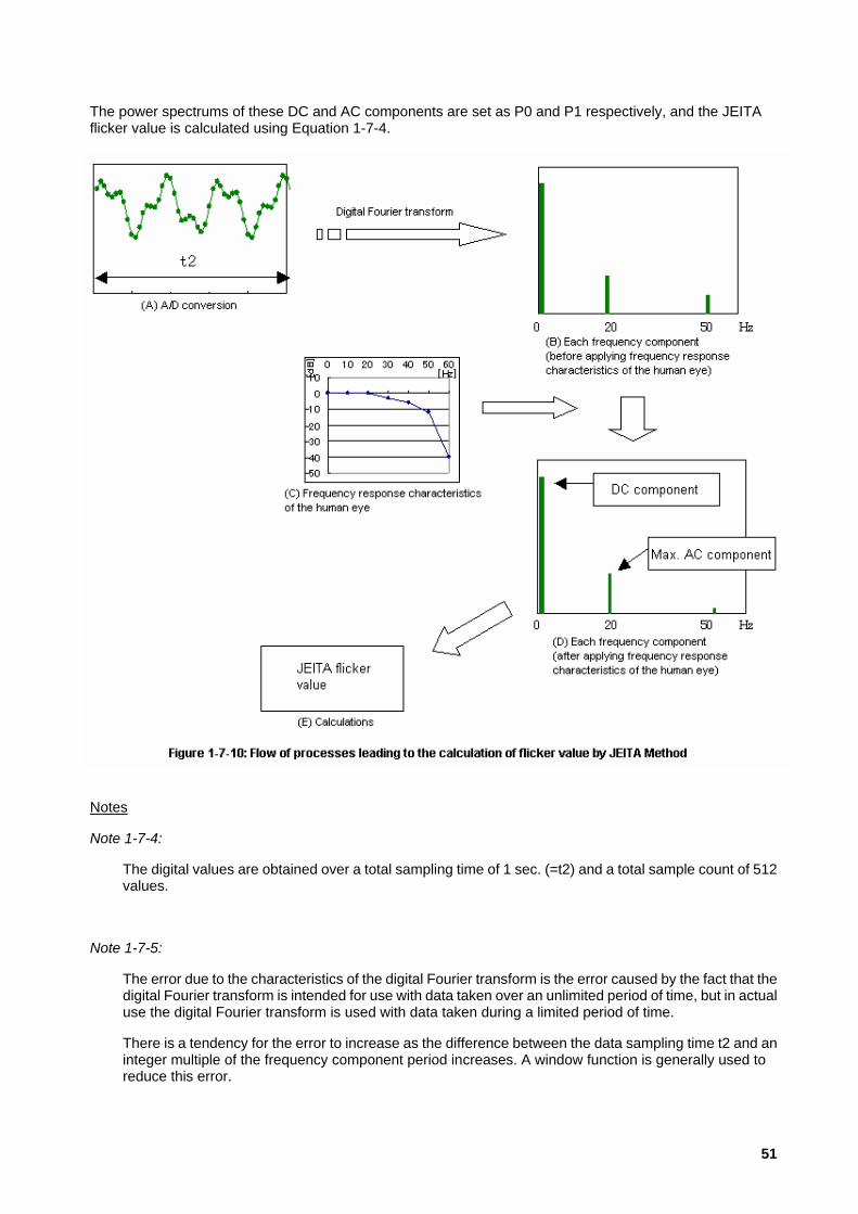
The power spectrums of these DC and AC components are set as P0 and P1 respectively, and the JEITA flicker value is calculated using Equation 1-7-4.
Notes
Note 1-7-4:
The digital values are obtained over a total sampling time of 1 sec. (=t2) and a total sample count of 512 values.
Note 1-7-5:
The error due to the characteristics of the digital Fourier transform is the error caused by the fact that the digital Fourier transform is intended for use with data taken over an unlimited period of time, but in actual use the digital Fourier transform is used with data taken during a limited period of time.
There is a tendency for the error to increase as the difference between the data sampling time t2 and an integer multiple of the frequency component period increases. A window function is generally used to reduce this error.
51

As a result, the frequency component detection accuracy increases, but conversely, the detection resolution decreases.
For example, if there is a frequency component (for example, at 30Hz) present as shown in the figure below, if the digital Fourier transform is used without the window function, a value which is lower than the true value is calculated as shown in (B) of the figure. On the other hand, if the digital Fourier transform is used with the window function, the 30Hz component can be accurately obtained, but components to either side of the 30Hz component are also output. However, since the true value of the 30Hz component is obtained, the JEITA flicker value can be determined accurately.
Note 1-7-6:
The process of calculating flicker is performed as follows:
JEITA standard
1 Obtain measured luminance signal.
2 Pass through integrator.
3 Pass through FFT analyzer.
4 Calculate power spectrum.
CA-210 LCD Flicker Measuring Probe
1 Obtain measured luminance signal.
2 Pass through FFT analyzer.
3 Pass through integrator.
4 Calculate power spectrum.
The order of "Pass through integrator" and "Pass through FFT analyzer" is reversed.
However, since the data which is input to step 4 ("Calculate power spectrum") is the same in both cases, the same flicker value will be obtained from either process. In other words, equivalent data processing is being performed.
52

References:
VESA 305-4, 305-5
EIAJ ED-2522
Shigeo Minami, Waveform Data Processing for Optical Measurements (CQ Publishing)
Shougo Nakamura, Digital Fourier Transforms (Tokyo Institute of Electronics Publications)
53

1-7-2-3-2-1: Differences from Contrast Method
When the light source is like that shown as (4) in Figure 1-7-9, the contrast method uses the sensor output signal "as is" and uses the difference between the maximum and minimum values (as indicated by the arrows in the top diagram in Figure 1-7-11) as the AC component. On the other hand, in the JEITA method, since the signal is separated into its frequency components, only the maximum component (the 20Hz component in the example) is selected, and the difference between its maximum and minimum values (as indicated by the arrows in the bottom diagram in Figure 1-7-11) is used as the AC component. Another difference is that if the frequency of the maximum AC component is greater than 20Hz, the reduction ratio due to the frequency characteristics of the human eye is taken into consideration.
54

1-7-2-3-3: CA-210 Data Processing for JEITA Method (Details)
The flow of processes in the CA-210 LCD Flicker Measuring Probe from obtaining the sensor output, passing it through the digital Fourier transform process, and calculating the JEITA flicker value will be explained in the following sections.
55

1-7-2-3-3-1: Equation Used by CA-210 for JEITA Method
The CA-210 calculates the JEITA flicker value using the following equation:
⎟⎟⎠
⎞⎜⎜⎝
⎛
×××
×)0()0(
)()(2log20FFTweight
kFFTkweight
(1-7-5)
where
k: Frequency
weight(k): Integrator constant for frequency k
FFT(k): Maximum value of weight(k) × FFT(k) obtained from the FFT output for frequency k (k>0)
FFT(0): FFT output for the DC component
56

1-7-2-3-3-2: Explanation of JEITA Method Equation
The flicker value obtained by the JEITA Flicker Method is defined by the following equation:
⎟⎟⎠
⎞⎜⎜⎝
⎛×
0log10
PPx
(1-7-6)
where
Px: Maximum power spectrum of AC component after passing through integrator
P0: Power spectrum of DC component after passing through integratorIm
(From EIAJ ED2522)
The relationship between ratios for the FFT output and the power spectrum for the DC component (x=1) and the AC component (x=sin(t)) is shown in the following table:
(1) DC component (x=1) (2) AC component (x=sin(t))FFT output 1 0.5Pow er spectrum 2 1
Table 1-7-3: Re lationship be tw een ratios for FFT output and pow er spectrum
For (1) and (2), they should be the same from the concept of amplitude, but the FFT outputs have the ratio 1:0.5, so by doubling only the frequency component, they can be made the same (or in other words, the FFT outputs the AC component as 1/2 the DC component).
Therefore, the correlation between the DC and AC components is: Amplitude of frequency component 2 × FFT(k) (=Ak) (1-7-7) Amplitude of DC component FFT(0) (=A0) (1-7-8)
When converting this to the power spectrum, since the DC component is the square of the amplitude and the AC component is 1/2 the square of the amplitude, Equation 1-7-6 becomes:
( )
( )
⎟⎟⎠
⎞⎜⎜⎝
⎛ ××=
⎟⎟⎟
⎠
⎞
⎜⎜⎜
⎝
⎛ ××=
⎟⎟⎠
⎞⎜⎜⎝
⎛ ××=
)0()(2log20
)0()(2log10
)0(2/)(2log10
2
2
2
2
wFFTkwFFT
wFFTkwFFT
wFFTkwFFT
(1-7-9)
where
wFFT(k) = weight(k) × FFT(k)
wFFT(0) = weight(0) × FFT(0)
and thus we end up with Equation 1-7-5.
57

1-7-2-3-3-3: Additional Information Regarding JEITA Equation
If we think about the effective value, since we can divide only the AC value by in Equation 1-7-6, we get:
( )⎟⎟⎟
⎠
⎞
⎜⎜⎜
⎝
⎛×
2
2
02log10
AAk
(1-7-10)
where Ak and A0 are the amplitudes of the AC component and DC component respectively.
If we then apply Equations 7 and 8, we get:
( )( )( )
( )( ) ⎟
⎟⎠
⎞⎜⎜⎝
⎛ ××=
⎟⎟⎟
⎠
⎞
⎜⎜⎜
⎝
⎛ ××=
02log20
02log10 2
2
wFFTkwFFT
wFFTkwFFT
(1-7-11)
which is the same as Equation 1-7-5. In other words, Equation 1-7-5 corresponds to the effective value.
58

1-7-2-3-3-4: Differences from the VESA Standard
VESA 305-4 defines a flicker measurement method based on the separation of the AC component into its frequency components. In the standard, the flicker value is defined by the following equation:
⎟⎟⎠
⎞⎜⎜⎝
⎛ ××
)0()(2log20
wFFTkwFFT
(1-7-12)
(The amplitudes of the AC and DC components are just squared.)
If we compare this to Equation 1-7-5, we see that the value inside the log function is different.
In order to calculate the VESA flicker value from the JEITA flicker value, we must do the following:
( )( )
( )( ) ( )
( ) ( )2log20lueflicker vaJEITA
2log200
2log20
02log20 lueflicker vaVESA
×+=
×+⎟⎟⎠
⎞⎜⎜⎝
⎛ ××=
⎟⎟⎠
⎞⎜⎜⎝
⎛ ××=
wFFTkwFFT
wFFTkwFFT
(1-7-13)
In other words, we can obtain the VESA flicker value by adding approximately 3.01[dB] (=20 × log ) is added to the JEITA flicker value.
59
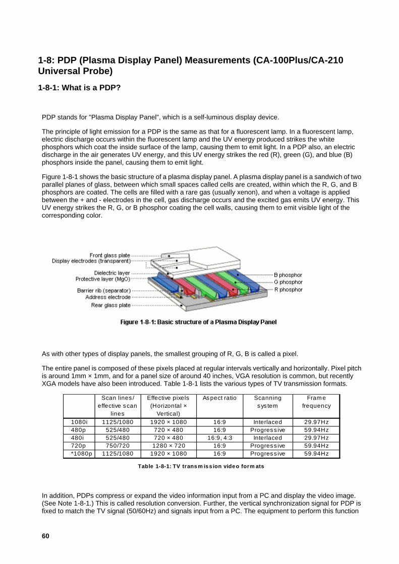
1-8: PDP (Plasma Display Panel) Measurements (CA-100Plus/CA-210 Universal Probe) 1-8-1: What is a PDP?
PDP stands for "Plasma Display Panel", which is a self-luminous display device.
The principle of light emission for a PDP is the same as that for a fluorescent lamp. In a fluorescent lamp, electric discharge occurs within the fluorescent lamp and the UV energy produced strikes the white phosphors which coat the inside surface of the lamp, causing them to emit light. In a PDP also, an electric discharge in the air generates UV energy, and this UV energy strikes the red (R), green (G), and blue (B) phosphors inside the panel, causing them to emit light.
Figure 1-8-1 shows the basic structure of a plasma display panel. A plasma display panel is a sandwich of two parallel planes of glass, between which small spaces called cells are created, within which the R, G, and B phosphors are coated. The cells are filled with a rare gas (usually xenon), and when a voltage is applied between the + and - electrodes in the cell, gas discharge occurs and the excited gas emits UV energy. This UV energy strikes the R, G, or B phosphor coating the cell walls, causing them to emit visible light of the corresponding color.
As with other types of display panels, the smallest grouping of R, G, B is called a pixel.
The entire panel is composed of these pixels placed at regular intervals vertically and horizontally. Pixel pitch is around 1mm × 1mm, and for a panel size of around 40 inches, VGA resolution is common, but recently XGA models have also been introduced. Table 1-8-1 lists the various types of TV transmission formats.
Scan lines /effective scan
lines
Effective pixels(Horizontal ×
Vertical)
Aspect ratio Scanning sys tem
Fram e frequency
1080i 1125/1080 1920 × 1080 16:9 Interlaced 29.97Hz480p 525/480 720 × 480 16:9 Progress ive 59.94Hz480i 525/480 720 × 480 16:9, 4:3 Interlaced 29.97Hz720p 750/720 1280 × 720 16:9 Progress ive 59.94Hz*1080p 1125/1080 1920 × 1080 16:9 Progress ive 59.94Hz
Table 1-8-1: TV transm iss ion video form ats
In addition, PDPs compress or expand the video information input from a PC and display the video image. (See Note 1-8-1.) This is called resolution conversion. Further, the vertical synchronization signal for PDP is fixed to match the TV signal (50/60Hz) and signals input from a PC. The equipment to perform this function
60

together with the resolution conversion mentioned above is called a multi-scan converter, and is built into the PDP.
Next, the stepped display method will be explained.
In order to increase the brightness of PDPs, the memory function of the cells is used and line progressive addressing/full-screen simultaneous emission is performed. (See Note 1-8-2.) Figure 1-8-2 shows an example of the stepped display method. In this example, a single TV vertical scan period (= 1 TV field) is divided into 8 subfields. If the length of the emission time is set to powers of 2 (1:2:4:8:16:32:64:128), the combination of these allows 256 steps to be displayed.
In other words, in a PDP, the step is changed by changing the pulse width of the emission period. (See Note 1-8-3.)
In the figure, the horizontal axis is time and the vertical axis is the scanning/discharge standby electrode number. This number corresponds to the pixel number in the vertical direction; for this example, a VGA panel is used.
Each subfield consists of the address period to select which pixel to light and the discharge standby period (sustain period) for the pulse width corresponding to the specified luminance ratio for only the selected pixel.
This kind of stepped display method is called subfield drive method, but it has several display problems which are peculiar to it. The most typical display problem is dynamic false contour images. (See Note 1-8-4.) There are a variety of display methods to reduce display problems like this; in actuality, the methods used are not as simple as the model shown in Figure 1-8-2, and they will also probably continue to change in the future.
Notes
Note 1-8-1:
For the VGA PDP used in the example, signals for SVGA or higher resolutions are compressed for display.
61

Note 1-8-2:
The cell can operate in a so-called bistable condition: Once a signal to light the cell has been applied, the cell remains lit even after the "light" signal has been removed; once a signal to extinguish the cell has been applied, the cell remains extinguished even after the "extinguish" signal has been removed.
Note 1-8-3:
For a CRT, the pixel luminance can be controlled by controlling the intensity of the electron beam (analog quantity control), but since for a PDP it is not possible to control the luminance by controlling the saturation of the UV energy (such as by controlling the current), the luminance is changed by changing the length of the emission period (digital quantity control).
Note 1-8-4:
For a moving image, when the human eye is following that image, the emitting portions and non-emitting portions of the subfields before and after the image appear to melt together, so that a band of color which should not actually be there is visible.
62

1-8-2: Relation to Chromatic Luminance Meter
When the light from a PDP with a variable pulse width is received by a sensor, if the time constant of the sensor control circuit is set to 0, the rectangular waveform shown in Figure 1-8-2, where the signal is 0 or 1, would be obtained and accurate measurement would not be possible. (See Note 1-8-5.) In other words, the difference between the peak value and the average value would become exceedingly large, and since the timing range of the circuit could not be used effectively, the S/N ratio would be very poor. In addition, since the peak would be saturated, absolute-value error would occur.
Therefore, the time constant of the circuit is set to a suitable value so that a normal analog wave is obtained. (See Note 1-8-6.)
In 1-8-1: What is a PDP?, the principle of light emission by a PDP, in which the UV energy created by a gas discharge strikes phosphors and causes them to emit light, was explained.
However, since at the current time the light emission efficiency of PDPs is low, the majority of the energy is converted to heat, and at maximum luminance the temperature exceeds 40°C. In order to eliminate the influence of this increase in temperature, the CA-100Plus series/CA-210 Universal Measuring Probe has a temperature sensor in the measuring probe to perform accurate temperature compensation and provide measurements which are not influenced by the temperature of the screen surface.
Notes
Note 1-8-5:
Actually, during the sustain period, the cell is switched on and off at a frequency of several dozen KHz, and control is performed by changing the stepped peak luminance, etc. by varying the frequency or the duty cycle. As a result of this, the actual waveform of the received light is more complicated.
63

Note 1-8-6:
Two CA-100Plus series probes with different measuring ranges (Standard Probe, High-Luminance Probe) are available. The specifications for each are shown in the table below:
Item CA-100Plus (Standard Probe) CA-100PlusH (High-Lum inance Probe)
Measurem ent range 0.05 to 1000cd/m 2 0.05 to 2000cd/m 2
Accuracy 0.05 to 1000cd/m 2: ±2% ±1 digit (Calibration CRT at D65)
0.05 to 2000cd/m 2: ±2% ±1 digit (Calibration CRT at D65)
Repeatability 0.05 to 1000cd/m 2: ±2% ±1 digit (2σ)
0.05 to 2000cd/m 2: ±2% ±1 digit (2σ)
Measurem ent range 0.05 to 1000cd/m 2 0.05 to 2000cd/m 2
0.05 to 0.09cd/m 2: ±0.008 (Calibration CRT at D65)
0.05 to 0.19cd/m 2: ±0.006 (Calibration CRT at D65)
0.10 to 0.39cd/m 2: ±0.006 (Calibration CRT at D65)
0.20 to 0.49cd/m 2: ±0.004 (Calibration CRT at D65)
0.40 to 0.99cd/m 2: ±0.004 (Calibration CRT at D65)
0.50 to 1000cd/m 2: ±0.003 (Calibration CRT at D65)
1.00 to 2000cd/m 2: ±0.003 (Calibration CRT at D65)
Calibration CRT (D65, 40cd/m 2): ±0.002 (White) ±0.004 (R, G, B)
Calibration CRT (D65, 40cd/m 2): ±0.002 (White) ±0.004 (R, G, B)
(CRT at D65) (CRT at D65)0.05 to 0.09cd/m 2: 0.009 (2σ)
0.05 to 0.19cd/m 2: 0.006 (2σ)
0.10 to 0.39cd/m 2: 0.006 (2σ)
0.20 to 0.49cd/m 2: 0.002 (2σ)
0.40 to 0.99cd/m 2: 0.002 (2σ)
0.50 to 1000cd/m 2: 0.001 (2σ)
1.00 to 2000cd/m 2: 0.001 (2σ)
Lum inance
Chrom aticityAccuracy
Repeatability
64

2: Definitions of Accuracy Standards and Repeatability 2-1: Definition of Luminance/Chromaticity Accuracy Standards and Repeatability
The accuracy specifications for the CA-210 are shown in Table 2-1-1 below. The meanings of these specifications will be explained in the following sections.
Measurement range 0.10 to 1000cd/m2
Accuracy ±2% ±1 digit (Calibration LCD at 6500K and 9300K; Luminance = 0.10 to 1000cd/m2)
Repeatability 0.2%±1 digit (Luminance = 0.1 to 0.99cd/m2)0.1%±1 digit (Luminance = 1.00 to 1000cd/m2)
Measurement range 0.10 to 1000cd/m2
Accuracy ±0.005 (Calibration LCD at 6500K and 9300K; Luminance = 0.10 to 4.99cd/m2)
±0.004 (Calibration LCD at 6500K and 9300K; Luminance = 5.00 to 19.99cd/m2)
±0.003 (Calibration LCD at 6500K and 9300K; Luminance = 20.00 to 1000cd/m2)
±0.002 (±0.004 for primary color) (Calibration LCD at 6500K and 9300K; Luminance = 160cd/m2)
Repeatability 0.010 (2σ) (Calibration LCD at 6500K and 9300K; Luminance = 0.10 to 0.19cd/m2)
0.005 (2σ) (Calibration LCD at 6500K and 9300K; Luminance = 0.20 to 0.49cd/m2)
0.002 (2σ) (Calibration LCD at 6500K and 9300K; Luminance = 0.50 to 0.99cd/m2)
0.001 (2σ) (Calibration LCD at 6500K and 9300K; Luminance = 1.00 to 1000cd/m2)
Luminance
Chromaticity
Table 2-1-1: CA-210 accuracy and repeatability specifications
65

2-1-1: Accuracy
2-1-1-1: Definition of Accuracy
The traceability system of the CA-210 can be traced to a national standard. (See section 2-1-4: Traceability later in this document.)
Accuracy is defined as the difference from the measurement values obtained using the CA-210 Standard Unit which has been calibrated according to the CA-210 traceability system. However, the definition of accuracy does not include repeatability error, and therefore the average of several measurements is used.
66
2-1-1-2: Luminance Range for Certified Accuracy
The CA-210 can measure luminance to the certified accuracy within the range of 0.1 to 1000 cd/m2. (See Note 2-1-1.)
The light sources for which the accuracy can be certified are light sources which do not change their emitted spectral power distribution or emission distribution characteristics even if the luminance changes.
Notes
Note 2-1-1:
The minimum luminance for measuring the contrast of an LCD monitor is generally around 0.5cd/m2 . Since the accuracy of the CA-210 is certified for a sufficiently low luminance, its performance is sufficient for inspection and evaluation of LCD monitors.
67

2-1-1-3: Light Sources for Certified Accuracy (Details)
For tristimulus colorimeters, even if no absolute-value error occurs when measuring a certain light source (display), absolute-value error will occur if a different light source is measured. Also, even when measuring the same light source, if a different color is measured, absolute-value error may occur. (See section 1-2-3: Absolute-Value Error for Tristimulus Colorimeters.)
Therefore, for tristimulus colorimeters, the light source for which accuracy is certified is listed in the catalog. The accuracy of the CA-210 is certified using Konica Minolta's standard LCD monitor.
If the difference between the emitted spectral power distributions of the light source for which accuracy is certified and the light source to be measured is small, the absolute-value error will also be small. Furthermore, the spectral characteristics of even different models of LCD monitors are very similar (see Figure 2-1-1). Therefore, when the CA-210 is used to measure an LCD monitor, it can provide high measurement accuracy (small absolute-value error).
Generally, Standard Illuminant A is used as the light source for which the accuracy of tristimulus colorimeters is certified. On the other hand, since the spectral characteristics of LCD monitors are very different from those of Standard Illuminant A (see Figure 2-1-1), if a colorimeter for which the accuracy was certified using Standard Illuminant A is used to measure an LCD monitor, there is a tendency for the absolute-value error and inter-instrument error to increase. (See Note 2-1-2.)
The above applies to both luminance and chromaticity.
Notes
Note 2-1-2:
The quantitative test results when the absolute-value error which would occur when measuring 5 models of LCD monitors using calibration to Standard Illuminant A and calibration to an LCD monitor (the Konica Minolta standard LCD monitor) are shown in Tables 2-1-3a and 2-1-3b respectively. Here, the quantitative test was performed based on the spectral power distribution characteristics of each light source as actually measured. The chromaticity of the LCD monitor was set to white (6500K to 9300K).
68

∆x ∆y ∆x ∆y Standard Illuminant
A 0.0000 -0.0000 Konica Minolta Standard LCD 0.0000 0.0000
LCD A -0.0085 -0.0027 LCD A -0.0004 0.0016 LCD B -0.0087 -0.0048 LCD B -0.0004 -0.0010 LCD C -0.0090 -0.0022 LCD C -0.0005 -0.0015 LCD D -0.0084 -0.0017 LCD D -0.0001 0.0017 LCD E -0.0081 -0.0042 LCD E -0.0016 0.0012
Table 2-1-3a: Measurement error for 5 LCDs after calibration to Standard Illuminant A Table 2-1-3a: Measurement error for 5 LCDs after
calibration to Konica Minolta Standard LCD
From these results, it can be seen that compared to the small absolute-value error for xy of less than approx. 0.002 which was obtained from calibration to an LCD monitor, the absolute-value error from calibration to Standard Illuminant A is much larger at 0.009.
69

2-1-2: Repeatability
2-1-2-1: Definition of Repeatability
The repeatability of the CA-210 is defined as twice the standard deviation (2 σ ) for multiple measurements under the same conditions.
70

2-1-2-2: Light Sources for Certified Repeatability (Details)
The light source for which the repeatability of the CA-210 is certified is LCD monitors.
The measured color is specified as 6500K and 9300K. When other colors are measured, the repeatability will be different. The repeatability results for actual measurements of white (6500K) and the three primary colors are shown in Table 2-1-2. (Three CA-210 units were evaluated.)
x y x y LvNo. 1 0.0003 0.0003 0.6318 0.3274 1.09No. 2 0.0005 0.0005 0.6322 0.3269 1.09No. 3 0.0003 0.0002 0.6326 0.3257 1.09No. 1 0.0002 0.0005 0.2868 0.5861 1.38No. 2 0.0002 0.0004 0.2869 0.5860 1.38No. 3 0.0002 0.0004 0.2871 0.5853 1.38No. 1 0.0001 0.0000 0.1464 0.0494 1.01No. 2 0.0001 0.0000 0.1465 0.0496 1.02No. 3 0.0001 0.0001 0.1461 0.0493 1.02No. 1 0.0001 0.0002 0.3089 0.3243 1.38No. 2 0.0002 0.0002 0.3092 0.3241 1.38No. 3 0.0002 0.0002 0.3096 0.3239 1.39
Chromatic ity/luminance at time of measurementMeasured
colorBody No.
Repeatability (2σ)
W
Table 2-1-2: Results of actual te s t of re peatability for pr im ary colors
R
G
B
From these results, it can be seen that the repeatability for R and G are somewhat worse than for W, but the repeatability for B is better. (See Note 2-1-3.)
Notes
Note 2-1-3:
The main factor which determines repeatability is the size of the X, Y, Z sensor output. As each output increases, the repeatability improves.
The results shown in Table 2-1-2 were obtained with the Lv value (Y sensor output) kept almost constant. Therefore, the differences in the repeatability values are due to the differences in the X and Z sensor outputs.
The sensor outputs when each color was measured are shown in Table 2-1-4.
X Y ZR 1.9 1.0 0.1G 0.5 1.0 0.2B 2.9 1.0 16.1W 1.0 1.0 1.1
Sensor Output Ratios
Table 2-1-4: Se nsor output ratios w hen m easuring pr im ary colors
When R was measured, the X sensor output was higher compared to when W (white) was measured, but since the Z sensor output was exceedingly small, the repeatability was lower compared to the W measurements.
When G was measured, since both the X and Z sensor outputs were lower compared to when W was measured, the repeatability was lower compared to the W measurements.
When B was measured, since the sensitivity of the Y sensor to B is low, when Lv was set to 1 , the outputs from both the X and Z sensors were higher compared to W, resulting in higher repeatability compared to the W measurements.
71

2-1-3: Measurement Accuracy
2-1-3-1: What is Measurement Accuracy?
It was stated previously that accuracy does not include repeatability. In other words, accuracy and repeatability are defined separately.
Therefore, as shown in Figure 2-1-2, for a single measurement, the measured value will be within the range defined by (accuracy error + repeatability error) from the true value.
72
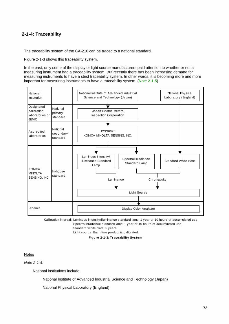
2-1-4: Traceability
The traceability system of the CA-210 can be traced to a national standard.
Figure 2-1-3 shows this traceability system.
In the past, only some of the display or light source manufacturers paid attention to whether or not a measuring instrument had a traceability system. But recently there has been increasing demand for measuring instruments to have a strict traceability system. In other words, it is becoming more and more important for measuring instruments to have a traceability system. (Note 2-1-5)
National institution
Designated calibration laboratories or JEMIC
National primary standard
Accredited laboratories
National secondary standard
KONICA MINOLTA SENSING, INC.
In-house standard
Luminous intensity/illuminance standard lamp: 1 year or 10 hours of accumulated useSpectral irradiance standard lamp: 1 year or 10 hours of accumulated useStandard w hite plate: 5 yearsLight source: Each time product is calibrated.
Product
Figure 2-1-3: Traceability System
Calibration interval:
Luminance Chromaticity
National Institute of Advanced Industrial Science and Technology (Japan)
National Physical Laboratory (England)
Japan Electric Meters Inspection Corporation
JCSS0026KONICA MINOLTA SENSING, INC.
Luminous Intensity/ Illuminance Standard
Lamp
Spectral Irradiance Standard Lamp
Standard White Plate
Light Source
Display Color Analyzer
Notes
Note 2-1-4:
National institutions include:
National Institute of Advanced Industrial Science and Technology (Japan)
National Physical Laboratory (England)
73

National Institute of Standards and Technology (US)
and other similar organizations in other countries.
Note 2-1-5:
For example, ISO 9001: 2000 (JIS Q 9001: 2000) which sets the standards for a quality management system, states in section 7.6 that:
When necessary to ensure valid results, measuring equipment shall:
a) be calibrated or verified at specified intervals, or prior to use, against measurement standards traceable to international or national measurement standards; where no such standards exist, the basis used for calibration or verification shall be recorded;
b) be adjusted or re-adjusted as necessary;
c) be identified to enable the calibration status to be determined;
...
74

2-2: Definition of Flicker Accuracy Standards and Repeatability
The accuracy and repeatability standards for the CA-210 LCD Flicker Measuring Probe regarding Flicker (Contrast Method; see Note 2-2-1) and Flicker (JEITA method) are shown in Table 2-2-1. The meanings of these specifications will be explained in the following sections.
Measurement range
Display range 0.0 to 100%±1% (30Hz, AC/DC 10% sine wave)±2% (60Hz, AC/DC 10% sine wave)
Repeatability 1% (2s) (AC/DC 10% sine wave)Measurement range
Accuracy ±0.5dB (30Hz, AC/DC 10% sine wave)Repeatability 0.3dB (2s) (30Hz, AC/DC 10% sine wave)
Flicker (Contrast Method)
Table 2-2-1: CA-210 flicker accuracy and repeatability specifications
Accuracy
Flicker (JEITA method)
5cd/m2 or higher (LCD Flicker Measuring Probe); 15cd/m2 or higher (Small LCD Flicker Measuring Probe)
5cd/m2 or higher (LCD Flicker Measuring Probe); 15cd/m2 or higher (Small LCD Flicker Measuring Probe)
Notes
Note 2-2-1
The units of "%" used for accuracy and repeatability for Flicker (Contrast Method) indicate the AC component/DC component ratio. For example, for a flicker value of 10%, an accuracy of ± 1% indicates that the actual flicker value will be between 9% and 11%. In the same way, for a flicker value of 10%, a repeatability of 1% (2σ ) indicates that 2σ of repeated measurements will be between 9% and 11%.
75

2-2-1: Accuracy
2-2-1-1: Definition of Accuracy (Flicker)
Flicker value indicates the ratio between the DC component and the AC component, and is unitless. Because of this, there is no traceability system for flicker value.
If there was a light source for which a calibrated flicker value was known, the absolute-value error (accuracy) could be determined by measuring this light source. However, in reality no such light source exists. Instead, the accuracy of the CA-210 LCD Flicker Measuring Probe is defined based on the concepts described in the following sections.
76

2-2-1-2: Basic Concept
The system consists of the CA-210 LCD Flicker Measuring Probe section and main body section, as shown in Figure 2-2-1. The accuracy of the entire instrument is defined as the sum of the accuracies calculated for each of the two sections.
77

2-2-1-3: Main Body Section
Error is calculated based on the following operation.
Instead of inputting the sensor signal from a probe, the signal from a waveform generator is input.
The difference between the expected flicker value (see Note 2-2-2) for the signal input from the waveform generator and the output flicker measurement value is used as the absolute-value error for the main body (error A). At this time, the signal input from the waveform generator is:
AC/DC ratio 10%AC frequency 30Hz, 60Hz (JEITA m ethod: 30Hz only)Signal waveform Sine wave
In addition, the DC signal is equivalent to a luminance of 5 of higher.
Notes
Note 2-2-2:
The AC component and DC component used to calculate the expected flicker value for the signal input from the signal generator are based on the signal generator settings. For example, for the signal waveform defined as:
AC/DC ratio 10%AC frequency 30Hz, 60Hz (JEITA m ethod: 30Hz only)Signal waveform Sine wave
the flicker values (true values) for the contrast method and JEITA method are calculated as follows:
• Contrast method:
Since the flicker value is the ratio between the AC component and DC component used as is,
10% lueFlicker va = • JEITA method:
For this example:
FFT(0Hz) [FFT output for DC component (0Hz)] = 400
FFT(30Hz) [FFT output for DC component (30Hz)] = 10
weight(0Hz) [amplification (reduction) of DC component by integrator = 100%
weight(30Hz) [amplification (reduction) of AC component by integrator = 70.8%
so, based on the JEITA method definition,
]dB[03.32)0()0(
)30()30(2log20 lueFlicker va
−=⎥⎥⎦
⎤
⎢⎢⎣
⎡
×××
×=HzFFTHzweight
HzFFTHzweight
(See section 1-7-2-1: Flicker Measurement.)
78

2-2-1-4: Probe Section
Error is calculated based on the results of the following theoretical calculations.
This section consists of the photoelectric conversion circuit (including the sensor), amplifier circuit, and output circuit (interface circuit). The error factors for each element in the system is extracted, and the total of those factors is the absolute-value error.
In particular, the amplification circuit includes a low-pass filter, which may cause errors due to the influence of variations in the elements. This is the main factor for error in the probe section.
The maximum error calculated theoretically from the element variation estimated for the design is used as the absolute-value error (Error B).
79

2-2-1-5: CA-210 System Accuracy
The accuracy of the CA-210 system is defined as Error A + Error B
However, the definition of accuracy does not include repeatability error, and therefore the average of several measurements is used. This applies to both the contrast method and JEITA method.
80

2-2-2: Repeatability
2-2-2-1: Definition of Repeatability (Flicker)
The repeatability of the CA-210 system is defined according to (1) below after verifying through testing with actual instruments that there was no difference between the repeatability values obtained using (1) and (2) below. The repeatability is defined as twice the standard deviation (2 σ ) for multiple measurements under the same conditions.
(1) Measurement values obtained by inputting a signal from a signal generator at the following settings instead of the signal from a probe
AC/DC ratio 10%AC frequency 20 to 75Hz (JEITA m ethod: 30Hz only)Signal waveform Sine wave
(2) Measurement values obtained by measurement of an LCD adjusted to the following settings:
AC/DC ratio 10% (CA-210 Contrast Flicker value)Vertical synchronization frequency 60Hz (Flicker AC component frequency: 30Hz)
81

2-2-3: Measurement Accuracy
2-2-3-1: What is Measurement Accuracy?
It was stated previously that accuracy does not include repeatability. In other words, accuracy and repeatability are defined separately. Therefore, as shown in Figure 2-2-2, for a single measurement, the measured value will be within the range defined by (accuracy error + repeatability error) from the true value.
82

3: Measurement Results 3-1: LCD Measurement Differences for CA-210, CA-110, and CS-1000
3-1-1: Measurement of White: High Luminance (Details)
• References to CA-210 measurements in the following refer to measurements with the CA-210 LCD Flicker Measuring Probe.
Table 3-1-1 shows the measurement results for the CA-210, CA-110, and CS-1000 when measuring LCDs displaying white at high luminance (100 or higher). The displayed white is around 6500K and four types of LCDs were measured.
x y Lv ∆x ∆y ∆Lv ∆x ∆y ∆Lv ∆x ∆y ∆LvLCD F 0.313 0.331 156.9 0.001 0.000 0.8% -0.007 0.001 -3.2% -0.008 0.001 -3.9%LCD G 0.313 0.333 158.8 0.000 -0.002 2.7% -0.007 -0.002 0.1% -0.007 0.001 -2.6%LCD H 0.312 0.331 103.9 0.002 -0.002 1.7% -0.002 -0.004 -2.8% -0.003 -0.002 -4.5%LCD I 0.309 0.314 236.2 0.002 0.000 2.1% -0.005 0.003 0.4% -0.007 0.003 -1.7%
(CA-210) - (CS-1000) (CA-110) - (CS-1000) (CA-110) - (CA-210)
Table 3-1-1: M easure m ent results for LCD displaying w hite at high lum inance
CS-1000LCD type
(CA-110 m easurem ents taken with probe close to screen.)
If we consider the values measured by the Spectroradiometer CS-1000 as the true values, then the differences between those values and the values measured by the CA-210 and CA-110 can be considered as the absolute-value errors for the respective instruments.
The differences in measured values between the CA-210 and CS-1000 were within 0.002 for chromaticity and within 3% for luminance. Therefore, the CA-210 has high absolute-value accuracy even when measuring different types of LCDs.
However, the differences in measured values between the CA-110 and CS-1000 were within 0.007 for chromaticity and within 4% for luminance. The absolute error for chromaticity in particular is worse than that of the CA-210.
The factors which cause these differences are:
1 Differences in calibration light source
2 Differences in the optical system of the instrument (Acceptance angle is 1° for CS-1000, 5° for CA-210, and 10° for CA-110)
(See Notes 3-1-1 and 3-1-2.)
Regarding point 1, for tristimulus colorimeters (See Note 3-1-3), since the spectral response of the colorimeter is slightly different than the CIE color-matching functions, when a light source other than the light source used for calibration is measured, measurement error occurs. Since the CA-210 is calibrated to an LCD, the error is small even when measuring a different type of LCD, but since the CA-110 is calibrated using Standard Illuminant C, the difference is greater. (See section 1-2: About Color-Measuring Instruments; Note 3-1-4.)
83

Regarding point 2, for LCDs, the light distribution characteristics are different for different models. Because of this, differences between the acceptance angles of the instruments result in differences in the measured luminance value. This will be explained using Figure 1-1.
Figure 3-1-1 shows the light distribution characteristics for two kinds of LCDs (referred to as "LCD P" and "LCD Q"). Further, the purple areas in the figure for LCD P and LCD Q will be considered equal.
As can be seen in Figure 3-1-1, for different types of LCDs, the light distribution characteristics are different in terms of angular spread and main direction of distribution.
Let's consider the case where the measuring probe is positioned normal (perpendicular) to the LCD emission surface. For an acceptance angle of 1°, the light beams indicated in purple are accepted by the instrument. For an acceptance angle of 10°, the light beams indicated in blue and those indicated in purple are accepted by the instrument.
For an acceptance angle of 1°, since the area of the purple regions for LCD P and LCD Q are equal, the measured luminance value will be equal (for this example, the luminance is 100 ). However, the total of the blue and purple areas in the figure is different for LCD P than that of LCD Q. (In this example, the area for LCD P is smaller.) Because of this, for an acceptance angle of 10°, if the instrument is calibrated so that measurement of LCD P gives a measured luminance value of 100 , when LCD Q is measured, the measured luminance value will not be 100 . This means that there will be a measurement difference from the value measured with an acceptance angle of 1°.
This is the mechanism by which measurement differences can be caused by differences in the optical system. In this evaluation in which the light distribution characteristics of LCDs were measured, if the above measurement difference is calculated, the difference relative to the value obtained with a 1° acceptance is approximately 1% for a 5° acceptance angle and approximately 2% for a 10° acceptance angle.
Notes
Note 3-1-1:
Acceptance angle is the angle at the surface of the measurement subject of the range of light rays accepted by the measuring instrument.
84
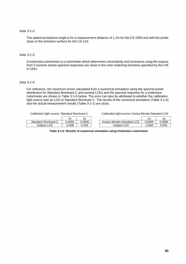
Note 3-1-2:
The stated acceptance angle is for a measurement distance of 1.2m for the CS-1000 and with the probe close to the emission surface for the CA-110.
Note 3-1-3:
A tristimulus colorimeter is a colorimeter which determines chromaticity and luminance using the outputs from 3 sensors whose spectral responses are close to the color-matching functions specified by the CIE in 1931.
Note 3-1-4:
For reference, the maximum errors calculated from a numerical simulation using the spectral power distribution for Standard Illuminant C and several LCDs and the spectral response for a tristimulus colorimeter are shown in Table 3-1-6 below. The error can also be attributed to whether the calibration light source was an LCD or Standard Illuminant C. The results of the numerical simulation (Table 3-1-6) and the actual measurement results (Table 3-1-1) are close.
Calibration light source: Standard Illuminant C Calibration light source: Konica Minolta Standard LCD
∆x ∆y ∆x ∆y Standard Illuminant C 0.0000 -0.0000 Konica Minolta Standard LCD 0.0000 0.0000
Subject LCD -0.008 -0.002 Subject LCD -0.002 0.001
Table 3-1-6: Results of numerical simulation using tristimulus colorimeter
85
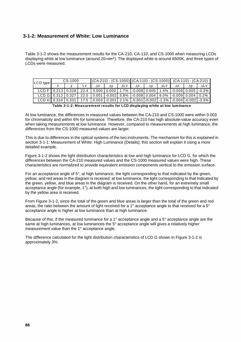
3-1-2: Measurement of White: Low Luminance
Table 3-1-2 shows the measurement results for the CA-210, CA-110, and CS-1000 when measuring LCDs displaying white at low luminance (around 20 ). The displayed white is around 6500K, and three types of LCDs were measured.
x y Lv ∆x ∆y ∆Lv ∆x ∆y ∆Lv ∆x ∆y ∆LvLCD F 0.313 0.328 22.4 0.000 0.000 1.7% -0.008 0.005 1.4% -0.008 0.005 -0.3%LCD G 0.312 0.327 22.0 0.001 -0.002 5.8% -0.008 0.004 6.0% -0.009 0.004 0.2%LCD H 0.310 0.331 17.5 0.003 -0.001 2.1% -0.001 -0.002 -1.3% -0.004 -0.002 -3.3%
(CA-210) - (CS-1000) (CA-110) - (CS-1000) (CA-110) - (CA-210)
Table 3-1-2: Measurement results for LCD displaying white at low luminance
CS-1000LCD type
At low luminance, the differences in measured values between the CA-210 and CS-1000 were within 0.003 for chromaticity and within 6% for luminance. Therefore, the CA-210 has high absolute-value accuracy even when taking measurements at low luminance. However, compared to measurements at high luminance, the differences from the CS-1000 measured values are larger.
This is due to differences in the optical systems of the two instruments. The mechanism for this is explained in section 3-1-1: Measurement of White: High Luminance (Details); this section will explain it using a more detailed example.
Figure 3-1-2 shows the light distribution characteristics at low and high luminance for LCD G, for which the differences between the CA-210 measured values and the CS-1000 measured values were high. These characteristics are normalized to provide equivalent emission components vertical to the emission surface.
For an acceptance angle of 5°, at high luminance, the light corresponding to that indicated by the green, yellow, and red areas in the diagram is received; at low luminance, the light corresponding to that indicated by the green, yellow, and blue areas in the diagram is received. On the other hand, for an extremely small acceptance angle (for example, 1°), at both high and low luminances, the light corresponding to that indicated by the yellow area is received.
From Figure 3-1-2, since the total of the green and blue areas is larger than the total of the green and red areas, the ratio between the amount of light received for a 1° acceptance angle to that received for a 5° acceptance angle is higher at low luminance than at high luminance.
Because of this, if the measured luminance for a 1° acceptance angle and a 5° acceptance angle are the same at high luminances, at low luminances the 5° acceptance angle will gives a relatively higher measurement value than the 1° acceptance angle.
The difference calculated for the light distribution characteristics of LCD G shown in Figure 3-1-2 is approximately 3%.
86

87
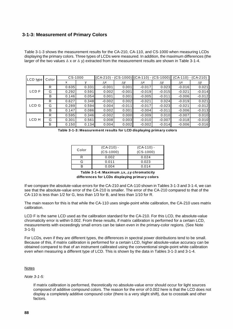
3-1-3: Measurement of Primary Colors
Table 3-1-3 shows the measurement results for the CA-210, CA-110, and CS-1000 when measuring LCDs displaying the primary colors. Three types of LCDs were measured. In addition, the maximum differences (the larger of the two values x or y) extracted from the measurement results are shown in Table 3-1-4.
x y ∆x ∆y ∆x ∆y ∆x ∆yR 0.635 0.331 -0.001 0.001 -0.017 0.023 -0.016 0.021G 0.292 0.591 0.002 -0.001 -0.019 -0.015 -0.021 -0.014B 0.146 0.054 0.001 0.001 -0.005 -0.011 -0.006 -0.012R 0.627 0.348 -0.002 0.002 -0.021 0.024 -0.019 0.021G 0.289 0.594 0.004 -0.011 -0.017 -0.023 -0.021 -0.012B 0.147 0.086 0.002 0.001 -0.004 -0.011 -0.006 -0.013R 0.595 0.346 -0.002 0.000 -0.009 0.010 -0.007 0.010G 0.301 0.561 0.008 0.003 -0.010 -0.007 -0.018 -0.010B 0.150 0.134 0.004 0.002 -0.002 -0.014 -0.006 -0.016
(CA-210) - (CS-1000) (CA-110) - (CS-1000) (CA-110) - (CA-210)
Table 3-1-3: Measurement results for LCD displaying primary colors
Color
LCD F
LCD G
LCD H
CS-1000LCD type
Color(CA-210) - (CS-1000)
(CA-110) - (CS-1000)
R 0.002 0.024G 0.011 0.023B 0.004 0.014
Table 3-1-4: Maximum ∆x, ∆y chromaticity differences for LCDs displaying primary colors
If we compare the absolute-value errors for the CA-210 and CA-110 shown in Tables 3-1-3 and 3-1-4, we can see that the absolute-value error of the CA-210 is smaller. The error of the CA-210 compared to that of the CA-110 is less than 1/2 for G, less than 1/3 for B, and less than 1/10 for R.
The main reason for this is that while the CA-110 uses single-point white calibration, the CA-210 uses matrix calibration.
LCD F is the same LCD used as the calibration standard for the CA-210. For this LCD, the absolute-value chromaticity error is within 0.002. From these results, if matrix calibration is performed for a certain LCD, measurements with exceedingly small errors can be taken even in the primary-color regions. (See Note 3-1-5)
For LCDs, even if they are different types, the differences in spectral power distributions tend to be small. Because of this, if matrix calibration is performed for a certain LCD, higher absolute-value accuracy can be obtained compared to that of an instrument calibrated using the conventional single-point white calibration even when measuring a different type of LCD. This is shown by the data in Tables 3-1-3 and 3-1-4.
Notes
Note 3-1-5:
If matrix calibration is performed, theoretically no absolute-value error should occur for light sources composed of additive compound colors. The reason for the error of 0.002 here is that the LCD does not display a completely additive compound color (there is a very slight shift), due to crosstalk and other factors.
88

3-1-4: Measurement of Intermediate Colors
Table 3-1-5 shows the measurement results for the CA-210, CA-110, and CS-1000 when measuring an LCD displaying white, the primary colors, and intermediate colors.
x y ∆x ∆y ∆x ∆y ∆x ∆yW 0.3132 0.3307 0.0005 0.0002 -0.0072 0.0013 -0.0077 0.0011R 0.6354 0.3305 -0.0015 0.0014 -0.0174 0.0225 -0.0159 0.0211G 0.2919 0.5911 0.0017 -0.0012 -0.0189 -0.0151 -0.0206 -0.0139B 0.1460 0.0540 0.0006 0.0008 -0.0050 -0.0110 -0.0056 -0.0118
Ye (R+G) 0.4203 0.4913 -0.0001 -0.0009 -0.0153 -0.0043 -0.0152 -0.0034Cy (G+B) 0.2191 0.3369 0.0015 -0.0003 -0.0111 -0.0049 -0.0126 -0.0046Mg (B+R) 0.2885 0.1342 0.0000 0.0010 0.0025 0.0058 0.0025 0.0048
(CA-210) - (CS-1000) (CA-110) - (CS-1000) (CA-110) - (CA-210)
Table 3-1-5: Measurement results for LCD displaying primary colors and intermediate colors
Color CS-1000
From the results shown in Table 3-1-5, we can see that the absolute-value error for the CA-210 when measuring intermediate colors is lower than when measuring primary colors. In other words, the error for points within the chromaticity space enclosed by the matrix calibration points is less than the error for the primary colors.
In the same way, the absolute-value error for the CA-110 is smaller for intermediate colors than for primary colors, but this error is larger than that of the CA-210. (See section 3-1-4: Measurement of Intermediate Colors .)
The above results can be understood from Figures 4-1 to 4-4 below. CA-110 is calibrated using single-point white calibration, and as a result, the displayable color chromaticity space is converted linearly from the triangular area in Figure 4-3 to the space in Figure 4-4. In other words, since the difference between the true value and the measured value is a linear relationship, when the calibration point is matched to the true value as in the figure, the errors are the maximum at the corners of the triangle, and the error is smaller for intermediate colors than for primary colors (which are at each of the corners of the triangle).
For matrix calibration, after performing RGB calibration, the displayable color chromaticity space is converted linearly from the triangular area in Figure 4-1 to the space in Figure 4-2, and any measured point within the displayable color chromaticity space will be the true value. However, CA series instruments use the method of single-point white calibration applied to the R, G, B matrix coefficients (see section 1-4-1: Matrix Calibration Overview) to take into account the slight shifts from additive compound colors which occur with LCDs. As a result of this, just like for single-point white calibration, the errors are the maximum at the corners of the triangle, and the error is smaller for intermediate colors than for primary colors (which are at each of the corners of the triangle).
89

90

3-2: Gamma Characteristics Comparison
3-2-1: Comparison of Gamma Characteristics Measurements
• References to CA-210 measurements in the following refer to measurements with the CA-210 LCD Flicker Measuring Probe.
Figure 3-2-1 and Table 3-2-1 show the gamma characteristics of an LCD measured using the CA-110, CA-210, and CS-1000. (See Note 3-2-1.)
For each color R, G, and B, it can be seen that the CA-210 measurement results are close to those of the CS-1000.On the other hand, the curve for the CA-110 is more gentle than those for the CA-210 or CS-1000.
The reason for the differences in the γ characteristics measured by the CA-110, CA-210, and CS-1000 are differences in the optical systems of each instrument. This section will explain those differences.
91

Figure 3-2-2 shows the light distribution characteristics of LCDs at low and high luminance. These characteristics are normalized to provide equivalent emission components vertical to the emission surface.
92
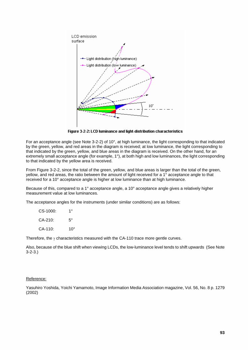
For an acceptance angle (see Note 3-2-2) of 10°, at high luminance, the light corresponding to that indicated by the green, yellow, and red areas in the diagram is received; at low luminance, the light corresponding to that indicated by the green, yellow, and blue areas in the diagram is received. On the other hand, for an extremely small acceptance angle (for example, 1°), at both high and low luminances, the light corresponding to that indicated by the yellow area is received.
From Figure 3-2-2, since the total of the green, yellow, and blue areas is larger than the total of the green, yellow, and red areas, the ratio between the amount of light received for a 1° acceptance angle to that received for a 10° acceptance angle is higher at low luminance than at high luminance.
Because of this, compared to a 1° acceptance angle, a 10° acceptance angle gives a relatively higher measurement value at low luminances.
The acceptance angles for the instruments (under similar conditions) are as follows:
CS-1000: 1°
CA-210: 5°
CA-110: 10°
Therefore, the γ characteristics measured with the CA-110 trace more gentle curves.
Also, because of the blue shift when viewing LCDs, the low-luminance level tends to shift upwards (See Note 3-2-3.)
Reference:
Yasuhiro Yoshida, Yoichi Yamamoto, Image Information Media Association magazine, Vol. 56, No. 8 p. 1279 (2002)
93

Notes:
Note 3-2-1:
The relationship between the image signal input to the display and the emitted luminance can be expressed as follows:
γinout VAV •=
Where:
Vout = Emitted luminance
Vin = Input image signal
A = Constant
This relationship is termed " γ characteristics".
Note 3-2-2:
Acceptance angle is the angle at the surface of the measurement subject of the range of light rays accepted by the measuring instrument.
Note 3:
Light from LCDs include leaked light, and the amount of leaked light included is greater at longer wavelengths than at shorter ones. This phenomenon is clearly revealed at low luminance levels, where the displayed color is noticeably bluer. This is termed "Blue shift".
In these measurement examples, the X value is used to determine the R γ characteristics, the Y value is used to determine the G γ characteristics, and the Z value is used to determine the B γ characteristics (conforming to the evaluation method specified in IEC-61966). Since the X and Y sensors have low sensitivity to short wavelengths, they are not affected much by the blue shift, but since the Z sensor has high sensitivity at short wavelengths, it is affected by the blue shift. Therefore, the measurement values for the R and G γ characteristics are not affected by the blue shift, and only the measurement values for the B γ characteristics are affected.
94

3-3: LCD Measurement Differences for CA-210 LCD Flicker Measuring Probes and CS-1000 3-3-1: Measurements of White
Tables 3-3-1 and 3-3-2 show the measurement results for LCDs displaying white at high luminance (100 or higher) and at low luminance (around 20 ) respectively for measurements taken with the CA-210 Small LCD Flicker Measuring Probe (hereafter referred to as CA-210S), CA-210 LCD Flicker Measuring Probe (hereafter referred to as CA-210), and the CS-1000. The displayed white is around 6500K and three types of LCDs were measured.
x y Lv ∆x ∆y ∆Lv ∆x ∆y ∆Lv ∆x ∆y ∆LvLCD L 0.313 0.329 155.0 0.000 0.000 0.1% 0.000 0.000 0.0% 0.000 0.000 -0.1%LCD M 0.315 0.333 156.8 -0.001 -0.001 0.4% -0.001 -0.001 -2.3% 0.000 0.001 -2.6%LCD N 0.313 0.330 99.1 0.001 -0.001 -1.2% 0.001 -0.001 -1.2% 0.000 0.000 -0.1%
(CA-210S) - (CS-1000) (CA-210) - (CS-1000) (CA-210) - (CA-210S)
Table 3-3-1: Measurement results for LCD displaying white at high luminance
CS-1000LCD type
x y Lv ∆x ∆y ∆Lv ∆x ∆y ∆Lv ∆x ∆y ∆LvLCD L 0.311 0.328 20.1 0.000 0.001 2.8% 0.000 0.000 0.1% 0.000 -0.001 -2.6%LCD M 0.314 0.328 20.4 -0.002 0.000 -0.1% -0.001 0.000 0.3% 0.001 0.000 0.4%LCD N 0.312 0.329 20.5 0.001 0.000 -0.2% 0.001 0.000 0.3% 0.000 0.000 0.5%
(CA-210S) - (CS-1000) (CA-210) - (CS-1000) (CA-210) - (CA-210S)
Table 3-3-2: M easure m ent results for LCD displaying w hite at low lum inance
CS-1000LCD type
If we consider the values measured by the Spectroradiometer CS-1000 as the true values, then the differences between those values and the values measured by the CA-210S and CA-210 can be considered as the absolute-value errors for the respective instruments.
The differences in measured values between the CA-210S/CA-210 and CS-1000 were within 0.002 for chromaticity and within 3% for luminance. Therefore, from this data it can be said that the CA-210S and CA-210 have high absolute-value accuracy even when measuring different types of LCDs. (See section 1-2: About Color-Measuring Instruments.)
In addition, the difference between the CA-210S and the CA-210 is within 0.001 for chromaticity and within 3% for luminance. Table 3-3-3 shows the differences between the acceptance angles and measuring areas of the CA-210S and CA-210, but these do not seem to cause major differences for measurements of LCDs displaying white.
CA-210S CA-210Acceptance angle (deg) 10 5Measurem ent area (Øm m ) 10 27
Table 3-3-3: Comparison of CA-210S and CA-210 specifications
95

3-3-2: Measurements of Primary Colors
Table 3-3-4 shows the measurement results for the CA-210S, CA-210, and CS-1000 when measuring LCDs displaying the primary colors. Three types of LCDs were measured.
x y ∆x ∆y ∆x ∆y ∆x ∆yR 0.634 0.331 0.001 -0.001 0.001 0.000 -0.001 0.001G 0.293 0.591 0.001 -0.001 0.000 0.000 -0.001 0.001B 0.146 0.055 0.000 0.000 0.000 0.000 0.000 0.000R 0.626 0.349 0.000 -0.001 0.000 0.000 -0.001 0.001G 0.289 0.594 0.000 -0.007 0.000 -0.007 0.000 0.000B 0.147 0.087 0.002 0.002 0.002 0.001 0.000 -0.001R 0.596 0.346 -0.001 -0.001 0.002 -0.004 0.003 -0.002G 0.302 0.561 0.003 0.008 0.003 0.010 0.000 0.002B 0.150 0.136 0.003 0.002 0.003 0.003 -0.001 0.001
(CA-210S) - (CS-1000) (CA-210) - (CS-1000) (CA-210) - (CA-210S)
Table 3-3-4: Measurement results for LCD displaying primary colors
Color
LCD L
LCD M
LCD N
CS-1000LCD type
The differences between the CS-1000 and both the CA-210S and CA-210 were within 0.010 for chromaticity. Compared to the 0.020 to 0.030 primary-color accuracy for conventional tristimulus colorimeters, this is clearly a great improvement in accuracy. This is due to the matrix calibration used for the CA-210S and CA-210. (See section 1-4-1: Matrix Calibration Overview.)
In addition, the difference between the CA-210S and the CA-210 is a maximum of 0.003 for chromaticity. This is somewhat larger than the difference for white. The CA-210S and CA-210 use single-point white calibration applied to the R, G, B matrix coefficients, which gives an accuracy of ±0.002 for white but a somewhat worse accuracy of ±0.004 for primary colors. (See section 1-4-1: Matrix Calibration Overview.) This is the reason for the above differences.
96

3-4: Flicker Measurement Accuracy
3-4-1: Flicker Measurement Accuracy: Contrast Method
The specifications for flicker measurement (Contrast Method) accuracy and repeatability are defined as follows for the given conditions:
Value: Conditions:± 1% 30Hz (AC/DC 10% sine w ave)± 2% 60Hz (AC/DC 10% sine w ave)
Value: Conditions:Repeatability: 1% 20 to 65Hz (AC/DC 10% sine w ave)
Accuracy:
(See Note 3-4-1.)
For conditions other than those stated above, an evaluation jig was used to take actual measurements, and the flicker measurement (Contrast Method) accuracy and repeatability were evaluated. The results of such evaluation are shown in Tables 3-4-1 and 3-4-2 below. (See section 2-2: Definition of Flicker Accuracy Standards and Repeatability.) (See Note 3-4-2.) Note that the frequency listed below is the frequency input to the measuring instrument. The emission frequency when flicker occurs is 1/2 the vertical synchronization frequency of the display. (See section 1-7-1: What is LCD Flicker?)
5cd/m 2 (Units: %) 70cd/m 2 (Units: %)True value 20Hz 30Hz 40Hz 50Hz 58Hz
True value 20Hz 30Hz 40Hz 50Hz 58Hz
5.7 0.1 0.0 -0.1 0.2 0.0 5.8 -0.1 -0.1 0.0 0.1 -0.110.0 0.0 0.0 0.0 0.1 -0.1 10.0 0.0 -0.1 -0.4 0.0 0.120.0 0.3 0.0 0.0 0.3 -0.3 19.8 -0.2 -0.1 -0.2 -0.1 0.340.0 0.4 0.3 0.2 0.5 -0.6 39.5 -0.2 -0.2 -0.4 -0.1 0.880.0 1.0 0.6 -0.2 0.6 -1.2 79.1 -0.3 -0.6 -1.0 -0.3 1.3
Table 3-4-1: Flicker m easurem ent (Contras t M ethod) accuracy e rror for various lum inances and freque ncies
5cd/m 2 (Units: %) 70cd/m 2 (Units: %)True value 20Hz 30Hz 40Hz 50Hz 58Hz
True value 20Hz 30Hz 40Hz 50Hz 58Hz
5.7 0.3 0.2 0.2 0.1 0.2 5.8 0.0 0.0 0.0 0.0 0.010.0 0.1 0.1 0.2 0.3 0.4 10.0 0.3 0.1 0.1 0.1 0.120.0 0.2 0.2 0.2 0.1 0.2 19.8 0.2 0.1 0.1 0.1 0.140.0 0.2 0.2 0.2 0.1 0.2 39.5 0.3 0.1 0.1 0.1 0.280.0 0.1 0.2 0.2 0.2 0.2 79.1 0.4 0.0 0.2 0.0 0.1
Table 3-4-2: Flick er m easurem ent (Contras t M ethod) re peatability for various lum inances and frequencies
From the results shown in Tables 3-4-1 and 3-4-2, the following can be stated:
Measurement accuracy error:
• Is affected by the amount of flicker. As the flicker value increases, the measurement accuracy error also increases. (However, for all conditions, the measurement accuracy error is within 1/10 of the flicker value.
97
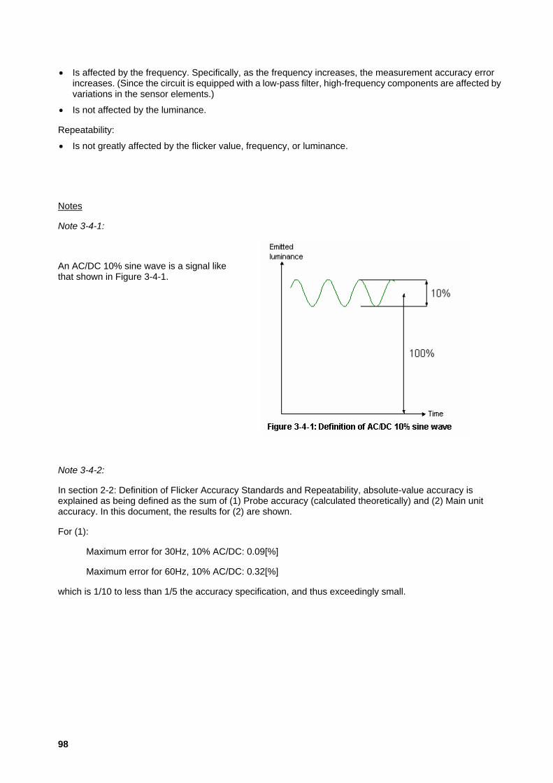
• Is affected by the frequency. Specifically, as the frequency increases, the measurement accuracy error increases. (Since the circuit is equipped with a low-pass filter, high-frequency components are affected by variations in the sensor elements.)
• Is not affected by the luminance.
Repeatability:
• Is not greatly affected by the flicker value, frequency, or luminance.
Notes
Note 3-4-1:
An AC/DC 10% sine wave is a signal like that shown in Figure 3-4-1.
Note 3-4-2:
In section 2-2: Definition of Flicker Accuracy Standards and Repeatability, absolute-value accuracy is explained as being defined as the sum of (1) Probe accuracy (calculated theoretically) and (2) Main unit accuracy. In this document, the results for (2) are shown.
For (1):
Maximum error for 30Hz, 10% AC/DC: 0.09[%]
Maximum error for 60Hz, 10% AC/DC: 0.32[%]
which is 1/10 to less than 1/5 the accuracy specification, and thus exceedingly small.
98

3-4-2: Flicker Measurement Accuracy: JEITA Method
The specifications for flicker measurement (JEITA Method) accuracy and repeatability are defined as follows for the given conditions:
Value: Conditions:Accuracy: ± 0.5dB 30Hz (AC/DC 10% sine w ave)
Value: Conditions:Repeatability: 0.3dB 30Hz (AC/DC 10% sine w ave)
(See Note 3-4-1.)
For conditions other than those stated above, an evaluation jig was used to take actual measurements, and the flicker measurement (JEITA Method) accuracy and repeatability were evaluated. The results of such evaluation are shown in Tables 3-4-3 to 3-4-5 below. (See section 2-2: Definition of Flicker Accuracy Standards and Repeatability.) (See Note 3-4-3.)
5cd/m 2 (Units: dB) 70cd/m 2 (Units: dB)AC/DC
ratio(%)
20Hz 30Hz 40Hz 50Hz 58HzAC/DC
ratio(%)
20Hz 30Hz 40Hz 50Hz 58Hz
5.7 -33.97 -37.06 -40.18 -46.34 -61.23 5.8 -33.85 -36.94 -40.07 -46.23 -61.1210.0 -29.11 -32.20 -35.32 -41.48 -56.37 10.0 -29.11 -32.20 -35.32 -41.48 -56.3720.0 -23.09 -26.18 -29.30 -35.46 -50.35 21.1 -22.64 -25.73 -28.86 -35.01 -49.9040.0 -17.06 -20.16 -23.28 -29.44 -44.33 39.5 -17.18 -20.27 -23.40 -29.55 -44.4480.0 -11.04 -14.14 -17.26 -23.42 -38.31 78.9 -11.16 -14.25 -17.38 -23.53 -38.42
Table 3-4-3: True m e as ured flick er values (JEITA M ethod) for various lum inances and frequencies
(For information regarding AC/DC ratio, see Note 3-4-1.)
5cd/m 2 (Units: dB) 70cd/m 2 (Units: dB)AC/DC
ratio(%)
20Hz 30Hz 40Hz 50Hz 58HzAC/DC
ratio(%)
20Hz 30Hz 40Hz 50Hz 58Hz
5.7 0.13 0.28 0.47 0.74 1.17 5.8 0.10 0.24 0.44 0.71 1.1410.0 0.11 0.25 0.45 0.72 1.15 10.0 0.08 0.23 0.42 0.69 1.1220.0 0.11 0.26 0.45 0.72 1.15 21.1 0.18 0.32 0.52 0.80 1.2240.0 0.11 0.26 0.45 0.73 1.16 39.5 0.17 0.31 0.51 0.79 1.2180.0 0.10 0.25 0.44 0.72 1.15 78.9 0.16 0.31 0.51 0.78 1.21
Table 3-4-4: Flick er m easure m ent (JEITA M ethod) accuracy e rror for various lum inances and frequencies
(For information regarding AC/DC ratio, see Note 3-4-1.)
99

5cd/m 2 (Units: dB) 70cd/m 2 (Units: dB)AC/DC
ratio(%)
20Hz 30Hz 40Hz 50Hz 58HzAC/DC
ratio(%)
20Hz 30Hz 40Hz 50Hz 58Hz
5.7 0.01 0.01 0.02 0.01 0.01 5.8 0.01 0.01 0.01 0.01 0.0110.0 0.01 0.01 0.01 0.01 0.01 10.0 0.01 0.01 0.01 0.01 0.0020.0 0.00 0.00 0.00 0.01 0.01 21.1 0.00 0.00 0.00 0.00 0.0040.0 0.00 0.00 0.00 0.00 0.00 39.5 0.00 0.00 0.00 0.00 0.0080.0 0.01 0.00 0.00 0.00 0.00 78.9 0.00 0.00 0.00 0.00 0.00
Table 3-4-5: Flicke r m e as ure m ent (JEITA M ethod) repeatability for various lum inances and frequencies
(For information regarding AC/DC ratio, see Note 3-4-1.)
From the results shown in Tables 3-4-3 to 3-4-5, the following can be stated:
Measurement accuracy error:
• Is not affected by the amount of flicker.
• Is affected by the frequency. Specifically, as the frequency increases, the measurement accuracy error increases. (Since the circuit is equipped with a low-pass filter, high-frequency components are affected by variations in the sensor elements.)
• Is not affected by the luminance.
Repeatability:
• Is not greatly affected by the flicker value, frequency, or luminance.
Note that when a signal with a frequency of 30Hz is input to the CA-210 main body, frequency components at frequencies other than 30Hz are less than -80[dB] (when the equations used in the flicker definition are applied to each frequency component). This is equivalent to an AC/DC ratio of 0.1% or less.
Notes
Note 3-4-1:
An AC/DC 10% sine wave is a signal like that shown in Figure 3-4-1.
100

Note 3-4-3:
In section 2-2: Definition of Flicker Accuracy Standards and Repeatability, absolute-value accuracy is explained as being defined as the sum of (1) Probe accuracy (calculated theoretically) and (2) Main unit accuracy. In this document, the results for (2) are shown.
For (1):
Maximum error for 30Hz, 10% AC/DC: 0.08[dB]
which is less than 1/5 the accuracy specification, and thus exceedingly small.
101

3-5: Measurement Speed
3-5: Measurement Speed (Detailed Explanation)
Comparison of speed when one probe is connected and when 5 probes are connected
The measurement speed of the CA-210 depends on the following measurement modes and conditions:
Measurement speed mode: FAST, SLOW
Measurement mode: xyLv, T∆uvLv, Flicker, etc.
Measurement sync mode: NTSC, PAL, etc.
Number of probes: 1 to 5
Type of interface used: (USB, RS-232C)
Tables 3-5-1 through 3-5-3 show the measurement speeds under the various condition combinations.
xyLvFlicker
(Contrast method) xyLvFlicker
(Contrast method)NTSC 20 16 13 7PAL 17 14 11 6
EXT (60Hz) 20 16 13 7UNIV 8 (Note 1) 6 (Note 1)
INT (60Hz) 20 16 13 7NTSC 5 (Note 2) 3.5 (Note 2)PAL 4 (Note 2) 3 (Note 2)
EXT (60Hz) 5 (Note 2) 3.5 (Note 2)UNIV 1.5 (Note 2) 1.5 (Note 2)
INT (60Hz) 5 (Note 2) 3.5 (Note 2)
FAST
SLOW
Table 3-5-1: Re lationship be tw een m easurem ent speed and m easurem ent speed m ode /m easurem ent sync m ode for USB connection
(Units: Measurements/sec.)When 1 probe connected When 5 probes connected
Measurementspeed mode
Measurementsync mode
102

xyLvFlicker
(Contrast method) xyLvFlicker
(Contrast method)NTSC 17 16 7 6PAL 15 14 6 5
EXT (60Hz) 17 16 7 6UNIV 7 (Note 1) 4 (Note 1)
INT (60Hz) 17 16 7 6NTSC 4.5 (Note 2) 3 (Note 2)PAL 4 (Note 2) 2.5 (Note 2)
EXT (60Hz) 4.5 (Note 2) 3 (Note 2)UNIV 1.5 (Note 2) 1 (Note 2)
INT (60Hz) 4.5 (Note 2) 3 (Note 2)
FAST
SLOW
Table 3-5-2: Re lationship be tw een m easurem ent speed and m easurem ent speed m ode /m easurem ent sync m ode for RS-232C connection
(Units: Measurements/sec.)When 1 probe connected When 5 probes connected
Measurementspeed mode
Measurementsync mode
USB RS-232C USB RS-232C
xyLv 20 17 13 7u'v 'Lv 19 17 12 6
Analyzer 20 17 13 7XYZ 20 17 13 7T∆ uv 19 17 12 5.5
Flicker (Contrast method)
16 16 7 6
NTSCFAST
Table 3-5-3: Re lationship be tw een m easurem ent s peed and m easurem ent m ode
(Units: Measurements/sec.)
When 1 probe connected When 5 probes connectedMeasurement speed mode
Measurement sync mode
Measurementmode
Note 1: Invalid setting
Note 2: Flicker measurements possible in FAST mode only. (SLOW mode cannot be set.)
Evaluation conditions:
PC: Pentium II (300MHz)
OS: Windows 2000, Windows 98, Windows Me
RS-232C baud rate: 38,400bps
103

3-6: CRT Measurement Differences for CA-100 and CA-100Plus
3-6-1: Measurements of White
The results for measurements of 4 CRT models displaying white (color temperature: approximately 6500K) at various luminance levels taken with the CA-100Plus and CA-100 are shown in Table 3-6-1.
x y Lv x y Lv ∆x ∆y ∆LvCRT 1 0.314 0.330 39.5 0.313 0.329 39.7 -0.001 -0.001 0.5%CRT 2 0.314 0.329 74.6 0.312 0.328 74.4 -0.002 -0.001 -0.3%CRT 3 0.314 0.330 86.8 0.313 0.329 87.0 -0.001 -0.001 0.2%CRT 4 0.315 0.329 70.8 0.313 0.329 70.8 -0.002 0.000 0.0%
CA-100Plus CA-100 (CA-100) - (CA-100Plus )
Table 3-6-1: Measurement results for CRT displaying white at high luminance
The differences between the CA-100Plus and CA-100 when measuring white are within a maximum of 0.002 for chromaticity and 0.5% for luminance, which are within the accuracy specifications for the CA-100Plus and CA-100.
104

3-6-2: Measurements of Primary Colors
After setting 4 CRT models to display white (color temperature: approximately 6500K) at various luminance levels, the CRTs were set to display the primary colors and measurements were taken with the CA-100Plus and CA-100. The results of these measurements are shown in Table 3-6-2.
x y Lv x y Lv ∆x ∆y ∆LvR 0.626 0.340 9.8 0.634 0.333 10.0 0.008 -0.007 2.5%G 0.288 0.607 27.5 0.278 0.607 27.9 -0.010 0.000 1.5%B 0.153 0.069 3.4 0.142 0.062 3.0 -0.011 -0.007 -12.5%R 0.605 0.342 19.1 0.612 0.336 19.3 0.007 -0.006 1.0%G 0.292 0.588 50.7 0.283 0.587 51.0 -0.009 -0.001 0.6%B 0.161 0.087 8.0 0.151 0.080 7.1 -0.010 -0.007 -10.8%R 0.633 0.328 24.3 0.641 0.322 24.9 0.008 -0.006 2.5%G 0.285 0.597 76.2 0.275 0.596 77.2 -0.010 -0.001 1.3%B 0.155 0.071 9.5 0.144 0.065 8.5 -0.011 -0.006 -11.0%R 0.630 0.335 15.7 0.637 0.329 16.1 0.007 -0.006 2.5%G 0.299 0.605 46.9 0.289 0.604 47.5 -0.010 -0.001 1.3%B 0.154 0.072 6.0 0.143 0.065 5.3 -0.011 -0.007 -11.7%
Table 3-6-2: CA-100Plus and CA-100 measurement results for CRTs displaying primary colors
Color
CRT 1
CRT 3
CRT 4
CA-100Plus CA-100 (CA-100)-(CA-100Plus )
CRT 2
Since the luminances of the 4 CRTs were set to different levels as shown in Table 1-1 when they were displaying white, their luminance levels when displaying the primary colors were also different.
The values measured with the CA-100Plus had maximum differences of around 0.011 for chromaticity and 12% for luminance. The maximum differences for both values occurred for measurements of B.
The reason for these differences in the B values is the difference in calibration methods.
The CA-100 is calibrated using single-point white calibration, while the CA-100Plus is calibrated using WRGB matrix calibration (single-point white calibration applied to the R, G, B matrix coefficients). (Refer to 1-4-1: Matrix Calibration Overview.)
This would be explained as follows:
As shown in Figure 3-6-1b, WRGB matrix calibration of the CA-100Plus provides measurements of both white and primary colors which are almost the same as the true values. With the CA-100, although single-point white calibration provides measurements of white which are almost the same as the true values, since calibration is not performed for the primary colors, measurements of the primary colors are shifted from their true values.
In Figures 3-6-1a and 3-6-1c, although the errors between the true values and measured values before calibration for the CA-100 and CA-100Plus are different, this is due to variances in the spectral sensitivities of the two instruments. For tristimulus colorimeters, differences in spectral sensitivities result in larger errors for the primary colors which cannot be reduced by single-point white calibration.
Table 3-6-3 shows the maximum errors for numerical simulation of measurements of primary colors on 21 CRT models using the two calibration methods, taking into consideration the differences in spectral sensitivities. For single-point white calibration, the error for chromaticity is extremely large at 0.027, but for matrix calibration the error for chromaticity is smaller by one decimal place, at 0.0016.
105

∆x ∆y ∆Lv (%) ∆x ∆y ∆Lv (%)Absolute-value error 0.027 0.021 14.8 0.002 0.002 1.6
Table 3-6-3: Results of numerical simulation of absolute-value error (maximum) for CRT displaying primary colors
Single-point white calibration Matrix calibration
In other words, while the CA-100Plus has data compatibility with the CA-100, it provides greatly improved chromaticity accuracy for primary colors.
106

107

3-7: CA-100Plus and CA-100 Measurement Error for CRTs and PDPs
3-7-1: Measurement of White at High Luminance (CRT)
In order to provide data compatibility between the CA-100Plus and the CA-100, sensors with the same spectral response are used and both instruments are calibrated to CRTs having the same spectral emission characteristics.
The results for measurements of CRTs displaying white at high luminance taken with the two instruments (CA-100Plus and CA-100) are shown in Table 3-7-1. The white was approximately 6500K, and four CRT models were measured. (CRT 1 is the calibration CRT for the CA-100Plus.)
x y Lv x y Lv ∆x ∆y ∆LvCRT 1 0.314 0.330 39.5 0.313 0.329 39.7 -0.001 -0.001 0.5%CRT 2 0.314 0.329 74.6 0.312 0.328 74.4 -0.002 -0.001 -0.3%CRT 3 0.314 0.330 86.8 0.313 0.329 87.0 -0.001 -0.001 0.2%CRT4 0.315 0.329 70.8 0.313 0.329 70.8 -0.002 0.000 0.0%
CA-100Plus CA-100 (CA-100) - (CA-100Plus )
Table 3-7-1: Measurement results for CRT displaying white at high luminance
The differences between the two instruments are within 0.002 for chromaticity and 0.5% for luminance, which are within the accuracy specifications (±0.002 for chromaticity; ±2% for luminance) for the CA-100Plus and CA-100.
As stated before, the CA-100Plus is calibrated to a CRT with the same spectral emission characteristics as the one used for calibrating the CA-100, and also the sensor spectral sensitivities of the two instruments are the same, so that data measured with the two instruments can be said to be compatible.
108

3-7-2: Measurement of White at Low Luminance (CRT)
The results for measurements of CRTs displaying white at low luminance taken with the two instruments (CA-100Plus and CA-100) are shown in Table 3-7-2. Four CRT models were measured. (CRT 1 is the calibration CRT for the CA-100Plus.)
x y Lv x y Lv ∆x ∆y ∆LvCRT 1 0.314 0.329 4.9 0.312 0.329 4.9 -0.002 0.000 0.8%CRT 2 0.312 0.329 5.3 0.314 0.329 5.3 0.002 0.000 0.0%CRT 3 0.314 0.329 5.0 0.313 0.329 5.0 -0.001 0.000 -0.8%CRT 4 0.314 0.330 5.0 0.312 0.330 5.1 -0.002 0.000 1.0%
CA-100Plus CA-100 (CA-100) - (CA-100Plus )
Table 3-7-2: Measurement results for CRT displaying white at low luminance
In this case also, the differences between the two instruments are within 0.002 for chromaticity and 1% for luminance, which are within the accuracy specifications for the CA-100Plus and CA-100.
Even for measurements at low luminance, data measured with the CA-100Plus can be said to be compatible with those measured with the CA-100.
109
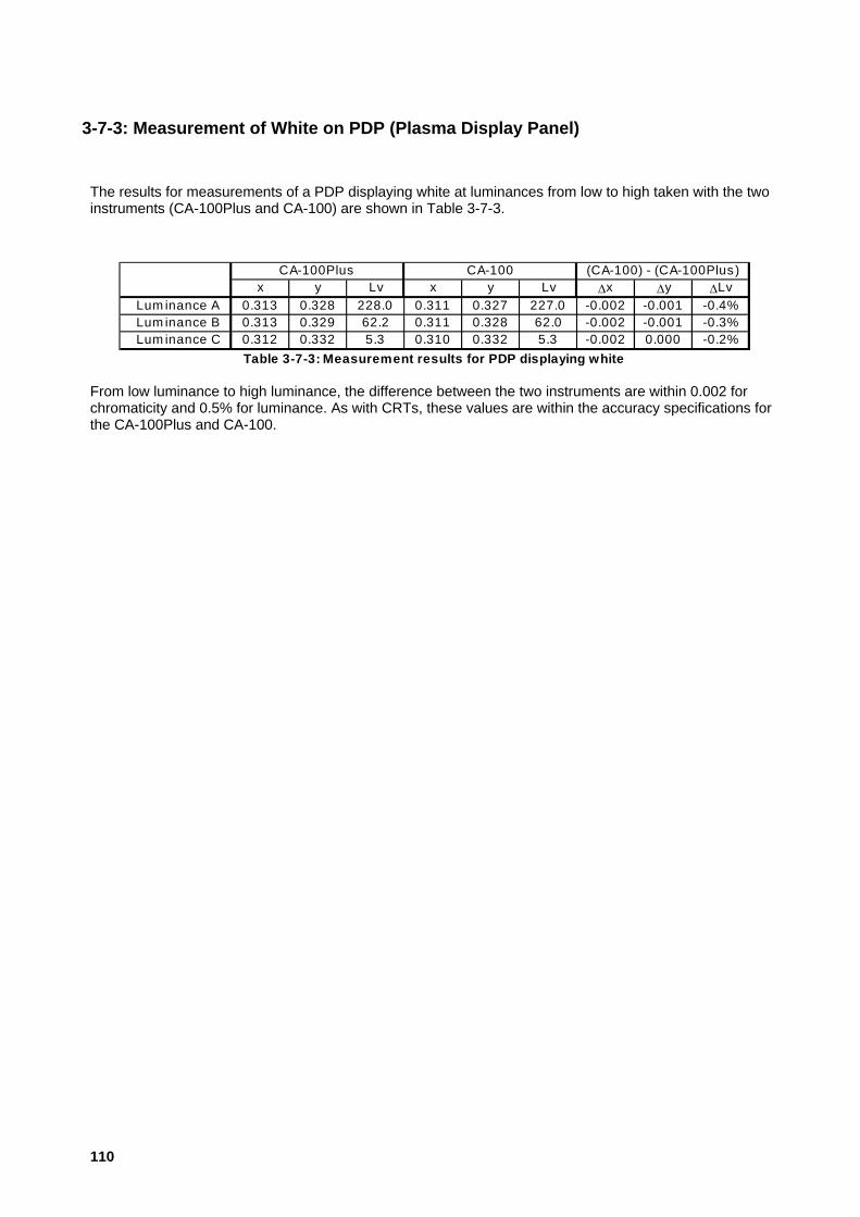
3-7-3: Measurement of White on PDP (Plasma Display Panel)
The results for measurements of a PDP displaying white at luminances from low to high taken with the two instruments (CA-100Plus and CA-100) are shown in Table 3-7-3.
x y Lv x y Lv ∆x ∆y ∆LvLum inance A 0.313 0.328 228.0 0.311 0.327 227.0 -0.002 -0.001 -0.4%Lum inance B 0.313 0.329 62.2 0.311 0.328 62.0 -0.002 -0.001 -0.3%Lum inance C 0.312 0.332 5.3 0.310 0.332 5.3 -0.002 0.000 -0.2%
CA-100Plus CA-100 (CA-100) - (CA-100Plus)
Table 3-7-3: Measurement results for PDP displaying white
From low luminance to high luminance, the difference between the two instruments are within 0.002 for chromaticity and 0.5% for luminance. As with CRTs, these values are within the accuracy specifications for the CA-100Plus and CA-100.
110
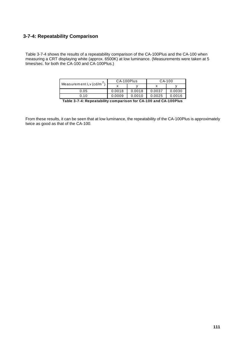
3-7-4: Repeatability Comparison
Table 3-7-4 shows the results of a repeatability comparison of the CA-100Plus and the CA-100 when measuring a CRT displaying white (approx. 6500K) at low luminance. (Measurements were taken at 5 times/sec. for both the CA-100 and CA-100Plus.)
x y x y0.05 0.0018 0.0018 0.0037 0.00300.10 0.0009 0.0010 0.0025 0.0016
CA-100Plus CA-100
Table 3-7-4: Repeatability comparison for CA-100 and CA-100Plus
Measurem ent Lv (cd/m 2)
From these results, it can be seen that at low luminance, the repeatability of the CA-100Plus is approximately twice as good as that of the CA-100.
111

4: CA-SDK Software Explanation 4-1: What is COM?
4-1: Introduction
This section will provide an overview of the COM technology necessary for creating applications in Visual C/C++ (hereafter referred to as VC++; Not) using the CA-SDK.
• The CA-SDK is compatible only with 32-bit mode applications. When creating applications using the CA-SDK, be sure to set 32-bit mode.
112
4-1-1: COM Interface
4-1-1-1: Interface
Object-oriented technology is becoming increasingly popular for software development. Object-oriented technology is recognized as a method for efficient development of high-quality software. However, in the explanation of object-oriented technology, it is often stated that the best way to develop software is to not write software at all. By using an object-oriented language such as VC++ and programming by skillfully extracting the features of an object, it becomes possible to achieve modularization and reusability of software -- a longtime dream in the software world.
So how is programming done skillfully? One of the technologies which is emphasized in regard to this point is "interface programming". In order to develop software without writing new software, it is necessary to properly define the functions of the standard components and the interface for combining/using them to enable programming by combining such standard components. The actual software would then be constructed in a building-block fashion, plugging in existing interfaced components which fulfill the standard component specifications and which have been fully tested.
The word "interface" has a variety of meanings, but when used in relation to COM, it has the meaning outlined above. The "class" which has a central role in object-oriented programming, defines the outline for implementation in COM, and in interface programming, it is necessary to program so as to make the class invisible. COM is a programming method which is built upon the concept of thorough interface programming, in which the interface is everything.
Further, "modularization" and "reuseability" as used in object-oriented programming languages such as VC++ typically applies to the source code itself. Because of this, it depends on the language and tools used to develop it. COM, on the other hand, defines the binary structure and memory structures for implementing the interface in the specifications, and aims to implement the interface independent of the development language, tools, or platform. If the interface binary processing which meets the COM specifications can be performed, and the object can be packaged as a binary-level .DLL or .EXE file, enabling modularization and reuse independent of language.
113

4-1-1-2: COM Interface
The definition of the COM interface is an .IDL (.ODL) file separate from the C++ file which implements the interface. When using the COM support functions of MFC to create a COM (automation) server, the tool will create the .ODL file automatically. In addition, when a class for implementing the interface is inserted into the project, the corresponding interface definition will be inserted automatically in the .ODL file. Therefore, normally, it's not necessary to write an interface definition file directly. However, since the C++ sample program in the CA-SDK is an event-driven program (the COM interface will be defined at the application side), modification of part of the .ODL file will be necessary. This section will explain briefly about the COM interface definition (file). As explained in section 4-1-1-1: Interface, in COM the interface is everything. If the interface is defined, the client or server for the interface can be implemented.
When creating software using the CA-SDK, first, it is necessary to set or add the reference to the CA-SDK component. The source code listing below is the code for the structure (called a "type library") which is inserted into the project by performing this process. This is the interface definition.
In the source code listing:
The section after the "library" statement (1) is the section which will be affected by the type library. First, the Ca200 COM class (2) is declared as a class which implements the ICa200 COM interface. The definition for the ICa200 COM interface is then listed from (4) onwards.
From (5), the Cas property of the ICas COM interface is declared.
From (6), the method SetConfiguration and its 4 arguments of type long, BSTR, long, and long are declared.
From (7), the method AutoConnect (which has no arguments) is declared.
From (8), the SingleCa property of the ICa COM interface is declared.
In addition, one other piece of information necessary for creating a client/server program is provided: the GUID (globally unique ID) value. In the code listing, the CLSID (class ID; the ID inside the parentheses of the "uuid ()" statement) of the Ca200 COM class is listed above the class definition (2), and the IID (interface ID) of the ICa200 COM interface is listed above the interface definition.
Except for in the case of automation (which will be explained later), the names in the interface definition have meanings only inside the source program. In the compiled executable (file), the ID values described above are used for identification and processing.
In this way, all the information necessary for interface programming is provided in the type library. Development tools which support COM use this information in various ways to create C++ files for developers (see section 4-2: Creating a VC++ application using the CA-SDK and 4-3: CA-SDK Sample Software Control Methods for examples). If programming must be done without using the tool's support for some reason, the minimum necessary C files for development can be created by passing this file through the MIDL compiler.
// Generated .IDL file (by the OLE/COM Object Viewer)
//
// typelib filename: CA200Srvr.dll
…
library CA200SRVRLib
114

{
[
uuid(006B0650-AF9A-4EE1-B18F-B5740004D7CE),
…
]
coclass Ca200 {
[default] interface ICa200;
};
[
…
uuid(DB87A8F6-FAF3-433A-B7F3-31BB4D759361),
…
]
interface ICa200 : IDispatch {
[…, propget, …]
HRESULT Cas([out, retval] ICas** CasVal);
…
HRESULT SetConfiguration(
[in] long CaNumberVal,
[in] BSTR ConnecStringVal,
[in] long PortVal,
[in, optional, defaultvalue(38400)] long BaudRateVal);
…
HRESULT AutoConnect();
[…, propget, …]
HRESULT SingleCa([out, retval] ICa** SingleCaVal);
};
115

4-1-1-3: COM Interface Programming
In the client software which will use the COM component, the following sequence of processes must be performed:
1 Instantiate a COM object with the interface to a COM class which implements and makes public the required COM interface and obtain the IUnknown interface
2 Obtain the required COM interface from IUnknown.
3 Perform the processes required by the client using the obtained COM interface.
4 Release the interface when it is no longer necessary.
In this explanation, the IUnknown interface was not present in the definition shown in section 4-1-1-2: COM Interface .
The CA-SDK is defined as having a so-called dual interface (an interface with combined automation functions). In the definition of the ICa200 COM interface (4) in the code listing of section 4-1-1-2: COM Interface, ICa200 inherits the IDispatch interface. This IDispatch is the interface for implementing automation. Because of this, in the definition of IDispatch, (although we don't have the code listing), the IUnknown interface is inherited.
In the specifications for COM, it is necessary for all COM interfaces to inherit the IUnknown interface. Because of this, all COM objects implement the IUnknown interface.
This IUnknown interface has the following 3 methods:
• QueryInterface
• AddRef
• Release
The QueryInterface method performs the interface query processing for (2) above.
The AddRef and Release methods control the reference count for the COM object, so it is used for (4) above, releasing the interface. A COM component is a "component" that can be used simultaneously by many different clients. The control of the component's lifespan and resource management is not simple. In COM, it is natural that these functions would be included in "interface programming" via IUnknown.
When using the support functions of the development tool, the operation of IUnknown is hidden in the C++ class generated by the tool, making programming simple, but if the support of the development tool is not used, it is necessary for the user to perform programming using IUnknown properly.
The processes of (1) above are implemented by the COM API. Part of the registry data for the CA-SDK component is shown below. When the CA-SDK is installed, the registration resources in the component file CA200Srvr.dll are used and registered in the registry. The COM API, etc. refer to this data, and when the client software is started, the the software "component" of the component is linked and the object is instantiated. Since all COM classes implement the IUnknown interface, if there are no other problems, the IUnknown interface can always be obtained. Then, using the IUnknown interface, the required interfaces can be obtained.
In order to use the COM API described above, it is necessary to initialize the system's COM library. When tool support is available, the proper operations are performed in the code automatically generated by the tool. If tool support is not used, it is necessary for the user to perform this initialization directly. There is a thread model framework for supporting threading in COM. The CA-SDK is designed to operate using the STA model. When initializing the COM library in the program, the most efficient operation can be obtained by specifying this model in the main thread and performing initialization.
116
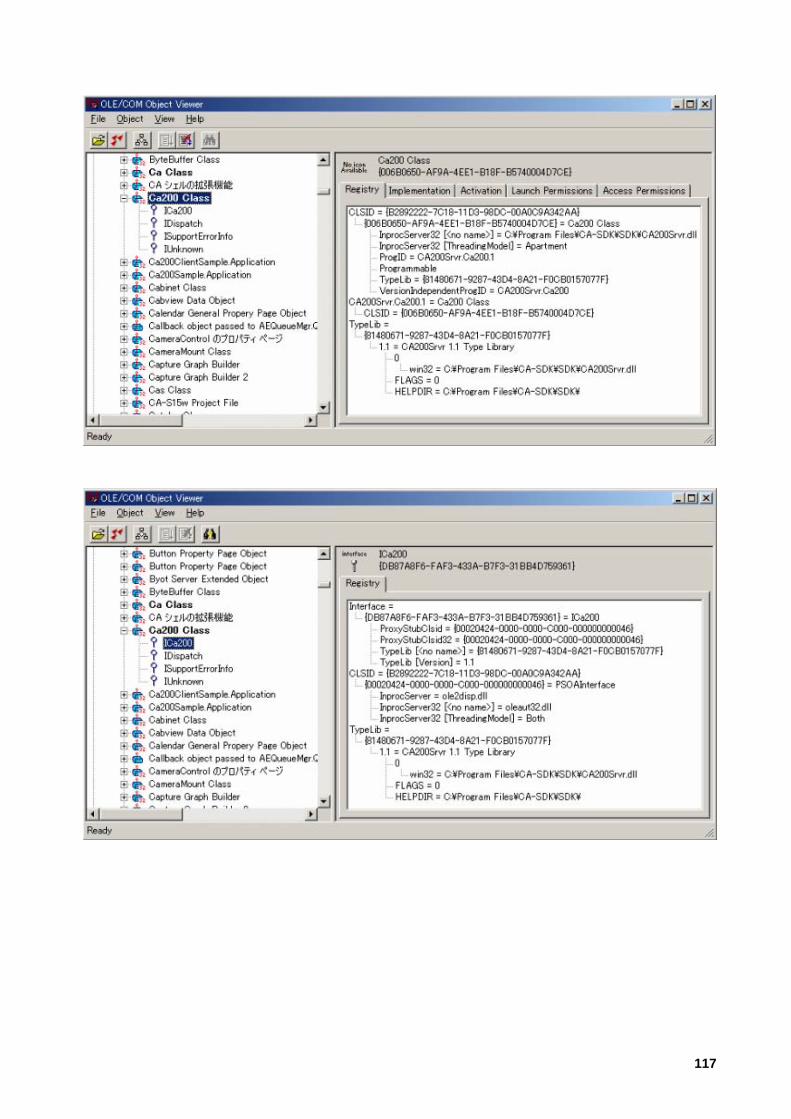
117

4-1-2: Automation
When using a COM object in a script language program, since that program itself doesn't have binary code, it is not possible to access individual interface binary structures. The function called automation is provided to handle this. In pure automation (not automation via a dual interface), the dispinterface statement is defined in the interface definition, but the implementation is actually done by the previously described IDispatch.
VC++'s MFC supports this (pure) automation. In automation, in order to create an object and enable the interface methods and properties to be referred to by the script, the "names" are used. These names are then handled by the special IDispatch interface, and the component calls are performed called indirectly. The CA-SDK events are programmed as if this dispinterface is defined. An application creation example using MFC for event control is explained in section 4-2: Creating a VC++ application using the CA-SDK.
If tool support is not used, it is necessary to program the IDispatch interface by hand. There are a variety of implementation methods, but it is complicated compared to a custom interface. When creating an entirely new component from scratch, if normal automation functions are sufficient, it is best to use tool support as much as possible.
118

4-1-3: Regarding COM
As an introduction to thinking about COM and COM components, let's consider another type of system.
Building my own AV system by selecting and combining various components, such as audio amplifiers, sound processors, CD/DVD players, video monitors, etc. has always been a dream of mine. But when I start to try and make this dream a reality, I run into problems. First, I don't have the latest components. Then, there is a problem with space, so it's unlikely I can make my dream come true in the near future. But if I can ignore such current problems, I can make my dream a reality even now. If I go to a specialty store, I can buy a variety of high-level components for connoisseurs. Once I get all the components I need, I connect them with cables. But even for cables, there are a wide range of grades available. What kind of pin plating, what kind of core, etc. Regardless of the grade, the function is the same: it's a "standard" cable. If I connect the components with this "standard" cable, then everything will be OK, and regardless of what CD or DVD I insert into the player, I get wonderful sound and/or video. Each component converts standard input to standard output, and transfers the results via the standard cable, and the various parts function well together. If I decide later that I don't like something, I can simply replace the component that I don't like with a different component.
Sorry for the long introduction. Now I'd like to explain COM in relation to that introduction.
Even in the field of software, if it was possible to create a program in the same way as creating the AV system described above, then the current situation of "dangerous" or "buggy" software would be greatly improved. Componentization of software. Using and reusing components. Software created in this way is referred to as "componentware".
The COM object model is the framework for creating componentware according to the specifications defined by Microsoft, and designates a set of services (implemented and offered by Windows). Components created using COM are referred to as COM components.
Whether we realize it or not, those of us using Windows computers are receiving a wide range of benefits from COM. OLE functions such as object embedding, transfer to the clipboard, and drag & drop, and macro functions which are supported by automation have become essential for doing work on the computer. Program developers use controls provided by Microsoft and other companies for creating GUIs or using databases to make programming of advanced functions easier. All of these are based on COM.
In this way, while COM itself is not center stage, it supports the Windows operating system from behind the scenes.
Conventionally, even for the Windows system, in order to expose a function to the outside, it is necessary to make it a function and offer it packaged in a DLL. In a DLL, a set of public functions are arranged flatly, and are called directly when creating a program.
COM uses the object-oriented programming paradigm. A COM component exposes a class, and the class exposes an interface. The interface lists the methods and functions available.
In object-oriented programming, programs are designed to simulate real-world events in software. Classes and objects express the things which exist and operate in that world, and how these things operate and interact is defined by the interface and methods.
People who have created a macro in Excel may have seen a class-level diagram. In Excel, data is organized into units called "books". In the data structure, a book is comprised of sheets and sheets are comprised of cells. We select a sheet or cell, perform some operation, and process the data. The object level in Excel is constructed to reflect this structure, and each sheet object or cell object has a collection of methods corresponding to the operations which we perform. In the world of Excel, these methods are visible to us and we use them to perform operations. If we can use this object level to simulate the necessary data processing in the software and design our software in this way, we can concentrate on obtaining solutions instead of worrying about the software situation.
119

COM does not use the conventional flat structure API, but instead offers a class-level API which simulates the real-world structure without depending on the development language or tool used.
Since the introduction of COM, it's been stated that Microsoft has used COM components to extend the Windows operating system. In Windows 2000, COM has been succeeded by COM+. In Windows 2000, there is even closer integration between the OS and COM, and many of the important functions provided by Windows 2000 are deeply linked to the advanced structure of COM+.
The keywords for understanding these advances are Windows DNA and DCE. In the beginning, a network was just a way for communicating between computers. The system environment in which programs ran operated on each computer in the network as if they were isolated islands. The popularization of the internet in this situation resulted in major changes. A 2-layered client/server model quickly became popular, and the network environment became a place for system activities.
COM is said to offer an exceptional operating environment in an intranet environment. The COM component can be used wherever it is on the network and programs can operate independent of that location. In addition, in Windows 2000, COM has been succeeded by COM+, which is said to offer sufficient infrastructure for the construction of mission-critical distributed systems for enterprises.
120

4-2: Creating a VC++ application using the CA-SDK
4-2: Creating a VC++ application using the CA-SDK
This section will explain how to create a CA-SDK application using the #import directive extension function of the VC++ compiler.
• For information on creating an application using the MFC COM support functions, there is a partial explanation in section 4-3: CA-SDK Sample Software Control Methods.
• For more detailed information on using the development tool for creating the sample software, please see section 4-2-2: Creating the SDK Application (Detailed Explanations).
• The sample software described herein assumes that the CA-SDK has been installed in the folder "C:\Program Files\CA-SDK". If the software has been installed in a different folder, please be sure to set the appropriate path description in the #import statements in the files "Ca200SampleDlg.h" and "Ca200SampleDlg.cpp".
121

4-2-1: Creating the SDK Application
4-2-1-1: Creating the Application Project
The sample software project will be as described below:
� The software will be a dialog-based application using MFC.
� The project name will be "Ca200Sample", and automation support will be enabled to allow CA-SDK event handling
122

4-2-1-2: Creating the UI (User Interface)
The UI (user interface) will be as shown below. There are a total of 10 static text controls (5 as labels and 5 for displaying measurement data) and 3 push buttons visible. The "OK" push button is the button created by default by VC++.
Set the following IDs for the static text controls for displaying data and the push buttons:
Lv display: IDC_STATIC_LV
x display: IDC_STATIC_X
y display: IDC_STATIC_Y
T diplay: IDC_STATIC_T
duv display: IDC_STATIC_DUV
Measure button:
IDC_BUTTON_MSR
Cal Zero button:
IDC_BUTTON_CAL0
Set the "Disabled" property of the "Measure" button to checked, and set the "Visible" property of the "Cancel" button (created by default by VC++) to unchecked.
123

4-2-1-3: Adding Code for the UI Objects
Add the BN_CLICKED message handlers for the Measure button and Cal Zero button.
Add the following DDX members to the static text controls for displaying measurement values.
Lv display: CString m_strLv;
x display: CString m_strx;
y display: CString m_stry;
T diplay: CString m_strT;
duv display: CString m_strduv;
124

4-2-1-4: CA-SDK Programming
4-2-1-4-1: CA-SDK Object Creation
This section will begin the explanation of creating the code for controlling the CA using the CA-SDK.
First, the objects provided by the CA-SDK need to be created and initialized to enable the CA-SDK to be used. This is done using the #import directive, a COM support function of VC++.
The type library is packaged as a resource in the file CA200Srvr.dll, one of the components of the CA-SDK. This file will be set as the type library specification for the #import directive.
� The #import directive statement should be added to the files "Ca200SampleDlg.h" and "Ca200SampleDlg.cpp" as shown in the code listings below.
Ca200SampleDlg.h
...
#if !defined(AFX_CA200SAMPLEDLG_H__ACD091F1_B9F2_4561_8FD0_F7D37051F8AC__INCLUDED_)
#define AFX_CA200SAMPLEDLG_H__ACD091F1_B9F2_4561_8FD0_F7D37051F8AC__INCLUDED_
//CA-SDK
#import "C:\Program Files\CA-SDK\SDK\CA200Srvr.dll" no_namespace no_implementation
...
Ca200SampleDlg.cpp
...
#include "Ca200SampleDlg.h"
#include "DlgProxy.h"
//CA-SDK
#import "C:\Program Files\CA-SDK\SDK\CA200Srvr.dll" no_namespace implementation_only
...
125

If build is performed at this point, the files "CA200Srvr.tlh" and "CA200Srvr.tli" are automatically created. "CA200Srvr.tli" contains the classes ICa200Ptr, ICasPtr, etc. (hereafter referred to as "smart pointers") created for the interfaces ICa200, ICas, etc. provided in "CA200Srvr.dll".
� Add the automatically generated smart pointer type Public member variables to the main window class Ca200SampleDlg.
Variable Type Variable Name
IOutputProbesPtr
m_pOutputProbesObj
IProbesPtr m_pProbesObj
ICasPtr m_pCasObj
IMemoryPtr m_pMemoryObj
IProbePtr m_pProbeObj
ICaPtr m_pCaObj
ICa200Ptr m_pCa200Obj
• Add the code for creating and initializing the CA-SDK objects (shown in the code listing below) to the main window initialization function "OnInitDialog().
In the code, initialization is performed using the SetConfiguration method to allow multiple CA units and multiple probes to be used.
• Create the Ca200 object ( )
• Using the SetConfiguration() method, set the program to use 1 CA unit with the following settings ( ):
• CA unit CA number = 1
• Probe: 1 connected, probe number = 1
• USB connection
From on, the settings for the objects for controlling the CA unit within the CA-SDK object level are performed.
• Obtain the Cas collection from the Ca200 object.
• Obtain the Ca object from the Cas object.
• Obtain the OutputProbes collection from the Ca object.
• Reset the OutputProbes collection.
• Add probe #1 to the OutputProbes collection and set it as the output probe.
• Obtain the Probe object from the OutputProbes collection
• Obtain the Memory object from the Ca object.
Then, from on, the various objects are used to perform the following CA unit initialization and memory channel settings:
• Set synchronization mode to NTSC.
126

• Set FAST/SLOW mode to FAST.
• Set analog display range to 2.5%, 2.5%.
• Set output display to Lvxy.
• Set the number of display digits to 4.
• Set memory channel to 0 (Konica Minolta calibration).
For more detailed information regarding these procedures, refer to Programming Guide, Section 3: "Creating a program using the SDK", 3.1 "Basic reference".
Ca200SampleDlg.cpp
...
BOOL CCa200SampleDlg::OnInitDialog()
{
...
// TODO: Add extra initialization here
//CA-SDK
long lcan = 1;
_bstr_t strcnfig(_T("1"));
long lprt = PORT_USB;
long lbr = 38400;
_bstr_t strprbid(_T("P1"));
_variant_t vprbid(_T("P1"));
try{
m_pCa200Obj = ICa200Ptr(__uuidof(Ca200));
m_pCa200Obj->SetConfiguration(lcan, strcnfig, lprt, lbr);
}
catch(_com_error e){
CString strerr;
strerr.Format(_T("HR:0x%08x\nMSG:%s"), e.Error(), (LPCSTR)e.Description());
AfxMessageBox((LPCSTR)strerr);
return TRUE;
}
127

m_pCasObj = m_pCa200Obj->Cas;
m_pCaObj = m_pCasObj ->ItemOfNumber[lcan];
m_pOutputProbesObj = m_pCaObj ->OutputProbes;
m_pOutputProbesObj ->RemoveAll();
m_pOutputProbesObj ->Add(strprbid);
m_pProbeObj = m_pOutputProbesObj ->Item[vprbid];
m_pMemoryObj = m_pCaObj->Memory;
m_pCaObj->SyncMode = SYNC_NTSC;
m_pCaObj->AveragingMode = AVRG_FAST;
m_pCaObj->SetAnalogRange(2.5, 2.5);
m_pCaObj->DisplayMode = DSP_LXY;
m_pCaObj->DisplayDigits = DIGT_4;
m_pMemoryObj->ChannelNO = 0;
...
}
...
128
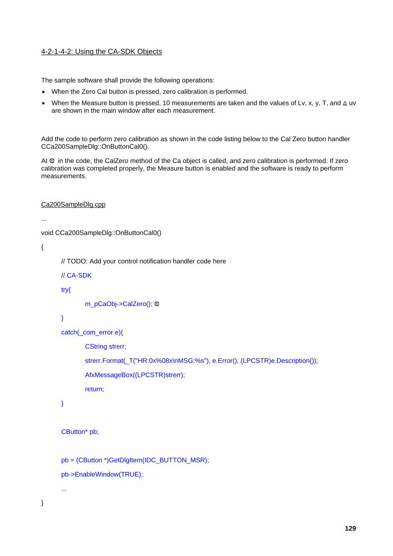
4-2-1-4-2: Using the CA-SDK Objects
The sample software shall provide the following operations:
• When the Zero Cal button is pressed, zero calibration is performed.
• When the Measure button is pressed, 10 measurements are taken and the values of Lv, x, y, T, and uv are shown in the main window after each measurement.
Add the code to perform zero calibration as shown in the code listing below to the Cal Zero button handler CCa200SampleDlg::OnButtonCal0().
At in the code, the CalZero method of the Ca object is called, and zero calibration is performed. If zero calibration was completed properly, the Measure button is enabled and the software is ready to perform measurements.
Ca200SampleDlg.cpp
...
void CCa200SampleDlg::OnButtonCal0()
{
// TODO: Add your control notification handler code here
// CA-SDK
try{
m_pCaObj->CalZero();
}
catch(_com_error e){
CString strerr;
strerr.Format(_T("HR:0x%08x\nMSG:%s"), e.Error(), (LPCSTR)e.Description());
AfxMessageBox((LPCSTR)strerr);
return;
}
CButton* pb;
pb = (CButton *)GetDlgItem(IDC_BUTTON_MSR);
pb->EnableWindow(TRUE);
...
}
129

...
Add the code to perform measurements as shown in the code listing below to the Measure button handler CCa200SampleDlg::OnButtonMsr().
At in the code, the Measure method of the Ca object is called, and measurement is performed. From on, the measurement results are obtained from the Probe object properties and set in the associated DDX members of the measurement results displays, and finally reflected in the controls.
Ca200SampleDlg.cpp
...
void CCa200SampleDlg::OnButtonMsr()
{
// TODO: Add your control notification handler code here
// CA-SDK
int i;
float fLv;
float fx;
float fy;
long lT;
float fduv;
for (i = 0; i < 10; i++){
m_pCaObj->Measure(0);
fLv = m_pProbeObj ->Lv;
fx = m_pProbeObj ->sx;
fy = m_pProbeObj ->sy;
lT = m_pProbeObj ->T;
fduv = m_pProbeObj ->duv;
m_strLv.Format("%4.2f",fLv);
m_strx.Format("%1.4f",fx);
m_stry.Format("%1.4f",fy);
m_strT.Format("%4d",lT);
m_strduv.Format("%1.4f",fduv);
130

UpdateData(FALSE);
}
}
...
131

4-2-1-4-3: Creating the Sink Object
The CA-SDK is equipped with a function for using an event to notify when the CA unit requires zero calibration. In order to use this function, the application must be equipped with an object to receive the event (hereafter referred to as a "sink object").
First, the sink object class will be created in the sample software:
Add the sink object class to the project.
• Class name: CCaEvent
• Base class: CcmdTarget
• Automation support: On
Replace the uuid value of the dispinterface added to the sample software .odl file with the uuid value defined in the _IcaEvents declarations section of the "CA200Srvr.tlh" file created by the import directive, as shown in the code list below.
Add an automation method to the CCaEvent.
• External name: ExeCalZero()
• Return value: void
This will become the sink interface/sink object class which can be received by the CA-SDK.
Ca200Sample.odl ...
// Primary dispatch interface for CCaEvent
//CA-SDK
// [ uuid(F73E02B5-6AEE-4099-969B-C1F81D043932) ]
[uuid(f7663750-5900-45eb-905f-78c5d5378481) ]
dispinterface ICaEvent
...
The IID_ICaEvent definition in the CaEvent implementation file should also be modified in the same way. (Since the format is somewhat different, be careful when making this modification.) Also, remove the static inherited member.
Add the extern declaration for IID_IcaEvent to the CaEvent definition file.
This will enable the code created in the following sections to reference this IID.
132

CaEvent.cpp
...
//CA-SDK
// {8DCF1114-787E-446C-BF4F-D283C178FA49}
//static const IID IID_ICaEvent =
//{ 0x8dcf1114, 0x787e, 0x446c, { 0xbf, 0x4f, 0xd2, 0x83, 0xc1, 0x78, 0xfa, 0x49 } };
//f7663750-5900-45eb-905f-78c5d5378481
const IID IID_ICaEvent =
{ 0xf7663750, 0x5900, 0x45eb, { 0x90, 0x5f, 0x78, 0xc5, 0xd5, 0x37, 0x84, 0x81 } };
...
CaEvent.h
...
//CA-SDK
extern const IID IID_ICaEvent;
/////////////////////////////////////////////////////////////////////////////
// CCaEvent command target
class CCaEvent : public CCmdTarget
{
DECLARE_DYNCREATE(CCaEvent)
...
Add the event-handling code for CCaEvent::ExeCalZero() as shown below.
In the sample software, when the event occurs, the Measure button is disabled.
CaEvent.cpp
...
133
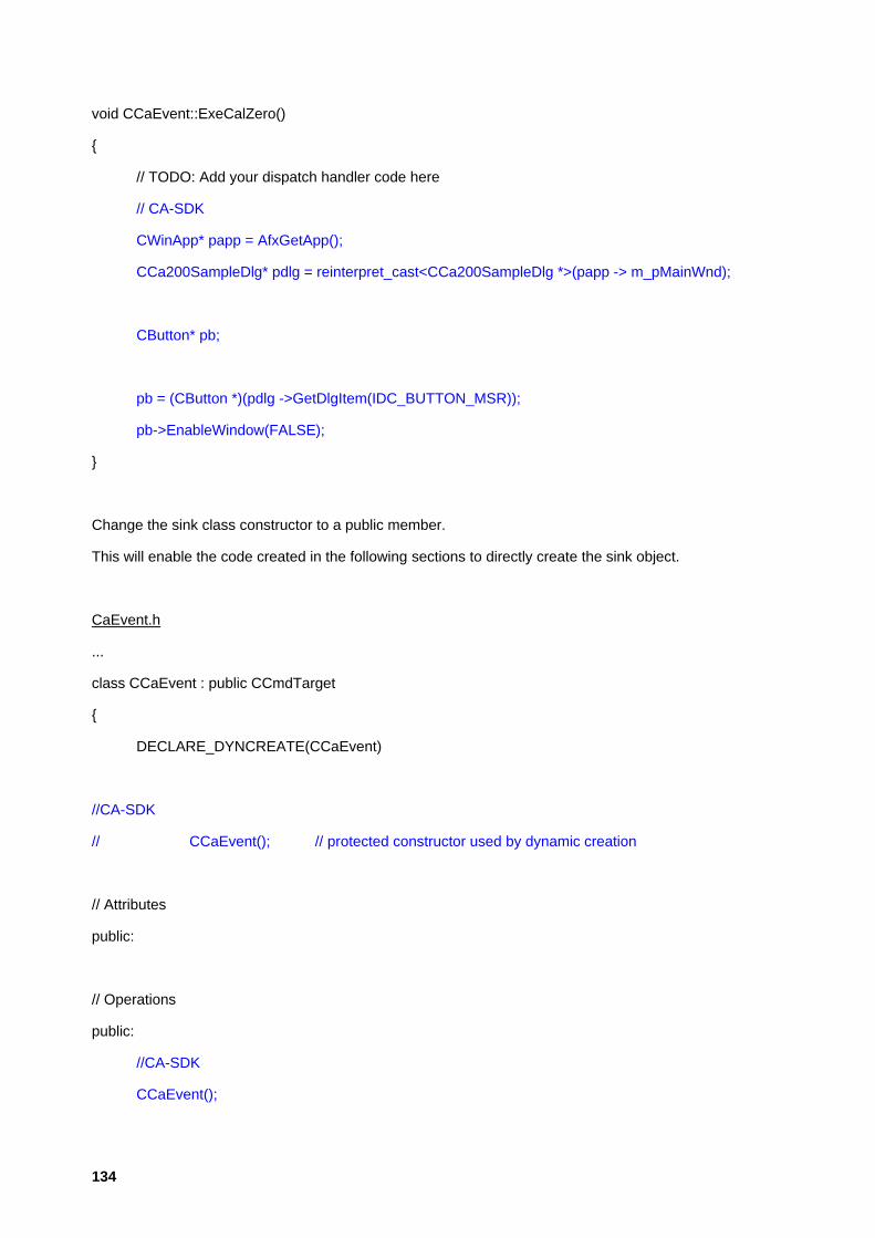
void CCaEvent::ExeCalZero()
{
// TODO: Add your dispatch handler code here
// CA-SDK
CWinApp* papp = AfxGetApp();
CCa200SampleDlg* pdlg = reinterpret_cast<CCa200SampleDlg *>(papp -> m_pMainWnd);
CButton* pb;
pb = (CButton *)(pdlg ->GetDlgItem(IDC_BUTTON_MSR));
pb->EnableWindow(FALSE);
}
Change the sink class constructor to a public member.
This will enable the code created in the following sections to directly create the sink object.
CaEvent.h
...
class CCaEvent : public CCmdTarget
{
DECLARE_DYNCREATE(CCaEvent)
//CA-SDK
// CCaEvent(); // protected constructor used by dynamic creation
// Attributes
public:
// Operations
public:
//CA-SDK
CCaEvent();
134

...
};
...
Add the file "Ca200SampleDlg.h" to the included files in CaEvent.cpp: // CaEvent.cpp : implementation file
//
#include "stdafx.h"
#include "Ca200Sample.h"
#include "CaEvent.h"
#include "Ca200SampleDlg.h"
...
Finally, add the following Public member variables to the main window class Ca200SampleDlg.
Variable Type Variable Name
IConnectionPointPtr
m_pIConnectionPointObj
IDispatch* m_pIDispatch
DWORD m_dwCk
135

4-2-1-4-4: Sink Object Creation/Connection and Event Handling
Add the sink object creation and connection code shown below to the CCa200SampleDlg::OnInitDialog() after the initialization code previously created.
IConnectionPointPtr and IConnectionPointContainerPtr are smart pointers for the objects which perform CA-SDK event handling. These are the so-called standard interface defined by MS. The smart pointers of the standard interface have already been defined, and the header file is included in CA200Srvr.tlh.
In the code:
creates the sink object.
obtains the sink interface to that object.
finds the object (IConnectionPoint interface connection point) for connecting to the sink interface.
adds a connection to that object.
stores the ID required for terminating the connection later.
Ca200SampleDlg.cpp
BOOL CCa200SampleDlg::OnInitDialog()
...
m_dwCk = 0;
CCaEvent* pevntobj;
if (NULL != (pevntobj = new CCaEvent)){ {bmc circle1.bmp}
m_pIDispatch = pevntobj ->GetIDispatch(FALSE);
IConnectionPointContainerPtr pcpcobj;
DWORD dwck;
pcpcobj = m_pCaObj;
pcpcobj -> FindConnectionPoint(IID_ICaEvent, &m_pIConnectionPointObj);
m_pIConnectionPointObj ->Advise(m_pIDispatch, &dwck);
m_dwCk = dwck;
}
136
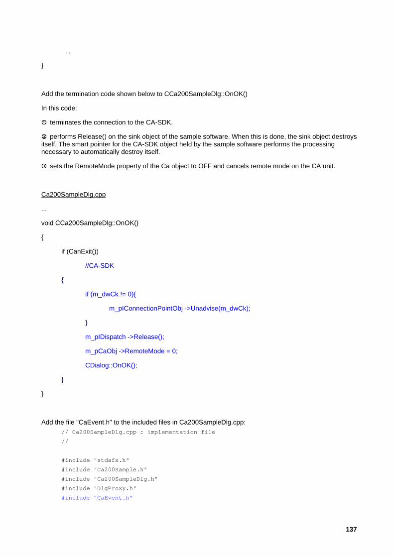
...
}
Add the termination code shown below to CCa200SampleDlg::OnOK()
In this code:
terminates the connection to the CA-SDK.
performs Release() on the sink object of the sample software. When this is done, the sink object destroys itself. The smart pointer for the CA-SDK object held by the sample software performs the processing necessary to automatically destroy itself.
sets the RemoteMode property of the Ca object to OFF and cancels remote mode on the CA unit.
Ca200SampleDlg.cpp
...
void CCa200SampleDlg::OnOK()
{
if (CanExit())
//CA-SDK
{
if (m_dwCk != 0){
m_pIConnectionPointObj ->Unadvise(m_dwCk);
}
m_pIDispatch ->Release();
m_pCaObj ->RemoteMode = 0;
CDialog::OnOK();
}
}
Add the file "CaEvent.h" to the included files in Ca200SampleDlg.cpp: // Ca200SampleDlg.cpp : implementation file
//
#include "stdafx.h"
#include "Ca200Sample.h"
#include "Ca200SampleDlg.h"
#include "DlgProxy.h"
#include "CaEvent.h"
137

138

4-2-1-4-5: Error Handling
The smart pointers generated by the #import directive also wrap the COM error handling procedures. If a call from the CA-SDK fails, a _com_error type irregular object is thrown.
In the sample software, the HRESULT value at the time the error occurred from the irregular object or the CA-SDK error message is obtained and shown in a message box.
Ca200SampleDlg.cpp
BOOL CCa200SampleDlg::OnInitDialog()
{
...
try{
m_pCa200Obj = ICa200Ptr(__uuidof(Ca200));
m_pCa200Obj->SetConfiguration(lcan, strcnfig, lprt, lbr);
}
catch(_com_error e){
CString strerr;
strerr.Format(_T("HR:0x%08x\nMSG:%s"), e.Error(), (LPCSTR)e.Description());
AfxMessageBox((LPCSTR)strerr);
return TRUE;
}
...
}
139
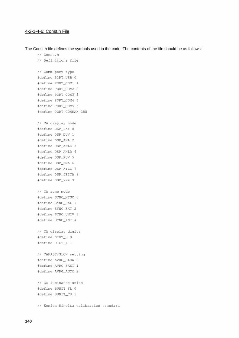
4-2-1-4-6: Const.h File
The Const.h file defines the symbols used in the code. The contents of the file should be as follows: // Const.h
// Definitions file
// Comm port type
#define PORT_USB 0
#define PORT_COM1 1
#define PORT_COM2 2
#define PORT_COM3 3
#define PORT_COM4 4
#define PORT_COM5 5
#define PORT_COMMAX 255
// CA display mode
#define DSP_LXY 0
#define DSP_DUV 1
#define DSP_ANL 2
#define DSP_ANLG 3
#define DSP_ANLR 4
#define DSP_PUV 5
#define DSP_FMA 6
#define DSP_XYZC 7
#define DSP_JEITA 8
#define DSP_XYZ 9
// CA sync mode
#define SYNC_NTSC 0
#define SYNC_PAL 1
#define SYNC_EXT 2
#define SYNC_UNIV 3
#define SYNC_INT 4
// CA display digits
#define DIGT_3 0
#define DIGT_4 1
// CAFAST/SLOW setting
#define AVRG_SLOW 0
#define AVRG_FAST 1
#define AVRG_AUTO 2
// CA luminance units
#define BUNIT_FL 0
#define BUNIT_CD 1
// Konica Minolta calibration standard
140

#define CAL_D65 1
#define CAL_9300 2
#define CAL_CA100 3
// CA type
#define CATYPE_210 0
#define CATYPE_210S 1
#define CATYPE_100PLUS 2
#define CATYPE_200 3
// Probe type
#define PROBETYPE_CA100PLUS 1001
#define PROBETYPE_CA100PLUSH 1002
#define PROBETYPE_CA210 2100
#define PROBETYPE_CA210S 2101
// Remote mode
#define REMOTE_OFF 0
#define REMOTE_ON 1
#define REMOTE_LOCK 2
// Reference color
#define CAL_RED 0
#define CAL_GREEN 1
#define CAL_BLUE 2
#define CAL_WHITE 3
After the "Const.h" file has been created, add the file to the included files in Ca200SampleDlg.cpp: // Ca200SampleDlg.cpp : implementation file
//
#include "stdafx.h"
#include "Ca200Sample.h"
#include "Ca200SampleDlg.h"
#include "DlgProxy.h"
#include "CaEvent.h"
#include "Const.h"
141
4-2-2: Creating the SDK Application (Detailed Explanations)
4-2-2: Creating the SDK Application (Detailed Explanations)
Currently, many development environments provide support for COM components. However, how to use that support varies, and accordingly, how an application is developed also varies.
When programming in MS Visual Basic (hereafter referred to as VB), no special attention is necessary to use COM components. Using the VB COM support functions, programming can be performed in the same way as using other VB-specific objects. However, when using C/C++, there are several methods of including the COM objects (similar to how other applications are included), and the developer must choose the method to use.
In MS Visual C++ (hereafter referred to as VC++), one of the choices is to use the #import directive extension function of the VC++ compiler. This method enables development of a program almost as easily as using VB. In addition, since this is a compiler function, it can be used even for applications which do not use the framework offered by tools such as MFC/ATL, etc. Previous VC++ applications "handmade" using VC++ can be reused and programming to include the CA-SDK is simplified.
142
4-2-2-1: Creating the Application Project
The sample software will be a dialog-based application using MFC. The process for creating the MFC application will be explained according to the following outline:
Step 1: Creating the project.
Step 2: Creating the UI (user interface).
Step 3: Adding the code for handling the UI objects.
Step 4: Adding the code for the application itself.
Step 5: Compiling and debugging.
In this section, we will explain Step 1: Creating the project using the application wizard tool of VC++. As you answer the questions in the application wizard, the necessary objects and code skeleton will be created automatically.
For the sample software, the settings described below should be used.
Start VC++, and select New... from the File menu; the Application Wizard will start. In the New dialog, perform the following settings:
1 Select the "Projects" tab.
2 Select "MFC AppWizard (exe)" from the list of project types.
3 Specify the desired project folder in the "Location" box.
4 Input the desired project name in the "Project name" box.
5 Other settings can be left at their default settings ("Create new workspace" selected; "Win32" checked in "Platforms").
Then click OK.
143

In the "MFC AppWizard - Step 1" dialog which appears,
� Set "What type of application would you like to create?" to "Dialog based".
� Leave "What language would you like your resources in?" set to the default setting.
144

and click Next.
In the "MFC AppWizard - Step 2 of 4" dialog which appears,
� Check "Automation" in "What other support would you like to include?"
� Leave other settings at their default settings ("About box" and "3D controls" checked for "What features would you like to include?", "ActiveX Controls" checked in "What other support would you like to include?", "Windows Sockets" not checked in "Would you like to include WOSA support?", and the dialog title left at the automatically created title).
and click Next.
In the "MFC AppWizard - Step 3 of 4" dialog which appears,
145

� Leave all settings at their defaults ("MFC Standard" for "What style of project would you like?", "Yes, please" for "Would you like to generate source file comments?", and "As a shared DLL" for "How would you like to use the MFC library?")
and click Next.
Check the information in the "MFC AppWizard - Step 4 of 4" dialog which appears and click Finish.
146
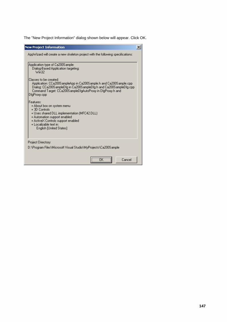
The "New Project Information" dialog shown below will appear. Click OK.
147

4-2-2-2: Creating the UI (User Interface)
For Step 2: Creating the UI (user interface), the Resource Editor should be used.
Select the "ResourceView" tab in the workspace, expand the "Dialog" folder by clicking on the "+" next to it, and then double-click on the dialog which will be the main window in the project ("IDD_CA200SAMPLE_DIALOG"). A default dialog will appear, with the buttons "OK" and "Cancel" already provided.
Edit the dialog so that it is as shown in section 4-2-1-2: Creating the UI (User Interface), adding 10 static text controls (5 for labels, 5 for displaying measurement values) and 2 new push buttons.
Editing of the dialog can be performed in the same way as in VB. Select the necessary control from the Tool Control Box in the editor window, drag it onto the dialog, and drop it in position. Changing the position or size of controls already placed on the dialog is also the same as in VB.
After the main settings have been completed, right-click on a control and select Properties from the menu which appears to open the Properties dialog for editing the control properties.
For example, for the static text for the "Lv:" label, right-click on the control and select Properties from the menu which appears to open the Properties dialog, and set "Lv:" as the "Caption:" for the control.
Repeat for the remaining static text labels, setting the Captions as shown in the dialog in section 4-2-1-2: Creating the UI (User Interface).
For the static text controls which will be used to display the measurement values, set the Caption to nothing and set the IDs as listed in section 4-2-1-2: Creating the UI (User Interface) so that they can be remembered easily when accessing them later from the source code.
Also, check the "Sunken" property in the "Style" tab of the Properties dialog so that there will be a sunken frame around the values.
148

Also change the Caption and ID for the push buttons to those shown in section 4-2-1-2: Creating the UI (User Interface),
and uncheck the Visible property in the "General" tab for the default "Cancel" button (so that the button will not be shown).
Finally, use the items in the Layout menu to adjust the size and spacing of the controls to make the dialog look good overall.
149
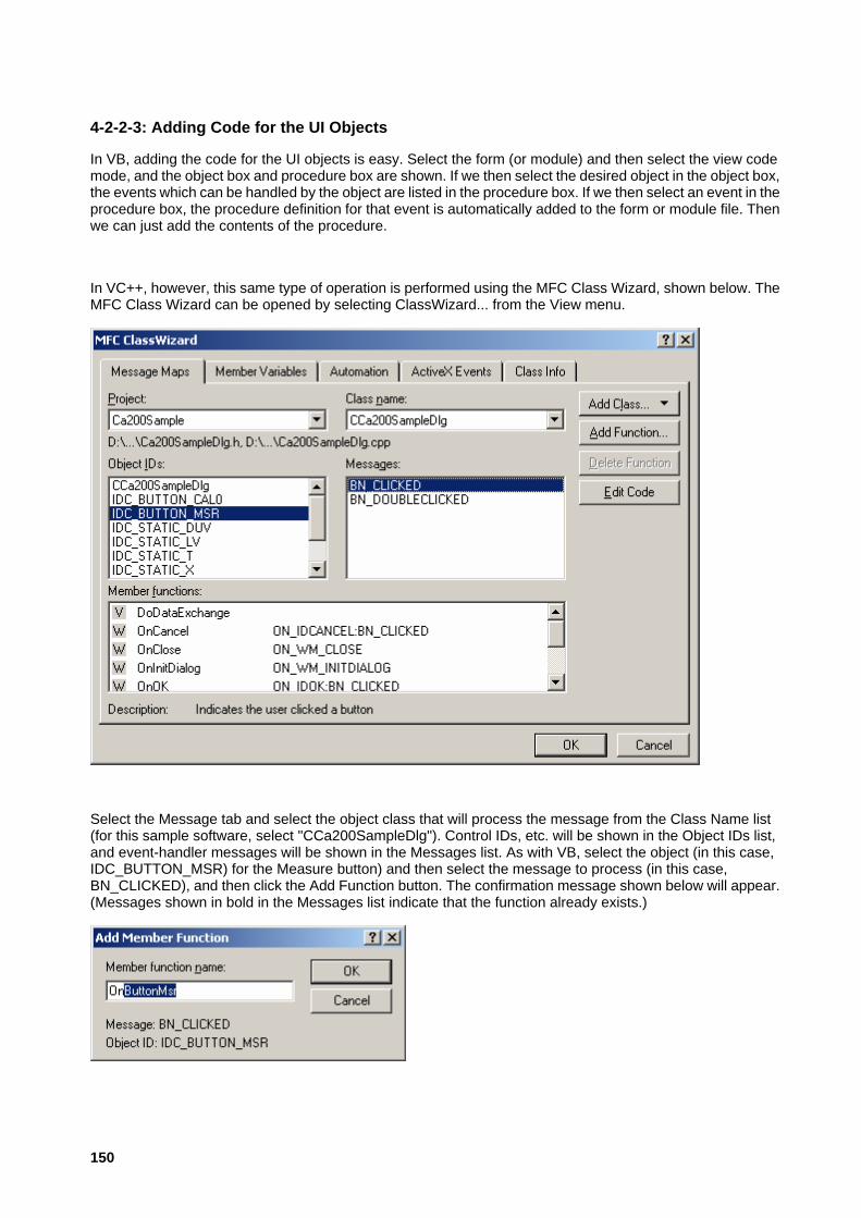
4-2-2-3: Adding Code for the UI Objects
In VB, adding the code for the UI objects is easy. Select the form (or module) and then select the view code mode, and the object box and procedure box are shown. If we then select the desired object in the object box, the events which can be handled by the object are listed in the procedure box. If we then select an event in the procedure box, the procedure definition for that event is automatically added to the form or module file. Then we can just add the contents of the procedure.
In VC++, however, this same type of operation is performed using the MFC Class Wizard, shown below. The MFC Class Wizard can be opened by selecting ClassWizard... from the View menu.
Select the Message tab and select the object class that will process the message from the Class Name list (for this sample software, select "CCa200SampleDlg"). Control IDs, etc. will be shown in the Object IDs list, and event-handler messages will be shown in the Messages list. As with VB, select the object (in this case, IDC_BUTTON_MSR) for the Measure button) and then select the message to process (in this case, BN_CLICKED), and then click the Add Function button. The confirmation message shown below will appear. (Messages shown in bold in the Messages list indicate that the function already exists.)
150

When OK is clicked, the necessary code will be inserted into the associated files. After that, as with VB, you can add the contents of the function.
Add the BN_CLICKED message handler for the Cal Zero button in the same way.
The MFC Class Wizard is used in a variety of cases other than for creating message handlers as described above. In the sample software, the MFC DDX (Dialog Data Exchange) function is used. This function associates dialog member variables with the controls in a dialog. The settings for this function are also handled by the MFC Class Wizard.
In the sample software, we will associate member variables of the dialog (which functions as the main window) with the static text controls for displaying the measurement data. Open the MFC Class Wizard and select the Member Variables tab. Select the class for which settings will be made ("CCa200SampleDlg") from the Class name list. Then, in the Control IDs list, select the control ID "IDC_STATIC_LV" (for the control which will display the Lv data) and click Add Variable.
The Add Member Variable dialog shown below will appear. Input "m_strLv" as the member variable name in the "Member variable name" box, set "Category:" to "Value", and set "Variable type:" to "CString", and then click OK.
151

This automatically creates the functions for transferring values back and forth between the static text control with the ID "IDC_STATIC_LV" and the m_strLv member of the CCa200SampleDlg C++ class of the sample software dialog.
Repeat this procedure for the remaining controls for displaying measurement data.
152
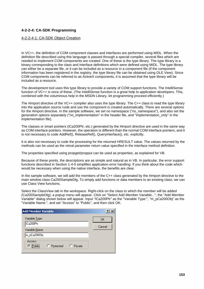
4-2-2-4: CA-SDK Programming
4-2-2-4-1: CA-SDK Object Creation
In VC++, the definition of COM component classes and interfaces are performed using MIDL. When the definition file described using this language is passed through a special compiler, several files which are needed to implement COM components are created. One of these is the type library. The type library is a binary corresponding to the class and interface definitions which were defined using MIDL. The type library can either be a separate file, or it can be included as a resource in a component file (if the component information has been registered in the registry, the type library file can be obtained using OLE View). Since COM components can be referred to as ActiveX components, it is assumed that the type library will be included as a resource.
The development tool uses this type library to provide a variety of COM support functions. The IntelliSense function of VC++ is once of these. (The IntelliSense function is a great help to application developers. This, combined with the voluminous help in the MSDN Library, let programming proceed efficiently.)
The #import directive of the VC++ compiler also uses the type library. The C++ class to read the type library into the application source code and use the component is created automatically. There are several options for the #import directive. In the sample software, we set no namespace ("no_namespace"), and also set the generation options separately ("no_implementation" in the header file, and "implementation_only" in the implementation file).
The classes or smart pointers (ICa200Ptr, etc.) generated by the #import directive are used in the same way as COM interface pointers. However, the operation is different than the normal COM interface pointers, and it is not necessary to code AddRef(), ReleaseRef(), QueryInterface(), etc. explicitly.
It is also not necessary to code the processing for the returned HRESULT value. The values returned by the methods can be used as the retval parameter return value specified in the interface method definition.
The properties specified using propget/propput can be used as properties, as explained for VB.
Because of these points, the descriptions are as simple and natural as in VB. In particular, the error support functions described in Section 1-4-5 simplifies application error handling. If you think about the code which would be necessary when using the native interface, the benefits are clear.
In the sample software, we will add the members of the C++ class generated by the #import directive to the main window class Ca200SampleDlg. To simply add functions or data members to an existing class, we can use Class View functions.
Select the ClassView tab in the workspace. Right-click on the class to which the member will be added (Ca200SampleDlg); a popup menu will appear. Click on "Select Add Member Variable..."; the "Add Member Variable" dialog shown below will appear. Input "ICa200Ptr" as the "Variable Type:", "m_pCa200Obj" as the "Variable Name:", and set "Access" to "Public", and then click OK.
153
This adds the specified member m_pCa200Obj to the main window class Ca200SampleDlg. Add the other member variables in the same way.
154

4-2-2-4-2: Using the CA-SDK Objects
Once the creation and initialization of the CA-SDK objects have been completed, the objects can be used to perform calibration, measurements, etc.
How to use the CA-SDK objects is explained in the CA-SDK Programming Guide. Although the explanation in the Programming Guide uses VB, if the code for this sample software is used as a reference, it should be simple to convert it to C++ code. See section 4-3: CA-SDK Sample Software Control Methods.
155
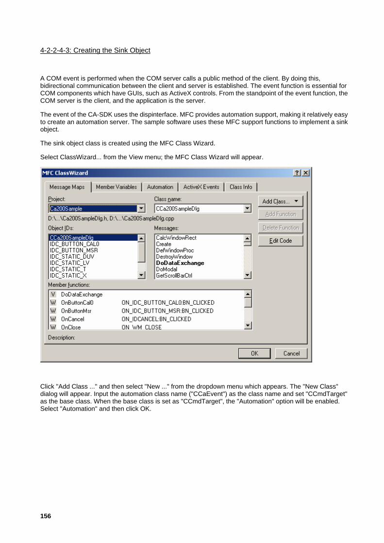
4-2-2-4-3: Creating the Sink Object
A COM event is performed when the COM server calls a public method of the client. By doing this, bidirectional communication between the client and server is established. The event function is essential for COM components which have GUIs, such as ActiveX controls. From the standpoint of the event function, the COM server is the client, and the application is the server.
The event of the CA-SDK uses the dispinterface. MFC provides automation support, making it relatively easy to create an automation server. The sample software uses these MFC support functions to implement a sink object.
The sink object class is created using the MFC Class Wizard.
Select ClassWizard... from the View menu; the MFC Class Wizard will appear.
Click "Add Class ..." and then select "New ..." from the dropdown menu which appears. The "New Class" dialog will appear. Input the automation class name ("CCaEvent") as the class name and set "CCmdTarget" as the base class. When the base class is set as "CCmdTarget", the "Automation" option will be enabled. Select "Automation" and then click OK.
156

The tool will then create the automation implementation class CCaEvent. In the application interface definition file (CA200Sample.odl), the definitions for the coclass (meaning "COM class") CCaEvent and its default dispinterface ICaEvent will be added. Automatically created class IDs and interface IDs for both will also be assigned.
Next, the MFC Class Wizard will be used to add the event method. Select the "Automation" tab, select the just-created "CCaEvent" as the "Class name:", and click "Add Method ..."; the Add Method dialog will appear. Input "ExeCalZero" for both the "External name:" and "Internal name:", select "void" as the "Return type:" and no parameters (as in the event definition), and then click OK.
157
Then click OK to close the MFC Class Wizard. This basically completes the definition of the sink object.
The tool will create the necessary .odl file and C++ file and code.
In order to use the created sink object for the CA-SDK event sink, it is necessary to manually modify one part of the automatically created code, and set the IID assigned automatically by the tool to the IID value specified by the CA-SDK. The COM interface can only recognize this identity using the GUID/uuid.
Search for the IIDs automatically assigned by the tool and replace them with the event IIDs recognized by the CA-SDK. By doing this, the created object will become an event sink recognized by the CA-SDK.
In addition, the changes described in section 4-2-1-4-3: Creating the Sink Object other than the implementation of ExeCalZero() are changes necessary to locally create and use this sink object. Normally, when operating as a server, the public objects are created by the so-called "class factory". The implementation of the COM class in MFC also handles this. In the sample software, in order to operate as a local object, some modifications were made to the automatically created definition and implementation files.
158
4-2-2-4-4: Sink Object Creation/Connection and Event Handling
CA-SDK events are handled using the standard interface IConnectionPoint connection point defined by MS for event handling. When a connection to the sink interface is established in the connection point object, the corresponding events are issued from the server and the sink interface method is called.
Establishing and terminating a connection to the sink interface is usually performed according to the following procedure:
1 An object supporting events calls the connection point container object and obtains the IConnectionPointContainer.
2 The FindConnectionPoint() method of IConnectionPointContainer is used to obtain the connection point object IConnectionPoint which supports the sink interface.
3 The Advise() method of IConnectionPoint is used to establish a connection to the sink object.
4 When event handling is no longer necessary, the UnAdvise() method of IConnection point is used to terminate the connection to the sink object.
159

4-2-2-4-5: Const.h File
In the sample software, the symbols used in the code are defined in the file "Const.h", which must be added to the project.
To create a new file and add it to the project, select "New" from the File menu. The New dialog will be shown.
Select the "File" tab, select the file type to be created ("C/C++ Header File"), check "Add to project", and select the "Ca200Sample" project. Type in the file name "Const" and click OK to create the file.
To add an existing file to the project, select the "FileView" tab of the workspace view, right-click on "Ca200Sample files", and select "Add Files to Project..." from the dropdown menu which appears. The Insert Files Into Project dialog will be shown. Browse to and select the file to add to the project and click OK to add the file to the project.
160

161

4-3: CA-SDK Sample Software Control Methods
4-3: CA-SDK Sample Software Control Methods
Three sample ActiveX controls are included in the CA-SDK VB sample software. Although they were originally written for use with the sample software, any of them can also be used by other software.
In this document, how to use the CaControl (a control for performing various settings on CA-series instruments) and the xyControl (a control for displaying measurement results on a graph of the xy color space) will be explained.
162
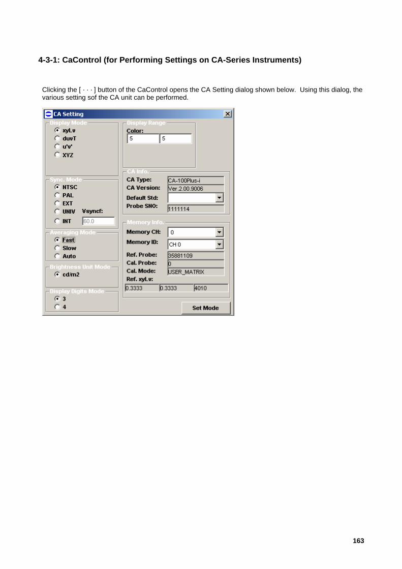
4-3-1: CaControl (for Performing Settings on CA-Series Instruments)
Clicking the [ · · · ] button of the CaControl opens the CA Setting dialog shown below. Using this dialog, the various setting sof the CA unit can be performed.
163

4-3-1-1: CaControl Properties/Methods
Ca property
Sets/retrieves property
Sets and retrieves the Ca object to which settings will be applied. Before doing anything else with the control, use this property to set the Ca object which will be controlled.
Syntax: Dim objCaControl as CaControl
Dim ObjCa as Ca
Set ObjCaControl.Ca = objCa
Probe property
Sets/retrieves property
Sets and retrieves the Probe object to which settings will be applied. Before doing anything else with the control, use this property to set the Probe object which will be controlled.
Syntax: Dim objCaControl as CaControl
Dim objProbe as Probe
Set ObjCaControl.Probe = objProbe
Memory property
Sets/retrieves property
Sets and retrieves the memory object to which settings will be applied. Before doing anything else with the control, use this property to set the Memory object which will be controlled.
Syntax: Dim objCaControl as CaControl
Dim objMemory as Memory
Set ObjCaControl.Memory = objMemory
UpdateCaInfo method
164

Updates the information (except the memory channel) displayed in the Ca control to reflect the current status of the CA unit.
After setting the required CA-SDK object, this method should be used once before doing anything else with the control.
Syntax: Dim objCaControl as CaControl
ObjCaControl.UpdateCaInfo
UpdateMemoryInfo method
Updates the memory channel displayed in the Ca control to reflect the currently set memory channel on the CA unit.
After setting the required CA-SDK object, this method should be used once before doing anything else with the control.
Syntax: Dim objCaControl as CaControl
ObjCaControl.UpdateMemoryInfo
Update event
This event is fired when the control has changed a setting for the CA unit.
165

4-3-1-2: CaControl: Using in VB
First, the CA-SDK component should be added to the VB project using the CA-SDK component reference settings. (How to perform the reference settings is described in the CA-SDK Programming Manual.)
Next, add the control to the VB project as follows:
1 Select "Components" from the Project menu. The "Components" dialog will appear.
166

2 In the "Controls" tab of the "Components" dialog, check the "KONICA MINOLTA CaControl" and click OK.
When the control has been successfully added, the control icon will be added to the Form Editor toolbox, and the control can be used in the editor.
The source code shown below is extracted from the CA-SDK Color measurement sample software.
After creating the SDK object, the objects for controlling the CA unit are set on the control using the control's properties ( , , ). (The control has been placed on the FormMeasurement form.)
Then, the current status of the CA unit is obtained and reflected in the control using UpdateCaInfo and UpdateMemoryInfo to initialize the control.
After performing the above procedure, the control is ready to be used.
When using the Update event, the control functions should be declared using the WithEvents keyword in the declaration section of the form on which the control has been placed. Selecting the control object in the object box in code edit mode will make it possible to select the "Update" procedure in the procedure box. The CaControl calls this Update handler when the CA unit settings have been changed.
Ca200Sample.basPublic Sub Main()
...
'===================================
' Create SDK/Application Object
'===================================
Set objCa200 = New Ca200
167

'===================================
' Set Configuration
'===================================
objCa200.AutoConnect
'===================================
' Initialize SDK Object
'===================================
Set objCa = objCa200.SingleCa
Set objProbe = objCa.SingleProbe
Set objMemory = objCa.Memory
...
Set FormMeasurement.objCaControl.Ca = objCa
Set FormMeasurement.objCaControl.Probe = objProbe
Set FormMeasurement.objCaControl.Memory = objMemory
...
FormMeasurement.objCaControl.UpdateCaInfo
FormMeasurement.objCaControl.UpdateMemoryInfo
FormMeasurement.frm Public WithEvents objCaControl As CaControl
...
Private Sub CaControl1_Update()
...
End Sub
168

4-3-1-3: CaControl: Using in VC++ (MFC)
How to use the control in an MFC application will be explained using sample software.
In section 4-2: Creating a VC++ application using the CA-SDK, the COM support functions of the VC++ compiler were used, but in this example, the MFC support functions will be used to create the application.
The sample software is a dialog-based application with the GUI shown below. The dialog items to the left of the "OK" and "Cancel" buttons comprise the CaControl which will be used this time. If you click on the "..." button, the previously described "CA Setting" dialog will appear.
When creating the project, enable the support option for ActiveX controls.
First, the CA-SDK component is added to the project as follows:
1 Select "ClassWizard ..." from the View menu. The MFC ClassWizard will appear.
2 Click the "Add Class ..." button, and select "From a type library ..." from the dropdown menu which appears.
3 In the "Import from Type Library" dialog which appears, browse to the folder containing the file "CA200Srvr.dll", select "CA200Srvr.dll", and click OK
169

4 The "Confirm Classes" dialog shown below will appear. After confirming the displayed information, click OK. You will return to the "MFC Class Wizard" dialog. Click OK to close the dialog.
This completes the process for adding the CA-SDK component to the project. The C++ wrapper classes (ICa200, ICas, etc.) for using the CA-SDK objects will be automatically created.
• If the project is built at this point, an error indicating that the SetChannelID() method of the IMemory class defined in the file "ca200Srvr.h" created automatically by the tool is defined twice will appear. This is because for the ChannelID property of the CA-SDK Memory object, the name of the settings wrapper method created automatically by the tool (SetChannelID) is colliding with the name of the SetChannelID method originally provided for the Memory object. It is therefore necessary to change one of the names. In the sample software, the name of the original method has been changed to SetID.
170

Next, the control will be added to the MFC project in order to use the control in the MFC application.
1 Select "Components and Controls ..." from the popout menu which appears when "Add to Project" is selected in the Project menu.
2 In the "Components and Controls Gallery" dialog which appears, select the "MinoltaCaControl.CaControl" from the "Registered ActiveX Controls" folder, and click "Insert".
171

3 When "OK" is clicked in the confirmation message box, the "Confirm Classes" dialog will appear. Check only the C_CaControl and click OK. The "Components and Controls Gallery" dialog of step 2 will reappear; click "Close" to close the dialog.
After this process has been completed, the CaControl is ready to be used.
The CaControl icon will be added to the Resource Editor toolbox. In addition, the C++ class C-CaControl for controlling the control confirmed in step 3 will be automatically created.
Then, the following must be performed to complete coding preparations:
1 Add the control class DDX member variable m_CCaControl to the dialog class.
2 Add the CA-SDK object class member variables m_ICa200, m_ICa, m_IProbe, and m_IMemory to the dialog class.
Source code from the sample software for using the control is shown below.
The Ca200 object is created.
The Ca object is obtained (from the SingleCa property) using the GetSingleCa method.
An instance of the wrapper class ICa for the Ca object is attached. Thereafter, the ICa instance is manipulated in the same way as a Ca object.
In the same way, the settings for the Probe object and Memory object are also performed. The code up to this point performs initialization of the CA-SDK objects.
172

Then, the Ca object, Probe object, and Memory object are set ( , , and ).
Finally, the CaControl is initialized using the control methods UpdateCaInfo and UpdateMemoryInfo.
This makes the control ready to use.
Test1Dlg.cppBOOL CTest1Dlg::OnInitDialog()
{
...
// TODO: Add extra initialization here
m_ICa200.CreateDispatch("CA200Srvr.Ca200.1");
m_ICa200.m_bAutoRelease = TRUE;
m_ICa200.AutoConnect();
LPDISPATCH pICa = m_ICa200.GetSingleCa();
m_ICa.AttachDispatch(pICa);
LPDISPATCH pIProbe = m_ICa.GetSingleProbe();
m_IProbe.AttachDispatch(pIProbe);
LPDISPATCH pMemory = m_ICa.GetMemory();
m_IMemory.AttachDispatch(pMemory);
m_ICa.CalZero();
m_CCaControl.SetRefCa(&m_ICa.m_lpDispatch);
m_CCaControl.SetRefProbe(&m_IProbe.m_lpDispatch);
m_CCaControl.SetRefMemory(&m_IMemory.m_lpDispatch);
m_CCaControl.UpdateCaInfo();
m_CCaControl.UpdateMemoryInfo();
return TRUE; // return TRUE unless you set the focus to a control
}
Compared to using the #import directive as in section 4-2: Creating a VC++ application using the CA-SDK, among other things:
• It is not possible to use the property syntax.
• It is necessary to explicitly link the CA-SDK object and the C++ classes.
which makes it somewhat more complicated. In addition, since all calls to the CA-SDK are made via the dispinterface, efficiency is slightly lower.
173

4-3-2: xyControl (for Displaying Data in xy Color Space)
4-3-2: xyControl (for Displaying Data in xy Color Space)
The xyControl plots the color measurement data of the CA unit on an xy chromaticity diagram.
Up to approx. 1000 data can be registered on the xyControl.
In addition to a function for automatically registering and displaying data, a function for specifying data with an index (multiple displays are possible) is also provided.
A maximum 8X display magnification function is also provided; right-clicking using a mouse brings up a magnification menu. Bringing the mouse close to a data point causes the data ID number (equal to data index + 1) and the chromaticity values to be displayed. (The figure below shows an 8X magnified display and the chromaticity data for the data point.
174

4-3-2-1: xyControl Properties/Methods
Ca property
Sets property.
Sets the Ca object for which measurement results will be displayed.
Before using the control for anything else, this property should be set.
Syntax: Dim objxyControl as xyControl
Dim objCa as Ca
Set ObjxyControl.Ca = objCa
Probe property
Sets property.
Sets the Probe object for which measurement results will be displayed.
Before using the control for anything else, this property should be set.
Syntax: Dim objxyControl as xyControl
Dim objProbe as Probe
Set ObjxyControl.Probe = objProbe
SetXYGraphData method
Obtains the current xy data from the Probe object, registers the data, and displays the data on the xy chromaticity diagram.
Increments the data index.
Sets previous data to invisible.
Syntax: Dim objxyControl as xyControl
ObjxyControl.SetXYGraphData
175
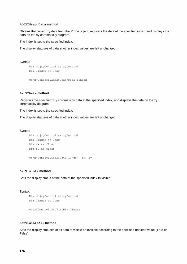
AddXYGraphData method
Obtains the current xy data from the Probe object, registers the data at the specified index, and displays the data on the xy chromaticity diagram.
The index is set to the specified index.
The display statuses of data at other index values are left unchanged.
Syntax: Dim objxyControl as xyControl
Dim lIndex as long
ObjxyControl.AddXYGraphData lIndex
SetXYData method
Registers the specified x, y chromaticity data at the specified index, and displays the data on the xy chromaticity diagram.
The index is set to the specified index.
The display statuses of data at other index values are left unchanged.
Syntax: Dim objxyControl as xyControl
Dim lIndex as long
Dim fx as float
Dim fy as float
ObjxyControl.SetXYData lIndex, fx, fy
SetVisible method
Sets the display status of the data at the specified index to visible.
Syntax: Dim objxyControl as xyControl
Dim lIndex as long
ObjxyControl.SetVisible lIndex
SetVisibleAll method
Sets the display statuses of all data to visible or invisible according to the specified boolean value (True or False).
176

Syntax: Dim objxyControl as xyControl
Dim bVisible as Boolean
ObjxyControl.SetVisibleAll bVisible
ClearData method
Clears all data registered on the control and initializes the index.
Syntax: Dim objxyControl as xyControl
ObjxyControl.ClearData
177

4-3-2-2: xyControl: Using in VB
Add the CA-SDK component xyControl to the VB project as described in section 4-3-1-2: CaControl: Using in VB .
The source code shown below is extracted from the CA-SDK Color measurement sample software.
After creating the SDK object, the objects for controlling the CA unit are set on the control using the control's properties ( , ). (The control has been placed on the FormMeasurement form.)
Then, the control is initialized using ClearData.
After performing the above procedure, the control is ready to be used.
In the CA-SDK sample software, when a measurement is taken the measurement results are plotted on the xy chromaticity diagram. This is performed using SetXYGraphData. SetXYGraphData sets only the latest data to visible; previous measurement data are not displayed.
In addition, the measurement results in the sample software are stored in a grid control, and when the user selects data rows in the control, the xy chromaticity data for the selected rows in the control are plotted on the chromaticity diagram. This is performed in and in the source code. First, SetVisibleAll is used with the parameter set to FALSE to set the display statuses for all data to invisible. Then, the display statuses for the data selected in the grid control are set to visible using SetVisible.
Ca200Sample.bas Public Sub Main()
...
Set objCa200 = New Ca200
...
objCa200.AutoConnect
...
Set objCa = objCa200.SingleCa
Set objProbe = objCa.SingleProbe
Set objMemory = objCa.Memory
...
Set FormMeasurement.xyControl1.Probe = objProbe
Set FormMeasurement.xyControl1.Ca = objCa
...
FormMeasurement.frm Sub GridInit()
...
xyControl1.ClearData
...
End Sub
178

Sub SetSingleData(ByVal LisNo As Integer)
...
xyControl1.SetXYGraphData
...
End Sub
Private Sub grdDataList_MouseUp(Button As Integer, Shift As Integer, X As ...
xyControl1.SetVisibleAll False
lSelectedRow1 = grdDataList.MouseRow
If lSelectedRow0 > lSelectedRow1 Then
For L = lSelectedRow1 To lSelectedRow0
If L <= ListNo Then
xyControl1.SetVisible L
Else
Exit Sub
End If
Next L
Else
For L = lSelectedRow0 To lSelectedRow1
If L <= ListNo Then
xyControl1.SetVisible L
Else
Exit Sub
End If
Next L
End If
End Sub
179

4-3-2-3: xyControl: Using in VC++ (MFC)
The sample software is a dialog-based application with the GUI shown in section 4-3-2: xyControl (for Displaying Data in xy Color Space) .
First, the CA-SDK component xyControl should be added to the project. Please see section 4-3-1-3: CaControl: Using in VC++ (MFC) for information on doing this.
• If the project is built at this point, an error indicating that the SetChannelID() method of the IMemory class defined in the file "ca200Srvr.h" created automatically by the tool is defined twice will appear. This is because for the ChannelID property of the CA-SDK Memory object, the name of the settings wrapper method created automatically by the tool (SetChannelID) is colliding with the name of the SetChannelID method originally provided for the Memory object. It is therefore necessary to change one of the names. In the sample software, the name of the original method has been changed to SetID.
Place the control and the Measure button on the main window to create the GUI.
Then, the following must be performed to complete coding preparations: 1 Add the control class DDX member variable m_CxyControl to the dialog class. 2 Add the CA-SDK object class member variables m_ICa200, m_ICa, and m_IProbe to the dialog class. 3 Add the OnMsr handler for the Measure button to the dialog class.
In the sample software, when the Measure button is pressed, a color measurement is taken and the x, y values of the measurement results are plotted on the xyControl.
Source code from the sample software for using the control is shown below.
The Ca200 object is created.
The Ca object is obtained (from the SingleCa property) using the GetSingleCa method.
An instance of the wrapper class ICa for the Ca object is attached. Thereafter, the ICa instance is manipulated in the same way as a Ca object.
In the same way, the setting for the Probe object is also performed. The code up to this point performs initialization of the CA-SDK objects.
Then, the Ca object and the Probe object are set in the xyControl using SetRefCa() and SetRefProbe().
Finally, the xyControl data are initialized using ClearData().
This makes the control ready to use.
The measurement and display section is in the OnMsr click handler of the Measure button.
180

In the source code list below, measurement is performed using MeasureRef of the Ca object. Then, the measurement data are obtained, registered in the control, and displayed using AddXYGraphData() of the xyControl. Since AddXYGraphData() simply adds data to the plot, the previously plotted measurement results remain shown on the plot.
Test2Dlg.cppBOOL CTest2Dlg::OnInitDialog()
{
...
// TODO: Add extra initialization here
m_ICa200.CreateDispatch("CA200Srvr.Ca200.1");
m_ICa200.m_bAutoRelease = TRUE;
m_ICa200.AutoConnect();
LPDISPATCH pICa = m_ICa200.GetSingleCa();
m_ICa.AttachDispatch(pICa);
LPDISPATCH pIProbe = m_ICa.GetSingleProbe();
m_IProbe.AttachDispatch(pIProbe);
...
m_ICa.CalZero();
m_CxyControl.SetRefCa(&m_ICa.m_lpDispatch);
m_CxyControl.SetRefProbe(&m_IProbe.m_lpDispatch);
m_CxyControl.ClearData();
m_lIndex = 0;
return TRUE; // return TRUE unless you set the focus to a control
}
void CTest2Dlg::OnMsr()
{
// TODO: Add your control notification handler code here
m_ICa.Measure(0);
m_CxyControl.AddXYGraphData(&m_lIndex);
m_lIndex++;
}
181

4-4: CA-SDK VB Sample Software
Several VB sample applications are included in the CA-SDK, along with the entire source code for these samples. Although the use of the CA-SDK objects is slightly different between VB and VC++, the source code for the VB samples should be a good reference when creating C++ applications using the CA-SDK.
182

4-4-1: Color/Flicker Measurement
Folder: ...CA-SDK\Sample\Color
This VB sample software measures color and flicker.
Creation and initialization of the CA-SDK objects is performed in the Main() procedure of the Ca200Sample.bas module. The VB sample software was written for the following conditions:
� Number of CA units: 1
� Number of probes: 1
� Connection: USB
Under such conditions, setting and initialization of the structures is simple, as shown in the code below ( ).
In the code below:
Creates the Ca200 object of the CA-SDK.
Sets the structure of the Ca200 object using the AutoConnect() method of the Ca200 object.
Obtains the connected Ca object from the SingleCa property of the Ca200 object.
Obtains the connected Probe object from the SingleProbe property of the Ca object.
Obtains the Memory channel object from the Memory property of the Ca object.
Obtains the CA instrument type from the CAType property of the Ca object.
Performs zero calibration using the CalZero() method of the Ca object.
Obtains the measuring probe ID and reference color setting values using the GetReferenceColor() method of the Memory object.
Ca200Sample.bas Public Sub Main()
Dim i As Integer
'===================================
' Set Error Trap
'===================================
On Error GoTo E
'===================================
' Create SDK/Application Object
'===================================
Set objCa200 = New Ca200
'===================================
183

' Set Configuration
'===================================
objCa200.AutoConnect
'===================================
' Initialize SDK Object
'===================================
Set objCa = objCa200.SingleCa
Set objProbe = objCa.SingleProbe
Set objMemory = objCa.Memory
CA_Type = objCa.CAType
...
'===================================
' Initialize CA and Application
'===================================
' 0 Calibration
MsgBox "0-Cal", vbOKOnly
objCa.CalZero
Screen.MousePointer = vbHourglass
objMemory.GetReferenceColor objProbe.ID, typCurrentRefereceData.sRefx, typCurrentRefereceData.sRefy, typCurrentRefereceData.sRefLv
...
End Sub
Measurement procedure samples for color measurement, JEITA flicker measurement, and FMA flicker measurement are all included in the SingleMeasure() procedure of the FormMeasurement.frm module. In all cases, in the code,
Performs measurement using the Measure() method of the Ca object.
Obtains the measurement result status and measurement values from the Probe object properties.
What type of measurement (color, JEITA flicker, FMA flicker) will be taken by the Measure() method depends on the setting of the DisplayMode property of the Ca object.
When JEITA flicker measurement is performed, the frequency component i used as the argument for the GetSpectrum(i) method of the Probe object can be obtained. ( ).
FormMeasurement.frm Private Sub SingleMeasure()
Dim i As Integer
On Error Resume Next
Select Case SelectDataName
Case "COLOR"
'===================================
184

' Color Measurement
'===================================
objCa.Measure
typCurrentMeasurementData.dateColorData = Date
typCurrentMeasurementData.timeColorData = Time
typCurrentMeasurementData.lColorStatus = objProbe.RD
typCurrentMeasurementData.ssx = objProbe.Sx
typCurrentMeasurementData.ssy = objProbe.Sy
typCurrentMeasurementData.sLv = objProbe.Lv
typCurrentMeasurementData.sLvfL = objProbe.LvfL
typCurrentMeasurementData.Sx = objProbe.X
typCurrentMeasurementData.Sy = objProbe.Y
typCurrentMeasurementData.Sz = objProbe.Z
typCurrentMeasurementData.sud = objProbe.ud
typCurrentMeasurementData.svd = objProbe.vd
typCurrentMeasurementData.sduv = objProbe.duv
typCurrentMeasurementData.LT = objProbe.T
Case "FMA"
'===================================
' FMA Measurement
'===================================
objCa.Measure
typCurrentMeasurementData.dateFMAData = Date
typCurrentMeasurementData.timeFMAData = Time
typCurrentMeasurementData.lFMAStatus = objProbe.RFMA
typCurrentMeasurementData.sFMA = objProbe.FlckrFMA
Case "JEITA"
'===================================
' JEITA Measurement
'===================================
objCa.Measure
typCurrentMeasurementData.dateJEITAData = Date
typCurrentMeasurementData.timeJEITAData = Time
typCurrentMeasurementData.lJEITAStatus = objProbe.RJEITA
typCurrentMeasurementData.sJEITA = objProbe.FlckrJEITA
SpectMin = 0
SpectMax = -100
For i = 6 To 65
typCurrentMeasurementData.Gspect(i) = objProbe.GetSpectrum(i)
If typCurrentMeasurementData.Gspect(i) <> -999 Then
If SpectMin > typCurrentMeasurementData.Gspect(i) Then
SpectMin = typCurrentMeasurementData.Gspect(i)
End If
If SpectMax < typCurrentMeasurementData.Gspect(i) Then
SpectMax = typCurrentMeasurementData.Gspect(i)
End If
End If
185

Next i
End Select
SetCurrentData
End Sub
186
4-4-2: Gamma Measurement
Folder: ...CA-SDK\Sample\Gamma
This VB sample software measures gamma characteristics.
Gamma measurement is performed in the MeasureGamma() procedure of the FormGamma.frm module. The video generator is controlled and the input/output characteristics and gradation characteristics of white and RGB are measured.
187

4-4-3: Contrast Measurement
Folder: ...CA-SDK\Sample\Contrast
This VB sample software measures contrast and uniformity.
Contrast and uniformity measurements are performed in the MeasureUniformity() procedure of the FormContrast.frm module.
188

4-4-4: Calibration
Folder: ...CA-SDK\Sample\Cal
This VB sample performs calibration of the CA unit.
In this calibration software, first the calibration data for all channels is read from the unit and displayed. This is performed in the Form_Activate() procedure of the FormCaCal.frm module. In this procedure, the information for each memory channel on the unit is obtained and displayed as follows:
Sets the memory channel number in the ChannelNO property of the Memory object.
Obtains the serial number of the currently connected probe, the serial number of the probe used for calibration, the serial number of the probe used for setting the reference color, and the calibration mode (white/matrix) using the GetMemoryStatus() method of the Memory object.
Obtains the serial number of the connected probe and the set reference color values using the GetReferenceColor() method of the Memory object.
FormCaCal.frm Private Sub Form_Activate()
...
Dim i As Integer
For i = 1 To 100
DoEvents
With atypCaCalInfo(i)
objMemory.ChannelNO = i - 1
objMemory.GetMemoryStatus objProbe.Number, .lCalProbeSNO, .lRefProbeSNO, .lCalMode
objMemory.GetReferenceColor objProbe.ID, .sRefx, .sRefy, .sRefLv
...
End With
Next i
...
End Sub
Calibration is performed in the CommandCal_Click() procedure of the FormCaCal.frm module. The procedure is broken into several blocks separated by comments.
The block following the comment 'UserCal performs matrix calibration.
The block following the comment 'White Cal performs white calibration.
The block following the comment 'White Set sets the reference color to the measured values.
189

The block following the comment 'White Data Set sets the numerical values for CH00 as the reference color.
Except for setting the reference color to the measured values, all other calibration and reference color setting processes require that the necessary calibration or reference color x, y, Lv values be set in advance. In addition, the probe for which the ID has been set in the DisplayProbe property of the Ca object will be the probe which is used.
In matrix calibration, the following is performed:
Sets the calibration channel number in the ChannelNO property of the Memory object.
Sets the calibration mode using the SetLvxyCalMode() method of the Ca object.
Then, for each calibration image (R, G, B, White):
Measures the calibration image using the Measure() method of the Ca object.
Sets the calibration values using the SetLvxyCalData() method of the Ca object.
After to have been performed for R, G, B, and White:
Performs Enter() method of Ca object.
For white calibration, the above process is performed for only the White calibration image.
For setting a reference color, and are performed for the White calibration image.
For setting the reference color for CH00, only is performed.
FormCaCal.frm Private Sub CommandCal_Click()
...
'================================
' UserCal
'================================
objCa.DisplayMode = DSP_LXY
objMemory.ChannelNO = ListNo - 1
objCa.SetLvxyCalMode
bSetMode = True
'--------------------------------
' Red
'--------------------------------
Result = MsgBox("Red Measure", vbOKCancel)
If Result = vbCancel Then
objCa.ResetLvxyCalMode
Exit Sub
End If
objCa.Measure
190

objCa.SetLvxyCalData CLR_RED, typCalData(CLR_RED).sRefx, typCalData(CLR_RED).sRefy, typCalData(CLR_RED).sRefLv
'--------------------------------
'Green
'--------------------------------
Result = MsgBox("Measure Green", vbOKCancel)
If Result = vbCancel Then
objCa.ResetLvxyCalMode
Exit Sub
End If
objCa.Measure
objCa.SetLvxyCalData CLR_GREEN, typCalData(CLR_GREEN).sRefx, typCalData(CLR_GREEN).sRefy, typCalData(CLR_GREEN).sRefLv
'--------------------------------
'Blue
'--------------------------------
Result = MsgBox("Measure Blue", vbOKCancel)
If Result = vbCancel Then
objCa.ResetLvxyCalMode
Exit Sub
End If
objCa.Measure
objCa.SetLvxyCalData CLR_BLUE, typCalData(CLR_BLUE).sRefx, typCalData(CLR_BLUE).sRefy, typCalData(CLR_BLUE).sRefLv
'--------------------------------
'White
'--------------------------------
Result = MsgBox("Measure White", vbOKCancel)
If Result = vbCancel Then
objCa.ResetLvxyCalMode
Exit Sub
End If
objCa.Measure
objCa.SetLvxyCalData CLR_WHITE, typCalData(CLR_WHITE).sRefx, typCalData(CLR_WHITE).sRefy, typCalData(CLR_WHITE).sRefLv
objCa.Enter
ElseIf OptionRefCal.Value = True Then
If objMemory.ChannelNO = 0 Then
MsgBox "CH00 cannot be calibrated", vbOKOnly
Exit Sub
End If
191

'================================
' White Cal
'================================
objCa.DisplayMode = DSP_LXY
objMemory.ChannelNO = ListNo - 1
objCa.SetLvxyCalMode
bSetMode = True
'--------------------------------
'White
'--------------------------------
Result = MsgBox("Measure White", vbOKCancel)
If Result = vbCancel Then
objCa.ResetLvxyCalMode
Exit Sub
End If
objCa.Measure
objCa.SetLvxyCalData CLR_WHITE, typCalData(CLR_WHITE).sRefx, typCalData(CLR_WHITE).sRefy, typCalData(CLR_WHITE).sRefLv
objCa.Enter
ElseIf OptionRefSet.Value = True Then
'================================
' White Set
'================================
If objMemory.ChannelNO = 0 Then
MsgBox "CH00 cannot be set", vbOKOnly
Exit Sub
End If
objCa.DisplayMode = DSP_LXY
objMemory.ChannelNO = ListNo - 1
Result = MsgBox("White Measure", vbOKCancel)
If Result = vbCancel Then
Exit Sub
End If
objCa.Measure
objCa.Enter
ElseIf OptionRefData.Value = True Then
'================================
' White Data Set(CH00)
'================================
If objMemory.ChannelNO <> 0 Then
MsgBox "Only For CH00", vbOKOnly
Exit Sub
End If
objCa.SetLvxyCalData CLR_WHITE, typCalData(CLR_WHITE).sRefx,
192

typCalData(CLR_WHITE).sRefy, typCalData(CLR_WHITE).sRefLv
Else
...
End Sub
193
4-5: Creating a Visual Basic .NET Application using the CA-SDK
Visual Basic .NET (VB.NET) is the new application development/execution environment from Microsoft (hereinafter referred to as "MS"). There is also a .NET version of Visual Studio (VS), MS's Integrated Development Environment (IDE), and it is this IDE that should be used to create the program when developing a CA-SDK application in VB.NET. The CA-SDK will be implemented as a component using COM.
In the previous version of Visual Basic (VB), a simple application could be written by just setting the references to the COM component.
In VB.NET, although the specifications have changed greatly, by using the IDE it is possible to perform development as with the previous VB.
In this section, we will explain how to create a CA-SDK application program using VB.NET. (In this explanation, we will use Visual Studio .NET 2003. Other versions may have screens somewhat different than those used here.)
Creation of an application consists of the following processes: 1 Installing the CA-SDK. 2 Creating a VB.NET project in the IDE. 3 Setting the references to the CA-SDK. 4 Creating the application GUI and code.
Before beginning to work in VB.NET, perform step 1: Installing the CA-SDK. For the CA-SDK installation procedure, please refer to the CA-SDK instruction manual.
The explanation that follows is for "Step 2: Creating a VB.NET project in the IDE", and the remaining steps.
194

4-5-1: Creating the VB.NET project
1 In the Start screen of VS, select "Create New Project" (or select "File" from the menu, then "Create New", and then "Project"). The New Project dialog will appear
2 In the New Project dialog, select "Visual Basic" as the project type, and "Windows Application" as the template to use. Type "Ca200Sample" as the project location and as the project name for the sample software, and click OK.
The project will be created and the form design screen will appear, as shown on the next page.
195

196

4-5-2: Setting references to CA_SDK
1 Right-click on "References" in the Solution Explorer, and select "Add Reference..." from the pop-up menu which appears (or select "Project" from the menu and then select "Add Reference..."). The Add Reference dialog will appear.
2 In the Add Reference dialog, select the COM tab and select the component name "CA200Srvr" in the upper list, and then click the "Select" button. CA200Srvr will be added to the Selected Components list. Click OK to close the dialog.
197

The .NET assembly (.NET component) CA200SRVRLib for using the CA-SDK will be automatically created from the CA-SDK's type library by the IDE, and the reference settings will be added. This enables the CA-SDK to be used by the application.
198
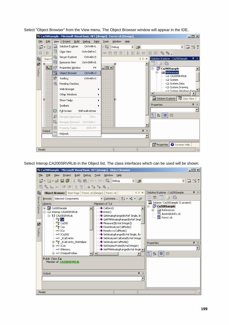
Select "Object Browser" from the View menu. The Object Browser window will appear in the IDE.
Select Interop.CA200SRVRLib in the Object list. The class interfaces which can be used will be shown.
199

4-5-3: Creation of Application GUI/Code
The UI (user interface) will be as shown below. There are a total of 10 static text controls (5 as labels and 5 for displaying measurement data) and 3 push buttons.
• When the Zero Cal button is pressed, zero calibration is performed by the CA instrument. • When the Measure button is pressed, a series of 20 measurements are taken and the measurement
results are shown in the main window after each measurement. • When the Cancel button is pressed, the series of measurements is interrupted and canceled.
The GUI is created by selecting items in the toolbox and positioning them on the form, as in the previous version of VB. If the toolbox is not shown, select "Toolbox" from the "View" menu. Then the toolbox will appear when the mouse cursor is positioned over the Toolbox icon in the toolbar at the upper left of the design window.
200

As with the previous version of VB, set the properties of each control to design the GUI.
201

The required code is also almost the same as for the previous version of VB.
An explanation of the sample software code follows.
1 Declaring the CA-SDK public class members
VB.NET is a true object-oriented language, and the basic unit for program construction is the class.
In the sample source code, declares the CA-SDK .NET class member as a custom property of the Form1 class. adds the WithEvents keyword to the Ca class member, as with the previous version of VB. This enables the event handler for the CA-SDK public members to be written.
Declarations for each of the controls on Form1 are included in the code created by the Windows form designer.
2 Creating the event handlers
The event handlers for when each of the buttons are clicked will now be written. This is performed in the same way as for the previous version of VB, by selecting the button for which the event handler will be written in the Class Name box above the code editing window, selecting the event to be handled in the Event Name box, and then adding the necessary code to the event handler definition which will be automatically created.
202

The public events for the CA-SDK are written in the same way. Select the Ca class member variables from the Class Name box (for the sample software, select objCa), and then select ExeCalZero in the Event Name box, and add the necessary code to the definition for the objCa_ExeCalZero() handler which is automatically created. This handler will be executed in response to the event fired from the CA-SDK when the probe temperature changes more than a certain value.
In the Load event for Form1 in the sample software, the CA-SDK Ca200 object is created and the structure settings are made , and thereafter the CA-SDK object to be used by the application is obtained.
In the Click event of ButtonMeasure (the Measure button control), measurement is performed by the CA-SDK Ca object, and the measurement results are obtained by the Probe object and displayed by the labels.
In the Click event of ButtonCalZero (the Cal Zero button) , or in response to the ExeCalZero event of the CA-SDK , the Ca object performs zero calibration.
In the Closing event which is fired when the close button of the form is clicked, the Ca object is set to Remote Off . (The Closing event can be selected in the Event Box when Base Class Events is selected in the Class Name box.)
3 Error Handling
In VB.NET, error handling code can be written in the same way as for the previous version of VB , . In addition, structured exception handling can also be written .
203

As can be seen from the sample software code, operation using the CA-SDK objects in VB.NET is virtually the same as when using the previous version of VB.
However, as was described somewhat in this explanation, the substance of VB.NET is greatly different from the previous version of VB, so that it could be said to be an entirely different language. By using the new functions offered by VB.NET, applications more complicated than before can be easily and efficiently developed.
Public Class Form1
Inherits System.Windows.Forms.Form
#Region " Windows Form Designer generated code "
(Abbreviated)
#End Region
Private objCa200 As CA200SRVRLib.Ca200Class
Private WithEvents objCa As CA200SRVRLib.CaClass
Private objProbe As CA200SRVRLib.ProbeClass
Private isMsr As Boolean
Private Sub Form1_Load(ByVal sender As System.Object, ByVal e As
System.EventArgs) Handles MyBase.Load
On Error GoTo er
objCa200 = New CA200SRVRLib.Ca200Class()
objCa200.AutoConnect()
objCa = objCa200.SingleCa
objProbe = objCa.SingleProbe
Exit Sub
er:
DspError()
End
End Sub
Private Sub ButtonCancel_Click(ByVal sender As System.Object, ByVal e
As System.EventArgs) Handles ButtonCancel.Click
isMsr = False
ButtonCancel.Enabled = False
ButtonMeasure.Enabled = True
ButtonCalZero.Enabled = True
End Sub
204

Private Sub ButtonMeasure_Click(ByVal sender As System.Object, ByVal e
As System.EventArgs) Handles ButtonMeasure.Click
Dim i As Integer
On Error GoTo er
isMsr = True
ButtonCancel.Enabled = True
ButtonMeasure.Enabled = False
ButtonCalZero.Enabled = False
For i = 1 To 20
objCa.Measure()
LabelLv.Text = objProbe.Lv.ToString("###.##")
Labelx.Text = objProbe.sx.ToString("#.####")
Labely.Text = objProbe.sy.ToString("#.####")
LabelT.Text = objProbe.T.ToString("####")
Labelduv.Text = objProbe.duv.ToString("#.####")
Application.DoEvents()
If isMsr = False Then
ButtonCancel.Enabled = False
ButtonMeasure.Enabled = True
Exit Sub
End If
Next
ButtonCancel.Enabled = False
ButtonMeasure.Enabled = True
ButtonCalZero.Enabled = True
Exit Sub
er:
DspError()
End
End Sub
Private Sub ButtonCalZero_Click(ByVal sender As System.Object, ByVal e
As System.EventArgs) Handles ButtonCalZero.Click
retry:
ButtonMeasure.Enabled = False
ButtonCalZero.Enabled = False
Try
objCa.CalZero()
Catch er As Exception
If MessageBox.Show("Zero Cal Error" + Chr(13) + "Retry?",
"CalZero", MessageBoxButtons.OKCancel) = DialogResult.Cancel
Then
objCa.RemoteMode = 0
205

End
End If
GoTo retry
End Try
ButtonMeasure.Enabled = True
ButtonCalZero.Enabled = True
End Sub
Private Sub objCa_ExeCalZero() Handles objCa.ExeCalZero
If MessageBox.Show("CalZero?", "CalZero",
MessageBoxButtons.OKCancel) = DialogResult.Cancel Then
Exit Sub
End If
ButtonMeasure.Enabled = False
ButtonCalZero.Enabled = False
retry:
Try
objCa.CalZero()
Catch er As Exception
MessageBox.Show("Zero Cal Error!" + Chr(13))
GoTo retry
End Try
ButtonMeasure.Enabled = True
ButtonCalZero.Enabled = True
End Sub
Private Sub DspError()
Dim msg As String
msg = "Error from" + Err.Source + Chr(10) + Chr(13)
msg = msg + Err.Description + Chr(10) + Chr(13)
msg = msg + "HR:" + (Err.Number - vbObjectError).ToString
MessageBox.Show(msg)
End Sub
Private Sub Form1_Closing(ByVal sender As Object, ByVal e As
System.ComponentModel.CancelEventArgs) Handles MyBase.Closing
objCa.RemoteMode = 0
End Sub
End Class
206

5: Application Examples 5-1: CA-210 Application Example (White Balance Adjustment System)
5-1-1: White Balance Adjustment
When white is displayed on several units of LCD monitors, the colors shown on the displays may appear to be different. This is due to variations in the components (filters, circuits, etc.) which causes the white to not appear to be exactly the same color.
For example, if there was a 0.02 difference in the x, y chromaticity due to component variations, the colors would be as shown below.
x=0.310, y=0.332, Lv=172.5
Target chromaticity and luminance
x=0.292, y=0.356, Lv=170.3
Unadjusted chromaticity and luminance
On the other hand, recently the use of LCD monitors for viewing images has increased, and demands for more accurate chromaticity and luminance reproduction is also increasing. In order to reduce variations in the displayed color, cases where white balance adjustment of LCD monitors is performed have been increasing.
207

x=0.315, y=0.337, Lv=169.4
Chromaticity and luminance after adjustment
An example of a system using the CA-210 for high-speed, high-accuracy adjustment of the luminance and chromaticity of white and inspection of contrast will be explained in the following sections.
208

5-1-2: System Block Diagram (White Balance Adjustment)
CA-210 + 1 probe For measuring luminance and chromaticity
UUT (Unit Under Test)
The LCD monitor to be adjusted. The type to which calibration data can be written from an external device. In this example, communication is performed using RS-232C.
PC Computer to control the measuring instrument, LCD monitor, and pattern generator
USB port x 1 (for CA-210)
RS-232C port x 2 (1 for controlling LCD and 1 for controlling VG)
Pentium III 660MHz or faster
Resolution: XGA
VG-823, 813, 812 Used for controlling the pattern displayed on the UUT. Pattern generator manufactured by Astrodesign Inc.
Note: If I2C is used, an RS-232C to I2C converter is necessary.
209

5-1-3: White Balance Adjustment Software Functions
• Varies the gain of the LCD monitor to adjust it so that the color displayed on the monitor matches the specified chromaticity and luminance. Up to 6 types of settings can be performed in sequence.
• Inspects the contrast.
• Has pass/fail judgment function.
210

5-1-4: White Balance Adjustment Time
The white balance adjustment time varies depending on the required adjustment accuracy.
For luminance accuracy of:
And chromaticity accuracy of:
Adjustment time would be
±10 ±0.01 Within 5 sec.
±5 ±0.005 Within 10 sec.
• Operating environment: Fujitsu FMV-6600MF8/X PIII 660MHz; memory: 128MB
211
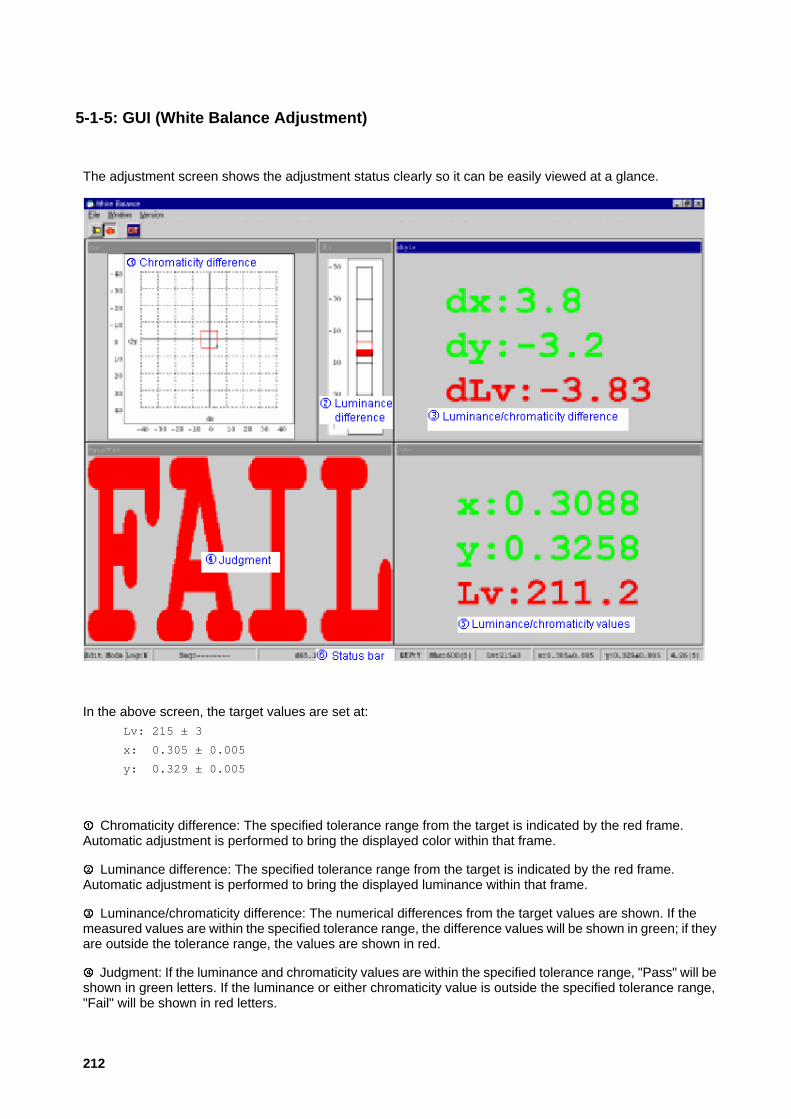
5-1-5: GUI (White Balance Adjustment)
The adjustment screen shows the adjustment status clearly so it can be easily viewed at a glance.
In the above screen, the target values are set at: Lv: 215 ± 3
x: 0.305 ± 0.005
y: 0.329 ± 0.005
Chromaticity difference: The specified tolerance range from the target is indicated by the red frame. Automatic adjustment is performed to bring the displayed color within that frame.
Luminance difference: The specified tolerance range from the target is indicated by the red frame. Automatic adjustment is performed to bring the displayed luminance within that frame.
Luminance/chromaticity difference: The numerical differences from the target values are shown. If the measured values are within the specified tolerance range, the difference values will be shown in green; if they are outside the tolerance range, the values are shown in red.
Judgment: If the luminance and chromaticity values are within the specified tolerance range, "Pass" will be shown in green letters. If the luminance or either chromaticity value is outside the specified tolerance range, "Fail" will be shown in red letters.
212

Luminance/chromaticity measurement values: The numerical measurement values are shown. If the measurement values are within the specified tolerance range, the values will be shown in green; if they are outside the tolerance range, the values are shown in red.
Status bar: Shows various settings including the target luminance and chromaticity values and the adjustment time.
When the CA-210 is used as described above, high-speed, high-accuracy white balance adjustment can be performed.
213

5-2: CA-210 Application Example (Gamma Adjustment System)
5-2-1: Gamma Adjustment
When multiple LCD monitors display the same image, the midtones may appear to be different. This is due to variations in the components (filters, circuits, etc.) which causes the midtones to not appear to be exactly the same colors.
For example, if the brightness of the midtones varied due to component variations, the images on the LCD monitors might be as shown below.
On the other hand, recently the use of LCD monitors for viewing images has increased, and demands for more accurate midtone reproduction is also increasing. In order to reduce variations in the displayed color, cases where adjustment of LCD monitors is performed have been increasing.
An example of a system using the CA-210 for high-speed, high-accuracy adjustment of midtone balance for each primary color will be explained in the following sections.
214

5-2-2: System Block Diagram (Gamma Adjustment)
CA-210 + 1 probe For measuring luminance and chromaticity
UUT (Unit Under Test)
The LCD monitor to be adjusted. The type to which calibration data can be written from an external device. In this example, communication is performed using RS-232C.
PC Computer to control the measuring instrument, and LCD monitor
USB port x 1 (for CA-210)
RS-232C port x 1 (for controlling LCD)
Pentium III 660MHz or faster
Resolution: XGA, True Color (24-bit or higher)
Graphic board Specified graphic board capable of displaying True Color (24-bit or higher)
Note: If I2C is used, an RS-232C to I2C converter is necessary.
215

5-2-3: Gamma Adjustment Process
The patterns displayed on the unit under test are output by the PC's graphics board. Set the PC to display multiple windows, and let the PC display the software and also have the graphic card display the test pattern.
The method for measuring characteristics is as specified in IEC61966-4, where gamma is calculated from tristimulus values.
Specifically, the X values for red, the Y values for green, and the Z values for blue are normalized using the maximum values for each color.
measurement
First, the current characteristics of the LCD are measured at several steps. (number of steps: 8, 16, 32, 64, 128, and 256)
An example of the results is shown at right.
Horizontal axis: Steps 0 to 255
Vertical axis: Measured values for each color normalized using the maximum values for each color.
Setting of value.
The characteristics are set.
In the example at right, is set to 2.2.
The setting data are calculated for each step using the equation curve = (step) x 2.2
An LUT (Look Up Table) of the setting data used in the example at right is calculated from the data measured in , and this LUT is written to the LCD monitor.
The calculation method for the LUT is as follows:
For example, for step 16, where the data calculated as (16^2.2)/(255^2.2) (= Value/Max. value) is located in the measurement data would be determined, and the LUT value would then be determined by linear interpolation using the point above and the point below this point.
216

inspection
The LCD to which the LUT has been written is then measured again to verify that the LUT data has been accurately reflected in the display.
An example is shown at right.
217

5-2-4: Gamma Adjustment Time
The time for adjusting the characteristics of the 3 colors R, G, and B is shown in Table 1 below.
Note: A 100ms wait is provided to allow the LCD response to stabilize after the displayed pattern has been changed. The times listed do not include the time to write the LUT to the LCD monitor.
Operating environment: Fujitsu FMV-6600MF8/X PIII 660MHz; Memory: 128MB
Num ber of s teps 8 16 32 64 128 256Adjus tm ent tim e 6 8 12 19 34 64
Table 1: γ adjus tm ent tim e (sec.)
When the CA-210 is used as described in this section, high-speed, high-accuracy adjustment of characteristics from low to high luminance can be performed, so that midtones can be correctly reproduced.
218

5-2-5: GUI (Gamma Adjustment)
Adjustment display screen examples
The focus is on displaying the condition at the time of measurement.
measurement screen
The LCD monitor's characteristics are measured at the specified measurement steps and the results are displayed.
LUT setting display screen
The setting data which will be written to the LCD monitor are displayed. In this example, the values are set to 2.1 for R. 2.2 for G, and 2.3 for B.
verfication screen
The LCD monitor to which the LUT was written is measured again, and the resulting
characteristics are displayed.
In addition, any desired image can also be displayed to check the results.
219

6: Related Standards 6-1: CA-210 and ED-2522 Standards
6-1-1: Introduction
The three most well-known standards defining the methods for measuring LCD panels are:
• ED-2522 issued by the Japan Electronics and Information Technology Industries Association (JEITA)
• Flat Panel Display Measurements Standard issued by the Video Electronics Standards Association (VESA)
• IEC61966-4 issued by the International Electrotechnical Commission (IEC)
In addition, ISO-13406 from the International Standards Organization is a standard from the human engineering viewpoint.
This section will provide an overview of the ED-2522 standard, as well as how the CA-210 relates to the measurement methods defined in the standard. (Note 6-1-1)
Notes
Note 6-1-1:
Currently, discussions are underway regarding the international standard IEC 61747-6 based on the ED-2522 standard.
220

6-1-2: Measurement Items
The measurement items specified in ED-2522 (JEITA) are the 14 items listed in Table 6-1-1 below:
Measurement ItemContrast ratio measurement methodResponse time measurement method
X Module component block current consumption or power consumption measurement methodWhite chromaticity measurement methodColor reproduction range measurement methodVertical field of view measurement methodHorizontal field of view measurement methodViewing direction without gray-scale inversionLuminance and luminance non-uniformity measurement methodLuminance warmup characteristics measurement method
X Resolution measurement methodCrosstalk measurement methodFlicker measurement method (See Note 1.)Specular reflectance ratio measurement method
Table 6-1-1: ED-2522 measurement items
In the table above, the items marked with are the items which should be measured with a colorimeter (luminance meter). (See section 1-2: About Color-Measuring Instruments.)
221

6-1-3: Measurement Items and CA-210
Considering the characteristics of colorimeters, there are some items that the colorimeter is not suitable for measuring. The following performance specifications determine whether or not a colorimeter is suitable:
• High-accuracy measurement of white (luminance, chromaticity)
• High-accuracy measurement of primary colors (luminance, chromaticity)
• High-accuracy measurement at low luminance (See Note 6-1-2.)
• Measurement distance, large depth of field (no obstruction even if the LCD is tilted)
• ms-order measurement tracking
• Multi-point measurement capability
Table 6-1-2 shows the relationship between these performance specifications and the measurement items which should be measured using a colorimeter. In Table 6-1-2, a indicates that a colorimeter has the specifications required for measuring the measurement item. In particular, if the CA-210 is suitable for measuring the item or if it has the required specifications, the item or specification is colored blue; if the CA-210 is not suitable for measuring the item or does not have the required specifications, the item or specification is colored red. (The main specifications of the CA-210 are listed in Table 6-1-3.)
Measurement item
White lum
inance
Prim
ary color
Low lum
inance
Distance
ms tracking
Response time
Vertical field of viewHorizontal field of viewViewing direction without gray-scale inversion
Specular reflectance ratio
Multi-point
Contrast ratio
White chromaticityColor reproduction range
Luminance and luminance non-uniformityLuminance warmup characteristicsCrosstalkFlicker (with CA-210 LCD Flicker Measuring Probe only)
Table 6-1-2: Relationship between colorimeter specifications and measurement items
222

x,y,Lv; u',v',Lv; T,∆uv,Lv; X,Y,Z; R,G,B; Flicker (Contrast method/JEITA method; available only with CA-210 LCD Flicker Measuring Probe)
Measurement range 0.1 to 1000cd/m2
Luminance ±2% ±1 digit (0.1 to 1000cd/m2)Chromaticity White: ±0.002; Primary color: ±0.004 (Standard LCD, 160cd/m2)
White: ±0.003 (Standard LCD, 20.0 to 1000cd/m2)Luminance 0.2% ±1 digit (0.1 to 0.99cd/m2)
0.1% ±1 digit (1.00 to 1000cd/m2)Chromaticity 0.001 (Standard LCD displaying white, 1.00 to 1000cd/m2)
20 times/sec.Ø27mm30mm ±10mm5°Multi-probe expansion function for measurement of up to 5 points
Table 6-1-3: Main specifications of CA-210
Measurement item
Measurement speedMeasurement areaMeasurement distanceAcceptance angleOther
Accuracy
Repeatability
For measurements of Contrast Ratio and Crosstalk, low-luminance measurements are indispensible. For measurement of the Color Reproduction Range, high-accuracy measurements of primary colors are necessary. The CA-210 has specifications that enable these items to be measured. When the Universal Measuring Probe is used, a total of 6 of the items listed in Table 6-1-2 (the blue items excluding Flicker) can be measured; when the Flicker Measuring Probe is used, a total of 7 of the items listed in Table 6-1-2 (the blue items) can be measured.
ED-2522 specifies that, when measuring a standard LCD with a colorimeter, the measurement area should include at least 500 dots. The CA-210 has a measurement area of Ø27mm, so it satisfies this requirement. In addition, its aiming function makes it easier to set the measuring position.
All of the measurement items listed in Table 6-1-2 should be carried out under darkroom conditions (illuminance of 1lx or less). Since a hood can be attached to the CA-210's measuring probe, it is much easier to achieve darkroom conditions.
In addition, since multiple points can be measured simultaneously, the CA-210 can provide higher efficiency for items requiring measurements of multiple points.
However, there are also some items for which the CA-210 is not suitable for measuring. For example, for measurements of Response Time, it is necessary to obtain output tracking the luminance changes at 1ms intervals, but the CA-210 does not have such a function. In addition, for measurements related to viewing angle (including measurements of specular reflection ratio), although measurements normal to the LCD screen can be performed, for sharp tilting of the display the measuring probe may become an obstruction (since the measuring distance is 30mm ±10mm), and it may be impossible to take measurements due to insufficient depth of field.
Notes
Note 6-1-2:
Since the minimum luminance which can be displayed by an LCD is approximately 0.5, the colorimeter must have a measurement range specification which extends to below this value.
223
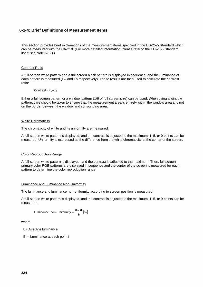
6-1-4: Brief Definitions of Measurement Items
This section provides brief explanations of the measurement items specified in the ED-2522 standard which can be measured with the CA-210. (For more detailed information, please refer to the ED-2522 standard itself; see Note 6-1-3.)
Contrast Ratio
A full-screen white pattern and a full-screen black pattern is displayed in sequence, and the luminance of each pattern is measured (Lw and Lb respectively). These results are then used to calculate the contrast ratio:
bw LL=Contrast
Either a full-screen pattern or a window pattern (1/6 of full screen size) can be used. When using a window pattern, care should be taken to ensure that the measurement area is entirely within the window area and not on the border between the window and surrounding area.
White Chromaticity
The chromaticity of white and its uniformity are measured.
A full-screen white pattern is displayed, and the contrast is adjusted to the maximum. 1, 5, or 9 points can be measured. Uniformity is expressed as the difference from the white chromaticity at the center of the screen.
Color Reproduction Range
A full-screen white pattern is displayed, and the contrast is adjusted to the maximum. Then, full-screen primary color RGB patterns are displayed in sequence and the center of the screen is measured for each pattern to determine the color reproduction range.
Luminance and Luminance Non-Uniformity
The luminance and luminance non-uniformity according to screen position is measured.
A full-screen white pattern is displayed, and the contrast is adjusted to the maximum. 1, 5, or 9 points can be measured.
[ ]%B
BB i−=uniformity-non Luminance
where
B= Average luminance
Bi = Luminance at each point i
224

Luminance Warmup Characteristics
With the display set to its maximum luminance, the luminance change over time is measured (from the time the display is switched on until the luminance sufficiently stable for several minutes). Be sure that the temperature of the display has sufficiently adjusted to the ambient temperature prior switching on the display. If it is also necessary to know the change at the edges of the display, multi-point measurement can be used.
Crosstalk
With a window pattern on the display, the drive signal is adjusted and set to the position at which crosstalk is at a maximum. Under these conditions, the background luminance (Lb), window luminance (Lw), and crosstalk luminance (Li) are measured Crosstalk is then calculated as:
[ ]%wb
ibLLLL
−
−=Crosstalk
(Crosstalk is the phenomenon in which the luminance and chromaticity of the pattern shown in one area of the screen affects the luminance and chromaticity of the pattern shown in a different area of the screen.)
Flicker
The luminance variation when flicker occurs is measured, and after the frequency components have been determined, the flicker value is calculated from the power spectrum of the DC component (P0) and the maximum power spectrum of the frequency components (Px) using the equation:
[ ]dBPPX ⎟
⎠⎞
⎜⎝⎛•=
0log10value Flicker
The result is luminance variation characteristics that include the influence of the frequency response characteristics of the human eye.
(See section 1-7-2-1: Flicker Measurement.)
Notes
Note 6-1-3:
The ED-2522 standard can be purchased from the following internet page:
http://www.jeita.or.jp/japanese/public/standard/device/dev_04.htm
225

6-2: CA-210 and VESA Standards
6-2-1: Introduction
The three most well-known standards defining the methods for measuring LCD panels are:
• ED2522 issued by the Japan Electronics and Information Technology Industries Association (JEITA)
• Flat Panel Display Measurements Standard issued by the Video Electronics Standards Association (VESA)
• IEC61966-4 issued by the International Electrotechnical Commission (IEC)
In addition, ISO-13406 from the International Standards Organization is a standard from the human engineering viewpoint.
This section will provide an overview of the VESA Flat Panel Display Measurements Standard (referred to below as "VESA standard") as well as how the CA-210 relates to the measurement methods defined in the VESA standard. (See Note 6-2-1.)
x,y,Lv; u',v',Lv; T,∆uv,Lv; X,Y,Z; R,G,B; Flicker (Contras t m ethod, JEITA m ethod)
Measurem ent range 0.1 to 1000cd/m 2
Lum inance ±2% ±1 digit (0.1 to 1000cd/m 2)Chrom aticity White: ±0.002; Prim ary color: ±0.004 (Standard LCD, 160cd/m 2)
White: ±0.003 (Standard LCD, 20.0 to 1000cd/m 2)Lum inance 0.2% ±1 digit (0.1 to 0.99cd/m 2)
0.1% ±1 digit (1.00 to 1000cd/m 2)Chrom aticity 0.001 (Standard LCD displaying white, 1.00 to 1000cd/m 2)
20 tim es /sec.Ø27m m30m m ±10m m5°Multi-probe expans ion function for m easurem ent of up to 5 points
Table 6-2-1: Main specifications of CA-210
Measurem ent item
Measurem ent speedMeasurem ent areaMeasurem ent dis tanceAcceptance angleOther
Accuracy
Repeatability
Notes
Note 6-1-1:
This document is based on Version 1.0 of the VESA standard.
226

6-2-2: Measurement Conditions and CA-210
For measurement of LCDs, the VESA standards, specify the basic measurement conditions and the required specifications for measuring instruments. This information is shown in Table 6-2-2 and Table 6-2-3 below. However, these measurement conditions are not binding, and measurement under other conditions is permitted. However, if other conditions are used, those conditions must be noted with the measurement results.
Condition Condition rangeTemperature 20°C ±5°CAir pressure 86 to 106kPaHumidity 25 to 85% RH (no condensation)Warm-up time 20 minutes or moreAmbient light 1lx or lessViewing angle uncertainty ±3°Number of pixels measured 500 or moreCentering uncertainty ±3% (with visible screen area being 100%)
Table 6-2-2: Basic measurement conditions
Specification Requirem entViewing angle, m easurem ent angle 2° or lessLum inance accuracy ±5%Lum inance repeatability 0.50%Chrom aticity accuracy ±0.002 (Standard Illum inant A, 10cd/m 2)Integration tim e Sufficient so that the repeatability due to the
integration tim e is within 2 × RepeatabilityTable 6-2-3: Required specifications for measuring instrument
If we compare the basic measurement conditions and the specifications of the CA-210, the following can be noted:
• Since a hood can be attached to the probe, it is easy to achieve ambient light of 1lx or less.
• Since the measurement area is Ø27mm, it satisfies the condition of using 500 pixels or more for measurement.
If we compare the required specifications for measuring instruments and the specifications of the CA-210, we see that the CA-210 specifications do not satisfy the requirements for "Viewing angle, measurement angle". This point will be explained from the viewpoint of LCD measurement.
For "Viewing angle, measurement angle": (See Note 6-2-2.)
Although the VESA standards recommend an angle of 2° or less, the CA-210 measuring probe has an acceptance angle of 5°. Table 6-2-4 shows the relationship between acceptance angle and chromaticity when an LCD displaying a 6500K uniform white pattern at 160 measured with a spectroradiometer. In this table, the data measured at an acceptance angle of 1° are used as the standard data, and the measurement difference between these data and the data for each angle are listed. From these results, when measuring LCDs, changing the acceptance angle from 1° to 5° results in a chromaticity xy difference of within 0.001, and a luminance difference of within 0.3%, so an acceptance angle of 5° gives results which actually have the same accuracy as those obtained with an acceptance angle of 2° or less.
227

In other words, even if the CA-210 is used for measurement, the measurement error will be within the required range for measuring instruments, so there are no problems in actual use.
For "Chromaticity accuracy":
The VESA standards for chromaticity accuracy recommend "within ±0.002 for Standard Illuminant A", but the accuracy of the CA-210 is defined relative to a standard LCD, not relative to Standard Illuminant A. However, the spectral response of tristimulus colorimeters do not exactly match the CIE color-matching functions, and these slight differences can result in measurement errors when light sources other than the calibration light source is measured. Because of this, even if high accuracy is guaranteed for Standard Illuminant A, when an LCD is measured, the accuracy is much less. Table 6-2-5 shows the results of a numerical simulation of measurements of 5 types of LCDs (displaying white) using a tristimulus colorimeter calibrated to Standard Illuminant A. From these results, it can be seen that even though there is no error when measuring Standard Illuminant A, measurement errors of up to 0.009 occurred when measuring LCDs. Table 6-2-6 shows the accuracy specifications for the CA-210. Although the accuracy value is larger than ±0.002, if we consider that for measurements of LCDs, the "measuring instrument with guaranteed accuracy of ±0.002 under Standard Illuminant A" (as recommended by VESA) has factors which can cause maximum errors of 0.009, then we can say that the CA-210 offers higher accuracy. (See section 1-2: About Color-Measuring Instruments.)
Acceptance Angle (deg) ∆x ∆y ∆Lv1 0.0000 0.0000 0.0%2 0.0000 0.0001 -0.1%5 0.0000 0.0006 0.2%
Table 6-2-4: Relationship between acceptance angle and measured values for LCD measurement
Lum inance range Chrom aticity Accuracy0.1 to 4.99cd/m 2 ±0.005
5.00 to 19.99cd/m 2 ±0.00420.00 to 1000cd/m 2 ±0.003
160cd/m 2 ±0.002
Table 6-2-6: CA-210 chromaticity accuracy
∆x ∆yStandard Illum inant A 0.000 0.000
LCD A -0.008 -0.003LCD B -0.009 -0.005LCD C -0.009 -0.002LCD D -0.008 -0.002LCD E -0.008 -0.004
Table 6-2-5: Results of numerical simulation of tristimulus colorimeter (calibrated to Standard Illuminant A)
Notes
Note 6-2-2:
"Acceptance angle" means the angle expressing the range of light which is emitted by the subject being measured and received by the measuring head.
228

"Measuring angle" means the angle expressing the area of the subject being measured as viewed from the measuring instrument.
229

6-2-3: Measurement Items and CA-210
The VESA standards define a total of 54 measurement items in 11 sections. Except for those related to strength or electrical items, all of the items can be measured using a colorimeter (luminance meter). These items are listed in Table 6-2-7.
Considering the characteristics of colorimeters, there are some items that the colorimeter is not suitable for measuring. The following performance specifications determine whether or not a colorimeter is suitable:
• High-accuracy measurement of white (luminance, chromaticity)
• High-accuracy measurement of primary colors (luminance, chromaticity)
• High-accuracy measurement at low luminance (See Note 6-2-3.)
• Measurement distance, large depth of field (so that there are no problems even if the LCD is tilted)
• ms-order measurement tracking
• µm-order measurement resolution
• Multi-point measurement capability
Table 6-2-7 shows the relationship between these performance specifications and the measurement items which should be measured using a colorimeter. In Table 6-2-7, a indicates that a colorimeter has the specifications required for measuring the measurement item. In particular, if the CA-210 is suitable for measuring the item or if it has the required specifications, the item or specification is colored blue; if the CA-210 is not suitable for measuring the item or does not have the required specifications, the item or specification is colored red. (The main specifications of the CA-210 are listed in Table 6-2-1.)
230

Major section
Measurement item
White lum
inance
Prim
ary color
Low lum
inance
Distance
ms tracking
µm resolution
Luminous Flux
Response Time
Multi-point
i Luminance and Color of Full-Screen White i Luminance and Color of Full-Screen Blacki Contrast Ratio of Full Screeni Gamut and Colors of Full Screeni Gray Scale of Full Screeni Color Scales of Full Screeni Full-Screen Gray-Scale Color Changesi Luminance Adjustment Rangeiii Luminance & Contrast of Centered Boxii Centered Box On-Off Luminance & Contrastii Transverse Contrast of Centered Boxii Gray Scale of Centered Boxii Color Gamut of Centered Boxii Color Scales of Centered Boxii Halationii Luminance Loadingii Checkerboard Luminance & Contrast (n × m)iiiiii Residual Imageiii Warm-Up Time Measurementiii Dominant Flicker Componentiii Flicker Modulation Amplitude
Table 7: Relationship between colorimeter specifications and measurement items (Part 1)
Major section meanings:i: Center Measurements of Full Screenii: Box-Pattern Measurementsiii: Temporal Performance
iv: Uniformityv: Viewing Angle Performancevi: Reflectionvii: Detail, Resolution, and Artifacts
231
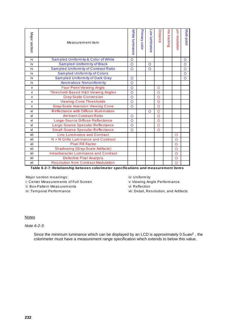
Major section
Meas urem ent item
White lum
inance
Prim
ary color
Low lum
inance
Distance
ms tracking
µm resolution
Four-Point Viewing AngleThreshold-Based H&V Viewing Angles
Gray-Scale Convers ionViewing-Cone Thres holds
Gray-Scale Invers ion Viewing ConeReflectance with Diffuse Illum ination
Am bient Contras t RatioLarge-Source Diffuse Reflectance
Large-Source Specular ReflectanceSm all-Source Specular Reflectance
Line Lum inance and Contras tN × N Grille Lum inance and Contras t
Pixel Fill FactorShadowing (Gray-Scale Artifacts )
Intracharacter Lum inance and Contras tDefective Pixel Analys is
Resolution from Contras t Modulation
Multi-point
iv Sam pled Uniform ity & Color of Whiteiv Sam pled Uniform ity of Blackiv Sam pled Uniform ity of Contras t Ratioiv Sam pled Uniform ity of Colorsiv Sam pled Uniform ity of Dark Grayiv Anom alous Nonuniform ityvvvvvviviviviviviiviiviiviiviiviiviiTable 6-2-7: Relationship between colorimeter specifications and measurement items
Major section m eanings :i: Center Measurem ents of Full Screenii: Box-Pattern Measurem entsiii: Tem poral Perform ance
iv: Uniform ityv: Viewing Angle Perform ancevi: Reflectionvii: Detail, Resolution, and Artifacts
Notes
Note 6-2-3:
Since the minimum luminance which can be displayed by an LCD is approximately 0.5 , the colorimeter must have a measurement range specification which extends to below this value.
232

6-2-4: Brief Definitions of Measurement Items
This section provides brief explanations of the measurement items specified in the VESA standard which can be measured with the CA-210. (For more detailed information, please refer to the VESA standard itself; see Note 6-2-4)
Luminance and Color of Full-Screen White
A full-screen white pattern is displayed and the luminance and chromaticity are measured at the center of the screen.
Luminance and Color of Full-Screen Black
A full-screen black pattern is displayed and the luminance and chromaticity are measured at the center of the screen.
Contrast Ratio of Full Screen
The full-screen white pattern measurement results (Lw) and full-screen black measurement results (Lb) are used to calculate the contrast ratio:
bw LL=Contrast
If the patterns which are measured are not full-screen patterns, or if the measurement is not taken normal to the screen surface, such conditions must be noted together with the contrast ratio.
Gamut and Colors of Full Screen
Full-screen RGB primary-color (or optionally CMY secondary-color) patterns are displayed in sequence, and the luminance and chromaticity of each pattern are measured at the center of the screen.
Gray Scale of Full Screen
8 (or optionally 16) full-screen gray test patterns from black to white are displayed in sequence, and the luminance of each pattern is measured at the center of the screen. The VESA gamma value can then be determined.
Color Scales of Full Screen
8 (or optionally 16) full-screen RGB primary-color (or optionally CMY secondary-color) patterns are displayed in sequence from highest luminance to black for each color, and the luminance of each pattern is measured at the center of the screen. The VESA gamma values for RGB primary colors (or optionally CMY secondary colors) can then be determined.
233

Full-Screen Gray-Scale Color Changes
8 (or optionally 16) full-screen gray test patterns from white to black are displayed in sequence, and the chromaticity of each pattern is measured at the center of the screen. The color change due to luminance changes is then be calculated. Color change is calculated in terms of distance in the u'v' color space u'v'.
Luminance Adjustment Range
For displays equipped with luminance adjustment functions, full-screen white patterns at maximum luminance (Lmax) and minimum luminance (Lmin) are displayed and the luminance of each pattern is measured in the center of the screen. The luminance adjustment range is then calculated as:
( ) [ ]% range adjustment Luminancemax
minmax
LLL −
=
Luminance and Contrast of Centered Box
A white box (with a diagonal 1/5 to 1/6 of the full screen diagonal) is displayed in the center of the screen on a black background, and the luminance at the center of the box (Lw1) and the luminance at 8 points in the black area surrounding the box are measured. The average of the black measurements (Lw2) is calculated, and the average contrast is then calculated as:
21Contrast ww LL=
Centered Box On-Off Luminance & Contrast
A white box (with a diagonal 1/5 to 1/6 of the full screen diagonal) is displayed in the center of the screen on a black background, and the luminance at the center of the box (Lw1) is measured. The white window is then replaced with black (so that the full screen is black) and the luminance at the center of the screen (Lw2) is measured. The contrast between the maximum luminance (Lw1) and the minimum luminance (Lw2) is then calculated as:
21Contrast ww LL=
Transverse Contrast of Centered Box
A white box (with a diagonal 1/5 to 1/6 of the full screen diagonal) is displayed in the center of the screen on a black background, the luminance at the center of the box (Lw1) is measured, and the luminance of points on the black screen area to the left and right of the box are measured and averaged (Lw2). The contrast is then calculated as:
21Contrast ww LL=
Gray Scale of Centered Box
A white box (with a diagonal 1/5 to 1/6 of the full screen diagonal) is displayed in the center of the screen on a black background, and the luminance of the box is changed in 8 (or optionally 16) steps from white to black in sequence. The luminance at the center of the box is measured for each step. The VESA gamma value can then be determined.
234

Color Gamut of Centered Box
A box (with a diagonal 1/5 to 1/6 of the full screen diagonal) is displayed in the center of the screen on a black background, and the RGB primary colors (or optionally CMY secondary colors) are displayed in the box in sequence, and the luminance and chromaticity of each pattern are measured at the center of the box.
Color Scales of Centered Box
A box (with a diagonal 1/5 to 1/6 of the full screen diagonal) is displayed in the center of the screen on a black background, and the RGB primary colors (or optionally CMY secondary colors) are displayed in the box as the luminance of the color is changed in 8 (or optionally 16) steps in sequence, and the luminance and chromaticity of each step are measured at the center of the box. The VESA gamma values for RGB primary colors (or optionally CMY secondary colors) can then be determined.
Halation
A black box is displayed in the center of the screen on a white background, and the size of the box is changed in steps. The luminance at the center of the box is measured for each step and the relation between the box size and luminance is determined.
Halation is defined as:
w
b
LLL −
= maxHalation
where Lmax is the maximum luminance measured in this sequence, Lb is the luminance for a full-screen black measured in this sequence, and Lw is the luminance for a full-screen white measured in this sequence.
Luminance Loading
A white box is displayed in the center of the screen on a black background, and the size of the box is changed in steps. The luminance at the center of the box is measured for each step and the relation between the box size and luminance is determined.
Loading is defined as:
w
wext
LLL −
=Loading
where Lext is the maximum luminance measured in this sequence and Lw is the luminance for a full-screen white measured in this sequence.
Checkerboard Luminance and Contrast
A checkerboard pattern (such as that shown in Figure 6-2-1) is displayed on the screen, the luminance of white and black areas near the center of the screen are measured, and the contrast is determined from the measured values. (Contrast equation is the same as for Luminance and Contrast of Centered Box.)
235

Residual Image
The residual image after displaying a checkerboard image is evaluated according to the following procedure:
• Measurement points for this procedure are the center of a white block B (like Area B in Figure 1) and a black block A (like Area A in Figure 1) of a checkerboard pattern.
1 A full-screen white pattern is displayed and the luminance of points A and B (LA and LB respectively) are measured.
2 A checkerboard pattern like that shown in Figure 1 is then displayed for a specified period of time.
3 The display is then returned to a full-screen white pattern, and the luminance of points A and B (KA and KB respectively) are measured.
Residual image factor is defined as:
BA
AB
KKLL −= 1Factor Image Residual
Warm-Up Time Measurement
The luminance of the LCD is measured periodically from the time the LCD is switched on and the time required for the luminance variation over time to reach 5% or less (relative to the stable luminance level) is measured.
It is important that the temperature of the LCD be the same as the ambient temperature prior to switching on the LCD.
Dominant Flicker Component
The luminance variation when flicker occurs is measured, and after the frequency components have been determined, the flicker value is calculated based on the DC component and the maximum frequency component. The result is luminance variation characteristics that include the influence of the frequency response characteristics of the human eye.
(See section 1-7-2-1: Flicker Measurement.)
Flicker Modulation Amplitude
The luminance variation when flicker occurs is measured, and the ratio between the DC component and the modulation amplitude is determined. The result is luminance variation characteristics that include the influence of the frequency response characteristics of the human eye.
(See section 1-7-2-1: Flicker Measurement.)
Sampled Uniformity & Color of White
A full-screen white pattern is displayed. The luminance and chromaticity are measured at 5 (or 9) points on the screen, and the luminance uniformity and chromaticity uniformity are determined. Luminance uniformity is defined as:
236

[ ]%uniformity Luminancemax
minmax
LLL −
=
where Lmax is the maximum luminance measured and Lmin is the minimum luminance measured.
Chromaticity uniformity is defined as the maximum distance between any two measured points in the u'v' color space.
Sampled Uniformity of Black
A full-screen black pattern is displayed. The luminance is measured at 5 (or 9) points on the screen, and the luminance uniformity is determined. Luminance uniformity is defined as:
[ ]%uniformity Luminancemax
minmax
LLL −
=
where Lmax is the maximum luminance measured and Lmin is the minimum luminance measured.
Sampled Uniformity of Contrast Ratio
A full-screen white pattern is displayed, and the luminance is measured at 5 (or 9) points. The screen is then switched to a full-screen black pattern, and the same points are measured again. The contrast for each point i is then calculated as:
[ ]%Contrast bwi LLC =
where Lw is the measured white-screen luminance and Lb is the measured black-screen luminance at that point.
The contrast non-uniformity for the screen is then calculated from the maximum and minimum contrast values (Cmax and Cmin respectively) of all the measured points, using the equation:
[ ]%ityNonuniformmax
minmax
CCC −
=
Sampled Uniformity of Colors
A full-screen solid-color pattern is displayed. The luminance and chromaticity are measured at 5 (or 9) points on the screen, and the luminance uniformity and chromaticity uniformity are determined. Luminance uniformity and chromaticity uniformity are defined as in Sampled Uniformity & Color of White.
Sampled Uniformity of Dark Gray
A full-screen dark-gray pattern is displayed. The luminance and chromaticity are measured at 5 (or 9) points on the screen, and the luminance uniformity and chromaticity uniformity are determined. Luminance uniformity and chromaticity uniformity are defined as in Sampled Uniformity & Color of White.
Anomalous Nonuniformity
A full-screen white pattern is displayed, and the screen areas with the maximum and minimum luminance are determined. The luminance is measured at those points, and the luminance uniformity is determined as defined in Sampled Uniformity & Color of White.
237

Notes
Note 6-2-4:
The VESA standards can be purchased from the VESA home page at:
http://www.vesa.org
238

6-3: sRGB
6-3: What is sRGB?
In the past, the fact that there were differences between the images produced by image output devices (displays and printers) and the colors of the actual objects.
Two methods for solving this problem have been proposed:
1 Perform compensation using color profiles for each image input and output device.
2 Provide a common color space (standard color space) for all image input and output devices to use.
For method 1, the method defined by the ICC (International Color Consortium) is well known. But this method has the problems of requiring the input/output profile for the object (whose color can be reproduced with high fidelity) to be embedded in the subject image, and the processing to determine the color places a heavy load on the device.
For method 2, since the image input or output device processes image data based on the standard color space, the load on the device is not so great, and the true color of the object can be reproduced with high fidelity.
sRGB is one standard color space based on method 2, and was standardized in IEC-61966-2-1. Currently, for typical image input and output devices such as digital cameras, LCDs, CRTs, printers, etc., products which conform to sRGB are being sold. In addition, it is also used as the default color space for many Web languages and operating systems.
R G Bx 0.6400 0.3000 0.1500y 0.3300 0.6000 0.0600
Table 6-3-1: Corners of sRGB color space
Lum inance level 80cd/m 2
White point D65 (x=0.3127, y=0.3291)
Gam m a characteris tics γ=2.2
Table 6-3-2: sRGB reference conditions
The standard color space defined by sRGB is shown in Figure 6-3-1 and Table 6-3-1. In addition, the reference conditions which should be criteria for displays are shown in Table 6-3-2. Table 6-3-1 also shows the NTSC color space defined for CRTs.
You can see that the sRGB color space is smaller than the NTSC color space. Since the display color space for sRGB is relatively small, some problems remain, such as that some colors in silver-halide photographs cannot be reproduced. Discussions on the establishment of standards to solve these problems are underway.
239

References
Hiroaki Sugiura, Imaging Information Media Society Magazine, Vol. 56 No. 8, pp. 1247-1248 (2002)
240

241

Index A About Color-Measuring Instruments...................................................................................... 15 Absolute-Value Error ............................................................................................................. 19 Accuracy .......................................................................................................................... 89, 91 Advantages of Successive A/D method ................................................................................ 52 Analyzer Mode Calculations ........................................................................................................................... 33 Overview................................................................................................................................ 30 Principle ................................................................................................................................. 31
C CA-100/CA-100Plus Measurement Error for CRT/PDP Measurements Measurement of White High Luminance (CRT)........................................................................................................ 149 Measurement of White (PDP).............................................................................................. 151 Measurmenet of White Low Luminance (CRT)......................................................................................................... 150 Repeatability Comparison ................................................................................................... 152 CA-210 Application Example Gamma Adjustment Gamma Adjustment Process............................................................................................... 282 GUI ...................................................................................................................................... 285 Introduction .......................................................................................................................... 280 System Block Diagram ........................................................................................................ 281 White Balance Adjustment Gamma Adjustment Time.................................................................................................... 284 GUI ...................................................................................................................................... 277 Introduction .......................................................................................................................... 272 System Block Diagram ........................................................................................................ 274 White Balance Adjustment Software Functions .................................................................. 275 White Balance Adjustment Time ......................................................................................... 276 CA-210 System Accuracy.................................................................................................... 110 Calibration Matrix Calibration....................................................................................................... 35, 36, 37 Of tristimulus colorimeters ..................................................................................................... 20 User calibration................................................................................................................ 23, 24 CA-SDK C++ Adding Code for the UI Objects........................................................................................... 174 CA-SDK Object Creation ..................................................................................................... 176 Const.h File.......................................................................................................................... 191 Creating the Application Project .......................................................................................... 172 Creating the Sink Object...................................................................................................... 183 Creating the UI (User Interface) .......................................................................................... 173 Error Handling...................................................................................................................... 190 Sink Object Creation/Connection and Event Handling........................................................ 187 Using the CA-SDK Objects.................................................................................................. 180 C++ (Details) Adding Code for the UI Objects........................................................................................... 202 CA-SDK Object Creation ..................................................................................................... 206 Const.h File.......................................................................................................................... 213 Creating the Application Project .......................................................................................... 195 Creating the SDK Application .............................................................................................. 194 Creating the Sink Object...................................................................................................... 209 Creating the UI (User Interface) .......................................................................................... 200 Sink Object Creation/Connection and Event Handling........................................................ 212 Using the CA-SDK Objects.................................................................................................. 208
242
CA-SDK Sample Software Control Methods ....................................................................... 216 COM Automation........................................................................................................................... 165 Introduction .......................................................................................................................... 155 COM Interface ..................................................................................................................... 158 COM Interface Programming............................................................................................... 161 Control Methods CaControl Using in VB.......................................................................................................................... 221 Using in VC++ (MFC) .......................................................................................................... 224 CaControl (for Performing Settings on CA-Series Instruments).......................................... 218 CaControl Properties/Methods ............................................................................................ 219 xyControl Using in VB.......................................................................................................................... 235 Using in VC++ (MFC) .......................................................................................................... 237 xyControl (for Displaying Data in xy Color Space) .............................................................. 231 xyControl Properties/Methods ............................................................................................. 232 Creating a VC++ application using the CA-SDK ................................................................. 170 Interface............................................................................................................................... 157 Regarding COM................................................................................................................... 167 VB Sample Software Calibration.................................................................................................................... 247, 248 Color/Flicker Measurement ................................................................................................. 241 Contrast Measurement ........................................................................................................ 246 Gamma Measurement......................................................................................................... 245 Introduction .......................................................................................................................... 240 Visual Basic .NET Creating an Application in Visual Basic .NET usign the CA-SDK ....................................... 253 Creating the VB.NET Project............................................................................................... 254 Creation of Application GUI/Code ....................................................................................... 261 Setting references to CA_SDK............................................................................................ 256 Chromaticity..................................................................................................................... 12, 13 CIE......................................................................................................................................... 12 Circuit Features ..................................................................................................................... 50 Color Measuring .............................................................................................................................. 13 Color matching functions ....................................................................................................... 13 Color systems ........................................................................................................................ 12 Concept of Matrix Calibration ................................................................................................ 36 Contrast Method .............................................................................................................. 62, 63 Data Processing .................................................................................................................... 63 Copyrights/Trademarks ........................................................................................................... 9
E ED-2522 CA-210 and ED-2522 Standards Brief Definitions of Measurement Items............................................................................... 293 Introduction .......................................................................................................................... 289 Measurement Items............................................................................................................. 290 Measurement Items and CA-210......................................................................................... 291
F Flicker Accuracy Standards and Repeatability ............................................................................... 103 Basic Concept of Flicker Measurement Accuracy/Repeatability......................................... 106 Contrast Method .............................................................................................................. 62, 63 Definition of Accuracy.......................................................................................................... 105 Definition of Repeatability.................................................................................................... 112 How Flicker Occurs................................................................................................................ 56 Images/Drive Systems Likely to Cause Flicker ..................................................................... 57
243
JEITA Method ........................................................................................................................ 68 Measurement examples ........................................................................................................ 58
I Inputting RGB Emission Characteristics ............................................................................... 31 Inter-Instrument Error Of tristimulus colorimeters ..................................................................................................... 25 Introduction .............................................................................................................................. 7
J JEITA Method Data processing..................................................................................................................... 72 Data processing by CA-210................................................................................................... 74 Differences from Contrast Method......................................................................................... 73 Differences from VESA method............................................................................................. 78 Equation................................................................................................................................. 76 Equation (Additional Information) .......................................................................................... 77 Equation Used by CA-210 ..................................................................................................... 75
L Low-Luminance Measurement .............................................................................................. 46 Luminance Range.................................................................................................................. 90 Certified Accuracy.................................................................................................................. 90 Luminance/Chromaticity Accuracy Standards....................................................................... 87 Luminance/Chromaticity Variation......................................................................................... 48
M Main Body Section............................................................................................................... 107 Matrix Calibration Concept ................................................................................................................................. 36 RGB Calibration..................................................................................................................... 39 WRGB Calibration ................................................................................................................. 41 Matrix Calibration Overview................................................................................................... 35 Measurement Accuracy................................................................................................. 98, 114 Measurement Results - CA-210 LCD Flicker Measuring Probe/CS-1000 Measurements of Primary Colors ........................................................................................ 133 Measurements of White....................................................................................................... 132 Measurement Results - CRT Measurements with CA-100/CA-100Plus Measurements of Primary Colors ........................................................................................ 145 Measurements of White....................................................................................................... 144 Measurement Results - LCD Measurements with CA-210/CA-110/CS-1000 Measurement of Intermediate Colors .................................................................................. 124 Measurement of Primary Colors.......................................................................................... 122 Measurement of White High Luminance................................................................................................................... 117 Low Luminance.................................................................................................................... 120 Measurement Results - Flicker Measurements Contrast Method .................................................................................................................. 135 JEITA Method ...................................................................................................................... 137 Measurement Results- Gamma Characteristics Measurements......................................... 127 Measurement Speed ........................................................................................................... 141
N Narrow Viewing Angle/Uniform Viewing Angle...................................................................... 47
O Optical System Features ....................................................................................................... 44
244

P PDP Relation to Chromatic Luminance Meter ............................................................................... 83 What is a PDP? ..................................................................................................................... 80 Probe Section ...................................................................................................................... 109
R Repeatability .............................................................................................................. 94, 95, 96 Definition of............................................................................................................................ 94 RGB Calibration..................................................................................................................... 39 RGB Emission Characteristics - Inputting ............................................................................. 31
S Spectroradiometer ................................................................................................................. 17 Spectroradiometers ............................................................................................. 15, 26, 27, 28 vs. tristimulus colorimeters .................................................................................................... 26 sRGB ................................................................................................................................... 310 Standards CA-210 and ED-2522 Standards Brief Definitions of Measurement Items............................................................................... 293 Introduction .......................................................................................................................... 289 Measurement Items............................................................................................................. 290 Measurement Items and CA-210......................................................................................... 291 CA-210 and VESA Standards Brief Definitions of Measurement Items............................................................................... 303 Introduction .......................................................................................................................... 296 Measurement Conditions and CA-210 ................................................................................ 297 Measurement Items and CA-210......................................................................................... 300 sRGB ................................................................................................................................... 310 Successive A/D method ........................................................................................................ 52 Advantages............................................................................................................................ 52
T Traceability .......................................................................................................................... 100 Tristimulus Colorimeters.............................................................. 15, 16, 19, 21, 25, 26, 27, 28 Absolute-value error for ......................................................................................................... 19 Calibration........................................................................................................................ 21, 22 Inter-instrument error ............................................................................................................. 25 User calibration of.................................................................................................................. 23 vs. Spectroradiometers.......................................................................................................... 26
U User-calibration...................................................................................................................... 24 u'v'.......................................................................................................................................... 13
V VESA Standard Flicker Method............................................................................................. 65 VESA Standards CA-210 and VESA Standards Brief Definitions of Measurement Items............................................................................... 303 Introduction .......................................................................................................................... 296 Measurement Conditions and CA-210 ................................................................................ 297 Measurement Items and CA-210......................................................................................... 300
W WRGB Calibration ................................................................................................................. 41
245

X xyLv ....................................................................................................................................... 16 XYZ.................................................................................................................................. 13, 16
246