Intraday Evidence of the Informational

Efficiency of the Yen/Dollar Exchange Rate

Kentaro Iwatsubo Yoshihiro Kitamura

April 2008 Discussion Paper No.0801

GRADUATE SCHOOL OF ECONOMICS

KOBE UNIVERSITY

ROKKO, KOBE, JAPAN

Intraday Evidence of the Informational Efficiency of the

Yen/Dollar Exchange Rate☆

Kentaro Iwatsuboa and Yoshihiro Kitamurab,*

a Graduate School of Economics, Kobe University, Hyogo, Japan

b Faculty of Economics, University of Toyama, Toyama, Japan

Abstract The informational efficiency of the yen/dollar exchange rate is investigated in five market segments within each business day from 1987 to 2007. Among the results, we first find that the daily exchange rate has a cointegrating relationship with the cumula-tive price change of the segment for which the London and New York markets are both open, but not with that of any other segments. Second, the cumulative price change of the London/N.Y. segment is the most persistent among the five market segments in the medium- and long-run. These results suggest that the greatest concentration of informed traders is in the London/N.Y. segment where intraday transactions are the highest. This is consistent with the theoretical prediction by Admati and Pfleiderer (1988) that prices are more informative when trading volume is heavier. JEL classification: F31 Keywords: Informational efficiency; Market segments; Yen/dollar exchange rate

*Corresponding author. 3190 Gofuku, Toyama 930-8555 Japan. tel.: +81-76-445-6475; e-mail address: kitamu@eco.u-toyama.ac.jp (Y. Kitamura).

☆ We thank the participants of the Institute of Statistical Research Conference in Bar-celona for useful comments. This work is financially supported by Grant-in-Aid for Young Scientists (B18730211, K. Iwatsubo; B19730216, Y. Kitamura) and Yamada Academic Research Promotion Fund.

1. Introduction Foreign exchange markets do not sleep. Traders can exchange currencies 24 hours a day

in any market around the world if trading counterparties are available. Nevertheless, in

reality reasonably well-defined opening and closing times do exist and the activity of

each market has a typical intraday seasonality. Several recent studies exploit the Elec-

tronic Broking Services (EBS)1 data to document intraday volume patterns in the for-

eign exchange market (Chaboud et al. (2004, 2007), Ito and Hashimoto (2006), and Cai

et al. (2007))2. Ito and Hashimoto (2006) find that there is a U-shape pattern of volume

– namely, heavy trading in the beginning and at the end of the trading day and relatively

light trading in the middle of the day – in the Tokyo and London markets for the

yen/dollar and euro/dollar rates, but not in the N.Y. market of those currencies. A more

notable confirmed feature is that the overlapping business hours encourage in-

ter-regional transactions and an overall surge in activities. For the yen/dollar transac-

tions, for example, trading volume is the highest when the London and New York busi-

ness hours overlap and the second highest when the Tokyo and London markets are

both open (Figure 1). Taken together, this evidence suggests that the U-shape pattern of

intraday volume results from the concentration of transactions during overlapping busi-

ness hours.

******** Figure 1 around here *******

The objective of this paper is to investigate the empirical link between intraday

trading volume and informational efficiency. There has been a great deal of empirical

work on the volume-volatility relationship (e.g. Tauchen and Pitts (1983)), but there are

few studies on the relationship between volume and informational efficiency. Our re-

sults help clarify why trading volume is high during the overlapping business hours of

foreign exchange markets.

There are two polar views regarding the relationship between volume and in-

formational efficiency: the asymmetric information view and the inventory control view.

1 In the last few years, the brokers markets have been revolutionalized by the introduc-tion of two electronic broking systems (Reuters D2002-2 and Electronic Broking Ser-vices [EBS]) which have effectively taken over from voice brokers. 2 Chaboud et al. (2004, 2007) and Cai et al. (2007) find sharp spikes in volume at the times of scheduled macroeconomic data releases, spot foreign exchange fixings, and the standard expiration times of foreign exchange options.

1

The asymmetric information view argues that trades are more informative when trading

volume is high, while the inventory control view holds that trades are less informative

when trading volume is high. Theory admits both possibilities, depending on the posited

information structure.

To understand the asymmetric information view, consider the model of Admati

and Pfleiderer (1988). In order to minimize their losses to informed traders, discretion-

ary liquidity traders prefer to trade when the market is thick – that is, when their trading

has little effect on prices. With more liquidity trading in a given period, more informed

traders tend to trade with liquidity traders. This makes it even more attractive for liquid-

ity traders to trade in that period because competition among the informed traders re-

duces their total profit, which benefits the liquidity traders. Admati and Pfleiderer

(1988) argue that these strong incentives for the concentration of trading create the

U-shape pattern of intraday volume. An increase in the number of informed traders con-

tributes to the informativeness of prices because they cause prices to adjust faster to in-

formation. In this situation, trading volume and the informational efficiency of prices

are positively related.

On the other hand, the representative model of the inventory control view is

developed by Lyons (1997). On the inventory control side, the key mechanism is hot

potato trading – passing unwanted positions from dealer to dealer following an initial

customer order. To clarify the argument, consider the following example. Suppose that

there are ten dealers, all of whom are risk averse and currently hold zero positions. A

customer sale of $10 million worth of Japanese yen is accommodated by one of the

dealers. Not wanting to carry the open position, the dealer calculates his share of this

inventory imbalance – or one-tenth of $10 million – calls another dealer, and unloads $9

million worth of Japanese yen. The dealer receiving his trade then calculates his share

of this inventory imbalance – or one tenth of $9 million – calls another dealer, and

unloads $8.1 million worth of Japanese yen. The hot potato process continues. In the

limit, the total interdealer volume guaranteed from the $10 million customer trade is $9

million / (1-0.9) = $90 million. This simple example illustrates that the repeated passage

of idiosyncratic inventory imbalances among dealers following an innovation in cus-

tomer order flow can better explain the high transaction volume in foreign exchange

markets.

2

Hot potato trading reduces the informativeness of prices. Information aggrega-

tion by dealers occurs through signal extraction applied to order flow. The greater the

noise relative to the signal, the less effective signal extraction is. Passing the hot potato

trades increase the noise in order flow and dilute informational content. Hence, trading

volume and the informational efficiency of prices are negatively linked.

In this paper, we provide evidence that discriminates between the two views.

Our paper shares the same motivations as the studies by Lyons (1995, 1996), in which

real-time transaction data are used to document that trades occurring when intertransac-

tion times are short are significantly less informative, supporting the inventory control

view. In his work, intertransaction times are used as a proxy for trading volume. As

Lyons (1995, 1996) admits, however, the assumption that intertransaction times are ex-

ogenous may be problematic because earlier work (e.g., Hausman, Lo and MacKinlay,

1992) has tested for and rejected the exogeneity of the length of time between transac-

tions at a conventional significance level. The short sample period covering only five

trading days of the week is another caveat (Mello, 1996).

The current paper takes a different approach to the analysis of the vol-

ume-information relationship. Taking the intraday volume pattern as exogenous, we

examine the information efficiency of the intraday yen/dollar rate. Specifically, we split

the foreign exchange market into five market segments (Tokyo, London-only, Lon-

don/N.Y. overlap, N.Y.-only, and Pacific) and compare price informativeness among

the segments.

A key feature of our analysis is the use of long-term data for a period of 20

years spanning from 1987 to 2007. This enables us to provide robust empirical evidence

on informational efficiency and the volume-information relationship. Although Ito and

Hashimoto (2006) reveal that intraday patterns of volume have been quite stable in re-

cent years, in spite of the technological advances and the introduction of the electronic

broking system, they may have changed gradually over the last two decades. It is a

well-known stylized fact, however, that transaction volume is the highest in the segment

where the London and N.Y. markets are both open (see Guillaume et al., 1995). Based

on this fact, we explore the price informativeness between the market in overlapping

business hours (London/N.Y.) and the rest of the market segments and consider the

volume-information relationship. We believe that the endogeneity problem is partially

3

solved, without resorting to the use of high-frequency exchange rate and order flow data,

by exploiting the stylized fact that trading volume has been higher in the London/N.Y.

segment than in any other segment.

Another notable feature of this paper is the introduction of a new concept for

intraday exchange rate analysis: the “cumulative price change” of market segments. The

daily yen/dollar exchange rate change from t to t+1 ( ), measured at

the Tokyo opening, can be decomposed into the price changes of the five market seg-

ments:

TYt

TYtt PPP −=∆ ++ 11

,/1

PAt

NYt

NLt

LNt

TYtt PPPPPP ∆+∆+∆+∆+∆=∆ +

TYtP∆

OPTYt

CLTYt

TYt PPP ,, −= LN

tP∆CLTY

tOPNY

tLN

t PPP ,, −= NLtP /∆

OPNYt

CLLNt

NLt PPP ,,/ −=∆

NYtP∆

CLLNt

CLNYt

NYt PPP ,, −= PA

tP∆, ,

1

(1)

where is the price change in the Tokyo segment (TY) from its opening to closing

(∆ ), is that in the London segment (LN) from the Tokyo

closing to the N.Y. opening (∆ ), is that in the London/N.Y.

overlap (L/N) from the N.Y. opening to the London closing ( ),

is that in the N.Y. segment (NY) from the London closing to the N.Y. closing

(∆ ), and is that in the Pacific segment (PA) from the N.Y.

closing to the Tokyo opening ( PA TY OP NY CLt t tP P P+∆ = −

1

). The superscripts OP and CL of

the price P refer to the opening and closing rates, respectively. The data is described in

Section 2.

Summing both sides of Equation (1) from =t s

.111

/

1111 ∑∑∑∑∑∑

======+ ∆+∆+∆+∆+∆=∆

s

t

PAt

s

t

NYt

s

t

NLt

s

t

LNt

TYt

s

t

s

tt PPPPPP

1

to , we obtain the following

equation:

(2)

On the left-hand side of Equation (2), the total change in the daily exchange

rate is equal to Ps+1–P1, that is, the daily exchange rate at += st

1=t s

./11

PAs

NYs

NLs

LNs

TYss CPCCPCCPCCPCCPCPP ++++=−+

minus its initial

value P1 (constant). On the other hand, the right-hand side equals the sum of the cumu-

lative price changes of the five market segments. The cumulative price change (CPC,

hereafter) represents the aggregated price changes of each segment from to .

Equation (3) is a simple representation of Equation (2).

(3)

One of the advantages of exploiting CPCs is their nonstationarity, which allows

us to measure the size of the random walk in each CPC and hence analyze

(weak-form) informational efficiency. On the contrary, a caveat of using CPCs to

4

compare price informativeness is that CPCs are assumed to be independent from each

other. If exchange rate changes in one market segment have interregional impacts, this

assumption may be problematic. In the literature of exchange rate volatility clustering,

Engle et al. (1990) find support for the meteor shower effect (interregional volatility

spillover), while Baillie and Bollerslev (1990) and Melvin and Melvin (2003) report

evidence for the heat wave effect (own-region volatility persistence). Cai et al. (2007)

revisit this issue using the EBS data and confirm that both effects are present. However,

their results based on exchange rate returns (not volatility) suggest that informational

linkages across trading regions are so limited that their economic significance is very

small. Therefore, we do not think that the assumption of independency misleads our

conclusions. To check robustness, we take the interdependency of CPCs into account

in the analysis of section 3-3.

Fama (1970), summarizing the idea of informational efficiency in his classic

survey, writes: “A market in which prices always ‘fully reflect’ available information is

called ‘efficient’.” In an informationally efficient market, price changes must be un-

forecastable if they fully incorporate the expectations and information of all market par-

ticipants. In practice, since it is almost impossible to take traders’ information and ex-

pectations into consideration, much research on the market efficiency hypothesis tests

the forecastablility of prices based only on past price changes. Among various versions

of the weak-form informational efficiency, many researchers investigate the random

walk hypothesis. We test this hypothesis with variance ratio tests which exploit the im-

portant property of the random walk process that the variance of random walk incre-

ments must be a linear function of the time interval.

The second hypothesis is that, in an informationally efficient market, the CPCs

contribute significantly to the long-run trend of exchange rates. If the CPCs are infor-

mational efficient, they must have a stable relationship with the daily exchange rate in

the long run. We explore whether there is any cointegration relationship between the

daily exchange rate Ps+1 and the CPC of each segment with careful consideration of

structural breaks.

Among the results, we first find that the daily exchange rate has a cointegration

relationship with the CPC of the overlapping business hours in the London/N.Y. seg-

ment, but not with any other segments. Second, the CPC of the London/N.Y. segment is

5

the most persistent among all five segments. The evidence indicates that the price

change of the London/N.Y. segment is the most informationally efficient. From a

long-term perspective, this evidence supports the asymmetric information view that

trades are more informative when trading volume is high.

The organization of this paper is as follows. Section 2 briefly explains the data

and basic statistics. Section 3 shows several empirical results and Section 4 concludes.

2. Data In order to examine the informational efficiency of the intraday yen/dollar rate, we

identify five separate periods for classifying regional hours: Tokyo, London-only, Lon-

don/N.Y. overlap, N.Y.-only, and Pacific. We obtain the Tokyo opening and closing

rates, the London closing rate, and the N.Y. opening and closing rates from the Nikkei

Needs Financial Quest system.3 The sample period runs from September 14, 1987 to

May 31, 2007, based on data availability. Missing data, due to national holidays, are

replaced with the closest data from the previous segment. The timing of the market seg-

ments is as follows: the Tokyo opening and closing rates are recorded at 9:00 a.m. and

17:00 p.m. in local time, respectively. Since the London opening is unavailable in our

long-run data set but is very close to the Tokyo closing4, we adopt the Tokyo closing as

a proxy for the London opening. The London market closes at 16:00 p.m.5, and the N.Y.

market opens at 8:30 a.m. and closes at 17:00 p.m. in local time.

*****Table 1 around here*****

Table 1 displays the time schedule for the five market segments. We take into

account differences in the duration of each segment due to daylight saving time. Foreign

exchange trading starts in the Tokyo market, and the London market opens just after the 3 The Nikkei Needs database collects the mid-points of TTS (Telegraphic Transfer Selling rate) and TTB (Telegraphic Transfer Buying rate). 4 Melvin and Melvin (2003) and Cai et al. (2007) identify the period in which Tokyo and London business hours overlap, while we include the overlap in the Tokyo segment. By their definition of the London opening time, however, the length of the To-kyo/London overlap is short, 1.5h in normal time (2.5h in DST) 5 Since the WM/Reuters spot foreign exchange fixing occurs at 16:00 p.m. in London, the 16:00 p.m. FX rate is commonly used. We are aware that 16:00 p.m. is a little earlier than the actual closing time of the London market. This may lead to a shorter Lon-don/N.Y. segment than the actual. Hence, our conservative definition of the segment does not give misleading results.

6

Tokyo market closes. Since the N.Y. market opens before the London closes, active

trading takes place when both markets are open for several hours. The N.Y. market

closes several hours after the London market. By our definition, the Pacific market (e.g.,

Sydney) is very limited, starting from the N.Y. closing to the Tokyo opening on the next

day. Although this short period is included in the Asia segment in the analysis of Cai et

al. (2007), as shown in Figure 1, the yen/dollar trading in this market segment is the

least active in a day.

*****Table 2 around here*****

Table 2 presents the summary statistics on price changes for the five market

segments. The per hour variance of price changes for each segment are shown, and is

defined as the variance adjusted for the number of trading hours in each market segment.

To correct for differences in segment duration, we divide the price change (∆Pit) by the

square root of business hours in segment i on date t and calculate its variance. The fifth

column of Table 2 reports the variance ratio of the returns of London/N.Y. to those of

each segment. Simple variance ratio tests reveal that the London/N.Y. segment is far

more volatile than any other segment. This is consistent with Ito and Roley’s (1987)

argument that the high volatility on late London and early N.Y. business hours may re-

flect a great deal of news coming from the European and N.Y. markets.

3. Empirical Analysis 3.1. Cointegration tests

Figures 2-1 through 2-5 show the CPC for each segment and the daily exchange rate

throughout the sample period. We adopt the Tokyo opening rate at t+1 as the daily

yen/dollar rate. In Figure 2-3, we observe a long-run stable relationship between the

daily exchange rate and the London/N.Y. CPC. It is also noteworthy that the Tokyo

CPC shows a steadily depreciation in the dollar since 2000, while the N.Y. CPC shows

a constant appreciation of the dollar during the same period. This sharp contrast is puz-

zling, but we limit ourselves to pointing out this phenomenon.

*****Figures 2 around here*****

We next conduct empirical tests on the stability of the relationship between the

daily yen/dollar rate and the CPC. The stable relationship suggests that exchange rate

pricing in the market segments greatly contributes to the determination of long-run ex-

7

change movements.

To test these hypotheses, we regress the daily yen/dollar rate (the Tokyo open-

ing rate at t+1), onto each CPC at t and perform residual-based cointegration tests. Be-

fore the cointegration analyses, we confirm the nonstationarity of each variable using

ADF unit root tests. The results, presented in Table 3, indicate that all variables have a

unit root in levels but not in first differentials. This indicates that they are all integrated

of order one (I(1)).6

*****Table 3 around here*****

*****Table 4 around here*****

The results of the cointegration test (ADF-type test) in Table 4 suggest that a

cointegration relationship is found only between the daily yen/dollar rate and the Lon-

don/N.Y. CPC. This result is consistent with the evidence that appears in Fig 2., but

should be treated carefully because ADF-type tests have a low power of rejection for the

unit root hypothesis in stationary variables with a structural break. An alternative test is

to consider the existence of structural breaks. Gregory and Hansen (1996a, b) developed

a cointegration test which allows for the possibility of a regime shift. The virtue of their

test is that the structural break point is endogenously determined rather than being as-

sumed to be predetermined. Following Gregory and Hansen (1996a), we consider the

following three types of regression models:

(1) “Level shift” model (Model C)

,11 ++ +++= tittt CPCDP νβδα α

,11 ++ ++++= titt

ittt CPCDCPCDP νδβδα βα

,11 ++ ++++++= ttitt

ittt TrendDTrendCPCDCPCDP νδγδβδα γβα

(4)

(2) “Regime shift” model (Model C/S) (5)

(3) “Regime and trend shift” model (Model C/S/T) (6)

where Dt is a dummy variable with a value of unity after the break point period and zero

6 The ADF test statistic is calculated with the assumption of whiteness of residuals

(Hamilton (1994)). Although the Lag 1 ADF test statistic for the level of the daily rate is

statistically significant at 10%, this result is dubious since the Portmanteau statistic

[Q(10)] for its residuals rejects no serial correlations at the 1% significance level

(Q[10]=31.015).

8

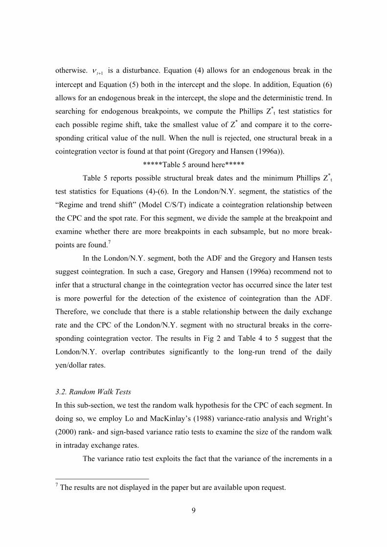
otherwise. 1+tν is a disturbance. Equation (4) allows for an endogenous break in the

intercept and Equation (5) both in the intercept and the slope. In addition, Equation (6)

allows for an endogenous break in the intercept, the slope and the deterministic trend. In

searching for endogenous breakpoints, we compute the Phillips Z*t test statistics for

each possible regime shift, take the smallest value of Z* and compare it to the corre-

sponding critical value of the null. When the null is rejected, one structural break in a

cointegration vector is found at that point (Gregory and Hansen (1996a)).

*****Table 5 around here*****

Table 5 reports possible structural break dates and the minimum Phillips Z*t

test statistics for Equations (4)-(6). In the London/N.Y. segment, the statistics of the

“Regime and trend shift” (Model C/S/T) indicate a cointegration relationship between

the CPC and the spot rate. For this segment, we divide the sample at the breakpoint and

examine whether there are more breakpoints in each subsample, but no more break-

points are found.7

In the London/N.Y. segment, both the ADF and the Gregory and Hansen tests

suggest cointegration. In such a case, Gregory and Hansen (1996a) recommend not to

infer that a structural change in the cointegration vector has occurred since the later test

is more powerful for the detection of the existence of cointegration than the ADF.

Therefore, we conclude that there is a stable relationship between the daily exchange

rate and the CPC of the London/N.Y. segment with no structural breaks in the corre-

sponding cointegration vector. The results in Fig 2 and Table 4 to 5 suggest that the

London/N.Y. overlap contributes significantly to the long-run trend of the daily

yen/dollar rates.

3.2. Random Walk Tests

In this sub-section, we test the random walk hypothesis for the CPC of each segment. In

doing so, we employ Lo and MacKinlay’s (1988) variance-ratio analysis and Wright’s

(2000) rank- and sign-based variance ratio tests to examine the size of the random walk

in intraday exchange rates.

The variance ratio test exploits the fact that the variance of the increments in a

7 The results are not displayed in the paper but are available upon request.

9

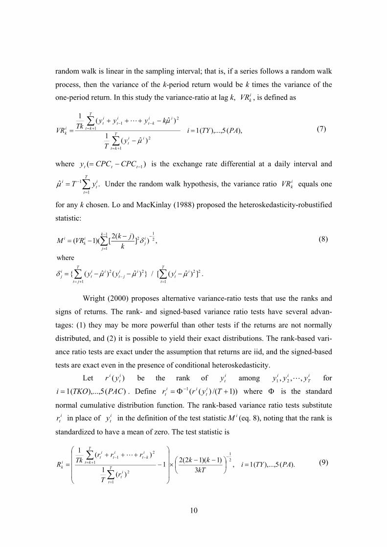
random walk is linear in the sampling interval; that is, if a series follows a random walk

process, then the variance of the k-period return would be k times the variance of the

one-period return. In this study the variance-ratio at lag k, , is defined as ikVR

),(5),...,(1)ˆ(1

)ˆ(1

1

2

1

21

PATYiy

T

kyyyTkVR T

kt

iit

T

kt

iikt

it

it

ik =

−

−+++=

∑

∑

+=

+=−−

µ

µ

)( 1−

(7)

where −= ttt CPCCPCy

1

1

ˆ . T

i it

tT yµ −

=

= ∑ ikVR

is the exchange rate differential at a daily interval and

Under the random walk hypothesis, the variance ratio equals one

for any k chosen. Lo and MacKinlay (1988) proposed the heteroskedasticity-robustified

statistic:

112 2

1

2 2 2 2

1 1

2( )( 1)( [ ] ) ,

where

ˆ ˆ ˆ{ ( ) ( ) } / [ ( ) ] .

ki i i

k jj

T Ti i i i i i ij t t j t

t j t

k jM VRk

y y y

δ

δ µ µ µ

− −

=

−= + =

−= −

= − − −

∑

∑ ∑

)it

i ity i

Tii yyy ,,, 21

(1 TKOi = ))1/()((1 +Φ= − Tyrr it

iit

Wright (2000) proposes alternative variance-ratio tests that use the ranks

signs of returns. The rank- and signed-based variance ratio tests have several ad

tages: (1) they may be more powerful than other tests if the returns are not norm

distributed, and (2) it is possible to yield their exact distributions. The rank-based

ance ratio tests are exact under the assumption that returns are iid, and the signed-b

tests are exact even in the presence of conditional heteroskedasticity.

Let (yr be the rank of among

. Define where )(5),..., PAC Φ is the stan

normal cumulative distribution function. The rank-based variance ratio tests subs

in place of in the definition of the test statisticitr

ity iM (eq. 8), noting that the ra

standardized to have a mean of zero. The test statistic is

).(5),...,(1,3

)1)(12(21)(1

)(121

1

2

1

21

PATYikT

kk

rT

rrrTkR T

t

it

T

kt

ikt

it

it

ik =⎟

⎠⎞

⎜⎝⎛ −−

×⎟⎟⎟⎟

⎠

⎞

⎜⎜⎜⎜

⎝

⎛

−+++

=−

=

+=−−

∑

∑

10

(8)

and

van-

ally

vari-

ased

for

dard

titute

nk is

(9)

Under the assumption that is iid, is a random permutation of the

numbers 1, 2, 3,…., T, each with equal probability, giving the distribution of the test

statistic.

ity )( i

ti yr

iµ̂

)( it

i ys

By using the signs rather than ranks, the sign-based variance ratio tests are de-fined. Assume that the mean of , , is 0, which is quite a reasonable assumption

for intraday exchange rate differentials. is equal to 1 with probability 0.5

(when y

ity

i t≥ 0) and is equal to -1 otherwise. Define the variance ratio statistic as

).(5),...,(1,3

)1)(12(21)

21

1

2

PATYikT

kk

T

S

tt

ik =⎟

⎠⎞

⎜⎝⎛ −−

×⎟⎟⎟⎟

⎠

⎞

⎜⎜⎜⎜

⎝

⎛

−=−

=

)(1

(1

2

11

s

sssTk

Ti

T

kt

ikt

it

it +++

+=−−

∑

∑ (10)

*****Table 6 around here*****

Table 6 presents each CPC’s variance ratio statistics, Lo and MacKinlay’s

(1988) heteroskedasticity-robust standard normal z-statistics, Wright’s (2000) nonpara-

metric rank- and signed-based test statistics for lags (k) of 5, 10, 20, and 30. As shown

in Table 6, the CPC of the Tokyo and Pacific segments are serially dependent, while

those of London, London/N.Y. and N.Y. segments are serially independent. This result

holds if we extend the lags to 200 (k=200). Indeed the variance ratio tests are powerful

in measuring the random walk in each CPC, but we cannot infer which is more informa-

tionally efficient among the CPCs of London, London/N.Y. and N.Y. We compare these

in the next subsection.

3.3. Mean Squared Error Decomposition

In order to measure the contribution of movements in each CPC in determining the

overall movement of the daily exchange rate, we exploit Engel’s (1999) mean-squared

error (MSE)8 decomposition. The MSE of the change in the exchange rate – which is

the sum of the squared drift and the variance – is a comprehensive measure of move-

ment. Following Engel (1999), we calculate two different methods for measuring the

fraction of the MSE of the exchange rate change accounted for by the MSE of each

,)]([)var()( 2kttkttktt CPCCPCmeanCPCCPCCPCCPCMSE −−− −+−=−

8 The MSE is defined as where

“mean” and “var” are mean and variance, respectively.

11

CPC change. The first decomposition is

),(5),...,(1)(

)(PATYi

CPCCPCMSECPCCPCMSE

ii

ktit

ikt

it =

−−

∑ −

− (11)

and the second is

)(

( ),cov())()(

ktt

ji

ktit

jkt

jtj

ikt

itk

jt

ikt

it

SSMSE

CPCCPCCPCCPCCPCCPCmeanCPCmeanCPCCPCMSE

−

−−−−

−

−−+−−+− jtCPC − ∑∑

1j .),(5),...,( ijPATY ≠= (12)

The difference between the two measures (11) and (12) is that the former ig-

nores comovements, while the latter attributes half of the comovements to CPCti. As

discussed in the introduction, the CPCs may be dependent with each other. If they are

correlated, the two measures show distinct results.

*****Figure 3 around here*****

Figures 3-1 and 3-2 show the results of a decomposition calculated with the

measures (11) and (12). Both figures show that the longer is the horizon, the more

largely the London/N.Y. segment contributes to the movement of yen/dollar rate. Spe-

cifically, for a short horizon, the Tokyo and the London segments contribute to changes

in the yen/dollar rate, but this effect is dominated by the contribution of the Lon-

don/N.Y. segment if the horizon increases beyond about 60 days (2 months). In other

words, the largest part of the yen/dollar rate change stems from changes in the Lon-

don/N.Y. segment at a long horizon. Another notable feature is that the CPC of the Pa-

cific segment is the least persistent among five CPCs. There is little difference in order-

ing of CPCs between the measures (11) and (12). This suggests that taking into account

the dependency of the CPCs does not lead to different results.

4. Concluding Remarks This paper examines the price informativeness of the intraday yen/dollar ex-

change rate and considers the relationship between trading volume and informational

efficiency. The empirical evidence shows that the daily exchange rate has a cointegrat-

ing relationship with the cumulative price change of the overlapping business hours of

the London and New York markets, but not with that of any other market segments. We

also find that the cumulative price change of the London/N.Y. segment is the most per-

sistent and the highest contributor to daily exchange rate fluctuations among the five

12

market segments in the medium- and long-run, while the CPC of the Pacific segment is

the least persistent for any time horizon.

These results suggest that the greatest concentration of informed traders is in

the London/N.Y. segment and the smallest concentration of informed traders is in the

Pacific segment. Given that the intraday transactions are the highest in the London/N.Y.

segment and the lowest in the Pacific segment, these findings are consistent with the

asymmetric information view of Admati and Pfleidere (1988) that prices are more in-

formative when trading volume is heavier.

13

References Admati, A., Pfleiderer, P., 1988. A theory of intra-day patterns: volume and price vari-

ability. Review of Financial Studies 1, 3-40.

Baillie, R., Bollerslev, T., 1990. Intra-day and inter-market volatility in foreign

exchange rates. Review of Economic Studies 58, 565-585.

Cai, F., Howorka, E., Wongswan, J., 2007. Informational linkages across trading re-

gions: Evidence from foreign exchange markets. Journal of International

Money and Finance, forthcoming.

Chaboud, A., Chernenko, S., Howorka, E., Krishnasami, R., Liu, D., Wright, J., 2004.

The high frequency effects of U.S. macroeconomic data releases on prices and

trading activity in the global interdealer foreign exchange market. Board of

Governors of the Federal Reserve System, International Finance Discussion

Papers, No.823, 2004.

Chaboud, A., Chernenko, S., D., Wright, J., 2007. Trading activity and exchange the

high-frequency EBS data. Board of Governors of the Federal Reserve Sys-

tem, International Finance Discussion Papers, No.903, 2007.

Engle, C., 1999. Accounting for U.S. real exchange rate changes. Journal of Political

Economy 107(3), 507-538.

Engle, R. F., Ito, T., Lin, W.-L., 1990. Meteor showers or heat waves? Heteroskedastic

intra-daily volatility in the foreign exchange market. Econometrica 58(3),

525-542.

Fama, E., 1970. Efficient capital markets: a review of theory and empirical work. Jour-

nal of Finance 25, 383-417.

Gregory, A.W., Hansen, B.E., 1996a. Residual-based tests for cointegration in models

with regime shifts. Journal of Econometrics 70, 99–126.

Gregory, A.W., Hansen, B.E., 1996b. Tests for cointegration in models with regime and

trend shifts. Oxford Bulletin of Economics and Statistics 58, 555–560.

Guillaume, D., Dacorogna, M., Dave, R., Muller, U., Olsen, R., Pictet, O., 1995. From

the bird’s eye to microscope: a survey of new stylized facts of the intraday for-

eign exchange markets. Finance and Stochastics 1, 95-129.

Hamilton, J.D., 1994. Time series analysis. Princeton university press.

Hausman, J., Lo, A., MacKinlay, C., 1992. An ordered probit analysis of transaction

14

stock prices. Journal of Financial Economics 31, 319-379.

Ito, T., Hashimoto, Y., 2006. Intraday seasonality in activities of the foreign exchange

markets: Evidence from the electronic broking system. Journal of the Japanese

and International Economics 20, 637-664.

Ito, T., Roley, V.V., 1987. News from the US and Japan: which moves the Yen/Dollar

exchange rate? Journal of Monetary Economics 19, 255-277.

Lo, A.W., MacKinlay, A.C., 1988. Stock market prices do not follow random walks:

evidence from a simple specification test. Review of Financial Studies 1(1),

41-66.

Lyons, R., 1995. Tests of microstructural hypotheses in the foreign exchange market.

Journal of Financial Economics 39, 321-351.

Lyons, R., 1996. Foreign exchange volume: sound and fury signaling nothing? Frankel,

Galli, and Giovannini (eds.) The Microstructure of Foreign Exchange Markets.

The University of Chicago Press, 183-201.

Lyons, R., 1997. A simultaneous trade model of the foreign exchange hot potato. Jour-

nal of International Economics 42, 275-298.

Mello, A., 1996. Comment. Galli, and Giovannini (eds.) The Microstructure of Foreign

Exchange Markets. The University of Chicago Press, 205-206.

Melvin, M., Melvin, B.P., 2003. The global transmission of volatility in the foreign

exchange market. Review of Economics and Statistics 85(3), 670-679.

Tauchen, G.E., Pitts, M., 1983. The price variability-volume relationship

on speculative markets. Econometrica 51(2), 485-505.

Villanueva, O. Miguel., 2007. Spot-forward cointegration, structural breaks and FX

market unbiasedness. Journal of International Financial Markets, Institutions

and Money 17(1), 58-78.

Wright, J.H., 2000. Alternative variance-ratio tests using ranks and signs. Journal of

Business & Economic Statistics 18(1), 1-9.

15

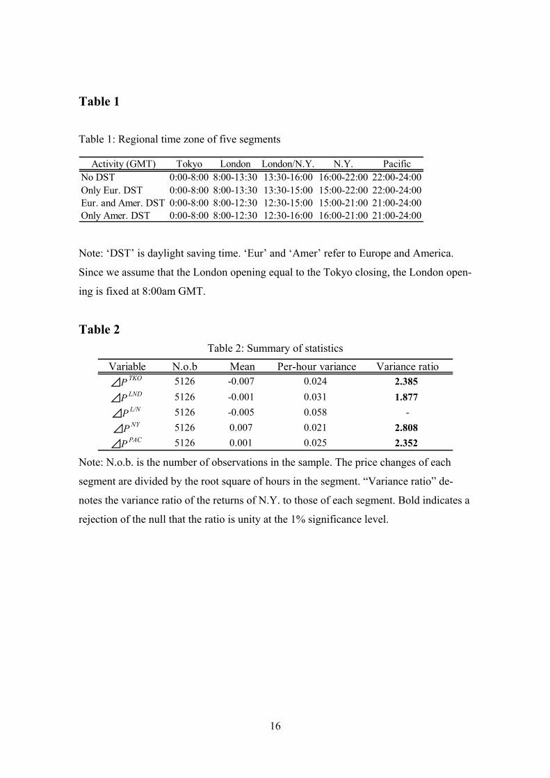
Table 1

Table 1: Regional time zone of five segments

Activity (GMT) Tokyo London London/N.Y. N.Y. PacificNo DST 0:00-8:00 8:00-13:30 13:30-16:00 16:00-22:00 22:00-24:00Only Eur. DST 0:00-8:00 8:00-13:30 13:30-15:00 15:00-22:00 22:00-24:00Eur. and Amer. DST 0:00-8:00 8:00-12:30 12:30-15:00 15:00-21:00 21:00-24:00Only Amer. DST 0:00-8:00 8:00-12:30 12:30-16:00 16:00-21:00 21:00-24:00

Note: ‘DST’ is daylight saving time. ‘Eur’ and ‘Amer’ refer to Europe and America.

Since we assume that the London opening equal to the Tokyo closing, the London open-

ing is fixed at 8:00am GMT.

Table 2 Table 2: Summary of statistics

Variable N.o.b Mean Per-hour variance Variance ratio⊿P TKO 5126 -0.007 0.024 2.385⊿P LND 5126 -0.001 0.031 1.877⊿P L/N 5126 -0.005 0.058 -⊿P NY 5126 0.007 0.021 2.808⊿P PAC 5126 0.001 0.025 2.352

Note: N.o.b. is the number of observations in the sample. The price changes of each

segment are divided by the root square of hours in the segment. “Variance ratio” de-

notes the variance ratio of the returns of N.Y. to those of each segment. Bold indicates a

rejection of the null that the ratio is unity at the 1% significance level.

16

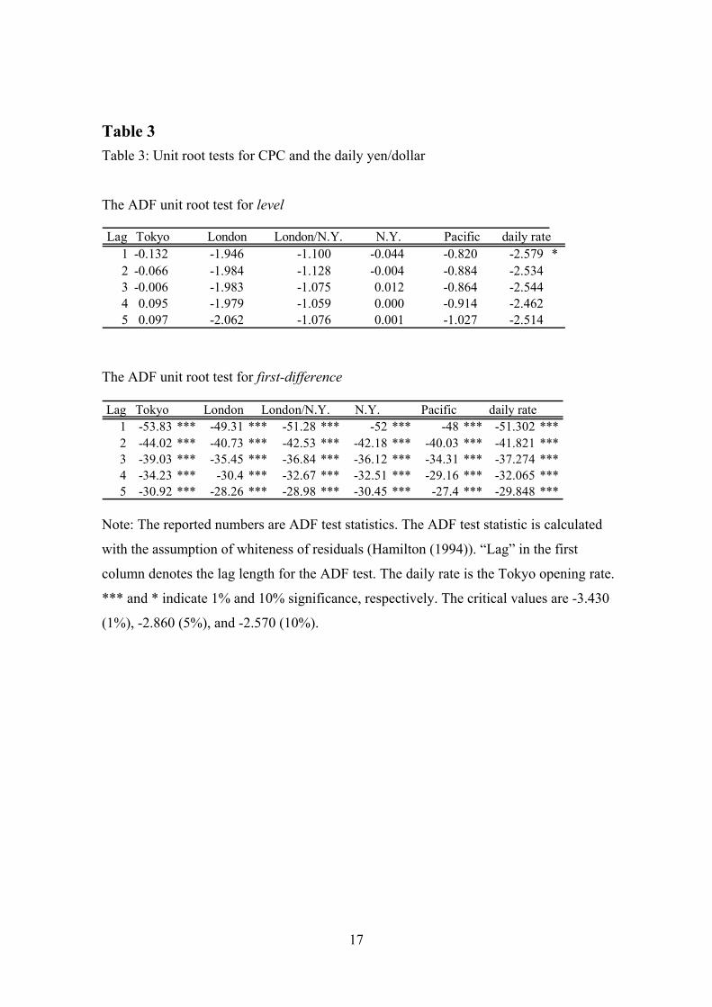
Table 3 Table 3: Unit root tests for CPC and the daily yen/dollar

The ADF unit root test for level

Lag Tokyo London London/N.Y. N.Y. Pacific daily rate1 -0.132 -1.946 -1.100 -0.044 -0.820 -2.5792 -0.066 -1.984 -1.128 -0.004 -0.884 -2.5343 -0.006 -1.983 -1.075 0.012 -0.864 -2.544

*

4 0.095 -1.979 -1.059 0.000 -0.914 -2.4625 0.097 -2.062 -1.076 0.001 -1.027 -2.514

The ADF unit root test for first-difference

Lag Tokyo London London/N.Y. N.Y. Pacific daily rate1 -53.83 *** -49.31 *** -51.28 *** -52 *** -48 *** -51.302 ***2 -44.02 *** -40.73 *** -42.53 *** -42.18 *** -40.03 *** -41.821 ***3 -39.03 *** -35.45 *** -36.84 *** -36.12 *** -34.31 *** -37.274 ***4 -34.23 *** -30.4 *** -32.67 *** -32.51 *** -29.16 *** -32.065 ***5 -30.92 *** -28.26 *** -28.98 *** -30.45 *** -27.4 *** -29.848 ***

Note: The reported numbers are ADF test statistics. The ADF test statistic is calculated

with the assumption of whiteness of residuals (Hamilton (1994)). “Lag” in the first

column denotes the lag length for the ADF test. The daily rate is the Tokyo opening rate.

*** and * indicate 1% and 10% significance, respectively. The critical values are -3.430

(1%), -2.860 (5%), and -2.570 (10%).

17

Table 4 Table 4: ADF cointegration test

Lag Tokyo London London/N.Y. N.Y. Pacific1 -2.363 -2.304 -2.883 ** -2.559 -2.5312 -2.367 -2.283 -2.871 ** -2.553 -2.5283 -2.337 -2.249 -2.850 * -2.524 -2.5044 -2.286 -2.194 -2.751 * -2.464 -2.4425 -2.360 -2.232 -2.844 * -2.523 -2.484

Note: The reported numbers are ADF test statistics. “Lag” in the first column is the lag

length for the ADF test. ** and * indicate 5 and 10% significance, respectively. The

critical values are -3.430 (1%), -2.860 (5%), and -2.570 (10%).

18

Table 5 Table 5: Testing for structural breaks

Segment Break dateModel C Tokyo 1993/03/09 -3.28

London 1992/09/11 -3.26London/N.Y. 2004/06/10 -3.57N.Y. 1993/03/09 -3.51Pacific 2002/05/23 -3.43

Minimum Phillips Z*t test statistic

Model C/S Tokyo 1993/01/27 -3.30London 1993/01/14 -3.22London/N.Y. 1996/05/09 -4.20N.Y. 1992/09/02 -4.24Pacific 1995/06/29 -4.24

Model C/S/T Tokyo 1995/10/20 -3.99London 1996/11/01 -3.68London/N.Y. 1998/10/13 -6.26 ***N.Y. 1990/10/19 -5.09Pacific 1995/08/14 -4.17

Note: Models C, C/S and C/S/T assume endogenous changes in intercept, inter-

cept/slope, and intercept/slope/trend, respectively. “Break date” refers to a possible

structural break point in a cointegration vector. “The minimum Philips Z*t test statistic”

corrects a bias due to a serial correlation of disturbance terms. *** indicates 1% signifi-

cance. The critical values (Gregory and Hansen, 1996a, b) are

Model C: -5.13 (1%), -4.61 (5%), -4.34 (10%).

Model C/S: -5.47 (1%), -4.95 (5%), -4.68 (10%).

Model C/S/T: -6.02 (1%), -5.50 (5%), -5.24 (10%).

19

Table 6

Table 6: Variance ratio tests

Lag ic5

10

20

30 VR 0.65 1.02 0.95 0.85 1.46L=M -3.01 0.15 -0.50 -1.31 4.11Rank -2.32 0.42 0.37 -1.90 4.98Sign 1.84 1.96 2.65 -0.37 4.92

Statistics Tokyo London London/N.Y. N.Y. PacifVR 0.83 1.04 0.92 0.97 1.10

L=M -3.91 0.63 -2.20 -0.74 2.62Rank -3.50 0.82 -2.51 -1.24 2.86Sign -0.32 1.41 -0.84 -0.10 3.21

VR 0.78 1.08 0.91 0.92 1.20L=M -3.42 0.88 -1.62 -1.15 3.19Rank -2.79 0.88 -1.62 -1.51 3.76Sign 0.75 1.18 0.20 0.51 3.46

VR 0.69 1.08 0.92 0.90 1.33L=M -3.30 0.63 -1.00 -1.09 3.66Rank -2.61 0.59 -0.50 -1.57 4.50Sign 1.58 1.55 1.50 -0.03 4.11

Segment

Note: "VR" is the variance-ratio estimate. "L=M" is Lo and Mackinlay's (1988) het-

eroskedasticity-robust z-statistic. "Rank" and "Sign" are Wright's (2000) rank- (R2) and

signed-based (S1) statistics, respectively. Bold denotes statistical significance at the 5%

level. The critical value is based on Table 1 in Wright (2000)

20

Figure 1: Intraday trading volume pattern in the yen/dollar foreign exchange market

Note: This figure shows regional trading volumes for Tokyo, London, and N.Y. All

trading volumes are indexed to the average overall trading volume where 100 equal the

average overall trading volume per 1-min period over the whole sample. Regional

mnemonics are LN-LN (London and London), NY-NY (N.Y. and N.Y.), TY-TY (To-

kyo and Tokyo), LN-NY (London and N.Y.), LN-TY (London and Tokyo), and NY-TY

(N.Y. and Tokyo).

Citation: Cai et al. (2007)

21

Figure 2-1: The Tokyo CPC (solid line) and the daily yen/dollar rate (dotted line)

Figure 2-2: The London CPC (solid line) and the daily yen/dollar rate (dotted line)

0

20

40

60

80

100

120

140

160

180

1987/9/14

1989/2/8

1990/7/5

1991/11/29

1993/4/27

1994/9/20

1996/2/15

1997/7/11

1998/12/7

2000/5/2

2001/9/26

2003/2/21

2004/7/19

2005/12/12

2007/5/9

-50

-40

-30

-20

-10

0

10

20

30

40

0

20

40

60

80

100

120

180

1987/9/14

1989/2/8

1990/7/5

1991/11/29

1993/4/27

1994/9/20

1996/2/15

1997/7/11

1998/12/7

2000/5/2

2001/9/26

2003/2/21

2004/7/19

2005/12/12

2007/5/9

-50

-40

-30

-20

-10

0

10

40

140

160

20

30

22

Figure 2-3: The London/N.Y. CPC (solid line) and the daily yen/dollar rate (dotted line)

Figure 2-4

: The N.Y. CPC (solid line) and the daily yen/dollar rate (dotted line)

0

20

40

60

80

100

120

140

160

180

1987/9/1

1989/2/8

1990/7/5

1991/11/

1993/4/2

1994/9/2

1996/2/1

1997/7/1

1998/12/

2000/5/2

2001/9/2

2003/2/2

2004/7/1

2005/12/

2007/5/9

-5

-4

-3

-2

-1

0

10

20

30

40

4 29

7 0 5 1 7 6 1 9 12

0

0

0

0

0

0

20

40

60

80

100

120

140

160

1801987/9/14

1989/2/8

1990/7/5

1991/11/29

1993/4/27

1994/9/20

1996/2/15

1997/7/11

1998/12/7

2000/5/2

2001/9/26

2003/2/21

2004/7/19

2005/12/12

2007/5/9

-50

-40

-30

-20

-10

0

10

20

30

40

23

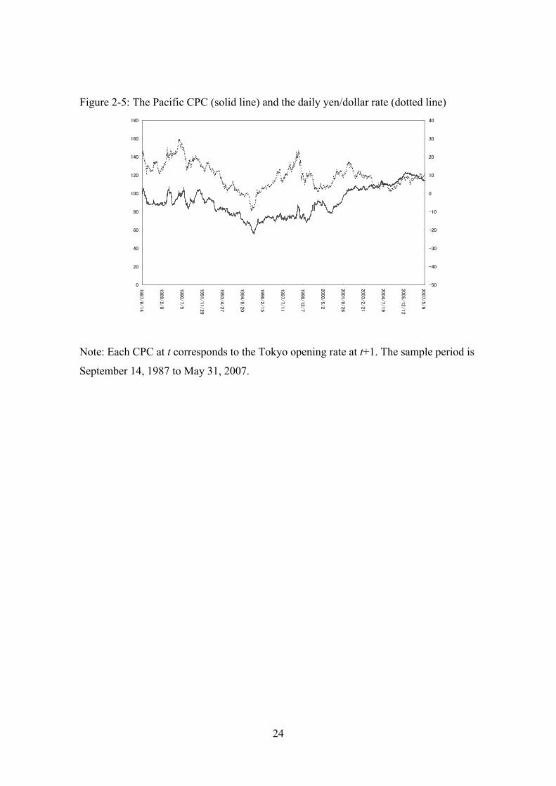
Figure 2-5: The Pacific CPC (solid line) and the daily yen/dollar rate (dotted line)

Note: Each CPC at t corresponds to the Tokyo opening rate at t+1. The sa

mple period is

eptember 14, 1987 to May 31, 2007.

0

20

40

60

80

100

120

140

160

180

1987/9/14

1989/2/8

1990/7/5

1991/11/29

1993/4/27

1994/9/20

1996/2/15

1997/7/11

1998/12/7

2000/5/2

2001/9/26

2003/2/21

2004/7/19

2005/12/12

2007/5/9

-50

-40

-30

-20

-10

0

10

20

30

40

S

24

Figure 3 Figure 3-1: MSE Decomposition [Measure (11)]

0.00

0.05

0.10

0.15

0.20

0.25

0.30

0.35

1 31 61 91 121 151 181

Tokyo LondonLondon/N.Y. N.Y.Pacific

Figure 3-2: MSE Decomposition [Measure (12)]

0.00

0.05

0.10

0.15

0.20

0.25

0.30

0.35

1 31 61 91 121 151 181

Tokyo LondonLondon/N.Y. N.Y.Pacific

Note: These two figures are calculated with the measures (11) and (12).

),(5),...,(1)

PATYiCPC i

ktit =− − (

)((

CPCCPCMSECPCMSE

ii

ktit −∑ −

11)

)(

),cov()()()(

ktt

ji

ktit

jkt

jtj

ikt

it

jkt

jt

ikt

it

SSMSE

CPCCPCCPCCPCCPCCPCmeanCPCCPCmeanCPCCPCMSE

−

−−−−−

−

−−+−−+− ∑∑

.),(5),...,(1 ijPATYj ≠= (12)

0.40

25