This article was downloaded by: [Oklahoma State University]On: 08 October 2014, At: 08:54Publisher: RoutledgeInforma Ltd Registered in England and Wales Registered Number: 1072954 Registered office: Mortimer House,37-41 Mortimer Street, London W1T 3JH, UK

Applied Financial EconomicsPublication details, including instructions for authors and subscription information:http://www.tandfonline.com/loi/rafe20

Intertemporal relations between the market volatilityindex and stock index returnsGhulam Sarwar aa Department of Accounting and Finance , College of Business and Public Administration,California State University , San Bernardino , CA 92407-2393 , USAPublished online: 01 Feb 2012.

To cite this article: Ghulam Sarwar (2012) Intertemporal relations between the market volatility index and stock indexreturns, Applied Financial Economics, 22:11, 899-909, DOI: 10.1080/09603107.2011.629980

To link to this article: http://dx.doi.org/10.1080/09603107.2011.629980

PLEASE SCROLL DOWN FOR ARTICLE

Taylor & Francis makes every effort to ensure the accuracy of all the information (the “Content”) containedin the publications on our platform. However, Taylor & Francis, our agents, and our licensors make norepresentations or warranties whatsoever as to the accuracy, completeness, or suitability for any purpose of theContent. Any opinions and views expressed in this publication are the opinions and views of the authors, andare not the views of or endorsed by Taylor & Francis. The accuracy of the Content should not be relied upon andshould be independently verified with primary sources of information. Taylor and Francis shall not be liable forany losses, actions, claims, proceedings, demands, costs, expenses, damages, and other liabilities whatsoeveror howsoever caused arising directly or indirectly in connection with, in relation to or arising out of the use ofthe Content.

This article may be used for research, teaching, and private study purposes. Any substantial or systematicreproduction, redistribution, reselling, loan, sub-licensing, systematic supply, or distribution in anyform to anyone is expressly forbidden. Terms & Conditions of access and use can be found at http://www.tandfonline.com/page/terms-and-conditions

Applied Financial Economics, 2012, 22, 899–909

Intertemporal relations between the

market volatility index and stock

index returns

Ghulam Sarwar

Department of Accounting and Finance, College of Business and Public

Administration, California State University, San Bernardino,

CA 92407-2393, USA

E-mail: gasrawar@csusb.edu

We examine the intertemporal relationships between Chicago Board

Options Exchange (CBOE) market volatility index (VIX) and returns

of the S&P 100, 500 and 600 indexes among three subperiods during

1992–2011 to account for structural shifts in VIX and to investigate if the

role of VIX as an investor fear gauge and indicator of portfolio insurance

price has strengthened in periods of high market anxiety and turbulence.

We find a strong negative contemporaneous relation between daily

changes (innovations) in VIX and S&P 100, 500 and 600 returns. Our

results suggest that the strength of contemporaneous VIX-returns relation

depends on the mean and volatility regime of VIX, and that this relation is

much stronger when VIX is both high and more volatile. In fact, during

2004–2011, the negative contemporaneous VIX-returns relation was the

most dominating and the only significant relation. Our results also indicate

a strong asymmetric relation between daily stock market returns and

innovations in VIX, suggesting that VIX is more of a gauge of investor fear

and portfolio insurance price than investor positive sentiment. The

response of VIX to negative changes in market returns was the highest

during 2004–2011 when VIX was most volatile. This result is consistent

with rising portfolio insurance premiums in periods of high market anxiety

and turbulence.

Keywords: VIX; S&P 500 and 100 returns; investor fear gauge; portfo-

lio insurance price; asymmetric relationship

JEL Classification: G14; G19; G10

I. Introduction

The market volatility index (VIX) of the Chicago

Board Options Exchange (CBOE) has been dubbed

as the investor fear gauge since high levels of VIX

have coincided with high degrees of market turmoil

(Whaley, 2000). The VIX is a forward looking index

of the expected short-term (30 days) market volatility

as it represents a market consensus estimate of future

stock market return volatility (Fleming et al., 1995;

Banerjee et al., 2007). When CBOE first introduced

the volatility index VIX in 1993, the index was

constructed based on the volatilities implied in

options on the S&P 100 index. In 2003, CBOE

Applied Financial Economics ISSN 0960–3107 print/ISSN 1466–4305 online � 2012 Taylor & Francis 899http://www.tandfonline.com

http://dx.doi.org/10.1080/09603107.2011.629980

Dow

nloa

ded

by [

Okl

ahom

a St

ate

Uni

vers

ity]

at 0

8:54

08

Oct

ober

201

4

revamped the definition and calculation of VIX. Thenew VIX uses the options on the S&P 500 index andreflects a much larger range of options across strikeprices (Carr and Wu, 2006; CBOE, 2009). The CBOErenamed the old VIX as VXO and calculated the newVIX back to 1990. Whaley (2009) argues that sincethe S&P 500 index options market is dominated byhedgers who buy index put options when they areconcerned about a potential drop in the stock market,VIX is also an indicator of the price of portfolioinsurance. Thus, high levels of VIX reflect investoranxiety about a potential drop in the stock market.The CBOE started trading of VIX futures in March2004 and VIX options in 2006. The VIX value iscomputed and disseminated to the investors on a real-time basis just like the information on major stockmarket indexes.

The real-time VIX value offers portfolio managers,hedge fund managers and other investors an up-to-the-minute estimate of future 1-month stock marketvolatility in order to make informed asset allocationand portfolio insurance decisions. VIX options andfutures afford investors viable tools to hedge marketvolatility. Some investigators advocate the use of VIXas a stock market timing or options trading timingtool (Copeland and Copeland, 1999; Arak andMajid, 2006).

Much of the empirical research in the extant VIXliterature is based on VXO (old VIX) than on VIX(new VIX). Giot (2005) examines if high levels ofVXO indicate oversold markets and finds that futurereturns are always positive (negative) after very high(low) levels of VXO. Copeland and Copeland (1999)examine VXO as a market timing tool to shiftbetween the style and size portfolios, and reportthat large and value stocks earn high returns follow-ing high VXO values. Arak and Majid (2006)conclude that selling options when VXO levels arehigh provide potential profits. Dash and Moran(2005) show that VXO is negatively correlated tohedge fund returns and this correlation profile isasymmetric. Guo and Whitelaw (2006) find thatmarket returns are positively related to impliedvolatilities. Blair et al. (2001) demonstrate thatVXO contains nearly all relevant information aboutthe future realized volatility of index returns for bothin-sample and out-of-sample forecasting. Fleminget al. (1995) find a large negative contemporaneouscorrelation between VXO changes and S&P 100 indexreturns, suggesting an inverse relation between VXOand stock market prices. Guo and Wohar (2006) findsignificant structural breaks (regime shifts) in themean levels of VXO and VIX at three distinctperiods: pre-1992, 1992–1997 and post-1997. Hongand Stein (1999) and Daniel et al. (1998) find that

stock market returns may behave differently depend-

ing on the state of the market. Durand et al. (2011)

find that the market risk premium and the value

premium in the Fama and French three-factor model

are sensitive to the changes in VIX.This article contributes to the market volatility

literature by focusing on VIX rather than VXO. The

main objective of the study is to investigate if the role

of VIX as an investor fear gauge and indicator of

portfolio insurance price has strengthened during

periods of high market anxiety and turbulence. Since

the mean VIX value is shown to have significant

structural shifts since 1992 (Guo and Wohar, 2006), it

is quite possible that the relation between VIX and

stock market returns is also subject to similar

structural changes during periods of high market

anxiety and relative market calm (low market vola-

tility). We examine and compare the VIX-returns

relations among three distinct subperiods during

1992–2011 on the basis of the previous evidence of

structural shifts in the mean levels of VIX and the

latest evidence of structural changes in the relation

between VIX and market returns in this study. Our

study is similar in spirit to Fleming et al. (1995) and

Whaley (2000) who examined VXO and S&P 100

returns until 1992. Our study period starts from

where Whaley (2000) left, and it includes the time

period since February 2006 when both VIX futures

and options were actively traded on CBOE. None of

the previous studies examined relations between

VIX and stock market returns when either VIX

futures or both VIX futures and options were

available as viable instruments for hedging market

volatility. We examine the intertemporal relationships

between VIX and S&P 500 index, VIX and S&P 100

index and VIX and S&P 600 small index returns. The

S&P 100 index was included to provide a comparative

analysis of our results with those of previous empir-

ical studies even though the daily S&P 100 and 500

index returns are known to have nearly perfect

correlations (0.99 during 1992–2011). The S&P 600

small index returns were studied to find out if the

relations between VIX and market returns spread to

the market for small stocks in addition to the markets

for large stocks as reflected in the S&P 100 and 500

indexes.The rest of the article is organized as follows.

Section II discusses the major differences between

VIX and VXO (old VIX) market volatility indexes.

Section III describes the methods for examining the

intertemporal relationship between VIX and stock

market indexes and the sources of data. Section IV

discusses the results. The summary and conclusions

are provided in Section V.

900 G. Sarwar

Dow

nloa

ded

by [

Okl

ahom

a St

ate

Uni

vers

ity]

at 0

8:54

08

Oct

ober

201

4

II. CBOE VIX and VXO MarketVolatility Indexes

The VXO (old VIX) is based on the impliedvolatilities of eight near-the-money S&P 100 optionsestimated from the Black–Scholes (1973) and Merton(1973b) option pricing models (CBOE, 2009). Thecash-dividend adjusted binomial method is used toaccount for the American-style feature of the S&P100 options (Fleming et al., 1995). At the two nearestmaturities, the CBOE selects two call and two putoptions for each maturity at the two strike prices thatstraddle the underlying spot price (Carr and Wu,2006). The implied volatilities from these options arethen interpolated to obtain 1-month (22 trading days)at-the-money implied volatilities. Thus, VXO is anaverage of 30-day at-the-money Black–Scholesimplied volatilities. Carr and Wu suggest that VXOapproximates the volatility swap rate with a 30-daymaturity. However, a replicating portfolio of thevolatility swaps is difficult to construct.

The VIX (new VIX) volatility index is based onmarket prices of the S&P 500 index options at the twonearest maturities. The calculation of VIX involves amuch larger set of call and put options at manydifferent strike prices and is not dependent on anyparticular option pricing model. Thus, VIX capturesinformation from the whole volatility skew ratherthan the volatility implied by at-the-money options(CBOE, 2009). As such, VIX measures the market’sexpectation of 30-day volatility conveyed by S&P 500index option prices (CBOE, 2009). Since the S&P 500index option market is much more active and deepthan the S&P 100 index option market and the S&P500 index is widely viewed as a proxy for the overallUS stock market (Whaley, 2009), the VIX representsa timely and accurate consensus estimate of the futureshort-term market volatility. Carr and Wu (2006)argue that the VIX squared approximates a 30-dayvariance swap rate. Because variance swap contractson major equity indexes are actively traded in overthe counter market, a replicating portfolio of the VIXsquared payoffs is not difficult to construct. This easeof creating a replicating portfolio may have contrib-uted to the CBOE decision to launch VIX futures andoptions in March 2004 and February 2006, respec-tively, after introducing VIX in September 2003.

III. Research Methods and Data

We first examine the statistical properties of theVIX and stock index return series and estimate theautocorrelation coefficients and cross correlations

between VIX and stock market returns. Given theinformation on cross correlations and followingFleming et al. (1995), we then use the followingmultivariate regression to study the intertemporalrelationships between VIX changes and stock marketreturns:

DVt ¼ �þX

�s,iRs,tþi þ �jsjjRs,tj þ "t, i ¼ �j, . . . , j

ð1Þ

where DVt is the change in VIX at time t, Rs,tþi is thestock index return at time tþ i, |Rs,t| is the absolutestock index return at time t, �s,i is the regressioncoefficient of the relation between Rs,tþi and DVt,�|s| is the regression coefficient for |Rs,t|, � is theregression intercept, and "t is the error term. SinceSchwert (1989, 1990) and Fleming et al. (1995) findasymmetric contemporaneous relationship betweenstock market returns and expected volatility, thecoefficients �s,i and �|s| are jointly designed tomeasure the asymmetric relation between Rs,t

and DVt.Because VIX is known as the investor fear gauge,

we expect the regression coefficient �s,0 for thecontemporaneous relation between change in VIXand stock index returns to have a negative sign. TheCapital Asset Pricing Model (CAPM) models ofSharpe (1964), Lintner (1965) and Merton (1973a)predict that stock prices will fall as expected volatilityrises, a prediction consistent with negative �s,0 value.The discounted cash flow model of stock valuationwould suggest that, assuming expected cash flows areunaffected, a rise in expected market volatility willraise the discount rate for the cash flows which willlead to lower stock prices. Black (1976) and Christie(1982) suggest an inverse relationship between stockprices and changes in future volatility because a dropin stock prices increases leverage which causesexpected volatility to rise. Indeed, Fleming et al.(1995) and Banerjee et al. (2007) report a strongnegative association between stock market returnsand changes in future volatility.

Giot (2005) suggests that high levels of VIXindicate oversold stock markets which lead to apositive relationship between volatility changes andfuture stock market returns. Guo and Whitelaw(2006), French et al. (1987) and Fleming et al.(1995) also report positive relationship betweenchanges in market volatility and future stock returns.Guo and Wohar (2006) find that VIX is meanreverting which suggests that a strong negativecontemporaneous relation between VIX changesand stock market returns may be followed by apositive relation between VIX changes and past stockmarket returns. Given these results, we expect the

Intertemporal relations between the market volatility index and stock index returns 901

Dow

nloa

ded

by [

Okl

ahom

a St

ate

Uni

vers

ity]

at 0

8:54

08

Oct

ober

201

4

regression coefficients �s,i, which capture the relationbetween VIX changes and lead and lagged stockmarket returns, to have positive signs. The coefficient�|s| captures the effect of the size of stock returnmovements, regardless of the direction of returns, onthe contemporaneous VIX changes. Schwert (1990)and Fleming et al. (1995) report an asymmetricrelation between market volatility and stock marketreturns, implying that an increase in market volatilityfrom a negative stock market returns is expected to bemuch larger than the decrease in market volatilityfrom a similar positive stock market returns. Hence,we expect that the joint coefficient (�s,0� �|s|), whichrepresents the effect of negative returns on VIX, willbe significantly larger in magnitude than the jointcoefficient (�s,0þ�|s|), which reflects the effect ofpositive returns on VIX.

Guo and Wohar (2006) find that the mean levelsof VIX shift over time. Fleming et al. (1995) andCarr and Wu (2006) show significant autocorrela-tions in stock market returns and VIX changes. Wetest for and find evidence of autocorrelation andheteroscedasticity in the estimated residuals of VIXchanges and index returns. To account for theheteroscedasticity and autocorrelation problemsin estimated parameters and SEs, we estimateEquation 1 using Hansen’s (1982) method ofmoments estimator to obtain consistent regressioncoefficients and SEs.

The data for this study for the two marketvolatility indexes (VIX and VXO) and three stockmarket indexes (S&P 100, S&P 500 and S&P 600small) came from the CBOE web site. The data coverthe time period from 2 January 1992 to 30 June 2011and have a total of 4915 daily observations. The dailydata represent the closing values of VIX, VXO andstock market indexes. Guo and Wohar (2006)find that VIX has three distinct regimes: pre-1992,1992–1997 and post-1997. To conform to theseregimes (structural shifts) of VIX, we divide ourdata into 1992–1997 and 1998–2011 subperiods.In addition, we propose a third subperiod from26 March 2004 to 30 June 2011 to capture the timeperiod when VIX futures and VIX options (since24 February 2006) were available to hedge stockmarket volatility. It is possible that the tradingopportunities in VIX futures and options mightaffect the behaviour of VIX. The subperiod 2004–2011 also includes the year 2008 when stock marketexperienced a severe contraction and VIX reached itshighest value since 1990.

IV. Results

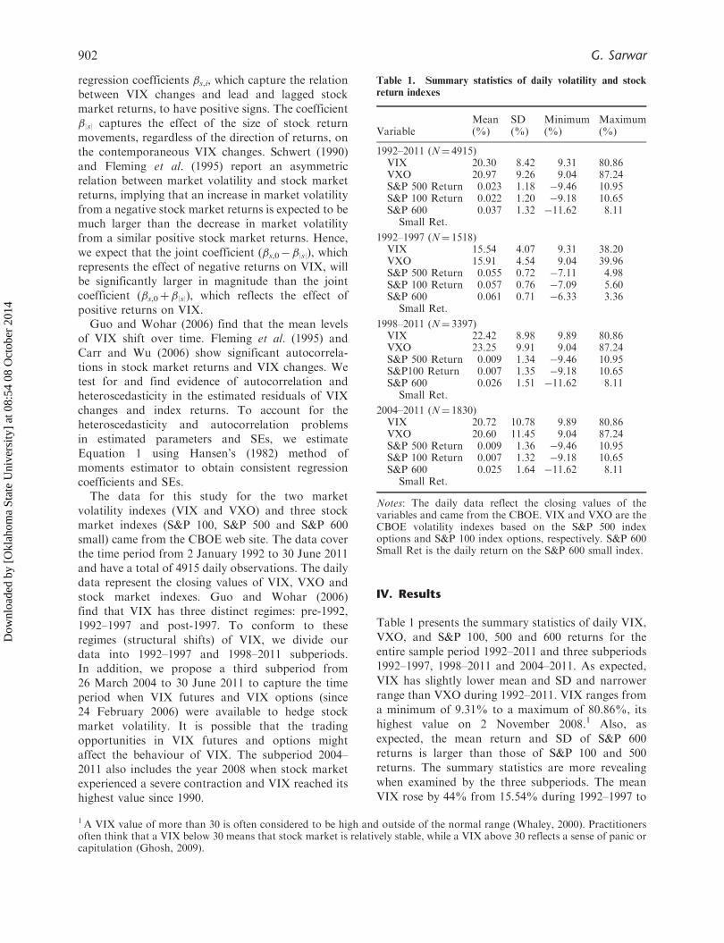
Table 1 presents the summary statistics of daily VIX,

VXO, and S&P 100, 500 and 600 returns for the

entire sample period 1992–2011 and three subperiods

1992–1997, 1998–2011 and 2004–2011. As expected,

VIX has slightly lower mean and SD and narrower

range than VXO during 1992–2011. VIX ranges from

a minimum of 9.31% to a maximum of 80.86%, its

highest value on 2 November 2008.1 Also, as

expected, the mean return and SD of S&P 600

returns is larger than those of S&P 100 and 500

returns. The summary statistics are more revealing

when examined by the three subperiods. The mean

VIX rose by 44% from 15.54% during 1992–1997 to

Table 1. Summary statistics of daily volatility and stock

return indexes

VariableMean(%)

SD(%)

Minimum(%)

Maximum(%)

1992–2011 (N¼ 4915)VIX 20.30 8.42 9.31 80.86VXO 20.97 9.26 9.04 87.24S&P 500 Return 0.023 1.18 �9.46 10.95S&P 100 Return 0.022 1.20 �9.18 10.65S&P 600

Small Ret.0.037 1.32 �11.62 8.11

1992–1997 (N¼ 1518)VIX 15.54 4.07 9.31 38.20VXO 15.91 4.54 9.04 39.96S&P 500 Return 0.055 0.72 �7.11 4.98S&P 100 Return 0.057 0.76 �7.09 5.60S&P 600

Small Ret.0.061 0.71 �6.33 3.36

1998–2011 (N¼ 3397)VIX 22.42 8.98 9.89 80.86VXO 23.25 9.91 9.04 87.24S&P 500 Return 0.009 1.34 �9.46 10.95S&P100 Return 0.007 1.35 �9.18 10.65S&P 600

Small Ret.0.026 1.51 �11.62 8.11

2004–2011 (N¼ 1830)VIX 20.72 10.78 9.89 80.86VXO 20.60 11.45 9.04 87.24S&P 500 Return 0.009 1.36 �9.46 10.95S&P 100 Return 0.007 1.32 �9.18 10.65S&P 600

Small Ret.0.025 1.64 �11.62 8.11

Notes: The daily data reflect the closing values of thevariables and came from the CBOE. VIX and VXO are theCBOE volatility indexes based on the S&P 500 indexoptions and S&P 100 index options, respectively. S&P 600Small Ret is the daily return on the S&P 600 small index.

1A VIX value of more than 30 is often considered to be high and outside of the normal range (Whaley, 2000). Practitionersoften think that a VIX below 30 means that stock market is relatively stable, while a VIX above 30 reflects a sense of panic orcapitulation (Ghosh, 2009).

902 G. Sarwar

Dow

nloa

ded

by [

Okl

ahom

a St

ate

Uni

vers

ity]

at 0

8:54

08

Oct

ober

201

4

22.42% during 1998–2011, while the SD of VIX(volatility of volatility) jumped by 121% from 4.07%to 8.98% during the same subperiods. The range ofVIX values was 70.97 percentage points during 1998–2011, compared to a VIX range of only 28.89percentage points during 1992–1997. These VIXsummary statistics corroborate with the findings ofGuo and Wohar (2006) that VIX experienced asignificant structural shift (regime change) from the1992–1997 period to the post-1997 period. In addi-tion, Table 1 shows that VIX experienced the largestdaily volatility during subperiod 2004–2011 whenboth VIX futures and options were traded. Like VIX,the mean and SD of stock index returns are alsosubstantially different between 1992–1997 and 1998–2011. The mean daily returns for both S&P 100 and500 indexes were only about 0.009% during 1998–2011, a period often referred to as the lost decade.Not only the mean daily returns for the S&P 100, 500and 600 indexes were two to six times larger in 1992–1997 than in 1998–2011, but also the SDs of thesestock index returns were 44% to 53% lower duringthis period relative to the period 1998–2011.

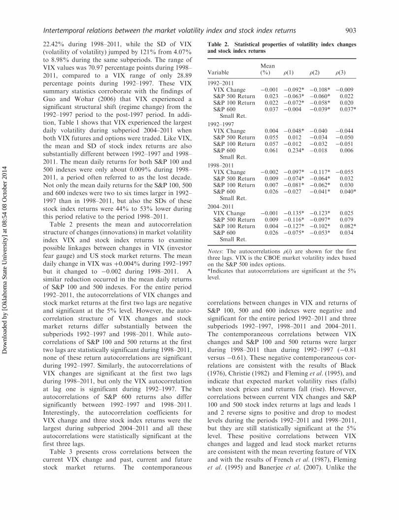
Table 2 presents the mean and autocorrelationstructure of changes (innovations) in market volatilityindex VIX and stock index returns to examinepossible linkages between changes in VIX (investorfear gauge) and US stock market returns. The meandaily change in VIX was þ0.004% during 1992–1997but it changed to �0.002 during 1998–2011. Asimilar reduction occurred in the mean daily returnsof S&P 100 and 500 indexes. For the entire period1992–2011, the autocorrelations of VIX changes andstock market returns at the first two lags are negativeand significant at the 5% level. However, the auto-correlation structure of VIX changes and stockmarket returns differ substantially between thesubperiods 1992–1997 and 1998–2011. While auto-correlations of S&P 100 and 500 returns at the firsttwo lags are statistically significant during 1998–2011,none of these return autocorrelations are significantduring 1992–1997. Similarly, the autocorrelations ofVIX changes are significant at the first two lagsduring 1998–2011, but only the VIX autocorrelationat lag one is significant during 1992–1997. Theautocorrelations of S&P 600 returns also differsignificantly between 1992–1997 and 1998–2011.Interestingly, the autocorrelation coefficients forVIX change and three stock index returns were thelargest during subperiod 2004–2011 and all theseautocorrelations were statistically significant at thefirst three lags.

Table 3 presents cross correlations between thecurrent VIX change and past, current and futurestock market returns. The contemporaneous

correlations between changes in VIX and returns ofS&P 100, 500 and 600 indexes were negative andsignificant for the entire period 1992–2011 and threesubperiods 1992–1997, 1998–2011 and 2004–2011.The contemporaneous correlations between VIXchanges and S&P 100 and 500 returns were largerduring 1998–2011 than during 1992–1997 (�0.81versus �0.61). These negative contemporaneous cor-relations are consistent with the results of Black(1976), Christie (1982) and Fleming et al. (1995), andindicate that expected market volatility rises (falls)when stock prices and returns fall (rise). However,correlations between current VIX changes and S&P100 and 500 stock index returns at lags and leads 1and 2 reverse signs to positive and drop to modestlevels during the periods 1992–2011 and 1998–2011,but they are still statistically significant at the 5%level. These positive correlations between VIXchanges and lagged and lead stock market returnsare consistent with the mean reverting feature of VIXand with the results of French et al. (1987), Fleminget al. (1995) and Banerjee et al. (2007). Unlike the

Table 2. Statistical properties of volatility index changes

and stock index returns

VariableMean(%) �(1) �(2) �(3)

1992–2011VIX Change �0.001 �0.092* �0.108* �0.009S&P 500 Return 0.023 �0.063* �0.060* 0.022S&P 100 Return 0.022 �0.072* �0.058* 0.020S&P 600

Small Ret.0.037 �0.004 �0.039* 0.037*

1992–1997VIX Change 0.004 �0.048* �0.040 �0.044S&P 500 Return 0.055 0.012 �0.034 �0.050S&P 100 Return 0.057 �0.012 �0.032 �0.051S&P 600

Small Ret.0.061 0.234* �0.018 0.006

1998–2011VIX Change �0.002 �0.097* �0.117* �0.055S&P 500 Return 0.009 �0.074* �0.064* 0.032S&P 100 Return 0.007 �0.081* �0.062* 0.030S&P 600

Small Ret.0.026 �0.027 �0.041* 0.040*

2004–2011VIX Change �0.001 �0.135* �0.123* 0.025S&P 500 Return 0.009 �0.116* �0.097* 0.079S&P 100 Return 0.004 �0.127* �0.102* 0.082*S&P 600

Small Ret.0.026 �0.075* �0.053* 0.034

Notes: The autocorrelations �(i) are shown for the firstthree lags. VIX is the CBOE market volatility index basedon the S&P 500 index options.*Indicates that autocorrelations are significant at the 5%level.

Intertemporal relations between the market volatility index and stock index returns 903

Dow

nloa

ded

by [

Okl

ahom

a St

ate

Uni

vers

ity]

at 0

8:54

08

Oct

ober

201

4

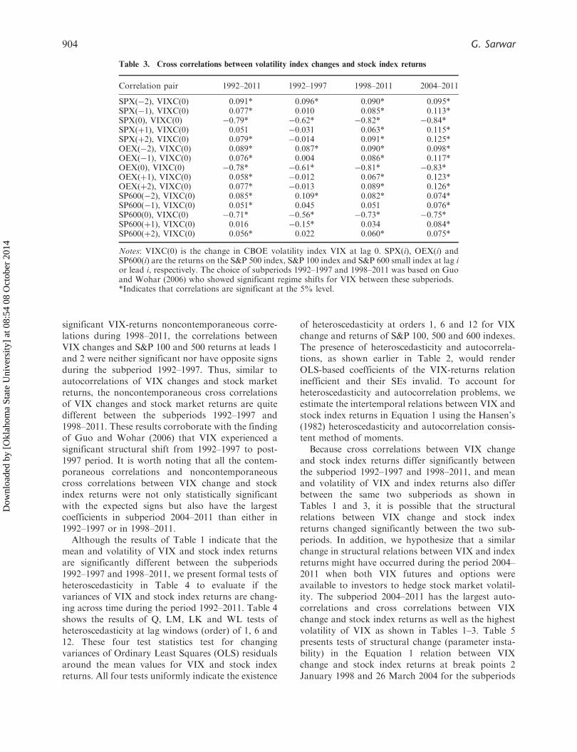
significant VIX-returns noncontemporaneous corre-lations during 1998–2011, the correlations betweenVIX changes and S&P 100 and 500 returns at leads 1and 2 were neither significant nor have opposite signsduring the subperiod 1992–1997. Thus, similar toautocorrelations of VIX changes and stock marketreturns, the noncontemporaneous cross correlationsof VIX changes and stock market returns are quitedifferent between the subperiods 1992–1997 and1998–2011. These results corroborate with the findingof Guo and Wohar (2006) that VIX experienced asignificant structural shift from 1992–1997 to post-1997 period. It is worth noting that all the contem-poraneous correlations and noncontemporaneouscross correlations between VIX change and stockindex returns were not only statistically significantwith the expected signs but also have the largestcoefficients in subperiod 2004–2011 than either in1992–1997 or in 1998–2011.

Although the results of Table 1 indicate that themean and volatility of VIX and stock index returnsare significantly different between the subperiods1992–1997 and 1998–2011, we present formal tests ofheteroscedasticity in Table 4 to evaluate if thevariances of VIX and stock index returns are chang-ing across time during the period 1992–2011. Table 4shows the results of Q, LM, LK and WL tests ofheteroscedasticity at lag windows (order) of 1, 6 and12. These four test statistics test for changingvariances of Ordinary Least Squares (OLS) residualsaround the mean values for VIX and stock indexreturns. All four tests uniformly indicate the existence

of heteroscedasticity at orders 1, 6 and 12 for VIXchange and returns of S&P 100, 500 and 600 indexes.The presence of heteroscedasticity and autocorrela-tions, as shown earlier in Table 2, would renderOLS-based coefficients of the VIX-returns relationinefficient and their SEs invalid. To account forheteroscedasticity and autocorrelation problems, weestimate the intertemporal relations between VIX andstock index returns in Equation 1 using the Hansen’s(1982) heteroscedasticity and autocorrelation consis-tent method of moments.

Because cross correlations between VIX changeand stock index returns differ significantly betweenthe subperiod 1992–1997 and 1998–2011, and meanand volatility of VIX and index returns also differbetween the same two subperiods as shown inTables 1 and 3, it is possible that the structuralrelations between VIX change and stock indexreturns changed significantly between the two sub-periods. In addition, we hypothesize that a similarchange in structural relations between VIX and indexreturns might have occurred during the period 2004–2011 when both VIX futures and options wereavailable to investors to hedge stock market volatil-ity. The subperiod 2004–2011 has the largest auto-correlations and cross correlations between VIXchange and stock index returns as well as the highestvolatility of VIX as shown in Tables 1–3. Table 5presents tests of structural change (parameter insta-bility) in the Equation 1 relation between VIXchange and stock index returns at break points 2January 1998 and 26 March 2004 for the subperiods

Table 3. Cross correlations between volatility index changes and stock index returns

Correlation pair 1992–2011 1992–1997 1998–2011 2004–2011

SPX(�2), VIXC(0) 0.091* 0.096* 0.090* 0.095*SPX(�1), VIXC(0) 0.077* 0.010 0.085* 0.113*SPX(0), VIXC(0) �0.79* �0.62* �0.82* �0.84*SPX(þ1), VIXC(0) 0.051 �0.031 0.063* 0.115*SPX(þ2), VIXC(0) 0.079* �0.014 0.091* 0.125*OEX(�2), VIXC(0) 0.089* 0.087* 0.090* 0.098*OEX(�1), VIXC(0) 0.076* 0.004 0.086* 0.117*OEX(0), VIXC(0) �0.78* �0.61* �0.81* �0.83*OEX(þ1), VIXC(0) 0.058* �0.012 0.067* 0.123*OEX(þ2), VIXC(0) 0.077* �0.013 0.089* 0.126*SP600(�2), VIXC(0) 0.085* 0.109* 0.082* 0.074*SP600(�1), VIXC(0) 0.051* 0.045 0.051 0.076*SP600(0), VIXC(0) �0.71* �0.56* �0.73* �0.75*SP600(þ1), VIXC(0) 0.016 �0.15* 0.034 0.084*SP600(þ2), VIXC(0) 0.056* 0.022 0.060* 0.075*

Notes: VIXC(0) is the change in CBOE volatility index VIX at lag 0. SPX(i), OEX(i) andSP600(i) are the returns on the S&P 500 index, S&P 100 index and S&P 600 small index at lag ior lead i, respectively. The choice of subperiods 1992–1997 and 1998–2011 was based on Guoand Wohar (2006) who showed significant regime shifts for VIX between these subperiods.*Indicates that correlations are significant at the 5% level.

904 G. Sarwar

Dow

nloa

ded

by [

Okl

ahom

a St

ate

Uni

vers

ity]

at 0

8:54

08

Oct

ober

201

4

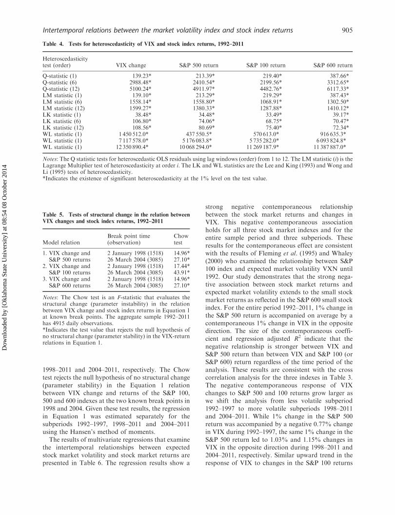
1998–2011 and 2004–2011, respectively. The Chowtest rejects the null hypothesis of no structural change(parameter stability) in the Equation 1 relationbetween VIX change and returns of the S&P 100,500 and 600 indexes at the two known break points in1998 and 2004. Given these test results, the regressionin Equation 1 was estimated separately for thesubperiods 1992–1997, 1998–2011 and 2004–2011using the Hansen’s method of moments.

The results of multivariate regressions that examinethe intertemporal relationships between expectedstock market volatility and stock market returns arepresented in Table 6. The regression results show a

strong negative contemporaneous relationshipbetween the stock market returns and changes inVIX. This negative contemporaneous associationholds for all three stock market indexes and for theentire sample period and three subperiods. Theseresults for the contemporaneous effect are consistentwith the results of Fleming et al. (1995) and Whaley(2000) who examined the relationship between S&P100 index and expected market volatility VXN until1992. Our study demonstrates that the strong nega-tive association between stock market returns andexpected market volatility extends to the small stockmarket returns as reflected in the S&P 600 small stockindex. For the entire period 1992–2011, 1% change inthe S&P 500 return is accompanied on average by acontemporaneous 1% change in VIX in the oppositedirection. The size of the contemporaneous coeffi-cient and regression adjusted R2 indicate that thenegative relationship is stronger between VIX andS&P 500 return than between VIX and S&P 100 (orS&P 600) return regardless of the time period of theanalysis. These results are consistent with the crosscorrelation analysis for the three indexes in Table 3.The negative contemporaneous response of VIXchanges to S&P 500 and 100 returns grow larger aswe shift the analysis from less volatile subperiod1992–1997 to more volatile subperiods 1998–2011and 2004–2011. While 1% change in the S&P 500return was accompanied by a negative 0.77% changein VIX during 1992–1997, the same 1% change in theS&P 500 return led to 1.03% and 1.15% changes inVIX in the opposite direction during 1998–2011 and2004–2011, respectively. Similar upward trend in theresponse of VIX to changes in the S&P 100 returns

Table 4. Tests for heteroscedasticity of VIX and stock index returns, 1992–2011

Heteroscedasticitytest (order) VIX change S&P 500 return S&P 100 return S&P 600 return

Q-statistic (1) 139.23* 213.39* 219.40* 387.66*Q-statistic (6) 2988.48* 2410.54* 2199.56* 3312.65*Q-statistic (12) 5100.24* 4911.97* 4482.76* 6117.33*LM statistic (1) 139.10* 213.29* 219.29* 387.43*LM statistic (6) 1558.14* 1558.80* 1068.91* 1302.50*LM statistic (12) 1599.27* 1380.33* 1287.88* 1410.12*LK statistic (1) 38.48* 34.48* 33.49* 39.17*LK statistic (6) 106.80* 74.06* 68.75* 70.47*LK statistic (12) 108.56* 80.69* 75.40* 72.34*WL statistic (1) 1 450 512.0* 437 550.5* 570 613.0* 916 635.3*WL statistic (1) 7 117 578.0* 5 176 083.8* 5 735 282.0* 6 093 824.8*WL statistic (1) 12 350 890.4* 10 068 294.0* 11 269 187.9* 11 387 887.0*

Notes: The Q statistic tests for heteroscedastic OLS residuals using lag windows (order) from 1 to 12. The LM statistic (i) is theLagrange Multiplier test of heteroscedasticity at order i. The LK andWL statistics are the Lee and King (1993) and Wong andLi (1995) tests of heteroscedasticity.*Indicates the existence of significant heteroscedasticity at the 1% level on the test value.

Table 5. Tests of structural change in the relation between

VIX changes and stock index returns, 1992–2011

Model relationBreak point time(observation)

Chowtest

1. VIX change andS&P 500 returns

2 January 1998 (1518) 14.96*26 March 2004 (3085) 27.10*

2. VIX change andS&P 100 returns

2 January 1998 (1518) 17.44*26 March 2004 (3085) 43.91*

3. VIX change andS&P 600 returns

2 January 1998 (1518) 14.96*26 March 2004 (3085) 27.10*

Notes: The Chow test is an F-statistic that evaluates thestructural change (parameter instability) in the relationbetween VIX change and stock index returns in Equation 1at known break points. The aggregate sample 1992–2011has 4915 daily observations.*Indicates the test value that rejects the null hypothesis ofno structural change (parameter stability) in the VIX-returnrelations in Equation 1.

Intertemporal relations between the market volatility index and stock index returns 905

Dow

nloa

ded

by [

Okl

ahom

a St

ate

Uni

vers

ity]

at 0

8:54

08

Oct

ober

201

4

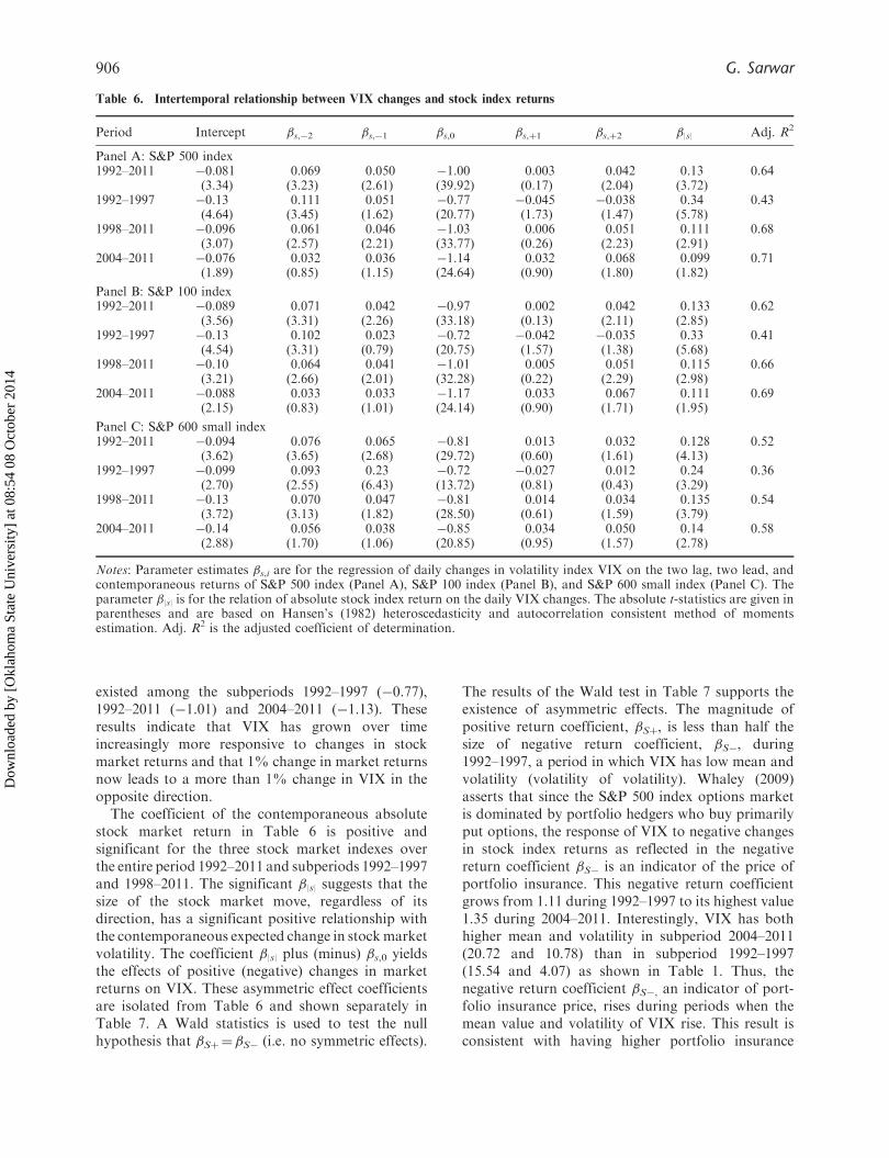
existed among the subperiods 1992–1997 (�0.77),1992–2011 (�1.01) and 2004–2011 (�1.13). Theseresults indicate that VIX has grown over timeincreasingly more responsive to changes in stockmarket returns and that 1% change in market returnsnow leads to a more than 1% change in VIX in theopposite direction.

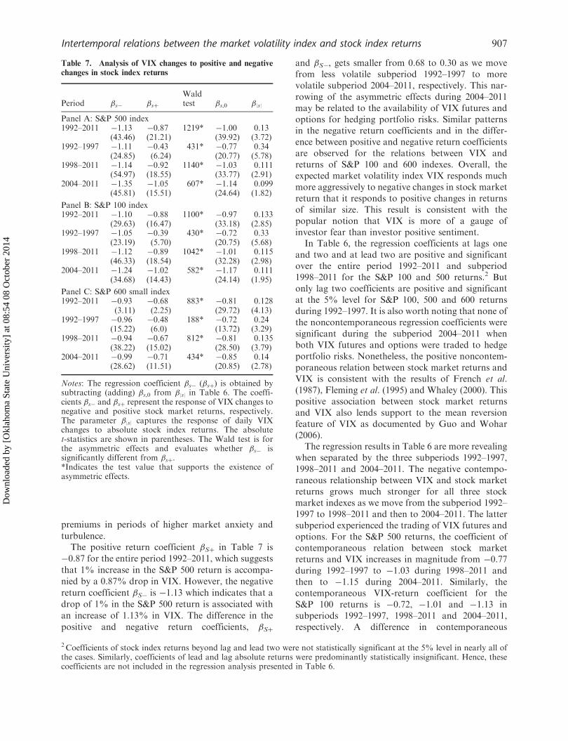
The coefficient of the contemporaneous absolutestock market return in Table 6 is positive andsignificant for the three stock market indexes overthe entire period 1992–2011 and subperiods 1992–1997and 1998–2011. The significant �|s| suggests that thesize of the stock market move, regardless of itsdirection, has a significant positive relationship withthe contemporaneous expected change in stockmarketvolatility. The coefficient �|s| plus (minus) �s,0 yieldsthe effects of positive (negative) changes in marketreturns on VIX. These asymmetric effect coefficientsare isolated from Table 6 and shown separately inTable 7. A Wald statistics is used to test the nullhypothesis that �Sþ¼�S� (i.e. no symmetric effects).

The results of the Wald test in Table 7 supports theexistence of asymmetric effects. The magnitude ofpositive return coefficient, �Sþ, is less than half thesize of negative return coefficient, �S�, during1992–1997, a period in which VIX has low mean andvolatility (volatility of volatility). Whaley (2009)asserts that since the S&P 500 index options marketis dominated by portfolio hedgers who buy primarilyput options, the response of VIX to negative changesin stock index returns as reflected in the negativereturn coefficient �S� is an indicator of the price ofportfolio insurance. This negative return coefficientgrows from 1.11 during 1992–1997 to its highest value1.35 during 2004–2011. Interestingly, VIX has bothhigher mean and volatility in subperiod 2004–2011(20.72 and 10.78) than in subperiod 1992–1997(15.54 and 4.07) as shown in Table 1. Thus, thenegative return coefficient �S�, an indicator of port-folio insurance price, rises during periods when themean value and volatility of VIX rise. This result isconsistent with having higher portfolio insurance

Table 6. Intertemporal relationship between VIX changes and stock index returns

Period Intercept �s,�2 �s,�1 �s,0 �s,þ1 �s,þ2 �|s| Adj. R2

Panel A: S&P 500 index1992–2011 �0.081 0.069 0.050 �1.00 0.003 0.042 0.13 0.64

(3.34) (3.23) (2.61) (39.92) (0.17) (2.04) (3.72)1992–1997 �0.13 0.111 0.051 �0.77 �0.045 �0.038 0.34 0.43

(4.64) (3.45) (1.62) (20.77) (1.73) (1.47) (5.78)1998–2011 �0.096 0.061 0.046 �1.03 0.006 0.051 0.111 0.68

(3.07) (2.57) (2.21) (33.77) (0.26) (2.23) (2.91)2004–2011 �0.076 0.032 0.036 �1.14 0.032 0.068 0.099 0.71

(1.89) (0.85) (1.15) (24.64) (0.90) (1.80) (1.82)

Panel B: S&P 100 index1992–2011 �0.089 0.071 0.042 �0.97 0.002 0.042 0.133 0.62

(3.56) (3.31) (2.26) (33.18) (0.13) (2.11) (2.85)1992–1997 �0.13 0.102 0.023 �0.72 �0.042 �0.035 0.33 0.41

(4.54) (3.31) (0.79) (20.75) (1.57) (1.38) (5.68)1998–2011 �0.10 0.064 0.041 �1.01 0.005 0.051 0.115 0.66

(3.21) (2.66) (2.01) (32.28) (0.22) (2.29) (2.98)2004–2011 �0.088 0.033 0.033 �1.17 0.033 0.067 0.111 0.69

(2.15) (0.83) (1.01) (24.14) (0.90) (1.71) (1.95)

Panel C: S&P 600 small index1992–2011 �0.094 0.076 0.065 �0.81 0.013 0.032 0.128 0.52

(3.62) (3.65) (2.68) (29.72) (0.60) (1.61) (4.13)1992–1997 �0.099 0.093 0.23 �0.72 �0.027 0.012 0.24 0.36

(2.70) (2.55) (6.43) (13.72) (0.81) (0.43) (3.29)1998–2011 �0.13 0.070 0.047 �0.81 0.014 0.034 0.135 0.54

(3.72) (3.13) (1.82) (28.50) (0.61) (1.59) (3.79)2004–2011 �0.14 0.056 0.038 �0.85 0.034 0.050 0.14 0.58

(2.88) (1.70) (1.06) (20.85) (0.95) (1.57) (2.78)

Notes: Parameter estimates �s,i are for the regression of daily changes in volatility index VIX on the two lag, two lead, andcontemporaneous returns of S&P 500 index (Panel A), S&P 100 index (Panel B), and S&P 600 small index (Panel C). Theparameter �|s| is for the relation of absolute stock index return on the daily VIX changes. The absolute t-statistics are given inparentheses and are based on Hansen’s (1982) heteroscedasticity and autocorrelation consistent method of momentsestimation. Adj. R2 is the adjusted coefficient of determination.

906 G. Sarwar

Dow

nloa

ded

by [

Okl

ahom

a St

ate

Uni

vers

ity]

at 0

8:54

08

Oct

ober

201

4

premiums in periods of higher market anxiety and

turbulence.The positive return coefficient �Sþ in Table 7 is

�0.87 for the entire period 1992–2011, which suggests

that 1% increase in the S&P 500 return is accompa-

nied by a 0.87% drop in VIX. However, the negative

return coefficient �S� is �1.13 which indicates that a

drop of 1% in the S&P 500 return is associated with

an increase of 1.13% in VIX. The difference in the

positive and negative return coefficients, �Sþ

and �S�, gets smaller from 0.68 to 0.30 as we movefrom less volatile subperiod 1992–1997 to morevolatile subperiod 2004–2011, respectively. This nar-rowing of the asymmetric effects during 2004–2011may be related to the availability of VIX futures andoptions for hedging portfolio risks. Similar patternsin the negative return coefficients and in the differ-ence between positive and negative return coefficientsare observed for the relations between VIX andreturns of S&P 100 and 600 indexes. Overall, theexpected market volatility index VIX responds muchmore aggressively to negative changes in stock marketreturn that it responds to positive changes in returnsof similar size. This result is consistent with thepopular notion that VIX is more of a gauge ofinvestor fear than investor positive sentiment.

In Table 6, the regression coefficients at lags oneand two and at lead two are positive and significantover the entire period 1992–2011 and subperiod1998–2011 for the S&P 100 and 500 returns.2 Butonly lag two coefficients are positive and significantat the 5% level for S&P 100, 500 and 600 returnsduring 1992–1997. It is also worth noting that none ofthe noncontemporaneous regression coefficients weresignificant during the subperiod 2004–2011 whenboth VIX futures and options were traded to hedgeportfolio risks. Nonetheless, the positive noncontem-poraneous relation between stock market returns andVIX is consistent with the results of French et al.(1987), Fleming et al. (1995) and Whaley (2000). Thispositive association between stock market returnsand VIX also lends support to the mean reversionfeature of VIX as documented by Guo and Wohar(2006).

The regression results in Table 6 are more revealingwhen separated by the three subperiods 1992–1997,1998–2011 and 2004–2011. The negative contempo-raneous relationship between VIX and stock marketreturns grows much stronger for all three stockmarket indexes as we move from the subperiod 1992–1997 to 1998–2011 and then to 2004–2011. The lattersubperiod experienced the trading of VIX futures andoptions. For the S&P 500 returns, the coefficient ofcontemporaneous relation between stock marketreturns and VIX increases in magnitude from �0.77during 1992–1997 to �1.03 during 1998–2011 andthen to �1.15 during 2004–2011. Similarly, thecontemporaneous VIX-return coefficient for theS&P 100 returns is �0.72, �1.01 and �1.13 insubperiods 1992–1997, 1998–2011 and 2004–2011,respectively. A difference in contemporaneous

Table 7. Analysis of VIX changes to positive and negative

changes in stock index returns

Period �s� �sþ

Waldtest �s,0 �|s|

Panel A: S&P 500 index1992–2011 �1.13 �0.87 1219* �1.00 0.13

(43.46) (21.21) (39.92) (3.72)1992–1997 �1.11 �0.43 431* �0.77 0.34

(24.85) (6.24) (20.77) (5.78)1998–2011 �1.14 �0.92 1140* �1.03 0.111

(54.97) (18.55) (33.77) (2.91)2004–2011 �1.35 �1.05 607* �1.14 0.099

(45.81) (15.51) (24.64) (1.82)

Panel B: S&P 100 index1992–2011 �1.10 �0.88 1100* �0.97 0.133

(29.63) (16.47) (33.18) (2.85)1992–1997 �1.05 �0.39 430* �0.72 0.33

(23.19) (5.70) (20.75) (5.68)1998–2011 �1.12 �0.89 1042* �1.01 0.115

(46.33) (18.54) (32.28) (2.98)2004–2011 �1.24 �1.02 582* �1.17 0.111

(34.68) (14.43) (24.14) (1.95)

Panel C: S&P 600 small index1992–2011 �0.93 �0.68 883* �0.81 0.128

(3.11) (2.25) (29.72) (4.13)1992–1997 �0.96 �0.48 188* �0.72 0.24

(15.22) (6.0) (13.72) (3.29)1998–2011 �0.94 �0.67 812* �0.81 0.135

(38.22) (15.02) (28.50) (3.79)2004–2011 �0.99 �0.71 434* �0.85 0.14

(28.62) (11.51) (20.85) (2.78)

Notes: The regression coefficient �s� (�sþ) is obtained bysubtracting (adding) �s,0 from �|s| in Table 6. The coeffi-cients �s� and �sþ represent the response of VIX changes tonegative and positive stock market returns, respectively.The parameter �|s| captures the response of daily VIXchanges to absolute stock index returns. The absolutet-statistics are shown in parentheses. The Wald test is forthe asymmetric effects and evaluates whether �s� issignificantly different from �sþ.*Indicates the test value that supports the existence ofasymmetric effects.

2 Coefficients of stock index returns beyond lag and lead two were not statistically significant at the 5% level in nearly all ofthe cases. Similarly, coefficients of lead and lag absolute returns were predominantly statistically insignificant. Hence, thesecoefficients are not included in the regression analysis presented in Table 6.

Intertemporal relations between the market volatility index and stock index returns 907

Dow

nloa

ded

by [

Okl

ahom

a St

ate

Uni

vers

ity]

at 0

8:54

08

Oct

ober

201

4

VIX-return coefficients of smaller magnitude over thethree subperiods was found for the S&P 600 returns.These results strongly suggest that negative relation-ship between market returns and VIX has changedsubstantially over time and that VIX is more than aunit responsive to a unit change in market returnsduring the latest 7-year period.

One important observation for the period 2004–2011 is that the negative contemporaneous associa-tion between stock market returns and VIX is theonly significant relationship that exists for all threeindexes during this period. In the latest 7-year period,one percentage point change in S&P 500 returnstriggers a 1.15 percentage point change in VIX in theopposite direction, compared to a VIX change ofonly 0.77 percentage point during the 5-year period1992–1997. The domination of negative contempora-neous relationship between stock market returns andVIX and the absence of noncontemporaneous effectsduring 2004–2011 may be related to the excessivelyhigh mean and volatility (volatility of volatility) ofVIX and the existence of VIX futures and options asviable tools for hedging market volatility during thelatest 7-year period.3

V. Summary and Conclusions

The CBOE market volatility index (VIX) is oftenused as an investor fear gauge and indicator ofportfolio insurance price. Most prior studies examinethe time series behaviour of VXO (old VIX) and itsrelation with different equity portfolio returns. Thisstudy examines the univariate time-series propertiesof VIX and the intertemporal relationships betweenVIX and returns of the S&P 100, 500 and 600 indexesfor the period 1992–2011. Because previous studiesshow evidence of structural shifts in VIX in the pre-and post-1997 periods and our study provide evi-dence of structural change in the VIX-returns relationat three different points during 1992–2011, we con-duct our analysis separately for subperiods 1992–1997, 1998–2011 and 2004–2011. The main objectiveof this study is to investigate if the role of VIX as aninvestor fear gauge and indicator of portfolio insur-ance price has strengthened during periods of highmarket anxiety and turbulence.

The results of cross correlation analysis indicatea strong negative contemporaneous relationshipbetween VIX and stock market returns.

This relationship is much stronger during 2004–2011 than during 1992–1997 and is followed andpreceded by positive noncontemporaneous relationbetween VIX and stock market returns. The regres-sion analyses suggest a strong negative contempora-neous relation between daily changes (innovations) inVIX and S&P 100, 500 and 600 returns during thethree subperiods. This negative contemporaneousrelationship grows much stronger in magnitudeas we shift analysis from low-volatility subperiod1992–1997 to high-volatility subperiod 2004–2011.The results suggest that the strength of contempora-neous VIX-returns relationship depends on the meanand volatility regime of VIX. The strongest concur-rent response of VIX to S&P 500 returns (�1.15) wasin subperiod 2004–2011 when VIX experienced thehighest volatility (i.e. high market anxiety) and when

both VIX futures and options were traded to hedgestock market volatility.

Our results also indicate a strong asymmetricrelation between daily stock market returns andinnovations in VIX in the subperiods 1992–1997,1998–2011 and 2004–2011. The VIX responds muchmore aggressively to negative changes in stock marketreturns than it responds to positive changes in returnsof similar size, suggesting that VIX is more of a gauge

of investor fear than investor positive sentiment. Thenegative return coefficient �S�, an indicator ofportfolio insurance price, rises during periods whenthe mean value and volatility of VIX rise and itreaches its highest value 1.35 in subperiod 2004–2011when VIX experienced the highest volatility. Thisresult is consistent with rising portfolio insurancepremiums in periods of higher market anxiety andturbulence.

References

Arak, M. and Majid, N. (2006) The VIX and VXNvolatility measures: fear gauges or forecasts,Derivatives Use, Trading and Regulation, 12, 14–27.

Banerjee, P. S., Doran, J. S. and Peterson, D. R. (2007)Implied volatility and future portfolio returns, Journalof Banking and Finance, 31, 3183–99.

Black, F. (1976) Studies of stock price volatility changes,in Proceedings of the 1976 Meetings of AmericanStatistical Association, Business and EconomicsSection, pp. 177–81.

Black, F. and Scholes, M. (1973) The pricing of options andcorporate liabilities, Journal of Political Economy, 81,637–54.

3We also conducted the regression analysis for the subperiod 24 February 2006 to 30 June 2011 when VIX options weretraded in addition to VIX futures which started trading on 26 March 2004. The regression analyses for this subperiod (notreported here) are virtually identical to those shown in Table 4 for 26 March 2004 to 30 June 2011 (i.e. 2004–2011).

908 G. Sarwar

Dow

nloa

ded

by [

Okl

ahom

a St

ate

Uni

vers

ity]

at 0

8:54

08

Oct

ober

201

4

Blair, B. J., Poon, S.-H. and Taylor, S. J. (2001)Forecasting S&P 100 volatility: the incremental infor-mation content of implied volatilities and high-frequency index returns, Journal of Econometrics,105, 5–17.

Carr, P. and Wu, L. (2006) A tale of two indices, TheJournal of Derivatives, 13, 13–29.

Chicago Board Options Exchange (CBOE) (2009)Available at http://www.cboe.com (accessed 15October 2011).

Christie, A. A. (1982) The stochastic behavior ofcommon stock variances: value, leverage, and inter-est rate effects, Journal of Financial Economics, 10,407–32.

Copeland, M. and Copeland, T. (1999) Market timing: styleand size rotation using the VIX, Financial AnalystsJournal, 55, 73–81.

Daniel, K., Hirshleifer, D. and Subrahmanyam, A. (1998)Investor psychology and investor security marketunder- and over-reaction, Journal of Finance, 53,189–209.

Dash, S. and Moran, M. T. (2005) VIX as a companion ofhedge fund portfolios, The Journal of AlternativeInvestments, 8, 75–82.

Durand, R. B., Lim, D. and Zumwalt, J. K. (2011) Fearand the Fama–French factors, Financial Management,40, 409–26.

Fleming, J., Ostdiek, B. and Whaley, R. E. (1995)Predicting stock market volatility: a new measure,Journal of Futures Markets, 15, 265–302.

French, K. R., Schwert, G. W. and Stambaugh, R. F.(1987) Expected stock returns and volatility,Journal of Financial Economics, 19, 3–29.

Ghosh, P. R. (2009) VIX’s actions trick market traditions,Wall Street Journal, 17 July.

Giot, P. (2005) Relationships between implied volatilityindexes and stock index returns, Journal of PortfolioManagement, 26, 12–17.

Guo, H. and Whitelaw, R. (2006) Uncovering the risk-neutral relationship in the stock market, Journal ofFinance, 61, 1433–63.

Guo, W. and Wohar, M. E. (2006) Identifying regimechanges in market volatility, The Journal of FinancialResearch, 29, 79–93.

Hansen, L. P. (1982) Large sample properties of generalizedmethod of moment estimators, Econometrica, 50,1029–54.

Hong, H. and Stein, J. (1999) A unified theory ofunderreaction, momentum trading, and overreactionin asset markets, Journal of Finance, 54, 2143–84.

Lee, J. H. and King, M. L. (1993) A locally most meanpowerful based score test for ARCH and GARCHregression disturbances, Journal of Business andEconomic Statistics, 11, 17–27.

Lintner, J. (1965) The valuation of risk assets and theselection of risky investments in stock portfolios andcapital budgets, Review of Economics and Statistics, 47,13–37.

Merton, R. C. (1973a) An intertemporal capital assetpricing model, Econometrica, 41, 867–88.

Merton, R. C. (1973b) Theory of rational option pricing,Bell Journal of Economics and Management Science, 4,141–83.

Schwert, G. W. (1989) Why does stock market volatilitychange over time?, Journal of Finance, 44, 1115–54.

Schwert, G. W. (1990) Stock volatility and crash of ‘87’,Review of Financial Studies, 3, 77–102.

Sharpe, W. F. (1964) Capital asset prices: a theory ofmarket equilibrium under conditions of risk, Journal ofFinance, 19, 425–42.

Whaley, R. E. (2000) The investor fear gauge, Journal ofPortfolio Management, 26, 12–17.

Whaley, R. E. (2009) Understanding the VIX, Journal ofPortfolio Management, 35, 98–105.

Wong, H. and Li, W. K. (1995) Postmanteau test forconditional heteroscedasticity using ranks of squaredresiduals, Journal of Applied Statistics, 22, 121–34.

Intertemporal relations between the market volatility index and stock index returns 909

Dow

nloa

ded

by [

Okl

ahom

a St

ate

Uni

vers

ity]

at 0

8:54

08

Oct

ober

201

4