NBER WORKING PAPER SERIES

AN INTERTEMPORAL CAPM WITH STOCHASTIC VOLATILITY

John Y. CampbellStefano Giglio

Christopher PolkRobert Turley

Working Paper 18411http://www.nber.org/papers/w18411

NATIONAL BUREAU OF ECONOMIC RESEARCH1050 Massachusetts Avenue

Cambridge, MA 02138September 2012

We are grateful to Torben Andersen, Gurdip Bakshi, John Cochrane, Bjorn Eraker, Bryan Kelly, IanMartin, Sydney Ludvigson, Monika Piazzesi, Ken Singleton, Tuomo Vuolteenaho, an Associate Editor,two anonymous referees, and seminar participants at various venues for comments. We thank JoshCoval, Ken French, Nick Roussanov, Mila Getmansky Sherman, and Tyler Shumway for providingdata used in the analysis. The views expressed herein are those of the authors and do not necessarilyreflect the views of the National Bureau of Economic Research.

At least one co-author has disclosed a financial relationship of potential relevance for this research.Further information is available online at http://www.nber.org/papers/w18411.ack

NBER working papers are circulated for discussion and comment purposes. They have not been peer-reviewed or been subject to the review by the NBER Board of Directors that accompanies officialNBER publications.

© 2012 by John Y. Campbell, Stefano Giglio, Christopher Polk, and Robert Turley. All rights reserved.Short sections of text, not to exceed two paragraphs, may be quoted without explicit permission providedthat full credit, including © notice, is given to the source.

An Intertemporal CAPM with Stochastic VolatilityJohn Y. Campbell, Stefano Giglio, Christopher Polk, and Robert TurleyNBER Working Paper No. 18411September 2012, Revised June 2015JEL No. G12,N22

ABSTRACT

This paper studies the pricing of volatility risk using the first-order conditions of a long-term equityinvestor who is content to hold the aggregate equity market rather than tilting towards value stocksand other equity portfolios that are attractive to short-term investors. We show that a conservativelong-term investor will avoid such tilts in order to hedge against two types of deterioration in investmentopportunities: declining expected stock returns, and increasing volatility. Empirically, we present novelevidence that low-frequency movements in equity volatility, tied to the default spread, are priced inthe cross-section of stock returns.

John Y. CampbellMorton L. and Carole S.Olshan Professor of EconomicsDepartment of EconomicsHarvard UniversityLittauer Center 213Cambridge, MA 02138and NBERjohn_campbell@harvard.edu

Stefano GiglioUniversity of ChicagoBooth School of Business5807 S. Woodlawn AvenueChicago, IL 60637and NBERstefano.giglio@chicagobooth.edu

Christopher PolkDepartment of FinanceLondon School of EconomicsHoughton St.London WC2A 2AEUKc.polk@lse.ac.uk

Robert TurleyHarvard UniversityBaker Library 220DBoston MA 02163robert.turley@dodgeandcox.com

A data appendix is available at:http://www.nber.org/data-appendix/w18411

1 Introduction

The fundamental insight of intertemporal asset pricing theory is that long-term investors

should care just as much about the returns they earn on their invested wealth as about the

level of that wealth. In a simple model with a constant rate of return, for example, the

sustainable level of consumption is the return on wealth multiplied by the level of wealth,

and both terms in this product are equally important. In a more realistic model with time-

varying investment opportunities, long-term investors with relative risk aversion greater than

one (conservative long-term investors) will seek to hold “intertemporal hedges”, assets that

perform well when investment opportunities deteriorate. Merton’s (1973) intertemporal

capital asset pricing model (ICAPM) shows that such assets should deliver lower average

returns in equilibrium if they are priced from conservative long-term investors’first-order

conditions.

Investment opportunities in the stock market may deteriorate either because expected

stock returns decline or because the volatility of stock returns increases. The relative

importance of these two types of intertemporal risk is an empirical question. In this paper,

we estimate an econometric model of stock returns that captures time-variation in both

expected returns and volatility and permits tractable analysis of long-term portfolio choice.

The model is a vector autoregression (VAR) for aggregate stock returns, realized variance,

and state variables, restricted to have scalar affi ne stochastic volatility so that the volatilities

of all shocks move proportionally.

Using this model and the first-order conditions of an infinitely-lived investor with Epstein-

Zin (1989, 1991) preferences, who is assumed to hold an aggregate stock index, we calculate

the risk aversion needed to make the investor content to hold the market index rather than

tilting his portfolio towards value stocks that offer higher average returns. We find that a

moderate level of risk aversion, around 7, is suffi cient to dissuade the investor from a tilt

towards value stocks. Growth stocks are attractive to a moderately conservative long-term

investor because they hedge against both declines in expected market returns and increases

1

in market volatility. These considerations would not be relevant for a single-period investor.

We obtain similar results for several other equity portfolio tilts, including tilts to portfolios

of stocks sorted by their past betas with market returns and with long-run volatility shocks,

and to managed portfolios that vary equity exposure in response to the level of expected

volatility. The major exception is that the conservative long-term investor would find it

attractive to hold a managed portfolio that varies equity exposure in response to time-

variation in expected stock returns. The reason is that we estimate only a weak correlation

between expected returns and volatility, so a market timing strategy does not lead to an

undesired volatility exposure.

Following Merton (1973), one might interpret the conservative long-term investor we

consider in this paper as a representative investor who trades freely in all asset markets.

There are however two obstacles to this interpretation. First, as already mentioned, our

model does not explain why such an agent would not vary equity exposure with the level

of the equity premium. Borrowing constraints can fix equity exposure at 100% when they

bind, but we estimate that they will not bind at all times in our historical sample. Second,

the aggregate stock index we consider here may not be an adequate proxy for all wealth,

a point emphasized by many papers including Campbell (1996), Jagannathan and Wang

(1996), Lettau and Ludvigson (2001), and Lustig, Van Nieuwerburgh, and Verdelhan (2013).

For both these reasons, we interpret our results in microeconomic terms, as a description

of the intertemporal considerations that limit the desire of conservative long-term equity

investors (including institutions such as pension funds and endowments) to follow value

strategies and other equity strategies with high average returns. These considerations

may contribute to the explanation of cross-sectional patterns in stock returns in a general

equilibrium setting with heterogeneous investors, even if they do not provide a complete

explanation in themselves.

Our empirical model provides a novel description of stochastic equity volatility that is of

independent interest. Our VAR system includes not only stock returns and realized vari-

2

ance, but also other financial indicators including the price-smoothed earnings ratio and the

default spread, the yield spread of low-rated over high-rated bonds. We find low-frequency

movements in volatility tied to these variables. While this phenomenon has received little

attention in the literature, we argue that it is a natural outcome of investor behavior. In-

vestors in risky bonds perceive the long-run component of volatility and incorporate this

information when they set credit spreads, as risky bonds are short the option to default

over long maturities. GARCH-based methods that filter only the information in past stock

returns fail to extract this low-frequency component of volatility, which is of key impor-

tance to long-horizon investors who care mostly about persistent changes in their investment

opportunity set.

The organization of our paper is as follows. Section 2 reviews related literature. Section

3 presents the first-order conditions of an infinitely-lived Epstein-Zin investor, allowing for a

specific form of stochastic volatility, and shows how they can be used to estimate preference

parameters. Section 4 presents data, econometrics, and VAR estimates of the dynamic

process for stock returns and realized volatility. This section documents the empirical suc-

cess of our model in forecasting long-run volatility. Section 5 introduces our test assets

and estimates their betas with news about the market’s future cash flows, discount rates,

and volatility. Section 6 turns to cross-sectional asset pricing and estimates the investor’s

preference parameters to fit a cross-section of excess returns on test assets, taking the dy-

namics of stock returns as given. This section also explores the implications of our model

for the history of our investor’s marginal utility. Section 7 concludes. An online appendix to

the paper (Campbell, Giglio, Polk, and Turley 2015a) provides supporting details including

a battery of robustness tests, and a companion paper (Campbell, Giglio, Polk, and Turley

2015b) considers non-equity test assets.

3

2 Literature Review

Since Merton (1973) first formulated the ICAPM, a large empirical literature has explored

the relevance of intertemporal considerations for the pricing of financial assets in general,

and the cross-sectional pricing of stocks in particular. One strand of this literature uses

the approximate accounting identity of Campbell and Shiller (1988a) and the first-order

conditions of an infinitely-lived investor with Epstein-Zin preferences to obtain approximate

closed-form solutions for the ICAPM’s risk prices (Campbell 1993). These solutions can be

implemented empirically if they are combined with vector autoregressive (VAR) estimates

of asset return dynamics. Campbell and Vuolteenaho (CV 2004), Campbell, Polk, and

Vuolteenaho (2010), and Campbell, Giglio, and Polk (CGP 2013) use this approach to argue

that value stocks outperform growth stocks on average because growth stocks hedge long-

term investors against declines in the expected return on the aggregate stock market.

A weakness of these papers is that they ignore time-variation in the volatility of stock

returns. We remedy this weakness by augmenting the VAR system with a scalar affi ne sto-

chastic volatility model, in which a single state variable governs the volatility of all shocks to

the VAR. In the continuous-time limit of the model, volatility always remains positive.2 We

extend the approximate closed-form ICAPM to allow for this type of stochastic volatility,

and derive three priced risk factors corresponding to three important attributes of aggregate

market returns: revisions in expected future cash flows, discount rates, and volatility.

An attractive feature of our model is that the prices of these three risk factors depend on

only one free parameter, the long-horizon investor’s coeffi cient of risk aversion. This protects

our empirical analysis from the critique of Daniel and Titman (1997, 2012) and Lewellen,

Nagel, and Shanken (2010) that models with multiple free parameters can spuriously fit the

returns to a set of test assets with a low-order factor structure. Our use of risk-sorted test

assets further protects us from this critique.

2Affi ne stochastic volatility models date back at least to Heston (1993) in continuous time. Similarmodels have been applied in the long-run risk literature by Eraker (2008) and Hansen (2012), among others,but much of this literature uses volatility specifications that are not guaranteed to remain positive.

4

Our work is complementary to recent research on the “long-run risk model”of asset prices

(Bansal and Yaron 2004) which can be traced back to insights in Kandel and Stambaugh

(1991). Both the approximate closed-form ICAPM and the long-run risk model start with

the first-order conditions of an infinitely-lived Epstein-Zin investor. As originally stated

by Epstein and Zin (1989), these first-order conditions involve both aggregate consumption

growth and the return on the market portfolio of aggregate wealth. Campbell (1993) pointed

out that the intertemporal budget constraint could be used to substitute out consumption

growth, turning the model into a Merton-style ICAPM. Restoy and Weil (1998, 2011) used

the same logic to substitute out the market portfolio return, turning the model into a gen-

eralized consumption CAPM in the style of Breeden (1979). Bansal and Yaron (2004)

added stochastic volatility to the Restoy-Weil model, and subsequent theoretical and em-

pirical research in the long-run risk framework has increasingly emphasized the importance

of stochastic volatility (Bansal, Kiku, and Yaron 2012, Beeler and Campbell 2012, Hansen

2012). In this paper, we give the approximate closed-form ICAPM the same ability to

handle stochastic volatility that its cousin, the long-run risk model, already possesses.3

Bansal, Kiku, Shaliastovich and Yaron (BKSY 2014), a paper written contemporaneously

with the first version of this paper, explores the effects of stochastic volatility in the long-

run risk model. Like us, they find stochastic volatility to be an important feature in the

time series of equity returns. An important difference is that BKSY’s benchmark model

assumes a homoskedastic process driving volatility. In our theoretical analysis, we discuss

some conditions that are required for their model solution to be valid and argue that these

conditions are not satisfied empirically. The different modeling assumptions and some

differences in empirical implementation account for our contrasting empirical results; we

show that volatility risk is very important in explaining the cross-section of stock returns

while they find it has little impact on cross-sectional differences in risk premia. Indeed,

BKSY find that a value-minus-growth bet has a positive beta with volatility news, while we

3Two unpublished papers by Chen (2003) and Sohn (2010) also attempt to do this. As we discuss in detailin the online appendix, these papers make strong assumptions about the covariance structure of various newsterms when deriving their pricing equations.

5

find it always has a negative volatility beta. Our negative volatility beta estimate is more

consistent with models of real options held by growth firms, such as McQuade (2012), and

with the underperformance of value stocks during periods of elevated volatility including the

Great Depression, the technology boom of the late 1990s, and the Great Recession of the

late 2000s (CGP 2013).

Stochastic volatility has been explored in other branches of the finance literature that we

summarize in the online appendix. Most obviously, this is a prime concern of the field of

financial econometrics. However, the focus has mostly been on univariate models, such as the

GARCH class of models (Engle 1982, Bollerslev 1986), or univariate filtering methods that

use realized high-frequency volatility (Barndorff-Nielsen and Shephard 2002, Andersen et al.

2003). A much smaller literature has, like us, looked directly at the information in other

economic and financial variables concerning future volatility (Schwert 1989, Christiansen,

Schmeling, and Schrimpf 2012, Paye 2012, Engle, Ghysels, and Sohn 2013).

3 An Intertemporal Model with Stochastic Volatility

In this section, we derive an expression for the log stochastic discount factor (SDF) of

the intertemporal CAPM model that allows for stochastic volatility. We then discuss the

properties of the model, including the requirements for a solution to exist, the implications

for asset pricing, and methods for estimation.

3.1 The stochastic discount factor

3.1.1 Preferences

We assume a representative agent with Epstein—Zin preferences and write the value function

as

6

Vt =[(1− δ)C

1−γθ

t + δ(Et[V 1−γt+1

])1/θ] θ1−γ

, (1)

where Ct is consumption and the preference parameters are the discount factor δ, risk aversion

γ, and the elasticity of intertemporal substitution (EIS) ψ. For convenience, we define

θ = (1− γ)/(1− 1/ψ).

The corresponding stochastic discount factor (SDF) can be written as

Mt+1 =

(δ

(CtCt+1

)1/ψ)θ (

Wt − CtWt+1

)1−θ

, (2)

where Wt is the market value of the consumption stream owned by the agent, including

current consumption Ct.4

We will be studying risk premia and are therefore concerned with innovations in the SDF.

We will also assume that asset returns and the SDF are conditionally jointly lognormally

distributed. Since we allow for changing conditional moments, we are careful to write both

first and second moments with time subscripts to indicate that they can vary over time.

Defining the log return on wealth rt+1 = ln (Wt+1/ (Wt − Ct)), and the log consumption-

wealth ratio ht+1 = ln (Wt+1/Ct+1) (denoted by h because this is the variable that determines

intertemporal hedging demand), we can write the innovation in the log SDF as

mt+1 − Etmt+1 = − θψ

(∆ct+1 − Et∆ct+1) + (θ − 1) (rt+1 − Etrt+1)

=θ

ψ(ht+1 − Etht+1)− γ(rt+1 − Etrt+1). (3)

The second equality uses the identity rt+1 − Etrt+1 = (∆ct+1 − Et∆ct+1) + (ht+1 − Etht+1)

to substitute consumption out of the SDF, replacing it with the wealth-consumption ratio

and the log return on the wealth portfolio.

4This notational convention is not consistent in the literature. Some authors exclude current consumptionfrom the definition of current wealth.

7

3.1.2 Solving the SDF forward

The online appendix shows that by using equation (3) to price the wealth portfolio, and

taking a loglinear approximation of the wealth portfolio return (that is perfectly accurate

when the elasticity of intertemporal substitution equals one), we obtain a difference equation

for the innovation in ht+1 that can be solved forward to an infinite horizon to obtain:

ht+1 − Etht+1 = (ψ − 1)(Et+1 − Et)∞∑j=1

ρjrt+1+j

+1

2

ψ

θ(Et+1 − Et)

∞∑j=1

ρjVart+j [mt+1+j + rt+1+j]

= (ψ − 1)NDR,t+1 +1

2

ψ

θNRISK,t+1, (4)

where ρ is a parameter of loglinearization related to the average consumption-wealth ratio,

and somewhat less than one. The second equality in (4) follows CV (2004) and uses the

notation NDR (“news about discount rates”) for revisions in expected future returns. In a

similar spirit, we write revisions in expectations of future risk (the variance of the future log

return plus the log stochastic discount factor) as NRISK .

Substituting (4) into (3) and simplifying, we obtain:

mt+1 − Etmt+1 = −γ [rt+1 − Etrt+1]− (γ − 1)NDR,t+1 +1

2NRISK,t+1

= −γNCF,t+1 − [−NDR,t+1] +1

2NRISK,t+1. (5)

The first equality in (5) expresses the log SDF in terms of the market return and news about

future variables. In particular, it identifies three priced factors: the market return (with

a price of risk γ), discount rate news (with price of risk (γ − 1)), and news about future

risk (with price of risk of −12). This is an extension of the ICAPM as derived by Campbell

(1993), with no reference to consumption or the elasticity of intertemporal substitution ψ.5

5Campbell (1993) briefly considers the heteroskedastic case, noting that when γ = 1, Vart [mt+1 + rt+1]is a constant. This implies that NRISK does not vary over time so the stochastic volatility term disappears.

8

The second equality rewrites the model, following CV (2004), by breaking the market

return into cash-flow news and discount-rate news. Cash-flow news NCF,t+1 is defined by

NCF,t+1 = rt+1−Etrt+1 + NDR,t+1. The price of risk for cash-flow news is γ times greater

than the unit price of risk for (negative) discount-rate news, hence CV call betas with cash-

flow news “bad betas”and those with negative discount-rate news “good betas”. The third

term in (5) shows the risk price for exposure to news about future risks and did not appear

in CV’s model, which assumed homoskedasticity. Not surprisingly, the model implies that

an asset providing positive returns when risk expectations increase will offer a lower return

on average; equivalently, the log SDF is high when future volatility is anticipated to be high.

Because the elasticity of intertemporal substitution (EIS) has no effect on risk prices in

our model, we do not identify this parameter and therefore do not face the recent critique of

Epstein, Farhi, and Strzalecki (2014) that models with a large wedge between risk aversion

and the reciprocal of the EIS imply an unrealistic willingness to pay for early resolution

of uncertainty.6 However, the EIS does influence the implied behavior of the investor’s

consumption, a topic we explore further below.

3.1.3 From news about risk to news about volatility

The risk news term NRISK,t+1 in equation (5) represents news about the conditional variance

of returns plus the stochastic discount factor, Vart [mt+1 + rt+1]. It therefore depends on the

SDF and its innovations. To close the model and derive its empirical implications, we must

make assumptions concerning the nature of the data generating process for stock returns

and the variance terms that will allow us to solve for Vart [mt+1 + rt+1] and NRISK,t+1.

Campbell claims that the stochastic volatility term also disappears when ψ = 1, but this is incorrect. Whenlimits are taken correctly, NRISK does not depend on ψ (except indirectly through the loglinearizationparameter, ρ).

6We use the standard terminology to describe the two parameters of the Epstein-Zin utility function, γ asrisk aversion and ψ as the elasticity of intertemporal substitution, although Garcia, Renault, and Semenov(2006) and Hansen, Heaton, Lee, and Roussanov (2007) point out that this interpretation may not be correctwhen γ differs from the reciprocal of ψ.

9

We assume that the economy is described by a first-order VAR

xt+1 = x̄ + Γ (xt − x̄) + σtut+1, (6)

where xt+1 is an n× 1 vector of state variables that has rt+1 as its first element, σ2t+1 as its

second element, and n−2 other variables that help to predict the first and second moments of

aggregate returns. x̄ and Γ are an n× 1 vector and an n×n matrix of constant parameters,

and ut+1 is a vector of shocks to the state variables normalized so that its first element

has unit variance. We assume that ut+1 has a constant variance-covariance matrix Σ, with

element Σ11 = 1. We also define n × 1 vectors e1 and e2, all of whose elements are zero

except for a unit first element in e1 and second element in e2.

The key assumption here is that a scalar random variable, σ2t , equal to the conditional

variance of market returns, also governs time-variation in the variance of all shocks to this

system. Both market returns and state variables, including variance itself, have innovations

whose variances move in proportion to one another. This assumption makes the stochastic

volatility process affi ne, as in Heston (1993). It implies that the conditional variance of

returns plus the stochastic discount factor is proportional to the conditional variance of

returns themselves.

Given this structure, news about discount rates can be written as

NDR,t+1 = e′1ρΓ (I− ρΓ)−1 σtut+1, (7)

while implied cash flow news is:

NCF,t+1 =(e′1 + e′1ρΓ(I− ρΓ)−1

)σtut+1. (8)

Our log-linear model makes the log SDF a linear function of the state variables, so

all shocks to the log SDF are proportional to σt, and Vart [mt+1 + rt+1] = ωσ2t for some

10

constant parameter ω. This implies that news about risk, NRISK , is proportional to news

about market return variance, NV :7

NRISK,t+1 = ωρe′2 (I− ρΓ)−1 σtut+1 = ωNV,t+1. (9)

The parameter ω is a nonlinear function of the coeffi cient of relative risk aversion γ, as

well as the VAR parameters and the loglinearization coeffi cient ρ, but it does not depend on

the elasticity of intertemporal substitution ψ except indirectly through the influence of ψ on

ρ. In the online appendix, we show that ω solves:

ωσ2t = (1− γ)2Vart [NCF,t+1] + ω(1− γ)Covt [NCF,t+1, NV,t+1] + ω2 1

4Vart [NV,t+1] . (10)

There are two main channels through which γ affects ω. First, a higher risk aversion–

given the underlying volatilities of all shocks– implies a more volatile stochastic discount

factor m, and therefore higher risk. This effect is proportional to (1 − γ)2, so it increases

rapidly with γ. Second, there is a feedback effect on current risk through future risk: ω

appears on the right-hand side of the equation as well. Given that in our estimation we find

Covt [NCF,t+1, NV,t+1] < 0, this second effect makes ω increase even faster with γ.

The quadratic equation (10) has two solutions, but the online appendix shows that one

of them can be disregarded. The false solution is easily identified by its implication that ω

becomes infinite as volatility shocks become small. The appendix also shows how to write

(10) directly in terms of the VAR parameters.

Finally, substituting (9) into (5), we obtain an empirically testable expression for the

7This property does not generally hold in the model with a homoskedastic process for σ2t proposed byBKSY (2014). In BKSY’s model, Vart(mt+1 + rt+1) is not in general proportional to σ2t , but depends onboth σ2t and σt. Therefore, NRISK is not in general proportional to NV , and NV is not in general the rightnews term to use in cross-sectional asset pricing. The online appendix shows that BKSY’s use of NV for assetpricing in this model can only be justified with additional special assumptions not stated by BKSY: thatNCF and NV are uncorrelated, and that the NV shock only depends on innovations of state variables whichare themselves homoskedastic. As these assumptions are inconsistent with the data, and the homoskedasticprocess allows σ2t to become negative even in continuous time, we do not further consider this model.

11

SDF innovations in the ICAPM with stochastic volatility:

mt+1 − Etmt+1 = −γNCF,t+1 − [−NDR,t+1] +1

2ωNV,t+1, (11)

where ω solves equation (10).

3.2 Properties and estimation of the model

3.2.1 Existence of a solution

With constant volatility, our model can be solved for any level of risk aversion, but in the

presence of stochastic volatility the model admits a solution only for values of risk aversion

consistent with the existence of a real solution to the quadratic equation (10). Given our VAR

estimates of the variance and covariance terms, the online appendix plots ω as a function of

γ and shows that a real solution for ω exists when γ lies between zero and 7.2.

The online appendix also shows that existence of a real solution for ω requires γ to satisfy

the upper bound:

γ ≤ 1− 1

(ρn − 1)σcfσv(12)

where ρn is the correlation between the news termsNCF andNV , σcf is the standard deviation

of the scaled cash-flow news NCF,t+1/σt, and σv is the standard deviation of the scaled

variance news NV,t+1/σt.

To develop the intuition behind these equations further, the online appendix studies a

simple example in which the link between the existence to a solution for equation (10) and

the existence of a value function for the representative agent can be shown analytically. The

example assumes ψ = 1, since we can then solve directly for the value function without

any need for a loglinear approximation of the return on the wealth portfolio (Tallarini 2000,

Hansen, Heaton, and Li 2008). In the example, we find that the condition for the existence of

the value function coincides precisely with the condition for the existence of a real solution

12

to the quadratic equation for ω. This result shows that the possible non-existence of a

solution to the quadratic equation for ω is a deep feature of the model, not an artifact

of our loglinear approximation to the wealth portfolio return– which is not needed in the

special case where ψ = 1. The problem arises because the value function becomes ever more

sensitive to volatility as the volatility of the value function increases, and this sensitivity

feeds back into the volatility of the value function, further increasing it. When this positive

feedback becomes too powerful, then the value function ceases to exist.8

In our empirical analysis, we take seriously the constraint implied by the quadratic equa-

tion (10), and require that our parameter estimates satisfy this constraint.9 Given the high

average returns to risky assets in historical data, this means in practice that our estimate of

risk aversion is often close to the estimated upper bound of 7.2.

3.2.2 Asset pricing equation and risk premia

To explore the implications of the model for risk premia, we use the general asset pricing

equation under conditional lognormality,

0 = ln Et exp{mt+1 + ri,t+1} = Et [mt+1 + ri,t+1] +1

2Vart [mt+1 + ri,t+1] . (13)

Combining this with the approximation

Etri,t+1 +1

2σ2it ' (EtRi,t+1 − 1) ,

8In the online appendix, we show that existence of the solution for ω also imposes a lower bound on γ:γ ≥ 1− (1/(ρn+1)σcfσv). We do not focus on this lower bound on γ since in our case it lies far below zero,at -6.8.

9The constraint is ignored in BKSY (2014), when they consider the case of time-varying volatility ofvolatility as a robustness test in their Sections II.E and III.D. There, rather than imposing that ω andγ satisfy equation (10), they linearize the equation so that a solution exists for all values of γ, allowingcombinations of (γ,ω) for which the true model does not have a solution. In the first draft of our paper wealso used this inappropriate linearization.

13

which links expected log returns (adjusted by one-half their variance) to expected gross level

returns Ri,t+1, and subtracting equation (13) for any reference asset j (which could be but

does not need to be a true risk-free rate) from the equation for asset i, we can write a moment

condition describing the relative risk premium of i relative to j as:

Et [Ri,t+1 −Rj,t+1 + (ri,t+1 − rj,t+1)(mt+1 − Etmt+1)]

= Et

[Ri,t+1 −Rj,t+1 − (ri,t+1 − rj,t+1)(γNCF,t+1 + [−NDR,t+1]− 1

2ωNV,t+1)

]= 0,(14)

where the second equality uses equation (11). This will be our main pricing equation: it

contains all conditional implications of the model, for any pair of assets i and j. We note that

in general the model does not restrict the covariances between the various assets’returns

and the news terms: these are taken as given in the data and not derived from the theory

(with the exception of the market portfolio itself, discussed in the next subsection).

We can alternatively write the moment conditions in covariance form:

Et [Ri,t+1 −Rj,t+1] = γCovt [ri,t+1 − rj,t+1, NCF,t+1]

+ Covt [ri,t+1 − rj,t+1,−NDR,t+1]− 1

2ωCovt [ri,t+1 − rj,t+1, NV,t+1] . (15)

As in CV (2004), this equation breaks an asset’s overall covariance with unexpected returns

on the wealth portfolio, rt+1−Etrt+1 = NCF,t+1−NDR,t+1, into two pieces, the first of which

has a higher risk price than the second whenever γ > 1. Importantly, it also adds a third

term capturing the asset’s covariance with shocks to long-run expected future volatility.

3.2.3 Conditional and unconditional implications of the model

The moment condition (14) summarizes the conditional asset pricing implications of the

model. It can be conditioned down to obtain the model’s unconditional implications, replac-

ing the conditional expectation in (14) with an unconditional expectation.

14

A special conditional implication of the model can be obtained when we focus on the

wealth portfolio and the real risk free rate Rf . In this case, since both rt+1 and mt+1 are

linear functions of the VAR state vector, their conditional covariance will be proportional to

the stochastic variance term σ2t :

Et [Rt+1 −Rf,t+1] = −Covt [rt+1,mt+1 − Etmt+1] ∝ σ2t (16)

The model implies that the risk premium on the market varies in proportion with the one-

period conditional variance of the market.

This conditional restriction has some implications for the relation between news terms,

in particular NDR and NV . While it does not tie the two terms precisely together (since

NDR also reflects news about the risk-free rate), it suggests that the two should be highly

correlated: news about high future variance should correspond to news about high future

discount rates. In the case that the risk-free rate is constant or at least unpredictable, the

model predicts NDR,t+1 ∝ NV,t+1.

In our empirical implementation, we do not impose this restriction on the VAR. One

reason for this is that we do not assume that we observe the riskless real return Rft+1. In

addition, a large literature has shown that empirically this restriction fails to hold when

standard empirical proxies for Rf,t+1 are used.10 Consistent with this, we find that our

empirical measure of σ2t , EVAR, does not significantly forecast returns in our unrestricted

VAR.

However, in our empirical analysis we do test conditional asset pricing implications of

the model by performing our GMM estimation using as instruments conditioning variables

implied by the model (specifically σ2t ). The only restriction we do not impose on the dynamics

of returns in the VAR is the counterfactual tight link between NDR and NV .

10See for example Campbell (1987), Harvey (1989, 1991), or the review in Lettau and Ludvigson (2010).

15

3.2.4 Estimation

Estimation via GMM is straightforward in this model given the moment representation of

the asset pricing equation (14). Conditional on the news terms, the model is a linear factor

model (with the caveat that both level and log returns appear), which is easy to estimate via

GMM even though it imposes nonlinear restrictions on the factor risk prices. The model has

only one free parameter, γ, that determines the risk prices as γ for NCF , 1 for −NDR, and

−ω(γ)/2 for NV , where ω(γ) is the solution of the quadratic equation (10) corresponding to

γ and the estimated news terms.

We estimate the VAR parameters and the news terms separately via OLS, and use GMM

to estimate the preference parameter γ. Our GMM standard errors for γ then condition on

the estimated news terms. In theory, it would be possible to estimate both the dynamics

and the moment conditions via GMM in one step. However, as discussed in CGP (2013),

this estimation is numerically involved and unstable given the large number of parameters.

The moment condition (14) holds for any two assets i and j. If a real risk-free rate were

available (which we would refer to as Rf), it would be a natural choice for the reference asset

j. In our empirical analysis, we use a nominal Treasury bill as the reference asset, writing

its return as RTbill, but we do not assume that this is a real riskless return. We do allow for

a free intercept relative to the Treasury bill return, as in Black’s (1972) implementation of

the CAPM, to account for the fact that investors are unable to borrow at the Treasury bill

rate but must typically pay a spread over this rate. The Treasury bill rate plus that spread

is the zero-beta rate of the intertemporal model.

Finally, we perform our GMM estimation using a prespecified diagonal weighting ma-

trix W whose elements are the inverse of the variances of the test assets. This approach

ensures that the GMM estimation is not focusing on some extreme linear combination of

the assets, while still taking into account the different variances of individual moment con-

ditions. We have repeated our analysis using one-step and two-step effi cient estimation, and

16

the qualitative results in the paper continue to hold in these cases.

3.2.5 Implied consumption innovations

As in Campbell (1993), we can estimate the model without having to observe the con-

sumption process of the investor. However, it is interesting to look at the model-implied

consumption, and compare it with the observed process of aggregate consumption.

Consumption innovations for our investor are given by

∆ct+1 − Et∆ct+1 = (rt+1 − Etrt+1)− (ψ − 1)NDR,t+1 − (ψ − 1)1

2

ω

1− γNV,t+1. (17)

The EIS parameter ψ, which enters this equation, is not pinned down by our VAR estima-

tion so we calibrate it to three different values, 0.5, 1.0, and 1.5. The online appendix shows

that implied consumption volatility is positively related to ψ, given our VAR estimates of

return dynamics. With ψ = 0.5, our investor’s consumption (which need not equal aggre-

gate consumption) is considerably more volatile than aggregate consumption but roughly as

volatile as equity dividend growth. Implied and actual consumption growth are positively

correlated, and more so when both series are exponentially smoothed.11

4 Predicting Aggregate Stock Returns and Volatility

4.1 State variables

Our full VAR specification of the vector xt+1 includes six state variables, four of which are

among the five variables in CGP (2013). To those four variables, we add the Treasury bill

11An interesting exercise would be to confront our implied consumption series with microeconomic dataon stockholders’consumption, as in Malloy, Moskowitz, and Vissing-Jørgensen (2009). However, the shortsample period over which such data are available is an obstacle to this approach.

17

rate RTbill (using it instead of the term yield spread used by CGP) and an estimate of

conditional volatility. The data are all quarterly, from 1926:2 to 2011:4.

The first variable in the VAR is the log real return on the market, rM , the difference

between the log return on the Center for Research in Securities Prices (CRSP) value-weighted

stock index and the log return on the Consumer Price Index. This is a standard proxy for

the aggregate wealth portfolio, but in the online appendix we consider alternative proxies

that delever the market return by combining it in various proportions with Treasury bills.

The second variable is expected market variance (EV AR). This variable is meant to

capture the variance of market returns, σ2t , conditional on information available at time

t, so that innovations to this variable can be mapped to the NV term described above.

To construct EV ARt, we proceed as follows. We first construct a series of within-quarter

realized variance of daily returns for each time t, RV ARt. We then run a regression of

RV ARt+1 on lagged realized variance (RV ARt) as well as the other five state variables at

time t. This regression then generates a series of predicted values for RV AR at each time

t + 1, that depend on information available at time t: ̂RV ARt+1. Finally, we define our

expected variance at time t to be exactly this predicted value at t+ 1:

EV ARt ≡ ̂RV ARt+1.

Note that though we describe our methodology in a two-step fashion where we first estimate

EV AR and then use EV AR in a VAR, this is only for interpretability. Indeed, this approach

to modelingEV AR can be considered a simple renormalization of equivalent results we would

find from a VAR that included RV AR directly.12

The third variable is the log of the S&P 500 price-smoothed earnings ratio (PE) adapted

from Campbell and Shiller (1988b), where earnings are smoothed over ten years. The variable

12Since we weight observations based on RV AR in the first stage and then reweight observations usingEV AR in the second stage, our two-stage approach in practice is not exactly the same as a one-stageapproach. However, the online appendix shows that results from a RV AR-weighted, single-step estimationare qualitatively very similar to those produced by our two-stage approach.

18

is constructed as in GCP (2013). The fourth is the yield on a three-month Treasury Bill

(RTbill) from CRSP. The fifth is the small-stock value spread (V S), constructed as described

in CGP (2013).

The sixth and final variable is the default spread (DEF ), defined as the difference between

the log yield on Moody’s BAA and AAA bonds, obtained from the Federal Reserve Bank

of St. Louis. We include the default spread in part because that variable is known to track

time-series variation in expected real returns on the market portfolio (Fama and French

1989), but also because shocks to the default spread should to some degree reflect news

about aggregate default probabilities, which in turn should reflect news about the market’s

future cash flows and volatility.

4.2 Short-run volatility estimation

In order for the regression model that generates EV ARt to be consistent with a reasonable

data-generating process for market variance, we deviate from standard OLS in two ways.

First, we constrain the regression coeffi cients to produce fitted values (i.e. expected market

return variance) that are positive. Second, given that we explicitly consider heteroskedas-

ticity of the innovations to our variables, we estimate this regression using Weighted Least

Squares (WLS), where the weight of each observation pair (RV ARt+1, xt) is initially based

on the time-t value of (RV AR)−1. However, to ensure that the ratio of weights across obser-

vations is not extreme, we shrink these initial weights towards equal weights. In particular,

we set our shrinkage factor large enough so that the ratio of the largest observation weight

to the smallest observation weight is always less than or equal to five. Though admittedly

somewhat ad hoc, this bound is consistent with reasonable priors on the degree of variation

over time in the expected variance of market returns. More importantly, we show in the

online appendix that our results are robust to variation in this bound. Both the constraint

on the regression’s fitted values and the constraint on WLS observation weights bind in the

sample we study.

19

The first-stage regression generating the state variable EV ARt is reported in Table 1,

Panel A. Perhaps not surprisingly, past realized variance strongly predicts future realized

variance. More importantly, the regression documents that an increase in either PE orDEF

predicts higher future realized volatility. Both of these results are strongly statistically signif-

icant and are a novel finding of the paper. The predictive power of very persistent variables

like PE and DEF indicates a potentially important role for lower-frequency movements in

stochastic volatility.

We argue that these empirical patterns are sensible. Investors in risky bonds incorporate

their expectation of future volatility when they set credit spreads, as risky bonds are short

the option to default. Therefore we expect higher DEF to predict higher RV AR. The

positive predictive relationship between PE and RV AR might seem surprising at first, but

one has to remember that the coeffi cient indicates the effect of a change in PE holding

constant the other variables, in particular the default spread DEF . Since the default spread

should also generally depend on the equity premium and since most of the variation in PE

is due to variation in the equity premium, we can regard PE as purging DEF of its equity

premium component to reveal more clearly its forecast of future volatility. We discuss this

interpretation further in section 4.4 below.

The R2 of the variance forecasting regression is nearly 38%. The relatively low R2 masks

the fact that the fit is indeed quite good, as we can see from Figure 1, in which RV AR and

EV AR are plotted together. The R2 is heavily influenced by occasional spikes in realized

variance, which the simple linear model we use is not able to capture. Indeed, our WLS

approach downweights the importance of these spikes in the estimation procedure.

20

4.3 Estimation of the VAR and the news terms

4.3.1 VAR estimates

We estimate a first-order VAR as in equation (6), where xt+1 is a 6 × 1 vector of state

variables ordered as follows:

xt+1 = [rM,t+1 EV ARt+1 PEt+1 RTbill,t+1 DEFt+1 V St+1]

so that the real market return rM,t+1 is the first element and EV AR is the second element. x̄

is a 6×1 vector of the means of the variables, and Γ is a 6×6 matrix of constant parameters.

Finally, σtut+1 is a 6×1 vector of innovations, with the conditional variance-covariance matrix

of ut+1 a constant Σ, so that the parameter σ2t scales the entire variance-covariance matrix

of the vector of innovations.

The first-stage regression forecasting realized market return variance described in the

previous section generates the variable EV AR. The theory in Section 3 assumes that σ2t ,

proxied for by EV AR, scales the variance-covariance matrix of state variable shocks. Thus,

as in the first stage, we estimate the second-stage VAR using WLS, where the weight of each

observation pair (xt+1, xt) is initially based on (EV ARt)−1. We continue to constrain both

the weights across observations and the fitted values of the regression forecasting EV AR.

Table 1, Panel B presents the results of the VAR estimation for the full sample (1926:2

to 2011:4). We report bootstrap standard errors for the parameter estimates of the VAR

that take into account the uncertainty generated by forecasting variance in the first stage.

Consistent with previous research, we find that PE negatively predicts future returns, though

the t-statistic indicates only marginal significance. The value spread has a negative but not

statistically significant effect on future returns. In our specification, a higher conditional

variance, EV AR, is associated with higher future returns, though the effect is not statistically

significant. Of course, the relatively high degree of correlation among PE, DEF , V S, and

21

EV AR complicates the interpretation of the individual effects of those variables. As for the

other novel aspects of the transition matrix, both high PE and high DEF predict higher

future conditional variance of returns. High past market returns forecast lower EV AR,

higher PE, and lower DEF .13

Table 1, Panel C reports the sample correlation matrices of both the unscaled residuals

σtut+1 and the scaled residuals ut+1. The correlation matrices report standard deviations

on the diagonals. A comparison of the standard deviations of the unscaled and scaled

residuals provides a rough indication of the effectiveness of our empirical solution to the

heteroskedasticity of the VAR. In general, the standard deviations of the scaled residuals are

several times larger than their unscaled counterparts. More specifically, our approach implies

that the scaled return residuals should have unit standard deviation. Our implementation

results in a sample standard deviation of 1.14.14

Table 1, Panel D reports the coeffi cients of a regression of the squared unscaled residuals

σtut+1 of each VAR equation on a constant and EV AR. These results are broadly consistent

with our assumption that EV AR captures the conditional volatility of the market return and

other state variables. The coeffi cient on EV AR in the regression forecasting the squared

market return residuals is 1.85, rather than the theoretically expected value of one, but this

coeffi cient is sensitive to the weighting scheme used in the regression. The fact that EV AR

significantly predicts with a positive sign all the squared errors of the VAR shows that the

volatilities of all innovations are driven by a common factor, as we assume, although of course

it is possible that empirically, other factors also influence the volatilities of certain variables.

13One worry is that many of the elements of the transition matrix are estimated imprecisely. Though theseestimates may be zero, their non-zero but statistically insignificant in-sample point estimates, in conjunctionwith the highly-nonlinear function that generates discount-rate and volatility news, may result in misleadingestimates of risk prices. However, the online appendix shows that results are qualitatively similar if weinstead employ a partial VAR where, via a standard iterative process, only variables with t-statistics greaterthan 1.0 are included in each VAR regression.14A comparison of the unscaled and scaled autocorrelation matrices, in the online appendix, reveals in ad-

dition that much of the sample autocorrelation in the unscaled residuals is eliminated by our WLS approach.

22

4.3.2 News terms

The top panel of Table 2 presents the variance-covariance matrix and the standard devia-

tion/correlation matrix of the news terms, estimated as described above. Consistent with

previous research, we find that discount-rate news is nearly twice as volatile as cash-flow

news.

The interesting new results in this table concern the variance news term NV . First,

news about future variance has significant volatility, with nearly a third of the variability of

discount-rate news. Second, variance news is negatively correlated (−0.12) with cash-flow

news: as one might expect from the literature on the “leverage effect”(Black 1976, Christie

1982), news about low cash flows is associated with news about higher future volatility.

This finding makes it unappealing to assume that variance news and cash-flow news are

uncorrelated, as would be required for the validity of the model solution in BKSY (2014).

Third, NV is close to uncorrelated (−0.03) with discount-rate news.15 The net effect of these

correlations, documented in the lower left panel of Table 2, is a slightly negative correlation

of −0.03 between our measure of volatility news and contemporaneous market returns.

The lower right panel of Table 2 reports the decomposition of the vector of innovations

σ2tut+1 into the three terms NCF,t+1, NDR,t+1, and NV,t+1. As shocks to EV AR are just a

linear combination of shocks to the underlying state variables, which includes RV AR, we

“unpack”EV AR to express the news terms as a function of rM , PE, RTbill, V S, DEF , and

RV AR. The panel shows that innovations to RV AR are mapped more than one-to-one to

news about future volatility. However, several of the other state variables also drive news

about volatility. Specifically, we find that innovations in PE, DEF , and V S are associated

with news of higher future volatility. This panel also indicates that all state variables with

the exception of RTbill are statistically significant in terms of their contribution to at least

one of the three news terms. We choose to leave RTbill in the VAR, though its presence in

15Though the point estimate of this correlation is negative, the large standard error implies that wecannot reject the “volatility feedback effect”(Campbell and Hentschel 1992, Calvet and Fisher 2007), whichgenerates a positive correlation. For related research see French, Schwert, and Stambaugh (1987).

23

the system makes little difference to our conclusions.

Figure 2 plots the smoothed series for NCF , −NDR and NV using an exponentially-

weighted moving average with a quarterly decay parameter of 0.08. This decay parameter

implies a half-life of approximately two years. The pattern of NCF and −NDR we find is

consistent with previous research. As a consequence, we focus on the smoothed series for

market variance news. There is considerable time variation in NV , and in particular we find

episodes of news of high future volatility during the Great Depression and just before the

beginning of World War II, followed by a period of little news until the late 1960s. From

then on, periods of positive volatility news alternate with periods of negative volatility news

in cycles of 3 to 5 years. Spikes in news about future volatility are found in the early 1970s

(following the oil shocks), in the late 1970s and again following the 1987 crash of the stock

market. The late 1990s are characterized by strongly negative news about future returns,

and at the same time higher expected future volatility. The recession of the late 2000s is

instead characterized by strongly negative cash-flow news, together with a spike in volatility

of the highest magnitude in our sample. The recovery from the financial crisis has brought

positive cash-flow news together with news about lower future volatility.

4.4 Predicting long-run volatility

The predictability of volatility, and especially of its long-run component, is central to this

paper. In the previous sections, we have shown that volatility is strongly predictable, specif-

ically by variables beyond lagged realizations of volatility itself: PE and DEF contain

essential information about future volatility. We have also proposed a VAR-based method-

ology to construct long-horizon forecasts of volatility that incorporate all the information in

lagged volatility as well as in the additional predictors like PE and DEF .

We now ask how well our proposed long-run volatility forecast captures the long-horizon

component of volatility. In the online appendix we regress realized, discounted, annualized

24

long-run variance up to period h,

LHRV ARh =4Σh

j=1ρj−1RV ARt+j

Σhj=1ρ

j−1,

on the variables included in our VAR system, the VAR long-horizon forecast, and some

alternative forecasts of long-run variance. We focus on a 10-year horizon (h = 40) as longer

horizons come at the cost of fewer independent observations; however, the online appendix

confirms that our results are robust to horizons ranging from one to 15 years.

As alternatives to the VAR approach, we estimate two standard GARCH-type models,

specifically designed to capture the long-run component of volatility: the two-component

exponential (EGARCH) model proposed by Adrian and Rosenberg (2008), and the frac-

tionally integrated (FIGARCH) model of Baillie, Bollerslev, and Mikkelsen (1996). We first

estimate both GARCH models using the full sample of daily returns and then generate the

appropriate forecast of LHRV AR40. To these two models, we add the set of variables from

our VAR, and compare the forecasting ability of these different models. We find that while

the EGARCH and FIGARCH forecasts do forecast long-run volatility, our VAR variables

provide as good or better explanatory power, and RV AR, PE and DEF are strongly sta-

tistically significant. Our long-run VAR forecast has a coeffi cient of 1.02, which remains

highly significant at 0.82 even in the presence of the FIGARCH forecast. We also find that

DEF does not predict long-horizon volatility in the presence of our VAR forecast, implying

that the VAR model captures the long-horizon information in the default spread.

The online appendix also examines more carefully the links between PE, DEF , and

LHRV AR40. We find that by itself, PE has almost no information about low-frequency

variation in volatility. In contrast,DEF forecasts nearly 22% of the variation in LHRV AR40.

And if we use the component ofDEF that is orthogonal to PE, which we callDEFO, the R2

increases to over 51%. Our interpretation of these results is that DEF contains information

about future volatility because risky bonds are short the option to default. However, DEF

also contains information about future aggregate risk premia. We know from previous work

25

that most of the variation in PE reflects aggregate risk premia. Therefore, including PE in

the volatility forecasting regression cleans up variation in DEF due to aggregate risk premia

and thus sharpens the link between DEF and future volatility. Since PE and DEF are

negatively correlated (default spreads are relatively low when the market trades rich), both

PE and DEF receive positive coeffi cients in the multiple regression.

Figure 3 provides a visual summary of the long-run volatility-forecasting power of our

key VAR state variables and our interpretation. The top panel plots LHRV AR40 together

with lagged DEF and PE. The graph confirms the strong negative correlation between PE

and DEF (correlation of -0.6) and highlights how both variables track long-run movements

in long run volatility. To isolate the contribution of the default spread in predicting long run

volatility, the bottom panel plots LHRV AR40 together with DEFO. The improvement in

fit moving from the top panel to the bottom panel is clear.

The contrasting behavior of DEF and DEFO in the two panels during episodes such

as the tech boom help illustrate the workings of our story. Taken in isolation, the relatively

stable default spread throughout most of the late 1990s would predict little change in future

market volatility. However, once the declining equity premium over that period is taken into

account (as shown by the rapid increase in PE), one recognizes that a PE-adjusted default

spread in the late 1990s actually forecasted much higher volatility ahead.

As a further check on the usefulness of our VAR approach, in the online appendix we

compare our variance forecasts to option-implied variance forecasts over the period 1998—

2011. We find that when both the VAR and option data are used to predict realized variance,

the VAR forecasts drive out the option-implied forecasts while remaining statistically and

economically significant.

Taken together, these results make a strong case that credit spreads and valuation ra-

tios contain information about future volatility not captured by simple univariate models,

even those designed to fit long-run movements in volatility, and that our VAR method for

calculating long-horizon forecasts preserves this information.

26

5 Test Assets and Beta Measurement

5.1 Test assets

In addition to the six VAR state variables, our analysis requires excess returns on a cross

section of test assets. We construct several sets of portfolios for this purpose, reporting

details on the construction method in the online appendix.

Our primary cross section consists of the excess returns over Treasury bills on the 25

ME- and BE/ME-sorted portfolios, studied in Fama and French (1993), extended in Davis,

Fama, and French (2000), and made available by Professor Kenneth French on his website.

We consider two main subsamples: early (1931:3-1963:3) and modern (1963:4-2011:4) due

to the findings in CV (2004) of important differences in the risks of these portfolios between

the early and modern period.

To guard against the concerns of Daniel and Titman (1997, 2012) and Lewellen, Nagel,

and Shanken (2010) that characteristic-sorted portfolios may have a low-order factor struc-

ture that is easily fit by spurious models, we construct a second set of six portfolios double-

sorted on past multiple betas with market returns and variance innovations (approximated

by a weighted average of changes in the VAR explanatory variables).

We also consider excess returns on equity portfolios that are formed based on both

characteristics and past risk loadings. One possible explanation for our finding that growth

stocks hedge volatility relative to value stocks is that growth firms are more likely to hold

real options, whose value increases with volatility. To test this interpretation, we first sort

stocks based on two firm characteristics that are often used to proxy for the presence of real

options and that are available for a large percentage of firms throughout our sample period:

BE/ME and idiosyncratic volatility (ivol). Having formed nine portfolios using a two-way

characteristic sort, we split each of these portfolios into two subsets based on pre-formation

estimates of each stock’s simple beta with variance innovations. One might expect that

27

sorts on simple rather than partial betas will be more effective in establishing a link between

pre-formation and post-formation estimates of volatility beta, since the market is correlated

with volatility news.

5.2 Beta measurement

We first examine the betas implied by the covariance form of the model in equation (15). We

cosmetically multiply and divide all three covariances by the sample variance of the unex-

pected log real return on the market portfolio to facilitate comparison to previous research,

defining

βi,CFM ≡ Cov(ri,t − rTbill,t, NCF,t)

V ar(rM,t − Et−1rM,t),

βi,DRM ≡ Cov(ri,t − rTbill,t,−NDR,t)

V ar(rM,t − Et−1rM,t),

and βi,VM ≡ Cov(ri,t − rTbill,t, NV,t)

V ar(rM,t − Et−1rM,t).

The risk prices on these betas are just the variance of the market return innovation times

the risk prices in equation (15).

We estimate cash-flow, discount-rate, and variance betas using the fitted values of the

market’s cash flow, discount-rate, and variance news estimated in the previous section.

Specifically, we estimate simple WLS regressions of each portfolio’s log returns on each news

term, weighting each time-t+ 1 observation pair by the weights used to estimate the VAR in

Table 1 Panel B. We then scale the regression loadings by the ratio of the sample variance

of the news term in question to the sample variance of the unexpected log real return on the

market portfolio to generate estimates for our three-beta model.

28

5.2.1 Characteristic-sorted portfolios

Table 3 Panel A shows the estimated betas for the 25 size- and book-to-market portfolios over

the 1931-1963 period. The portfolios are organized in a square matrix with growth stocks at

the left, value stocks at the right, small stocks at the top, and large stocks at the bottom.

At the right edge of the matrix we report the differences between the extreme growth and

extreme value portfolios in each size group; along the bottom of the matrix we report the

differences between the extreme small and extreme large portfolios in each BE/ME category.

The top matrix displays post-formation cash-flow betas, the middle matrix displays post-

formation discount-rate betas, while the bottom matrix displays post-formation variance

betas. In square brackets after each beta estimate we report a standard error, calculated

conditional on the realizations of the news series from the aggregate VAR model.

In the pre-1963 sample period, value stocks have both higher cash-flow and higher

discount-rate betas than growth stocks. An equal-weighted average of the extreme value

stocks across size quintiles has a cash-flow beta 0.12 higher than an equal-weighted average

of the extreme growth stocks. The difference in estimated discount-rate betas, 0.25, is in

the same direction. Similar to value stocks, small stocks have higher cash-flow betas and

discount-rate betas than large stocks in this sample (by 0.16 and 0.36, respectively, for an

equal-weighted average of the smallest stocks across value quintiles relative to an equal-

weighted average of the largest stocks). These differences are extremely similar to those in

CV (2004), despite the exclusion of the 1929-1931 subperiod, the replacement of the excess

log market return with the log real return, and the use of a richer, heteroskedastic VAR.

The new finding in the top portion of Table 3 Panel A is that value stocks and small

stocks are also riskier in terms of volatility betas. An equal-weighted average of the extreme

value stocks across size quintiles has a volatility beta 0.06 lower than an equal-weighted

average of the extreme growth stocks. Similarly, an equal-weighted average of the smallest

stocks across value quintiles has a volatility beta that is 0.06 lower than an equal-weighted

average of the largest stocks. In summary, value and small stocks were unambiguously riskier

29

than growth and large stocks over the 1931-1963 period.

Table 3 Panel B reports the corresponding estimates for the post-1963 period. As doc-

umented in this subsample by CV (2004), value stocks still have slightly higher cash-flow

betas than growth stocks, but much lower discount-rate betas. Our new finding here is that

value stocks continue to have much lower volatility betas, and the spread in volatility betas

is even greater than in the early period. The volatility beta for the equal-weighted average

of the extreme value stocks across size quintiles is 0.11 lower than the volatility beta of an

equal-weighted average of the extreme growth stocks, a difference that is more than 85%

higher than the corresponding difference in the early period.16

These results imply that in the post-1963 period where the CAPM has diffi culty explain-

ing the low returns on growth stocks relative to value stocks, growth stocks are relative

hedges for two key aspects of the investment opportunity set. Consistent with CV (2004),

growth stocks hedge news about future real stock returns. The novel finding of this paper is

that growth stocks also hedge news about the variance of the market return.

One interesting aspect of these findings is the fact that the average βV of the 25 size-

and book-to-market portfolios changes sign from the early to the modern subperiod. Over

the 1931-1963 period, the average βV is -0.10 while over the 1964-2011 period this average

becomes 0.06. Of course, given the strong positive link between PE and volatility news

documented in the lower right panel of Table 2, one should not be surprised that the market’s

βV can be positive. Nevertheless, in the online appendix we study this change in sign more

carefully. We show that the market’s beta with realized volatility has remained negative

in the modern period, highlighting the important distinction between realized and expected

future volatility. We also show that the change in the sign of βV is driven by a change in

the correlation between the aggregate market and DEFO, our simple proxy for news about

long-horizon variance.

16Our findings are in sharp contrast to BKSY (2014), who estimate that value-minus-growth portfoliosare volatility hedges. (See their Tables VII, X, and XI.) Their finding is hard to reconcile with theory (realoption models such as McQuade 2012) and stylized facts (notably the performance of value-minus-growthbets during the Great Depression, the Tech Boom, and the Great Recession).

30

5.2.2 Risk-sorted portfolios

Panels C and D of Table 3 show the estimated betas for the six risk-sorted portfolios over the

1931-1963 and post-1963 periods. The portfolios are organized in a rectangular matrix with

low market-beta stocks at the left, high market-beta stocks at the right, low volatility-beta

stocks at the top, and high volatility-beta stocks at the bottom. Otherwise the format is

the same as that of Panels A and B.

In the pre-1963 sample period, high market-beta stocks have both higher cash-flow and

higher discount-rate betas than low market-beta stocks. Similarly, low volatility-beta stocks

have higher cash-flow betas and discount-rate betas than high volatility-beta stocks. High

market-beta stocks also have lower volatility betas, but sorting stocks by their past volatility

betas induces little spread in post-formation volatility betas. Putting these results together,

in the 1931-1963 period high market-beta stocks and low volatility-beta stocks were unam-

biguously riskier than low market-beta and high volatility-beta stocks.

In the post-1963 (modern) period, high market-beta stocks again have higher cash-flow

and higher discount-rate betas than low market-beta stocks. However, high market-beta

stocks now have higher volatility betas and are therefore safer in this dimension. Thus our

three-beta model with priced volatility risk can potentially explain the well-known result

that stocks with high past market betas have offered relatively little extra return in the past

50 years (Fama and French 1992).

In the modern period, sorts on volatility beta generate an economically and statistically

significant spread in post-formation volatility beta. These high volatility-beta portfolios also

tend to have higher discount-rate betas and lower cash-flow betas, though the patterns are

not uniform.

We also examine test assets that are formed based on both characteristics and risk es-

timates. The online appendix reports the estimated betas for the 18 BE/ME-ivol-β̂∆V AR-

sorted portfolios in both the early and modern sample periods. In the early period, firms

31

with higher ivol have lower post-formation volatility betas regardless of their book-to-market

ratio. Consistent with this finding, higher ivol stocks have higher average returns. In the

modern period, however, we find that among stocks with low BE/ME, firms with higher ivol

have higher post-formation volatility betas and lower average returns; but these patterns

reverse among stocks with high BE/ME.

We argue that these differences make economic sense. High idiosyncratic volatility in-

creases the value of growth options, which is an important effect for growing firms with

flexible real investment opportunities, but much less so for stable, mature firms. Valuable

growth options in turn imply high betas with aggregate volatility shocks. Hence high idio-

syncratic volatility naturally raises the volatility beta for growth stocks more than for value

stocks. This effect is stronger in the modern sample where growing firms with flexible

investment opportunities are more prevalent.

These results have the potential to explain the puzzling finding that high idiosyncratic-

volatility stocks have lower average returns than low idiosyncratic-volatility stocks (Ang,

Hodrick, Xing, and Zhang 2006 AHXZ), as well as the fact that the unconditional ivol effect

is non-monotonic (AHXZ Table VI).17 They may also explain why the ivol effect appears

to be less robust in some samples using different methodologies (Bali and Cakici 2008) and

even switches sign in others (Fu 2009), because different samples and weighting schemes may

alter the value characteristic and hence the volatility beta of stocks with high idiosyncratic

volatility.

Taken together, the findings from the characteristic- and risk-sorted test assets suggest

that volatility betas vary with multiple stock characteristics, and that techniques that take

this into account may be more effective in generating a spread in post-formation volatility

beta.17Barinov (2013) and Chen and Petkova (2014) also argue that the idiosyncratic volatility effect can be

explained by aggregate volatility risk, but they do not use a theoretically-motivated volatility risk factor.

32

6 Pricing the Cross-Section of Stock Returns

We now turn to pricing the cross section of excess returns on our test assets. We estimate our

model’s single parameter via GMM, using the moment condition (14). For ease of exposition,

we report our results in terms of the expected return-beta representation from equation (15),

rescaled by the variance of market return innovations as in section 5.2:

Ri −RTbill = g0 + g1β̂i,CFM + g2β̂i,DRM + g3β̂i,VM + ei, (18)

where bars denote time-series means and betas are measured using excess returns over Trea-

sury bills.

We evaluate the performance of five asset-pricing models, all estimated via GMM: 1)

the traditional CAPM that restricts cash-flow and discount-rate betas to have the same

price of risk and sets the price of variance risk to zero; 2) the two-beta intertemporal asset

pricing model of CV (2004) that restricts the price of discount-rate risk to equal the variance

of the market return and again sets the price of variance risk to zero; 3) our three-beta

intertemporal asset pricing model that restricts the price of discount-rate risk to equal the

variance of the market return and constrains the prices of cash-flow and variance risk to

be related by equation (10), with ρ = 0.95 per year; 4) a partially-constrained three-beta

model that restricts the price of discount-rate risk to equal the variance of the market return

but freely estimates the other two risk prices (effectively decoupling γ and ω); and 5) an

unrestricted three-beta model that allows free risk prices for cash-flow, discount-rate, and

volatility betas.

Each model is estimated in two different forms: one with a restricted zero-beta rate

equal to the Treasury-bill rate as in the Sharpe-Lintner version of the CAPM, and one with

an unrestricted zero-beta rate following Black (1972). Allowing for an unrestricted zero-

beta rate may be particularly important given the extensive evidence in Krishnamurthy

and Vissing-Jørgensen (2012) that Treasury Bills provide convenience benefits in terms of

33

liquidity and safety.18

We present our main pricing results in the next two subsections. The online appendix

examines the robustness of our results to a wide variety of methodological changes. This

analysis includes using various subsets of variables in our baseline VAR, estimating the VAR

in different ways, using different estimates of realized variance, altering the set of variables in

the VAR, exploring the VAR’s out-of-sample properties, using different proxies for the wealth

portfolio including delevered equity portfolios, and varying both ρ and the excess zero-beta

rate. Such robustness analysis is important because the VAR’s news decomposition can be

sensitive to the forecasting variables included.19 We also use our model to understand Fama

and French’s (1993) risk factors, decomposing the volatility betas of both RMRF and HML

and linking the returns on HML to our three news terms.

6.1 Characteristic-sorted test assets

Table 4 reports separate results for the early sample period 1931-1963 (Panel A) and the

modern sample period 1963-2011 (Panel B), using 25 size- and book-to-market-sorted port-

folios as test assets. The table has ten columns, two specifications for each of our five asset

pricing models. The first 8 rows of each panel in Table 4 are divided into four sets of two

rows. The first set of two rows corresponds to the zero-beta rate (in excess of the Treasury-

bill rate), the second set to the premium on cash-flow beta, the third set to the premium on

discount-rate beta, and the fourth set to the premium on volatility beta. Within each set,

the first row reports the point estimate in fractions per quarter, and the second row reports

the corresponding standard error. Below the premia estimates, we report the R2 statistic

for a cross-sectional regression of average returns on our test assets onto the fitted values

18Krishnamurthy and Vissing-Jørgensen (2012) conclude, “Our finding of a convenience demand for Trea-sury debt suggests caution against the common practice of identifying the Treasury interest rate with models’riskless interest rate.”Similar arguments can be found in Duffi e and Singleton (1997) and Hull, Predescu,and White (2004).19All our VAR systems forecast returns rather than cash flows. As Engsted, Pedersen, and Tanggaard

(2012) clarify, results are approximately invariant to this decision, notwithstanding the concerns of Chenand Zhao (2009).

34

from the model as well as the J statistic. In the final two rows of each panel, we report the

implied risk-aversion coeffi cient, γ, which can be recovered as g1/g2, as well as the sensitivity

of news about risk to news about market variance, ω, which can be recovered as −2g3/g2.

Table 4 Panel A shows that in the 1931-1963 period, all our models explain the cross-

section of stock returns reasonably well. The cross-sectional R2 statistics are approximately

52% for both forms of our three-beta ICAPM. Both the Sharpe-Lintner and Black versions

of the CAPM do a slightly poorer job describing the cross section (both R2 statistics are

roughly 50%). The two-beta ICAPM of CV (2004) performs slightly better than the CAPM

and about as well as the three-beta ICAPM. Consistent with the claim that the three-beta

model does a good job describing the cross-section, Table 4 shows that the constrained

and the unrestricted factor model barely improve pricing relative to the three-beta ICAPM.

Despite this apparent success, all models are rejected based on the standard J test. This

may not be surprising, given that even the empirical three-factor model of Fama and French

(1993) is rejected by this test.

Results are very different in the 1963-2011 period. Table 4 Panel B shows that in this

period, both versions of the CAPM do a very poor job of explaining cross-sectional variation

in average returns on portfolios sorted by size and book-to-market. When the zero-beta rate

is left as a free parameter, the cross-sectional regression picks a zero-beta rate greater than

the average return on the market and a negative beta premium, and implies an R2 of 1%.

When the zero-beta rate is constrained to the risk-free rate, the CAPM R2 falls to -35%.

The unconstrained zero-beta rate version of the two-beta CV (2004) model does a better

job describing the cross section of average returns than the CAPM. However, the zero-beta

rate is counterintuitively lower than the Treasury bill rate, and the implied coeffi cient of risk

aversion is arguably extreme at 23.

If we restrict the zero-beta rate to equal the Treasury bill rate in our three-beta model,

this model also does a poor job explaining cross-sectional variation in average returns across

our test assets. However, if we allow an unrestricted zero-beta rate, the explained variation

35

of the three-beta model increases to 63%. The estimated risk price for cash-flow beta is an

economically reasonable 24.8% per year with an implied coeffi cient of relative risk aversion

of 7.2. As before, all models are rejected based on the J statistic.

The relatively poor performance of the risk-free rate version of the three-beta ICAPM

is due to the derived link between γ and ω. This is illustrated by the pricing results in

Table 4 for a partially-constrained factor model that removes the constraint linking γ and ω

but retains the constraints on the zero-beta rate and the discount-rate beta premium. The

cross-sectional R2 for this model increases from -37% to 71%, and the risk prices for γ and

ω remain economically large and of the right sign.

The top part of Figure 4 provides a visual summary of the modern-period results. The

poor performance of the CAPM in this sample period is immediately apparent. The version

of the ICAPM with a restricted zero-beta rate, equal to the risk-free rate or Treasury bill

rate, generates some cross-sectional spread in predicted returns that lines up qualitatively

with average realized returns. However, almost all returns are underpredicted because stocks

are estimated to be volatility hedges in the modern period, so the model implies a relatively

low equity premium. This problem disappears when we free up the zero-beta rate in the

ICAPM, adding the spread between the zero-beta rate and the Treasury bill rate to the

predicted excess return over the bill rate.

6.1.1 Implications for the history of marginal utility

As a further check on the reasonableness of the model estimated in Table 4, Panel B, we can

ask what the model implies for the history of our investor’s marginal utility. Figure 5 plots

the time-series of the exponentially smoothed combined shock γNCF −NDR − 12ωNV based

on the estimate of the three-beta model with an unrestricted zero-beta rate, The smoothed

shock has correlation 0.77 with equivalently smoothed NCF , 0.02 with smoothed −NDR,

and -0.80 with smoothed NV . Figure 5 also plots the corresponding smoothed shock series

for the CAPM (NCF − NDR) and for the two-beta ICAPM (γNCF − NDR). The two-beta

36

model shifts the history of good and bad times relative to the CAPM, as emphasized by

CGP (2013). The model with stochastic volatility further accentuates that periods with

high market volatility, such as the 1930s and the late 2000s, are particularly hard times for

long-term investors.

6.2 Alternative test assets

We confirm that the success of the three-beta ICAPM is robust by expanding the set of test

portfolios beyond the 25 size- and book-to-market-sorted portfolios. In particular, we add

six risk-sorted portfolios and 18 characteristic- and risk-sorted assets as test assets, as well

as managed versions of all of these portfolios (including the 25 characteristic-sorted assets),

scaled by EV AR. We add five additional rows to each panel that report the cross-sectional

R2 statistics for various subsets of the test assets.

Table 5 Panel A shows that even in the 1931-1963 period, the addition of risk-sorted

and managed portfolios presents a strong challenge to restricted zero-beta rate versions of

all three models under consideration. Though the overall cross-sectional R2s are relatively

high, all struggle to explain some of the test asset subsets. For example, the R2 for the

original test assets (the 25 unscaled size- and book-to-market-sorted portfolios) becomes

strongly negative for each of the three models. Unconstrained zero-beta rate versions of all

three models perform significantly better with not only R2s over 70% but also positive R2s

for all the test asset subsets studied.

Table 5 Panel B documents that the performance of the Black CAPM in the modern

period further deteriorates when asked to price not only characteristic-sorted but also risk-

sorted and managed portfolios. The unconstrained zero-beta rate version of the two-beta

CV (2004) model does a better job describing the cross section of average returns than the

CAPM but struggles pricing the risk-sorted assets.

The three-beta model with a restricted zero-beta rate outperforms both the Black CAPM

37

and the unconstrained two-beta ICAPMmodel, delivering an overallR2 of 47%. Of particular

note, the three-beta model does a good job explaining cross-sectional variation in the average

returns on the characteristic- and risk-sorted assets. These portfolios present an interesting

challenge as they incorporate the idiosyncratic risk anomaly of AHXZ (2006). Of all of

the three models considered, only our stochastic volatility ICAPM is able to explain the

idiosyncratic anomaly effect. On the other hand, with a restricted zero-beta rate the three-

beta model’s explanatory power varies substantially across the test asset subsets, and in

particular the model struggles when faced with either the 25 characteristic-sorted or the six

risk-sorted portfolios.

If the zero-beta rate is no longer restricted, the explained variation of the three-beta

model increases to 59%, with consistent pricing across the various subsets of test assets.

Moreover, the freely estimated zero-beta rate is far from extreme, exceeding the Treasury

Bill rate by only 40 basis points a quarter (a statistically insignificant difference).

The bottom part of Figure 4 provides a visual summary of the modern-period results with

the larger set of test assets. The version of the three-beta ICAPM with a restricted zero-

beta rate explains cross-sectional variation in average returns well for all of the test assets

considered. This success is in stark contrast to the abysmal performance of the CAPM.

7 Conclusion

We extend the approximate closed-form intertemporal capital asset pricing model of Camp-

bell (1993) to allow for stochastic volatility. Our model recognizes that an investor’s invest-

ment opportunities may deteriorate either because expected stock returns decline or because

the volatility of stock returns increases. A long-term investor with Epstein-Zin preferences

and relative risk-aversion greater than one, holding an aggregate stock index, will wish to

hedge against both types of changes in investment opportunities. Such an investor’s per-

ception of a stock’s risk is determined not only by its beta with unexpected market returns

38

and news about future returns (or equivalently, news about market cash flows and discount

rates), but also by its beta with news about future market volatility. Although our model

has three dimensions of risk, the prices of all these risks are determined by a single free

parameter, the investor’s coeffi cient of relative risk aversion.

Our implementation models the return on the aggregate stock market as one element

of a vector autoregressive (VAR) system; the volatility of all shocks to the VAR is another

element of the system. The empirical implementation of our VAR reveals new low-frequency

movements in market volatility tied to the default spread. We show that the negative

post-1963 CAPM alphas of growth stocks are justified because these stocks hedge long-

term investors against both declining expected stock returns, and increasing volatility. The

addition of volatility risk to the model helps it fit the cross-section of value and growth

stocks, and small and large stocks, with a moderate, economically reasonable value of risk

aversion.

We confront our model with portfolios of stocks sorted by past betas with the market

return and volatility, and portfolios double-sorted by characteristics and past volatility betas.

We also confront our model with managed portfolios that vary equity exposure in response

to our estimates of market variance. The explanatory power of the model is quite good

across all these sets of test assets, with stable parameter estimates. Notably, the model

helps to explain the low cross-sectional reward to past market beta and the negative return to

idiosyncratic volatility as the result of volatility exposures of stocks with these characteristics

in the post-1963 period.

We do not interpret our model as a representative-agent model of general equilibrium in

financial markets, because the model does not explain why a conservative long-term investor

with constant risk aversion retains a constant equity exposure in response to changes in

the equity premium that are not proportional to changes in the variance of stock returns.

However, our model does answer the interesting microeconomic question: Are there rea-

sonable preference parameters that would make a long-term investor, constrained to invest

39

100% in equity, content to hold the market rather than tilting towards value stocks or other

high-return stock portfolios? Our answer is clearly yes.

40

References

Adrian, Tobias and Joshua Rosenberg, 2008, “Stock Returns and Volatility: Pricing theShort-Run and Long-Run Components of Market Risk”, Journal of Finance 63:2997—3030.

Andersen, Torben G., Tim Bollerslev, Francis X. Diebold, and Paul Labys, 2003, “Modelingand Forecasting Realized Volatility”, Econometrica 71:579—625.

Ang, Andrew, Robert J. Hodrick, Yuhang Xing, and Xiaoyan Zhang, 2006, “The Cross-Section of Volatility and Expected Returns”, Journal of Finance 61:259—299.

Baillie, Richard T., Tim Bollerslev and Hans Ole Mikkelsen, 1996, “Fractionally integratedgeneralized autoregressive conditional heteroskedasticity”, Journal of Econometrics74:3—30.

Bali, Turan and Nusret Cakici, 2009, “Idiosyncratic Volatility and the Cross Section ofExpected Stock Returns”, Journal of Financial and Quantitative Analysis 43:29—58.

Bansal, Ravi and Amir Yaron, 2004, “Risks for the Long Run”, Journal of Finance 59:1481—1509.

Bansal, Ravi, Dana Kiku and Amir Yaron, 2012, “An Empirical Evaluation of the Long-RunRisks Model for Asset Prices”, Critical Finance Review 1:183—221.

Bansal, Ravi, Dana Kiku, Ivan Shaliastovich and Amir Yaron, 2014, “Volatility, the Macro-economy and Asset Prices”, Journal of Finance 69:2471—2511.

Barinov, Alexander, 2013, “Idiosyncratic Volatility, Growth Options, and the Cross-Sectionof Returns”, working paper, University of Georgia.

Barndorff-Nielsen, Ole E. and Neil Shephard, 2002, “Econometric Analysis of RealizedVolatility and Its Use in Estimating Stochastic Volatility Models”, Journal of the RoyalStatistical Society B, 64(2):253—280.

Beeler, Jason and John Y. Campbell, 2012, “The Long-Run Risks Model and AggregateAsset Prices: An Empirical Assessment”, Critical Finance Review 1:141—182.

Black, Fischer, 1972, “Capital Market Equilibrium with Restricted Borrowing”, Journal ofBusiness 45:444—454.

Black, Fischer, 1976, “Studies of Stock Price Volatility Changes”, Proceedings of the 1976Meetings of the American Statistical Association, Business and Economic StatisticsSection, Washington 177—181.

Breeden, Douglas T., 1979, “An Intertemporal Asset Pricing Model with Stochastic Con-sumption and Investment Opportunities”, Journal of Financial Economics 7:265—296.

41

Bollerslev, Tim, 1986, “Generalized Autoregressive Conditional Heteroskedasticity”, Jour-nal of Econometrics 31:307—327.

Calvet, Laurent and Adlai Fisher, 2007, “Multifrequency News and Stock Returns”, Journalof Financial Economics 86:178—212.

Campbell, John Y., 1987, “Stock Returns and the Term Structure”, Journal of FinancialEconomics 18:373—399.

Campbell, John Y., 1993, “Intertemporal Asset Pricing Without Consumption Data”,American Economic Review 83:487—512.

Campbell, John Y., 1996, “Understanding Risk and Return”, Journal of Political Economy104:298—345.

Campbell, John Y., Stefano Giglio, and Christopher Polk, 2013, “Hard Times”, Review ofAsset Pricing Studies 3:95—132.

Campbell, John Y., Stefano Giglio, Christopher Polk, and Robert Turley, 2015a, “Ap-pendix to An Intertemporal CAPM with Stochastic Volatility”, available online athttp://scholar.harvard.edu/campbell/publications.

Campbell, John Y., Stefano Giglio, Christopher Polk, and Robert Turley, 2015b, “AnIntertemporal CAPM with Stochastic Volatility: Non-Equity Test Assets”, availableonline at http://scholar.harvard.edu/campbell/publications.

Campbell, John Y. and Ludger Hentschel, 1992, “No News is Good News: An Asymmet-ric Model of Changing Volatility in Stock Returns”, Journal of Financial Economics31:281—318.

Campbell, John Y., Christopher Polk, and Tuomo Vuolteenaho, 2010, “Growth or Glamour?Fundamentals and Systematic Risk in Stock Returns” Review of Financial Studies23:305—344.

Campbell, John Y. and Robert J. Shiller, 1988a, “The Dividend-Price Ratio and Expecta-tions of Future Dividends and Discount Factors”, Review of Financial Studies 1:195—228.

Campbell, John Y. and Robert J. Shiller, 1988b, “Stock Prices, Earnings, and ExpectedDividends”, Journal of Finance 43:661—676.

Campbell, John Y. and Tuomo Vuolteenaho, 2004, “Bad Beta, Good Beta”, AmericanEconomic Review 94:1249—1275.

Chen, Joseph, 2003, “Intertemporal CAPM and the Cross Section of Stock Returns”, un-published paper, University of California Davis.

42

Chen, Zhanhui and Ralitsa Petkova, 2014, Does Idiosyncratic Volatility Proxy for RiskExposure?, Review of Financial Studies 25:2745—2787.

Chen, Long and Xinlei Zhao, 2009, “Return Decomposition”, Review of Financial Studies22:5213—5249.

Christiansen, Charlotte, Maik Schmeling and Andreas Schrimpf, 2012, “A ComprehensiveLook at Financial Volatility Prediction by Economic Variables”, Journal of AppliedEconometrics 27: 956-977.

Christie, Andrew, “The Stochastic Behavior of Common Stock Variances —Value, Leverage,and Interest Rates Effects”, Journal of Financial Economics 10:407—432.

Daniel, Kent and Sheridan Titman, 1997, “Evidence on the Characteristics of Cross-sectional Variation in Common Stock Returns”, Journal of Finance 52:1—33.

Daniel, Kent and Sheridan Titman, 2012, “Testing Factor-Model Explanations of MarketAnomalies”, Critical Finance Review 1:103—139.

Davis, James L., Eugene F. Fama, and Kenneth R. French, 2000, “Characteristics, Covari-ances, and Average Returns: 1929 to 1997”, Journal of Finance 55:389—406.

Duffi e, Darrell and Kenneth J. Singleton, 1997, “An Econometric Model of the Term Struc-ture of Interest Rate Swap Yields”, Journal of Finance 52: 1287-1321.

Engle, Robert F, 1982, “Autoregressive Conditional Heteroscedasticity with Estimates ofthe Variance of United Kingdom Inflation,”Econometrica 50: 987—1007.

Engle, Robert F., Eric Ghysels and Bumjean Sohn, 2013, “Stock Market Volatility andMacroeconomic Fundamentals”, Review of Economics and Statistics 95: 776—797.

Engsted, Tom, Thomas Q. Pedersen, and Carsten Tanggaard, 2012, “Pitfalls in VAR BasedReturn Decompositions: A Clarification”, Journal of Banking and Finance 36: 1255-1265.

Epstein, Lawrence and Stanley Zin, 1989, “Substitution, Risk Aversion, and the TemporalBehavior of Consumption and Asset Returns: A Theoretical Framework”, Economet-rica 57:937—69.

Epstein, Lawrence and Stanley Zin, 1991, “Substitution, Risk Aversion, and the TemporalBehavior of Consumption and Asset Returns: An Empirical Analysis”, Journal ofPolitical Economy 99:263—86.

Epstein, Lawrence, Emmanuel Farhi, and Tomasz Strzalecki, 2014, “How Much Would YouPay to Resolve Long-Run Risk?”, American Economic Review 104:2680—2697.

Eraker, Bjorn, 2008, “Affi ne General Equilibrium Models”, Management Science 54:2068—2080.

43

Fama, Eugene F. and Kenneth R. French, 1989, “Business Conditions and Expected Returnson Stocks and Bonds”, Journal of Financial Economics 25:23—50.

Fama, Eugene F. and Kenneth R. French, 1992, “The Cross-Section of Expected StockReturns”, Journal of Finance 47: 427-465.

Fama, Eugene F. and Kenneth R. French, 1993, “Common Risk Factors in the Returns onStocks and Bonds”, Journal of Financial Economics 33:3—56.

French, Kenneth, G. William Schwert, and Robert F. Stambaugh, 1987, “Expected StockReturns and Volatility”, Journal of Financial Economics 19:3—29.

Fu, Fangjian, 2009, “Idiosyncratic Risk and the Cross-Section of Expected Stock Returns”,Journal of Financial Economics 91:24—37.

Garcia, Rene, Eric Renault, and A. Semenov, 2006, “Disentangling Risk Aversion andIntertemporal Substitution”, Finance Research Letters 3:181—193.

Hansen, Lars Peter, 2012, “Dynamic Valuation DecompositionWithin Stochastic Economies”,Econometrica 80:911—967.

Hansen, Lars Peter, John C. Heaton, J. Lee, and Nicholas Roussanov, 2007, “IntertemporalSubstitution and Risk Aversion”, in J.J. Heckman and E.E. Leamer eds. Handbook ofEconometrics Vol. 6A, 3967—4056, North-Holland.

Hansen, Lars Peter, John C. Heaton, and Nan Li, 2008, “Consumption Strikes Back?Measuring Long-Run Risk”, Journal of Political Economy 116:260—302.

Harvey, Campbell, 1989, “Time-Varying Conditional Covariances in Tests of Asset PricingModels”, Journal of Financial Economics 24:289—317.

Harvey, Campbell, 1991, “TheWorld Price of Covariance Risk”, Journal of Finance 46:111—157.

Heston, Steven L., 1993, “A Closed-Form Solution for Options with Stochastic Volatilitywith Applications to Bond and Currency Options”, Review of Financial Studies 6:327—343.

Hull, John, Mirela Predescu and Alan White, 2004, “The Relationship Between CreditDefault Swap Spreads, Bond Yields, and Credit Rating Announcements,”Journal ofBanking and Finance 28:2789-2811.

Jagannathan, Ravi and Zhenyu Wang, 1996, “The Conditional CAPM and the Cross-Section of Expected Returns”, Journal of Finance 51, 3—54.

Kandel, Shmuel and Robert Stambaugh, 1991, “Asset Returns and Intertemporal Prefer-ences”, Journal of Monetary Economics 27:39—71.

44

Krishnamurthy, Arvind and Annette Vissing-Jørgensen, 2012, “The Aggregate Demand forTreasury Debt”, Journal of Political Economy 120:233—267.

Lettau, Martin and Sydney C. Ludvigson, 2001, “Consumption, Aggregate Wealth, andExpected Stock Returns”, Journal of Finance 56, 815—849.

Lettau, Martin and Sydney C. Ludvigson, 2010, “Measuring and Modeling Variation in theRisk-Return Trade-off”, Chapter 11 in Yacine Ait-Sahalia and Lars Peter Hansen eds.Handbook of Financial Econometrics, Elsevier, 617—690.

Lewellen, Jonathan, Stefan Nagel, and Jay Shanken, 2010, “A Skeptical Appraisal of AssetPricing Tests”, Journal of Financial Economics 96:175—194.

Lustig, Hanno, Stijn Van Nieuwerburgh, and Adrien Verdelhan, 2013, “TheWealth-ConsumptionRatio”, Review of Asset Pricing Studies 3, 38—94.

Malloy, Christopher J., Tobias J. Moskowitz, and Annette Vissing-Jørgensen, 2009, “Long-Run Stockholder Consumption Risk and Asset Returns”, Journal of Finance, 64: 2427—2479.

McQuade, Timothy J., 2012, “Stochastic Volatility and Asset Pricing Puzzles”, HarvardUniversity working paper.

Merton, Robert C., 1973, “An Intertemporal Capital Asset Pricing Model”, Econometrica41:867—887.

Paye, Bradley, 2012, “Deja Vol: Predictive Regressions for Aggregate Stock Market Volatil-ity using Macroeconomic Variables”, Journal of Financial Economics 106: 527—546.

Restoy, Fernando, and Philippe Weil, 1998, “Approximate Equilibrium Asset Prices”,NBER Working Paper 6611.

Restoy, Fernando, and Philippe Weil, 2011, “Approximate Equilibrium Asset Prices”, Re-view of Finance 15:1—28.

Schwert, William, 1989, “Why Does Stock Market Volatility Change Over Time?”, Journalof Finance 44:1115—1153.

Sohn, Bumjean, 2010, “Stock Market Volatility and Trading Strategy Based Factors”, un-published paper, Georgetown University.

Tallarini, Thomas D., 2000, “Risk Sensitive Real Business Cycles”, Journal of MonetaryEconomics 45:507—532.

45

Table 1: VAR EstimationThe table shows the WLS parameter estimates for a first-order VAR model. The statevariables in the VAR include the log real return on the CRSP value-weight index (rM),the realized variance (RV AR) of within-quarter daily simple returns on the CRSP value-weight index, the log ratio of the S&P 500’s price to the S&P 500’s ten-year moving averageof earnings (PE), the log three-month Treasury Bill yield (rTbill), the default yield spread(DEF ) in percentage points, measured as the difference between the log yield on Moody’sBAA bonds and the log yield onMoody’s AAA bonds, and the small-stock value spread (V S),the difference in the log book-to-market ratios of small value and small growth stocks. Thesmall-value and small-growth portfolios are two of the six elementary portfolios constructedby Davis et al. (2000). For the sake of interpretation, we estimate the VAR in two stages.Panel A reports the WLS parameter estimates of a first-stage regression forecasting RV ARwith the VAR state variables. The forecasted values from this regression are used in thesecond stage of the estimation procedure as the state variable EV AR, replacing RV AR inthe second-stage VAR. Panel B reports WLS parameter estimates of the full second-stageVAR. Initial WLS weights on each observation are inversely proportional to RV ARt andEV ARt in the first and second stages respectively and are then shrunk to equal weights sothat the maximum ratio of actual weights used is less than or equal to five. Additionally,the forecasted values for both RV AR and EV AR are constrained to be positive. In PanelsA and B, the first seven columns report coeffi cients on an intercept and the six explanatoryvariables, and the remaining column shows the implied R2 statistic for the unscaled model.Bootstrapped standard errors that take into account the uncertainty in generatingEV AR arein parentheses. Panel C of the table reports the correlation ("Corr/std") matrices of both theunscaled and scaled shocks from the second-stage VAR, with shock standard deviations onthe diagonal. Panel D reports the results of regressions forecasting the squared second-stageresiduals from the VAR with EV ARt. Bootstrap standard errors that take into account theuncertainty in generating EV AR are in parentheses. The sample period for the dependentvariables is 1926.3-2011.4, 342 quarterly data points.

Panel A: Forecasting Quarterly Realized Variance (RV ARt+1)Constant rM,t RV ARt PEt rTbill,t DEFt V St R2%-0.020 -0.005 0.374 0.006 -0.042 0.006 0.000 37.80%(0.009) (0.005) (0.066) (0.002) (0.057) (0.001) (0.003)

46

Panel B: VAR Estimates

Second stage Constant rM,t EV ARt PEt rTbill,t DEFt V St R2%rM,t+1 0.221 0.041 0.335 -0.042 -0.810 0.010 -0.051 3.36%

(0.113) (0.063) (2.143) (0.032) (0.736) (0.022) (0.035)EV ARt+1 -0.016 -0.002 0.441 0.005 -0.021 0.004 0.001 60.78%

(0.007) (0.001) (0.057) (0.002) (0.046) (0.001) (0.002)PEt+1 0.155 0.130 0.674 0.961 -0.399 -0.001 -0.024 94.29%

(0.113) (0.062) (2.112) (0.032) (0.734) (0.022) (0.035)rTbill,t+1 0.001 0.002 -0.084 0.001 0.948 0.001 -0.001 94.07%

(0.004) (0.002) (0.075) (0.001) (0.024) (0.001) (0.001)DEFt+1 0.194 -0.293 11.162 -0.118 4.102 0.744 0.175 88.22%

(0.309) (0.176) (5.838) (0.086) (1.925) (0.062) (0.094)V St+1 0.147 0.069 2.913 -0.017 -0.253 -0.004 0.932 93.93%

(0.111) (0.065) (2.169) (0.031) (0.705) (0.022) (0.034)

Panel C: Correlations and Standard Deviations

Corr/std rM EV AR PE rTbill DEF V S

unscaledrM 0.105 -0.509 0.907 -0.041 -0.482 -0.039

EV AR -0.509 0.004 -0.592 -0.163 0.688 0.106PE 0.907 -0.592 0.099 -0.004 -0.598 -0.066rTbill -0.041 -0.163 -0.004 0.003 -0.111 0.013DEF -0.482 0.688 -0.598 -0.111 0.287 0.323V S -0.039 0.106 -0.066 0.013 0.323 0.086

scaledrM 1.138 -0.494 0.905 -0.055 -0.367 0.022

EV AR -0.494 0.044 -0.570 -0.178 0.664 0.068PE 0.905 -0.570 1.047 -0.014 -0.479 0.005rTbill -0.055 -0.178 -0.014 0.041 -0.160 -0.001DEF -0.367 0.664 -0.479 -0.160 2.695 0.273V S 0.022 0.068 0.005 -0.001 0.273 0.996

Panel D: Heteroskedastic Shocks

Squared, second-stage,unscaled residual Constant EV ARt R2%

rM,t+1 -0.002 1.85 20.43%(0.003) (0.283)

EV ARt+1 0.000 0.004 6.36%(0.000) (0.001)

PEt+1 -0.004 1.89372 19.75%(0.003) (0.289)

rTbill,t+1 0.000 0.000 -0.29%(0.000) (0.000)

DEFt+1 -0.113 27.166 27.50%(0.041) (3.411)

V St+1 0.004 0.472 5.57%(0.002) (0.133)

Table 2: Cash-flow, Discount-rate, and Variance News for the Market PortfolioThe table shows the properties of cash-flow news (NCF ), discount-rate news (NDR), andvolatility news (NV ) implied by the VAR model of Table 1. The upper-left section of thetable shows the covariance matrix of the news terms. The upper-right section shows thecorrelation matrix of the news terms with standard deviations on the diagonal. The lower-left section shows the correlation of shocks to individual state variables with the news terms.The lower-right section shows the functions (e1′+e1′λDR, e1′λDR, e2′λV ) that map the state-variable shocks to cash-flow, discount-rate, and variance news. We define λDR ≡ ρΓ(I−ρΓ)−1

and λV ≡ ρ(I−ρΓ)−1, where Γ is the estimated VAR transition matrix from Table 1 and ρ isset to 0.95 per annum. rM is the log real return on the CRSP value-weight index. RV AR isthe realized variance of within-quarter daily simple returns on the CRSP value-weight index.PE is the log ratio of the S&P 500’s price to the S&P 500’s ten-year moving average ofearnings. rTbill is the log three-month Treasury Bill yield. DEF is the default yield spread inpercentage points, measured as the difference between the log yield on Moody’s BAA bondsand the log yield on Moody’s AAA bonds. V S is the small-stock value-spread, the differencein the log book-to-market ratios of small value and small growth stocks. Bootstrap standarderrors that take into account the uncertainty in generating EV AR are in parentheses.

News cov. NCF NDR NV News corr/std NCF NDR NV

NCF 0.00236 -0.00018 -0.00015 NCF 0.049 -0.041 -0.121(0.00087) (0.00119) (0.00030) (0.008) (0.225) (0.264)

NDR -0.00018 0.00838 -0.00008 NDR -0.041 0.092 -0.034(0.00119) (0.00270) (0.00065) (0.225) (0.014) (0.355)

NV -0.00015 -0.00008 0.00065 NV -0.121 -0.034 0.025(0.00030) (0.00065) (0.00030) (0.264) (0.355) (0.007)

Shock corr. NCF NDR NV Functions NCF NDR NV

rM shock 0.497 -0.888 -0.026 rM shock 0.908 -0.092 -0.011(0.213) (0.045) (0.332) (0.031) (0.031) (0.015)

EV AR shock -0.001 0.472 0.452 RV AR shock -0.300 -0.300 1.280(0.168) (0.113) (0.180) (1.134) (1.134) (0.571)

PE shock 0.158 -0.960 -0.097 PE shock -0.814 -0.814 0.187(0.239) (0.044) (0.354) (0.167) (0.167) (0.084)

rTbill shock -0.372 -0.151 -0.034 rTbill shock -4.245 -4.245 0.867(0.219) (0.142) (0.331) (3.635) (3.635) (1.821)

DEF shock -0.041 0.533 0.751 DEF shock 0.008 0.008 0.079(0.188) (0.115) (0.223) (0.034) (0.034) (0.017)

V S shock -0.397 -0.165 0.567 V S shock -0.248 -0.248 0.099(0.187) (0.141) (0.261) (0.127) (0.127) (0.064)

48

Table 3: Cash-flow, Discount-rate, and Variance BetasThe table shows the estimated cash-flow (β̂CF ), discount-rate (β̂DR), and variance betas (β̂V )for the 25 ME- and BE/ME-sorted portfolios (Panels A and B) and six risk-sorted portfolios(Panels C and D) for the early (1931:3-1963:2) and modern (1963:3-2011:4) subsamplesrespectively. “Growth”denotes the lowest BE/ME, “Value” the highest BE/ME, “Small”the lowest ME, and "Large" the highest ME stocks. b̂∆V AR and b̂rM are past return-loadingson the weighted sum of changes in the VAR state variables, where the weights are accordingto λV as estimated in Table 2, and on the market-return shock. “Diff.” is the differencebetween the extreme cells. Bootstrapped standard errors [in brackets] are conditional on theestimated news series. Estimates are based on quarterly data using weighted least squareswhere the weights are the same as those used to estimate the VAR.

49

25 ME- and BE/ME-sorted portfolios

Panel A: Early Period (1931:3-1963:2)β̂CF Growth 2 3 4 Value DiffSmall 0.49 [0.13] 0.42 [0.11] 0.44 [0.11] 0.44 [0.10] 0.46 [0.10] -0.04 [0.05]2 0.30 [0.08] 0.36 [0.09] 0.37 [0.09] 0.39 [0.09] 0.42 [0.10] 0.12 [0.04]3 0.32 [0.08] 0.29 [0.08] 0.34 [0.09] 0.33 [0.08] 0.47 [0.12] 0.15 [0.05]4 0.26 [0.07] 0.28 [0.08] 0.31 [0.09] 0.35 [0.08] 0.44 [0.11] 0.18 [0.05]Large 0.24 [0.07] 0.23 [0.07] 0.27 [0.09] 0.34 [0.10] 0.40 [0.29] 0.16 [0.04]Diff -0.26 [0.07] -0.19 [0.05] -0.17 [0.04] -0.10 [0.03] -0.06 [0.03]

β̂DR Growth 2 3 4 Value DiffSmall 1.20 [0.15] 1.21 [0.16] 1.20 [0.17] 1.19 [0.17] 1.13 [0.17] -0.07 [0.07]2 0.87 [0.11] 1.03 [0.14] 1.01 [0.15] 0.99 [0.16] 1.14 [0.14] 0.27 [0.08]3 0.95 [0.13] 0.81 [0.09] 0.97 [0.12] 0.93 [0.12] 1.22 [0.16] 0.27 [0.09]4 0.67 [0.07] 0.81 [0.10] 0.85 [0.10] 0.93 [0.14] 1.24 [0.17] 0.58 [0.13]Large 0.70 [0.08] 0.66 [0.08] 0.80 [0.12] 1.05 [0.16] 0.90 [0.12] 0.20 [0.13]Diff -0.50 [0.14] -0.56 [0.11] -0.40 [0.16] -0.13 [0.13] -0.23 [0.08]

β̂V Growth 2 3 4 Value DiffSmall -0.14 [0.05] -0.14 [0.04] -0.15 [0.05] -0.14 [0.04] -0.14 [0.04] 0.00 [0.02]2 -0.08 [0.03] -0.10 [0.03] -0.10 [0.03] -0.11 [0.03] -0.14 [0.04] -0.06 [0.02]3 -0.09 [0.03] -0.07 [0.02] -0.09 [0.03] -0.10 [0.03] -0.14 [0.04] -0.05 [0.02]4 -0.04 [0.02] -0.06 [0.02] -0.08 [0.03] -0.10 [0.04] -0.15 [0.05] -0.10 [0.03]Large -0.05 [0.02] -0.05 [0.02] -0.09 [0.04] -0.12 [0.04] -0.11 [0.03] -0.07 [0.03]Diff 0.09 [0.04] 0.09 [0.02] 0.06 [0.02] 0.02 [0.02] 0.03 [0.02]

Panel B: Modern Period (1963:3-2011:4)β̂CF Growth 2 3 4 Value DiffSmall 0.23 [0.06] 0.24 [0.05] 0.26 [0.05] 0.25 [0.04] 0.28 [0.05] 0.05 [0.04]2 0.23 [0.06] 0.24 [0.05] 0.26 [0.05] 0.27 [0.05] 0.29 [0.05] 0.05 [0.04]3 0.21 [0.05] 0.25 [0.05] 0.24 [0.05] 0.25 [0.05] 0.27 [0.05] 0.06 [0.03]4 0.21 [0.05] 0.24 [0.04] 0.25 [0.04] 0.25 [0.04] 0.28 [0.05] 0.07 [0.03]Large 0.15 [0.04] 0.20 [0.03] 0.18 [0.03] 0.20 [0.04] 0.20 [0.04] 0.05 [0.03]Diff -0.08 [0.04] -0.04 [0.03] -0.08 [0.03] -0.05 [0.03] -0.07 [0.03]

β̂DR Growth 2 3 4 Value DiffSmall 1.30 [0.11] 1.05 [0.09] 0.87 [0.07] 0.81 [0.07] 0.86 [0.09] -0.44 [0.08]2 1.19 [0.09] 0.94 [0.08] 0.82 [0.07] 0.74 [0.07] 0.80 [0.08] -0.39 [0.08]3 1.11 [0.08] 0.87 [0.06] 0.73 [0.06] 0.70 [0.07] 0.69 [0.07] -0.42 [0.08]4 1.00 [0.07] 0.82 [0.06] 0.73 [0.07] 0.70 [0.07] 0.75 [0.07] -0.26 [0.08]Large 0.82 [0.05] 0.68 [0.04] 0.60 [0.05] 0.59 [0.07] 0.64 [0.06] -0.18 [0.06]Diff -0.48 [0.10] -0.37 [0.08] -0.26 [0.06] -0.22 [0.07] -0.23 [0.08]

β̂V Growth 2 3 4 Value DiffSmall 0.13 [0.07] 0.08 [0.06] 0.05 [0.05] 0.05 [0.05] 0.01 [0.07] -0.13 [0.03]2 0.14 [0.06] 0.08 [0.06] 0.05 [0.05] 0.04 [0.05] 0.03 [0.06] -0.12 [0.02]3 0.14 [0.06] 0.07 [0.05] 0.05 [0.05] 0.02 [0.05] 0.04 [0.04] -0.10 [0.03]4 0.13 [0.05] 0.07 [0.05] 0.03 [0.05] 0.02 [0.06] 0.01 [0.06] -0.11 [0.02]Large 0.09 [0.05] 0.07 [0.04] 0.03 [0.04] 0.02 [0.05] 0.02 [0.04] -0.08 [0.02]Diff -0.04 [0.03] -0.01 [0.03] -0.02 [0.02] -0.03 [0.02] 0.01 [0.03]

6 risk-sorted portfolios

Panel C: Early Period (1931:3-1963:2)β̂CF Lo b̂rM 2 Hi b̂rM DiffLo b̂V AR 0.23 [0.07] 0.34 [0.09] 0.42 [0.11] 0.19 [0.04]Hi b̂V AR 0.21 [0.06] 0.28 [0.08] 0.41 [0.11] 0.20 [0.05]Diff -0.02 [0.02] -0.05 [0.03] -0.01 [0.02]

β̂DR Lo b̂rM 2 Hi b̂rM DiffLo b̂V AR 0.60 [0.06] 0.89 [0.11] 1.13 [0.13] 0.54 [0.11]Hi b̂V AR 0.58 [0.07] 0.83 [0.10] 1.11 [0.16] 0.54 [0.13]Diff -0.02 [0.04] -0.06 [0.08] -0.02 [0.06]

β̂V Lo b̂rM 2 Hi b̂rM DiffLo b̂V AR -0.04 [0.02] -0.07 [0.03] -0.10 [0.04] -0.06 [0.02]Hi b̂V AR -0.05 [0.02] -0.07 [0.03] -0.11 [0.04] -0.06 [0.03]Diff -0.01 [0.02] 0.00 [0.02] -0.01 [0.02]

Panel D: Modern Period (1963:3-2011:4)β̂CF Lo b̂rM 2 Hi b̂rM DiffLo b̂V AR 0.20 [0.04] 0.20 [0.04] 0.26 [0.06] 0.06 [0.04]Hi b̂V AR 0.17 [0.03] 0.21 [0.04] 0.21 [0.06] 0.05 [0.05]Diff -0.04 [0.03] 0.01 [0.02] -0.05 [0.02]

β̂DR Lo b̂rM 2 Hi b̂rM DiffLo b̂V AR 0.63 [0.06] 0.79 [0.06] 1.18 [0.09] 0.56 [0.08]Hi b̂V AR 0.58 [0.06] 0.85 [0.05] 1.24 [0.09] 0.66 [0.11]Diff -0.04 [0.09] 0.06 [0.06] 0.06 [0.05]

β̂V Lo b̂rM 2 Hi b̂rM DiffLo b̂V AR 0.04 [0.05] 0.06 [0.05] 0.09 [0.07] 0.05 [0.03]Hi b̂V AR 0.06 [0.04] 0.09 [0.05] 0.12 [0.07] 0.06 [0.04]Diff 0.02 [0.02] 0.03 [0.02] 0.03 [0.02]

51

Table 4: Asset Pricing Tests: 25 Size and Book-to-Market PortfoliosThe table reports GMM estimates of the CAPM, the 2-beta ICAPM, the 3-beta volatility ICAPM, a factor model where only theb premium is restricted, and an unrestricted factor model for the early (Panel A: 1931:3-1963:2) and modern (Panel B: 1963:3-2011:4) subsamples. The test assets are 25 ME- and BE/ME-sorted portfolios. The first column per model constrains the zero-betarate () to equal the T-bill rate () while the second column allows to be a free parameter. The 5% critical value for thetest of overidentifying restrictions is 36.5 in columns 1, 3, and 5; 35.2 in columns 2, 4, 6, and 7; 34.0 in columns 8 and 9; and 32.7in column 10.

Parameter CAPM 2-beta ICAPM 3-beta ICAPM Constrained UnrestrictedPanel A: Early Period

less (0) 0 0.001 0 0.002 0 0.003 0 0.007 0 0.020Std. err. 0 (0.015) 0 (0.013) 0 (0.012) 0 (0.014) 0 (0.018)b premium (1) 0.035 0.034 0.088 0.081 0.075 0.070 0.069 0.031 0.081 0.066Std. err. (0.012) (0.018) (0.048) (0.065) (0.033) (0.042) (0.053) (0.072) (0.066) (0.071)b premium (2) 0.035 0.034 0.016 0.016 0.016 0.016 0.016 0.016 0.010 -0.025Std. err. (0.012) (0.018) 0 0 0 0 (0.000) (0.000) (0.027) (0.035)b premium (3) -0.040 -0.032 -0.063 -0.124 -0.067 -0.259Std. err. (0.050) (0.055) (0.143) (0.144) (0.155) (0.192)c2 50% 50% 52% 52% 52% 52% 52% 53% 52% 56% statistic 49.1 46.6 54.4 51.5 51.4 49.6 49.4 40.5 50.3 34.6Implied 2.2 2.2 5.5 5.1 4.8 4.4 N/A N/A N/A N/AImplied N/A N/A N/A N/A 5.0 4.0 N/A N/A N/A N/A

Panel B: Modern Period less (0) 0 0.026 0 -0.027 0 0.008 0 -0.012 0 -0.012Std. err. 0 (0.010) 0 (0.013) 0 (0.009) 0 (0.014) 0 (0.015)b premium (1) 0.020 -0.003 0.068 0.178 0.052 0.055 0.091 0.136 0.121 0.160Std. err. (0.008) (0.012) (0.035) (0.061) (0.014) (0.000) (0.037) (0.069) (0.036) (0.052)b premium (2) 0.020 -0.003 0.008 0.008 0.008 0.008 0.008 0.008 -0.005 -0.004Std. err. (0.008) (0.012) 0 0 0 0 (0.000) (0.000) (0.017) (0.020)b premium (3) -0.062 -0.096 -0.103 -0.083 -0.047 -0.035Std. err. (0.079) (0.043) (0.048) (0.064) (0.067) (0.068)c2 -35% 1% 29% 56% -37% 63% 71% 75% 73% 76% statistic 93.4 79.5 68.2 48.4 70.6 54.2 53.9 46.8 55.6 46.3Implied 2.6 -0.4 8.7 23.0 6.8 7.2 N/A N/A N/A N/AImplied N/A N/A N/A N/A 16.0 24.9 N/A N/A N/A N/A

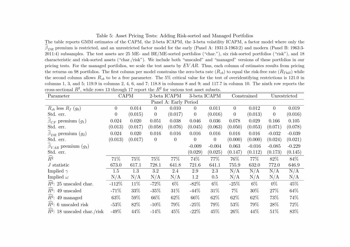
Table 5: Asset Pricing Tests: Adding Risk-sorted and Managed PortfoliosThe table reports GMM estimates of the CAPM, the 2-beta ICAPM, the 3-beta volatility ICAPM, a factor model where only theb premium is restricted, and an unrestricted factor model for the early (Panel A: 1931:3-1963:2) and modern (Panel B: 1963:3-2011:4) subsamples. The test assets are 25 ME- and BE/ME-sorted portfolios (“char.”), six risk-sorted portfolios (“risk”), and 18characteristic and risk-sorted assets (“char./risk”). We include both “unscaled” and “managed” versions of these portfolios in ourpricing tests. For the managed portfolios, we scale the test assets by . Thus, each column of estimates results from pricingthe returns on 98 portfolios. The first column per model constrains the zero-beta rate () to equal the risk-free rate () whilethe second column allows to be a free parameter. The 5% critical value for the test of overidentifying restrictions is 121.0 incolumns 1, 3, and 5; 119.9 in columns 2, 4, 6, and 7; 118.8 in columns 8 and 9; and 117.7 in column 10. The ninth row reports thecross-sectional 2, while rows 13 through 17 report the 2 for various test asset subsets.Parameter CAPM 2-beta ICAPM 3-beta ICAPM Constrained Unrestricted

Panel A: Early Period less (0) 0 0.014 0 0.010 0 0.011 0 0.012 0 0.019Std. err. 0 (0.015) 0 (0.017) 0 (0.016) 0 (0.013) 0 (0.016)b premium (1) 0.024 0.020 0.051 0.038 0.046 0.036 0.078 0.029 0.166 0.105Std. err. (0.013) (0.017) (0.058) (0.076) (0.045) (0.063) (0.050) (0.053) (0.071) (0.078)b premium (2) 0.024 0.020 0.016 0.016 0.016 0.016 0.016 0.016 -0.032 -0.039Std. err. (0.013) (0.017) 0 0 0 0 (0.000) (0.000) (0.024) (0.021)b premium (3) -0.009 -0.004 0.063 -0.016 -0.085 -0.229Std. err. (0.029) (0.025) (0.147) (0.112) (0.173) (0.145)c2 71% 75% 75% 77% 74% 77% 76% 77% 82% 84% statistic 673.0 617.1 728.1 641.8 721.6 641.1 755.9 632.0 772.0 646.9Implied 1.5 1.3 3.2 2.4 2.9 2.3 N/A N/A N/A N/AImplied N/A N/A N/A N/A 1.2 0.5 N/A N/A N/A N/Ac2: 25 unscaled char. -112% 11% -72% 6% -82% 6% -25% 6% 0% 45%c2: 49 unscaled -71% 33% -35% 31% -44% 31% 7% 30% 27% 64%c2: 49 managed 63% 59% 66% 62% 66% 62% 62% 62% 73% 74%c2: 6 unscaled risk -53% 82% -10% 79% -25% 79% 53% 79% 28% 72%c2: 18 unscaled char./risk -49% 44% -14% 45% -22% 45% 26% 44% 51% 83%

Parameter CAPM 2-beta ICAPM 3-beta ICAPM Constrained UnrestrictedPanel B: Modern Period

less (0) 0 0.015 0 -0.013 0 0.004 0 -0.007 0 0.002Std. err. 0 (0.010) 0 (0.014) 0 (0.014) 0 (0.016) 0 (0.009)b premium (1) 0.017 0.006 0.063 0.118 0.055 0.055 0.073 0.100 0.104 0.098Std. err. (0.008) (0.013) (0.043) (0.072) (0.002) (0.000) (0.059) (0.038) (0.026) (0.034)b premium (2) 0.017 0.006 0.008 0.008 0.008 0.008 0.008 0.008 0.000 0.000Std. err. (0.008) (0.013) 0 0 0 0 (0.000) (0.000) (0.014) (0.015)b premium (3) -0.086 -0.096 -0.097 -0.094 -0.096 -0.097Std. err. (0.036) (0.059) (0.053) (0.058) (0.048) (0.047)c2 -10% 1% 19% 25% 47% 59% 62% 63% 68% 68% statistic 447.5 408.9 350.5 296.6 450.7 407.0 386.4 331.8 295.6 294.4Implied 2.2 0.7 8.1 15.3 7.1 7.2 N/A N/A N/A N/AImplied N/A N/A N/A N/A 22.5 24.9 N/A N/A N/A N/Ac2: 25 unscaled char. -58% -7% 26% 47% -52% 28% 39% 44% 56% 56%c2: 49 unscaled -31% -8% 17% 35% 16% 53% 58% 61% 71% 71%c2: 49 managed -2% 2% 16% 16% 63% 61% 62% 63% 65% 65%c2: 6 unscaled risk -24% -50% -9% 17% -31% 49% 52% 44% 51% 50%c2: 18 unscaled char./risk -32% -17% 4% 22% 48% 62% 65% 67% 78% 78%

54

1926 1936 1946 1956 1966 1976 1986 1996 20060

0.02

0.04

0.06

0.08

0.1

0.12

Varia

nce

Year

Real ized VarianceExpected Variance

Figure 1: This figure plots quarterly observations of realized within-quarter daily returnvariance over the sample period 1926:2-2011:4 and the expected variance implied by themodel estimated in Table 1 Panel A.

55

1926 1936 1946 1956 1966 1976 1986 1996 2006­1

­0.5

0

0.5

1

Smoo

thed

 st. 

devs

.

Year

Smoothed Ncf

1926 1936 1946 1956 1966 1976 1986 1996 2006­1

­0.5

0

0.5

1

Smoo

thed

 st. 

devs

.

Year

Smoothed ­Ndr

1926 1936 1946 1956 1966 1976 1986 1996 2006­1

­0.5

0

0.5

1

Smoo

thed

 st. 

devs

.

Year

Smoothed Nv

Figure 2: This figure plots normalized cash-flow news, the negative of normalized discount-rate news, and normalized variance news. The series are smoothed with a trailingexponentially-weighted moving average where the decay parameter is set to 0.08 per quarter,and the smoothed news series is generated asMAt(N) = 0.08Nt+(1−0.08)MAt−1(N). Thisdecay parameter implies a half-life of six years. The sample period is 1926:2-2011:4.

56

1930 1940 1950 1960 1970 1980 1990 2000­4

­2

0

2

4

6

Sta

ndar

d D

evia

tions

Y ear

10­y r LHRVARlagged DEFlagged PE

1930 1940 1950 1960 1970 1980 1990 20000

0.02

0.04

0.06

0.08

0.1

10­y

r LH

RV

AR

Y ear

10­y r LHRVARForecasted Value

Figure 3: We measure long-horizon realized variance (LHRV AR) as the annualized dis-

counted sum of within-quarter daily return variance, LHRV ARh =4∗Σhj=1ρj−1RV ARt+j

Σhj=1ρj−1 . Each

panel of this figure plots quarterly observations of ten-year realized variance, LHRV AR40,over the sample period 1930:1-2001:1. In Panel A, in addition to LHRV AR40, we also plotlagged PE and DEF . In Panel B, in addition to LHRV AR40, we also plot the fitted valuefrom a regression forecasting LHRV AR40 with DEFO, defined as DEF orthogonalized todemeaned PE. The appendix reports the WLS estimates of this forecasting regression.

57

Figure 4: Each diagram plots sample against predicted average excess returns. Test assetsin the top row are the 25 ME- and BE/ME-sorted portfolios and in the bottom row, bothunscaled (black) and scaled by EV AR (red) versions of the 25 ME- and BE/ME-sortedportfolios (asterisks), six risk-sorted portfolios (circles), and 18 characteristic- and risk-sortedportfolios (crosses). Predicted values are from Table 4 (top row) and Table 5 (bottom row)for 1963:3-2011:4. From left to right, the models tested are the Sharpe/Lintner CAPM, theBlack CAPM, the three-factor ICAPM with the zero-beta rate constrained to the risk-freeerate, and the three-factor ICAPM with a free zero-beta rate.

58

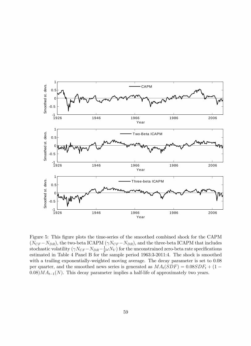
1926 1946 1966 1986 2006­1

­0.5

0

0.5

1

Smoo

thed

 st. 

devs

.

Year

CAPM

1926 1946 1966 1986 2006­1

­0.5

0

0.5

1

Smoo

thed

 st. 

devs

.

Year

Two­Beta ICAPM

1926 1946 1966 1986 2006­1

­0.5

0

0.5

1

Smoo

thed

 st. 

devs

.

Year

Three­beta ICAPM

Figure 5: This figure plots the time-series of the smoothed combined shock for the CAPM(NCF−NDR), the two-beta ICAPM (γNCF−NDR), and the three-beta ICAPM that includesstochastic volatility (γNCF−NDR− 1

2ωNV ) for the unconstrained zero-beta rate specifications

estimated in Table 4 Panel B for the sample period 1963:3-2011:4. The shock is smoothedwith a trailing exponentially-weighted moving average. The decay parameter is set to 0.08per quarter, and the smoothed news series is generated as MAt(SDF ) = 0.08SDFt + (1 −0.08)MAt−1(N). This decay parameter implies a half-life of approximately two years.

59