Interseismic strain accumulation measured by GPSin the seismic gap between Constitución and Concepción in Chile

J.C. Ruegg 1, A. Rudloff 2, C. Vigny 2, R. Madariaga 2,  J.B. Dechabalier 1, J. Campos 3, E. Kausel 3, S. Barrientos 3,  D. Dimitrov 4

1Institut de Physique du Globe (IPGP), Paris, France2Laboratoire de Géologie, Ecole Normale Supérieure (ENS), CNRS, Paris, France3Departamento de Geofísica (DGF), Universidad de Chile, Santiago, Chile4Bulgarian Academy of Sciences, Sofia, Bulgaria

Abstract

The  Concepción­Constitución area [35­37°S] in South Central Chile is very likely a mature 

seismic gap,  since no subduction large earthquake has  occurred there since 1835.   Three 

campaigns of Global Positioning System (GPS) measurements were carried out in this area in 

1996, 1999 and 2002. We observed a network of about 40 sites, including two East­West 

transects ranging from the coastal area to the Argentina border and one North­South profile 

along  the coast.  Our measurements are consistent  with  the Nazca/South America relative 

angular velocity (55. 9°N, 95.2°W, 0.610 °/ Ma) discussed  by Vigny et al., 2007 (this issue) 

which predicts a convergence of   68 mm/yr oriented 79°N at the Chilean trench near 36°S. 

With respect to stable South America, horizontal velocities decrease from 45 mm/yr on the 

coast to 10 mm/yr in the Cordillera. Vertical velocities exhibit a coherent pattern that permits 

us  to constrain  lithospheric  flexure.  Horizontal velocities have formal uncertainties  in  the 

range of 1­2 mm/yr and vertical velocities around 3 to 5 mm/yr. Surface deformation in this 

area   of   South   Central   Chile   is   consistent   with   a   fully   coupled   elastic   loading   on   the 

subduction interface at depth. The best fit to our data is obtained with a dip of 16° +/­ 3°, a 

locking depth of 55 +/­ 5 km and a dislocation corresponding to 68 mm/yr oriented N79°. 

However in the Northern area of our network the fit is improved locally by using a lower dip 

1

1

2

34

567

8

9

10

11

12

13

14

15

16

17

18

19

20

21

22

23

24

25

26

27

28

1

around 13°. Finally a convergence motion of about 68 mm/yr represents  more than 10 m of 

displacement accumulated since the last big interplate subduction event in this area almost 

200 years ago (1835 earthquake described by Darwin). Therefore, in a worst case scenario, 

the area already has a potential for an earthquake of magnitude as large as 8 to 8.5, should it 

happen in the near future.

Introduction

The coastal ranges of Chile are among the most seismically active zones in the world.  On 

average, one major earthquake of magnitude 8 has occurred every 10 years in historical times, 

and most of the individual segments of the coastal ranges have been the site of at least one 

magnitude 8 during the last 130 years [Lomnitz, 1971, Kelleher, 1973, Nishenko, 1985]. One 

exception is  the South­Central Chile region, between 35°S and 37°S, which experienced its 

last largest subduction earthquake on 20 February 1835 [Darwin,  1851] with an estimated 

magnitude   close   to   8.5   [Lomnitz,  1971,   Beck   et   al.,  1998]   (Figure   1).   This   area   lies 

immediately to   the north of  the rupture zone associated  to   the great  1960 earthquake,  of 

magnitude 9.5 [Plafker and Savage,  1970, Cifuentes,  1989] and south of the ruptures zones 

corresponding with the 1928 Talca earthquake [Beck et al.,  1998]   and the 1906 and 1985 

Valparaiso   earthquakes   [Barrientos,   1995].  Part   of   the   region  was   affected  by   the  1939 

Chillán earthquake (magnitude 7.9).  Recent studies demonstrated that this event was not a 

typical  subduction earthquake,  but  was  a  slab­pull  event  due  to   the  release of   tensionnal 

stresses within the downgoing slab [Campos and Kausel,  1990, Beck et al,  1998].  Further 

North, the Talca earthquake of December 1, 1928, was interpreted as a shallow dipping thrust 

event,   [Lomnitz,  1971,   Beck   et   al.,  1998].   Despite   the   uncertainties   that   remain   on   the 

importance of   the 1928 and 1939 earthquakes and  their  impact  on the seismic cycle,   the 

region from 35°S ­37°S is a likely spot for a major subduction earthquake in the coming 

decades. In any case, it is the longest standing gap in Chile, the better known Northern Chile 

gap was affected by large earthquakes in 1868 and 1877 [Lomnitz, 1971, Kelleher, 1973].

2

29

30

31

32

33

34

35

36

37

38

39

40

41

42

43

44

45

46

47

48

49

50

51

52

53

54

55

2

The area located immediately south of the city of Concepción between 37°S and 38°S is 

particularly interesting. The Arauco peninsula is an elevated terrace with respect to the mean 

coastal line. It shows evidences of both quaternary and contemporary uplift.  Darwin [1851] 

reported 3 m of uplift at Santa Maria Island due to the 1835 earthquake. On the other hand, 

this area constitutes the limit between the rupture zones of the 1835 and 1960 earthquakes. As 

such, it might play an important role in the segmentation of the subducting slab. This tectonic 

situation is similar to that of the Mejillones Peninsula which seems to have acted as a limit to 

southward propagation for the 1877 large earthquake in Northern Chile, and to northward 

propagation during the 1995 Antofagasta earthquake [Armijo and Thiele, 1990; Ruegg et al.,  

1996]. 

The seismicity of the region remained largely unkown and imprecise because of the lack of a 

dense seismic network until a  seismic field experiment that was carried out in 1996. The 

results of this experiment reveal the distribution of the current seismicity, focal mechanism 

solutions, and geometry of the subduction [Campos et al., 2001]. 

What is the potential for a future earthquake? How is the current plate motion accommodated 

by crustal strain in this area?  In order to study the current deformation in this region, a GPS 

network was installed in 1996, densified in 1999 with nine new points between the Andes 

mountains   and   the   Arauco   peninsula,   and   finally   resurveyed   entirely   in   2002.   A   first 

estimation of the interseismic velocities in this area was done using the first two campaigns of 

1996 and 1999 [Ruegg et al., 2002]. We report here on the GPS measurements carried out in 

1996, 1999 and 2002, and the interseismic velocities at 36 points sampling the upper plate 

deformation. 

GPS measurements and data analysis

The GPS experiments began in 1996 with the installation of geodetic monuments at thirty 

three sites distributed in 3 profiles and five other scattered points covering the so­called South 

3

56

57

58

59

60

61

62

63

64

65

66

67

68

69

70

71

72

73

74

75

76

77

78

79

80

81

3

Central Chile seismic gap between Concepción to the South and Constitución to the North. 

The Northern transect,  oriented 110°N, includes 8 sites between the Pacific coast and the 

Chile­Argentina border (CO1, CT2,CT3,CT4 COLB, CT6,CT7, CT8) (Figure 1). A coastal 

profile includes 11 sites between PTU north of the city of Constitución city and Concepción 

in the South. A southern profile, roughly oriented W­E was initiated between the Arauco 

peninsula, south of Concepción (2 sites, RMN, LTA and 4 sites between the foothills of the 

Andes and the Chile­Argentina border MRC, MIR, CLP, LLA). Five additional points were 

located   in   the   Central   Valley   area   (BAT,   PUN,   QLA,   NIN,   CHL).     During   the   first 

measurement   campaign   in  December  1996  we  used  9  Ashtech  Z12  and  3  Trimble  SSE 

receivers and type 2 antennas. Each site was surveyed 20­30 hours in average for 2­3 days of 

measurement.

Eight new sites were installed during the March 1999 measurement campaign on the southern 

part  of   the  1996 network   in  order   to   complete   the   southern  profile  between   the  Arauco 

peninsula and the foothills of the Andes (LLI,RAQ,CAP,PUL,LAJ,SLT,SGE) (Figure 1). We 

used 7 Ashtech Z12 equipped with choke­ring antennas. At the same time, 13 points of  the 

1996 network were measured again, providing a first estimation of the interseismic velocity 

field (Ruegg et al., 2002). 

Most of the sites were equipped with brass benchmarks sealed in bedrock outcrops, but the 

measurements were done using tripods and optical tribrachs which enable centering with only 

sub­centimeter accuracy. However, most of the sites were equipped with 3 auxiliary points 

allowing a better permanency. During all campaigns, three points (QLA, PUN, CO6) were 

measured continuously in 24­hour sessions. Other sites were measured for 12 to 24 hours per 

day over 2 to 4 days.  Finally almost the entire network was resurveyed in March 2002 except 

for a few missing points. The current solution gives velocities at 36 sites determined over the 

6 years period. For the GPS data analysis we reduce it in 24­hour sessions to daily estimates 

of   station   positions   using   the   GAMIT   software   [King   and   Bock,   2000],   choosing   the 

ionosphere­free combination, and fixing the ambiguities to integer values. We use precise 

4

82

83

84

85

86

87

88

89

90

91

92

93

94

95

96

97

98

99

100

101

102

103

104

105

106

107

108

4

orbits from the International GPS Service for Geodynamics (IGS) [Beutler et al., 1993]. We 

also   use   IGS   Tables   to   describe   the   phase   centers   of   the   antennae.   We   estimate   one 

tropospheric vertical delay parameter per station every 3 hours. The horizontal components of 

the calculated relative position vectors (Table 1) are accurate to within a few millimetres for 

pairs of stations less than 300 km apart, as measured by the root mean square (RMS) scatter 

about the mean (the so­called baseline repeatability). Daily solutions were recalculated for the 

three epochs including tracking data from a selection of permanent stations (11 for the 2002 

experiment)   in South America,  some of  them belonging to  the International GPS Service 

(IGS) [Neilan, 1995]. Two stations are close to the deformation area, 7 more span the South­

American craton in Brazil, Guyana and Argentina, and the remaining 2 sample the Nazca 

plate.

   In the second step, we combine the daily solutions using the GLOBK software [Herring et  

al., 1990] in a “regional stabilization” approach. We combine daily solutions using Helmert­

like transformations to estimate translation, rotation, scale and Earth orientation parameters 

(polar motion and UT1 rotation). This “stabilization” procedure defines a reference frame by 

minimizing, in the least­square sense, the departure from the prior values determined in the 

International   Terrestrial   Reference   Frame   (ITRF)   2000   [Altamimi   et   al.,   2002].   This 

procedure, described in more details in Vigny et al., 2007 (this issue), estimates the positions 

and velocities for a set of 10 well­determined stations in and around our study area. The 

misfit to these “stabilization” stations is 2.8 mm in position and 1.6 mm/yr in velocity.

Velocity field

This procedure leads to horizontal velocities with respect to ITRF2000 (Table 2). Here we 

present our results both in the ITRF2000 reference frame, and relative to the South­American 

plate by using the angular velocity of this plate (25.4°S, 124.6°W, 0.11°/Myr) given by the 

Nuvel­1A model [Demets et al.,  1994]. Our data set is consistent with that of Vigny et al. 

5

109

110

111

112

113

114

115

116

117

118

119

120

121

122

123

124

125

126

127

128

129

130

131

132

133

134

5

(2007).  First of all, far field stations spanning the South American craton show that the later 

is not affected by any significant internal deformation and that its present day angular velocity 

does not differ significantly from the Nuvel­1A estimate. Second, stations on the Nazca plate 

(EISL   and  GALA)   are   also   consistent   with   their   reduced   Nazca/South  America   angular 

velocity, which predicts 68 mm/yr of convergence oriented 79°N on the trench at the latitude 

of our network.

South Central Chile velocities 

Figure 2 depicts the velocity field with respect to the stable South America reference frame. 

Observed velocities decrease rapidly from the Pacific coast to the Chile Argentina border, 200 

km inland. Coastal stations move inland with velocities close to 35­40 mm/yr while Andean 

stations move with a velocity closer to 10­20 mm/yr. Accordingly, velocity directions rotate 

from their initial strike of 70°N +/­ 1° along the coast (LLI, UCO, CO6, PTU), to 75°N +/­ 

2°in the central valley (SLT, CHL, QLA, CT4), and almost purely East trending in the Andes 

(LLA and CT8).

Because it is the longest profile and because it starts closer to the trench, the southern profile 

between the Arauco peninsula and the Andes is particularly interesting. The nearest point to 

the trench (LLI) show a velocity of 45 ± 2 mm/yr, while the last point in the Andes (LLA), 

presents a velocity of 15 ± 0.5 mm/yr (Figure 3). This implies an accumulation of 30 mm/yr 

over this 200 km long distance, or an integrated strain rate of 1.5 10­6 per year. 

The northern profile between Constitución and the Andes shows slightly less compression: 37 

± 2 mm/yr at CO2 or CO4 and 10 +/­ 0.6 mm/yr at Laguna Maule (CT8) on the top of Andes 

near the Chile­Argentina border (Figure 3). Along this northern profile, stations lying at the 

same distance from the trench have a velocity 10­25 % larger than along the southern profile 

(Figure   3).   Accordingly,   northern   transect   stations   show   a   different   crustal   strain   than 

southern stations: weaker in the first half (100­200 km from the trench) and stronger in the 

6

135

136

137

138

139

140

141

142

143

144

145

146

147

148

149

150

151

152

153

154

155

156

157

158

159

160

6

second half in the foothills of the Andes (200­300 km from trench) (Figure 3). These patterns 

are consistent with the accumulation of elastic strain in the upper plate due to locking on the 

subduction interface with latitude­dependent dip angle (see elastic modelling section).

Although less precisely determined, the vertical velocities exhibit a coherent pattern which, 

like the horizontal ones, is consistent with what is expected from standard elastic modelling. 

Vertical velocities of the coastal stations are negative (indicating subsidence) when those of 

the   Central   Valley   are   positive   (indicating   uplift)   and   those   of   the   Andean   range   are 

essentially near zero (Figure 4a). This is particularly true around the Arauco peninsula where 

distance to the trench is lower than 100 km, and where vertical velocities are negative and less 

than ­10 mm/yr, accordingly with the modelled curve (Figure 4b).

Elastic modeling 

     To model the upper plate deformation during the interseismic stage, we make the usual 

assumption that the interface between the Nazca and South American plates is locked down to 

to a certain depth (the locking depth or coupling depth), while the deeper part is slipping 

continuously  at   the  relative  plate  velocities.  This  defines   the  “seismically  coupled zone”, 

portion of the upper plate interface which might be the site of a future major thrust earthquake 

in the BioBío and Maule regions of Chile.  We model this deformation using a simple back­

slip assumption (Savage, 1983) for which the inter­seismic accumulation correspond exactly 

to the released co­seismic deformation (with reversed sign), and we use Okada's elastic model 

to relate the surface deformation to the dislocation buried at depth [Okada, 1985]. We define 

the geometry of the fault plane model by considering the distribution of earthquakes (Campos 

et al., 2001) and the geometry of the slab as given by Cahill and Isacks (1992). The fault 

plane model is simply defined by 9 parameters: 3 for the location of the of the fault’s center, 

azimuth (strike), dip,   width along the dip and length of the fault plane,   and for the slip 

dislocation vector, the slip modulus and the rake angle.  A strike angle of about N19°E is 

chosen, in agreement with the average direction of both the trench axis and the coast line 

7

161

162

163

164

165

166

167

168

169

170

171

172

173

174

175

176

177

178

179

180

181

182

183

184

185

186

7

between 33°S and 38°S.   A dip angle of 20° is taken for our first trial model but our final 

model uses a dip of 16°.  The updip limit of our fault plane is taken to be at the trench, at a 

depth of 6 km. The centre of the fault model is taken at the average latitude of the observed 

sites (37 °S) and the length of the model extends for a distance of 1000 km along the coast to 

avoid edge effects.  We used the parameters defining the convergence at the trench, 68 mm/yr 

in the direction 79°N, to define the slip vector of the model and the corresponding rake (here ­ 

59° for a back slip model). In summary we fixed 7 parameters and left only two free, the dip 

and the width of the locked plane, to adjust the observed velocities. 

The best fit to our data is obtained with a fault plane of 16° +/­ 3° dip, and a locking depth of 

56 km +/­ 5 km  located a distance of 180 km eastwards from the trench. The fact that the 

imposed dislocation  matches  exactly   the  convergence   rate  of   the  plate   indicates   that   the 

interface is fully locked, or in other words that the coupling between the two plates is 100%. 

This result is in agreement with those of Khazaradze and Klotz (2003) who find a similar 

locking depth and full coupling (100%). 

If this model parameters fit very well (residuals < 2 mm/yr) the southern part (< 36.5°S) of 

our network, residuals are larger (range 4­7 mm/yr) in the northern part for latitude bellow 

35.5°S, the later being particularly true in the neighbourhood of the Central Valley (Figure 5). 

This worsen fit could be due to either a different dip angle of the subduction interface, a 

variation in the dip with distance from the trench, or a change in the locking depth. Indeed, 

the fit can be improved locally by using a slightly reduced dip angle of 13°, which generates a 

longer   slab before   it   reaches   the depths  at  which   it   starts   to   slip   freely.  The usage  of  a 

shallower and longer slab generates an eastward shift of the deformation gradient, such as the 

one observed in our data (Figure 3). Finally, the pattern of vertical deformations modelled 

using   those   elastic   parameters   inferred   from   horizontal   deformations,   matches   well   the 

observed one (Figure 4b). Despite a high level of dispersion the general trend near the trench 

is well observed and the locations of maximum uplift around 200km from the trench also 

correspond within +/­ 20 km..

8

187

188

189

190

191

192

193

194

195

196

197

198

199

200

201

202

203

204

205

206

207

208

209

210

211

212

213

8

Conclusion

In this paper we complete and extent the finding of preliminary results obtained with only two 

GPS campaigns and a lower number of observed sites (Ruegg et al., 2002). Interseismic velo­

cities (horizontal and vertical components) have been determined at 36 sites (against 13 in 

Ruegg et al., 2002), with better uncertainties (formal uncertainties in the range 1­2 mm/yr and 

vertical velocities around 3 to 5 mm/yr). The velocities on the northern transect vary from 36 

mm/yr at   the coast and 10 mm/yr at   the Chile­Argentina border, with a particularly high 

gradient of velocity from the foothills of the Andes to their top (0.5 10­6 per y at 220­320 km 

from trench). The southern transect exhibits very high geodetic speed in the coastal region of 

Arauco (45  mm/yr) which decrease to 15 mm/yr at the top of Andes which implies a strong 

strain accumulation of 1.5 10­6 per y over the 200 km long distance between the coast and the 

top of the Andes. Vertical velocities are negative at the coast, while those measured in the 

Central Valley have positive values and those on the Andean range are close to zero. 

This deformation pattern is very well explained by the elastic loading of the seismogenic zone 

of the plate interface by continuous slip at depth, using as slip vector the convergence rate 

between the two plates (68 mm/yr at 79°N). Thus, it appears that the plates are fully coupled 

with a locking depth situated at  56 km depth at a distance of 180 km from trench. We do not 

know whether   the  plate   interface  has   slipped  episodically   in   the  past,   or  whether   it   has 

remained fully locked since the last big earthquake 1835. In the worst case scenario, that 

strains have not been relieved at all since 1835,  at a convergence rate of 68 mm/yr more than 

10 m of slip deficit have accumulated since 1835. It is possible that the Northern part of the 

plate   interface  between Constitución and Concepción was affected by  the  earthquakes  of 

1851, 1928 and 1939, but it is unlikely that this was the case near the city of Concepción. We 

would   then   conclude   that   the   southern   part   of   the   Concepción­Constitución   gap   has 

accumulated a slip deficit that is large enough to produce a very large earthquake of about 

Mw = 8.0­8.5. This is of course a worst case scenario that needs to be refined by additional 

work.

9

214

215

216

217

218

219

220

221

222

223

224

225

226

227

228

229

230

231

232

233

234

235

236

237

238

239

240

9

Acknowledgments.  This work is part of a cooperative project between Universidad de Chile, 

Santiago, Institut de Physique du Globe de Paris and Ecole Normale Supérieure, Paris. It was 

initiated by a European Community contract CI1­CT94­0109 and   supported by the French 

Ministère des Affaires Etrangères (comité ECOS) and by CNRS/INSU programs, in particular 

by   ACI   CatNat..   We   are   grateful   to   many   people   who   participated   in   measurement 

campaigns, and particularly our colleagues H. Lyon­Caen, E.Clevede and T.Montfret , as well 

as students from DGF and ENS.

References

Altamimi,   Z.,   P.   Sillard,   and   C.   Boucher   (2002),   ITRF2000:   A   new   release   of   the 

International Terrestrial Reference frame for earth science applications, J. Geophys. Res., 

SA 107 (B10): art. no. 2214.

Angermann,  D.,  J.Klotz,  and C.Reigber,   (1999),  Space geodetic  estimation of   the Nazca­

South America Euler vector, Earth Planet. Sci. Lett. 171, 329­334.

Armijo, R.; Thiele, R. (1990), Active faulting in northern Chile: ramp stacking and lateral 

decoupling along a subduction plate boundary? Earth and Planetary Science Letters, Vol. 

98, p. 40­61.

Barrientos,  S.  E.   (1995),  Dual   seismogenic  behavior:   the  1985 Central  Chile  earthquake. 

Geophys. Res. Lett. 22, 3541−3544 .

Beck, S., S. Barrientos, E. Kausel and M. Reyes (1998), Source characteristics of historic 

earthquakes along the central Chile subduction zone, J. South. American Earth Sci., 11, 

115­129.

Beutler, G., J. Kouba, and T. Springer (1993), Combining the orbits of the IGS processing 

centers, in proceedings of IGS annalysis center workshop, edited by J. Kuba, 20­56.

Cahill, T and B. Isacks (1992), Seismicity and shape of the subducted Nazca plate, Jour.  

Geophys. Res. 97, 17503­17529.1

241

242

243

244

245

246

247

248

249

250

251

252

253

254

255

256

257

258

259

260

261

262

263

264

265

26610

Campos J. and E. Kausel (1990), The large 1939 Intraplate earthquake of Soutern Chile, Seis. 

Res. Lett., 61.

Campos, J.,  D. Hatzfeld, R. Madariaga, G. López, E. Kausel, A. Zollo, G. Iannacone, R. 

Fromm, S. Barrientos, et H. Lyon­Caen (2002),  A Seismological study of the 1835 

Seismic gap in South Central Chile. Phys. Earth Planet. Int., 132, 177­195.

Cifuentes, I.L, The 1960  Chilean  earthquake, J. Geophys. Res., 94, 665­680, 1989.

Darwin, C. , Geological observations on coral reefs, volcanic islands and on South America, 

768 pp., Londres, Smith, Elder and Co., 1851.

DeMets, C., et al. (1994), Effect of the recent revisions to the geomagnetic reversal time scale 

on estimates of current plate motions, Geophys. Res. Lett., 21, 2191­2194.

Herring,  T.  A.,  et   al.  (1990),  Geodesy  by   radio  astronomy:    The  application  of  Kalman 

filtering to very long baseline interferometry, J. Geophys. Res., 95, 12,561­512,581.

Kelleher, J. (1972) Rupture zones of large South American earthquakes and some predictions, 

J. Geophys.Res. 77, 2087­2103.

Khazaradze, G., and J. Klotz (2003), Short and long­term effects of GPS measured crustal 

deformation rates along the South­Central Andes. J. of Geophys. Res., 108, n°B4, 1­13

King, R. W.,  and Y. Bock (2000) Documentation for  the GAMIT GPS software analysis 

version 9.9, Mass. Inst. of Technol., Cambridge.

Larson, K.,  J.T. Freymuller, and S. Philipsen (1997), Global consistent rigid plate velocities 

from GPS, J. Geophys. Res., 102,  9961­9981.

Lomnitz C., Grandes terremotos y tsunamis en Chile durante el periodo 1535­1955, Geofis. 

Panamericana, 1, 151­178, 1971.

Neilan, R. (1995), The evolution of the IGS global network, current status and future aspects, 

in IGS annual report, edited by J.F. Zumberge et al., JPL Publ., 95­18, 25­34.

1

267

268

269

270

271

272

273

274

275

276

277

278

279

280

281

282

283

284

285

286

287

288

289

290

11

Nishenko, R. (1985), Seismic potential for large and great intraplate earthquakes along the 

Chilean and Southern Peruvian margins of South America: a quantitative reappraisal.,  J.  

Geophys. Res., 90, 3589­3615.

Okada, Y. (1985), Surface deformation due to shear and tensile faults in a half­space,  Bull.  

Seism. Soc. Am., 75, 1135–1154.

Plafker, G. and J.C. Savage (1970), Mechanism of the Chilean earthquake of May 21 and 22, 

1960, Geol. Soc. Am. Bull., 81, 1001­1030.

Ruegg  J.C.,   J.  Campos,  R.  Armijo,  S.  Barrientos,  P.  Briole,  R.  Thiele,  M.  Arancibia,   J. 

Canuta, T. Duquesnoy, M. Chang, D. Lazo, H. Lyon­Caen, L. Ortlieb, J.C. Rossignol and 

L. Serrurier (1996), The Mw=8.1 Antofagasta earthquake of July 30, 1995 : First results 

from teleseismic and geodetic data, Geophysical Res. Letters, vol.23, no 9, 917­920.

Ruegg J.C., J. Campos, R. Madariaga, E. Kausel, J.B. DeChabalier , R. Armijo, D. Dimitrov, 

I. Georgiev, S. Barrientos (2002), Interseismic strain accumulation in south central Chile 

from   GPS   measurements,   1996­1999,  Geophys.   Res.   Lett.,   29,   no   11, 

10.1029/2001GL013438.

Savage J.C. (1983) A dislocation model of strain accumulation and release at a subduction 

zone, J. Geophys. Res. 88 pp. 4948­4996. 

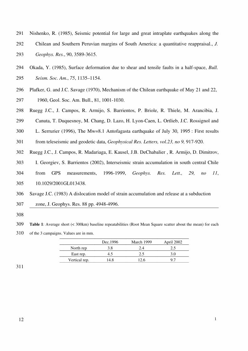
Table 1: Average short (< 300km) baseline repeatabilities (Root Mean Square scatter about the mean) for each 

of the 3 campaigns. Values are in mm.

Dec.1996 March 1999 April 2002North rep 3.8 2.4 2.5East rep. 4.5 2.5 3.0

Vertical rep. 14.8 12.6 9.7

1

291

292

293

294

295

296

297

298

299

300

301

302

303

304

305

306

307

308

309

310

311

12

Table 2: Site positions and velocities, in ITRF2000 and relative to South­America plate. Latitude and longitude 

are in decimal degrees. All velocities and velocity uncertainties are in mm/yr.

Site Position Velocity/IRTF2000 Velocity / SOAM UncertaintiesLongitude Latitude Vlon Vlat Vlon Vlat   s_lon   s_la

t  corr,

BAT ­71.962 ­35.307 32.56 19.62 33.21 9.24 0.48 0.21 0.105CAP ­73.272 ­37.245 34.47 27.41 34.74 17.15 2.35 1.02 0.125CHL ­72.205 ­36.639 26.65 18.89 27.11 8.53 0.99 0.35 0.038CLM ­72.812 ­36.236 33.08 23.02 33.53 12.72 0.95 0.31 ­0.025CLP ­71.625 ­37.336 16.77 11.50 17.21 1.09 0.51 0.26 0.103CO1 ­72.415 ­35.318 36.41 21.55 37.01 11.21 0.86 0.27 ­0.012CO2 ­72.491 ­35.412 34.65 22.97 35.23 12.64 1.06 0.35 0.101CO4 ­72.626 ­35.586 34.70 23.97 35.25 13.65 0.81 0.30 0.108CO6 ­72.606 ­35.828 34.32 23.24 34.84 12.92 0.35 0.15 0.084CO7 ­72.639 ­35.843 35.48 23.13 36.00 12.81 0.96 0.33 0.220CO8 ­72.744 ­35.949 35.46 23.61 35.95 13.30 1.10 0.37 0.270COLB ­71.347 ­35.677 27.21 15.83 27.88 5.39 0.32 0.14 0.071CT2 ­72.255 ­35.464 34.76 20.56 35.36 10.20 0.95 0.32 0.020CT3 ­72.086 ­35.558 33.04 20.26 33.65 9.89 0.75 0.29 0.091CT4 ­71.777 ­35.616 30.08 17.46 30.71 7.06 0.70 0.48 ­0.031CT6 ­71.069 ­35.709 22.49 17.56 23.19 7.09 0.45 0.19 0.001CT7 ­70.834 ­35.815 17.86 13.48 18.57 2.99 0.59 0.22 ­0.039CT8 ­70.399 ­35.991 9.84 11.34 10.58 0.81 0.58 0.29 0.166GUA ­72.333 ­37.346 22.92 16.56 23.28 6.21 2.12 1.35 0.401LAJ ­72.697 ­37.255 25.86 20.55 26.19 10.24 0.68 0.31 0.075LLA ­71.344 ­37.369 14.79 10.95 15.26 0.51 0.54 0.27 0.110LLI ­73.569 ­37.192 42.29 24.92 42.54 14.69 1.61 0.72 0.219LTA ­73.142 ­37.059 30.95 23.87 31.26 13.60 1.10 0.38 0.035MIR ­71.75 ­37.330 16.54 12.60 16.97 2.20 0.73 0.32 0.184MRC ­71.955 ­37.411 18.62 14.02 19.01 3.64 0.50 0.24 0.100NIN ­72.437 ­36.410 34.76 15.56 35.23 5.22 0.46 0.20 0.039PTU ­72.269 ­35.172 32.02 22.88 32.66 12.53 0.67 0.26 0.151PUL ­72.942 ­37.285 30.16 21.03 30.46 10.74 0.68 0.31 0.081PUN ­71.957 ­35.750 31.30 19.90 31.90 9.52 0.35 0.16 0.082QLA ­72.125 ­36.085 29.87 18.28 30.41 7.91 0.31 0.14 0.115RAQ ­73.436 ­37.256 36.44 24.51 36.69 14.27 1.75 0.77 0.272SGE ­72.231 ­37.393 23.90 16.81 24.27 6.45 1.47 0.62 0.334SLT ­72.384 ­37.216 27.66 18.28 28.03 7.94 0.69 0.30 0.025UCO ­73.035 ­36.829 33.77 23.05 34.12 12.77 1.42 0.60 0.141DGF ­70.664 ­33.457 22.93 18.36 23.94 7.86 1.66 0.60 0.039

Permatent sitesSANT ­70.669 ­33.150 19.39 16.64 20.44 6.14 0.21 0.10 0.118AREQ ­71.493 ­16.466 14.20 14.89 17.12 4.46 1.33 0.57 0.023BRAZ ­47.878 ­15.947 ­4.32 12.31 ­0.08 0.64 0.41 0.28 0.041EISL ­109.383 ­27.148 66.00 ­7.72 65.27 ­12.70 0.34 0.24 0.080GALA ­90.304 ­0.743 51.76 12.15 56.26 3.99 0.88 0.88 ­0.002

1

312

313

314

13

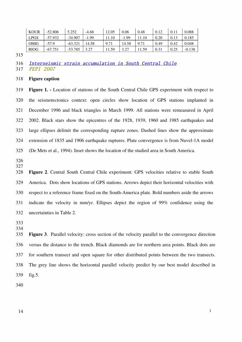
KOUR ­52.806 5.252 ­4.68 12.05 0.06 0.48 0.12 0.11 0.088LPGS ­57.932 ­34.907 ­1.99 11.10 ­1.99 11.10 0.20 0.13 0.185OHIG ­57.9 ­63.321 14.58 9.71 14.58 9.71 0.49 0.42 0.048RIOG ­67.751 ­53.785 3.27 11.59 3.27 11.59 0.31 0.25 ­0.138

Interseismic strain accumulation in S outh C entral Chile PEPI 2007

Figure caption

Figure 1. ­  Location of stations of the South Central Chile GPS experiment with respect to 

the   seismotectonics   context:   open   circles   show   location   of   GPS   stations   implanted   in 

December 1996 and black triangles in March 1999. All stations were remeasured in April 

2002. Black stars show the epicentres of the 1928, 1939, 1960 and 1985 earthquakes and 

large ellipses delimit the corresponding rupture zones. Dashed lines show the approximate 

extension of 1835 and 1906 earthquake ruptures. Plate convergence is from Nuvel­1A model 

(De Mets et al., 1994). Inset shows the location of the studied area in South America. 

Figure 2.  Central South Central Chile experiment: GPS velocities relative to stable South 

America.  Dots show locations of GPS stations. Arrows depict their horizontal velocities with 

respect to a reference frame fixed on the South­America plate. Bold numbers aside the arrows 

indicate   the   velocity   in  mm/yr.   Ellipses   depict   the   region  of   99%  confidence   using   the 

uncertainties in Table 2. 

Figure 3.  Parallel velocity: cross section of the velocity parallel to the convergence direction 

versus the distance to the trench. Black diamonds are for northern area points. Black dots are 

for southern transect and open square for other distributed points between the two transects. 

The grey line shows the horizontal parallel velocity predict by our best model described in 

fig.5.  

1

315

316317

318

319

320

321

322

323

324

325

326327328

329

330

331

332

333334335

336

337

338

339

340

14

Figure 4. Vertical component of the displacement. (a) map of vertical velocities, (b) vertical 

velocities in mm/yr versus the distance to the trench of each station. The grey line shows the 

vertical component of the model described in fig.5.  

Figure 5. Elastic modeling of the upper plate deformation in the South Central Chile gap. 

(a): GPS observations (brown arrows) and model predictions (white arrows) are shown. Inset 

describes the characteristics of the model.   (b):  residual (i.e. observations­model) velocities 

are shown (black arrow). In both boxes, the grey contour line and shaded pattern draw the 

subduction plane buried at depth and the white arrows depict the dislocation applied on this 

plane. 

1

341

342

343

344345346

347

348

349

350

351

15

Figure 1.   ­  Location of  stations  of   the  South Central  Chile  GPS experiment  with  respect   to   the seismotectonics  context: open circles show location of GPS stations implanted in December 1996 and black   triangles in March 1999. All stations were remeasured in April 2002. Black stars show the epicenters of the 1928, 1939, 1960 and 1985 earthquakes and large ellipses delimit the corresponding rupture zones. Dashed lines show the approximate extension of 1835 and 1906 earthquake ruptures. Plate convergence is from Nuvel­1A model (De Mets et al., 1994). Inset shows the location of the studied area in South America. 

1

352353354355356357358359360

16

Figure 2. Central South Central Chile experiment: GPS velocities relative to stable South America. Dots show locations of GPS stations. Arrows depict their horizontal velocities with respect to a reference frame fixed on the South­America plate. Bold numbers aside the arrows indicate the velocity in mm/yr. Ellipses depict the region of 99% confidence using the uncertainties in Table 2. 

1

361362363364365366367

17

Figure  3.     Parallel   velocity:   cross   section  of   the  velocity  parallel   to   the   convergence 

direction versus the distance to the trench. Black diamonds are for northern area points. 

Black dots are for southern transect and open square for other distributed points between 

the two transects. The grey line shows the horizontal parallel velocity predict by our best 

model described in fig.5.  

1

368

369370371

372

373

374

375

376377378379380381

18

Figure 4. Vertical component of the displacement. (a) map of vertical velocities, (b) vertical velocities in mm/yr 

versus the distance to the trench of each station. The grey line shows the vertical component of the model 

described in fig.5.  

1

382383

384

385

386

19

Figure 5. Elastic modeling of the upper plate deformation in the South Central Chile gap. (a):  GPS   observations   (brown   arrows)   and   model   predictions   (white   arrows)   are   shown.   Inset describes the characteristics of the model.  (b): residual (i.e. observations­model) velocities are shown (black arrow). In both boxes,  the grey contour line and shaded pattern draw the subduction plane buried at depth and the white arrows depict the dislocation applied on this plane. 

2

387

388

38939039139239339439539639720

Fig 5   (b):  residual (i.e. observations­model) velocities are shown (black arrow). In both boxes, the grey contour line and shaded pattern draw the subduction plane buried at depth and the white arrows depict the dislocation applied on this plane.

2

398399400401402403

404405406407408

21