international trade and factor mobility: an empirical

International Trade and Factor Mobility:An Empirical Investigation

byLinda S. Goldberg and Michael W. Klein

Abstract

Foreign Direct Investment (FDI) has been growing rapidly, at a pace far exceeding thegrowth in international trade. Thus, a full understanding of the relationship between tradein goods and FDI is important for obtaining a complete picture of the extent and sourcesof international linkages. We investigate whether FDI serves as a complement to trade ora substitute for trade based on the effects identified by the Rybczynski theorem wherebyan increase in a factor of production used intensively in one sector affects production bothin that sector and in other sectors. Using detailed data on bilateral capital and trade flowsbetween the United States and individual Latin American countries, we examine thelinkages between FDI into particular sectors of Latin American economies and the netexports of those and other manufacturing sectors. We find that FDI from the UnitedStates can lead to significant, and varied, shifts in the composition of activity in manyLatin American countries and across many manufacturing industries.

First Draft: October 1997Revised: May 18 1999

Linda S. Goldberg Michael W. KleinFederal Reserve Bank of New York Fletcher School, Tufts University,

and N.B.E.R. and N.B.E.R.

JEL codes: F31, F3, F4

This paper was prepared for the Festschrift in Honor of Robert Mundell. The viewsexpressed in this paper are those of the individual authors and do not necessarily reflectthe position of the Federal Reserve Bank of New York or the Federal Reserve System.We thank Alan Winters for comments on an earlier draft. Jenessa Gunther and KevinCaves provided excellent research assistance. Address correspondences to Linda S.Goldberg, Federal Reserve Bank of NY, Research Department, 33 Liberty St,NY,NY10045. Tel:212-720-2836; fax:212-720-6831; email: [email protected].

1

I. Introduction

It is a notable achievement to develop an economic model that provides a

framework for understanding and analyzing important economic issues of the day. It is an

even more striking achievement to develop an economic model that addresses an issue that

will be of central importance in the future. In the 1950s, a time when cross-border capital

movements were largely stymied by government regulations, Robert Mundell published a

series of papers studying the implications of capital mobility. Today’s central paradigms

for studying events in a world characterized by vast flows of capital across national

boundaries draw on Mundell’s analysis that foresaw such a world. An examination of the

linkages between international capital movements, domestic production and international

trade is especially timely today, given the massive and volatile capital flows to emerging

markets observed through the 1990s.

Mundell studied capital mobility in a variety of frameworks. He is best known for

the Mundell-Fleming model which analyzes the effect of portfolio capital movements on

the efficacy of monetary and fiscal policy. Monetary authorities today are intimately

aware of the central lessons of this model. Less well-known, but increasingly relevant, are

issues considered in Mundell’s work on the implications of physical capital mobility for

international trade. In a world of significant growth of both international direct investment

and international trade, this work raises important considerations for policy-makers who

are concerned with understanding trade and direct investment linkages among countries.

In “International Trade and Factor Mobility” (1957), Mundell demonstrates the

substitutability of international trade and factor mobility. In the context of the Heckscher-

Ohlin-Samuelson model, perfect factor mobility across sectors within an economy

provides a tendency for commodity-price equalization, even in the absence of international

trade in goods. This result complements the Stolper-Samuelson theorem, which

demonstrates the tendency for factor-price equalization as a consequence of goods trade,

even in the absence of international trade in factors. International factor mobility also

serves as a substitute for trade in another sense in the Heckscher-Ohlin-Samuelson (H-O-

S) model, since an increase in the volume of factor movements can decrease the volume of

trade.

2

Subsequent theoretical work has demonstrated that models which diverge from the

standard H-O-S assumptions can result in complementarity, rather than substitutability,

between factor trade and goods trade (Wong 1986). There are a variety of ways this

subsequent work differs from Mundell’s original contribution, including allowances for

differences in technologies across countries (Kemp 1966, Jones 1967, Purvis 1972,

Svensson 1984, and Markusen and Svensson 1985), introduction of production taxes,

monopoly market structure, external economies of scale or factor market distortions

(Markusen 1983) and permitting foreign capital to promote domestic development

(Schmitz and Helmberger 1970). In all of these cases, an increase in international direct

investment may promote greater international trade.

Understanding the relationship between trade in goods and trade in factors is

important for obtaining a complete picture of international linkages. For example, it is

often the case that the amount of international trade undertaken by a country serves as a

proxy for its level of “openness” or, in a bilateral context, as a measure of the international

linkages between two countries. Mundell’s analysis implies that focusing on trade as a

proxy for openness may be misleading when international capital flows are significant.

Empirically, it is important to consider whether this bias is significant and systematic in a

particular direction.

Another key reason for understanding these linkages arises in the aftermath of the

currency and financial crises of the 1990s. If capital inflows to a country are large, but

also can abruptly change course, important real consequences can ensue. In Latin

America, in Asia, or elsewhere, even exogenous reversals in foreign capital availability can

lead to a redistribution of productive factors within a country. The availability of

investment funds and new physical capital can have important consequences for the future

structure of a country’s trade and the welfare of its citizens.

The broad challenge posed by the theoretical and policy arguments can only be

resolved through careful analytical and empirical studies. Recent empirical research in this

area includes work by Collins, O’Rourke and Williamson (1997), who studied the

historical link between labor mobility and trade, and our own work on the response of

exports and imports of selected Latin American and Southeast Asian countries to direct

3

investment from the United States and Japan (Goldberg and Klein 1998). Collins,

O’Rourke and Williamson found little evidence of substitutability between labor

movement and trade. We found some evidence of complementarity between capital flows

and bilateral trade, especially in the Asian region: direct investment from Japan to

Southeast Asian countries significantly increased the bilateral exports and imports of those

countries with Japan. We found no evidence of significant links between capital flows and

bilateral trade, however, between Latin American countries and either Japan or the United

States, or between the United States and Southeast Asian countries.

In this paper we provide a motivating theoretical model, followed by a detailed

empirical study of the effects of direct investment flows on levels of international trade.

We present the first empirical analysis, to our knowledge, of this relationship at a sectoral

level. Specifically, we study how the net exports of specific manufacturing sectors of eight

Latin American countries (Argentina, Brazil, Chile, Colombia, Ecuador, Mexico, Peru,

and Venezuela) respond to direct investment from the United States into those specific

sectors, as well as into other manufacturing and non-manufacturing sectors of their

economies. We demonstrate empirically the varied direction and levels of response of

sectoral trade volumes to direct investment across manufacturing sectors and across

countries.

Based on this detailed empirical evidence, we conclude that the theoretical debate

is justified. In Argentina, where investments into manufacturing industries have been

concentrated in Food-related industries or Chemical industries, the net exports of these

industries have expanded (despite these industries remaining net importers overall),

without significant detriment to other manufacturing industries. In Brazil and Venezuela,

FDI into particular manufacturing industries – flows that have been concentrated in

Chemicals, Machinery and Transportation Equipment – have been associated with

expanded net import positions by these industries. Foreign investment into Wholesale &

Retail Trade worsened the net export positions of manufacturing industries in Mexico and

Columbia (suggesting that this FDI facilitated Latin imports), but improved the net export

positions in Brazilian manufacturing industries. Our detailed examination of the

4

experience of individual industries, using cross-country and time-series data, does not

suggest strong or systematic linkages between sectoral trade and FDI in Latin America.

II. Direct Investment in Sector-Specific Capital and Trade

II A. Overview. To set the stage for our empirical analysis, in this section we review the

main distinctions between general equilibrium models that find that factor mobility and

trade are substitutes, versus those models that find that they are complements. We then

present a simple version of the Rybczynski theorem to highlight the role of sector-specific

capital. Our objective is use the theoretical exposition to motivate our empirical tests for

sectoral trade volumes and foreign direct investment linkages, allowing both for direct

effects on trade of foreign capital inflows into a sector and for spillovers effects from

inflows into other sectors.

In these general equilibrium models, the relative returns to factors and the level of

production and trade are jointly determined. Typically, models differ in their predictions

about the relationship between factor movements and trade volumes because of

differences in assumptions about production, which lead to differences in the relative

returns to factors. Across models, however, the manner in which the change in a factor

endowment affects the production of each good in the economy is similar. The basis of

this relationship is the Rybczynski theorem, which then drives the association between

factor flows and trade volumes.

We illustrate the Rybczynski-based association between capital flows and trade

volumes in the context of two types of models: in the first, countries differ in their

endowments of factors but have identical production technologies (a Heckscher-Ohlin-

Samuelson style model). In the second, production technologies are different in the two

countries (a Ricardian style model). Basic forms of these models include two goods and

two factors -- labor and capital. In this setting, the Rybczynski theorem states that, given

the prices of goods, an inflow of capital leads to an increase in the level of production of

the good which uses capital relatively intensively, and a decrease in the level of production

of the good which uses labor relatively intensively. These changes in production have

direct implications for trade volumes and, in fact, will be the sole source of changes in

5

trade volumes under the assumption of homothetic and identical preferences in each

country.

Mundell studied the relationship between factor flows and trade in a H-O-S model.

He considered a situation where a prohibitively-high tariff on imports shuts off trade and

raises the return to capital in the country where it is the relatively scarce factor. This leads

to a capital inflow to that country and, through the Rybczynski effect, an increase in the

production of the capital-intensive good (which had been the imported good before the

tariff was put in place) and a decrease in the production of the labor-intensive good (which

had been the export). Capital inflows continue until relative factor endowments in the two

countries are identical.

If the tariff were then removed, there would be no trade in goods. The reason is

that the initial basis for trade in this model, autarky differences in relative factor

endowments and the accompanying differences in relative goods prices, has been

eliminated through factor flows. Factor flows can give rise to commodity price

equalization, much as in the standard H-O-S model goods trade gives rise to factor price

equalization. More broadly, in a model of this nature, an increase in the volume of factor

flows causes a decrease in the volume of trade. Factor flows substitute for trade flows.

An alternative result can arise in a Ricardian model in which countries have

different technologies. For example, suppose each of two countries has the same labor

productivity but one country enjoys higher capital productivity. The country with the

higher capital productivity will export the capital-intensive good. When capital is

internationally mobile, it will seek its highest returns and thus flow to the high capital-

productivity country. Through the Rybczynski effect, these capital inflows increase the

production of the capital intensive good (that country’s export) and decrease the

production of the labor intensive good (that country’s import). In this simple example,

factor flows complement trade flows.

II B. A Basic Specific – Factors Model

A basic model provides a context for our empirical exploration of the way in which

foreign direct investment to a particular sector affects the volume of exports and imports

6

of that sector as well as of other sectors. There are two goods, A and B. The factors of

production include domestic and foreign capital used solely in the production of good A,

KA and FA, respectively, domestic and foreign capital used solely in the production of good

B, KB, and FB, respectively, and labor, L. Labor, unlike capital, costlessly shifts from one

sector to another in response to an incipient wage differential. The amount of labor used in

the production of good A is denoted as LA and the amount used in the production of good

B is denoted as LB.

There are two other key assumptions in this partial-equilibrium analysis. First,

domestic and foreign capital are completely sector specific. The assumption that foreign

capital is sector-specific reflects the prevalent view that direct investment typically

involves some active management of an asset. (This treatment contrasts with a view of

portfolio investment as only requiring the bearer to passively hold the asset.) The direct

management of foreign investment requires some sector-specific knowledge that makes an

investor focus on a sector within which she has particular expertise.

The second key assumption is that foreign direct investment is exogenous, an

assumption which makes this a partial-equilibrium exercise. This clearly runs counter to

the standard modeling assumption of perfect capital mobility since it does not allow for

arbitraging rates of return across sectors.1 The implication of this second assumption is

that we do not endogenously determine the equalization of returns to investments across

borders, or the equilibrium volume of international capital flows.2 A general equilibrium

approach could accomplish this goal, but it would likely still give rise to similar qualitative

results as those shown using the simple partial equilibrium setting.

Assume that production functions take the form

( )BBBAAA LFKgBLFKfA ,),( +=+= (1)

1 Recent research questions the assumption of the equalization of rates of return for a variety of types ofcapital. Most relevant in this context is the work of Froot and Stein (1991) who model foreign directinvestment with imperfect capital markets. Empirical results in their paper, as well as in research byKlein and Rosengren (1994), suggest that there is a lack of perfect capital mobility for direct investment.2 Markusen (1995) argues that there is little evidence that direct foreign investment is related todifferences in factor endowments across countries or to differences in the general return to capital.

7

where the partial derivatives with respect to labor, ( )f gL L, , and capital, ( )f gK K, , are

positive. The cross-partial derivatives with respect to labor and capital from either foreign

or domestic sources, ( )f gLK LK, , also are positive. All second partial derivatives,

( )f f g gLL KK LL KK, , , , are negative.

With labor perfectly mobile across sectors and the labor market competitive, the

wage paid to labor in Sector A, w, is the same as the wage paid to labor in Sector B. The

first-order conditions for profit maximization require that firms in each sector hire labor to

the point where the product wage equals the marginal product of labor,

w

pf

w

pg

AL

BL= = (2)

Totally differentiating each of these relationships, and dividing through by the product

wage or the marginal product of labor, we obtain

dw

w

dp

p

f

fdL

f

fdF

dw

w

dp

p

g

gdL

g

gdF

A

A

LL

LA

LK

LA

B

B

LL

LB

LK

LB

− =

+

− =

+

(3)

where dLi represents the change in employment in sector i and dFi represents foreign

direct investment to sector i. Setting dKi equal to zero reflects our assumption of sector-

specific domestic capital and our interest in considering the effects of FDI rather than

changes in domestic capital. 3 Full employment of labor ensures that L L LA B= + , where

L is the total amount of labor in the economy. With a constant labor force4, we have

dL dLA B= − (4)

3 The structure of production given in equation 1 implies that domestic and foreign capital are perfectsubstitutes within a sector.4 We could easily assume a growing labor force, an assumption which would not change our results.

8

Wages are continuously equated across the two sectors, and, therefore, the proportionate

change in wages across sectors is equal. Solving the sets of equations for the change in

labor in each sector yields:

dLf g

ZdF

g f

ZdF

f g

Z

dp

p

dp

p

dLf g

ZdF

f g

ZdF

f g

Z

dp

p

dp

p

ALK L

ALK L

BL L A

A

B

B

BL LK

BLK L

AL L B

B

A

A

=

−

+

−

=

−

+

−

(5)

where ( )Z f g g fLL L LL L= − + > 0.

These equations show that foreign direct investment to Sector A (dFA >0) pulls

labor into that sector, reducing the labor employment in Sector B (dFB >0), all else equal.

The implication is that a collapse of (foreign) capital in a sector leads that sector to

contract employment, leaving labor to flow to the other sector. The marginal products of

labor and the degree of complementarities between labor and capital in production

determine the magnitudes of the worker reallocation.

There are straightforward output implications of these labor and capital

adjustments. From the production functions,

dA f dF f dLK A L A= + (6)

dB g dF g dLK B L B= +

Substituting in the results from above, we obtain

dAf g

Z

dp

p

dp

pf

f g f

ZdF

f g

ZdF

dBg f

Z

dp

p

dp

pg

g g f

ZdF

g f

ZdF

L L A

A

B

BK

LK L LA

L LKB

L L B

B

A

AK

LK L LB

L LKA

= −

+ +

−

= −

+ +

−

2 2

2 2(7)

These equations show that sectoral output is stimulated by an increase in its relative price

or by FDI into that sector; its output is decreased by FDI into the other sector. The basic

intuition is that an inflow of foreign capital into a sector increases sectoral output directly,

9

by providing more capital, and indirectly, by raising the marginal product of its labor and

drawing workers away from the other sector. Overall, investment to one sector increases

production in that sector and decreases production in the other sector, all else equal.

Returning to the issue originally considered by Mundell and others, the implication

of these results is that the effects of FDI on trade volumes depend upon whether a sector

was initially a net exporter or a net importer. Assuming no demand-side effects (as would

be consistent with the assumption of homothetic demand), and that relative price effects

are second order, an increase in production in Sector A causes international trade by that

sector to increase if that sector was initially a net exporter, or to decrease if that sector

was initially a net importer. The converse also holds. In all these cases, direct investment

into a sector should cause an increase in the net exports of that sector and a decrease in

the net exports of other sectors, all else equal.

III. Capital and Trade Flows with Latin America

A. Data. In this section we explore the relationship between trade and FDI using detailed

sectoral data on FDI inflows and trade between the United States and eight Latin

American countries: Argentina, Brazil, Chile, Colombia, Ecuador, Mexico, Peru, and

Venezuela5 (sources: United States Bureau of Economic Analysis Statistics on US Direct

Investment Abroad and the Feenstra NBER Trade Database). The data on FDI span both

manufacturing and non-manufacturing industries; the bilateral trade data spans only the

manufacturing industries. The sample period for which both trade and FDI data are

available is 1972 through 1994. Trade, investment, and US income series are converted

into real dollar values using the United States producer price series. The GDP series for

individual Latin American countries enters in the regressions as millions of real local

currency units.

5 In order to make the sector definitions consistent across the trade and the FDI series, we use themanufacturing decomposition delineated by the FDI numbers, i.e. with a breakdown into Food andKindred Products, Chemicals and Allied Products, Primary and Fabricated Metals, Industrial Machineryand Equipment, Electronic and Other Electric Machinery, Transportation, and Other Manufacturing.Data also are available for FDI into non- manufacturing sectors, which are comprised of Wholesale Trade,Banking, Finance, Services, and Other Industries. These later series are somewhat less complete, sinceobservations are sometimes not disclosed if the scale of specific investments can be traced to individualinvestors from the United States.

10

Chart 1: US FDI by Region*

-11000

-6000

-1000

4000

9000

14000

19000

24000

29000

34000

39000

73 75 77 79 81 83 85 87 89 91 93

Rea

l FD

I, M

illio

ns

of

1990

US

Do

llars

Asia-Pacific

Latin America

Europe

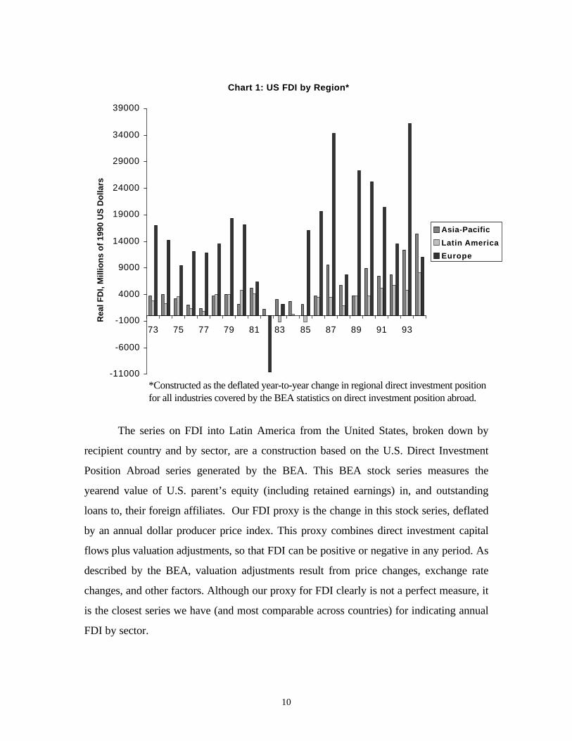
*Constructed as the deflated year-to-year change in regional direct investment positionfor all industries covered by the BEA statistics on direct investment position abroad.

The series on FDI into Latin America from the United States, broken down by

recipient country and by sector, are a construction based on the U.S. Direct Investment

Position Abroad series generated by the BEA. This BEA stock series measures the

yearend value of U.S. parent’s equity (including retained earnings) in, and outstanding

loans to, their foreign affiliates. Our FDI proxy is the change in this stock series, deflated

by an annual dollar producer price index. This proxy combines direct investment capital

flows plus valuation adjustments, so that FDI can be positive or negative in any period. As

described by the BEA, valuation adjustments result from price changes, exchange rate

changes, and other factors. Although our proxy for FDI clearly is not a perfect measure, it

is the closest series we have (and most comparable across countries) for indicating annual

FDI by sector.

11

Chart 2: Annual FDI from the US*

-2000

-1000

0

1000

2000

3000

4000

73 75 77 79 81 83 85 87 89 91 93

Rea

l FD

I, M

illio

ns

of

1990

US

Do

llars

Argentina

Brazil

Mexico

*Source: BEA statistics on US direct investment position abroad. Constructed asthe sum over all manufacturing and nonmanufacturing industries in the sample ofthe the deflated year-to-year change in direct investment position.

Latin American countries have been regular recipients of erratic U.S. outward

investment flows over the past decades. As shown in Chart 1, U.S. FDI flows to various

regions, including Latin America, and the Asia-Pacific area have been growing following a

period of decline and stagnation in the early to mid 1980s. In general, FDI flows to Latin

America account for about 13 percent of US FDI to the three major FDI recipient regions

(Europe, Latin America, and Asia-Pacific). Within Latin America, the main recipient

countries have been Brazil, Mexico, and Argentina, respectively accounting for

approximately 45, 30 and 10 percent of the region's inflows from the United States over

12

the two decades we examine. Chart 2 shows the considerable volatility of these flows

across countries and over time.6

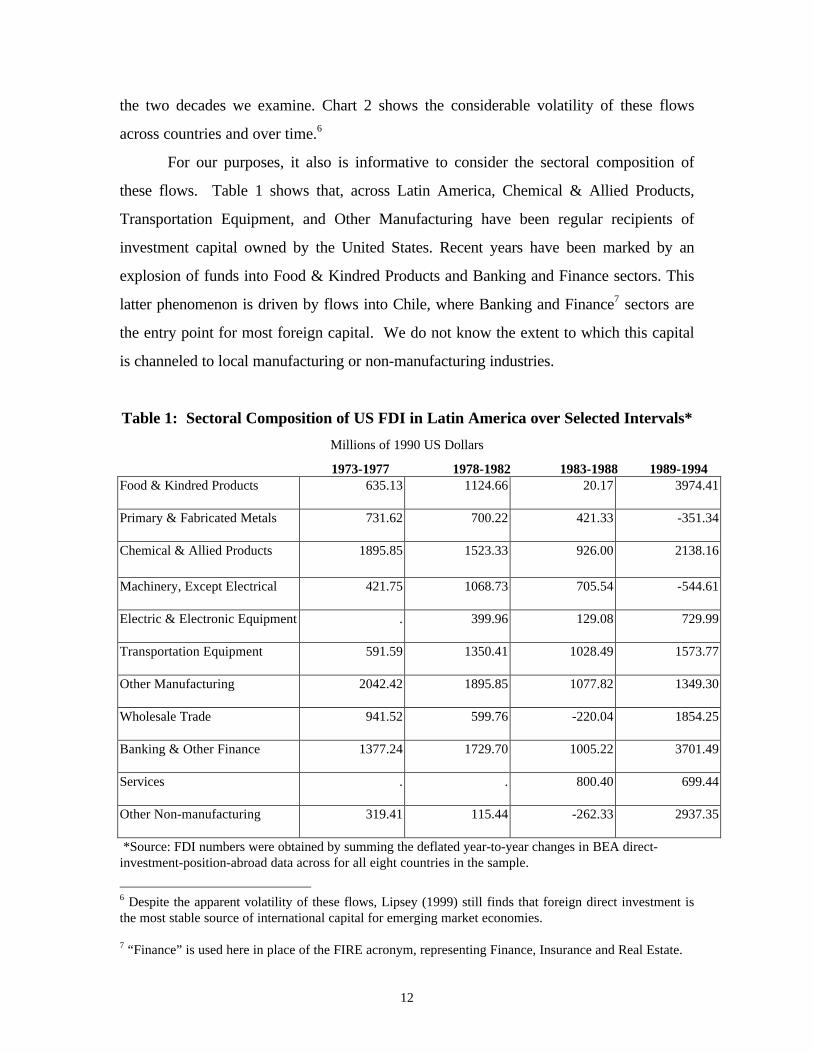
For our purposes, it also is informative to consider the sectoral composition of

these flows. Table 1 shows that, across Latin America, Chemical & Allied Products,

Transportation Equipment, and Other Manufacturing have been regular recipients of

investment capital owned by the United States. Recent years have been marked by an

explosion of funds into Food & Kindred Products and Banking and Finance sectors. This

latter phenomenon is driven by flows into Chile, where Banking and Finance7 sectors are

the entry point for most foreign capital. We do not know the extent to which this capital

is channeled to local manufacturing or non-manufacturing industries.

Table 1: Sectoral Composition of US FDI in Latin America over Selected Intervals*

Millions of 1990 US Dollars

1973-1977 1978-1982 1983-1988 1989-1994Food & Kindred Products 635.13 1124.66 20.17 3974.41

Primary & Fabricated Metals 731.62 700.22 421.33 -351.34

Chemical & Allied Products 1895.85 1523.33 926.00 2138.16

Machinery, Except Electrical 421.75 1068.73 705.54 -544.61

Electric & Electronic Equipment . 399.96 129.08 729.99

Transportation Equipment 591.59 1350.41 1028.49 1573.77

Other Manufacturing 2042.42 1895.85 1077.82 1349.30

Wholesale Trade 941.52 599.76 -220.04 1854.25

Banking & Other Finance 1377.24 1729.70 1005.22 3701.49

Services . . 800.40 699.44

Other Non-manufacturing 319.41 115.44 -262.33 2937.35

*Source: FDI numbers were obtained by summing the deflated year-to-year changes in BEA direct-investment-position-abroad data across for all eight countries in the sample.

6 Despite the apparent volatility of these flows, Lipsey (1999) still finds that foreign direct investment isthe most stable source of international capital for emerging market economies.

7 “Finance” is used here in place of the FIRE acronym, representing Finance, Insurance and Real Estate.

13

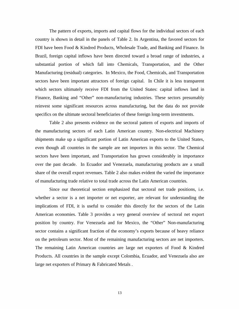
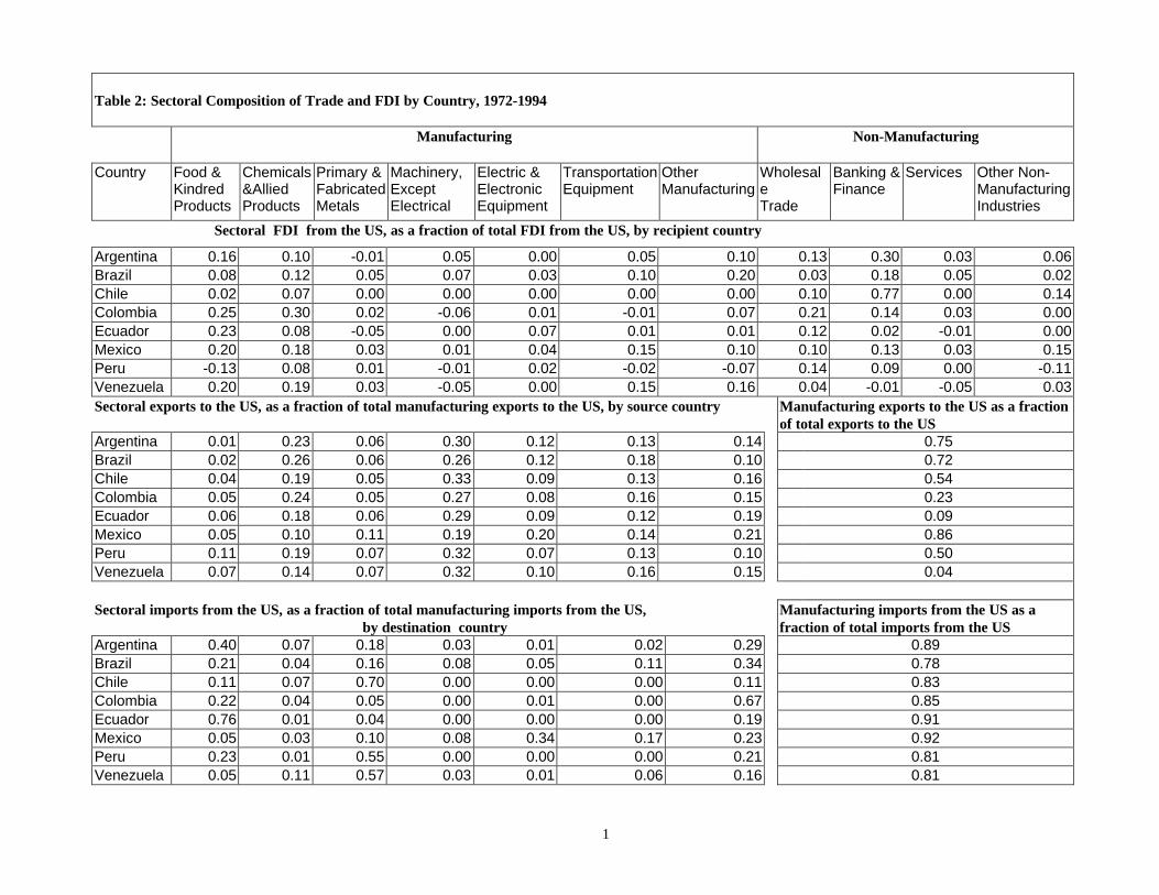
The pattern of exports, imports and capital flows for the individual sectors of each

country is shown in detail in the panels of Table 2. In Argentina, the favored sectors for

FDI have been Food & Kindred Products, Wholesale Trade, and Banking and Finance. In

Brazil, foreign capital inflows have been directed toward a broad range of industries, a

substantial portion of which fall into Chemicals, Transportation, and the Other

Manufacturing (residual) categories. In Mexico, the Food, Chemicals, and Transportation

sectors have been important attractors of foreign capital. In Chile it is less transparent

which sectors ultimately receive FDI from the United States: capital inflows land in

Finance, Banking and “Other” non-manufacturing industries. These sectors presumably

reinvest some significant resources across manufacturing, but the data do not provide

specifics on the ultimate sectoral beneficiaries of these foreign long-term investments.

Table 2 also presents evidence on the sectoral pattern of exports and imports of

the manufacturing sectors of each Latin American country. Non-electrical Machinery

shipments make up a significant portion of Latin American exports to the United States,

even though all countries in the sample are net importers in this sector. The Chemical

sectors have been important, and Transportation has grown considerably in importance

over the past decade. In Ecuador and Venezuela, manufacturing products are a small

share of the overall export revenues. Table 2 also makes evident the varied the importance

of manufacturing trade relative to total trade across the Latin American countries.

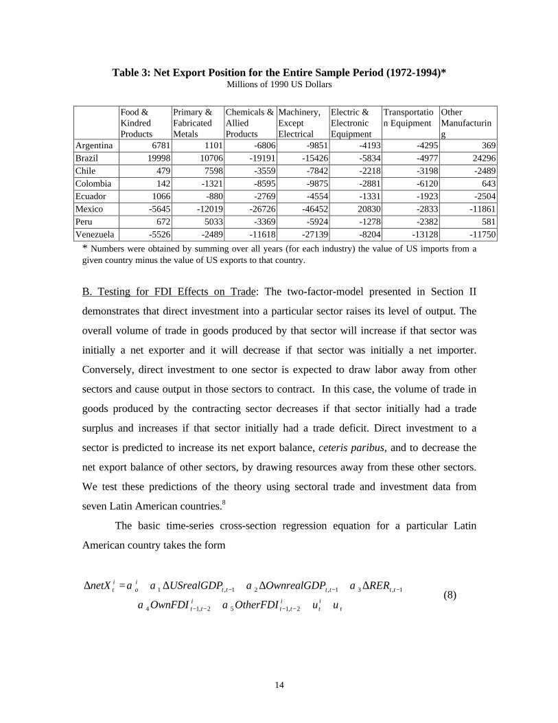
Since our theoretical section emphasized that sectoral net trade positions, i.e.

whether a sector is a net importer or net exporter, are relevant for understanding the

implications of FDI, it is useful to consider this directly for the sectors of the Latin

American economies. Table 3 provides a very general overview of sectoral net export

position by country. For Venezuela and for Mexico, the “Other” Non-manufacturing

sector contains a significant fraction of the economy’s exports because of heavy reliance

on the petroleum sector. Most of the remaining manufacturing sectors are net importers.

The remaining Latin American countries are large net exporters of Food & Kindred

Products. All countries in the sample except Colombia, Ecuador, and Venezuela also are

large net exporters of Primary & Fabricated Metals .

1

Table 2: Sectoral Composition of Trade and FDI by Country, 1972-1994

Manufacturing Non-Manufacturing

Country Food &KindredProducts

Chemicals&AlliedProducts

Primary &FabricatedMetals

Machinery,ExceptElectrical

Electric &ElectronicEquipment

TransportationEquipment

OtherManufacturing

WholesaleTrade

Banking &Finance

Services Other Non-ManufacturingIndustries

Sectoral FDI from the US, as a fraction of total FDI from the US, by recipient country

Argentina 0.16 0.10 -0.01 0.05 0.00 0.05 0.10 0.13 0.30 0.03 0.06Brazil 0.08 0.12 0.05 0.07 0.03 0.10 0.20 0.03 0.18 0.05 0.02Chile 0.02 0.07 0.00 0.00 0.00 0.00 0.00 0.10 0.77 0.00 0.14Colombia 0.25 0.30 0.02 -0.06 0.01 -0.01 0.07 0.21 0.14 0.03 0.00Ecuador 0.23 0.08 -0.05 0.00 0.07 0.01 0.01 0.12 0.02 -0.01 0.00Mexico 0.20 0.18 0.03 0.01 0.04 0.15 0.10 0.10 0.13 0.03 0.15Peru -0.13 0.08 0.01 -0.01 0.02 -0.02 -0.07 0.14 0.09 0.00 -0.11Venezuela 0.20 0.19 0.03 -0.05 0.00 0.15 0.16 0.04 -0.01 -0.05 0.03Sectoral exports to the US, as a fraction of total manufacturing exports to the US, by source country Manufacturing exports to the US as a fraction

of total exports to the USArgentina 0.01 0.23 0.06 0.30 0.12 0.13 0.14 0.75Brazil 0.02 0.26 0.06 0.26 0.12 0.18 0.10 0.72Chile 0.04 0.19 0.05 0.33 0.09 0.13 0.16 0.54Colombia 0.05 0.24 0.05 0.27 0.08 0.16 0.15 0.23Ecuador 0.06 0.18 0.06 0.29 0.09 0.12 0.19 0.09Mexico 0.05 0.10 0.11 0.19 0.20 0.14 0.21 0.86Peru 0.11 0.19 0.07 0.32 0.07 0.13 0.10 0.50Venezuela 0.07 0.14 0.07 0.32 0.10 0.16 0.15 0.04

Sectoral imports from the US, as a fraction of total manufacturing imports from the US,by destination country

Manufacturing imports from the US as afraction of total imports from the US

Argentina 0.40 0.07 0.18 0.03 0.01 0.02 0.29 0.89Brazil 0.21 0.04 0.16 0.08 0.05 0.11 0.34 0.78Chile 0.11 0.07 0.70 0.00 0.00 0.00 0.11 0.83Colombia 0.22 0.04 0.05 0.00 0.01 0.00 0.67 0.85Ecuador 0.76 0.01 0.04 0.00 0.00 0.00 0.19 0.91Mexico 0.05 0.03 0.10 0.08 0.34 0.17 0.23 0.92Peru 0.23 0.01 0.55 0.00 0.00 0.00 0.21 0.81Venezuela 0.05 0.11 0.57 0.03 0.01 0.06 0.16 0.81

14

Table 3: Net Export Position for the Entire Sample Period (1972-1994)*Millions of 1990 US Dollars

Food &KindredProducts


Chemicals &AlliedProducts



Transportation Equipment

OtherManufacturing

Argentina 6781 1101 -6806 -9851 -4193 -4295 369Brazil 19998 10706 -19191 -15426 -5834 -4977 24296Chile 479 7598 -3559 -7842 -2218 -3198 -2489Colombia 142 -1321 -8595 -9875 -2881 -6120 643Ecuador 1066 -880 -2769 -4554 -1331 -1923 -2504Mexico -5645 -12019 -26726 -46452 20830 -2833 -11861Peru 672 5033 -3369 -5924 -1278 -2382 581Venezuela -5526 -2489 -11618 -27139 -8204 -13128 -11750

* Numbers were obtained by summing over all years (for each industry) the value of US imports from agiven country minus the value of US exports to that country.

B. Testing for FDI Effects on Trade: The two-factor-model presented in Section II

demonstrates that direct investment into a particular sector raises its level of output. The

overall volume of trade in goods produced by that sector will increase if that sector was

initially a net exporter and it will decrease if that sector was initially a net importer.

Conversely, direct investment to one sector is expected to draw labor away from other

sectors and cause output in those sectors to contract. In this case, the volume of trade in

goods produced by the contracting sector decreases if that sector initially had a trade

surplus and increases if that sector initially had a trade deficit. Direct investment to a

sector is predicted to increase its net export balance, ceteris paribus, and to decrease the

net export balance of other sectors, by drawing resources away from these other sectors.

We test these predictions of the theory using sectoral trade and investment data from

seven Latin American countries.8

The basic time-series cross-section regression equation for a particular Latin

American country takes the form

tit

itt

itt

ttttttio

it

uOtherFDIOwnFDI

REROwnrealGDPUSrealGDPnetX

υαα

αααα

++++

∆+∆+∆+=∆

−−−−

−−−

2,152,14

1,31,21,1(8)

15

where )netXit represents the change in net exports of sector i. )USrealGDP represents

the change in real GDP of the United States; )OwnrealGDP represents the change in the

real GDP of the Latin American country; )RER represents the change in the real exchange

rate of that country (with a positive value representing a dollar appreciation); OwnFDIi

represents the direct investment flow from the United States into sector i; OtherFDI i

represents the direct investment flow to all manufacturing sectors other than sector i, i0α is

a fixed-effects dummy variable on levels of net exports for manufacturing sector i; and

subscripts on these variables refer to time periods.

The subscript t,t-1 reflects the inclusion in the regressions of both a current and a

lagged term, while the subscript t-1,t-2 reflects the inclusion of both a one-period and a

two-period lag. Thus the coefficients αi represent two coefficients, one on the

contemporaneous variable and one on the lagged variable or, in the case of the FDI

variables, one on the variable lagged one period and one on the variable lagged two

periods. The model presented above suggests that the sum of coefficients represented by

the coefficient "4 is positive while the sum of the coefficients represented by the

coefficient "5 is negative. Standard trade models suggest that the sum of coefficients

represented by each of the coefficient "1, "2 and "3 are positive.9

The results from the regression analysis can be combined with information on net

trade flows to address the question of whether direct investment promotes or diminishes

trade. A positive and significant coefficient on the change in own-sector direct

investment 4α indicates that direct investment promotes trade if the country’s bilateral

trade balance with the United States is negative. This case, corresponding to Mundell’s

analysis, is one in which direct investment decreases overall trade by reducing exports

from the United States to the particular country (assuming that the negative overall trade

statistic does not mask a shift from a long-standing negative position to a larger positive

position which has only occurred for a few years in the sample period). Conversely, the

8 Because of missing data, we exclude Ecuador from this part of our empirical analysis.9 The change in the real exchange rate, the change in domestic income and the change in United Statesincome are aggregate regressors in that they have the same value across all sectors in any particular year.Aggregate regressors of this type preclude the use of time dummy variables and require the adjustment ofthe standard errors, as shown by Kloeck (1981).

16

combination of a positive and significant value of 4α or with a positive trade balance for a

country indicates that direct investment to that country promotes trade by expanding an

already-existing trade surplus. This corresponds to the situation in the Ricardian model

discussed above. A negative and significant value of the coefficient on other-sector direct

investment, 5α , combined with a national bilateral trade deficit with the United States

suggests that direct investment promotes the volume of trade, all else equal, by increasing

trade flows from the United States. Conversely, when a country has a bilateral trade

surplus with the United States, direct investment to one sector which diminishes net

exports of other sectors serves to reduce the overall volume of trade, all else equal.

The error term in the regression equation (8) consists of an error specific to the

particular industry for the particular year, itu , and an error common to all industries in the

country for that year, tv . The presence of the common error term, tv , can typically be

addressed using a fixed-effects dummy variable or, equivalently, subtracting the year-

specific mean value from all the variables in the regression. In this case, however, we have

regressors common to all industries in any particular year, such as the change in the real

exchange rate, the change in domestic income and the change in United States income.

Thus we cannot subtract out the year-specific mean value since these aggregate regressors

are common across all cross-sectional units. Instead, we use an iterative procedure which

estimates the variance of tv and then adjusts the variance-covariance matrix in an

appropriate manner (see Kloeck 1981 for a discussion of this problem and its resolution).

17

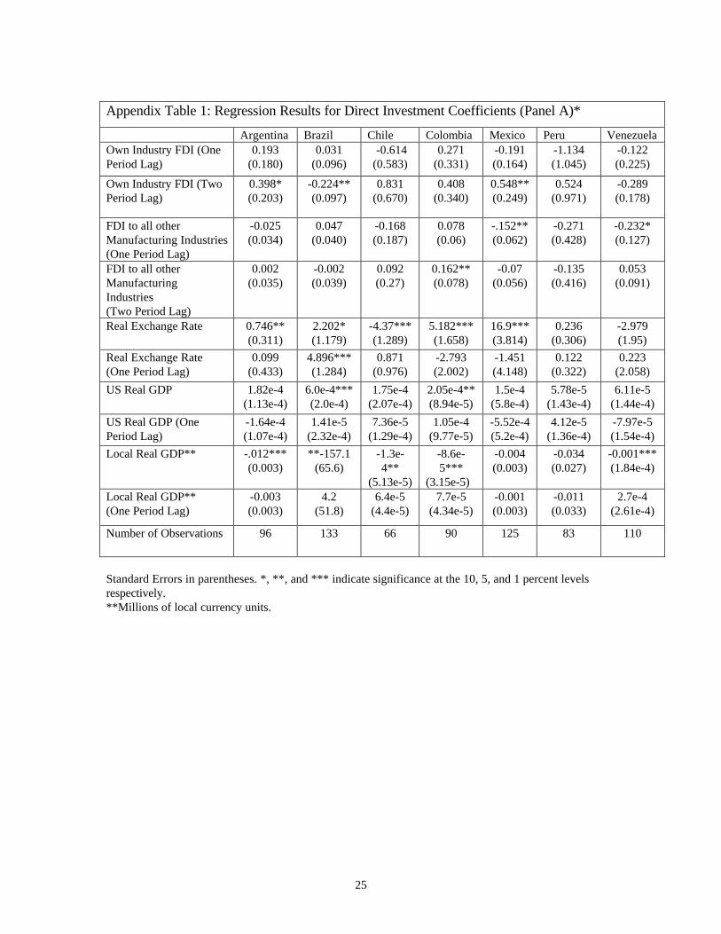
C. Empirical Results: Summary results for regressions using the specification in equation

(8) are presented in the two panels of Table 4. Each of these panels represents sets of

regressions, where the sets are differentiated by the amount of information included in the

other-sector FDI variable. In regressions summarized in Panel A, each country’s

regression contains terms for own industry FDI and for FDI elsewhere in

manufacturing.10

Table 4: Regression Results for Direct Investment Coefficients: Summed Two-Period Effects

Argentina Brazil Chile Colombia Mexico Peru Venezuela

Panel A

Own Industry FDI 0.591**(0.272)

-0.193(0.138)

0.217(0.876)

0.679(0.485)

0.358(0.299)

-0.611(1.56)

-0.151(0.309)

FDI to othermanufacturingIndustries

-0.023(0.044)

0.045(0.046)

-0.076(0.28)

0.24**(0.113)

-.222**(0.095)

-0.406(0.709)

-0.179(0.153)

Number ofObservations

96 133 66 90 125 83 110

Panel B

Own Industry FDI 0.533(0.363)

-0.242*(0.138)

0.546(1.083)

-0.072(0.778)

0.519(0.4)

-0.859(1.657)

-0.716*(0.378)


0.01(0.057)

0.027(0.041)

-0.225(0.412)

0.129(0.228)

0.29(0.232)

-0.326(0.758)

-0.487**(0.242)

FDI to Wholesaleand Retail Trade

-0.424(0.332)

.803***(0.234)

0.178(0.933)

-13.36**(5.538)

-1.49**(0.716)

0.592(1.515)

3.438(2.138)

FDI to Banking,Finance,Insurance, andReal Estate

0.153(0.256)

-0.043(0.071)

0.068(0.178)

0.934(0.937)

-1.151(0.818)

-0.131(1.468)

1.259*(0.666)


76 133 66 69 110 83 91

Standard Errors in parentheses. *, **, and *** indicate significance at the 10, 5, and 1 percent levels respectively.

10 Appendix Table1 provides estimates of the individual regression coefficients that form the basis of thenumbers reported in the body of the text and in Table 4, Panel A. Appendix Table 2 feeds in Panel B.

18

Panel A results suggest that a significant role is played by own-sector FDI in

promoting net exports in Argentina. Own-sector direct investment promotes net exports

in Mexico with a one-year lag, as shown in the complete results presented in Appendix

Table 1. By summing across the rows for Argentina and Mexico in Table 3, we observe

that both countries have a bilateral trade deficit with the United States with respect to

manufactured goods. Thus for these countries, which represent two of the three largest

United States trading partners in Latin America, there is evidence that own-sector direct

investment has the marginal effect of reducing the volume of bilateral trade in a way

consistent with Mundell’s analysis.

The results in Panel A also suggest that other-sector direct investment tends to

reduce net exports in Mexico and increase net exports in Columbia. This mitigates, but

does not reverse, the conclusion that direct investment to Mexico tends to reduce the

volume of trade since the sum of the coefficients on own-sector direct investment, 0.358,

is greater, in absolute value, of the sum of the coefficients on other-sector direct

investment, -0.222. For Colombia, the marginal effect of direct investment is to promote

exports and, therefore, reduce the volume of bilateral trade in manufacturing goods since

both the own-sector and other-sector coefficients are positive.

In Panel B, we allow for direct investment into non-manufacturing sectors to also

affect the output and, therefore, the trade of manufacturing sectors. There are two

possible channels through which these implications may arise. The first channel is that

associated with labor reallocation across sectors, as emphasized in the model presented

above. The second channel recognizes the role of the output of one sector as an input to

the production of other sectors. In this way, direct investment to, for instance, the

financial sector may serve to increase output in manufacturing sectors, as the expanded

finance sector serves the needs of the manufacturing sectors. Likewise, expansion of the

wholesale trade sector may enable manufacturing sectors to expand output for domestic

sales, or it may lead to expanded opportunities for imports. Given the tendency toward

manufacturing sector trade deficits with the United States, a positive coefficient on non-

manufacturing direct investment implies that this type of direct investment causes a decline

in the volume of bilateral trade with the United States while a negative coefficient means

19

that this type of direct investment serves to increase the volume of bilateral trade, all else

equal.

Table 4, Panel B, presents summed two-year net export effects derived from

regressions which include both own-sector and other-manufacturing-sector direct

investment, plus two other sectoral direct investment measures: direct investment in the

Finance, Banking and Real Estate sectors and direct investment in the Wholesale and

Retail Trade sector. These results show that foreign direct investment into the Banking,

Finance and Real Estate sectors, as well as to the Wholesale and Retail Trade sector, have

a significant effect on cross-sectional sectoral trade in a number of countries although the

direction of this effect differs across countries. Direct investment to the Wholesale and

Retail Trade sector has a positive and significant effect on trade by manufacturing sectors

in Brazil and, with a one-period lag only, in Venezuela. Conversely, direct investment to

this sector has a negative and significant effect on trade by manufacturing sectors in

Colombia and Mexico. The effect of direct investment into the Banking, Finance and Real

Estate sectors on trade by manufacturing sectors is significant for Argentina, Mexico and

Venezuela. In Argentina and Mexico, the initial effect is to promote trade while the effect

after one year is to diminish trade. In Venezuela, direct investment to the Finance,

Banking and Real Estate sectors also significantly increases trade at the ninety- percent

level of confidence, with a significant coefficient on the two-year lag at the ninety-five

percent level of confidence.

A comparison of the results in Panel A and Panel B shows that the inclusion of

direct investment from these non-manufacturing sectors also affects the pattern of

significance on the own-sector and other-manufacturing sector direct investment variables.

But some of these differences arise due to differences in the samples available when

including the non-manufacturing direct investment measures. The sample sizes for the

results in Panel B are smaller than those in Panel A. Using the restricted samples

employed in Panel B, but running regressions of the form presented in Panel A,

coefficients on direct investment variables which are reported as significant in Panel A for

Argentina, Mexico (on own-sector direct investment) and Venezuela are no longer

significant.

20

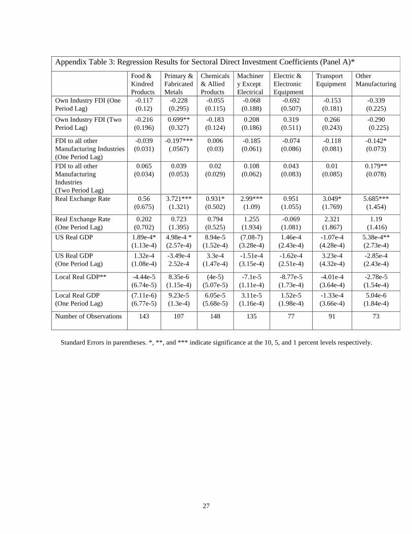
Our second and final group of regressions were run on data grouped by industry,

instead of by country. The regression specification employed is analogous to the one used

in the country regressions, and incorporates appropriate modifications. Specifically, since

the industry regressions include as the left-hand-side variable the net export data for one

industry and several countries, the industry dummies are discarded in favor of country

dummies. These regressions do not require the type of correction to the variance-

covariance matrix discussed above since regressors such as the real exchange rate and

income are not common to all cross-sectional units in a particular year.

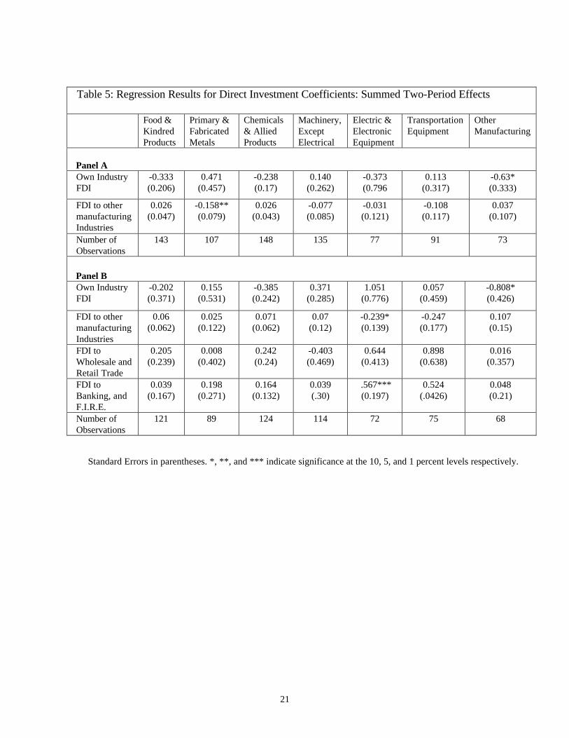
Table 5 displays regression results for the cumulative effects of lagged independent

variables. The results for own industry FDI are less illuminating for these regressions than

those obtained in the country runs; own industry FDI affects trade significantly only in the

case of the “Other Manufacturing” (residual) category, where FDI flows stifle net exports

after one year while stimulating them after two, the cumulative effect being a decrease in

net exports.

Stronger evidence is provided for the role of FDI into other industries in drawing

resources away from Primary and Fabricated Metals. In addition, FDI to industries other

than Electric & Electronic Equipment sector had a significant negative effect on trade in

that industry after one year; the same coefficient was negative but insignificant after two

years, causing the cumulative effect of both coefficients to be insignificant. The regression

results for the Electric & Electronic Equipment sector also provides evidence that banking

and other types of financial FDI inflows stimulate net exports.

21

Table 5: Regression Results for Direct Investment Coefficients: Summed Two-Period Effects



Chemicals& AlliedProducts




OtherManufacturing

Panel AOwn IndustryFDI

-0.333(0.206)

0.471(0.457)

-0.238(0.17)

0.140(0.262)

-0.373(0.796

0.113(0.317)

-0.63*(0.333)


0.026(0.047)

-0.158**(0.079)

0.026(0.043)

-0.077(0.085)

-0.031(0.121)

-0.108(0.117)

0.037(0.107)


143 107 148 135 77 91 73

Panel BOwn IndustryFDI

-0.202(0.371)

0.155(0.531)

-0.385(0.242)

0.371(0.285)

1.051(0.776)

0.057(0.459)

-0.808*(0.426)


0.06(0.062)

0.025(0.122)

0.071(0.062)

0.07(0.12)

-0.239*(0.139)

-0.247(0.177)

0.107(0.15)

FDI toWholesale andRetail Trade

0.205(0.239)

0.008(0.402)

0.242(0.24)

-0.403(0.469)

0.644(0.413)

0.898(0.638)

0.016(0.357)

FDI toBanking, andF.I.R.E.

0.039(0.167)

0.198(0.271)

0.164(0.132)

0.039(.30)

.567***(0.197)

0.524(.0426)

0.048(0.21)


121 89 124 114 72 75 68


22

4. Concluding Remarks

The increasing importance of foreign direct investment in the world economy calls

for theoretical and empirical investigations into the manner in which FDI affects the

linkages among countries. A central question concerning FDI is whether it increases or

decreases the volume of trade. Mundell’s early contribution showed a channel through

which investment substitutes for trade, while later theoretical research presents cases

where trade and investment may serve as substitutes or complements.

Our theoretical model highlights some basic aspects of the different channels

through which foreign direct investment can alter the sectoral composition of capital and

labor in an economy. We provide the results of a detailed examination of the linkages

between FDI into particular sectors of Latin American economies and the net exports of

those and other manufacturing sectors. Our analysis indicates that some FDI tends to

expand manufacturing trade, while other FDI clearly reduces the volumes of

manufacturing trade. In Latin American countries, FDI from the United States can lead to

significant, and varied shifts in the composition of activity in many countries across many

manufacturing sectors.

Given the mixed pattern linkages, it is reasonable to ask whether the Latin

American results are expected to generalize to other partnering relationships among

countries around the world. We conjecture that bilateral sectoral investment and trade

flows-- other than those between the United States and Latin America-- may reveal

stronger relationships than the mixed picture presented here. For example, in our earlier

work (Goldberg and Klein 1998) we present evidence of relatively strong and significant

effects of overall bilateral direct investment from Japan on the overall bilateral trade of

Southeast Asian countries. The weakest results in that earlier paper were for the effects of

United States direct investment on the trade of Latin American countries. Those results

did not use data disaggregated by sectors and, unfortunately, data availability precluded us

from studying the effects of sectoral direct investment from Japan. While the Latin

American results that we have presented do not provide strong evidence that capital flows

systematically and generally expand on contract trade flows, the experiences of other

important regions around the world could also provide important lessons.

23

References

Collins, William J., Kevin H. O’Rourke and Jeffrey G. Williamson, “Were Trade andFactor Mobility Substitutes in History?” N.B.E.R. Working Paper Number 6059, June1997.

Froot, Kenneth and Jeremy Stein, “Exchange Rates and Foreign Direct Investment: AnImperfect Capital Markets Approach,” Quarterly Journal of Economics, vol. 106, 1991,pp. 1191-1217.

Goldberg, Linda S. and Michael W. Klein, 1998. “Foreign Direct Investment, Trade andReal Exchange Rate Linkages in Developing Countries,” in Reuven Glick ed. ManagingCapital Flows and Exchange Rates: Lessons from the Pacific Basin (CambridgeUniversity Press).

Jones, Ronald W., “International Capital Movements and the Theory of Tariffs andTrade,” Quarterly Journal of Economics, volume 81, February 1967, pp. 1-38.

Kemp, Murray C., “The Gain from International Trade and Investment: A Neo-Heckscher-Ohlin Approach,” American Economic Review, volume 61, September 1966,pp. 788-809.

Klein, Michael W. and Eric Rosengren, “The Real Exchange Rate and Foreign DirectInvestment in the United States: Relative Wealth vs. Relative Wage Effects,” Journal ofInternational Economics, vol. 36, 1994, pp. 373-389.

Kloeke, Teun, 1981. “OLS Estimation in a Model Where A Microvariable is Explained byAggregates and Contemporaneous Disturbances are Equicorrelated,” Econometrica vol49 no 1 (January) pp. 205-207.

Lipsey, Robert E., 1999. “The Role of Foreign Direct Investment in International CapitalFlows.” NBER working paper 7094 (April).

Markusen, James R., “Factor Movements and Commodity Trade as Complements,”Journal of International Economics, volume 13, 1983, pp. 341-356.

Markusen, James R., “The Boundaries of Multinational Enterprises and the Theory ofInternational Trade” Journal of Economic Perspectives Spring 1995 vol. 9 no. 2, pp. 169-189.

Markusen, James R. and Lars E.O. Svensson, “Trade in Goods and Factors withInternational Differences in Technology,” International Economic Review, volume 26,1985, pp. 175-192.

24

Mundell, Robert, “International Trade and Factor Mobility,” American Economic Review,volume 47, June 1957, pp. 321-335.

Purvis, Douglas D., “Technology, Trade and Factor Mobility,” Economic Journal, volume82, 1972, pp. 991-999.

Schmitz, Andrew and Peter Helmberger, “Factor Mobility and International Trade: TheCase of Complementarity,” American Economic Review, volume 60, 1970, pp. 761-767.

Svensson, Lars E.O., “Factor Trade and Goods Trade,” Journal of InternationalEconomics, volume 16, 1984, pp. 365-378.

Wong, Kar-yiu, “Are International Trade and Factor Mobility Substitutes?” Journal ofInternational Economics, volume 21, no. 1/2, August 1986, pp. 25-44.

25

Appendix Table 1: Regression Results for Direct Investment Coefficients (Panel A)*

Argentina Brazil Chile Colombia Mexico Peru VenezuelaOwn Industry FDI (OnePeriod Lag)

0.193(0.180)

0.031(0.096)

-0.614(0.583)

0.271(0.331)

-0.191(0.164)

-1.134(1.045)

-0.122(0.225)

Own Industry FDI (TwoPeriod Lag)

0.398*(0.203)

-0.224**(0.097)

0.831(0.670)

0.408(0.340)

0.548**(0.249)

0.524(0.971)

-0.289(0.178)

FDI to all otherManufacturing Industries(One Period Lag)

-0.025(0.034)

0.047(0.040)

-0.168(0.187)

0.078(0.06)

-.152**(0.062)

-0.271(0.428)

-0.232*(0.127)

FDI to all otherManufacturingIndustries(Two Period Lag)

0.002(0.035)

-0.002(0.039)

0.092(0.27)

0.162**(0.078)

-0.07(0.056)

-0.135(0.416)

0.053(0.091)

Real Exchange Rate 0.746**(0.311)

2.202*(1.179)

-4.37***(1.289)

5.182***(1.658)

16.9***(3.814)

0.236(0.306)

-2.979(1.95)

Real Exchange Rate(One Period Lag)

0.099(0.433)

4.896***(1.284)

0.871(0.976)

-2.793(2.002)

-1.451(4.148)

0.122(0.322)

0.223(2.058)

US Real GDP 1.82e-4(1.13e-4)

6.0e-4***(2.0e-4)

1.75e-4(2.07e-4)

2.05e-4**(8.94e-5)

1.5e-4(5.8e-4)

5.78e-5(1.43e-4)

6.11e-5(1.44e-4)

US Real GDP (OnePeriod Lag)

-1.64e-4(1.07e-4)

1.41e-5(2.32e-4)

7.36e-5(1.29e-4)

1.05e-4(9.77e-5)

-5.52e-4(5.2e-4)

4.12e-5(1.36e-4)

-7.97e-5(1.54e-4)

Local Real GDP** -.012***(0.003)

**-157.1(65.6)

-1.3e-4**

(5.13e-5)

-8.6e-5***

(3.15e-5)

-0.004(0.003)

-0.034(0.027)

-0.001***(1.84e-4)

Local Real GDP**(One Period Lag)

-0.003(0.003)

4.2(51.8)

6.4e-5(4.4e-5)

7.7e-5(4.34e-5)

-0.001(0.003)

-0.011(0.033)

2.7e-4(2.61e-4)

Number of Observations 96 133 66 90 125 83 110

Standard Errors in parentheses. *, **, and *** indicate significance at the 10, 5, and 1 percent levelsrespectively.**Millions of local currency units.

26

Appendix Table 2: Regression Results for Direct Investment Coefficients (Panel B)*

Argentina Brazil Chile Colombia Mexico Peru VenezuelaOwn Industry FDI (OnePeriod Lag)

0.079(0.251)

-0.001(0.095)

-1.241*(0.738)

0.29(0.49)

-0.183(0.196)

-1.217(1.092)

-0.351(0.259)


0.455*(0.274)

-0.242**(0.096)

1.997**(0.864)

-0.14(0.571)

0.702**(0.316)

0.358(1.055)

-0.365(0.287)

FDI to all otherManufacturingIndustries(One Period Lag)

-0.001(0.034)

0.02(0.035)

-0.717**(0.325)

0.061(0.103)

-0.162(0.115)

-0.269(0.465)

-0.244(0.163)


0.012(0.049)

0.007(0.032)

0.597*(0.336)

0.133(0.171)

0.453***(0.171)

-0.057(0.457)

-0.243(0.248)

FDI to Wholesale TradeIndustries (One Period Lag)

-0.278(0.216)

0.387***(0.132)

-0.36(0.458)

-8.76**(3.988)

-0.105(0.414)

0.437(1.247)

2.301***(0.764)

FDI to Wholesale TradeIndustries(Two Period Lag)

-0.147(0.172)

0.415***(0.132)

0.803(0.642)

-3.25*(1.868)

-1.343***(0.474)

0.156(1.054)

1.148(1.632)

FDI to Banking, F.I.R.E. (One Period Lag)

0.972**(0.396)

0.05(0.06)

-0.104(0.169)

0.696(0.442)

0.617***(0.225)

-0.415(0.942)

-0.46(0.581)

FDI to Banking, F.I.R.E.(Two Period Lag)

-0.819**(0.410)

-0.934(0.061)

0.152(0.104)

-0.016(0.648)

-1.768*(0.937)

0.284(1.157)

1.719**(0.792)

Real Exchange Rate -1.368(0.928)

2.776***(0.952)

-7.1***(1.545)

8.452***(1.882)

20.118***(4.66)

0.191(0.339)

7.716(5.092)


1.111(0.897)

4.003***(1.027)

0.575(0.888)

-31.50**(12.693)

-5.602(5.976)

0.109(0.354)

7.511(6.889)

US Real GDP 3.29e-4**(1.29e-4)

0.001***(1.94e-4)

5.4e-4***(2.1e-4)

-3.84e-5(2.04e-4)

7.61e-5(5.65e-4)

8.65e-5(1.6e-4)

8.64e-4(6.44e-4)


-4.6e-4***

(1.21e-4)

4.31e-4*(2.34e-4)

1.41-4(1.37-4)

-4.43e-4(3.72e-4)

7.76e-6(5.18e-4)

4.19e-5(1.7e-4)

-1.03-e4(3.93e-4)

Local Real GDP** -0.028***(0.007)

-274.***

(65.3)

-2.5e-4***

(6.28e-5)

-2.48e-5(3.67e-5)

-0.005*(0.003)

-0.032(0.036)

-0.002***(5.85e-4)

Local Real GDP(One Period Lag)

-0.003(0.005)

-81.3(50.6)

1.34e-4**(5.52e-5)

3.11e-4**(1.35e-4)

-0.004(0.003)

-0.019(0.044)

-5.04e-4(9.94e-4)



27

Appendix Table 3: Regression Results for Sectoral Direct Investment Coefficients (Panel A)*




Machinery ExceptElectrical


TransportEquipment

OtherManufacturing

Own Industry FDI (OnePeriod Lag)

-0.117(0.12)

-0.228(0.295)

-0.055(0.115)

-0.068(0.188)

-0.692(0.507)

-0.153(0.181)

-0.339(0.225)


-0.216(0.196)

0.699**(0.327)

-0.183(0.124)

0.208(0.186)

0.319(0.511)

0.266(0.243)

-0.290 (0.225)

FDI to all otherManufacturing Industries(One Period Lag)

-0.039(0.031)

-0.197***(.0567)

0.006(0.03)

-0.185(0.061)

-0.074(0.086)

-0.118(0.081)

-0.142*(0.073)


0.065(0.034)

0.039(0.053)

0.02(0.029)

0.108(0.062)

0.043(0.083)

0.01(0.085)

0.179**(0.078)

Real Exchange Rate 0.56(0.675)

3.721***(1.321)

0.931*(0.502)

2.99***(1.09)

0.951(1.055)

3.049*(1.769)

5.685***(1.454)


0.202(0.702)

0.723(1.395)

0.794(0.525)

1.255(1.934)

-0.069(1.081)

2.321(1.867)

1.19 (1.416)

US Real GDP 1.89e-4*(1.13e-4)

4.98e-4 *(2.57e-4)

8.94e-5(1.52e-4)

(7.08-7)(3.28e-4)

1.46e-4(2.43e-4)

-1.07e-4(4.28e-4)

5.38e-4**(2.73e-4)

US Real GDP(One Period Lag)

1.32e-4(1.08e-4)

-3.49e-42.52e-4

3.3e-4(1.47e-4)

-1.51e-4(3.15e-4)

-1.62e-4(2.51e-4)

3.23e-4(4.32e-4)

-2.85e-4(2.43e-4)

Local Real GDP** -4.44e-5(6.74e-5)

8.35e-6(1.15e-4)

(4e-5)(5.07e-5)

-7.1e-5(1.11e-4)

-8.77e-5(1.73e-4)

-4.01e-4(3.64e-4)

-2.78e-5(1.54e-4)

Local Real GDP(One Period Lag)

(7.11e-6)(6.77e-5)

9.23e-5(1.3e-4)

6.05e-5(5.68e-5)

3.11e-5(1.16e-4)

1.52e-5(1.98e-4)

-1.33e-4(3.66e-4)

5.04e-6(1.84e-4)



28

Appendix Table 4: Regression Results for Sectoral Direct Investment Coefficients (Panel B)*




Machinery ExceptElectrical


Transport.Equipment

OtherManufacturing

Own Industry FDI(One Period Lag)

-0.276(0.202)

-0.229(0.353)

-0.096(0.162)

0.351*(0.204)

0.207(0.492)

-0.083(0.298)

-0.463* (0.272)

Own Industry FDI(Two Period Lag)

0.074(0.277)

0.384(0.409)

-0.289*(0.171)

0.019(0.201)

0.845*(0.479)

0.141(0.291)

-0.3445 (0.270)

FDI to all otherManufacturingIndustries(One Period Lag)

0.021(0.046)

-0.16*(0.09)

0.043(0.046)

-0.193(0.089)

-0.178**(0.09)

-0.256*(0.136)

-0.094 (0.091)


0.039(0.053)

0.185**(0.087)

0.028(0.047)

0.263***(0.092)

-0.06(0.092)

0.009(0.149)

0.201*(0.107)

FDI to WholesaleTrade Industries (One Period Lag)

0.023(0.157)

-0.058(0.27)

0.082(0.154)

-1.008***(0.303)

0.115(0.253)

0.166*(0.404)

-0.091 (0.229)

FDI to WholesaleTrade Industries(Two Period Lag)

0.181(0.153)

.066(0.26)

0.159(0.157)

0.605**(0.305)

0.528**(0.261)

0.732(0.416)

0.107(0.225)

FDI to Banking, andFIRE(One Period Lag)

0.141(0.126)

0.059(0.232)

-0.004(0.09)

0.056(0.23)

0.602***(0.135)

0.303(0.371)

0.138 (0.145)

FDI to Banking, andFIRE(Two Period Lag)

-0.103(0.138)

0.14 (0.245)

-0.16(0.124)

-0.018(0.245)

-0.035(0.196)

0.221(0.396)

-0.09 (0.184)

Real Exchange Rate 0.489(0.8)

2.999**(1.444)

0.867(0.572)

2.34**(1.095)

0.514(0.903)

3.173(2.066)

5.249*** (1.756)


0.394(0.867)

0.236(1.589)

1.03(0.61)

0.436(1.216)

0.396(0.928)

1.834(2.266)

0.922(1.667)

US Real GDP 3.1e-4**(1.57e-4)

6.4e-4**(3.11e-4)

-7.96e-5(1.76e-4)

6.98e-5(3.37e-4)

1.14e-4(2.28e-4)

2.13e-4(5.39e-4)

.5.21e-4(3.42-4)


1.04e-4(1.25e-4)

-3.55e-4(2.81e-4)

-3.46e-4**

(1.63e-4)

6.61e-5(2.99e-4)

-2.43e-5(2.32-4)

3.89e-4(5.06e-4)

-2.83e-4(2.92e-4)

Local Real GDP** -5.01e-5(7.49e-5)

-5.42e-6(1.28e-4)

-2.41e-5(5.73e-5)

-8.85e-5(1.11e-4)

-1..57e-4(1.53e-4)

-3.66e-4(4.44e-4)

1.11e-5(1.73e-4)

Local Real GDP**(One Period Lag)

-1.5e-5(7.45e-5)

1.01e-41.43e-4

(5.11e-5)(6.39e-5)

4.37e-6(1.13e-4)

-6.72e-5(1.74e-4)

-2.01e-4(4.54e-4)

-4.02e-5(2.14e-4)


121 89 124 114 72 75 68


1

Table 2: Sectoral Composition of Trade and FDI by Country, 1972-1994

Manufacturing Non-Manufacturing

Country Food &KindredProducts

Chemicals&AlliedProducts





OtherManufacturing

WholesaleTrade

Banking &Finance

Services Other Non-ManufacturingIndustries

Sectoral FDI from the US, as a fraction of total FDI from the US, by recipient country

Argentina 0.16 0.10 -0.01 0.05 0.00 0.05 0.10 0.13 0.30 0.03 0.06Brazil 0.08 0.12 0.05 0.07 0.03 0.10 0.20 0.03 0.18 0.05 0.02Chile 0.02 0.07 0.00 0.00 0.00 0.00 0.00 0.10 0.77 0.00 0.14Colombia 0.25 0.30 0.02 -0.06 0.01 -0.01 0.07 0.21 0.14 0.03 0.00Ecuador 0.23 0.08 -0.05 0.00 0.07 0.01 0.01 0.12 0.02 -0.01 0.00Mexico 0.20 0.18 0.03 0.01 0.04 0.15 0.10 0.10 0.13 0.03 0.15Peru -0.13 0.08 0.01 -0.01 0.02 -0.02 -0.07 0.14 0.09 0.00 -0.11Venezuela 0.20 0.19 0.03 -0.05 0.00 0.15 0.16 0.04 -0.01 -0.05 0.03Sectoral exports to the US, as a fraction of total manufacturing exports to the US, by source country Manufacturing exports to the US as a fraction

of total exports to the USArgentina 0.01 0.23 0.06 0.30 0.12 0.13 0.14 0.75Brazil 0.02 0.26 0.06 0.26 0.12 0.18 0.10 0.72Chile 0.04 0.19 0.05 0.33 0.09 0.13 0.16 0.54Colombia 0.05 0.24 0.05 0.27 0.08 0.16 0.15 0.23Ecuador 0.06 0.18 0.06 0.29 0.09 0.12 0.19 0.09Mexico 0.05 0.10 0.11 0.19 0.20 0.14 0.21 0.86Peru 0.11 0.19 0.07 0.32 0.07 0.13 0.10 0.50Venezuela 0.07 0.14 0.07 0.32 0.10 0.16 0.15 0.04

Sectoral imports from the US, as a fraction of total manufacturing imports from the US,by destination country

Manufacturing imports from the US as afraction of total imports from the US

Argentina 0.40 0.07 0.18 0.03 0.01 0.02 0.29 0.89Brazil 0.21 0.04 0.16 0.08 0.05 0.11 0.34 0.78Chile 0.11 0.07 0.70 0.00 0.00 0.00 0.11 0.83Colombia 0.22 0.04 0.05 0.00 0.01 0.00 0.67 0.85Ecuador 0.76 0.01 0.04 0.00 0.00 0.00 0.19 0.91Mexico 0.05 0.03 0.10 0.08 0.34 0.17 0.23 0.92Peru 0.23 0.01 0.55 0.00 0.00 0.00 0.21 0.81Venezuela 0.05 0.11 0.57 0.03 0.01 0.06 0.16 0.81

international trade and factor mobility: an empirical

Documents