Are Factor Shares Constant? An EmpiricalAssessment from a New Perspective

Carmen Garrido Ruiz∗

November 27, 2005

Abstract

The relative stability of the aggregate labour share of income has al-most acquired the condition of a "stylized fact" of economic growth. How-ever, new as old contributions to the empirical literature on the constancyof the factor shares of income (see Solow (1958) and Young (2005)) haverecognized that this “fact” does not prove to be true if one evaluates theconstancy of the US aggregate labour share relative to what one wouldexpect given industrial labour shares variability. Both these authors findthat the US aggregate labour share fluctuates just as much —not less- asany of its underlying components. I confirm this apparently puzzling find-ing using data for the Spanish economy from 1955 to 2005 and data forthe US economy over 1958-1996. I show that the factor shares, aggregateand industrial, have not been constant. I also show that movements inthe aggregate labour share are the result of systematic changes in thesectorial composition of output and also systematic changes in the indus-trial labour shares. I claim that both industrial and aggregate labourshares’ movements can be explained in terms of well established economicprinciples. Thus, the main contribution of this paper is to offer an em-pirically testable hypothesis of the non-constancy of the factor shares ofincome. In the face of a persistent increase in the labour share of income,firms/sectors may reallocate resources to sectors whose labour shares arelower and/or adopt different (new or existing) labour saving technologies,whose effects are to reduce —internally- the labour share of income. If suchan hypothesis is accepted, it would open challenging new horizons bothfor models of business cycles and growth. In particular, fights over thedistribution of income could be at the core of output fluctuations; endoge-nous and biased technical progress could be the main engine of long-termgrowth, and may be not at a constant growth rate.

∗I thank Michele Boldrin for his valuable suggestions and discussion of previous drafts. Iam also grateful to seminar participants at Carlos III Macroeconomics Workshop for theirconstructive comments, which led to a significant improvement in the presentation. Financialsupport by Comunidad de Madrid and European Union Social Fund is gratefully acknowl-edged.

1

1 IntroductionThe belief that the shares of national income going to labour and physical cap-ital are nearly constant is deeply anchored in economists’ minds. Most growthand business cycles models are built on this assumption. Recent contributions inthe literature showing that for one internally consistent definition of "relativelyconstant" the aggregate factor shares have not been constant1, and drawing at-tention to the variability of these shares at more disaggregated levels of analysis,for instance, at the industrial level2 , have left unaffected its status of "stylizedfact". Quite on the contrary, huge efforts are being devoted to reconcile the"stylized fact" of a nearly constant aggregate labour share with the evidence ofhigher variability at the industrial level3 .As a matter of fact, the US aggregate labour share has fluctuated for almost

a century in the narrow range 0.65 − 0.70. Hence, if one defines stable asremaining somewhere between 0.65 and 0.70 during a long period of time, thenobviously US aggregate labour share has been stable. This probably justifiesthe practice of computing the long-run average and claiming that it is constant.The residual oscillations around this long-run average are then attributed tosome irrelevant and unexplainable randomness. Hence, the widely-spread beliefremains that observed movements in the aggregate labour share are of "second-order" importance for a model of business cycles, and much less important fora model of growth.The object of this paper is to suggest that changes in the aggregate labour

share are of "first-order" importance to understand business cycles, and prob-ably also the growth process. To reach this conclusion one only needs to de-fine the expectations about how variable the aggregate labour share ought tobe from a new perspective. I want to show that the pattern of behaviour ofthe aggregate shares is not arbitrary. Hence, observed oscillations around aconveniently-assumed constant long-run average are not random. By looking atthe behaviour of the sectorial factor shares, we are able to rationalize observedevolution of the aggregate labour shares "in terms of an analytical frameworkthat embodies well-established economic principles and sensible presumptionsabout the underlying relationships and facts. This is itself strong evidenceagainst the white noise hypothesis"4. I will show that changes in the sectorialcomposition of output are an important determinant of the evolution of theaggregate labour share and that the comovement of industrial labour shares isanother important determinant. Furthermore, the pattern of behaviour of theindustrial components of the aggregate labour share is itself coherent with theinterpretation of the shifts in the aggregate labour share suggested above andconstitutes a fundamental force underlying aggregate labour shares movements.Previous findings have huge implications for models of business cycles and

1For instance, Andrew T. Young (2005), following Solow (1958).2Two such contributions are Jones Ch. (2003) and Andrew Young (2005).3 Jones Ch. (2003) and Young and Zuleta (2005) are two such efforts.4 I owe this nice expression to Harberger (1998), who uses it in a different context but with

quite similar objectives.

2

growth. The most obvious one regards the most frequently adopted specificationof the aggregate production function, the Cobb-Douglas. More importantly,intersectorial dynamics are of first-order importance to understand medium-runoscillations of the aggregate labour share. Last but not least, induced biasedtechnical change appears as a potential important determinant of the patternof distributive shares (aggregate and sectorial).Section 2 discusses how to be "variable and irrelevant", hence constant. We

define the conditions under which economists would be allowed to neglect ob-served short-run oscillations or medium-run shifts in the labour shares. Section3 reports empirical results for the Spanish economy. Section 4 reports resultsfor the US economy. Section 5 derives implications of the findings and someconcluding remarks.

2 Defining constant labour shares"Even if it is sometimes observed that the pattern of distributiveshares shows long-run shifts or short-run fluctuations, the formercan be explained away and the latter neglected on principle"

Robert Solow (1958, p.618)

What are the assumptions underlying Solow’s assertion? Start by the short-run fluctuations. There is a very neat statistical definition of the hypothesis ofconstant factor shares. Assume the labour share is represented as:

LSt = LS + εt

where εt is a white noise disturbance term. That is, the value of the labourshare fluctuates randomly around a constant value. This statistical definition ofconstant factor shares is equivalent to the joint hypothesis of a Cobb-Douglasproduction function and perfectly competitive good and factors’ markets.Alternatively, one may consider the following specification of the time series

structure of the labour share:

LSt = φ+ ρ · LSt−1 + εt

where εt is a white noise disturbance term. Under this alternative specification,the value of the labour share fluctuates around a constant long-run value, butdeviations from this long-run value are persistent. This statistical definitionadmits different economic interpretations none of which is completely inconse-quential. The less harmful interpretation for the currently accepted model ofbusiness cycles would attribute this behaviour of the labour shares to exogenousbiased technical shocks. That is, in economic terms, the joint hypothesis wouldbe: a Cobb-Douglas production function, biased technological shocks affectingdirectly the value of the parameter of the production function5 and perfectlycompetitive good and factors’ markets. This is the view adopted by Young

5Let the production function be:

3

(2003), and he also proves that biased technical shocks substantially change thepredictions of an otherwise standard RBC model with respect to the ones ob-tained under the usual assumption of neutral technical shocks. In particular,labour productivity is found to be highly countercyclical. Alternatively, the pre-vious statistical hypothesis can be read in economic terms as the following jointhypothesis: a Constant Elasticity of Substitution production function, possiblybiased technical shocks and perfectly competitive good and factors’ markets.And so on and so forth. There are an infinite number of combinations that onemay think of that would yield time-varying labour shares. None of this is veryinformative, except for showing that there is probably something to it. And oneshould be cautious not to neglect short-run oscillations in the factor shares.Next, let us focus on long-run shifts in the factor shares, and the conditions

that would allow us to "explain these away". Clearly, trend variations in thelabour shares might be caused either by structural changes or by trend changesin some other economic variables such as capital per unit of labour, output perworker, and technical progress. By structural changes, one may mean variousthings: institutional changes, changes in the sectorial composition of output(industrialization and tertiarization), changes in the way production is organized(urbanization, globalization...). Trends in the capital-labour ratio and technicaladvances could affect the value of the labour share and this effect dependson the value of the elasticity of substitution. All the structural factors havein common that they are generally not considered by most models of growth.Hence, any changes in the labour shares that could be attributed to changes inany of these factors are in some sense unimportant. Then, the residual changein the labour share, if any, could be explained in the framework of a neoclassicalmodel of growth, assuming an aggregate production function with an elasticity ofsubstitution different from one (and may be not too different from one6). Again,we are left with no precise definition of how to be "variable and irrelevant".In a sense, any definition of "constant" labour shares in terms of how variable

one may expect the labour share to be is too subjective7. Thus, the empiricalresults can be given different interpretations. None of these definitions will helpus remove or confirm the status of "stylized fact" attributed to the aggregatelabour share of income.Now, address the problem from a different perspective. And ask, instead, if

the movements in the aggregate labour share are systematic, not arbitrary, in thesense, they can be related to their underlying determinants and interpreted "interms of an analytical framework that embodies well-established economic prin-ciples and sensible presumptions about the underlying relationships and facts".

Yt = AtKαtt L1−αtt

where A represents the level of neutral technical progress, K stands for physical capital,L is labour. Biased technical shocks are introduced in the form of shocks to the assumedconstant long-run value of αt.

6Young (2005), "I can’t believe it’s not Cobb-Douglas"7Even the cleanest statistical hypothesis to represent "constant" labour shares, as random

additions to a constant value, raises the objection that it is too restrictive. Hence, too easilyrejected.

4

Here we have a more objective definition. If there are strong facts about howthe labour shares fluctuate, then we may be able to advance some hypothesesempirically testable. In such a case, observed changes in the aggregate sharescould be shown to be of "first-order" importance for a model of business cycles,and possibly also for a model of growth.We break down changes in the aggregate labour share into three compo-

nents: changes in the sectorial composition of output, changes in the industriallabour shares and correlations of these industrial labour shares. We evaluatethe contribution of each of these components to the observed behaviour of theaggregate labour share not only in terms of the percent variability they accountfor. We pay special attention to the comovement with the aggregate share, howeach component is related to the pattern of the aggregate distributive shares.Suppose the economy is divided intoN industries, with labour shares LSit,∀i =

1...N, t = 1...T , and weights in total value added ωit,∀i = 1...N, t = 1...T . Thelabour shares and weights are observed over T time periods.Let each sectorial labour share be computed as:

LSit =CompensationEmployeesit · TotalEmploymentit

Employeesit

GV Ait

that is, each self-employed in sector i is attributed a wage equal to the averagewage earned by an employee in sector i. Hence, it is assumed that the self-employed are as productive as the employees8.Let the aggregate labour share be computed as:

LSt =NXi=1

ωit · LSit

Changes in the aggregate labour share during the period t − h to t can bedecomposed into three components:

∆LSt =NXi=1

LSit−h ·∆ωit +NXi=1

ωit−h ·∆LSit +NXi=1

∆ωit ·∆LSit

The first term measures the effect of the changes in the sectorial compositionof output on the aggregate labour share, holding the industrial labour sharesconstant at their t−h values. The second term measures the effect of changes inthe industrial labour shares on the aggregate share, holding sectors’ value addedshares at their t− h values. Finally, the last term measures the contribution ofthe comovement between sectorial labour shares and value added shares.Changes in the value added shares may be an important factor determining

the evolution of the aggregate labour share. If the aggregate labour share does

8Since there are no direct estimates of labour productivity in corporate and non-corporatebusinesses sector by sector, we cannot evaluate the accuracy of this assumption. However, thedata do show that the self-employed are mainly concentrated in low-productivity sectors.

5

not go above the magic value 0.70, this might be due to systematic shifts in theweights: sectors with low labour shares gaining in weight with respect to sectorswith high labour shares.A second intersectorial force is the comovement between industrial labour

shares. Note that it is negative correlations among these shares which drives theaggregate labour share down. Statistically, this assertion amounts to observingthat the variance of the aggregate labour share is lower the higher the covariancebetween its industrial components, provided this comovement is negative. Fromthe economic point of view, negative comovement of the industrial labour sharesplays a role through the interaction with changes in sectors’ value added shares.Sectors with declining labour shares should gain weight at the expense of sectorswith increasing labour shares. This can be seen as the dynamic version of thefirst force described above.The underlying assumption of both intersectorial determinants is that capital

owners reallocate investments in an effort to maximize their returns on capitalor equivalently reduce the labour share (both are equivalent provided that thecapital-output ratio does not change).Finally, the relative stability of the industrial labour shares is a meaningful

determinant of the relative stability of the aggregate labour share. Interestingly,the pattern of the industrial distributive shares admits an interpretation coher-ent with the one given to the evolution of the aggregate labour share in termsof its intersectorial determinants. Relationships between industrial shares andrelative factor prices and quantities and estimates of Harrod-neutral technicalprogress are investigated.

3 Spanish EvidenceTable 1 shows the share of labour in total income generated in the Spanishprivate productive sector over the period 1955-2005 (biannual data), at the ag-gregate level and for each of five big sectors. The data are issued from RentaNacional de España y su Distribución Provincial (Fundación BBVA) for theperiod 1955-1995 and from the National Accounts (Instituto Nacional de Es-tadística) for the period 1995-2005. Aggregate labour share is computed as theweighted average of sectorial labour shares, with weights equal to the sectors’value added shares. The sectors’ labour shares are calculated as the ratio oftotal labour earnings to gross value added. To compute total labour earnings,the self-employed are imputed a wage equal to the average wage earned by thesector’s employees9.

9 In Agriculture, data on farmers’ mixed income is available (1955-1995), which makespossible to compute the labour share as:

LSa,t =CompensationEmployeesa,t

GV Aa,t −MIa,t

where CompensationEmployeesa measures compensation of farm employees, GV Aa is totalgross value added in agriculture and MIa measures mixed income of farmers. This measure

6

TABLE 1.- Aggregate and 5 big sectors' Labour shares in Spain, 1955-1995/2005Sector A&F E I B S Total TotalYear updated1955 0,79 0,28 0,42 0,71 0,50 0,55 0,551957 0,80 0,26 0,44 0,71 0,50 0,56 0,561959 0,80 0,27 0,44 0,71 0,51 0,56 0,561961 0,80 0,26 0,46 0,71 0,53 0,57 0,571963 0,78 0,28 0,48 0,69 0,52 0,57 0,571965 0,76 0,29 0,49 0,67 0,54 0,56 0,561967 0,74 0,29 0,51 0,68 0,55 0,57 0,571969 0,70 0,26 0,52 0,68 0,56 0,57 0,571971 0,70 0,26 0,53 0,70 0,56 0,57 0,571973 0,70 0,29 0,52 0,70 0,57 0,58 0,581975 0,68 0,30 0,55 0,71 0,58 0,59 0,591977 0,67 0,36 0,56 0,75 0,61 0,61 0,611979 0,65 0,36 0,61 0,77 0,63 0,63 0,631981 0,61 0,36 0,64 0,86 0,65 0,65 0,651983 0,61 0,37 0,63 0,88 0,67 0,66 0,661985 0,62 0,35 0,63 0,85 0,65 0,65 0,651987 0,61 0,30 0,62 0,83 0,65 0,63 0,631989 0,63 0,28 0,61 0,75 0,64 0,62 0,621991 0,64 0,30 0,64 0,70 0,62 0,62 0,621993 0,66 0,29 0,72 0,79 0,62 0,65 0,651995 0,70 0,28 0,66 0,74 0,59 0,62 0,621997 0,69 0,27 0,67 0,79 0,60 0,621999 0,76 0,27 0,69 0,78 0,59 0,632001 0,67 0,27 0,64 0,74 0,64 0,642003 0,62 0,27 0,64 0,71 0,61 0,622005 0,70 0,28 0,62 0,66 0,60 0,61

Note: A&F represents agriculture and fishing; E: energy; I: industry; B: building; S: the private productive services i.e., government and Real Estate excluded.

����������������������������������������������������������������������������������������������������������������������������������������������������������������������������������

The aggregate labour share shows a clear upward trend over the entire timeperiod. The aggregate share first increased by approximately 10 percentagepoints of total income (during 1955-1983), then decreased by around 4 per-centage points (1983-1995). During 1995-2005, the aggregate labour share hasfluctuated in the narrow range 0.61− 0.64.The levels of the sectors’ labour shares are highly different and these dif-

ferences are persistent. However, all sectors’ labour shares exhibit an increas-ing trend until 1983 (on average around 15 percentage points of total incomechanged hands over this period) and decreasing trend during 1983-199510 (onaverage a bit less than 10 percentage points of total sectorial income changedhands over the period). During 1995-2005, the most noticeable changes are thedecline in the industrial labour share (down by 5 percentage points) and the de-cline in the building sector’s labour share (down by 13 percentage points). Thelabour share in Agriculture exhibited a different pattern of behaviour all duringthe sample period: it first decreased by 20 percentage points (1955-1983), thenincreased by 10 percentage points (1983-1995), and since then it has fluctuatedaround the value 0.70.Table 2 reports sectors’ value added shares during the period 1955-2005.

of the labour share provides a more accurate description of the share of total income accruingto labour in this particular sector especially during the period 1955-1983.Since the National Accounts do not provide information on farmers’ mixed income for the

most recent period (1995-2005), the labour share in agriculture during 1995-2005 is computedby imputing to self-employed farmers a wage equal to the average wage farm employees earn.10with the exception of Industry, whose labour share rose from 0.63 in 1983 to 0.66 in 1995.

7

TABLE 2.- Sectors' value added shares in Spain, 1955-2005Sector A&F E I B SYear1955 0,24 0,05 0,31 0,07 0,341957 0,24 0,05 0,29 0,07 0,341959 0,24 0,05 0,29 0,07 0,351961 0,22 0,05 0,30 0,07 0,351963 0,22 0,05 0,29 0,08 0,361965 0,18 0,05 0,31 0,09 0,371967 0,16 0,05 0,31 0,09 0,401969 0,15 0,05 0,31 0,09 0,401971 0,13 0,05 0,31 0,09 0,421973 0,12 0,04 0,31 0,11 0,421975 0,11 0,04 0,31 0,12 0,421977 0,10 0,04 0,31 0,12 0,431979 0,09 0,04 0,30 0,12 0,451981 0,08 0,04 0,31 0,09 0,481983 0,08 0,05 0,30 0,09 0,491985 0,08 0,05 0,29 0,08 0,501987 0,07 0,05 0,28 0,08 0,521989 0,07 0,05 0,26 0,09 0,521991 0,06 0,05 0,25 0,11 0,541993 0,06 0,05 0,22 0,10 0,571995 0,06 0,04 0,22 0,10 0,571997 0,06 0,04 0,23 0,09 0,581999 0,05 0,04 0,22 0,10 0,592001 0,05 0,03 0,22 0,12 0,582003 0,05 0,03 0,20 0,13 0,592005 0,04 0,03 0,19 0,15 0,59

Note: Value added shares are computed as GVAit/ΣGVAit for all i=1...5, where grossvalue added are measured in current terms.

��������������������������������������������������������������������������������������������������������������������������������������

The period 1955-1995 in Spain is one of structural change: agriculture rep-resented one fourth of total value added in 1955 and only 5% in 1995, industryexhibited a somewhat oscillating pattern (increase-stagnation-then decrease),and the private productive services expanded from around one third of totalvalue added to around 60% of total value added. During 1995-2005, the changesin sectors’ value added shares are by no means comparable to previous periodchanges. However, the decline of the industry’s share of total value added andthe jump in the building sector’s share of value added are worth mentioning.Table 3 quantifies the effects of the intersectorial forces on the aggregate

labour share as well as those of changes in the industrial labour shares.

TABLE 3.- Decomposition of changes in aggregate labour share, in percentage terms, Spain, 1955-2005

Sample period 1955-1983 1983-1995 1995-2005

Changes in sectorial composition -40% -5% -102%

Changes in sectors' labour shares 89% 77% 179%

Covariance term 51% 28% 23%

Changes in aggregate labour share 10,4 p.p. -4,3 p.p. -0,9 p.p.

Let us focus on the period 1955-1995. Changes in the sectorial labour sharesaccount for most of observed variation of the aggregate labour share. During

8

1955-1983, they account for 90% of observed increase in the aggregate labourshare. During 1983-1995, they account for 77% of observed decrease in thelabour share.During 1955-1983, changes in the sectorial composition of output would have

led to a reduction of the aggregate labour share by 4 percentage points, on theassumption that sectorial labour shares had remained fixed at their initial values.Agriculture’s share of value added went down by 15 percentage points, the rel-ative share of the private productive services increased by 15 percentage pointsand industry’s share of value added remained approximately constant. In 1955,Agriculture had the largest sectorial labour share and the private productive ser-vices the smallest. However, the labour share of income in agriculture decreasedduring 1955-1983, while the labour share in the services sector increased. Hence,the covariance term positively contributed to the overall growth of the aggregatelabour share. This term more than compensated the negative contribution ofchanges in the sectorial composition of output, assuming fixed sectorial labourshares. As a result, the sum of these two components contributed to observedincrease of the aggregate labour share by 1 percentage point.During 1983-1995, changes in the sectorial composition of output, on the

assumption that sectorial labour shares had remained fixed at their 1983 valueshad a negligible contribution to observed evolution of the aggregate labour share.On the contrary, changes in the sectorial composition of output interacted withchanges in the sectorial labour shares accounted for approximately one fourth ofobserved decrease of the aggregate labour share. During 1983-1995, agriculture’sshare of value added went further down (by 3 percentage points), the share ofthe private productive services in total value added increased (by 7 percentagepoints), and there was an important decline in the share of industry (downby 8 percentage points). Both the labour shares in agriculture and industryincreased during this period, while the labour share in the private productiveservices sector decreased. As a result, aggregate labour share declined by 1percentage point.The covariance term is composed of the interaction of changes in the sectorial

composition of output and changes in the sectorial labour shares. Let us lookdirectly into the changes in the sectorial labour shares. Are there any significant(positive or negative) intersectorial correlations? Under the assumption thatsectorial labour shares’ fluctuations are statistically independent, the varianceof the aggregate labour share is computed as:

V ar∗(LS) =5X

i=1

(ωi)2 · V ar(LSi)

where (ωi)2 ∀i = 1...5 are sectors’ shares of value added in 1983.The actual variance of the aggregate labour share incorporates the effect of

intersectorial correlations. Positive correlations between sectors increase thisvariance, negative correlations reduce it. The actual variance of the aggregatelabour share is also affected by changes in sectors’ shares of value added. Toremove this effect, the aggregate labour share is recomputed as the weighted

9

average of the sectorial labour shares, with fixed weights as of 1983. That is,aggregate labour share at time t is computed as:

LS(83)t =

5Xi=1

ωi,1983 · LSi,t

The variance of this aggregate labour share series is then computed, V ar³LS

(83)t

´,

and compared against the benchmark, V ar∗(LS). Table 4 reports the results.

TABLE 4.- Actual Variance of the aggregate labour share and theoretical variance, under the assumption of independence of sectors' labour shares

Sample period 1955-1983 1983-1995 1995-2005

Var(LS83) 0.0022 0.00025 0.00017Var*(LS) 0.0012 0.00032 0.00016

During 1955-1983, sectorial labour shares were strongly positively correlated.The actual variance is nearly twice as high as the variance one would obtain if thelabour shares had evolved independently. On the contrary, during 1983-1995,between sectors’ correlations are smaller and negative. The difference betweenthe actual variance and the theoretical variance is smaller and negative.To summarize, during 1955-1983, the aggregate labour share rose by more

than 10 percentage points, from 0.55 to 0.66, and correlations between sectorswere very high and positive, which explains the positive contribution of thecovariance component. The rise of the sectorial labour shares appears as themain factor underlying the rise of the aggregate labour share. On the contrary,during 1983-1995, the aggregate labour share declined by 4 percentage points,from 0.66 to 0.62. During this period cross-sector correlations were smaller andnegative. In addition, resources were reallocated towards those sectors whoselabour shares decreased during the period (building and the private productiveservices) and away from the sector whose labour share increased during thisperiod, industry. Hence, the period 1955-1983 is one of generalized increase inthe sectors’ labour shares and this minimizes the effect of changes in the sectorialcomposition of ouput on the aggregate labour share (sectorial reallocation ofresources would have driven the aggregate labour share down by 4 percentagepoints). During 1983-1995, sectorial labour shares evolve in opposed directions,and the covariance component helps reduce the aggregate labour share.During 1995-2005, the aggregate labour share declines by less than 1 per-

centage point. The main contributor to this change is the change in the sectoriallabour shares.The lessons we draw from this decomposition exercise are:

• When there is room for substantial changes in the sectorial compositionof output, they tend to reduce the aggregate labour share.

• When changes is the sectorial labour shares are not highly positively cor-related, the covariance term tends to reduce the aggregate labour share.

10

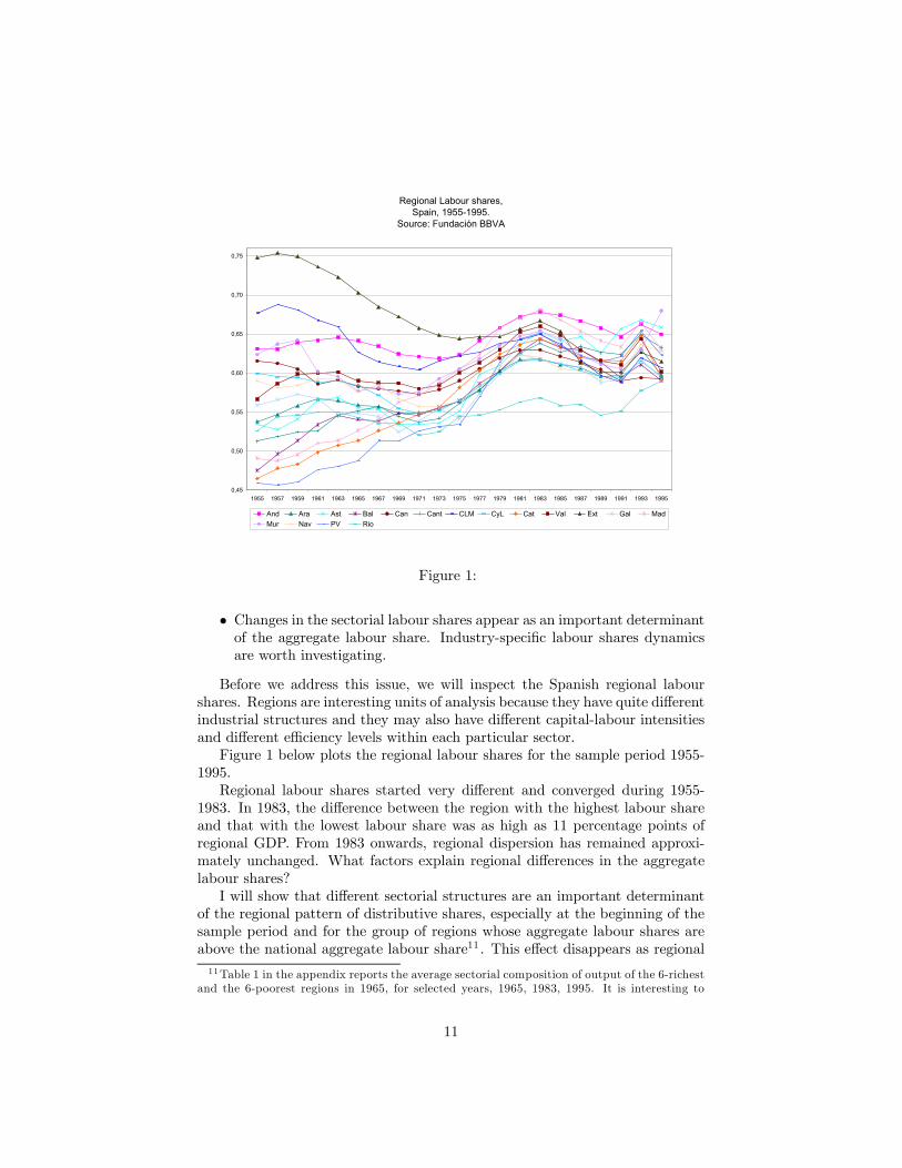
Regional Labour shares, Spain, 1955-1995.

Source: Fundación BBVA

0,45

0,50

0,55

0,60

0,65

0,70

0,75

1955 1957 1959 1961 1963 1965 1967 1969 1971 1973 1975 1977 1979 1981 1983 1985 1987 1989 1991 1993 1995

And Ara Ast Bal Can Cant CLM CyL Cat Val Ext Gal MadMur Nav PV Rio

Figure 1:

• Changes in the sectorial labour shares appear as an important determinantof the aggregate labour share. Industry-specific labour shares dynamicsare worth investigating.

Before we address this issue, we will inspect the Spanish regional labourshares. Regions are interesting units of analysis because they have quite differentindustrial structures and they may also have different capital-labour intensitiesand different efficiency levels within each particular sector.Figure 1 below plots the regional labour shares for the sample period 1955-

1995.Regional labour shares started very different and converged during 1955-

1983. In 1983, the difference between the region with the highest labour shareand that with the lowest labour share was as high as 11 percentage points ofregional GDP. From 1983 onwards, regional dispersion has remained approxi-mately unchanged. What factors explain regional differences in the aggregatelabour shares?I will show that different sectorial structures are an important determinant

of the regional pattern of distributive shares, especially at the beginning of thesample period and for the group of regions whose aggregate labour shares areabove the national aggregate labour share11 . This effect disappears as regional11Table 1 in the appendix reports the average sectorial composition of output of the 6-richest

and the 6-poorest regions in 1965, for selected years, 1965, 1983, 1995. It is interesting to

11

industrial structures converge. Comparative advantage in terms of industriallabour shares, i.e., regional industrial labour shares below the national value,becomes the most important determinant of the relative stability of regionallabour shares once industrial structures have converged. Comparative advantageis also the main determinant of the relative stability of the aggregate labourshares of the regions whose aggregate labour shares are below the national labourshare.We break down the difference between each region’s aggregate labour share

and the national aggregate labour share into three components: differences inthe sectorial composition of output, differences in the sectors’ labour shares anda covariance component, the joint effect of differences in the sectorial structureand differences in the industrial labour shares.Suppose each regional economy j is divided into N industries (i = 1...N),

with labour shares LSjit,∀j = 1...17, i = 1...N, t = 1...T , and weights in to-tal value added ωjit,∀j = 1...17, i = 1...N, t = 1...T . The labour shares andweights are observed over T time periods. The regional aggregate labour shareis computed as:

LSjt =NXi=1

ωjit · LSjit

Let LSt be the national aggregate labour share and LSit be sector i labourshare at the national level. Then, the difference between region’s j aggregatelabour share and the national aggregate labour share at time t can be decom-posed into three components:

LSjt − LSt =NXi=1

ωjit · LSjit −NXi=1

ωit · LSit =

=NXi=1

³ωjit − ωit

´· LSit +

+NXi=1

ωit ·³LSjit − LSit

´+

+NXi=1

³ωjit − ωit

´·³LSjit − LSit

´The first term measures the effect of differences in the sectorial composi-

tion of output on the difference between regional and national aggregate labourshares, holding the industrial labour shares constant at their national values.

notice that the 6 poorest regions in 1965 were also the regions whose aggregate labour shareswere above the national aggregate labour share in 1965. These were: Andalucía, Castilla-La-Mancha, Castilla y León, Extremadura, Galicia and Murcia. Four out of the 6 richest regionsin 1965 were also among the regions whose aggregate labour shares were below the nationallabour share in 1965. These were: Baleares, Cataluña, Madrid, País Vasco.

12

The second term measures the effect of differences in the industrial labour shareson the difference between regional and national aggregate shares, holding sec-tors’ value added shares at their national values. Finally, the last term measuresthe contribution of the interaction of differences in the sectorial composition ofoutput and differences in the sectorial labour shares.We perform this decomposition analysis for three years in the sample period:

1965, 1983 and 1995. For each of these years, regions are grouped into regionswhose aggregate labour shares were above the national labour share and regionswhose aggregate labour shares were below the national labour share. Table 5presents average results of this decomposition analysis for each group of regions.

TABLE 5.- Decomposition of differences in the regional labour shares

Year 1965 1983 1995Regions whose labour shares are ABOVE the national labour share(1)

Sectorial composition 24% 28% 15%Comparative advantage 43% 35% 42%Covariance 33% 38% 43%

Regions whose labour shares are BELOW the national labour share(2)

Sectorial composition -1% 7% -12%Comparative advantage 69% 63% 57%Covariance 31% 30% 56%

Note: (1) In 1965: Andalucía, Canarias, Castilla-La-Mancha, Castilla y León, ValenciaExtremadura, Galicia. In 1983: Andalucía, Valencia, Extremadura, Madrid.In 1995: Andalucía, Asturias, Murcia, Navarra, País Vasco. (2) In 1965: Baleares,Cantabria, Cataluña, Madrid, País Vasco, La Rioja. In 1983: Aragón, Baleares, Canarias, C-L-M, CyL, Cataluña, Galicia, Navarra, País Vasco, La Rioja. In 1995: Aragón, Baleares, Canarias, C-L-M, CyL, Cataluña, Valencia, Galicia, La Rioja.

In 1965, differences in the sectorial composition of output are important toexplain greater than national labour shares. Regions whose aggregate labourshares are greater than the national labour share are specialized in agriculture(whose average labour share is high), and they are not specialized in industry(whose aggregate labour share is low). Their lack of specialization in industry isagain the source of positive differences with respect to the national labour sharein 1983. On the contrary, the sectorial composition of output of the regionswhose aggregate labour shares are below the national share is not particularlyrelevant to explain the difference. Lower than national aggregate labour shareis due to their comparative advantage in terms of industrial labour shares. Thecovariance term plays an important role in 1995, for both types of regions. Re-gions whose labour shares are above the national are specialized in sectors wherethey have "comparative disadvantage" in terms of labour shares. On the con-trary, regions whose aggregate labour shares are below average are specializedin sectors where they have comparative advantage.The lessons we draw from this static decomposition analysis confirm our

previous findings:

• In summary, there are two margins to hold the regional labour shares

13

"relatively stable": one is the sectorial reallocation of resources and theother is the "relative stability" of the industrial labour shares.

• As development proceeds, the first margin becomes less important at thepresent level of sectorial disaggregation12.

Now, we turn to the second important determinant of the "relative stability"of the aggregate labour share: the relative stability of its industrial components.Table 2 in the appendix shows the labour share of income in each of the fifteen

sectors into which we divided the Spanish private productive sector13. Figure1 in the appendix plots these figures. Medium term and long-run fluctuationsare large (more than ten percentage points) and persistent. The statisticalhypothesis that the average value of any of these sectorial labour shares hasbeen constant over successive time intervals (1955-1975 and 1977-1995) is easilyrejected. Additionally, short-run fluctuations around a constant long-run valueare found to be first-order autoregresive. Also, the business cycle component ofthe sectorial labour shares is found to be countercyclical i.e., when the sectorialvalue added rises, the labour share declines1415.Let us focus for now at the medium and long-run oscillations. In all sectors,

the period 1955-1995 is characterized by a long-run accumulation of capitalrelative to labour. At the same time, nearly all sectors had increasing labourshares16. These two facts suggest that the elasticities of substitution of the sec-torial production functions must have been smaller than one. More precisely,assume each sector has a Constant Elasticity of Substitution production funtionand faces perfectly competitive good and factors’ markets and labour augment-ing technical progress accruing at a constant rate (which may be different sectorby sector). Then, the kind of trend increase experienced by most sectorial labourshares would result from the adjustment of relative factor quantities and fac-tor prices, for σi < 1 (σi represents the elasticity of substitution between thefactors). Let the CES production function in sector i be:

Yit = F (Kit,eLit) = haiK−ρiit + (1− ai) eL−ρiit

i− 1ρi , 0 < ai < 1,−1 ≤ ρi ≤ ∞

12Most probably, sectorial reallocation of resources would appear to have a relevant effecton the aggregate labour share if we looked at more disaggregated data and data measured athigher frequencies, monthly or quarterly data.13These are: C1. Agriculture and Fishing, C2. Fuel and power products, C3. Ferrous

and non-ferrous ores and metals, C4. Non-metallic minerals and minerals’ products, C5.Chemical products, C6. Metal products and machinery, C7. Transport equipment, C8. Food,beverages and tobacco, C9. Textiles and clothing, leather and footwear, C10. Paper andprinting products, C11. Rubber and plastic products and other manufactures, C12. Building,C13. Transport and communication services, C14. Financial and insurance services, C16.Residual of private productive services (includes: Recovery and repair services, Wholesale,Lodging and catering services, rest of private productive services).14The business cycle component of the labour share series was computed applying the

Hodrick-Prescott filter. The same results obtain if first-differenced logs of the labour shareare used instead.15The results of the statistical tests are available on request.16The exceptions being: Agriculture and Fishing, whose labour share declined over 1955-

1995 and Energy and power products and Financial and insurance services, whose labourshares exhibited a huge oscillation, first increasing then decreasing.

14

where eL represents labour measured in efficiency units. Then, σi = 11+ρi

.

Previous proposition is easily testable17 . First, we need to estimate thevalue of the elasticity of substitution of these CES production functions. Thiswe do under the assumption that labour-augmenting technical progress comesat a constant rate equal to the average growth rate of the estimated sectorialseries of Harrod-neutral technical progress18 . The point estimates range inthe interval [0.46; 0.86]19. The four big sectors (our previous five big sectors,excluding agriculture) have elasticities: 0.86 (Energy), 0.41 (Industry, excludingEnergy and Building), 0.58 (Building) and 0.81 (Private productive services).These estimated values may account for the long-run evolution of the sectoriallabour shares.Now, assume we want to test the ability of the model to reproduce the

behaviour of the sectorial labour shares over shorter time intervals. Sectoriallabour shares experience persistent deviations from their long-run values. Someshock must be causing these deviations. Consider, the following hypothesis:there are technical shocks (possibly biased and with some degree of persistence)hitting each sector every period. Hence, the capital-labour ratios (in efficiencyunits) adjust to these shocks and these adjustments cause observed fluctuationsof the labour shares. To test this hypothesis, we derive the series of biasedtechnical shocks directly from the estimated series of Harrod-neutral technicalprogress. At time t, each "sector/firm" i observes the shock, which affects theratio of marginal productivities of the factors, and chooses its capital-labourratio (in efficiency units) according to the profit-maximizing rule:

ekit = KiteLit = g(wit

rit, Bit) =

·ai

1− ai

wit

rit

1

Bit

¸where ek represents the capital-labour ratio measured in efficiency units andeL represents labour in efficiency units. Then, the labour share in sector i is

simply:

(1− αit) = 1− ai

ai + (1− ai)ekρiit17 In what follows, I briefly summarize the procedure and results of such a test, which are

described in full detail in section 2.6 of my dissertation.18Harrod-neutral technical progress is calculated dividing the Solow residual by the instan-

taneous labour share of income, i.e.,

Bit =1

(1− αit)

·µ∆Y

Y

¶it

− αit

µ∆K

K

¶it

− (1− αit)

µ∆L

L

¶it

¸19Except for agriculture, whose estimated elasticity of substitution is greater than one (1.82),

and two other sectors, whose estimated elasticities of substitution are too extreme to yield"reasonable" results in the simulation exercise that follows. These are: C7, 0.22 and C6, 4.7.

15

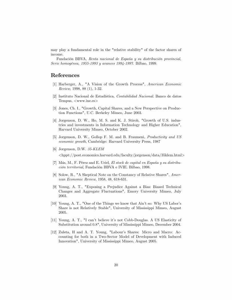
We checked this hypothesis for every sector where it was possible20 . For thesake of brevity, we report results for the biggest sectors only: industry, servicesand building21. These results are quite general. In fact, the finer the sectorialdisaggregation, the more explicit the differences between actual and simulatedlabour share series are. Figures 1 to 3 in the appendix plot actual and modellabour share series. Simulated labour shares do not match the huge fluctuationsactually experienced by the sectors’ labour shares. In the services sector, actuallabour share grows by ten percentage points more than predicted by the modelfrom 1965 to 1983 and falls also more, by 6 percentage points, during 1983-1995. In the building sector, there is a difference of approximately 5 percentagepoints between actual and simulated series, first in their way up, then in theirway down. In industry, actual labour share grows by 5 percentage points morethan predicted by the model during 1965-1983. The model predictions are quiteaccurate for the period 1983-1995.Even after taking into account the effect of varying growth rates of technical

progress, the model is unable to reproduce medium term dynamics of the sec-torial labour shares. The model misses the factors explaining why the labourshares grew more than predicted and why they also fell more. It would seem asif the elasticities of substitution had been initially lower than estimated long-run values. At some point (around 1983), the elasticity of substitution reachesits long-run value as in the industrial sector or an even greater value as in theservices sector. In the building sector, the factor price actually decreased during1983-1995 while the capital-labour ratio remained approximately constant.At the aggregate level, we have documented a trend increase in the labour

share, of approximately 7 percentage points -sample period 1955-1995-, 5 per-centage points if we focus on the sample period 1971-1995. The capital-labourratio increased by 184% over 1971-1995 or equivalently at an annual rate equalto 4.44%. The puzzling feature of the aggregate picture is that during 1983-1995, when the labour share declined at an annual rate equal to 0.5%, thecapital-labour ratio increased at an annual rate equal to 3.1%. During the pe-riod 1971-1983, the labour share rose by 1.2% annually while the capital-labourratio increased by 5.8% per year. A look at the series of Harrod-neutral technicalprogress shows two periods of very high positive rates of technical improvement,from 1965 to 1973 and from 1983 to 1989 (Figure 4 in the appendix). The jumpin the growth rate of technical progress from 1983 onwards may explain thedecline in the labour share in the face of a rising capital-labour ratio.Within any given sector, a rising labour share of income automatically im-

plies a declining capital share and if the capital-output ratio does not adjust,declining returns on investments. In the face of a very low elasticity of substi-

20Using Spanish data, we computed the model labour shares for each of the following sectors:C1, C2, C4, C6, C7, C9, C10, C11, C12, C14 and C16.21The two excluded sectors are: energy and agriculture. The energy sector has been char-

acterized for the greatest part of the sample period by a market structure close to monopoly.Agriculture seems to be a sector with a fully different pattern of behaviour. There is a cleardownward trend of the labour share, interrupted at the end of the sample period. Here onemay suspect that there are European and Spanish social funds reversing the falling trend ofthe labour share.

16

tution or even a putty-clay technology, firms/sectors may try to introduce newtechnologies that save on the expensive factor (as far as these are available)and/or may slowly substitute capital for labour. Both strategies would lead toan increase of the income share of capital.Hence, from the sectorial evidence, the lessons we draw are:

• Medium run dynamics do not follow the logic of the model with CESproduction function plus varying rates of technical progress and at thesame time, they seem key to understand the pattern of behaviour of thelabour shares, their relative stability. That is, the labour shares rise andin response, efforts are made to force these shares down.

• Induced and biased technical improvement may play an important role asa mechanism to guarantee the relative stability of the industrial labourshares.

4 US EvidenceTable 3 in the appendix shows the share of labour in total income generated inthe US private sector over 1958-1996 (annual data), at the aggregate level andfor each of five big sectors. The shares were calculated from data included inthe 35-KLEM data set downloaded from Professor Dale Jorgenson’s web page.Aggregate labour share is the weighted average of the sectorial shares, withweights equal to the sectors’ value added shares. Sectors’ labour shares werecomputed as the ratio of the value of the labour services to the sector’s valueadded, both measured in current Million dollars22.The aggregate labour share shows a very slight downward trend, which is

not statistically significant. The labour share represented 69% of total incomein 1958 and 67% in 1996. Short-run fluctuations of the aggregate labour sharerange in the interval [0.65; 0.70].The sectors’ labour shares are substantially different and these differences

are highly persistent. Although fluctuations of the US sectorial labour shares arenot as important as their Spanish counterparts, they are larger than observedfluctuations at the aggregate level. They turn around 10 percentage points ofsectorial value added.Table 4 in the appendix reports sectors’ value added shares during 1958-

1996. By 1958, when our times series start, the structural change in the USwas almost completed. Agriculture’s share of total value added was only 6%,industry’s share was 30% and the private services’ share was 54%. During theperiod 1958-1974, these shares remained stable. Also the aggregate labour sharechanged by less than half a percentage point. During 1975-1996, the share ofindustry went down to 25% of total value added while the share of services

22The methodology used to construct the 35-KLEM database is described in Jorgenson etal (1987) and Jorgenson et al (2002). The estimated values of the labour services alreadyinclude a correction for the labour earnings of the self-employed. No data are available on thecomposition of the workforce (ratio of employees/ total employment).

17

increased to 65%. The aggregate labour share decreased by 2 percentage pointsduring this interval. Table 6 quantifies the effect of both the changes in thesectorial composition of output and the changes in the sectorial labour shareson the aggregate labour share.

TABLE 6.- Decomposition of changes in aggregate labour share, in percentage termsUS, 1958-1996

Sample period 1958-1974 1975-1996

Changes in sectorial composition -153% -6%

Changes in sectors' labour shares 195% 123%

Covariance term 58% -17%

Changes in aggregate labour share 0,4 p.p -2,3 p.p.

During 1958-1974, the decrease of agriculture’s share of total value addedaccounts for the negative effect of the changes in the sectorial composition ofoutput on the aggregate labour share’s growth. During 1975-1996, a decreasingindustrial share of value added helped reduce the aggregate labour share but thiseffect was more than compensated by the increase in the services share of valueadded. Overall, the main determinant of observed evolution of the aggregatelabour share are the changes in the sectorial labour shares. In particular, during1975-1996, the labour share decreased in all big sectors, the exception being thebuilding sector.The covariance term does not play a meaningful role. We checked correla-

tions between changes in the sectorial labour shares. First, we recomputed afixed-weight aggregate labour share, using the weights of 1985. The varianceof this fixed-weight aggregate labour share turns out to be 0.0001359. Next,we computed the theoretical variance of the aggregate labour share, under theassumption that the sector labour shares moved independently in a statisti-cal sense. This variance is equal to 0.0001374. Hence, the US sector sharesfluctuated almost independently during 1958-1996.Let us now focus on the pattern of the sectors’ labour shares. Table 5 in the

appendix shows the labour share of income in each of the fifteen sectors intowhich we divided the US private sector23. Figure 6 in the appendix plots thesefigures. As in Spain, medium term and long-run fluctuations are large (morethan ten percentage points) and persistent. The statistical hypothesis that theaverage value of any of these sectorial labour shares has been constant over suc-cessive time intervals (1958-1975 and 1976-1996) is rejected in all sectors, withthe exception of sectors C7, C10, C12, C13. Additionally, short-run fluctuationsaround a constant long-run value are found to be first-order autoregresive. Andalso as in Spain, the business cycle component of the US sectors labour shares

23These are comparable to the 15 sectors into which we divided the Spanih private produc-tive sector except for C14, which includes Real Estate in the US, but not in Spain.

18

is countercyclical2425. However, what we called "medium-term" oscillations ofthe sector shares are much shorter in the US than they are in Spain.How does the model with CES production function and varying growth rates

of the labour-augmenting technical progress perform in the US? First, we es-timated elasticities of substitution of the sectorial production functions. Thepoint estimates fell in the range [0.15; 0.78] if we exclude the sectors whose elas-ticities were too close to one26. Next, we simulated each sector labour shareseries under the assumption that firms/sectors observe "true" technical shocksand adjust their capital-labour ratios, measured in efficiency units, accordingly.The model labour shares reproduce quite accurately the actual labour shares insome of the manufacturing sectors (C5, C6, C7) and one of the services sectors,C14. However, the model labour shares generally fail to account for all of theobserved variability of the sector labour shares. Actual short-run fluctuationsof the sector shares are larger than those predicted by the model. Actual sectorlabour shares grow more and they also fall more than their model counterparts.

5 Concluding remarksThis paper has evaluated the "relative constancy" of the aggregate labour sharefrom a new perspective with suggestive and challenging results.Changes in the aggregate labour share are found to be quantitatively relevant

in Spain, much less so in the US. Changes in the industrial labour shares arefound to be quantitatively relevant both in Spain and in the US. However,our main finding is that changes in the labour shares, be it at the aggregate orsectorial levels, in Spain or in the US, may be explained in terms of an analyticalframework that embodies well-established economic principles.Based on the examination of sectorial and regional data as well as aggregate

data, we are able to suggest an empirically testable explanation of the fact thatvarious industries with widely-oscillating labour shares integrate an economywith a "relatively constant" aggregate labour share. The relative stability of theaggregate labour share is due to deliberate efforts on the part of firms/sectors toreduce the labour share of income as much as possible, given existing technicalrestrictions, factor supply conditions and commodity demand conditions. Suchefforts may take the form of changes in the input ratios used in production,adoption of new labour saving technologies or reallocation of resources to sectorswhose labour shares are lower.If such an hypothesis is tested and accepted, it is not without important

implications for models of growth and business cycles. Movements in the labourshares become central to understand and explain cyclical fluctuations of outputand even its long-run growth rate since endogenous and biased technical progress

24The business cycle component is computed both by HP detrending the labour share seriesand by first-differencing the log of the series. Both detrending methods yield comparableresults.25Results of the statistical tests are available on request.26These sectors are: C2, C3, C7, C9, C12, with elasticities: 1.19; 0.83; 0.86; 0.92; 0.94. These

sectors perform poorly in the simulations of the model labour shares.

19

may play a fundamental role in the "relative stability" of the factor shares ofincome.Fundación BBVA, Renta nacional de España y su distribución provincial,

Serie homogénea, 1955-1993 y avances 1994-1997. Bilbao, 1999.

References[1] Harberger, A., "A Vision of the Growth Process", American Economic

Review, 1998, 88 (1), 1-32.

[2] Instituto Nacional de Estadística, Contabilidad Nacional. Banco de datosTempus, <www.ine.es>

[3] Jones, Ch. I., "Growth, Capital Shares, and a New Perspective on Produc-tion Functions", U.C. Berkeley Mimeo, June 2003.

[4] Jorgenson, D. W., Ho, M. S. and K. J. Stiroh, "Growth of U.S. indus-tries and investments in Information Technology and Higher Education",Harvard University Mimeo, October 2002.

[5] Jorgenson, D. W., Gollop F. M. and B. Fraumeni, Productivity and USeconomic growth, Cambridge: Harvard University Press, 1987

[6] Jorgenson, D.W. 35-KLEM

<hppt://post.economics.harvard.edu/faculty/jorgenson/data/35klem.html>

[7] Más, M., F. Pérez and E. Uriel, El stock de capital en España y su distribu-ción territorial, Fundación BBVA e IVIE. Bilbao, 1998.

[8] Solow, R., "A Skeptical Note on the Constancy of Relative Shares", Amer-ican Economic Review, 1958, 48, 618-631.

[9] Young, A. T., "Exposing a Prejudice Against a Bias: Biased TechnicalChanges and Aggregate Fluctuations", Emory University Mimeo, July2003.

[10] Young, A. T., "One of the Things we know that Ain’t so: Why US Labor’sShare is not Relatively Stable", University of Mississippi Mimeo, August2005.

[11] Young, A. T., "I can’t believe it’s not Cobb-Douglas. A US Elasticity ofSubstitution around 0.8", University of Mississippi Mimeo, December 2004.

[12] Zuleta, H and A. T. Young, "Labour’s Shares: Micro and Macro: Ac-counting for both in a Two-Sector Model of Development with InducedInnovation", University of Mississippi Mimeo, August 2005.

20

A Tables

A.1 Sectorial composition of output in Spain

TABLE 1.- Sectorial composition of output in Spain for selected years, 1965, 1983, 19951965

A&F Energy Industry Building Services6 poorest regions in 1965 0,33 0,07 0,19 0,09 0,336 richest regions in 1965 0,13 0,03 0,35 0,09 0,40National 0,17 0,05 0,29 0,08 0,41

1983A&F Energy Industry Building Services

6 poorest regions in 1965 0,17 0,06 0,23 0,11 0,446 richest regions in 1965 0,05 0,03 0,34 0,07 0,51National 0,08 0,04 0,29 0,08 0,52

1995A&F Energy Industry Building Services

6 poorest regions in 1965 0,12 0,07 0,18 0,13 0,496 richest regions in 1965 0,03 0,03 0,26 0,09 0,59National 0,06 0,04 0,21 0,09 0,60Note: A&F represents agriculture and fishing; Services represents the private productive services i.e., government and Real Estate excluded.Note: 6 poorest regions in 1965: Andalucía, Castilla-La-Mancha, Castilla y León, Extremadura, Galicia,Murcia. 6 richest regions in 1965: Baleares, Cataluña, Madrid, Navarra, País Vasco, Valencia.

21

A.2 Sectorial labour shares in Spain (15 sectors)

TABLE 2.- Sectorial Labour shares in Spain, 1955-1995

Sector C1 C2 C3 C4 C5 C6 C7 C8 C9 C10 C11 C12 C13 C14 C16Year1955 0,79 0,28 0,52 0,46 0,29 0,46 0,40 0,48 0,38 0,51 0,39 0,71 0,50 0,45 0,501957 0,80 0,26 0,51 0,45 0,28 0,47 0,42 0,49 0,41 0,52 0,42 0,71 0,52 0,42 0,501959 0,80 0,27 0,50 0,43 0,29 0,47 0,43 0,49 0,42 0,49 0,45 0,71 0,52 0,45 0,511961 0,80 0,26 0,53 0,45 0,31 0,50 0,42 0,51 0,43 0,48 0,48 0,71 0,56 0,53 0,501963 0,78 0,28 0,52 0,55 0,33 0,49 0,44 0,52 0,44 0,50 0,51 0,69 0,59 0,46 0,501965 0,76 0,29 0,48 0,50 0,35 0,50 0,50 0,52 0,44 0,52 0,55 0,67 0,62 0,50 0,501967 0,74 0,29 0,56 0,43 0,36 0,56 0,52 0,54 0,45 0,52 0,57 0,68 0,64 0,50 0,511969 0,70 0,26 0,50 0,46 0,37 0,58 0,52 0,54 0,47 0,55 0,55 0,68 0,64 0,56 0,521971 0,70 0,26 0,52 0,43 0,38 0,62 0,55 0,55 0,48 0,52 0,51 0,70 0,62 0,56 0,531973 0,70 0,29 0,47 0,41 0,40 0,61 0,52 0,57 0,50 0,52 0,49 0,70 0,61 0,62 0,541975 0,68 0,30 0,40 0,45 0,43 0,61 0,56 0,60 0,55 0,52 0,59 0,71 0,63 0,61 0,551977 0,67 0,36 0,44 0,43 0,47 0,62 0,66 0,57 0,56 0,53 0,58 0,75 0,65 0,62 0,581979 0,65 0,36 0,51 0,44 0,52 0,67 0,74 0,55 0,63 0,61 0,58 0,77 0,69 0,65 0,591981 0,61 0,36 0,56 0,51 0,53 0,72 0,73 0,55 0,63 0,71 0,65 0,86 0,73 0,55 0,611983 0,61 0,37 0,56 0,54 0,51 0,69 0,72 0,54 0,59 0,64 0,69 0,88 0,75 0,63 0,631985 0,62 0,35 0,53 0,55 0,47 0,66 0,76 0,58 0,60 0,65 0,69 0,85 0,73 0,56 0,621987 0,61 0,30 0,60 0,53 0,47 0,64 0,70 0,58 0,59 0,64 0,66 0,83 0,73 0,55 0,621989 0,63 0,28 0,58 0,47 0,49 0,67 0,69 0,53 0,57 0,67 0,69 0,75 0,74 0,50 0,611991 0,64 0,30 0,72 0,46 0,58 0,69 0,73 0,54 0,61 0,68 0,69 0,70 0,76 0,49 0,591993 0,66 0,29 0,80 0,57 0,66 0,76 0,84 0,55 0,76 0,78 0,83 0,79 0,79 0,51 0,591995 0,70 0,28 0,79 0,50 0,60 0,70 0,72 0,58 0,70 0,59 0,75 0,74 0,77 0,46 0,57

Note: C1. Agriculture and Fishing, C2. Fuel and power products, C3. Ferrous and non-ferrous ores and metals, C4. Non-metallic minerals and minerals' products, C5. Chemical products, C6. Metal products and machinery, C7. Transport equipment, C8. Food, beverages and tobacco, C9. Textiles and clothing, leather and footwear, C10. Paper and printing products, C11. Rubber and plastic products and other manufactures, C12. Building, C13. Transport and communication services, C14. Financial and insurance services, C16. Residual of private productive services.

22

A.3 Private sector and 5 big sectors’ Labour shares, US

TABLE 3.- Aggregate and 5 big sectors' Labour shares in the US, 1958-1996Sector A&F E I B S TotalYear1958 0,79 0,43 0,75 0,88 0,64 0,691959 0,76 0,43 0,72 0,90 0,63 0,681960 0,75 0,43 0,74 0,92 0,64 0,691961 0,75 0,44 0,74 0,91 0,64 0,691962 0,75 0,44 0,73 0,90 0,63 0,681963 0,68 0,43 0,72 0,90 0,64 0,681964 0,71 0,42 0,71 0,89 0,63 0,671965 0,65 0,40 0,70 0,88 0,62 0,661966 0,63 0,39 0,70 0,87 0,61 0,651967 0,68 0,39 0,72 0,87 0,61 0,661968 0,73 0,41 0,72 0,88 0,62 0,671969 0,68 0,44 0,73 0,88 0,64 0,681970 0,70 0,41 0,76 0,88 0,64 0,691971 0,69 0,41 0,74 0,87 0,63 0,681972 0,65 0,43 0,73 0,88 0,64 0,681973 0,55 0,41 0,74 0,89 0,65 0,691974 0,60 0,37 0,77 0,90 0,66 0,701975 0,71 0,41 0,73 0,87 0,67 0,691976 0,67 0,39 0,73 0,86 0,64 0,671977 0,65 0,41 0,73 0,86 0,63 0,671978 0,64 0,41 0,74 0,87 0,64 0,671979 0,62 0,36 0,76 0,86 0,64 0,681980 0,62 0,34 0,77 0,86 0,65 0,691981 0,60 0,34 0,76 0,88 0,67 0,691982 0,58 0,34 0,76 0,89 0,67 0,691983 0,62 0,32 0,74 0,87 0,63 0,661984 0,58 0,34 0,73 0,90 0,66 0,671985 0,61 0,34 0,73 0,90 0,65 0,681986 0,63 0,42 0,73 0,87 0,64 0,671987 0,51 0,37 0,71 0,90 0,65 0,681988 0,52 0,32 0,71 0,92 0,68 0,691989 0,58 0,32 0,71 0,87 0,66 0,681990 0,59 0,29 0,71 0,88 0,66 0,671991 0,64 0,36 0,71 0,89 0,64 0,671992 0,66 0,40 0,71 0,88 0,64 0,671993 0,64 0,39 0,71 0,88 0,64 0,661994 0,63 0,40 0,69 0,89 0,64 0,661995 0,61 0,40 0,68 0,90 0,65 0,671996 0,59 0,36 0,67 0,91 0,66 0,67

Note: A&F represents agriculture and fishing; E: energy; I: industry; B: building; S: the private services,i.e., government excluded.

23

A.4 Sectors’ value added shares in the USTABLE 4.- Sectors' value added shares in the US, 1958-1996

Sector A&F E I B SYear1958 0,06 0,03 0,30 0,07 0,541959 0,05 0,03 0,31 0,07 0,541960 0,05 0,03 0,31 0,07 0,541961 0,05 0,03 0,30 0,07 0,551962 0,05 0,03 0,31 0,07 0,551963 0,04 0,03 0,31 0,08 0,551964 0,04 0,02 0,31 0,08 0,551965 0,04 0,02 0,31 0,08 0,551966 0,04 0,02 0,31 0,08 0,551967 0,04 0,02 0,31 0,07 0,551968 0,04 0,02 0,31 0,08 0,551969 0,04 0,02 0,31 0,08 0,561970 0,04 0,02 0,29 0,08 0,581971 0,04 0,02 0,28 0,08 0,581972 0,04 0,02 0,28 0,08 0,581973 0,05 0,02 0,29 0,08 0,561974 0,04 0,04 0,30 0,07 0,551975 0,04 0,05 0,29 0,07 0,561976 0,04 0,05 0,30 0,07 0,541977 0,03 0,04 0,31 0,07 0,541978 0,03 0,04 0,31 0,07 0,541979 0,03 0,04 0,31 0,07 0,531980 0,03 0,05 0,30 0,07 0,541981 0,03 0,06 0,30 0,06 0,551982 0,03 0,06 0,28 0,06 0,571983 0,02 0,05 0,27 0,06 0,591984 0,03 0,05 0,28 0,06 0,591985 0,02 0,04 0,27 0,07 0,591986 0,02 0,03 0,27 0,07 0,611987 0,02 0,03 0,27 0,07 0,611988 0,02 0,03 0,27 0,07 0,611989 0,02 0,03 0,26 0,07 0,621990 0,02 0,03 0,25 0,06 0,631991 0,02 0,03 0,25 0,06 0,641992 0,02 0,02 0,25 0,06 0,651993 0,03 0,02 0,25 0,06 0,651994 0,02 0,02 0,25 0,06 0,651995 0,02 0,02 0,25 0,05 0,651996 0,02 0,02 0,25 0,05 0,65

Note: Value added shares are computed as GVAit/ΣGVAit for all i=1...5, where grossvalue added are measured in current terms.

24

A.5 Sectorial labour shares in the US (15 sectors)

TABLE 5.- Sectorial Labour shares in the US, 1958-1996

Sector C1 C2 C3 C4 C5 C6 C7 C8 C9 C10 C11 C12 C13 C14 C16Year1958 0,79 0,43 0,55 0,65 0,56 0,76 0,85 0,70 0,88 0,73 0,78 0,88 0,57 0,41 0,741959 0,76 0,43 0,54 0,64 0,51 0,73 0,89 0,69 0,87 0,71 0,77 0,90 0,57 0,41 0,721960 0,75 0,43 0,58 0,66 0,55 0,75 0,91 0,71 0,87 0,73 0,80 0,92 0,56 0,40 0,751961 0,75 0,44 0,60 0,66 0,54 0,75 0,87 0,70 0,87 0,73 0,78 0,91 0,55 0,42 0,741962 0,75 0,44 0,57 0,66 0,54 0,73 0,86 0,69 0,86 0,73 0,78 0,90 0,55 0,43 0,721963 0,68 0,43 0,54 0,64 0,53 0,71 0,85 0,67 0,85 0,73 0,78 0,90 0,54 0,46 0,721964 0,71 0,42 0,51 0,64 0,53 0,71 0,85 0,68 0,85 0,71 0,78 0,89 0,54 0,45 0,711965 0,65 0,40 0,50 0,66 0,52 0,68 0,85 0,68 0,83 0,71 0,77 0,88 0,55 0,42 0,701966 0,63 0,39 0,48 0,68 0,54 0,69 0,87 0,67 0,82 0,70 0,79 0,87 0,55 0,38 0,691967 0,68 0,39 0,50 0,70 0,57 0,71 0,88 0,68 0,83 0,72 0,78 0,87 0,56 0,36 0,701968 0,73 0,41 0,54 0,70 0,55 0,71 0,88 0,68 0,84 0,72 0,76 0,88 0,56 0,40 0,711969 0,68 0,44 0,58 0,69 0,58 0,74 0,89 0,68 0,84 0,72 0,76 0,88 0,57 0,43 0,731970 0,70 0,41 0,62 0,73 0,59 0,78 0,89 0,67 0,83 0,75 0,81 0,88 0,58 0,41 0,731971 0,69 0,41 0,61 0,70 0,57 0,74 0,89 0,67 0,84 0,74 0,78 0,87 0,58 0,39 0,721972 0,65 0,43 0,58 0,70 0,56 0,73 0,91 0,70 0,83 0,73 0,76 0,88 0,59 0,42 0,721973 0,55 0,41 0,56 0,70 0,56 0,75 0,90 0,73 0,86 0,72 0,75 0,89 0,60 0,46 0,731974 0,60 0,37 0,49 0,74 0,58 0,81 0,90 0,73 0,86 0,73 0,80 0,90 0,60 0,46 0,741975 0,71 0,41 0,57 0,72 0,57 0,77 0,89 0,60 0,82 0,72 0,75 0,87 0,58 0,54 0,741976 0,67 0,39 0,59 0,71 0,55 0,76 0,89 0,65 0,84 0,71 0,75 0,86 0,58 0,47 0,721977 0,65 0,41 0,59 0,72 0,58 0,75 0,89 0,66 0,82 0,72 0,74 0,86 0,58 0,41 0,721978 0,64 0,41 0,56 0,70 0,59 0,75 0,89 0,68 0,83 0,74 0,75 0,87 0,58 0,43 0,731979 0,62 0,36 0,55 0,72 0,61 0,78 0,90 0,70 0,84 0,75 0,76 0,86 0,60 0,43 0,731980 0,62 0,34 0,56 0,74 0,65 0,78 0,91 0,69 0,83 0,76 0,80 0,86 0,59 0,45 0,741981 0,60 0,34 0,56 0,77 0,60 0,77 0,91 0,65 0,82 0,75 0,79 0,88 0,57 0,53 0,741982 0,58 0,34 0,50 0,76 0,63 0,79 0,91 0,62 0,81 0,73 0,77 0,89 0,56 0,55 0,741983 0,62 0,32 0,45 0,72 0,60 0,77 0,87 0,63 0,79 0,73 0,75 0,87 0,53 0,47 0,721984 0,58 0,34 0,44 0,72 0,60 0,75 0,86 0,61 0,82 0,72 0,75 0,90 0,53 0,52 0,741985 0,61 0,34 0,40 0,71 0,62 0,77 0,91 0,59 0,82 0,71 0,74 0,90 0,53 0,48 0,751986 0,63 0,42 0,39 0,65 0,61 0,77 0,93 0,59 0,79 0,70 0,73 0,87 0,53 0,47 0,731987 0,51 0,37 0,41 0,69 0,54 0,75 0,87 0,58 0,80 0,69 0,73 0,90 0,53 0,46 0,761988 0,52 0,32 0,45 0,74 0,53 0,75 0,89 0,57 0,80 0,68 0,75 0,92 0,52 0,51 0,781989 0,58 0,32 0,47 0,75 0,53 0,76 0,91 0,55 0,79 0,67 0,74 0,87 0,53 0,49 0,751990 0,59 0,29 0,53 0,76 0,56 0,75 0,91 0,52 0,79 0,70 0,75 0,88 0,55 0,45 0,751991 0,64 0,36 0,50 0,75 0,58 0,76 0,87 0,53 0,78 0,71 0,74 0,89 0,54 0,42 0,751992 0,66 0,40 0,51 0,76 0,58 0,76 0,87 0,53 0,76 0,72 0,75 0,88 0,55 0,43 0,741993 0,64 0,39 0,49 0,76 0,58 0,75 0,87 0,56 0,77 0,73 0,74 0,88 0,55 0,41 0,731994 0,63 0,40 0,54 0,74 0,54 0,73 0,87 0,54 0,78 0,71 0,74 0,89 0,55 0,44 0,731995 0,61 0,40 0,49 0,72 0,51 0,72 0,87 0,51 0,80 0,70 0,73 0,90 0,56 0,42 0,761996 0,59 0,36 0,52 0,71 0,52 0,71 0,87 0,50 0,78 0,70 0,71 0,91 0,57 0,42 0,76

Note: C1. Agriculture and Fishing, C2. Fuel and power products, C3. Ferrous and non-ferrous ores and metals, C4. Non-metallic minerals and minerals' products, C5. Chemical products, C6. Metal products and machinery, C7. Transport equipment, C8. Food, beverages and tobacco, C9. Textiles and clothing, leather and footwear, C10. Paper and printing products, C11. Rubber and plastic products and other manufactures, C12. Building, C13. Transport and communication services, C14. Finance and insurance services, and Real Estate, C16. Residual of private productive services.

25

B Figures

B.1 Sectors’ labour shares in Spain, 15 sectors

Figure 1

C1

0,60

0,65

0,70

0,75

0,80

0,85

0,90

1955 1961 1967 1973 1979 1985 1991

C2

0,20

0,25

0,30

0,35

0,40

0,45

0,50

1955 1961 1967 1973 1979 1985 1991

C3

0,35

0,45

0,55

0,65

0,75

0,85

1955 1961 1967 1973 1979 1985 1991

C4

0,35

0,40

0,45

0,50

0,55

0,60

0,65

1955 1961 1967 1973 1979 1985 1991

C5

0,25

0,35

0,45

0,55

0,65

1955 1961 1967 1973 1979 1985 1991

C6

0,40

0,50

0,60

0,70

0,80

1955 1961 1967 1973 1979 1985 1991

C7

0,35

0,45

0,55

0,65

0,75

0,85

1955 1961 1967 1973 1979 1985 1991

C8

0,40

0,45

0,50

0,55

0,60

0,65

0,70

1955 1961 1967 1973 1979 1985 1991

C9

0,35

0,45

0,55

0,65

0,75

1955 1961 1967 1973 1979 1985 1991

C10

0,450,500,550,600,650,700,750,80

1955 1961 1967 1973 1979 1985 1991

C11

0,35

0,45

0,55

0,65

0,75

0,85

1955 1961 1967 1973 1979 1985 1991

C12

0,65

0,70

0,75

0,80

0,85

0,90

0,95

1955 1961 1967 1973 1979 1985 1991

C13

0,50

0,55

0,60

0,65

0,70

0,75

0,80

1955 1961 1967 1973 1979 1985 1991

C14

0,40

0,45

0,50

0,55

0,60

0,65

0,70

1955 1961 1967 1973 1979 1985 1991

C16

0,40

0,45

0,50

0,55

0,60

0,65

0,70

1955 1961 1967 1973 1979 1985 1991

26

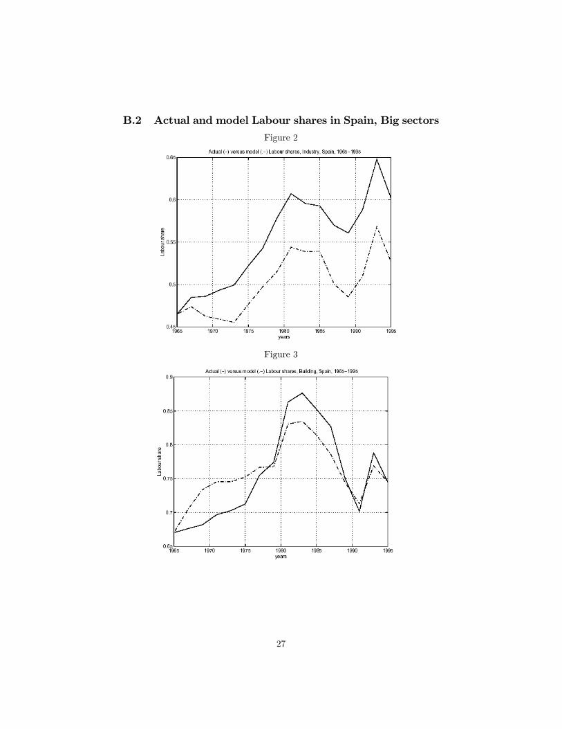
B.2 Actual and model Labour shares in Spain, Big sectorsFigure 2

Figure 3

27

Figure 4

B.3 Labour-augmenting technical progress in the privateproductive sector, Spain

Figure 5

Harrod-neutral technical progress growth rates, Private productive sector, Spain, 1965/67-1993/95

-6%

-4%

-2%

0%

2%

4%

6%

8%

10%

12%

14%

1967 1969 1971 1973 1975 1977 1979 1981 1983 1985 1987 1989 1991 1993 1995

Gro

wth

rate

s

28

B.4 Sectors’ labour shares in the US, 15 sectors

Figure 6

C1

0,500,550,600,650,700,750,800,85

1958 1964 1970 1976 1982 1988 1994

C2

0,25

0,30

0,35

0,40

0,45

0,50

0,55

1958 1964 1970 1976 1982 1988 1994

C3

0,35

0,40

0,45

0,50

0,55

0,60

0,65

1958 1964 1970 1976 1982 1988 1994

C4

0,55

0,60

0,65

0,70

0,75

0,80

0,85

1958 1964 1970 1976 1982 1988 1994

C5

0,40

0,45

0,50

0,55

0,60

0,65

0,70

1958 1964 1970 1976 1982 1988 1994

C6

0,60

0,65

0,70

0,75

0,80

0,85

0,90

1958 1964 1970 1976 1982 1988 1994

C7

0,65

0,70

0,75

0,80

0,85

0,90

0,95

1958 1964 1970 1976 1982 1988 1994

C8

0,45

0,50

0,55

0,60

0,65

0,70

0,75

1958 1964 1970 1976 1982 1988 1994

C9

0,65

0,70

0,75

0,80

0,85

0,90

0,95

1958 1964 1970 1976 1982 1988 1994

C10

0,55

0,60

0,65

0,70

0,75

0,80

0,85

1958 1964 1970 1976 1982 1988 1994

C11

0,65

0,70

0,75

0,80

0,85

0,90

0,95

1958 1964 1970 1976 1982 1988 1994

C12

0,65

0,70

0,75

0,80

0,85

0,90

0,95

1958 1964 1970 1976 1982 1988 1994

C13

0,40

0,45

0,50

0,55

0,60

0,65

0,70

1958 1964 1970 1976 1982 1988 1994

C14

0,30

0,35

0,40

0,45

0,50

0,55

0,60

1958 1964 1970 1976 1982 1988 1994

C16

0,55

0,60

0,65

0,70

0,75

0,80

0,85

1958 1964 1970 1976 1982 1988 199429