International Journal of Solids and Structures 90 (2016) 236–250

Contents lists available at ScienceDirect

International Journal of Solids and Structures

journal homepage: www.elsevier.com/locate/ijsolstr

Non-prismatic beams: A simple and effective Timoshenko-like model

Giuseppe Balduzzi a , ∗, Mehdi Aminbaghai b , Elio Sacco

c , Josef Füssl b , Josef Eberhardsteiner b , Ferdinando Auricchio

a

a Department of Civil Engineering and Architeture (DICAr), University of Pavia, Pavia 27100, Italy b Institute for Mechanics of Materials and Structures (IMWS), Vienna University of Technology, Vienna, Austria c Department of Civil and Mechanical Engineering, University of Cassino and Southern Lazio, Cassino, Italy

a r t i c l e i n f o

Article history:

Received 3 July 2015

Revised 2 February 2016

Available online 19 February 2016

Keywords:

Non-prismatic Timoshenko beam

Beam modeling

Analytical solution

Tapered beam

Arches

a b s t r a c t

The present paper discusses simple compatibility, equilibrium, and constitutive equations for a non-

prismatic planar beam. Specifically, the proposed model is based on standard Timoshenko kinematics

(i.e., planar cross-section remain planar in consequence of a deformation, but can rotate with respect to

the beam center-line). An initial discussion of a 2D elastic problem highlights that the boundary equilib-

rium deeply influences the cross-section stress distribution and all unknown fields are represented with

respect to global Cartesian coordinates. A simple beam model (i.e. a set of Ordinary Differential Equa-

tions (ODEs)) is derived, describing accurately the effects of non-prismatic geometry on the beam be-

havior and motivating equation’s terms with both physical and mathematical arguments. Finally, several

analytical and numerical solutions are compared with results existing in literature. The main conclusions

can be summarized as follows. (i) The stress distribution within the cross-section is not trivial as in pris-

matic beams, in particular the shear stress distribution depends on all generalized stresses and on the

beam geometry. (ii) The derivation of simplified constitutive relations highlights a strong dependence of

each generalized deformation on all the generalized stresses. (iii) Axial and shear-bending problems are

strictly coupled. (iv) The beam model is naturally expressed as an explicit system of six first order ODEs.

(v) The ODEs solution can be obtained through the iterative integration of the right hand side term of

each equation. (vi) The proposed simple model predicts the real behavior of non-prismatic beams with a

good accuracy, reasonable for the most of practical applications.

© 2016 Elsevier Ltd. All rights reserved.

r

e

t

l

d

t

1. Introduction

Non-prismatic beams –sometime mentioned also as beams with

non-constant cross-section or beams of variable cross-section – are a

particular class of slender bodies, object of the practitioners inter-

est due to the possibility of optimizing their geometry with respect

to specific needs ( Auricchio et al., 2015; Timoshenko and Young,

1965 ). Despite the advantages that engineers can obtain from their

use, non-trivial difficulties occurring in the non-prismatic beam

modeling often lead to inaccurate predictions that vanish the gain

of the optimization process ( Hodges et al., 2010 ). As a consequence,

an effective non-prismatic beam modeling still represents a branch

of the structural mechanics where significant improvements are re-

quired.

∗ Corresponding author. Tel.: +39 0382 985 468.

E-mail addresses: giuseppe.balduzzi@unipv.it (G. Balduzzi),

mehdi.aminbaghai@tuwien.ac.at (M. Aminbaghai), sacco@unicas.it (E. Sacco),

Josef.Fuessl@tuwien.ac.at (J. Füssl), josef.eberhardsteiner@tuwien.ac.at (J. Eberhard-

steiner), ferdinando.auricchio@unipv.it (F. Auricchio).

http://dx.doi.org/10.1016/j.ijsolstr.2016.02.017

0020-7683/© 2016 Elsevier Ltd. All rights reserved.

Within the large class of non-prismatic beams it is possible to

ecognize several families of beams characterized by peculiar prop-

rties and intrinsic modeling problems. Unfortunately, the litera-

ure lexicon is not thorough and the language ambiguities could

ead to some annoying misunderstanding. Therefore, in order to

iscuss the existing approaches, we introduce some terminology

hat we are going to use in this document.

• A prismatic beam is a prismatic slender body with straight

center-line and constant cross-section.

• A curved beam is a body with a curvilinear center-line and con-

stant cross-section (orthogonal to the center-line).

• A beam of variable cross-section is a beam with straight center-

line and non-constant cross-section; sometime authors refer to

this kind of bodies with the expression “non-prismatic beams”

( Attarnejad et al., 2010; Beltempo et al., 2015; Shooshtari and

Khajavi, 2010 ).

• A tapered beam is a beam of variable cross-section with the

additional property that the cross-section size varies linearly

with respect to the axis coordinate; sometime authors refer

G. Balduzzi et al. / International Journal of Solids and Structures 90 (2016) 236–250 237

b

i

o

fi

a

m

(

t

a

c

t

a

–

l

n

f

s

(

j

a

a

c

(

g

p

w

p

l

p

o

o

a

a

p

m

a

2

a

n

B

p

b

3

t

e

l

p

p

w

n

b

p

r

w

O

a

e

2

t

c

v

S

a

d

o

2

b

s

i

L

w

l

d

m

p

m

c

t

t

t

fi

h

T

A

I

a

t

m

t

t

m

�

to this kind of bodies with the expression “beam of variable

cross-section” ( Cicala, 1939; Franciosi and Mecca, 1998; Ro-

mano, 1996; Sapountzakis and Panagos, 2008 ).

• A twisted beam is a beam of variable cross-section with the ad-

ditional property that the cross-section rotation around the axis

coordinate varies.

• A non-prismatic beam is the most general case we can consider,

i.e. a beam with curvilinear center-line and non-constant cross-

section.

Classical reference books treat separately curved beams and

eams of variable cross-section, but do not provide any specific

ndications for the non-prismatic beams ( Timoshenko, 1955; Tim-

shenko and Young, 1965 ). This distinction is substantially con-

rmed also in more recent books ( Bruhns, 2003; Gross et al., 2012 )

nd papers. As an example, Hodges et al. (2008) ; 2010 ) propose a

odel for a tapered beam whereas Rajagopal et al. (2012) ; Yu et al.

2002) focus on curvilinear beams.

Focusing on curvilinear beams, the classical approach describes

he beam geometry through a curvilinear coordinate that runs

long the beam center-line ( Bruhns, 2003; Capurso, 1971 ). As a

onsequence, the cross-sections are defined as the intersection be-

ween the beam body and the plane orthogonal to the center-line

t a fixed curvilinear coordinate. Furthermore, the resulting forces

ensuring the beam equilibrium– are expressed as function of a

ocal coordinate system with the axes tangential, normal, and bi-

ormal to the center-line, respectively. For planar beams, the so

ar introduced choices lead to express the equilibrium through a

ystem of 3 ODEs that are coupled and use non-linear coefficients

Arunakirinathar and Reddy, 1992; 1993; Rajagopal et al., 2012; Ra-

asekaran and Padmanabhan, 1989; Yu et al., 2002 ). The immedi-

te consequence of this approach is that analytical solutions are

vailable only for simple geometries, typically beams with constant

urvature. An alternative approach was proposed by Gimena et al.

2008a ) that express both displacements and resulting forces in a

lobal coordinate system. The main advantage of the proposed ap-

roach is the simplicity of the resulting ODEs that could be solved

ith successive integrations.

Focusing on beams of variable cross-section, the literature

resents a number of possible models that can be classified as fol-

ows:

• simple models, based on suitable modifications of Euler–

Bernoulli or Timoshenko beam model coefficients ( Banerjee

and Williams, 1985; 1986; Friedman and Kosmatka, 1993; Sa-

pountzakis and Panagos, 2008; Shooshtari and Khajavi, 2010 ),

• enhanced models, that consider an accurate description of

stress ( Aminbaghai and Binder, 2006; Rubin, 1999 ) and are of-

ten derived from variational principles ( Auricchio et al., 2015;

Beltempo et al., 2015; Hodges et al., 2008; 2010 ),

• models based on 2D or 3D Finite Elements (FE), that often ap-

pear as the only possible path, especially when an accurate

description of unknown fields is required ( Balkaya, 2001; El-

Mezaini et al., 1991; Kechter and M.Gutkowski, 1984 ).

It is well known since the half of the past century that the sim-

le models are no-longer effective in predicting the real behavior

f non-prismatic beams ( Boley, 1963; Hodges et al., 2010 ). On the

ther hand, 2D FE models lead to a high computational effort. As

consequence, the enhanced models seem the best compromise.

It is worth noting that non-prismatic beams are often treated

s beams of variable cross-section. In fact, both researchers and

ractitioners neglect the effects of the non-straight center-line for

odeling simplicity ( Portland Cement Associations, 1958; Balkaya

nd Citipitioglu, 1997; El-Mezaini et al., 1991; Ozay and Topcu,

0 0 0; Tena-Colunga, 1996; Timoshenko and Young, 1965 ). To the

uthor’s knowledge, the few attempts of a complete modeling of

on-prismatic beams are Auricchio et al. (2015) ; Balduzzi (2013) ;

eltempo (2013) ; Beltempo et al. (2015) that use mixed variational

rinciples and the dimension reduction method to derive planar

eam models and Gimena et al. (2008b ) that proposes a model for

D non-prismatic beams and an effective numerical procedure for

he resolution of the Ordinary Differential Equations (ODEs) gov-

rning the beam model. Unfortunately, the dimension reduction

eads to equations with an unclear physical meaning and a com-

lexity which seems scarcely manageable. Conversely, the model

roposed by Gimena et al. (2008b ) presents some limitations that

ill be discussed in the following.

The present paper aims at discussing a simple and effective

on-prismatic planar beam model. The derivation procedure is

ased on a rigorous treatment of the 2D elastic problem and ex-

loits the simple Timoshenko kinematics (i.e., planar cross-section

emain planar in consequence of a deformation, but can rotate

ith respect to the beam center-line). The simplicity of resulting

DEs allows to provide the analytical solution for tapered beams

nd helps the understanding of several aspects that influence the

ffectiveness of the non-prismatic beam modeling.

The outline of the paper is as follows. Section 2 introduces the

D elastic problem we are going to tackle, Section 3 illustrates how

o derive the non-prismatic beam model equations, Section 4 fo-

uses on tapered beams for which some analytical results are pro-

ided and compared with other approaches existing in literature,

ection 5 provides few numerical examples that highlight critical

spects and advantages of the proposed approach, and Section 6

iscusses the final remarks and delineates future research’s devel-

pments.

. 2D problem formulation

The object of our study is the 2D non-prismatic beam that

ehaves under the hypothesis of small displacements and plane

tress state. Moreover, the material that constitutes the beam body

s homogeneous, isotropic, and linear-elastic.

We introduce the beam longitudinal axis L , defined as follows

:= { x ∈ [ 0 , l ] } (1)

here l is the beam length . Moreover, we define the beam center-

ine c : L → R and the cross-section height h : L → R

+ where R

+ in-

icates strictly positive real values. As usual in prismatic beam

odeling, we assume that l � h ( x ) ∀ x ∈ L noting that this ratio

lays a central role in determining the model accuracy. Further-

ore, we assume that the beam longitudinal axis and the beam

enter-line are reasonably next to each other, this recommenda-

ion will become more clear in Section 4.3.2 . Finally, we assume

hat c ( x ) and h ( x ) are sufficiently smooth functions which proper-

ies will be detailed in the following.

The cross-section lower and upper limits , h l , h u : L → R are de-

ned as follows

l ( x ) := c ( x ) − 1

2

h ( x ) ; h u ( x ) := c ( x ) +

1

2

h ( x ) (2)

herefore, the cross-section A ( x ) is defined as follows

( x ) := { y | given x ∈ L ⇒ y ∈ [ h l ( x ) , h u ( x ) ] } (3)

t is worth noting that Definition (3) introduces a small notation

buse: A ( x ) is a set and not a function. Nevertheless, it highlights

he dependence of set definition on the axis coordinate. Further-

ore, Definition (3) leads to cross-sections A ( x ) that are orthogonal

o the longitudinal axis and not to the beam center-line, according

o the approach proposed by Gimena et al. (2008a ).

Using all the so far introduced notations, the 2D problem do-

ain � results defined as follows

:= { ( x, y ) | ∀ x ∈ L → y ∈ A ( x ) } (4)

238 G. Balduzzi et al. / International Journal of Solids and Structures 90 (2016) 236–250

Fig. 1. Beam geometry, problem domain coordinate system, dimensions, resulting

loads, and adopted notations.

εε

εε

σσ

σσ

ss

Fig. 2. Outward unit vector evaluated on the upper limit function h ′ u ( x ) .

w

t

r

t

t

t

E

b

t

a

nnn

w

v

i[

w

t

t

t

τ

σ

w

w

n

t

a

s

s

(

s

t

3

m

S

d

s

b

Fig. 1 represents the 2D domain �, the adopted Cartesian coor-

dinate system Oxy , the lower and upper limits y = h l ( x ) and y =h u ( x ) , the center-line y = c ( x ) , the longitudinal axis L , the initial ,

and the final cross-sections A (0) and A ( l ).

We denote the domain boundary as ∂�, such that ∂� :=A (0) ∪ A ( l ) ∪ h l ( x ) ∪ h u ( x ). Moreover, we introduce the partition

{ ∂ �s ; ∂ �t }, where ∂�s and ∂�t are the displacement constrained

and the loaded boundaries, respectively.

As usual in beam modeling, we assume that the lower and

upper limits belong to the loaded boundary (i.e., h l ( x ) and h u ( x ) ∈∂�t ) whereas al least one of the initial and final cross-sections

A (0) and A ( l ) belong to the displacement constrained boundary

∂�s that can not be an empty set in order to ensure solution

uniqueness. The boundary load distribution t t t : ∂�t → R

2 is as-

sumed to vanish on lower and upper limits (i.e., t t t | h l,u = 0 0 0 ). It is

worth noting that this hypothesis is not strictly necessary to the

beam model derivation and therefore it can be removed with suit-

able modifications of the model equations. Finally, a distributed

load f f f : � → R

2 is applied to the beam body and a suitable bound-

ary displacement function s s s : ∂�s → R

2 is assigned in order to op-

portunely reproduce the constraint usually adopted in structural

mechanics.

We highlight that the proposed geometry formulation is as gen-

eral as possible and recovers easily both the cases of curved beam

and beam of variable cross-section, assuming respectively that h ( x )

or c ( x ) are constant. Furthermore, with respect to the classical def-

inition of curved beams ( Capurso, 1971 ), the proposed approach

does not require conditions on center-line’s second derivative. Con-

versely, the proposed approach can tackle only center-lines and

thickness with bounded first derivatives, for reasons that will be

more clear in the following. This could be a limit since –as an

example– the proposed method does not have the capability to

describe a semi-circular beam. Nevertheless, the so far highlighted

limitation can be easily bypassed through the use of approxima-

tions or simple tricks.

We introduce the stress field σσσ : � → R

2 ×2 s , the strain field

ε : � → R

2 ×2 s , and the displacement vector field s s s : � → R

2 , where

R

2 ×2 s denotes the space of symmetric, second order tensors.

Thereby, the 2D elastic problem corresponds to the following

boundary value problem

ε = ∇

s s s s in � (5a)

σ = D

D D : ε ε ε in � (5b)

∇ ·σσσ + f f f = 0

0 0 in � (5c)

σ · n

n n = t t t on ∂�t (5d)

s = s s s on ∂�s (5e)

here ∇

s ( ·) is the operator that provides the symmetric part of

he gradient, ∇ · ( ·) represents the divergence operator, ( ·): ( ·) rep-

esents the double dot product, and D

D D is the fourth order tensor

hat defines the mechanical properties of the material. Eq. (5a) is

he 2D compatibility relation, Eq. (5b) is the 2D material constitu-

ive relation , and Eq. (5c) represents the 2D equilibrium relation.

q. (5d) and (5e) are respectively the boundary equilibrium and the

oundary compatibility conditions, where n n n is the outward unit vec-

or, defined on the boundary.

As illustrated in Fig. 2 , the outward unit vectors on the lower

nd upper limits result as follows

n

n n | h l ( x ) =

1 √

1 +

(h

′ l ( x )

)2

{h

′ l ( x ) −1

}

| h u ( x ) =

1 √

1 + ( h

′ u ( x ) )

2

{−h

′ u ( x ) 1

}(6)

here ( ·) ′ denotes the derivative with respect to the independent

ariable x . The boundary equilibrium (5d) on lower and upper lim-

ts (i.e., ( σσσ · n n n ) | h l ∪ h u = 0 0 0 ) could be expressed as follows

σx ττ σy

]{n x

n y

}=

{0

0

}⇒

{σx n x + τn y = 0

τn x + σy n y = 0

(7)

here we omit the indication of the restriction ( ·) | h l ∪ h u for nota-

ion simplicity. Manipulating Eq. (7) , we express τ and σ y as func-

ion of σ x ; using the outward unit vector n n n definition (6) , we ob-

ain the following expressions for boundary equilibrium

= − n x

n y σx = h

′ σx (8a)

y =

n

2 x

n

2 y

σx = (h

′ ) 2 σx (8b)

here h indicates either h l ( x ) or h u ( x ), accordingly to the point

here we are evaluating the function. Eq. (8) is defined only for

on-vanishing n y , therefore we need to require that first deriva-

ives of lower and upper limits –and consequently of center-line

nd cross-section height– are bounded.

As already highlighted in ( Auricchio et al., 2015 ), σ x could be

een as the independent variable that completely defines the stress

tate on the lower and upper surfaces. Moreover, as stated by Boley

1963) and Hodges et al. (2008 , 2010 ) the lower and upper limit

lopes h ′ l

and h ′ u play a central role in boundary equilibrium, de-

ermining the stress distribution within the cross-section A ( x ).

. Simplified 1D model

This section aims at deriving the ODEs representing the beam

odel. In fact, the solution of the 2D problem introduced in

ection 2 is in general not available. As a consequence, in or-

er to obtain an approximated solution, practitioners consider

implified models properly called beam models . The non-prismatic

eam model derivation consists of 4 main steps

G. Balduzzi et al. / International Journal of Solids and Structures 90 (2016) 236–250 239

t

t

p

c

s

e

C

v

w

n

d

b

W

c

y

3

s

s

p

g

t

t

sss

f

r

ε

w

l

ε

χ

γ

i

i

h

m

t

c

Fig. 3. Schematic representation of displacements induced by rotation.

3

t

v

H

M

V

e

m

δ

e

w

p

l

L

S∫

I

e

m

−

I

p

t

H

1. derivation of compatibility equations,

2. derivation of equilibrium equations,

3. stress representation, and

4. derivation of simplified constitutive relations

hat correspond to the subdivision of the present section.

Fig. 1 represents the domain of the beam model we are going

o develop. It is worth noting that Eq. (5) considers a 2D region as

roblem domain, the classical curved beam models considers the

enter-line c ( x ), and the beam model we are going to develop con-

iders the beam axis L . Furthermore, we remark that all the gen-

ralized variables we are going to use are referred to the global

artesian coordinate system Oxy .

In Fig. 1 , q ( x ), m ( x ), and p ( x ) are the horizontal , bending , and

ertical resulting loads defined as

q ( x ) =

∫ A ( x )

f x ( x, y ) dy ; m ( x ) = −∫

A ( x )

y f x ( x, y ) dy

p ( x ) =

∫ A ( x )

f y ( x, y ) dy (9)

here f x ( x , y ) and f y ( x , y ) are the horizontal and vertical compo-

ents of the load vector f f f .

Finally, for convenience during the model derivation, we intro-

uce the linear function

˜ b ( y ) defined as

˜ ( y ) =

2 ( c ( x ) − y )

h ( x ) (10)

e note that ˜ b ( y ) represents an odd function with respect to the

ross-section A ( x ), it vanishes at y = c ( x ) , and it is equal to ± 1 at

= h u/l ( x ) .

.1. Compatibility equations

In order to develop the non-prismatic beam model, we as-

ume that the kinematics usually adopted for prismatic Timo-

henko beam models is still valid. Therefore, we represent 2D dis-

lacement field s s s ( x, y ) in terms of three 1D functions indicated as

eneralized displacements : the horizontal displacement u ( x ), the rota-

ion ϕ( x ), and the vertical displacement v ( x ) . Specifically, we assume

hat the beam body displacements are approximated as follows:

( x, y ) ≈

⎧ ⎨ ⎩

u ( x ) − h ( x )

2

˜ b ( y ) ϕ ( x )

v ( x )

⎫ ⎬ ⎭

(11)

We introduce the generalized deformations i.e., the horizontal de-

ormation ε 0 ( x ), the curvature χ ( x ), and the shear deformation γ ( x )

espectively defined as follows

0 ( x ) =

1

h ( x )

∫ A ( x )

ε x dy ; χ( x ) =

12

h

3 ( x )

∫ A ( x )

ε x ( c ( x ) − y ) dy

γ ( x ) =

1

h ( x )

∫ A ( x )

ε xy dy (12)

here ε x and ε xy are the components of the strain tensor ε ε ε . Therefore, the beam compatibility is expressed through the fol-

owing equations

0 ( x ) = u

′ ( x ) − c ′ ( x ) ϕ ( x ) (13a)

( x ) = −ϕ

′ ( x ) (13b)

( x ) = v ′ ( x ) + ϕ ( x ) (13c)

We note that, with respect to the prismatic beam compatibil-

ty, a new term c ′ ( x ) ϕ( x ) appears in Eq. (13a) . Its physical meaning

s illustrated in Fig. 3 that shows that, if the center-line is non-

orizontal, a rotation induces non-negligible horizontal displace-

ent. On the other hand, considering a straight center-line parallel

o the beam axis, this term vanishes recovering the more familiar

ompatibility equations usually adopted for prismatic beams.

.2. Equilibrium equations

We introduce the generalized stresses i.e., the resulting horizon-

al stress H ( x ), the resulting bending moment M ( x ), and the resulting

ertical stress V ( x ) respectively defined as follows

( x ) =

∫ A ( x )

σx dy (14a)

( x ) =

∫ A ( x )

σx ( c ( x ) − y ) dy (14b)

( x ) =

∫ A ( x )

τdy (14c)

We use the virtual work principle in order to obtain the beam

quilibrium equations. The internal work L int can be calculated

ultiplying the virtual generalized deformations δε 0 ( x ), δχ ( x ), and

γ ( x ) (that satisfy Eq. (13) ) for the corresponding equilibrated gen-

ralized stresses H ( x ), M ( x ), and V ( x ). Analogously, the external

ork L ext can be calculated multiplying the virtual generalized dis-

lacements δu ( x ), δϕ( x ), and δv ( x ) for the corresponding resulting

oads. Equalizing internal and external works we obtain

L int =

∫ L

[ δε 0 ( x ) · H ( x ) + δχ( x ) · M ( x ) + δγ ( x ) · V ( x ) ] d = x

ext =

∫ L

[ δu ( x ) · q ( x ) − δϕ ( x ) · m ( x ) + δv ( x ) · p ( x ) ] dx (15)

ubstituting compatibility Eq. (13) in Eq. (15) we obtain:

L

[[ δu

′ (x ) − c ′ (x ) δϕ(x )] · H(x ) − δϕ

′ (x ) · M(x ) + [ δv ′ (x ) + δϕ(x )]

·V (x )] dx =

∫ L

[ δu (x ) · q (x ) − δϕ(x ) · m (x ) + δv (x ) · p(x )] dx

(16)

ntegrating by parts the terms that apply derivatives to virtual gen-

ralized displacements and later collecting generalized displace-

ents, we obtain ∫ L

δu (x ) · H

′ (x ) dx +

∫ L

δϕ(x ) · [ M

′ − c ′ (x ) H(x ) + V (x )] dx

−∫

L

δv (x ) · V

′ (x ) dx =

∫ L

(δu (x ) · q (x ) − δϕ(x ) · m (x )

+ δv (x ) · p(x )) dx (17)

n order to satisfy Eq. (17) for all possible virtual generalized dis-

lacements, generalized stresses must satisfy the following equa-

ions

′ ( x ) = −q ( x ) (18a)

240 G. Balduzzi et al. / International Journal of Solids and Structures 90 (2016) 236–250

Fig. 4. Resulting loads and generalized stresses acting on a portion of non-prismatic

beam of length dx .

V

w

l

σ

d

w

τ

h

b

t

l

c

C

a

s

o

m

l

2

n

t

t

(

s

t

p

r

e

i

m

d

t

o

z

i

M

′ ( x ) − H ( x ) · c ′ ( x ) + V ( x ) = −m ( x ) (18b)

′ ( x ) = −p ( x ) (18c)

that therefore are the equilibrium relations.

It is worth noting that equilibrium Eq. (18) can be obtained

considering the equilibrium of a portion of non-prismatic beam

of length dx (see Fig. 4 ). Furthermore, Eq. (18b) is a generaliza-

tion of prismatic beam rotation equilibrium. Specifically, the term

H ( x ) · c ′ ( x ) takes into account the moment induced by horizontal

resulting forces that are applied at different y coordinate in each

cross-sections. As expected, the coefficient c ′ ( x ) vanishes for pris-

matic beams, leading to the well known prismatic beam equilib-

rium equation.

3.3. Recovery of cross-section stress distributions

The Timoshenko beam recovers the stress distributions within

the cross-section through the following assumptions:

• the horizontal stress σ x has a linear distribution,

• the vertical stress σ y has a vanishing value,

• the shear stress τ has a parabolic distribution, according to

Jourawski theory ( Timoshenko, 1955 , Chapter IV).

Beltempo et al. (2015) apply the so far introduced hypotheses

to several non-prismatic beams demonstrating that (i) the assump-

tion on horizontal stress seems reasonable in all the considered

cases (ii) the Jourawski theory is completely ineffective in predict-

ing the real shear stress distribution since it leads to violate the

boundary equilibrium (8a) on h l ( x ) and h u ( x ).

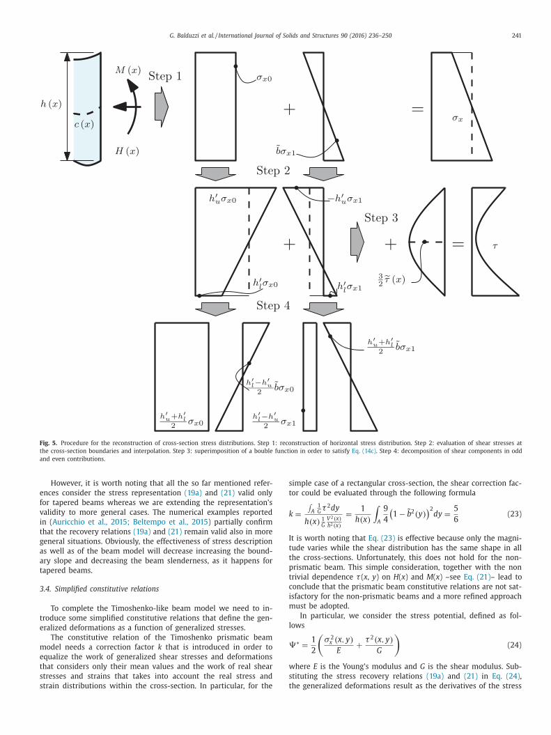
Therefore, we modify the recovery of cross-section shear-stress

distribution as illustrated in Fig. 5 . Specifically, given the general-

ized stresses H ( x ) and M ( x ) it is possible to reconstruct the hori-

zontal stress distribution within the cross-section and, in particu-

lar, to evaluate the horizontal stress magnitude on lower and upper

limits h l ( x ) and h u ( x ) (Step 1). Boundary equilibrium (8a) allows to

evaluate the shear stress at lower and upper limits of the cross-

section –τ | h l and τ | h u respectively– that thereafter we interpolate

through linear functions (Step 2). In order to satisfy Eq. (14c) we

add a bubble function to the linear shear stress distribution ob-

taining a parabolic shear stress distribution (Step 3). Finally, we

decompose the linear shear stress distributions in odd and even

contributions (Step 4).

Recalling the h l and h u definitions (2) and performing simple

calculations, the stress distributions result as follows

σx ( x, y ) = σx 0 ( x ) + ̃

b ( y ) · σx 1 ( x ) (19a)

τ ( x, y ) = c ′ ( x ) σx 0 ( x ) − h

′ (x )

2

σx 1 ( x )

+

(−h

′ (x )

2

σx 0 (x ) + c ′ (x ) σx 1 (x )

)˜ b (y )+

3

2 ̃

τ (x )(1− ˜ b 2 (y ))

(19b)

here the variables σ x 0 ( x ), σ x 1 ( x ), and

˜ τ ( x ) result defined as fol-

ows

x 0 ( x ) =

H ( x )

h ( x ) ; σx 1 ( x ) = M ( x )

6

h

2 ( x ) ;

˜ τ ( x ) =

(−V ( x )

h ( x ) − c ′ ( x ) σx 0 ( x ) +

h

′ ( x ) 2

σx 1 ( x )

)(20)

Finally, few algebraic steps allow us to express the shear stress

istribution as illustrated in the following

τ ( x, y ) =

(c ′ ( x ) σx 0 ( x ) − h

′ ( x ) 2

σx 1 ( x )

)(−1

2

+

3

2

˜ b 2 ( y )

)−

(h

′ ( x ) 2

σx 0 ( x ) − c ′ ( x ) σx 1 ( x )

)˜ b ( y ) +

3

2

τ0 ( x ) (1 −˜ b 2 ( y ) )

(21)

here the variable τ 0 ( x ) results defined as follows

0 ( x ) = −V ( x )

h ( x ) (22)

It is worth noting that the previously introduced quantities

ave a clear physical meaning:

• σ x 0 ( x ) is the mean value of the horizontal stress within the

cross-section,

• σ x 1 ( x ) is the maximum horizontal stress value induced by

bending moment that occurs at the cross-section lower limit,

and

• τ 0 ( x ) is the shear stress mean value.

In Eq. (21) , the shear distribution τ depends not only on V ( x ),

ut also on H ( x ) and M ( x ) that determine not only the magni-

ude but also the shape of the shear distribution. Finally, Eq. (21)

eads to conclude that the maximum shear stress does not occur in

orrespondence of the beam center-line, as noted by Paglietti and

arta (2007 , 2009 ).

The assumption of vanishing vertical stresses σy ( x, y ) = 0

grees with the assumptions of prismatic beam stress recovery,

ignificantly simplifying the beam model equations, but leads to vi-

late Eq. (8b) . Fortunately, this choice will not deeply worsen the

odel capability, as the numerical examples of Section 5 will il-

ustrate. On the other hand, readers may refer to ( Auricchio et al.,

015; Beltempo et al., 2015 ) for more refined models that do not

eglect the contribution of vertical stresses.

The recovery relation (21) is well known since the first half of

he twentieth century. In particular, referring to the analytical solu-

ion of the 2D equilibrium Eq. (5c) for an infinite long wedge, Atkin

1938) ; Cicala (1939) ; Timoshenko and Goodier (1951) express the

tress distribution as the combination of some trigonometric func-

ions. More in detail, Timoshenko and Goodier (1951) state that a

arabolic shear distribution is an approximation reasonably accu-

ate in the case of small boundary slope. Later on, Krahula (1975)

xtends the so far mentioned results to tapered beams, recover-

ng equations substantially identical to (19a) and (21) . Furthermore,

ore recently, Bruhns (2003 , Example 3.9) notes that (i) the shear

istribution in a tapered beam has no longer a distribution similar

o the prismatic beams, (ii) the shear distribution depends not only

n resulting shear, but also in bending moment and resulting hori-

ontal stress, and (iii) the maximum shear could occur everywhere

n the cross-section.

G. Balduzzi et al. / International Journal of Solids and Structures 90 (2016) 236–250 241

Fig. 5. Procedure for the reconstruction of cross-section stress distributions. Step 1: reconstruction of horizontal stress distribution. Step 2: evaluation of shear stresses at

the cross-section boundaries and interpolation. Step 3: superimposition of a bouble function in order to satisfy Eq. (14c) . Step 4: decomposition of shear components in odd

and even contributions.

e

f

v

i

t

g

a

a

t

3

t

e

m

e

t

s

s

s

t

k

I

t

t

p

t

c

i

m

l

�

w

s

t

However, it is worth noting that all the so far mentioned refer-

nces consider the stress representation (19a) and (21) valid only

or tapered beams whereas we are extending the representation’s

alidity to more general cases. The numerical examples reported

n ( Auricchio et al., 2015; Beltempo et al., 2015 ) partially confirm

hat the recovery relations (19a) and (21) remain valid also in more

eneral situations. Obviously, the effectiveness of stress description

s well as of the beam model will decrease increasing the bound-

ry slope and decreasing the beam slenderness, as it happens for

apered beams.

.4. Simplified constitutive relations

To complete the Timoshenko-like beam model we need to in-

roduce some simplified constitutive relations that define the gen-

ralized deformations as a function of generalized stresses.

The constitutive relation of the Timoshenko prismatic beam

odel needs a correction factor k that is introduced in order to

qualize the work of generalized shear stresses and deformations

hat considers only their mean values and the work of real shear

tresses and strains that takes into account the real stress and

train distributions within the cross-section. In particular, for the

imple case of a rectangular cross-section, the shear correction fac-

or could be evaluated through the following formula

=

∫ A

1 G τ 2 dy

h ( x ) 1 G V 2 ( x ) h 2 ( x )

=

1

h ( x )

∫ A

9

4

(1 − ˜ b 2 ( y )

)2 dy =

5

6

(23)

t is worth noting that Eq. (23) is effective because only the magni-

ude varies while the shear distribution has the same shape in all

he cross-sections. Unfortunately, this does not hold for the non-

rismatic beam. This simple consideration, together with the non

rivial dependence τ ( x , y ) on H ( x ) and M ( x ) –see Eq. (21) – lead to

onclude that the prismatic beam constitutive relations are not sat-

sfactory for the non-prismatic beams and a more refined approach

ust be adopted.

In particular, we consider the stress potential, defined as fol-

ows

∗ =

1

2

(σ 2

x ( x, y )

E +

τ 2 ( x, y )

G

)(24)

here E is the Young’s modulus and G is the shear modulus. Sub-

tituting the stress recovery relations (19a) and (21) in Eq. (24) ,

he generalized deformations result as the derivatives of the stress

242 G. Balduzzi et al. / International Journal of Solids and Structures 90 (2016) 236–250

t

a

a

o

o

b

P

m

V

f

(

t

a

m

t

b

4

e

S

i

e

c

4

s

potential with respect to the corresponding generalized stress.

Therefore we have

ε 0 ( x ) =

∫ A ( x )

∂�∗

∂H ( x ) dy = ε H H ( x ) + ε M

M ( x ) + ε V V ( x ) (25a)

χ( x ) =

∫ A ( x )

∂�∗

∂M ( x ) dy = χH H ( x ) + χM

M ( x ) + χV V ( x ) (25b)

γ ( x ) =

∫ A ( x )

∂�∗

∂V ( x ) dy = γH H ( x ) + γM

M ( x ) + γV V ( x ) (25c)

where

ε H =

(c ′ 2 ( x )

5 Gh ( x ) +

h

′ 2 ( x ) 12 Gh ( x )

+

1

Eh ( x )

)ε M

= χH = −8 c ′ ( x ) h

′ ( x ) 5 Gh

2 ( x ) ; ε V = γH =

c ′ ( x ) 5 Gh ( x )

χM

=

(9 h

′ 2 ( x ) 5 Gh

3 ( x ) +

12 c ′ 2 ( x ) Gh

3 ( x ) +

12

Eh

3 ( x )

)χV = γM

= − 3 h

′ ( x ) 5 Gh

2 ( x ) ; γV =

6

5 Gh ( x )

It is worth noting the following statements.

• Unlike the prismatic beam models, the generalized deforma-

tions depend on all generalized stresses.

• It is possible to recognize in ε H , χM

, and γ V the terms of pris-

matic beam constitutive laws

ε 0 ( x ) =

H ( x )

Eh ( x ) ; χ( x ) =

12 M ( x )

Eh

3 ( x ) ; γ ( x ) = − V ( x )

kGh ( x ) (26)

• The shear correction factor, as well as the other coefficients,

results naturally from the derivation procedure, bypassing the

problem of their evaluation.

To the author’s knowledge, Vu-Quoc and Léger (1992) are the

former researchers mentioning the non-trivial dependence of all

generalized deformations on all generalized stresses. Considering

the shear bending of a tapered beam, the authors derive the

beam’s flexibility matrix using the principle of complementary vir-

tual work. Later on, deriving a model for a tapered beam, Rubin

(1999) and Aminbaghai and Binder (2006) consider the fact that

the bending moment produces also shear deformation and the

shear force produces a curvature. Unfortunately, they do not con-

sider the effect of a non-horizontal center-line and Rubin (1999)

use different coefficients with respect to the ones reported in Eqs.

(25) , resulting energetically inconsistent. Conversely, for the model

derivation, Auricchio et al. (2015) ; Beltempo et al. (2015) ; Hodges

et al. (2008) use variational principles that have the advantage to

naturally derive the constitutive relations, but could lead to more

complicated equations, as already highlighted in Section 1 .

3.5. Remarks on beam model’s ODEs

In the following we resume the beam model’s ODEs according

to the notation adopted by Gimena et al. (2008a ). ⎧ ⎪ ⎪ ⎪ ⎪ ⎪ ⎪ ⎨ ⎪ ⎪ ⎪ ⎪ ⎪ ⎪ ⎩

H

′ (x )

V

′ (x )

M

′ (x )

ϕ

′ (x )

v ′ (x )

u

′ (x )

⎫ ⎪ ⎪ ⎪ ⎪ ⎪ ⎪ ⎬ ⎪ ⎪ ⎪ ⎪ ⎪ ⎪ ⎭

=

⎡ ⎢ ⎢ ⎢ ⎢ ⎢ ⎢ ⎣

0 0 0

0 0 0 0

0 0

−c ′ (x ) 1 0

χH χV χM

0 0 0

γH γV γM

1 0 0

ε H ε V ε M

−c ′ (x ) 0 0

⎤ ⎥ ⎥ ⎥ ⎥ ⎥ ⎥ ⎦

⎧ ⎪ ⎪ ⎪ ⎪ ⎪ ⎪ ⎨ ⎪ ⎪ ⎪ ⎪ ⎪ ⎪ ⎩

H(x )

V (x )

M(x )

ϕ(x )

v (x )

u (x )

⎫ ⎪ ⎪ ⎪ ⎪ ⎪ ⎪ ⎬ ⎪ ⎪ ⎪ ⎪ ⎪ ⎪ ⎭

−

⎧ ⎪ ⎪ ⎪ ⎪ ⎪ ⎪ ⎨ ⎪ ⎪ ⎪ ⎪ ⎪ ⎪ ⎩

q (x )

p(x )

m (x )

0

0

0

⎫⎪⎪⎪⎪⎪⎪⎬⎪⎪⎪⎪⎪⎪⎭(27)

With respect to Eq. (27) , it is worth noting what follows.

• The equations are naturally expressed as an explicit system of

first order ODEs.

• Similar to Gimena et al. (2008a ), the matrix that collects equa-

tions’ coefficients has a lower triangular form with vanishing

diagonal terms. As a consequence, the analytical solution can

easily be obtained through an iterative process of integration

done row by row, starting from H ( x ) and arriving at u ( x ).

• Reducing the beam model proposed by Gimena et al. (2008a )

to a 2D case, it is easy to recognize the same structure

in equilibrium and kinematics relations. Specifically Gimena

et al. (2008a ) use trigonometric coefficients whereas we

use the corresponding linearized ones (i.e., we assume that

sin ( θ ) � tan ( θ ) � θ ).

• The sub-matrix that collects the constitutive relation coeffi-

cients is symmetric with respect to the anti-diagonal.

• Finally, the sub-matrix that collects the constitutive relation

coefficients is completely full whereas Gimena et al. (2008a )

neglect coupling between curvature, horizontal, and vertical

resulting stresses (i.e., χH = χV = ε M

= γM

= 0 ). Examples re-

ported in Section 5 will illustrate that all the terms of the sim-

plified constitutive relations plays a crucial role and are in gen-

eral not negligible.

Now we move our attention back to the equilibrium (18) and

he compatibility (13) equations. It is worth noting that the use of

global Cartesian coordinate system presents the following main

dvantages.

• Both the beam equilibrium and compatibility are not influenced

by the cross-section size, which on the contrary plays a central

role in constitutive relations.

• Horizontal and vertical equilibrium are expressed through in-

dependent equations, whereas in classical formulation ( Bruhns,

2003 , Chapter 5) tangential and normal equilibrium equations

are coupled.

Furthermore, we note that few researchers follow the path

f using a global Cartesian coordinate system with cross-sections

rthogonal to x − axis. Fung and Kaplan (1952) investigate the

uckling of beams with small curvatures and Borri et al. (1992) ;

opescu et al. (20 0 0) ; Rajagopal and Hodges (2014) propose beam

odels considering oblique cross-sections. On the other hand,

ogel (1993) develops a second order Euler–Bernoulli beam model

or curved beams in large displacement regime and Gimena et al.

20 08b, 20 08a) develop 3D non-prismatic beam models expressing

he resulting forces in a global coordinate system.

Finally, if we neglect shear deformation in the proposed model

nd the second order terms in ( Vogel, 1993 ) –i.e., if we lead both

odels to use the same assumptions– we obtain the same equa-

ions, showing once more that the proposed model has the capa-

ility to recover simpler models available in literature.

. Tapered beam analytical solution

This section discusses the analytical solution of the ODEs gov-

rning the problem (27) for the simple case of a tapered beam.

pecifically, we consider a beam with an inclined center-line, as

llustrated in Fig. 6 .

The center-line and the thickness have the following analytical

xpressions

( x ) = c 1 x ; h ( x ) = h 1 x + h 0 (28)

.1. Homogeneous solution

Considering the geometry so far introduced, the homogeneous

olution of the beam model ODEs (27) is

G. Balduzzi et al. / International Journal of Solids and Structures 90 (2016) 236–250 243

Fig. 6. Tapered beam considered for the evaluation of the analytical solution: ge-

ometry and parameter’s definitions.

M

w

a

a

b

u

p

s

p

m

t

g

g

n

o

4

l

M

4

b

g

s

n

V

l

G

w

c

4

p

1

b

t

1

s

v

v

H ( x ) = C 6

( x ) = ( c 1 C 6 − C 5 ) x + C 4

V ( x ) = C 5

ϕ ( x ) = −3

(20 E c 2 1 + 3 E h

2 1 + 20 G

)10 EGh

2 1 h

2 ( x ) ( h 0 ( c 1 C 6 − C 5 ) − h 1 C 4 )

+

c 1 (60 E c 2 1 + E h

2 1 + 60 G

)5 EGh

2 1 h ( x )

C 6

−6

(10 E c 2 1 + E h

2 1 + 10 G

)5 EGh

2 1 h ( x )

C 5 + C 3

u ( x ) =

log ( h ( x ) )

60 EGh

3 1

(72 c 1 (10 E c 2 1 − E h

2 1 + 10 G

)( c 1 C 6 − C 5 )

+5 h

2 1 ( Eh 1 + 12 G ) C 6 + 12 c 1 Eh

2 1 C 5 )

−c 1

(60 E c 2 1 − 7 E h

2 1 + 60 G

)10 EGh

3 1 h ( x )

( h 0 ( C 5 − c 1 C 6 ) + h 1 C 4 )

+ c 1 xC 3 + C 2

v ( x ) = − log ( h ( x ) )

5 EGh

3 1

(c 1 (60 E c 2 1 − E h

2 1 + 60 G

)C 6

−3

(20 E c 2 1 + 3 E h

2 1 + 20 G

)C 5 )

−3

(20 E c 2 1 + E h

2 1 + 20 G

)10 EGh

3 1 h ( x )

( c 1 h 0 C 6 −h 0 C 5 −h 1 C 4 ) −xC 3 + C 1

(29)

here the parameters C 1 , C 2 , C 3 , C 4 , C 5 , and C 6 depend on bound-

ry conditions.

The analytical solution of non-prismatic beam (29) uses rational

nd logarithmic terms whereas the analytical solution of prismatic

eam uses polynomial terms. As a consequence, the polynomials

sually adopted in structural analysis in order to reconstruct the

rismatic beam displacement given the nodal displacements or as

hape functions for FE software, are no longer effective for non-

rismatic beams. Furthermore, the non-prismatic beam stiffness

atrix has a completely different structure that is influenced by

he non-trivial distribution of displacements along the beam lon-

itudinal axis and the strong coupling of all equations. The homo-

eneous solution (29) can be used to overcome these problems,

onetheless these aspects lie outside this paper’s aims and will be

bject of a further scientific paper.

.2. Particular solution

Considering a constant vertical load p ( x ) = p we obtain the fol-

owing particular solution for the beam model ODEs (27) .

H ( x ) = 0

( x ) =

1

2

px 2

V ( x ) = −px

ϕ ( x ) = − 3 p

20 EGh

3 1

(

2

(20 E c 2 1 + E h

2 1 + 20 G

)log ( h ( x ) )

−h

2 0

(20 E c 2 1 + 3 E h

2 1 + 20 G

)h

2 ( x )

+ 8

h 0

(10 E c 2 1 + E h

2 1 + 10 G

)h ( x )

)

u ( x ) = − 3 c 1 p

10 EGh

4 1

((20 E c 2 1 + E h

2 1 + 20 G

)h ( x ) ( log ( h ( x ) ) − 1 )

+

4

3

(60 E c 2 1 − E h

2 1 + 60 G

)h 0 log ( h ( x ) )

+

(20 E c 2 1 + E h

2 1 + 20 G

)h ( x ) +

h

2 0

(60 E c 2 1 − 7 E h

2 1 + 60 G

)6 h ( x )

+2 xEh

3 1

)v ( x ) =

3 p

EGh

4 1

((20 E c 2 1 + E h

2 1 + 20 G

)h ( x ) ( log ( h ( x ) ) − 1 )

+4 h 0

(20 E c 2 1 + 3 E h

2 1 + 20 G

)log ( h ( x ) )

+

1

2 h ( x )

(20 E c 2 1 + E h

2 1 + 20 G

)h

2 0 −

3 xEh

3 1

10

)(30)

.3. Asymptotic analysis

In this section, we perform some tests in order to evaluate ro-

ustness and correctness of the beam model. Specifically we are

oing to investigate two main aspects:

1. the behavior of the beam solution when the geometry tends to

become prismatic,

2. the capability of the beam model to recover the solution of a

tapered beam that has the straight axis rotated with respect to

the principal Cartesian coordinate system.

We consider a tapered cantilever, clamped in the initial cross-

ection and loaded with a vertical concentrated force in the fi-

al cross-section i.e., u ( 0 ) = ϕ ( 0 ) = v ( 0 ) = H ( l ) = M ( l ) = 0 , and

( l ) = 1 N . Furthermore, we assume the following values:

= 10 mm ; h ( 0 ) = αh ( l ) ; h ( l ) = 1 mm ; E = 10

5 MPa ; = 4 · 10

4 MPa (31)

here α is the ratio between the maximum and the minimum

ross-section sizes.

.3.1. Beam behavior for vanishing taper slope

To evaluate the non-prismatic beam behavior for vanishing ta-

er slope, we consider two cases:

1. a cantilever with an horizontal center-line i.e., c ( x ) = 0 where

all the cross-sections are symmetric with respect to the beam

longitudinal axis, denoted in the following as symm

2. a cantilever with an horizontal lower limit i.e., h l ( x ) = 0 and

c ( x ) = ( 1 − α) h ( l ) x 2 l , denoted in the following as unsym

We investigate the model behavior when the parameter α → i.e., when the beam becomes prismatic. Since it is not possi-

le to evaluate analytically the displacement limit, we evaluate

he maximum vertical displacement v ( l ) varying α between 2 and

+ 1 · 10 −9 mm .

The maximum vertical displacement for the Timoshenko beam

olution, indicated in the following as v as assume the following

alue:

as =

1

3

V ( l ) l 3

E h 3

12

+

6

5

V ( l ) l

Gh

= 0 . 0403 mm (32)

244 G. Balduzzi et al. / International Journal of Solids and Structures 90 (2016) 236–250

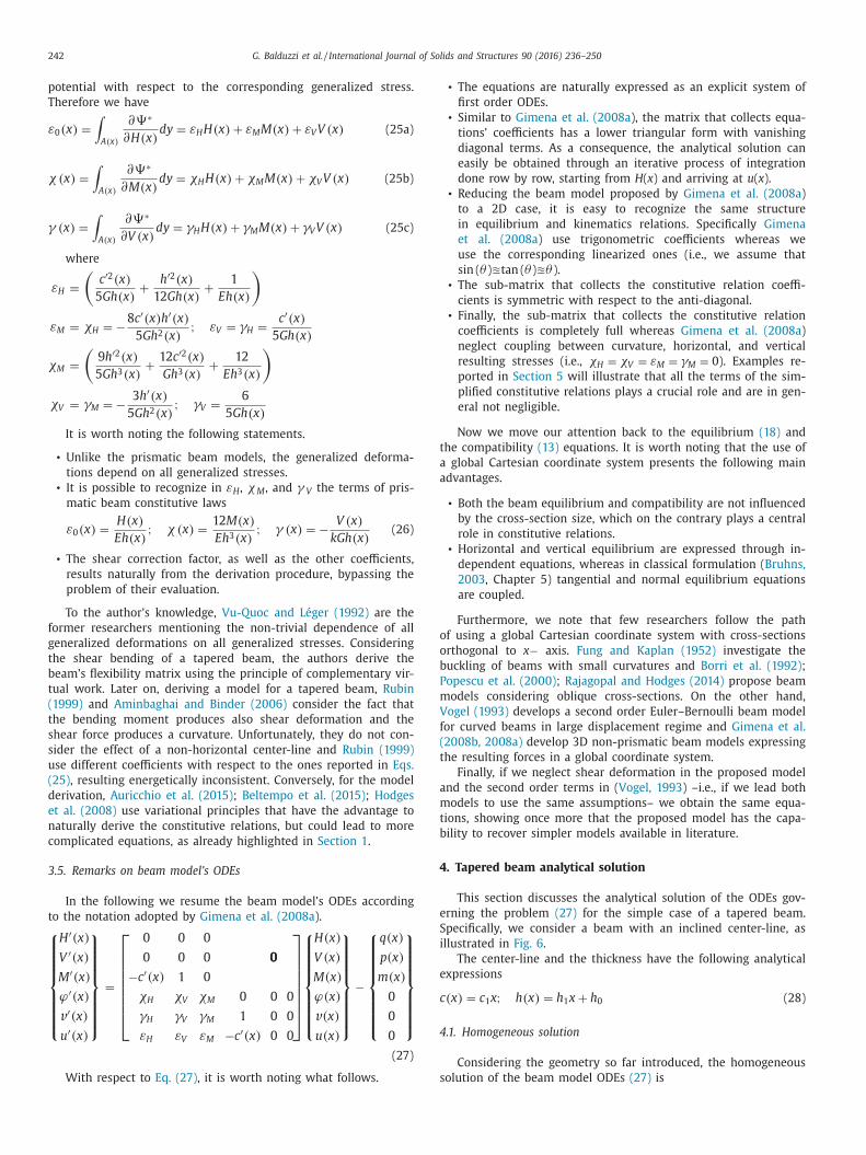
Fig. 7. Asymptotic behavior of a tapered cantilever loaded with a shear force V ( l ) = 1 N applied in the final cross-section.

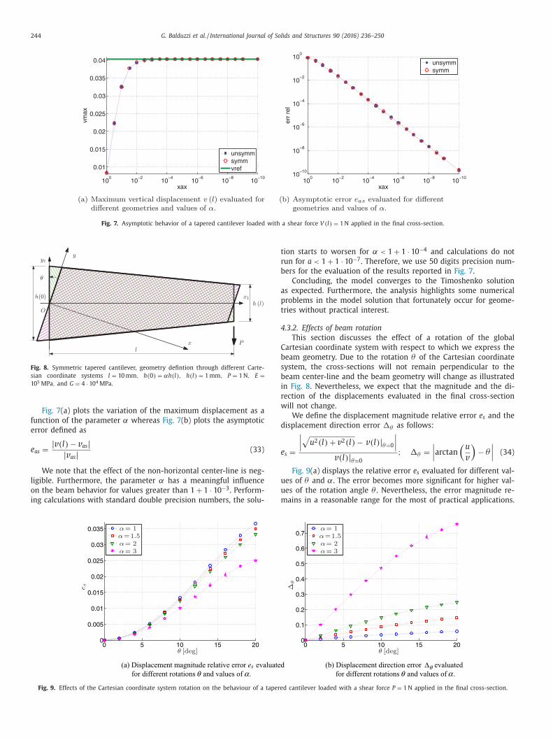
Fig. 8. Symmetric tapered cantilever, geometry defintion through different Carte-

sian coordinate systems l = 10 mm , h ( 0 ) = αh ( l ) , h ( l ) = 1 mm , P = 1 N , E =

10 5 MPa , and G = 4 · 10 4 MPa .

t

r

b

a

p

t

4

C

b

s

b

i

r

w

d

e

u

u

m

Fig. 7 (a) plots the variation of the maximum displacement as a

function of the parameter α whereas Fig. 7 (b) plots the asymptotic

error defined as

e as =

| v ( l ) − v as | | v as | (33)

We note that the effect of the non-horizontal center-line is neg-

ligible. Furthermore, the parameter α has a meaningful influence

on the beam behavior for values greater than 1 + 1 · 10 −3 . Perform-

ing calculations with standard double precision numbers, the solu-

Fig. 9. Effects of the Cartesian coordinate system rotation on the behaviour of a tapere

ion starts to worsen for α < 1 + 1 · 10 −4 and calculations do not

un for a < 1 + 1 · 10 −7 . Therefore, we use 50 digits precision num-

ers for the evaluation of the results reported in Fig. 7 .

Concluding, the model converges to the Timoshenko solution

s expected. Furthermore, the analysis highlights some numerical

roblems in the model solution that fortunately occur for geome-

ries without practical interest.

.3.2. Effects of beam rotation

This section discusses the effect of a rotation of the global

artesian coordinate system with respect to which we express the

eam geometry. Due to the rotation θ of the Cartesian coordinate

ystem, the cross-sections will not remain perpendicular to the

eam center-line and the beam geometry will change as illustrated

n Fig. 8 . Nevertheless, we expect that the magnitude and the di-

ection of the displacements evaluated in the final cross-section

ill not change.

We define the displacement magnitude relative error e s and the

isplacement direction error �θ as follows:

s =

∣∣∣√

u

2 ( l ) + v 2 ( l ) − v ( l ) | θ=0

∣∣∣v ( l ) | θ=0

; �θ =

∣∣∣arctan

(u

v

)− θ

∣∣∣ (34)

Fig. 9 (a) displays the relative error e s evaluated for different val-

es of θ and α. The error becomes more significant for higher val-

es of the rotation angle θ . Nevertheless, the error magnitude re-

ains in a reasonable range for the most of practical applications.

d cantilever loaded with a shear force P = 1 N applied in the final cross-section.

G. Balduzzi et al. / International Journal of Solids and Structures 90 (2016) 236–250 245

Fig. 10. Double-tapered beam under constant and distributed vertical load p .

F

v

i

c

4

c

t

d

t

v

v

n

a

ϕ

(

s

k

a

b

e

k

(

T

a

a

d

s

o

m

F

e

t

l

c

t

i

w

o

5

t

p

a

fi

5

(

1

b

t

g

H

ig. 9 (b) displays the displacement direction error �θ for different

alues of θ and α. The results are reasonably accurate in predict-

ng the right direction of displacement, at least in the considered

ases.

.4. Maximum displacement for symmetric, double-tapered beams

This section considers the double tapered beam loaded with a

onstant vertical load depicted in Fig. 10 . In particular, this geome-

ry is of interest since it is often used to shape beams that support

ouble pitched roofs.

According to several results reported in literature, we express

he beam maximum displacement v max as the sum of the bending

E and the shear v G contributions as follows:

max = v E + v G = − 5

384

k E 12

h

3 0 b

pl 4

E − 1

8

k G 6

5

pl 2

Gh 0 b (35)

Exploiting the beam symmetry, using both the homoge-

eous (29) and the particular (30) solutions, and imposing suit-

ble boundary values (i.e., u ( 0 ) = v ( 0 ) = M ( 0 ) = H ( l/ 2 ) = V ( l/ 2 ) = ( l/ 2 ) = 0 ) the coefficients k E and k G results defined as follows

k E = −6

5

8 α3 − 11 α2 + 4 α − 1 − 2 α2 log ( α) ( 2 α + 1 )

α2 ( α − 1 ) 4

k G = −1

2

29 α3 − 40 α2 + 15 α − 4 − 2 α2 log ( α) ( 8 α + 3 )

α2 ( α − 1 ) 2

(36)

On the other hand, considering the model proposed by Rubin

1999) , Schneider and Albert (2014) proposes the following expres-

ions for the coefficients k E and k G :

E =

1

α3 (0 . 15 +

0 . 85 α

) ; k G =

2

1 + α2 / 3 (37)

Finally, considering the Timoshenko prismatic beam equations,

ssuming only that cross-section area and inertia vary along the

eam axis, Ozelton and Baird (2002) proposed the following

Fig. 11. Coefficients k E and k G for the evaluation of the maxi

xpressions for the coefficients k E and k G :

k E =

19 . 2

( α − 1 ) 3

(2

α + 2

α − 1

log

(α + 1

2

)+

3

α + 1

− 2

( α + 1 ) 2

− 4

) G =

4

α − 1

(α + 1

α − 1

log

(α + 1

2

)− 1

)(38)

Fig. 11 reports the coefficients evaluated according to Eqs. (36) ,–

38) .

All the functions reported in Fig. 11 converge to 1 for α → 1.

his is an expected behavior since if α = 1 we are considering

prismatic beam and therefore no correction factors must be

pplied to Eq. (35) in order to evaluate the beam maximum

isplacement. Fig. 11 (a) highlights that Eqs. (36) and (37) provide

ubstantially identical evaluation of the coefficient k E . On the

ther hand, with respect to the proposed model, Eq. (38) overesti-

ates the bending contribution of values that could exceed 100%.

ig. 11 (b) highlights that each model provides completely different

valuations of the coefficient k G . Furthermore, with respect to

he model derived in this paper, both the formulas proposed in

iterature underestimates the shear contribution of values that

ould exceed the 40%.

The adoption of Eqs. (36) in engineering practice needs addi-

ional considerations on material constitutive law and rigorous val-

dations that lie outside this paper’s aims. This specific aspect, as

ell as of other aspects of interest for practitioners, will be object

f a further scientific paper.

. Numerical examples

This section aims at providing further details about the ob-

ained model capabilities. We consider two examples: (i) a ta-

ered cantilever and (ii) an arch shaped beam. Both cases were

lready analyzed in ( Auricchio et al., 2015 ) considering a more re-

ned model.

.1. Tapered beam

We consider the symmetric tapered beam illustrated in Fig. 12

l = 10 mm , h ( 0 ) = 1 mm , and h ( l ) = 0 . 5 mm ) and we assume E =0 5 MPa and G = 4 · 10 4 MPa as material parameters. Moreover, the

eam is clamped in the initial cross-section A (0) and a concen-

rated load P P P = [ 0 , −1 ] N acts on the final cross-section A ( l ).

Solving Eqs. (18) , we obtain the following expressions for the

eneralized stresses

( x ) = 0 ; M ( x ) = x − 10 ; V ( x ) = 1 (39)

mum displacement, evaluated with different methods.

246 G. Balduzzi et al. / International Journal of Solids and Structures 90 (2016) 236–250

Fig. 12. Symmetric tapered beam: l = 10 mm , h ( 0 ) = 1 mm , h ( l ) = 0 . 5 mm , P =

1 N , E = 10 5 MPa , and G = 4 · 10 4 MPa .

F

c

t

c

A

i

a

e

t

m

o

Fig. 13. Horizontal (a)) and shear (b) stresses cross-section distributions, computed in th

applied in the final cross-section.

Fig. 14. Curvature (a), and shear deformation (b) axial distributions, evaluated for a

Fig. 15. Rotation (a) and vertical displacements (b) axial distributions, evaluated for a

ig. 13 depicts the distributions of the stresses σ x and τ in the

ross-section A (0.5 l ). The label mod indicates the stress distribu-

ion obtained using Eqs. (19a) and (21) , whereas the label ref indi-

ates the 2D FE solution, computed using the commercial software

BAQUS ( Simulia, 2011 ), considering the full 2D problem, and us-

ng a structured mesh of 7680 × 512 bilinear elements. Fig. 13 (b)

llows to appreciate a difference between the model and the refer-

nce solution, nevertheless the relative error magnitude is smaller

han 1 · 10 −3 .

Since H ( x ) = 0 therefore ε H H ( x ) = χH H ( x ) = γH H ( x ) = 0 ;

oreover, since c ( x ) = 0 also ε M

= ε V = 0 . Fig. 14 depicts the plots

f the generalized deformations χ ( x ) and γ ( x ). The curvature

e cross-section A (0.5 l ) for a symmetric tapered beam with a vertical load P = 1 N

tapered cantilever with a shear load P = 1 N applied in the final cross-section.

tapered cantilever with a shear load P = 1 N applied in the final cross-section.

G. Balduzzi et al. / International Journal of Solids and Structures 90 (2016) 236–250 247

Fig. 16. Arch shaped beam: l = 10 mm , � = 0 . 5 mm , h ( l ) = h ( 0 ) = 0 . 6 mm , q =

1 N / mm , E = 10 5 MPa , and G = 4 · 10 4 MPa .

i

r

χ

γ

a

r

f

a

(

–

Fig. 17. Horizontal (a) and shear (b) stresses cross-section distributions, computed in the

applied in the final cross-section.

Fig. 18. Horizontal (a), curvature (c), shear (d) deformations, and horizontal elongation in

shaped beam with an horizontal load Q = 0 . 6 N applied in the final cross-section.

nduced by vertical forces χV V ( x ) has a negligible magnitude with

espect to the curvature induced by resulting bending moment

M

M ( x ). On the other hand both shear deformations γ M

M ( x ) and

V V ( x ) have the same order of magnitude and therefore both play

crucial role in determining the tapered beam’s behavior.

Fig. 15 reports the beam displacements ϕ( x ) and v ( x ) . Table 1

eports the maximum vertical displacement evaluated with dif-

erent models (i.e., the model proposed in this paper –indicated

s Analytical model–, the model developed by Auricchio et al.

2015) –indicated as ABL–, and the FE analysis software ABAQUS

indicated as v re f –). We note that all the models are accurate

cross-section A (0.75 l ) for an arch shaped beam with an horizontal load Q = 0 . 6 N

duced by inclined center-line rotation (b) axial distributions evaluated for an arch

248 G. Balduzzi et al. / International Journal of Solids and Structures 90 (2016) 236–250

Table 1

Mean value of the vertical displacement evaluated on the final cross-section and

obtained considering different models for a symmetric tapered cantilever with a

vertical load P = 1 N applied in the final cross-section.

Beam model v ( 10 ) mm

| v −v re f | | v re f |

Analytical model −0.0657826 1 . 064 · 10 −3

ABL −0.0657294 2 . 541 · 10 −4

2D solution ( v re f ) −0.0657127 –

g

H

a

i

A

u

t

W

t

0

χ

m

m

t

i

m

m

d

γ

l

t

d

in predicting vertical displacement. Because it is more refined,

ABL provides the most accurate prediction of vertical displacement

whereas, being less refined, the analytical model proposed in this

paper is the less accurate. However, the analytical model shows a

good accuracy, acceptable in most engineering applications.

5.2. Arch shaped beam

We now consider the arch shaped beam depicted in Fig. 16 . The

beam center-line and cross-section height are defined as

c ( x ) := − 1

100

x 2 +

1

10

x ; h ( x ) :=

1

50

x 2 − 1

5

x +

3

5

(40)

Moreover, the beam is clamped in the initial cross-section A (0) and

loaded on the final cross-section A ( l ) with a constant horizontal

load distribution t t t | A ( l ) = [ 1 , 0 , 0 ] T N / mm .

Fig. 19. Horizontal (a) and vertical (c) displacements and rotation (b) evaluated for an arc

Solving Eqs. (18) , we obtain the following expressions for the

eneralized stresses

( x ) =

3

5

; M ( x ) =

3

5

·(− 1

100

x 2 +

1

10

x

); V ( x ) = 0 (41)

Fig. 17 depicts the cross-section distributions of the stresses σ x

nd τ . The label mod indicates the stress distribution obtained us-

ng Eqs. (19a) and (21) , whereas the label ref indicates the 2D

BAQUS solution, computed considering the full 2D problem and

sing a structured mesh of 10240 × 256 bilinear elements. In order

o exclude boundary effects, we consider the cross-section A (0.75 l ).

e note the good agreement between the Analytical model and

he 2D FE solution.

Since V ( x ) = 0 therefore we have ε V V ( x ) = χV V ( x ) = γV V ( x ) = . Fig. 18 (a), (c), and (d) depict the generalized deformation ε 0 ( x ),( x ), and γ ( x ) , respectively. We note that the horizontal defor-

ation induced by the bending moment ε M

M ( x ) has negligible

agnitude compared with the horizontal deformation induced by

he resulting horizontal stress ε H H ( x ). Analogously, the curvature

nduced by resulting horizontal stress χH H ( x ) has a negligible

agnitude with respect to the curvature induced by bending mo-

ent χM

M ( x ). On the other hand, both the shear deformations in-

uced by resulting horizontal stress γ H H ( x ) and bending moment

M

M ( x ) have non-vanishing magnitudes.

Fig. 18 (b) shows the horizontal elongation induced by center-

ine rotation c ′ ( x ) ϕ. This quantity is two order of magnitude bigger

han the horizontal deformation ε 0 ( x ), and plays a central role in

etermining the horizontal displacements u .

Fig. 19 reports the beam displacements u ( x ), ϕ( x ), and v ( x ) .

h shaped beam with an horizontal load Q = 0 . 6 N applied in the final cross-section.

G. Balduzzi et al. / International Journal of Solids and Structures 90 (2016) 236–250 249

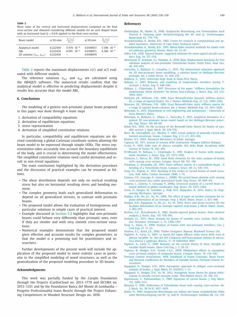
Table 2

Mean value of the vertical and horizontal displacements computed on the final

cross-section and obtained considering different models for an arch shaped beam

with an horizontal load Q = 0 . 6 N applied in the final cross-section.

Beam model v ( 10 ) mm

| v −v re f | | v re f | u (10) mm

| u −u re f | | u re f |

Analytical model 0.222569 5 . 979 · 10 −4 0.0109037 5 . 598 · 10 −4

ABL 0.222434 8 . 991 · 10 −6 0.0108971 4 . 588 · 10 −5

2D solution ( v re f , u re f ) 0.222436 – 0.0108976 –

u

t

a

r

6

i

r

b

r

o

T

s

a

l

p

u

g

A

t

2

P

i

R

A

A

A

A

A

A

BB

B

B

B

B

B

B

B

BC

C

E

F

F

F

G

G

G

H

H

K

K

O

O

P

P

P

P

R

R

R

R

R

Table 2 reports the maximum displacements v ( l ) and u ( l ) eval-

ated with different models.

The reference solutions v re f and u ref are calculated using

he ABAQUS software. The numerical results confirm that the

nalytical model is effective in predicting displacements despite it

esults less accurate than the model ABL.

. Conclusions

The modeling of a generic non-prismatic planar beam proposed

n this paper was done through 4 main steps

1. derivation of compatibility equations

2. derivation of equilibrium equations

3. stress representation

4. derivation of simplified constitutive relations

In particular, compatibility and equilibrium equations are de-

ived considering a global Cartesian coordinate system allowing the

eam model to be expressed through simple ODEs. The stress rep-

esentation takes accurately into account the boundary equilibrium

f the body, and is crucial in determining the model effectiveness.

he simplified constitutive relations need careful derivation and re-

ult in non-trivial equations.

The main conclusions highlighted by the derivation procedure

nd the discussion of practical examples can be resumed as fol-

ows.

• The shear distribution depends not only on vertical resulting

stress but also on horizontal resulting stress and bending mo-

ment.

• The complex geometry leads each generalized deformation to

depend on all generalized stresses, in contrast with prismatic

beams.

• The proposed model allows the evaluation of homogeneous and

particular solutions in simple cases of practical interest.

• Example discussed in Section 5.2 highlights that non-prismatic

beams could behave very differently than prismatic ones, even

if they are slender and with very smooth cross-section varia-

tions.

• Numerical examples demonstrate that the proposed model

gives effective and accurate results for complex geometries, so

that the model is a promising tool for practitioners and re-

searchers.

Further developments of the present work will include the ap-

lication of the proposed model to more realistic cases in partic-

lar to the simplified modeling of wood structures, as well as the

eneralization of the proposed modeling procedure to 3D beams.

cknowledgments

This work was partially funded by the Cariplo Foundation

hrough the Projects iCardioCloud no. 2013–1779 and SICURA no.

013–1351 and by the Foundation Banca del Monte di Lombardia –

rogetto Professionalitá Ivano Benchi through the Project Enhanc-

ng Competences in Wooden Structure Design no. 1056.

eferences

minbaghai, M. , Binder, R. , 2006. Analytische Berechnung von Voutenstäben nach

Theorie II. Ordnung unter Berücksichtigung der M- und Q- Verformungen.

Bautechnik 83, 770–776 . runakirinathar, K. , Reddy, B.D. , 1992. Centre for research in computational and ap-

plied mechanics, University of Cape Town Technical report . runakirinathar, K. , Reddy, B.D. , 1993. Mixed finite element methods for elastic rods

orf arbitrary geometry. Numer. Math. 64, 13–43 . tkin, E.H. , 1938. Tapered beams: suggested solutions for some typical aircraft cases.

Aircr. Eng. 10, 371–374 .

ttarnejad, R. , Semnani, S.J. , Shahaba, A. , 2010. Basic displacement functions for freevibration analysis of non-prismatic Timoshenko beams. Finite Elem. Anal. Des.

46, 916–929 . uricchio, F. , Balduzzi, G. , Lovadina, C. , 2015. The dimensional reduction approach

for 2D non-prismatic beam modelling: a solution based on Hellinger-Reissnerprinciple. Int. J. Solids Struct. 15, 264–276 .

alduzzi, G. , 2013. Univeristà degli Studi di Pavia Ph.d. thesis . alkaya, C. , 2001. Behavior and modeling of nonprismatic members having T-

sections. J. Struct. Eng. 8, 940–946 .

alkaya, C. , Citipitioglu, E. , 1997. Discusson of the paper “stiffness formulation fornonprismatic beam elements” by Arture Tena-Colunga. J. Struct. Eng. 123 (12),

1694–1695 . anerjee, J.R. , Williams, F.W. , 1985. Exact Bernoulli-Euler dynamic stiffness matrix

for a range of tapered beams. Int. J. Numer. Methods Eng. 21 (12), 2289–2302 . anerjee, J.R. , Williams, F.W. , 1986. Exact Bernoulli-Euler static stiffness matrix for

a range of tapered beam-columns. Int. J. Numer. Methods Eng. 23, 1615–1628 .

eltempo, A. , 2013. Department of civil engineering and architecture – University ofPavia Master’s thesis .

eltempo, A. , Balduzzi, G. , Alfano, G. , Auricchio, F. , 2015. Analytical derivation of ageneral 2D non-prismatic beam model based on the Hellinger-Reissner princi-

ple. Eng. Struct. 101, 88–98 . oley, B.A. , 1963. On the accuracy of the Bernoulli-Euler theory for beams of vari-

able section. J. Appl. Mech. 30, 374–378 .

orri, M. , Ghiringhelli, G.L. , Merlini, T. , 1992. Linear analysis of naturally curved andtwisted anisotropic beams. Compos. Eng. 2 (5–s7), 433–456 .

ruhns, O.T. , 2003. Advanced Mechanics of Solids. Springer . apurso, M. , 1971. Lezioni di Scienza delle Costruzioni. Pitagora Editrice Bologna .

icala, P. , 1939. Sulle travi di altezza variabile. Atti della Reale Accademia delleScienze di Torino 74, 392–402 .

l-Mezaini, N. , Balkaya, C. , Citipitioglu, E. , 1991. Analysis of frames with nonpris-

matic members. J. Struct. Eng. 117, 1573–1592 . ranciosi, C. , Mecca, M. , 1998. Some finite elements for the static analysis of beams

with varying cross section. Comput. Struct. 69, 191–196 . riedman, Z. , Kosmatka, J.B. , 1993. Exact stiffness matrix of a nonuniform beam - II

bending of a Timoshenko beam. Comput.s Struct. 49 (3), 545–555 . ung, Y.C. , Kaplan, A. , 1952. Buckling of low arches or curved beams of small curva-

ture. Natl. Advis. Comm. Aeronaut. 2840, 1–75 .

imena, F.N. , Gonzaga, P. , Gimena, L. , 2008b. 3D-curved beam element with varyingcross-sectional area under generalized loads. Eng. Struct. 30, 404–411 .

imena, L. , Gimena, F. , Gonzaga, P. , 2008a. Structural analysis of a curved beam el-ement defined in global coordinates. Eng. Struct. 30, 3355–3364 .

ross, D. , Hauger, W. , Schröder, J. , Wall, W.A. , Rajapakse, N. , 2012. Statics. In: Engi-neering Mechanics. Springer .

odges, D.H. , Ho, J.C. , Yu, W. , 2008. The effect of taper on section constants for in-

plane deformation of an isotropic strip. J. Mech. Mater. Struct. 3, 425–440 . odges, D.H. , Rajagopal, A. , Ho, J.C. , Yu, W. , 2010. Stress and strain recovery for the

in-plane deformation of an isotropic tapered strip-beam. J. Mech. Mater. Struct.5, 963–975 .

echter, G.E. , M.Gutkowski, R. , 1984. Double-tapered glulam beams: finite elementanalysis. J. Struct. Eng. 110, 978–991 .

rahula, J.L. , 1975. Shear formula for beams of variable cross section. AIAA (Am.Inst. Aeronaut. Astronaut.) J. 13, 1390–1391 .

zay, G. , Topcu, A. , 20 0 0. Analysis of frames with non-prismatic members. Can. J.

Civil Eng. 27, 17–25 . zelton, E.C. , Baird, J.A. , 2002. Timber Designers’ Manual. Blackwell Science Ltd .

aglietti, A. , Carta, G. , 2007. La favola del taglio efficace nella teoria delle travi dialtezza variabile. In: Atti del XVI Congresso dell’Associazione italiana di mecca-

nica teorica e applicata, Brescia, 11–14 Settembre 2007 . aglietti, A. , Carta, G. , 2009. Remarks on the current theory of shear strength of

variable depth beams. Open Civil Eng. J. 3, 28–33 .

opescu, B. , Hodges, D.H. , Cesnik, C.E.S. , 20 0 0. Obliqueness effects in asymptoticcross-sectional analysis of composite beams. Comput. Struct. 76, 533–543 .

ortland Cement Associations , 1958. Handbook of Frame Constants. Beam Factorand Moment Coefficients for Members of Variable Section. Portland Cement As-

sociations . ajagopal, A. , Hodges, D.H. , 2014. Asymptotic approach to oblique cross-sectional

analysis of beams. J. Appl. Mech. 81 (031015), 1–15 .

ajagopal, A. , Hodges, D.H. , Yu, W. , 2012. Asymptotic beam theory for planar defor-mation of initially curved isotropic strips. Thin-Walled Struct. 50, 106–115 .

ajasekaran, S. , Padmanabhan, S. , 1989. Equations of curved beams. J. Eng. Mech.115, 1094–1111 .

omano, F. , 1996. Deflections of Timoshenko beam with varying cross-section. Int.J. Mech. Sci. 38 (8-9), 1017–1035 .

ubin, H. , 1999. Analytische Berechnung von Stäben mit linear veränderlicher Höhe

unter Berücksichtigung von M-, Q- und N- Verformungen. Stahlbau 68, 112–119 .

250 G. Balduzzi et al. / International Journal of Solids and Structures 90 (2016) 236–250

T

T

V

Y

Sapountzakis, E.J. , Panagos, D.G. , 2008. Shear deformation effect in non-linear anal-ysis of composite beams of variable cross section. Int. J. Non-Linear Mech. 43,

660–682 . Schneider, K. , Albert, A. , 2014. Bautabellen für Ingenieure: mit Berechnungshin-

weisen und Beispielen. Bundesanzeiger Verlag GmbH . Shooshtari, A. , Khajavi, R. , 2010. An efficent procedure to find shape functions and

stiffness matrices of nonprismatic Euler-Bernoulli and Timoshenko beam ele-ments. Eur. J. Mech., A/Solids 29, 826–836 .

Simulia , 2011. ABAQUS User’s and Theory Manuals - Release 6.11. Simulia, Provi-

dence, RI, USA . Tena-Colunga, A. , 1996. Stiffness formulation for nonprismatic beam elements. J.

Struct. Eng. 122, 1484–1489 .

imoshenko, S. , 1955. Elementary theory and problems. In: Strength of materials.Krieger publishing company .

imoshenko, S. , Goodier, J.N. , 1951. Theory of Elasticity, second ed. McGraw-Hill . Timoshenko, S.P. , Young, D.H. , 1965. Theory of Structures. McGraw-Hill .

Vogel, U. , 1993. Berechnung von Bogentragwerken nach del Elastizitätstheorie II:Ordnung. chapter 3.5 in stahlbau handbuch für studium und praxis band 1, teil

a. Stahlbau-Verlagsgesellschaft mbH Köln 1, 211–226 . u-Quoc, L. , Léger, P. , 1992. Efficient evaluation of the flexibility of tapered I-beams

accounting for shear deformations. Int. J. Numer. Methods Eng. 33 (3), 553–566 .

u, W. , Hodges, D.H. , Volovoi, V. , Cesnik, C.E. , 2002. On Timoshenko-like modelingof initially curved and twisted composite beams. Int. J. Solids Struct. 39, 5101–

5121 .