international journal of advance research, ijoar fileeoq model is that all units purchased or...

INTERNATIONAL JOURNAL OF ADVANCE RESEARCH, IJOAR .ORG ISSN 2320-9143 1

IJOAR© 2014 http://www.ijoar.org

International Journal of Advance Research, IJOAR .org

Volume 2, Issue 7, July 2014, Online: ISSN 2320-9143

AN ENTROPIC PRODUCTION OR ORDER QUANTITY

MODEL WITH IMPERFECT QUALITY WITH PRICE SENSITIVE

DEMAND Dr Sudipta Sinha Department of Mathematics Burdwan Raj College,University of Burdwan,West Bengal,Pin-713104 Email: [email protected]

Abstract:-

This paper deals with an entropic order quantity (EnOQ) model over a finite time. The

model hypothesizes production inventory situation where items received or produced are

not of good quality. Items of imperfect quality, not necessarily defective, could be used in

another production inventory situation i.e. less restrictive process and acceptance control.

This paper considers the issue that poor-quality items are sold as a single batch by the end

of the 100% screening process. The demand depends on the selling price. At the end a

numerical is set to illustrate the results obtained and sensitivity analysis of various

parameters is carried out.

Keywords:-

ENOQ, Imperfect quality, Price-sensitive demand, Screening, Entropy.



1. Introduction:-

Ever since the EOQ model was introduced in the earliest decades of this century, it

appears that it is still widely accepted by many industries today. However, the

assumptions of the EOQ model are widely met. This has led many researchers to study

the EOQ extensively under real- life situations. A common unrealistic assumption of the

EOQ model is that all units purchased or produced are of good quality. It is very difficult

to produce or purchase items with 100% good quality .Hence the issue of inventory

model with imperfect quality has received considerable attention by researchers.

employed the renewal process theorem to rectify a flaw in an EOQ model with unreliable

supply, characterized by a random fraction of imperfect quality items and a screening

process developed Salemah et al[24]. The works of Eroglu et al [9] and Maddah et al [16]

are based on thex

D1ρ assumption.However; Papachristos et al [17] questioned the

validity of the assumption, but failed to provide a correction to this defect. Rosenblatt et

al [21] assumed that the defectives items could be reworked instantaneously at a cost and

found that the presence of defective items motivates smaller lotsizes.At the same time,

Porteus [20] developed a simple model that captures a significant relationship between

quality and lot-size and observed similar results. Both of the above models implicitly

assumed the defective items could not be salvaged.Salemeh et al [24] unlike the

assumption of Rosenblatt et al [21] assumed that poor-quality items are sold as a single

batch by the end of 100% screening process and found that the economic lot-size quantity

tended to increase as the average percentage of imperfect quality items increased. Roy et

al [22] also proposed an EOQ model where all the items are not good quality.Jaber et al

[12] assumed the defective items per lot according to a learning curve,which was

empirically validated by data from the automotive industry They found that the

inspection rate was much higher than the demand rate and with learning effects and the

percentage defectives per shipment reduce to a small value.Lin [15] determined optimal

strategy for supply chain system where some items are defective. Wee et al [30]

employed the unscreened items from the received lot to replace the defective items.Yoo

et al [29] proposed a profit maximization imperfect quality inventory model with two

types of inspection errors(TypeI and II) and defective sales return that determines an

optimal production lot size.

Related to the task is the paper by Cardenas-Barron [5] where an error appearing on and

Salemeh et al‟s[24] work was corrected. Thereafter with respect to the inventory model

proposed by Salemeh et al [24] ,Chung [7] fuzzified the defective rate and the annual

demand and then derived the corresponding optimal lot sizes.Zhang et al [31] considered

a joint lot-sizing and inspection policy with random yield where defective units cannot be

used and thus must be replaced by non-defective ones. But none of them considered

price-sensitive demand; all of them considered the constant demand.Chung et al [8]

developed an EOQ model to determine retailer‟s optimal cycle time with imperfect

quality items considering permissible delay in payments.

Generally reduction of selling price increases the demand. Price discount motivates the

retailers to order more quantities of items since demands of customers are

increased.Therefore,overall profit is increased due to more demand.EOQ models with

price sensitive demand are developed by Bernstein[3],Burewell [4],Sana,S.S.[25],Teng

et al[26].Kar et al [13] focused on multi-item inventory model with price-dependent

demand and imprecise goal. Optimal credit policy to increase supplier‟s profit when



demand is price dependent is determined by Kim et al [14].Yang et al [28] provided a

model to determine optimal lot size using quantity discount when demand is price

sensitive.

Abad[1,2] determined optimal pricing and economic order quantity under the partial

backlogging, shortages etc.Chang et al[6] also determined retailer‟s optimal selling price

and lot-size for deteriorating items.Sabahno,H[23] derived an optimal policy for

deteriorating inventory model where demand depends on price.

Inclusion of entropy cost now becomes an important feature in developing EOQ model.

Jaber et al [10] proposed an analogy between the behavior of production system and the

behavior of physical system. Before that Jaber[11] derived an inventory model with

permissible delay in payments including entropy cost. In this paper entropy cost has been

included. Entropy is generally defined as the account of disorder in a system. The need

for an entropy cost of the cycle time is a key feature of specific perishable products like

fruits, vegetables, food stuffs, fishes etc.The use of entropy must carefully be

planned,taking into account the multiplicity of objectives inherent in this kind of decision

problem. M.Pattnaik [18] introduced the concept of entropy cost to account for hidden

cost such as the additional managerial cost which is essential smooth running of a

business sector.Pattnaik [19] proposed a non-linear profit maximization entropic order

quantity (EnOQ) model for deteriorating items with two component demand rate. Before

that model Pattnaik [19] also developed two models on EnOQ one of which is instant

deterioration of perishable items with price discounts and another is post deterioration

cash discounts.An EnOQ model with fuzzy holding cost and fuzzy disposal cost is

suggested by Tripathy et al[27].In this model they consider two-component demand and

discounted selling ptice.

In this paper an Entropic order quantity model is proposed when all the items received

are not of good quality and demand is price sensitive. A 100% screening is performed

and a numerical example is provided in support of the proposed model. Optimal order

quantity and optimal selling price of the example are determined using the Software of

Mathematica and sensitivity analysis has also been done.

Table –1

Authors Year of

publication

Inventory

model based

on

Demand Screening Structure of

the model

Salemeh et al 2000 EOQ Constant Yes Crisp

Pattnaik et al 2010 ENOQ Constant No Crisp

Pattnaik et al 2012 ENOQ Stock

dependent

No Crisp

Lin et al 2011 EOQ Constant Yes Crisp

Chung et al 2007 EOQ Selling price No Crisp

Jaber et al 2008 EnOQ Unit selling

price

No Crisp

Tripathy et al 2008 EnOQ Stock

dependent

No Fuzzy

Present paper 2013 EnOQ Selling price Yes Crisp



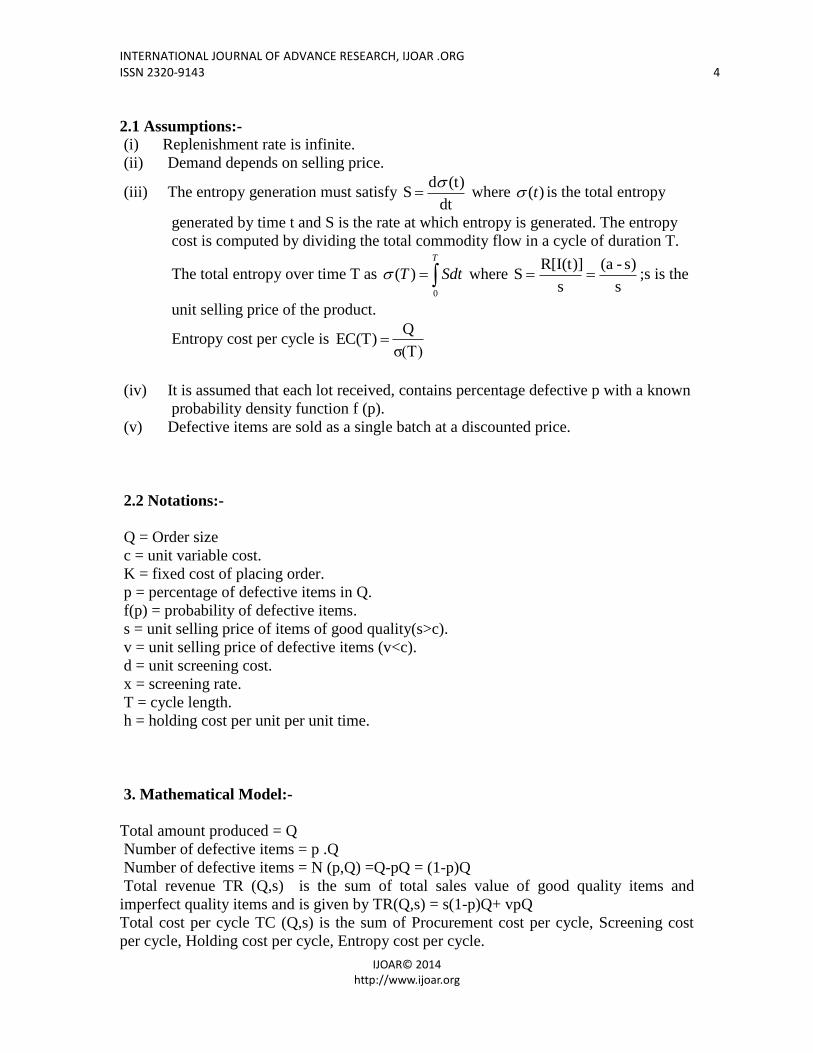
2.1 Assumptions:-

(i) Replenishment rate is infinite.

(ii) Demand depends on selling price.

(iii) The entropy generation must satisfy dt

(t)dS

where )(t is the total entropy

generated by time t and S is the rate at which entropy is generated. The entropy

cost is computed by dividing the total commodity flow in a cycle of duration T.

The total entropy over time T as T

SdtT0

)( where s

s)-(a

s

R[I(t)]S ;s is the

unit selling price of the product.

Entropy cost per cycle is σ(T)

Q EC(T)

(iv) It is assumed that each lot received, contains percentage defective p with a known

probability density function f (p).

(v) Defective items are sold as a single batch at a discounted price.

2.2 Notations:-

Q = Order size

c = unit variable cost.

K = fixed cost of placing order.

p = percentage of defective items in Q.

f(p) = probability of defective items.

s = unit selling price of items of good quality(s>c).

v = unit selling price of defective items (v<c).

d = unit screening cost.

x = screening rate.

T = cycle length.

h = holding cost per unit per unit time.

3. Mathematical Model:-

Total amount produced = Q

Number of defective items = p .Q

Number of defective items = N (p,Q) =Q-pQ = (1-p)Q

Total revenue TR (Q,s) is the sum of total sales value of good quality items and

imperfect quality items and is given by TR(Q,s) = s(1-p)Q+ vpQ

Total cost per cycle TC (Q,s) is the sum of Procurement cost per cycle, Screening cost

per cycle, Holding cost per cycle, Entropy cost per cycle.



Thus,TC(Q,s) =OC+ PC+SRC+HC+EC

The differential equation governing instantaneous state of q (t) at some instant of time t is

given by

s)(adt

dq(t) (1)

with the initial boundary condition q (0) = (1-p) Q (1a)

q (T) = 0 (1b)

Solving (1) and using the boundary condition (1a), we get

q (t) = ((1-p) Q – (a-s)t (2)

Now, q (T) = 0 gives

s)(a

p)Q(1T

(3)

(1) Cost of Placing Order per cycle(OC) = K (4)

(2) Cost of Purchasing Units per cycle(PC) = c Q (5)

(3) Screening Cost per cycle(SRC) =d Q (6)

(4) Cost of Carrying Inventory in the cycle

hpQτs)t]dt(ap)Q[(1hhpQτq(t)dthHC

T

τ

T

τ

=x

hpQ

2

)τ(Ts)(aτ)-p)Q(T(1h

222

=

x

pQ

x

Q

s)(a

Qp)(1

2

s)(a

x

Q

s)(a

p)Q(1p)Q(1h

2

2

2

2

22

(7)

Again s

D(T) (T) where s)T(as)dt(aR(s)dtD(T)

T

0

T

0

(5)Cost of Entropy in the cycle is σ(T)

QEC =

D(T)

Qs =

s)T-(a

Qs =

p)-(1

s (8)

Using the equation (4) to (8), Total Inventory Cost (TC) is

TC (Q,s) = OC+PC + SRC+ HC + EC

= K + cQ + dQ + HC + EC

TC (Q, s) = K + cQ + dQ +

x

pQ

x

Q

s)(a

Qp)(1

2

s)(a

x

Q

s)(a

p)Q(1p)Q(1h

2

2

2

2

22

+p)-(1

s (9)



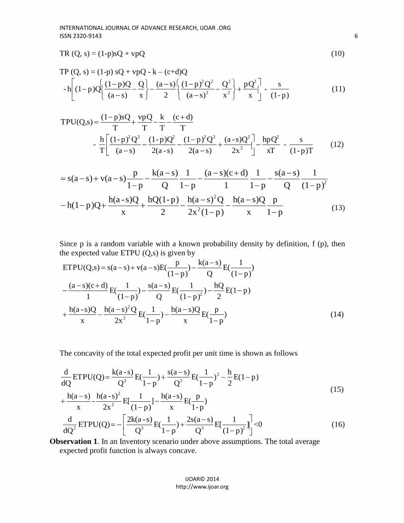
TR (Q, s) = (1-p)sQ + vpQ (10)

TP (Q, s) = (1-p) sQ + vpQ - k – (c+d)Q

-

x

pQ

x

Q

s)(a

Qp)(1

2

s)(a

x

Q

s)(a

p)Q(1p)Q(1h

2

2

2

2

22

-p)-(1

s (11)

T

d)(c

T

k

T

vpQ

T

p)sQ(1s)TPU(Q,

- xT

hpQ

2x

s)Q-(a

s)2(a

Qp)(1

s)-2(a

p)Q-(1

s)(a

Qp)-(1

T

h 2

2

222222

-

p)T-(1

s (12)

p1

p

x

s)Qh(a

p)(12x

Qs)h(a

2

p)-hQ(1

x

s)Q-h(ap)Qh(1

p)(1

1

Q

s)s(a

p1

1

1

d)s)(c(a

p1

1

Q

s)k(a

p1

ps)v(as)s(a

2

2

2

(13)

Since p is a random variable with a known probability density by definition, f (p), then

the expected value ETPU (Q,s) is given by

)p1

pE(

x

s)Qh(a)

p1

1E(

2x

Qs)h(a

x

s)Q-h(a

p)E(12

hQ)

p)(1

1E(

Q

s)s(a)

p)(1

1E(

1

d)s)(c(a

)p)(1

1E(

Q

s)k(a)

p)(1

ps)E(v(as)s(as)ETPU(Q,

2

2

2

(14)

The concavity of the total expected profit per unit time is shown as follows

)p-1

pE(

x

s)-h(a]

p)(1

1E[

2x

s)-h(a-

x

s)h(a

p)E(12

h)

p1

1E(

Q

s)s(a)

p1

1E(

Q

s)-k(a ETPU(Q)

dQ

d

2

2

2

22

(15)

]

p)(1

1E[

Q

s)2s(a)

p1

1E(

Q

s)-2k(a ETPU(Q)

dQ

d2332

<0 (16)

Observation 1. In an Inventory scenario under above assumptions. The total average

expected profit function is always concave.



)p1

1E(

x

hQ)

p)(1

1E(

2x

s)-2h(a

Q

hQ-)

p1

1E(

Q

2s p)E(1

Q

a

)p1

1d)E((c)

p1

1E(

Q

k)

p1

pvE(-2s-a s)ETPU(Q,

ds

d

22

(17)

})

p1

1{E(

Q

2-)

p)(1

1E(2 s)ETPU(Q,

ds

d 2

22 x

hQ < 0 (18)

provided ]p)(1

1E[)

p1

1E(Q

2

This leads to the following observation

Observation 2. In an Inventory scenario under above assumptions, the total expected average

profit function is always concave w.r.t. selling price p.

Since p is uniformly distributed

otherwise ; 0

0.04 p 0 ; 25

f(p)

dpp1

p)(1125dp

p1

25p)

p1

pE(

0.04

0

0.04

0

= 0.02055

dpp1

25)

p1

1E(

0.04

0

= 1.02055

16.66 dpp)(1

25]

p)(1

1E[

0.04

0

22

08.0p)dp(125p)E(1

0.04

0

4.1 Numerical Results:-

Here, k = 100/cycle

h = 5 unit

x = 1 unit/min

d = $ 0.5/unit

c = $ 25/unit

v = $ 20/unit

x = 1*60*8*365 = 175200

(Assuming that the inventory system operates on an 8 hours/day for 365 days a year. Then

annual screening rate x = 1*60*8*365 = 175200 units/year

Q, s = decision variable



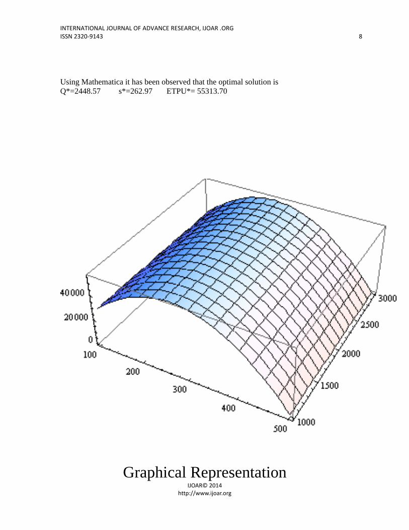
Using Mathematica it has been observed that the optimal solution is

Q*=2448.57 s*=262.97 ETPU*= 55313.70

Graphical Representation



Table-2 (Sensitivity Analysis)

Parameter Value EOQ(Q*) Selling Price(s*) Expected Profit

(ETPU)

h

2

3

5

8

10

3871.34

3060.65

2448.57

1935.73

1731.35

262.87

262.88

262.97

263.01

263.03

55661.80

55550.50

55313.70

55062.90

54921.50

a

100

200

500

800

1000

481.21

958.36

2448.57

3968.02

4999.61

63.48

113.36

262.97

412.91

512.88

1191.40

7223.91

55313.70

148417.00

235494.01

c

10

20

25

30

40

2456.55

2451.46

2448.57

2445.44

2438.48

255.26

260.39

262.97

265.53

270.67

59001.30

56529.80

55313.70

54110.70

51744.10

d

0.2

0.3

0.5

0.7

0.8

2448.75

2448.69

2448.57

2448.45

2448.39

262.81

262.86

262.97

263.07

263.12

55386.30

553662.10

55313.70

55265.40

55241.20



§ 4.2 Result Discussion:

From the sensitivity analysis(Table-2),the following results can be deducted

(i) As the holding cost (h) increases, the economic order quantity (EOQ) decreases and

obviously the expected total average profit also decreases which is quite relevant in real

life situation.As holding cost increases,selling price has also been increased.

(ii) EOQ & ETPU increases significantly when the parameter “a” increases, i.e. the parameter

a is highly sensitive w.r.t EOQ & ETPU.

(iii)As the purchase cost (c) increases EOQ andETPU decreases in a moderate way which is

also true in practice.

(iv)The change in the parameter “d” affects on EOQ & ETPU very little.

5. Conclusion:

In this paper an entropic order quantity model is developed where demand depends on selling

price. A screening is also done to differentiate good quality items and defectives items.

Numerical analysis reveals that expected total average profit has proportional relations with

the carrying cost and purchase cost which is very realistic in practice.

Several possible extensions of the present model could enlighten the future research

endeavors in this field.No doubt selling price plays an important role to influence the demand

of a commodity but it is no denying fact that price as well as on hand stock inventory are also

important on influencing the demand of a product. Thus demand may be considered

multivariate function of time, price and on hand stock level. The model proposed here may

also be extended by introducing shortage, partial backlogging, inflation, credit period

deterioration and so on.



6. References:-

[1] Abad,P.L.(1996), „Optimal pricing and lot-sizing under conditions of perishibility and partial

backordering‟,Management Science,vol. 42,no. 8,pp. 1093-1104.

[2] Abad,P.L.(2007), „Optimal pricing and lot-sizing under partial backordering incorporating

shortage,backorder and lost sale costs‟,International Journal of Production

Economics,vol.114,no.1,pp. 179-186.

[3] Bernstein,F and Federgruen,A.(2004), „Dynamic inventory and pricing models for

competing retailers.‟Naval Research Logistics,vol.51,pp. 248-274.

[4] Burewell,T.H.;Dave,D.S.,Fitzpatrick,K.E. and Roy,M.R.(1991), „An inventory model with

planned shortages and price dependent demand‟.Decisions Science,vol.27,pp. 1181-1191.

[5] Cardenes-Barron Le (2009), „Observation on economic production quantity model for items

with imperfect quantity‟, International Journal of Production Economics, 67, 59-64.

[6] Chang,H.J. ;Teng,J.T.;Ouyang,L.Y and Dye,C.Y.(2006), „Retailer‟s optimal pricing and lot-

sizing policies for deteriorating items with partial backlogging‟,European Journal of

Operational Research‟vol.168.no. 1,pp. 51-64.

[7] Chung,H.C.(2004), „ An application of fuzzy sets theory to the EOQ model with imperfect

quality items‟, Computer & Operations Research,31,2079-2092.

[8] Chung,Y.D.;Tsu,P.H. & Liang,Y(2007), „Determining optimal selling price and lot-size

with a varying rate of deterioration and exponential partial backlogging.‟European Journal

of Operational Research,181,668-678.

[9] Eroglu,A and Ozdemir,A.(2007), „An economic order quantity model with defective items

and shortages‟,International Journal of Production Economics,106,pp. 544-549.

[10]Jabber,M.Y.(2007), „Lot-sizing with permissible delay in payments and entropy

cost‟,Computers and Industrial Engineering,vol.52(1),pp. 78-88.

[11] Jaber,M.Y. ;Bonny,M ;Rosen,M.A. & Moualek,I.(2008), „Entropic Order quantity(EnOQ)

Model for deteriorating items‟. Applied Mathematical Modeling.

[12] Jaber,M.Y. ;Goyal,S.K. & Imran,M (2008) , „Economic production quantity model for

items with imperfect quality subject to learning effects‟, International Journal of

ProductionEconomics,115,143-150.

[13] Kar,S.;Roy,T. and Maity,M. (2001), „Multi-item inventory model with probabilistic price

dependent demand and imprecise goal and constraints‟,Yogoslav Journal of Operational

Research,vol. 11,no. 1,pp 93-103.

[14] Kim,J.;Hwang,H and Shinn,S.W.(1995), „An optimal credit policy to increase supplier‟s

profit with price-dependent demand functions‟,Production,Planning and Control,vol.

6(1),pp.45-50.

[15] Lin,T.Y.(2010), „Optimal policy for a simple supply chain system with defective items and

returned cost under screening errors‟, Journal of Operational Research Society,52,307-320.

[16] Maddah, B & Jaber, M.Y. (2008) „Economic order quantity for items with imperfect

quantity‟, International Journal of Production Economics, 112,808-815.

[17] Papachristo, S & Konstantaras,I.(2006), „Economic order quantity models for items with

imperfect quantity‟, International Journal of Production Economics,100,148-154.

[18] Pattnaik, M. (2010), „An entropic order quantity (EOQ) model under instant deterioration

of perishable items with price discounts‟, International Mathematical Forum, 5(52),

2581-2590.

[19] Pattnaik, M. (2011), „An entropic order quantity (EnOQ) model with post cash discounts‟,

International Journal of Contemp Math, 6(19), 931-939.



[20] Porteus, E.L. (1986), „Optimal lot-sizing process quantity improvement and set-up cost

reduction‟, Operations Research,34,137-144.

[21] Rosenblatt, M.J. & Lee, H.L. (1986), „Economic production cycles with imperfect

production process‟, IIE Trans, 18,48-55.

[22] Roy,M.D.; Sana,S.S. and Chaudhuri,K.(2011), „An economic order quantity model of

imperfect quality items with partial backlogging‟,Internatioanl Journal of System

Science,vol.42,no. 8,pp. 1409-1419.

[23] Sabahno,H(2009), „Optimal policy for a deteriorating inventory model with finite

replenishment rate and with price dependent demand rate and cycle length dependent

price‟,International Journal of Human and Social Sciences,vol 4,no.15,pp. 1108-1112.

[24] Salameh, M.K. & Jaber, M.K. (2000), „Economic production quantity model for the items

with imperfect quantity‟, International Journal of Production Economics.64,(13),59-64.

[25] Sana,S.S.(2010), „Optimal selling price and lot size with time varying deterioration and

partial backlogging‟,Applied mathematics and Computation,vol217,no1,pp. 185-194.

[26] Teng,J.T and Chang,C.T.(2005), „Economic production quantity models for deteriorating

items with price and stock dependent demand‟,Computers and Operations

Research,vol.32,pp. 297-308.

[27] Tripathy,P.K and Pattnik,M.(2008), „An entropic order quantity model with fuzzy holding

cost and fuzzy disposal cost for perishable items under two component demand and

discounted selling price‟,Pak.Journal Stat.Oper.Research,vol.4,no. 2,pp 93-110.

[28] Yang,P.C.(2004), „Pricing strategy for deteriorating items using quantity discount when

demand is price sensitive.‟,European Journal of Operational Research,vol.157,pp. 389-

397

[29] Yoo, S.H.: Kim, D & Park, M.S. (2009), „Economic production quantity model with

imperfect quantity items, two-way imperfect inspection and sales return‟, International

Journal of Production Economics.

[30] Wee, H.M. & Chen, M.C. (2007), „Optimal inventory model for items with imperfect

quantity and shortage backordering‟, Omega, 35, 7-11.

[31] Zhang,X and Gerchak,Y.(1991), „Joint lot-sizing and inspection policy in an EOQ model

with random yield‟,IIE Trnasaction,vol.22,no.1,pp 41.

international journal of advance research, ijoar fileeoq model is that all units purchased or...

Documents