international financial markets 1. how capital markets work prof. dr. rainer maurer -1- lecture...
Post on 20-Dec-2015
220 views
TRANSCRIPT
International Financial Markets1. How Capital Markets Work
Prof. Dr. Rainer Maurer -1-
Lecture Notes: www.rainer-maurer.deE-Mail: [email protected]: Friday 17.15 - 18.45 (room W1.4.03)
1. How Capital Markets Work
1. How Capital Markets Work1.1. Supply and Demand on Capital Markets
1.1.1. Why People Save1.1.2. Why People Invest1.1.3. Investor and Saver Surplus
1.2. Capital Markets and Risk1.2.1. Why People Don’t Like Risk1.2.2. How People Handle Risk
1.3. Basic Evaluation Techniques for Capital Markets1.3.1. The Discounted Cash-Flow Method1.3.2. The Internal Rate of Return Method 1.3.3. Risk and Return: The Sharpe Ratio
2. Questions for Review
Literature:1)
◆ Chapter 4, 25, Mankiw, N.G. (2001): Principles of Economics, Harcourt Coll. Publ., Orlando.◆ Chapter 7, Mankiw, N.G. (2002): Macroeconomics, Worth Publishers, New York.
Prof. Dr. Rainer Maurer -2-1) The recommended literature typically includes more content than necessary for an understanding of this chapter. Relevant for the examination is the content of this chapter as presented in the lectures.

1. How Capital Markets Work1.1.1. Why People Save
1. How Capital Markets Work1.1. Supply and Demand on Capital Markets
1.1.1. Why People Save1.1.2. Why People Invest
1.2. Capital Markets and Risk 1.2.1. Why People Don’t Like Risk
1.2.2. How People Handle Risk1.3. Basic Evaluation Techniques for Capital Markets
1.3.1. The Discounted Cash-Flow Method1.3.2. The Internal Rate of Return Method1.3.3. Risk and Return: The Sharpe Ratio
Prof. Dr. Rainer Maurer -3-

1. How Capital Markets Work1.1.1. Why People Save
Prof. Dr. Rainer Maurer -4-
1. How Capital Markets Work1.1.1. Why People Save
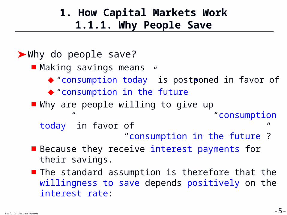
➤ Why do people save?■Making savings means
◆“consumption today” is postponed in favor of
◆“consumption in the future”
■Why are people willing to give up “consumption today” in favor of “consumption in the future”?
■Because they receive interest payments for their savings.
■The standard assumption is therefore that the willingness to save depends positively on the interest rate:
Prof. Dr. Rainer Maurer -5-

The Slope of the Savings Curve
Prof. Dr. Rainer Maurer -6-
0%
2%
4%
6%
8%
10%
0 1 2 3 4 5 6 7 8 9 10 11 12 13 14 15 16 17 18 19 20
Savings = S(i)
%
€
Why do people save more, when
they receive higher interest payments?
Higher interest payments allow for “higher consumption in the future”. This compensates for
the “lower consumption today”.

1. How Capital Markets Work1.1.1. Why People Save
➤ How does this affect consumption of households?
➤ The relationship between “savings today” and “consumption today” is inverse.
➤ The budget constraint of a household shows this. If we neglect the necessity to pay taxes, the simplest form a budget constraint is given by the equation:
Income = Savings + Consumption
Y = S + C
<=> C = Y – S
<=> C(i ) = Y – S(i )
Prof. Dr. Rainer Maurer -7-
+-
[ ]
The Slope of the Savings Curve
Prof. Dr. Rainer Maurer -8-
0%
2%
4%
6%
8%
10%
0 1 2 3 4 5 6 7 8 9 10 11 12 13 14 15 16 17 18 19 20
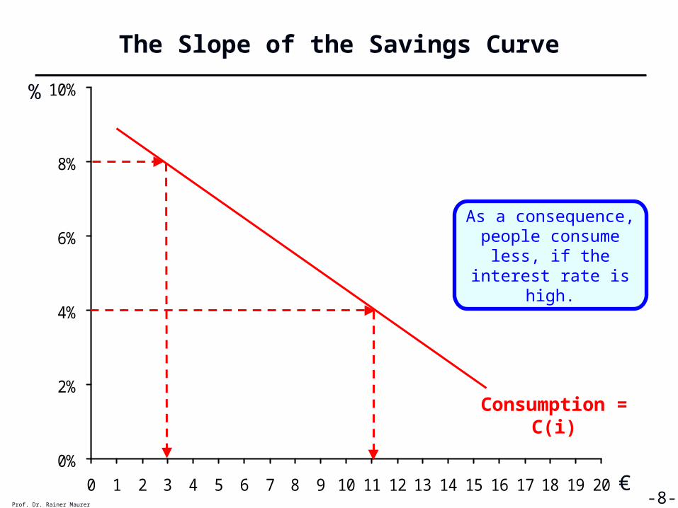
Consumption = C(i)
As a consequence, people consume
less, if the interest rate is high.
%
€

1. How Capital Markets Work1.1.1. Why People Save
➤ How does an increase of permanent income affect the savings function?
Y = S + C
➤ It must increase savings and/or consumption.
➤ Most likely is that it increases both savings and consumption at the same time, because a permanent increase of income means that higher income will also be available in future periods. So people have no reason to postpone current consumption into the future.
Prof. Dr. Rainer Maurer -9-

The Slope of the Savings Curve
Prof. Dr. Rainer Maurer -10-
0%
2%
4%
6%
8%
10%
0 1 2 3 4 5 6 7 8 9 10 11 12 13 14 15 16 17 18 19 20
Savings = S(i, y1)
Savings = S(i, y2)
%
€
How does an increase of permanent income
“y” change the willingness to save?
If the permanent income of households y2 > y1
grows, households will typically save more!

The Slope of the Savings Curve
Prof. Dr. Rainer Maurer -11-
0%
2%
4%
6%
8%
10%
0 1 2 3 4 5 6 7 8 9 10 11 12 13 14 15 16 17 18 19 20
Savings = S(i, y1)
Therefore household permanent income “y” is a shift parameter of the
savings function!
Savings = S(i, y2)
%
€

The Slope of the Savings Curve
Prof. Dr. Rainer Maurer -12-
0%
2%
4%
6%
8%
10%
0 1 2 3 4 5 6 7 8 9 10 11 12 13 14 15 16 17 18 19 20
Savings = S(i, y1)
If the permanent income of households y2 < y1
decreases, households will typically save less!
Savings = S(i, y2)%
€
1. How Capital Markets Work1.1.1. Why People Save
1. How Capital Markets Work1.1. Supply and Demand on Capital Markets
1.1.1. Why People Save1.1.2. Why People Invest
1.2. Capital Markets and Risk 1.2.1. Why People Don’t Like Risk
1.2.2. How People Handle Risk1.3. Basic Evaluation Techniques for Capital Markets
1.3.1. The Discounted Cash-Flow Method1.3.2. The Internal Rate of Return Method1.3.3. Risk and Return: The Sharpe Ratio
Prof. Dr. Rainer Maurer -14-
1. How Capital Markets Work1.1.2. Why People Invest
➤ Why do people invest?■Investment means
◆ to spend money for “economic activities today”, which are assumed to yield a “return in the future”
■Investment projects can be ranked according to their expected return.
■This yields the following curve:
Prof. Dr. Rainer Maurer -15-

The Slope of the Investment Curve
Prof. Dr. Rainer Maurer -16-
0%
1%
2%
3%
4%
5%
6%
7%
8%
9%
10%
0 1 2 3 4 5 6 7 8 9 10 11 12 13 14 15 16 17 18 19 20
%
€
Expected return
Available investment projects depending on their expected return
and investment volume
Investment volume of the first project

The Slope of the Investment Curve
Prof. Dr. Rainer Maurer -17-
0%
1%
2%
3%
4%
5%
6%
7%
8%
9%
10%
0 1 2 3 4 5 6 7 8 9 10 11 12 13 14 15 16 17 18 19 20
If the market interest rate is 8%, only the first
investment project is profitable! All other
investment projects are not undertaken!
Interest rate: 8%
%
€

0%
1%
2%
3%
4%
5%
6%
7%
8%
9%
10%
0 1 2 3 4 5 6 7 8 9 10 11 12 13 14 15 16 17 18 19 20
The Slope of the Investment Curve
Prof. Dr. Rainer Maurer -18-
If the market interest rate is 2%, only the first five investment projects are
profitable!
Interest rate: 2%
%
€

The Slope of the Investment Curve
Prof. Dr. Rainer Maurer -19-
0%
1%
2%
3%
4%
5%
6%
7%
8%
9%
10%
0 1 2 3 4 5 6 7 8 9 10 11 12 13 14 15 16 17 18 19 20
If we add the savings curve to the curve of available investment projects we recognize, how many
investment projects savers are willing to finance: %
€
Savings = S(i)
The Slope of the Investment Curve
Prof. Dr. Rainer Maurer -20-
0%
1%
2%
3%
4%
5%
6%
7%
8%
9%
10%
0 1 2 3 4 5 6 7 8 9 10 11 12 13 14 15 16 17 18 19 20
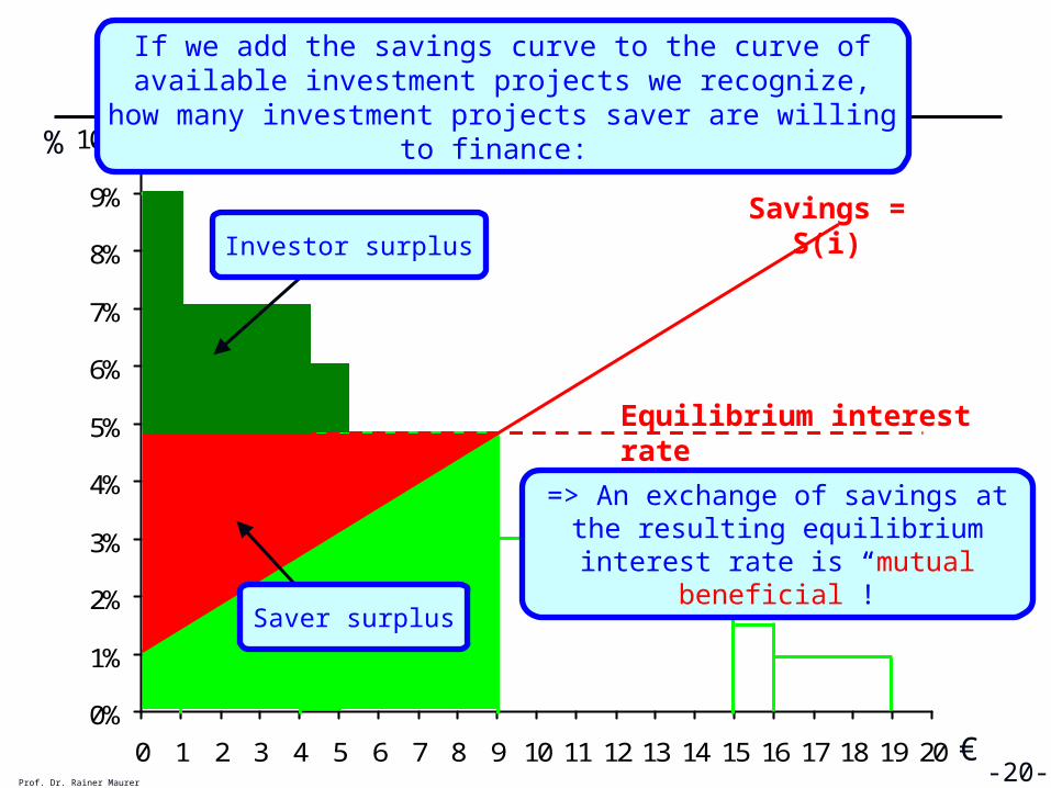
If we add the savings curve to the curve of available investment projects we recognize, how many
investment projects saver are willing to finance: %
€
Savings = S(i)
Equilibrium interest rate
Saver surplus
=> An exchange of savings at the resulting equilibrium interest
rate is “mutual beneficial”!
Investor surplus

The Slope of the Investment Curve
Prof. Dr. Rainer Maurer -21-
0%
1%
2%
3%
4%
5%
6%
7%
8%
9%
10%
0 1 2 3 4 5 6 7 8 9 10 11 12 13 14 15 16 17 18 19 20
In the following, we will for simplicity approximate the curve of investment projects with a straight line:
%
€
Savings = S(i)
Investment = I(i)

The Slope of the Investment Curve
Prof. Dr. Rainer Maurer -22-
0%
1%
2%
3%
4%
5%
6%
7%
8%
9%
10%
0 1 2 3 4 5 6 7 8 9 10 11 12 13 14 15 16 17 18 19 20
In the following, we will for simplicity approximate the curve of investment projects with a straight line:
%
€
Savings = S(i)
Investment = I(i)
Market interest rate
Saver surplus
Investor surplus

The Slope of the Investment Curve
Prof. Dr. Rainer Maurer -23-
0%
2%
4%
6%
8%
10%
0 1 2 3 4 5 6 7 8 9 10 11 12 13 14 15 16 17 18 19 20
Investment = I(i)
Contrary to the savings curve, the investment curve depends on the
negatively interest rate!
%
€
The investment curve is also influenced by shift
parameters, e.g. the expected return of
investment projects, r1!

The Slope of the Investment Curve
Prof. Dr. Rainer Maurer -24-
0%
2%
4%
6%
8%
10%
0 1 2 3 4 5 6 7 8 9 10 11 12 13 14 15 16 17 18 19 20
Investment = I(i,r1)
If firms expect on average a higher return on investment r1<r2
(e.g. because of an expected higher demand for their goods),
the investment curve shifts to the right!
Investment = I(i,r2)
%
€

The Slope of the Investment Curve
Prof. Dr. Rainer Maurer -25-
0%
2%
4%
6%
8%
10%
0 1 2 3 4 5 6 7 8 9 10 11 12 13 14 15 16 17 18 19 20
Investment = I(i,r1)
If firms expect a lower return on investment r1>r2 (e.g. because of a lower demand for their goods), they will typically want to
invest less.
Investment = I(i,r2)
%
€

The Capital Market
Prof. Dr. Rainer Maurer -26-
0%
1%
2%
3%
4%
5%
6%
7%
8%
9%
10%
0 1 2 3 4 5 6 7 8 9 10 11 12 13 14 15 16 17 18 19 20
I(i)
S(i,y)
i1*
S1*
Combination of the savings
supply curve and investment
demand curveEquilibrium Interest Rate
%
€

Prof. Dr. Rainer Maurer -27-
0%
1%
2%
3%
4%
5%
6%
7%
8%
9%
10%
0 1 2 3 4 5 6 7 8 9 10 11 12 13 14 15 16 17 18 19 20
I(i)
S1(i,y1)
i1*
S1*
S2(i,y2)
i2*
S2*
The Capital Market
%
€
y1 < y2

Prof. Dr. Rainer Maurer -28-
0%
1%
2%
3%
4%
5%
6%
7%
8%
9%
10%
0 1 2 3 4 5 6 7 8 9 10 11 12 13 14 15 16 17 18 19 20
I1(i , r1)
S(i)
I2(i, r2)
i1*
S1*
i2*
S2*
The Capital Market
%
€
r1 < r2
1. How Capital Markets Work 1.2.1. Why People Don’t Like Risk
1. How Capital Markets Work1.1. Supply and Demand on Capital Markets
1.1.1. Why People Save1.1.2. Why People Invest
1.2. Capital Markets and Risk 1.2.1. Why People Don’t Like Risk
1.2.2. How People Handle Risk1.3. Basic Evaluation Techniques for Capital Markets
1.3.1. The Discounted Cash-Flow Method1.3.2. The Internal Rate of Return Method1.3.3. Risk and Return: The Sharpe Ratio
Prof. Dr. Rainer Maurer -29-
1. How Capital Markets Work 1.2.1. Why People Don’t Like Risk
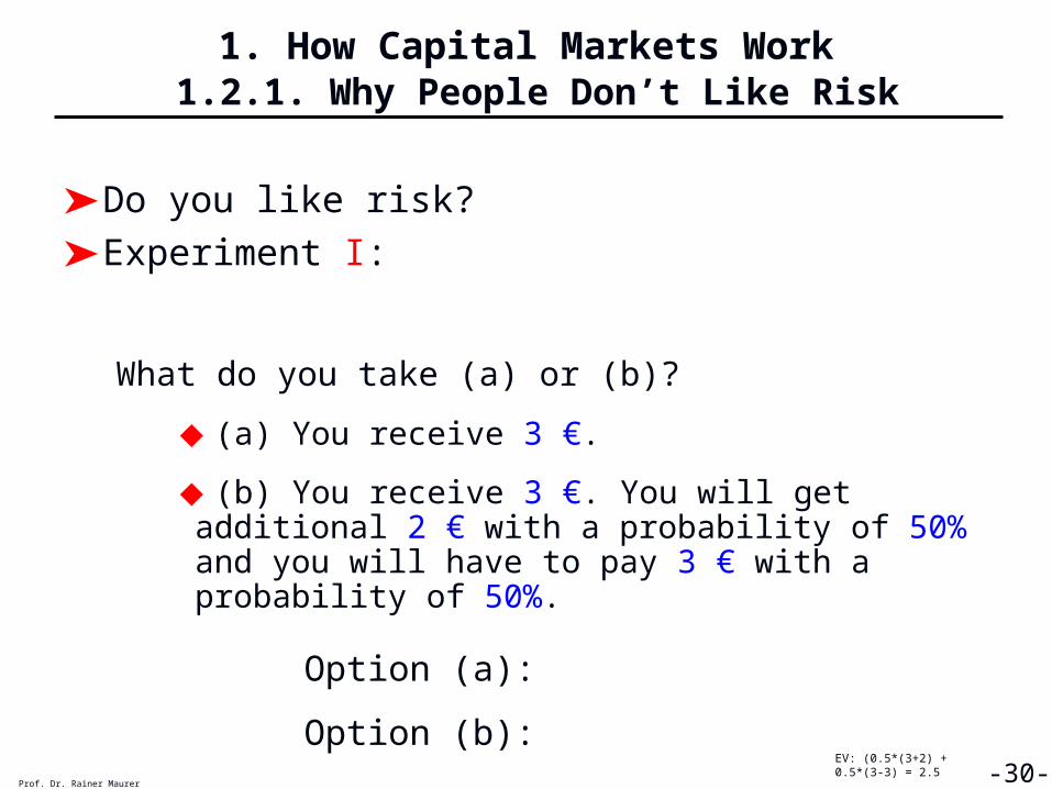
➤ Do you like risk?
➤ Experiment I:
What do you take (a) or (b)?
◆(a) You receive 3 €.
◆(b) You receive 3 €. You will get additional 2 € with a probability of 50% and you will have to pay 3 € with a probability of 50%.
Prof. Dr. Rainer Maurer -30-
Option (a):
Option (b): EV: (0.5*(3+2) + 0.5*(3-3) = 2.5

1. How Capital Markets Work 1.2.1. Why People Don’t Like Risk
➤ Do you like risk?
➤ Experiment II:
What do you take (a) or (b)?
◆(a) You receive 3 €.
◆(b) You receive 3 €. You will get additional 2 € with a probability of 50% and you will have to pay 2 € with a probability of 50%.
Prof. Dr. Rainer Maurer -31-
Option (a):
Option (b): EV: (0.5*(3+2) + 0.5*(3-2) = 3

1. How Capital Markets Work 1.2.1. Why People Don’t Like Risk
➤ Do you like risk?
➤ Experiment III:
What do you take (a) or (b)?
◆(a) You receive 3 €.
◆(b) You receive 3 €. You will get additional 7 € with a probability of 50% and you will have to pay 1 € with a probability of 50%.
Prof. Dr. Rainer Maurer -32-
Option (a):
Option (b): EV: (0.5*(3+7) + 0.5*(3-1) = 6

1. How Capital Markets Work 1.2.1. Why People Don’t Like Risk
➤ What does the experiment show?■Most people prefer a certain payment over a risky payment.■A risky payment is accepted only if it includes a premium,
which is “high enough”. In economics this premium is called “risk premium”.
■The magnitude of this “risk premium” individually differs from person to person.
■However, the existence of a risk premium shows that people generally do not like risk: They are willing to accept risk only, if they are compensated for the risk by a higher payment!
■In economics we call this “being risk averse”.
Prof. Dr. Rainer Maurer -33-

2,0
3,0
4,0
5,0
6,0
7,0
8,0
1999
-01
1999
-07
2000
-01
2000
-07
2001
-01
2001
-07
2002
-01
2002
-07
2003
-01
2003
-07
2004
-01
2004
-07
2005
-01
2005
-07
2006
-01
2006
-07
2007
-01
2007
-07
2008
-01
2008
-07
2009
-01
2009
-07
2010
-01
Industrieobligationen Bundeswertpapiere
Average Yields of Fixed Rate Securities with Time to Maturity above 3 Years of Different German Issuers%
Prof. Dr. Rainer Maurer- 34 -
Sou
rce
: D
euts
che
Bu
ndes
bank
= Corporate Bonds = Government Bonds
Empirical example for a risk premium:

1. How Capital Markets Work 1.2.1. Why People Don’t Like Risk
➤ Why do people demand a risk premium?■Our "self-experiment" and empirical data from financial markets
clearly show that people are risk averse and demand risk premiums for risky investments.
■Now the question is, why do people behave this way?■Is it "irrational fear" to be "risk averse" or can we explain it?■The next slides show the standard microeconomic explanation
for risk averse behavior. ◆Standard microeconomics derives the explanation from a quite
plausible property of the utility function of people: Decreasing marginal utility of consumption.
◆The next slide gives an explanation of this property:
Prof. Dr. Rainer Maurer -37-

1. How Capital Markets Work 1.2.1. Why People Don’t Like Risk
Prof. Dr. Rainer Maurer -38-
0
1
2
3
4
5
6
7
8
9
10
11
12
13
14
0 1 2 3 4 5 6 7 8 9 10 11 12 13 14 15 16 17 18 19 20
Utility from the Consumption of Cookies per Day
Quantity of Cookies (kg)
Utility = U(Cookies)
Utility from the Con-
sumption of 16 Cookies = 12 “Utils”
Utility of the 1st Cookie
Utility of the 2nd Cookie
…and so on
1. How Capital Markets Work 1.2.1. Why People Don’t Like Risk
Prof. Dr. Rainer Maurer -39-
-2-10123456789
10111213141516
0 1 2 3 4 5 6 7 8 9
Utility Units
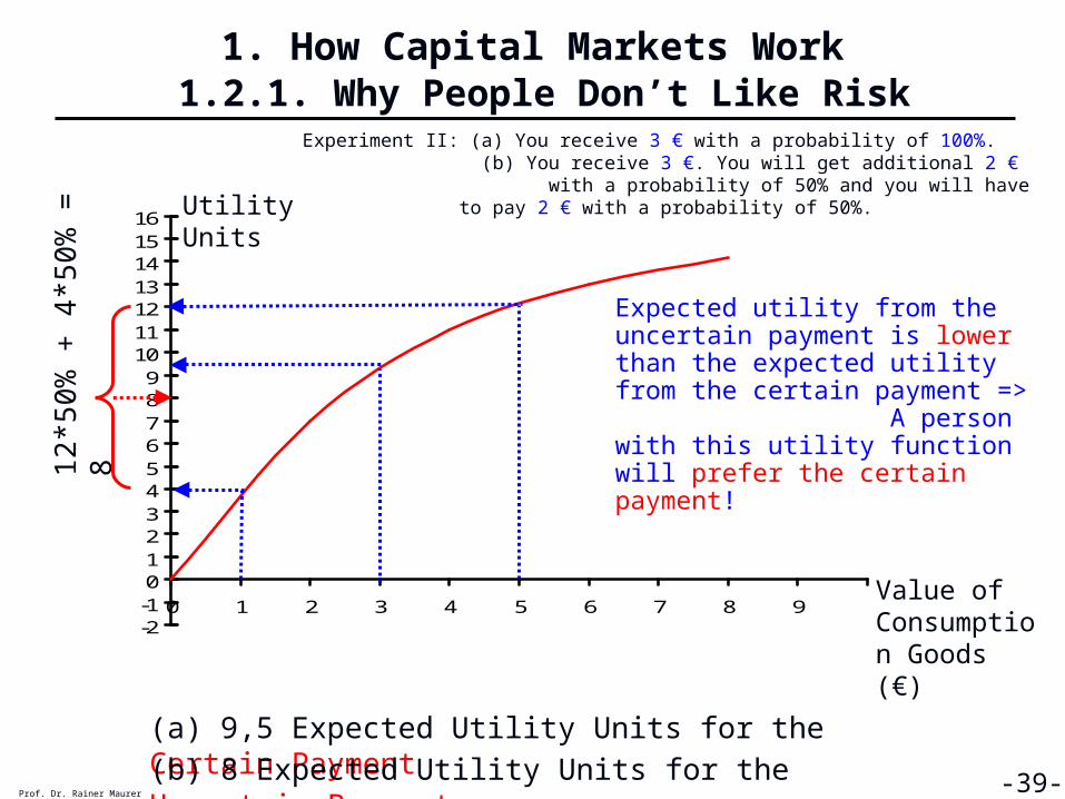
(a) 9,5 Expected Utility Units for the Certain Payment
Value of Consumption Goods (€)
12*
50%
+ 4
*50
% =
8
(b) 8 Expected Utility Units for the Uncertain Payment
Expected utility from the uncertain payment is lower than the expected utility from the certain payment => A person with this utility function will prefer the certain payment!
Experiment II: (a) You receive 3 € with a probability of 100%. (b) You receive 3 €. You will get additional 2 € with a probability of 50% and you will have to pay 2 € with a probability of 50%.

1. How Capital Markets Work 1.2.1. Why People Don’t Like Risk
Prof. Dr. Rainer Maurer -40-
-2-10123456789
10111213141516
0 1 2 3 4 5 6 7 8 9
Utility Units
(a) 9,5 Expected Utility Units for the Certain Payment
Value of Consumption Goods (€)
(b) 8 Expected Utility Units for the Uncertain Payment
The reason for the lower expected utility is the stronger change of utility in case of a loss compared to the case of a gain, because of decreasing marginal utility!
Experiment II: (a) You receive 3 € with a probability of 100%. (b) You receive 3 €. You will get additional 2 € with a probability of 50% and you will have to pay 2 € with a probability of 50%.
Income Loss of 2 €
Utility Loss: 5,5
Income Gain of 2 €
Utility Gain:
2

1. How Capital Markets Work 1.2.1. Why People Don’t Like Risk
Prof. Dr. Rainer Maurer -41-
-2-10123456789
10111213141516
0 1 2 3 4 5 6 7 8 9
Utility Units
(a) 6 Expected Utility Units for the Certain Payment
Value of Consumption Goods (€)
(b) 6 Expected Utility Units for the Uncertain Payment
In case of a utility function with constant marginal utility, the utility gain in case of an income gain would be equal to the utility loss in case of an income loss and hence expected utility in case of a certain payment would be equal to expected utility of an uncertain payment!
Experiment II: (a) You receive 3 € with a probability of 100%. (b) You receive 3 €. You will get additional 2 € with a probability of 50% and you will have to pay 2 € with a probability of 50%.
Income Loss of 2 €
Utility Loss: 4
Income Gain of 2 €
Utility Gain: 4
1. How Capital Markets Work 1.2.1. Why People Don’t Like Risk
Prof. Dr. Rainer Maurer -43-
-2-10123456789
10111213141516
0 1 2 3 4 5 6 7 8 9 10
Utility Units
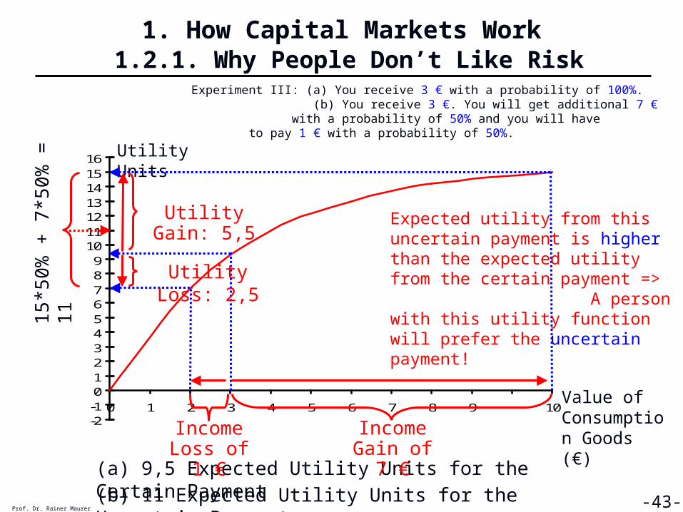
(a) 9,5 Expected Utility Units for the Certain Payment
Value of Consumption Goods (€)
15*
50%
+ 7
*50
% =
11
(b) 11 Expected Utility Units for the Uncertain Payment
Experiment III: (a) You receive 3 € with a probability of 100%. (b) You receive 3 €. You will get additional 7 € with a probability of 50% and you will have to pay 1 € with a probability of 50%.
Expected utility from this uncertain payment is higher than the expected utility from the certain payment => A person with this utility function will prefer the uncertain payment!
Income Loss of 1 €
Income Gain of 7 €
Utility Gain: 5,5
Utility Loss: 2,5

1. How Capital Markets Work 1.2.1. Why People Don’t Like Risk
Prof. Dr. Rainer Maurer -44-
-2-10123456789
10111213141516
0 1 2 3 4 5 6 7 8 9 10
Utility Units
Value of Consumption Goods (€)
Normal Person (Risk Averse) Utility Function
Gambler (Risk Lover) Utility Function
Risk Neutral Utility Function
Since we know from experiments that most people are risk averse, we can draw the conclusion that most people have a utility function with decreasing marginal utility!

1. How Capital Markets Work 1.2.2. How People Handle Risk
1. How Capital Markets Work
1.1. Supply and Demand on Capital Markets
1.1.1. Why People Save
1.1.2. Why People Invest
1.2. Capital Markets and Risk 1.2.1. Why People Don’t Like Risk
1.2.2. How People Handle Risk1.3. Basic Evaluation Techniques for Capital Markets
1.3.1. The Discounted Cash-Flow Method1.3.2. The Internal Rate of Return Method
1.3.3. Risk and Return: The Sharpe Ratio
Prof. Dr. Rainer Maurer -45-

1. How Capital Markets Work 1.2.2. How People Handle Risk
➤ We have already seen, how normal people handle risk:■They demand a risk premium!
➤ Financial markets offer a possibility to eliminate risk:■Hedging!
➤ The following tables illustrate the principle of hedging based on several numeric examples:
Prof. Dr. Rainer Maurer -46-

1. How Capital Markets Work 1.2.2. How People Handle Risk
➤ This example shows:■If the return of one stock goes up exactly when the return of the
other stock goes down, a portfolio of both stocks completely eliminates the risk!
■Consequently, investing your money in a portfolio of both stocks implies no risk, while investing your money in one of both stocks only implies a lot of risk!
■Note: In case of a perfect hedge, the correlation coefficient equals exactly -1!
Prof. Dr. Rainer Maurer -48-
Portfolio: (R. & S.) / 2 5,0 5,0 5,0 5,0 0
Stock Cloudy Sunny Rainy Mean VarianceRaincoat Corporation 13 -15 17 5,0 203Sunglasses International -3 25 -7 5,0 203
The Perfect Hedge
Corr. Coeff.
-1,0

1. How Capital Markets Work 1.2.2. How People Handle Risk
➤ This example shows:■If the return of one stock goes up exactly when the return of the
other stock goes up, a portfolio of both stocks does not affect risk at all!
■Consequently, investing your money in a portfolio of both stocks implies the same risk, as investing your money in one of both stocks only!
■Note: In case of a no hedge, the correlation coefficient equals exactly 1!
Prof. Dr. Rainer Maurer -49-
Portfolio: (R. & S.) / 2 15 -15 20 6,7 239
Stock Cloudy Sunny Rainy Mean VarianceRaincoat Corporation 15 -15 20 6,7 239Umbrella Unlimited 15 -15 20 6,7 239
No Hedge
Corr. Coeff.
1,0
Corr. Coeff.
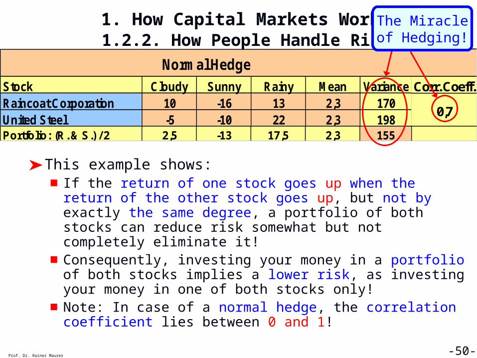
0,7
Portfolio: (R. & S.) / 2 2,5 -13 17,5 2,3 155
Stock Cloudy Sunny Rainy Mean VarianceRaincoat Corporation 10 -16 13 2,3 170United Steel -5 -10 22 2,3 198
Normal Hedge
1. How Capital Markets Work 1.2.2. How People Handle Risk
➤ This example shows:■If the return of one stock goes up when the return of the other
stock goes up, but not by exactly the same degree, a portfolio of both stocks can reduce risk somewhat but not completely eliminate it!
■Consequently, investing your money in a portfolio of both stocks implies a lower risk, as investing your money in one of both stocks only!
■Note: In case of a normal hedge, the correlation coefficient lies between 0 and 1!
Prof. Dr. Rainer Maurer -50-
The Miracle of Hedging!
1. How Capital Markets Work 1.2.2. How People Handle Risk
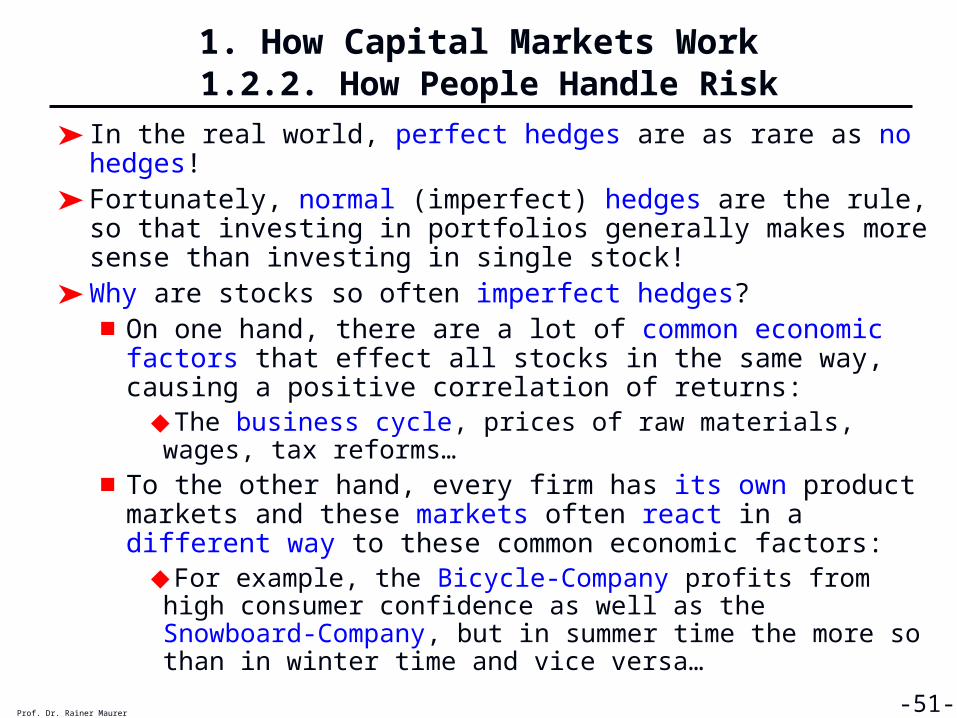
➤ In the real world, perfect hedges are as rare as no hedges!➤ Fortunately, normal (imperfect) hedges are the rule, so that
investing in portfolios generally makes more sense than investing in single stock!
➤ Why are stocks so often imperfect hedges?■On one hand, there are a lot of common economic factors that
effect all stocks in the same way, causing a positive correlation of returns:◆The business cycle, prices of raw materials, wages, tax
reforms…■To the other hand, every firm has its own product markets and
these markets often react in a different way to these common economic factors: ◆For example, the Bicycle-Company profits from high consumer
confidence as well as the Snowboard-Company, but in summer time the more so than in winter time and vice versa…
Prof. Dr. Rainer Maurer -51-

1. How Capital Markets Work 1.2.2. How People Handle Risk
➤ As the examples have shown, we can comfortably measure the hedge quality of two kind of stocks by the correlation coefficient.
➤ How do we compute the correlation coefficient?
Prof. Dr. Rainer Maurer -52-
5,0B)tockVariance(S*A)tockVariance(S
B)StockA,(StockCovariance

1. How Capital Markets Work 1.2.2. How People Handle Risk
➤ How do we compute the variance?
➤ How do we compute the covariance?
Prof. Dr. Rainer Maurer -53-
2A)ReturnsMean(All-jTimeatAReturnMean
A)Stock(ReturnVariance
B)ReturnsMean(All-jTimeatBReturn
*A)ReturnsMean(All-jTimeatAReturnMean
)B,StockReturnA,Stock(ReturnCovariance

1. How Capital Markets Work 1.2.2. How People Handle Risk
➤ Interpretation of the Correlation Coefficient:
Prof. Dr. Rainer Maurer -54-
➤ A correlation coefficient of -1 indicates that the value of two stocks moves through time with exactly opposite fluctuations:■If the stock of Raincoat Corp. displays a positive deviation from
its mean value, the stock of Sunglasses International displays a negative deviation form its mean value.
■If the stock of Raincoat Corp. displays a negative deviation from its mean value, the stock of Sunglasses International displays a positive deviation form its mean value.
Country 2002 2003 2004 2005 2006 2007 Correlation CoefficientRaincoat Corp. 1 -1 1 -1 1 -1Sunglasses International -1 1 -1 1 -1 1 -1

1. How Capital Markets Work 1.2.2. How People Handle Risk
➤ Interpretation of the Correlation Coefficient:
Prof. Dr. Rainer Maurer -55-
➤ A correlation coefficient of 1 indicates that the value of two stocks moves through time with exactly the same fluctuations:■If the stock of Raincoat Corp. displays a positive deviation from
its mean value, the stock of Umbrella Unlimited displays a positive deviation form its mean value too.
■If the stock of Raincoat Corp. displays a negative deviation from its mean value, the stock of Umbrella Unlimited displays a negative deviation form its mean value too.
Country 2002 2003 2004 2005 2006 2007 Correlation CoefficientRaincoat Corp. 1 -1 1 -1 1 -1Umbrella Unlimited 1 -1 1 -1 1 -1 1
1. How Capital Markets Work 1.2.2. How People Handle Risk
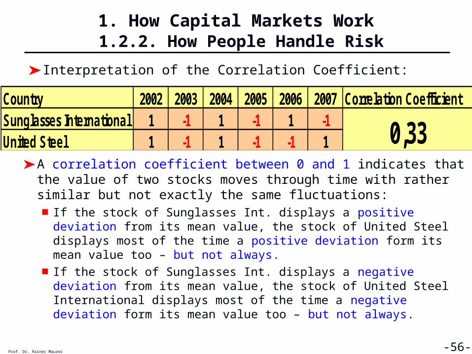
➤ Interpretation of the Correlation Coefficient:
Prof. Dr. Rainer Maurer -56-
➤ A correlation coefficient between 0 and 1 indicates that the value of two stocks moves through time with rather similar but not exactly the same fluctuations:■If the stock of Sunglasses Int. displays a positive deviation from its
mean value, the stock of United Steel displays most of the time a positive deviation form its mean value too – but not always.
■If the stock of Sunglasses Int. displays a negative deviation from its mean value, the stock of United Steel International displays most of the time a negative deviation form its mean value too – but not always.
Country 2002 2003 2004 2005 2006 2007 Correlation CoefficientSunglasses International 1 -1 1 -1 1 -1United Steel 1 -1 1 -1 -1 1 0,33

1. How Capital Markets Work 1.2.2. How People Handle Risk
➤ Now it’s up to you:■As portfolio manager you have to decide in the following cases,
whether to invest in single stock or in a portfolio.
■What do you recommend?
Prof. Dr. Rainer Maurer -57-

1. How Capital Markets Work 1.2.2. How People Handle Risk
Prof. Dr. Rainer Maurer -58-
Stock 2005 2006 2007 Variance Corr. Coeff.Pennylane Corp. 160 130 150MeanMean-DeviationSquared Mean-Deviation
Galapagos International 30 60 40MeanMean-DeviationSquared Mean-Deviation
Portfolio: (P. & G.) / 2MeanMean-DeviationSquared Mean-Deviation
Correlation Coefficient = Covariance / ( Variance * Variance)^0,5
Variance = Mean( Squared Mean Deviation )
Covariance = Mean( (Mean Deviation Stock A) * (Mean Deviation Stock B) )
Portfolio or not? What do you recommend?
1. How Capital Markets Work 1.2.2. How People Handle Risk
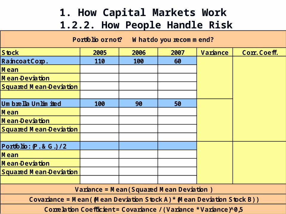
Prof. Dr. Rainer Maurer -59-
Stock 2005 2006 2007 Variance Corr. Coeff.Raincoat Corp. 110 100 60MeanMean-DeviationSquared Mean-Deviation
Umbrella Unlimited 100 90 50MeanMean-DeviationSquared Mean-Deviation
Portfolio: (P. & G.) / 2MeanMean-DeviationSquared Mean-Deviation
Correlation Coefficient = Covariance / ( Variance * Variance)^0,5
Variance = Mean( Squared Mean Deviation )
Covariance = Mean( (Mean Deviation Stock A) * (Mean Deviation Stock B) )
Portfolio or not? What do you recommend?

1. How Capital Markets Work 1.2.2. How People Handle Risk
➤ The Market-Beta:■As already seen, it is almost impossible to find perfectly negatively
correlated stocks – so that all portfolios end up with a risk that cannot be eliminated – the so called “market risk”.
■The market risk is measured by the variance of the average return of the market portfolio, i,e. the risk that cannot be eliminated by investing in the market portfolio.
■The tendency of the return of a stock to move with the average return of the market portfolio is called its market-beta.
■The market-beta is a measure of the relative volatility of a stock return compared to the return of the total stock market (= a portfolio consisting of all stocks minus the one stock whose beta is measured) as a whole.◆A beta of 1 means that a stock return moves exactly as the market does.◆A beta of 2 means that if a stock market return moves up by 10 %, the
stock return moves up by 20 %.
=> Adding a high (low) beta-stock to a portfolio means increasing (reducing) the portfolio risk.Prof. Dr. Rainer Maurer -60-
1. How Capital Markets Work 1.2.2. How People Handle Risk
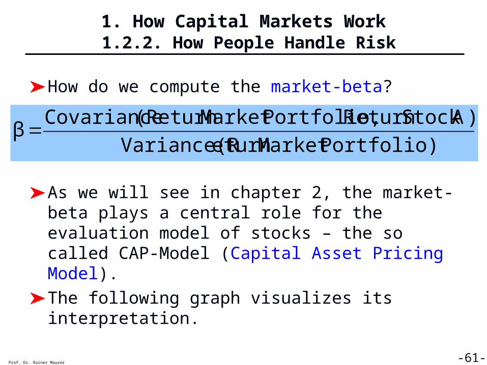
➤ How do we compute the market-beta?
➤ As we will see in chapter 2, the market-beta plays a central role for the evaluation model of stocks – the so called CAP-Model (Capital Asset Pricing Model).
➤ The following graph visualizes its interpretation.
Prof. Dr. Rainer Maurer -61-
Portfolio)MarketeturnVariance(R
)AStocketurnRPortfolio,Market(ReturnCovarianceβ

1. How Capital Markets Work 1.2.2. How People Handle Risk
Prof. Dr. Rainer Maurer -62--50
-40
-30
-20
-10
0
10
20
30
40
50
-50 -40 -30 -20 -10 0 10 20 30 40 50
Return of Stock A
Return of the Market Portfolio
β=1
=> Adding Stock A to the market portfolio does not
change portfolio risk
β=1 => Stock A is as volatile as the market.
“Average β-Stock“
1. How Capital Markets Work 1.2.2. How People Handle Risk
Prof. Dr. Rainer Maurer -63--50
-40
-30
-20
-10
0
10
20
30
40
50
-50 -40 -30 -20 -10 0 10 20 30 40 50
Return of Stock A
Return of the Market Portfolio
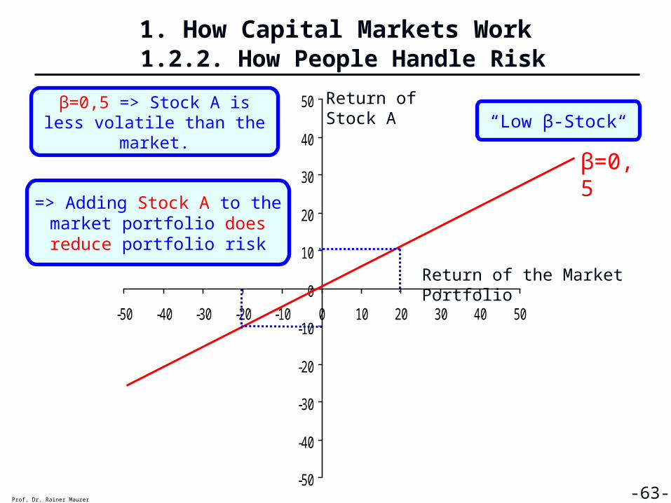
β=0,5
β=0,5 => Stock A is less volatile than the market.
=> Adding Stock A to the market portfolio does reduce
portfolio risk
“Low β-Stock“

1. How Capital Markets Work 1.2.2. How People Handle Risk
Prof. Dr. Rainer Maurer -64--50
-40
-30
-20
-10
0
10
20
30
40
50
-50 -40 -30 -20 -10 0 10 20 30 40 50
Return of Stock A
Return of the Market Portfolio
β=1,5β=1,5 => Stock A is more volatile than the market.
=> Adding Stock A to the market portfolio does increase portfolio risk
“High β-Stock“

1. How Capital Markets Work 1.2.2. How People Handle Risk
Prof. Dr. Rainer Maurer -65-
1. How Capital Markets Work 1.2.2. How People Handle Risk
Prof. Dr. Rainer Maurer -66-

1. How Capital Markets Work 1.2.2. How People Handle Risk
Prof. Dr. Rainer Maurer -67-
1. How Capital Markets Work 1.3.1. The Discounted Cash-Flow Method
1. How Capital Markets Work
1.1. Supply and Demand on Capital Markets
1.1.1. Why People Save
1.1.2. Why People Invest
1.2. Capital Markets and Risk 1.2.1. Why People Don’t Like Risk
1.2.2. How People Handle Risk1.3. Basic Evaluation Techniques for Capital Markets
1.3.1. The Discounted Cash-Flow Method1.3.2. The Internal Rate of Return Method
1.3.3. Risk and Return: The Sharpe Ratio
Prof. Dr. Rainer Maurer -69-
1. How Capital Markets Work 1.3.1. The Discounted Cash-Flow Method
➤ As the next chapter will show, very different kind of assets are traded on capital markets.
➤ Two technical procedures are important for the evaluation of these different assets:
■ Discounted Cash-Flow Method
■ Internal Rate of Return Method
➤ Before we apply these procedures to the various types of assets in the next chapter, we will analyze them in some detail in the following:
➤ We start with the discounted cash-flow method:
Prof. Dr. Rainer Maurer -70-

1. How Capital Markets Work 1.3.1. The Discounted Cash-Flow Method
➤ What do you prefer: 1 € today or 1 € in one year?
➤ The basic idea of the discounted cash-flow method is:
■ Determining the present value of a flow of future payments – either from an investment project or a financial market asset.
■ Technically, payments of different points in time are made comparable by evaluating each payment with a time specific discount factor and adding up these comparable payments to the “present value” of the payment flow.
➤ The following examples show, how this works:
Prof. Dr. Rainer Maurer -71-

1. How Capital Markets Work 1.3.1. The Discounted Cash-Flow Method
Prof. Dr. Rainer Maurer -73-
➤ Discounting a payment flow:
➤ This payment flow with equal annual payments of 100 per year clearly shows that payments further in the future a more discounted than payments closer to the present.
➤ A comparison with the following table shows that a lower discount rate increases the present value:
2008 2009 2010 2011 2012Cash Flow 0 100 100 100 100Discount Rate: 5% *(1,05)^(-1) *(1,05)^(-2) *(1,05)^(-3) *(1,05)^(-4)Present Values 95,2 90,7 86,4 82,3Total Present Value 354,6
Discounting a Cash Flow
2008 2009 2010 2011 2012Cash Flow 0 100 100 100 100Discount Rate: 2% *(1,02)^(-1) *(1,02)^(-2) *(1,02)^(-3) *(1,02)^(-4)Present Values 98,0 96,1 94,2 92,4Total Present Value 380,8
Discounting a Cash Flow
1. How Capital Markets Work 1.3.1. The Discounted Cash-Flow Method
Prof. Dr. Rainer Maurer -74-
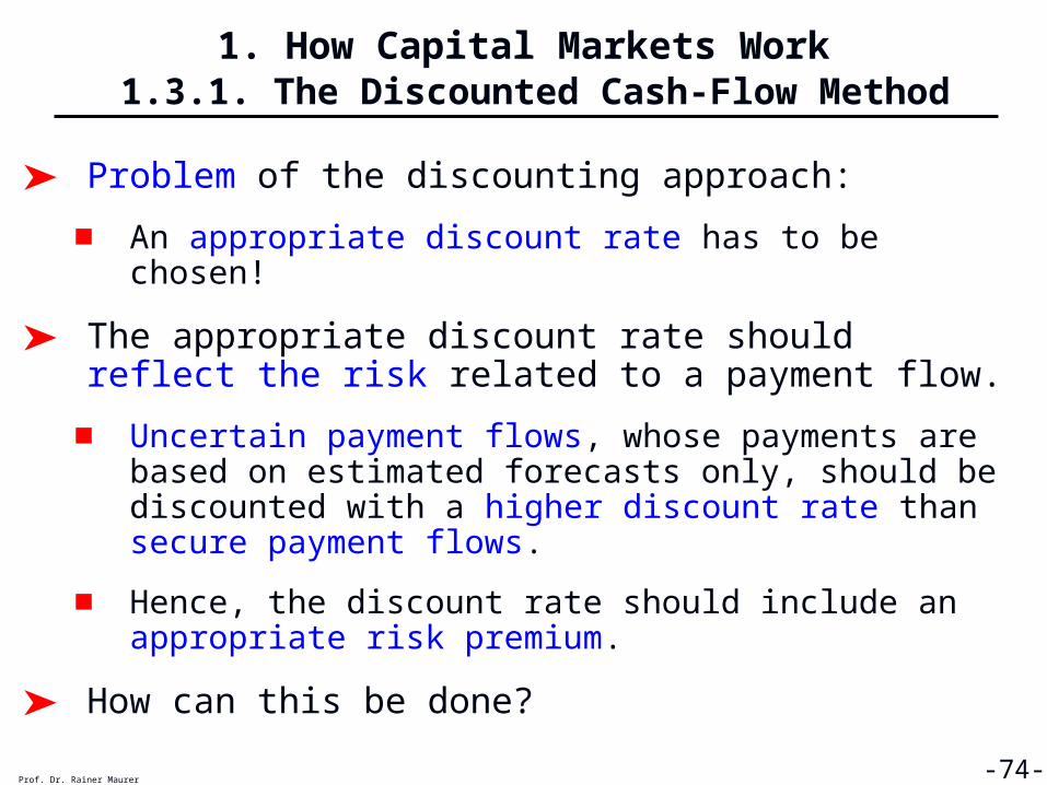
➤ Problem of the discounting approach:
■ An appropriate discount rate has to be chosen!
➤ The appropriate discount rate should reflect the risk related to a payment flow.
■ Uncertain payment flows, whose payments are based on estimated forecasts only, should be discounted with a higher discount rate than secure payment flows.
■ Hence, the discount rate should include an appropriate risk premium.
➤ How can this be done?

1. How Capital Markets Work 1.3.1. The Discounted Cash-Flow Method
➤ How to find the appropriate discount rate?
■ In many cases it is possible to find a market interest rate for a payment flow of the same risk class:
◆ If the payment flow is nearly certain, the market interest rate of a fixed rate security with the same risk structure, for example a bond of a government with high creditworthiness, should be chosen as discount rate.
■ However, for many uncertain payment flows, it is difficult to find a market interest rate of the same risk class.
◆ If the payment flow is uncertain and based on a forecast (for example the dividend payments from a stock company) a market interest rates for exactly the same risk class are hard to find.
◆ In this case, concepts like the Capital Asset Pricing Model (CAPM) can to be employed to calculate an appropriate discount rate. Chapter 2 will show, how this works.
Prof. Dr. Rainer Maurer -75-

1. How Capital Markets Work 1.3.2. The Internal Rate of Return Method
1. How Capital Markets Work1.1. Supply and Demand on Capital Markets
1.1.1. Why People Save1.1.2. Why People Invest
1.2. Capital Markets and Risk 1.2.1. Why People Don’t Like Risk
1.2.2. How People Handle Risk1.3. Basic Evaluation Techniques for Capital Markets
1.3.1. The Discounted Cash-Flow Method1.3.2. The Internal Rate of Return Method1.3.3. Risk and Return: The Sharpe Ratio
Prof. Dr. Rainer Maurer -77-
1. How Capital Markets Work 1.3.2. The Internal Rate of Return Method
Prof. Dr. Rainer Maurer -78-
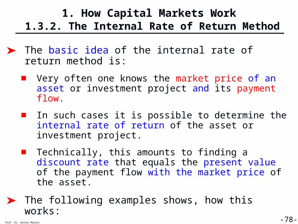
➤ The basic idea of the internal rate of return method is:
■ Very often one knows the market price of an asset or investment project and its payment flow.
■ In such cases it is possible to determine the internal rate of return of the asset or investment project.
■ Technically, this amounts to finding a discount rate that equals the present value of the payment flow with the market price of the asset.
➤ The following examples shows, how this works:

1. How Capital Markets Work 1.3.2. The Internal Rate of Return Method
Prof. Dr. Rainer Maurer -79-
Periods 2009
=> Internal Rate of Return = i = 2,00%
Calculation of the Internal Rate of Return
Market Price of Asset
100
Annual Payments : 102
! 1i1
102
➤ If the payment flow consists of one period only, it is easy to calculate the IRR (=internal rate of return) by hand:
102,1i
02,1001
102i1
i1
102001
t+1

1. How Capital Markets Work 1.3.2. The Internal Rate of Return Method
Prof. Dr. Rainer Maurer -80-
➤ If the payment flow consists of more than one period, for example 5 periods, calculating the IRR implies solving a polynomial of degree 5. This involves the following problem:
■ Formulas for analytical solutions exist only for polynomials lower degree 4.
➤ Therefore, numerical solutions methods must be applied.
➤ One such method is available for Excel (the IKV() Function).
Periods 2009 2010 2011 2012 2013
=> Internal Rate of Return = i = 3,78%
5 102Annual Payments : 3 1 8
Market Price of Asset
100
Calculation of the Internal Rate of Return
1i1
3
2i1
1
3i1
8
4i1
5
5i1
102
!

1. How Capital Markets Work 1.3.2. The Internal Rate of Return Method
Prof. Dr. Rainer Maurer -82-
➤ Consequently, calculating the IRR typically implies the usage of a computer.
➤ If the IRRs of several payment flows are calculated, it is in principle possible to select the payment flow with the highest IRR as the most profitable one.
➤ However, one has to take care of the risk implied by each payment flow!
➤Since an uncertain payment flow is riskier than a certain payment flow, the uncertain flow must offer a risk premium (for people with normal utility function…)
➤One often used measure, which takes care of both return and risk, is the so called Sharpe Ratio, which was proposed by William F. Sharpe (1966).
1. How Capital Markets Work 1.3.3. Risk and Return: The Sharpe Ratio
1. How Capital Markets Work1.1. Supply and Demand on Capital Markets
1.1.1. Why People Save1.1.2. Why People Invest
1.2. Capital Markets and Risk 1.2.1. Why People Don’t Like Risk
1.2.2. How People Handle Risk1.3. Basic Evaluation Techniques for Capital Markets
1.3.1. The Discounted Cash-Flow Method1.3.2. The Internal Rate of Return Method1.3.3. Risk and Return: The Sharpe Ratio
Prof. Dr. Rainer Maurer -83-
1. How Capital Markets Work 1.3.3. Risk and Return: The Sharpe Ratio
Prof. Dr. Rainer Maurer -84-
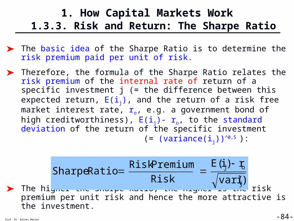
➤ The basic idea of the Sharpe Ratio is to determine the risk premium paid per unit of risk.
➤ Therefore, the formula of the Sharpe Ratio relates the risk premium of the internal rate of return of a specific investment j (= the difference between this expected return, E(ij), and the return of a risk free market interest rate, ro, e.g. a government bond of high creditworthiness), E(ij)- ro, to the standard deviation of the return of the specific investment (= (variance(ij))^0,5 ):
➤ The higher the Sharpe Ratio, the higher is the risk premium per unit risk and hence the more attractive is the investment.
)ivar(
r)i(E
Risk
PremiumRiskRatioSharpe
j
oj

1. How Capital Markets Work 1.3.3. Risk and Return: The Sharpe Ratio
Prof. Dr. Rainer Maurer -85-
➤ Which asset A or B offers the best relation between risk and return? Calculate the Sharp Ratio for a risk free return of 2 %.
Recession Normal BoomReturn of Asset -2% 3% 8%Mean ReturnMean DeviationSquared Mean DeviationVarianceStandard DeviationRisk Free Return 2%Sharpe Ratio
Computing the Sharpe Ratio: Asset A
Recession Normal BoomReturn of Asset -4,0% 4,0% 10,0%Mean ReturnMean DeviationSquared Mean DeviationVarianceStandard DeviationRisk Free Return 2%Sharpe Ratio
Computing the Sharpe Ratio: Asset B

1. How Capital Markets Work 1.3.3. Risk and Return: The Sharpe Ratio
Prof. Dr. Rainer Maurer -86-
➤ Problem with the Sharpe Ratio:
■ The standard deviation of an investment, i.e. the measure for its risk, is typically not known, but has to be estimated based on forecasted future returns. In our above example we simply assumed to know them!
■ For financial market assets, e.g. the return of stocks, such kind of forecasts are typically highly inaccurate.
■ Therefore, very often, the standard deviation of a stock is estimated based on its past returns.
■ Even though such a calculation is easily done and seems to be highly “accurate and plausible”, one has to be aware that the application of such “historic” standard deviations for future investment decisions, implies the “hidden assumption” that the “future” will similar to the “past”.
■ For many kind of stocks, this assumption has proven wrong!

Chapter 1: Questions
You should be able to answer the following questions at the end of this chapter. If you have difficulties in answering a question, discuss this question with me during or at the end of the next lecture or attend my colloquium.
Prof. Dr. Rainer Maurer -88-

Chapter 1: Questions for Review
1. Why can “saving” increase personal utility? Give a graphical and verbal explanation.
2. How does saving behavior affects consumption behavior?
3. If saving increases utility, why do savers demand interest?
4. Why depends the willingness to save positively on the interest rate?
5. What is a “production function”?
6. Explain the motive for investment.
7. Why depends the willingness to invest negatively on the interest rate?
9. What insures the equality of saving and investment in a market equilibrium? Explain your answer based on the a diagram of the capital market.
10. How does an increase in savings supply affect the interest rate?
Prof. Dr. Rainer Maurer -89-

Chapter 1: Questions for Review
11. How does an increase in investment demand affect the interest rate?
12. Explain the meaning of “risk averse” and “risk neutral”.
13. Why are most people risk averse? Give a graphical and verbal explanation.
14. What is a “risk premium”?
15. Why do people demand a risk premium?
16. What is “hedging”?
17. What property must two stocks have to be a “perfect hedge”?
18. Is it possible to hedge risk with two stocks, if there return is positively correlated?
19. Why are perfect hedges rare?
20. What is a “normal hedge”?
21. How do you explain that so many stocks are “normal hedges”?
Prof. Dr. Rainer Maurer -90-

Chapter 1: Questions for Review
22. Calculate the variances and the correlation coefficient of the following stocks. Can they be used to hedge each other?
23. Calculate the variances and the correlation coefficient of the following stocks. Can they be used to hedge each other?
24. What is the “market-beta”?
25. What is meant by “low beta stock” and “high beta stock”?
Prof. Dr. Rainer Maurer -91-
Stock 2002 2003 2004 2005 2006 2007 Variance Corr. Coeff.Stock A 160 130 150 80 70 180Stock B 30 60 40 110 120 10Sum / 2
Stock 2002 2003 2004 2005 2006 2007 Variance Corr. Coeff.Stock A 110 100 60 130 110 170Stock B 100 90 50 120 100 160Sum / 2

Chapter 1: Questions for Review
26. Give a verbal explanation of the discounted cash flow and the internal rate of return method.
Prof. Dr. Rainer Maurer -92-
2008 2009 2010 2011 2012Cash Flow 0 100 100 100 100Discount Rate: 4%Present ValuesTotal Present Value
Discounting a Cash Flow
27. Which criteria should an appropriate discount rate fulfill?
28. What is the definition of the Sharpe Ratio?
29. Give a verbal interpretation of the Sharpe Ratio.
30. What are the two major criteria for an investment decision?

Chapter 1: Questions for Review
31. What asset is the most attractive? Base your decision on the Sharpe Ratio.
Prof. Dr. Rainer Maurer -93-
Recession Normal BoomReturn of Asset -1,0% 4,0% 10,0%Mean ReturnMean DeviationSquared Mean DeviationVarianceStandard DeviationRisk Free Return 2%Sharpe Ratio
Computing the Sharpe Ratio: Asset C
Recession Normal BoomReturn of Asset 0,0% 3,5% 9,0%Mean ReturnMean DeviationSquared Mean DeviationVarianceStandard DeviationRisk Free Return 3%Sharpe Ratio
Computing the Sharpe Ratio: Asset D

Prof. Dr. Rainer Maurer -94-
Portfolio Theory