international capital flows and development...
TRANSCRIPT
1
International Capital Flows and Development:
Financial Openness Matters
Dennis Reinhardt, Luca Antonio Ricci and Thierry Tressel1
March 2013
Abstract
Does capital flow from rich to poor countries? We revisit the Lucas paradox to account
for the role of capital account openness. We find that, when accounting for such
openness, the prediction of the neoclassical theory is empirically confirmed: among
financially open economies, less developed countries tend to experience net capital
inflows and more developed countries tend to experience net capital outflows. The
results holds also when taking into account private flows, institutions, and numerous
controls. We also show that reserve intervention has an effect on the current account
only in financially open economies.
Keywords: Lucas paradox, capital flows, financial openness, economic development
JEL Classification: F21, F36, O4
1 Dennis Reinhardt is at the Bank of England; the first version of the paper was written while he was affiliated to the
Graduate Institute of International and Development Studies (Geneva) and the Study Center Gerzensee; email:
[email protected]. Luca Antonio Ricci and Thierry Tressel are at the International Monetary
Fund; emails: [email protected], [email protected]. We are thankful to Governor DeLisle Worrell, Stjin Claessens, Tito
Cordella, Neil Ericcson, Atish R. Ghosh, Eduardo Levy Yeyati, Gian Maria Milesi-Ferretti, Rahul Mukherjee, Andy
Neumeyer, Jonathan Ostry, Rodney Ramcharan, Ugo Panizza, Andy Powell, Cédric Tille and anonymous referees for
useful comments as well as participants of the 2012 DIW conference on “Intra-European Imbalances, Global
Imbalances, International Banking, and International Financial Stability”, and in the 2012 (VIII) Workshop of the Latin
American Financial Network (LFN). This paper is a revised version of IMF Working Paper No. 10/235. Any views
expressed are solely those of the author(s) and so cannot be taken to represent those of the IMF, the Bank of
England, or the policies of these institutions. This paper should therefore not be reported as representing the views
of the Bank of England or members of the Monetary Policy Committee or Financial Policy Committee.

2
1. Introduction
This paper revisits the Lucas paradox by quantifying empirically the relevance of a specific
set of policies—restrictions on international capital flows—in shaping the patterns of capital
movements at various stages of economic development. The determinants of the direction of
capital flows, and their relation with economic development, constitute an important topic in
open economy macroeconomics. The study is particularly relevant in the current context, where
the size and direction of capital flows have been at the epicenter of the debate on global
imbalances and remain relevant in the aftermath of the global financial crisis. Indeed, it remains
unclear, empirically, whether (and which) policies can result in capital flowing “uphill”.
The premise is the classic paper in which Lucas (1990) remarked that too little capital flows
from rich to poor countries, relative to the prediction of the standard neoclassical model (“Lucas’
paradox”). According to neoclassical theory, when countries have access to similar technologies
and produce similar goods, new investment—and therefore international net capital inflows—
should take place more extensively in poorer countries with lower stocks of capital per capita
and therefore a higher marginal product of capital.
A large theoretical and empirical literature has flourished to provide solutions to the
"Lucas paradox", by extending the basic neoclassical model to encompass additional factors. A
first group of factors include differences in technologies, factors of production, and government
policies. A second group of factors relate to the role of institutions and capital market
imperfections, encompassing the quality of enforcement of private contracts, asymmetric
information and moral hazard, risks of expropriation, and sovereign default.
In this paper, we step back and show that the ‘failure’ of the neoclassical model to predict
international capital flows can also be explained by a violation of one of the model’s key
underlying assumptions: capital can flow freely across countries.
Specifically, we find that the prediction of the standard neoclassical theory holds only
when taking into account the degree of capital account openness, conditional on a set of
fundamentals. Among countries with an open capital account, richer countries tend to
experience net capital outflows, while poorer countries tend to experience net capital inflows. In
contrast, in countries with closed capital account, there appears to be no systematic relationship
between the level of economic development and net capital flows. The results imply that capital

3
account restrictions must have been effective in constraining capital flows when they were in
place: rich countries liberalizing their capital account should experience net capital outflows and
poor countries net capital inflows.
In contrast to the recent literature that has sometimes emphasized long-term
determinants of cross-sectional differences in capital flows, we focus mainly on the impact of
capital account liberalization on capital flows over time. This approach is the consequence of a
simple observation: as Figure 1 illustrates, policies related to capital account openness have
dramatically evolved during the past thirty years.2 At the time Robert Lucas was writing his
paper, many developing countries still had significant capital account restrictions in place.
However, since then, countries across all income groups have progressively liberalized capital
movements. High income countries (those that still had restrictions in place) initiated the
process in the 1980s; by the early 2000s, cross-border capital was flowing freely among
advanced economies. Emerging markets followed the same process of liberalization, but with a
lag. Many restrictions were removed in the early 1990s, sometimes to prepare entry in the OECD
(as was the case for Korea and Mexico, see IMF, 2003), or under the auspice of the International
Monetary Fund. Liberalization of capital movements started at a later stage in lower income
countries, mostly in the second half of the 1990s (some moderate restrictions have remained in
place until now). We show that this liberalization process was associated with significant changes
in the patterns of capital flows across countries at different income levels.
Our findings have important policy implications. Policies related to the capital account
create externalities in the international monetary system by sustaining large current account
imbalances. Our results suggest that liberalizing the capital account would significantly reduce
these distortions and allow capital to flow into the fast growing emerging market surplus
countries.
Our paper also offers useful empirical implications: because of a global trend towards
capital account liberalization, and as more data becomes available over time, empirical studies
will be less and less likely to detect the Lucas puzzle for the average country.
2 The measure of capital account openness is an updated index from Quinn (1997). See appendix for more details.

4
The paper proceeds as follows. Section 2 provides an overview of the related literature.
Section 3 presents the data and simple stylized facts. Empirical strategy and results are in section
4, and section 5 concludes.
2. Literature
While a large literature has provided elements of answers to the Lucas paradox, there are,
to date, few empirical studies assessing the role of capital account restrictions in shaping capital
flows from an economic development point of view.
Empirical studies of the Lucas paradox typically show how relaxing one (or several)
assumptions of the basic neoclassical model helps explain capital flows from rich to poor
countries. Differences in human capital (Lucas, 1990), in the risk of sovereign default (Reinhart
and Rogoff, 2004b), in capacity to use technologies (Eichengreen, 2003), and in institutional
quality (Alfaro, Kalemli-Ozcan and Volosovych, 2008) seem to be relevant for the direction of
cross-border capital flows.3 The emphasis on institutional quality is the natural consequence of a
body of work showing that social infrastructure, which includes government policies and
institutional structure (Hall and Jones, 1999), and some specific institutional characteristics, such
as the protection against the risks of expropriation (Acemoglu and Johnson, 2005), have first
order effects on long-run economic performance by affecting investment and total factor
productivity. Obstfeld and Taylor (2005) showed that during the 1990s, net capital flows to poor
countries remained relatively small, while gross capital flows, in general, were large, in particular
among advanced economies. This, they argued, was evidence that portfolio diversification, not
development finance, was the main factor driving financial integration. Our results suggest that
net development finance was an important driver of international capital flows among financially
open economies.
Our paper is related to recent work by Alfaro, Kalemli-Ozcan and Volosovych (2011). They
disaggregate international capital flows into their private and public components and find that
international capital flows net of sovereign to sovereign borrowing in the form of debt or aid are
3 Alfaro et al. (2008) include a measure of capital account restrictions (based on the IMF Annual Report on Exchange
Arrangements and Exchange Restrictions) among the set of control variables. They find that restrictions have a
significant and negative bearing on gross capital inflows, but do not look at net capital flows or the interaction with
the level of development.

5
positively correlated with growth. As aid flows form the biggest part of capital flows going into
poorer countries, they find evidence for a Lucas paradox in a sample that contains both
financially open and closed economies when accounting for these flows. We find consistent
evidence by showing that (mainly private) capital flows downhill among financially open
economies.4
Another relevant contribution was made by Kalemli-Ozcan, Reshef, Sorensen and Yosha
(2008), who focus on interstate capital flows within the US, and show that the standard model
explains capital flows between US states well. They suggest that frictions in national borders may
explain the failure of the neoclassical model in accounting for the direction of capital flows. As
there are no restrictions to capital flows within states, this result is consistent with ours.
The importance of financial frictions in international capital flows was recently highlighted
by Gourinchas and Jeanne (2009) who showed that, among developing countries, capital flows
more to countries that do invest and grow less. By calibrating a neoclassical model, they find that
a wedge affecting saving decision may explain this "allocation puzzle". Reinhardt (2010) provides
a sectoral approach to the "allocation puzzle" and shows that services sector FDI flows into fast-
growing emerging markets, especially if they are financially open. Compared to us, he however
focuses on growth (Allocation puzzle) instead of income (Lucas paradox) and employs a sample
that includes only emerging economies. Verdier (2008) shows that, in presence of an
international borrowing constraint and complementarity between domestic and foreign capital
in production, foreign debt rises with domestic savings, a prediction consistent with data on
capital flows. Some papers, motivated by China's experience and global imbalances, have
emphasized that the interaction of borrowing constraints with precautionary savings, with a
process of reform, or with a shortage of financial assets is associated with fast economic growth
and a current account surplus (Sandri, 2010; Song, Storesletten and Zilibotti, 2009; Buera and
Shin, 2009; Caballero, Fahri and Gourinchas, 2008; Mendoza Quadrini Rios-Rull, 2008).
A novel perspective on the paradox of capital flows was provided by Caselli and Feyrer
(2007) who showed that, once properly measuring the share of income accruing to physical
capital and accounting for the relative price of capital goods, the marginal product of capital
4 A related paper (Lowe, Papageorgiou, and Perez-Sebastian, 2012) shows that different marginal productivities of
capital for public and private investment can offer an alternative explanation of the Lucas’ puzzle.

6
(MPK) is quite similar across countries. In a related contribution, Causa et al. (2006) argue that
capital-output ratios are similar across countries once market prices are used to calculate the
market value of the productivity of physical capital. However, there remains some skepticism
regarding evidence suggesting equalization of aggregate MPK, in part arising from the
microeconomic evidence that there are, within countries, substantial differences in productivity
and MPK between firms (Hsieh and Klenow, 2009; Restuccia and Rogerson, 2008; Alfaro,
Charlton and Kanczuk, 2007). Chirinko and Malik (2012) argue that, when adjustment costs and
capital depreciation are taken into account and parameterized, the MPK differentials between
poor and rich countries are significantly higher than implied by traditional estimates.
Our paper is also related to one of the major puzzles of international finance, such as the
high correlation between savings and investment (The Feldstein-Horioka puzzle). In line with our
results, recent contributions showed that the process of economic integration (in particular
monetary and financial liberalization) among European countries resulted in capital flows
towards relatively poorer countries, resulting in a declining correlation of savings with
investment (Coeurdacier and Martin, 2009; Lane and Milesi-Ferretti, 2008; and Blanchard and
Giavazzi, 2002). Lewis (1996) shows that international capital market restrictions are needed to
find evidence for international risk-sharing. Compared to her paper, we control for determinants
of capital flows and focus on the impact of differences in development on capital flows rather
than shocks to output growth. We find that capital market restrictions are sufficient in resolving
the puzzle of poor-to-rich country capital flows, conditional on a set of fundamentals.
There exists, to date, no strong consensus on the effectiveness of capital controls (see
Edwards, 1999, for a survey; see also Edwards and Rigobon, 2009; Forbes, 2007; Edison and
Reinhart, 2001). While they seem effective when extensive restrictions are in place, re-imposing
some restrictions seem to affect mainly the composition of inflows rather than the aggregate
volume of inflows (see Ostry et al., 2010, for a recent study). For example, in the case of Chile
and Colombia, capital controls seem to have tilted the composition of capital flows towards less
volatile types of flows (De Gregorio, Edwards and Valdes, 2000; Cardenas and Barrera, 1997).
Our paper studies the removal of pervasive capital controls rather than the impact of their re-
introduction for potential prudential concerns.

7
Finally, our paper is also related to papers analyzing the medium-term determinants of
current accounts across countries to characterize net capital inflows. Chinn and Prasad (2003)
show that medium-term fundamentals such as fiscal policy, demographics, initial net foreign
assets and relative income per capita are relevant determinants of current accounts in a large
sample of countries. Other papers have stressed the role of financial development, financial
crisis or institutional variables (Chinn and Ito, 2007; Gruber and Kamin, 2007, 2008; Chinn,
Eichengreen, and Ito (2011)), or have restricted the analysis to low income countries
(Christiansen, Prati, Ricci and Tressel, 2009).
3. Data
3.1 Data and Descriptive Statistics
We mainly employ the extensive dataset assembled by Christiansen et al. (2009)
containing information on the current account balance, relative income, financial openness data
and various control variables for 110 countries with populations above one million over the
period 1980-2006. A description of all variables, data sources and a list of all countries are
provided in the Appendix. Most of our analysis is based on a panel of non-overlapping five-year
averages over the period 1982-2006.5 Summary statistics are provided in table A1. Correlations
between the main variables are in tables A2 and A3 (for the within transformed variables).
The dependent variable in most of the analysis is the current account balance relative to
GDP. This treats errors and omissions as unreported capital flows and includes flows in reserve
assets. To distinguish official from private capital flows, we also use two alternative measures of
total net outflows. First, we add concessional loans to the current account balance, because they
are not determined by the MPK, but are classified in the financial account of the Balance of
Payment. Indeed, concessional loans can finance larger imports—and hence worsen the current
account deficit—than would otherwise be possible in their absence. We add only concessional
loans rather than total aid flows from the current account because grants (the second
5 We take averages of the dependent variable and all the controls except for relative income and net foreign assets,
for which we employ the initial value (i.e. the value for the year preceding the 5-year average). If the first or the last
year is missing within the 5-year time frame, we replace the 5-year average with the corresponding 4-year average.

8
component of total aid flows) are already accounted for in the current account. Hence, if all
official grants are spent on imports, we should find no correlation between the current account
and grants. If however part of grants are not spent on imports and are saved instead, we should
observe a positive correlation between the current account and grants (Christiansen et al.,
2009). Second, we also derive an alternative measure of total net outflows by subtracting flows
in reserve assets from the current account balance. Third, we also provide evidence by looking at
net private capital flows.
Our main measure of capital account openness is the index of capital account liberalization
constructed by Quinn (1997) updated to 2006. This is a de jure index measuring capital account
restrictions, and normalized between 0 and 1 (representing fully closed and fully open regime,
respectively); it is a step function that increases in steps of 0.125 (there are hence 9 possible
values). It is constructed from information contained in the IMF’s Annual Report on Exchange
Arrangement and Exchange Restrictions (AREAER). This index has several advantages (see Quinn,
Schindler, and Toyoda, 2011) including a wide sample availability (122 countries), robustness to
structural breaks, and its exclusive focus on capital account restrictions (another widely used
measure by Chinn and Ito (2007) includes also financial restrictions on the current account). We
show below robustness of the results to employing the Chinn and Ito index.
3.2 A First Look at Data
This section shows that the main results are visible even with simple cursory look at the
data. Figure 2 displays the median current account to GDP by income groups during 1982-2006.
For each five year period, countries are grouped into a closed capital account group (respectively
an open capital account group) if the degree of initial capital account openness during the period
is below or on (respectively above) the median openness (Panel A). Panel B shows the same
calculations for a stricter definition of openness, i.e. above the next highest percentile of capital
account openness following the median (i.e. above the 62th percentile) for the complete
period.6 For either panel, there is a clear difference between the closed and open set of
observations.
6 For high income countries there are only 15 out of 115 observations which are below or equal to the sample
median. To ensure that there are enough relatively “closed” countries, for this Figure, we classify a high income
countries into the open group if its level of initial openness is above the median of openness for high income
9
Among countries with a relatively open capital account, the cross-section of current
accounts seem, on average, consistent with the hypothesis that capital flows from rich to poor
countries. Advanced countries seem to have experienced net capital outflows at the median. All
other groups of countries experienced median net capital inflows with low income countries
receiving more capital inflows than middle income countries. In contrast, among countries with a
relatively closed capital account, there is no evidence of a positive correlation between the
current account and the level of development. In particular, even the median observation for
high income countries seems to have experienced net capital inflows.
As discussed in the previous section, the right column offers an alternative calculation
netting out from the current account the financing effect of concessional loans (given their
extensive grant component). The results are even stronger.
When focusing on a more restricted group of very open economies in Panel B (i.e. using
the index value of the initial openness index following the median), results appear even more
consistent still with the hypothesis of downhill capital flows. Accounting for concessional loans,
the difference in annual net capital flows between middle income countries and high income
countries was about 3 percentage points of GDP; the difference in annual net flows between
middle income countries and low income countries was about 2 percentage points of GDP.
Finally, Tables A2 and A3 report simple bilateral correlations before and after netting out
the country specific mean. Interestingly, while the correlation between GDP per capita and the
capital account index is high (0.53) before removing country specific means, it becomes
insignificant after removing these time effects (-0.13). This suggests that our main results, arising
from the interaction term between these two variables, is not the result of the high correlation
between the two variables interacted (indeed, in Tables 4 we will show that our result is not
proxying for nonlinearities in the effect of development).
4. Current Account, Development, and Financial Openness
This section contains the main results.
countries (0.75); this splits the sample of high income countries roughly in half (i.e. 55 observations in the closed
and 75 observations in the open group).

10
We outline the empirical approach in section 4.1 and discuss the results in section 4.2. To
assess the dynamics of the effect of capital account liberalization on the current account, we
proceed with an event study in section 4.3.
4.1 Empirical Approach
The neoclassical model – assuming an open capital account– predicts that private capital
should flow from more developed to less developed economies which have a lower per capita
stock of capital and should therefore have a higher MPK (Lucas, 1990). Hence, it predicts a
positive correlation between the current account and GDP per capita, assuming a common
constant return technology and Hicks-neutral productivity parameter. With an open capital
account, the dynamics of the net foreign asset position is determined by equalization of the
marginal utility of consumption across periods and equalization of the MPK across countries, and
we observe that:
_ · where 0
Capital account restrictions could, if effective, alter the relationship between private
capital flows and GDP per capita even if other assumptions of the neoclassical model are
satisfied. With controls on cross-border capital flows in place, countries may be able to prevent
capital from flowing in even if they enjoy a higher MPK. For this to be possible, the policy maker
must be able to affect the path of consumption and savings and therefore the current account
and real exchange rate path, independently from the MPK. Jeanne (2012) shows theoretically
that, when the capital account is closed, this can indeed be achieved under certain conditions. If
for instance, the government is the only agent with access to foreign financial assets (held for
instance in the form of international reserves), and only domestic private agents can hold
government debt, the government can determine the path of net foreign assets, hence the
current account (equal to the change in the net foreign assets, net of valuation gains/losses and
capital account transfers), and therefore the trade balance. Specifically, the rate of return on
domestic capital is delinked from the international interest rate, and determined by the supply
of government debt. To the extent that government policy is uncorrelated with the level of
development conditional on a closed capital account, the relationship between net capital flows
and the current account will become insignificant. For example, to raise the current account
11
balance, the government can force domestic saving by increasing the supply of government debt
to purchase foreign asset.7 Hence, for countries with a closed capital account, the following
relationship will be observed:
· , where 0
Consider a normalized index of capital account restriction, where a higher corresponds to a
more open capital account, or a higher probability that capital will flow unimpeded. Conversely,
a lower index corresponds to a country in which the probability that capital flows will be affected
by government policies, instead of being affected by private investment and saving decisions
reflecting among others differences between the country MPK and the international rate of
return on capital. The observed relationship between net inflows and per capita GDP will thus be
approximated by:
1 ·
Theory then implies that the effect of removing capital account restrictions depends on the level
of development. According to Jeanne (2012), as restrictions on the capital account are removed
the real exchange rate (and therefore the current account) should adjust to its equilibrium level.
This implies, that, assuming cross-country differences of MPK positively correlated with per
capita stock of capital (and therefore GDP per capita), the real exchange should appreciate (resp.
depreciate) in less (respectively more) developed countries. Thus, capital should flow in poorer
countries and flow out of richer countries as capital account restrictions are removed.
This discussion suggests that it is appropriate to examine how financial openness impacts
the relation between net capital outflows and relative income by including an interaction term
between financial openness and income in an econometric analysis of net capital flows.
Specifically, we estimate the following equation:
OutflowsGDP ,
α β GDPPC , β CAL , β CAL , · GDPPC , Β X , ε
where the dependent variable O f
GDPis net capital outflows (relative to GDP), GDPPC ,
refers to the log of GDP per capita relative to the U.S. (in PPP), CAL , captures the level of
7 See also Prati and Tressel (2006) for a model with monetary policy and closed capital account where a similar
result holds.

12
capital account openness and ε is the error term.8 Net capital outflows are proxied by the
current account balance in most specifications, but occasionally by the three alternative proxies
described in section 3.1.
To focus on the time-dimension of the data while smoothing out the impact of short-run
fluctuations, we use a panel of non-overlapping five-year averages (as in Chinn and Prasad, 2003)
over the period 1982-2006; there are 5 time observations for most countries. GDPPC , and
CAL , are in initial terms, where “initial” indicates the year preceding the 5-year average.
GDPPC , is in initial terms to make sure that we do not capture a potential impact of capital
inflows on GDP per capita. We regard capital account liberalization as a policy choice
uncorrelated with current account developments in the following period, and thus also express it
in initial terms (to match the timing of our per capita income variable).
Our main coefficients of interest are β and β . If β is significantly positive, richer
(respectively poorer) countries experience less (respectively more) capital inflows if they are
financially open; if β + β is significantly bigger than zero, countries with a fully open capital
account display the positive relation between income and capital outflows that is predicted by
the neoclassical model; if β is not significant or significantly negative, countries with a fully
closed capital account do not display the expected neoclassical pattern of capital flows.
The vector of controls X contains control variables which were found to be important in
the literature (see for example Chinn and Prasad, 2003, and Chinn and Ito, 2007), such as the
fiscal balance, demographic variables (the old age dependency ratio, population growth), the
initial net foreign asset position, the oil trade balance, and real per capita GDP growth. We add
an index for the terms of trade in goods and services as well as Aid flows to GDP as controls,
because (i) these variables have been found to be important current account determinants for
low income countries (Christiansen et. al (2009)) and because (ii) Alfaro et al. (2011) point to the
importance of accounting for official aid flows when explaining patterns of international capital
flows. Terms of trade can be included only in the fixed effect specification due to the index
8 Agion et al. (2005) also use GDP per capita relative to the US level as a proxy for the technology gap with the
leader. In this sense, the variable captures the differences in MPK that may arise from differences in the stock of
capital and technology gaps.

13
nature of this variable. Throughout the paper we refer to this set of variables as “standard”
controls.
Our preferred panel results include country fixed effects as it is likely that slow-moving
unobservable variables have an impact on the main coefficients of interest. However, following
many studies in the literature on medium-term determinants of the current account (e.g. Chinn
and Prasad, 2003, and Gruber and Kamin, 2007), we also present results from OLS regressions on
the pooled data that are based on both the time- and the cross-sectional dimension of the data.
We also present results for a panel specification where we split the capital account
liberalization variable into a dummy for financially open and closed observations. For this
purpose, we define a dummy variable that is one if a country’s level of financial openness is
above a certain percentile of the whole-sample distribution of financial openness. We chose to
employ a spline search procedure to find the optimal percentile – i.e. the one that maximizes the
within R2 of the regression including fixed effects. The dummy is then used to replace CAL in
the basic specification above. Further details are given in the Appendix; in the results section
below we refer to this specification as the “spline specification”.
Finally, we assess the time horizon relevant to evaluating the current account to GDP
relationship using an event study type setup. For this purpose we define an liberalization event
as a marked increase in the index of capital account openness and assess the current account to
GDP ratio (including or excluding concessional loans) for the different income groups in the year
of liberalization and in the two 5-year intervals after the year of liberalization (more details can
be found in section 4.3).
4.2 Regression Results
As a first visual test we split the sample in open and closed observations. Figure 3 presents
the result of a regression of the current account on log initial income relative to the US, the
standard determinants and country fixed effects for observations related to closed capital
account (an index value of initial openness below or on the median) in the upper panel; the
regression for observations related to an open capital account (i.e. index values above the
sample median) is in the lower panel. There is a clear difference between the two groups:
current accounts and initial income appear to be positively related only for the case of open

14
capital account. This suggests that the prediction of the neoclassical growth model may only be
confirmed for countries with open capital accounts. In the remainder, we offer tests of this
hypothesis.
We present pooled and fixed effect regressions in Table 1. In columns 1-2, we find,
conditional on standard determinants and aid flows to GDP, that per-capita income and capital
flows are statistically unrelated—a finding that reflects the Lucas paradox as it is inconsistent
with the standard neoclassical theory.
This is in line with the findings of Alfaro et al. (2011) that provide evidence of a Lucas
paradox in a regression that accounts for aid flows. Chinn et al. (2011), updating earlier studies
on the medium-run determinant of the current account, find in a similar regression a positive
coefficient on relative income, but they do not control for aid flows.
Aid flows to GDP enter negatively and strongly significantly suggesting that, in low income
countries, a large proportion of capital flows are official flows. These capital flows are not
determined by the private rate of return on capital, but by other considerations such as social
needs and humanitarian assistance. Hence we may observe lower current account balances in
some low income countries, not because private capital flows in, but because they receive aid
inflows. Coefficients on other variables are roughly similar in size and significance to Chinn et al.
(2011)’s findings for the 1970-2008 period.
The coefficient on the degree of capital account openness is negatively (though statistically
not significant) correlated with the current account to GDP ratio suggesting that – on average–
controls have been more binding in countries that want to borrow.
Next, we include in columns 3 and 4 an interaction term with the initial level of GDP. The
rationale for including an interaction term is discussed in section 4.1. We find that the
correlation between the current account and the level of development depends strongly on the
degree of capital account openness.
Indeed, in countries with strong capital account restrictions (for which the capital account
index is close to zero), there is no significant positive correlation between the initial level of
development and the current account, as the coefficient on the income per capita in column (4)
variable is not significantly different from zero (in column 3 it is negative, which is even the

15
opposite of the neoclassical theory prediction; however, this regression is less reliable as it does
not include fixed effects).
But for countries with few capital account restrictions (index close to one), we find that the
effect of income for countries with open capital account (offered by the sum of the first and
third coefficient, whose p-value is reported at the bottom of the table)9 is positive and
significant. The prediction of the standard neoclassical theory (capital should flow from more
developed to less developed countries) can be confirmed only for countries with open capital
accounts.
The estimated coefficients for the preferred fixed effect specification (column 4) imply
that, a lower middle income country at 10 percent of the US income level with an open capital
account runs a current account that is 5.2 percentage points of GDP lower than a country with
an income level at 50 percent of the US level, after controlling for various determinants of the
current account.10
The results can also be interpreted from a different perspective. We find evidence that,
when controlling for standard determinants of the current account, the correlation between the
current account and the degree of capital account openness is negative for poor countries and
positive for rich countries. This suggests that capital account restrictions tend to reduce on
average the volume of net capital inflows in poor countries, and of outflows in rich countries.
Based on the within country coefficient of column 4, a middle income country with income per
capita at 10 percent of the US level (such as China, Egypt, or Indonesia in 2004) would
experience an additional annual net capital inflow of about 2.2 percent of GDP annually
following a complete opening of the capital account. At the other end of the development
spectrum, an advanced country with income per capita at 90 percent of the US level would
experience additional annual capital outflows of 4.7 percent of GDP after a complete opening up
of the capital account.
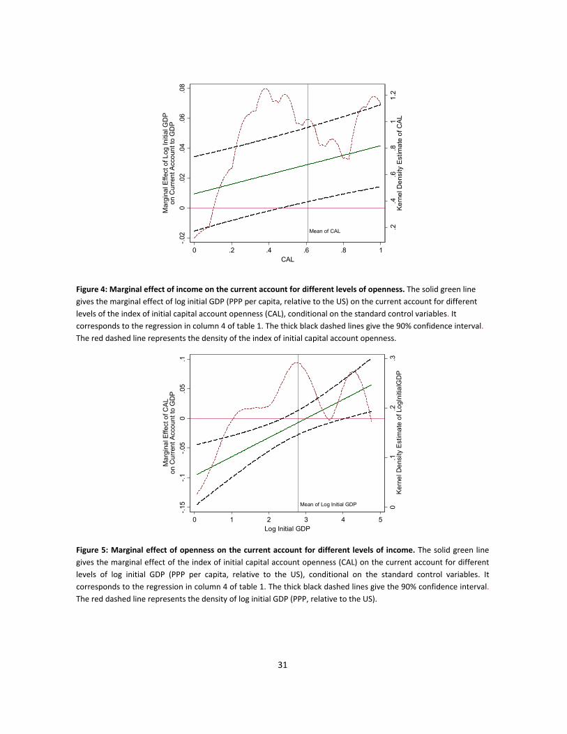
Figure 4 illustrates the relationship between the level of development and the current
account for various degrees of capital account openness. Our quantification implies that the
relationship becomes significantly positive for an index of financial openness above 0.5. The red
9 The F test is the following: coefficient (log GDP per capita) + coefficient (log Initial GDP per capita * Capital account
index)=0 for capital account index=1. 10
Portugal or Slovenia had PPP adjusted income levels at 50 percent of US level in 2000.

16
dashed line in Figure 4 represents the density of capital account openness and suggests that
there are two groups of open and closed economies for which the marginal effect of income on
the current account differs markedly.
Figure 5 illustrates the relationship between capital account openness and the current
account for various degrees of income. Our quantification implies that the relationship becomes
positive for a level of log initial GDP of almost 3 which corresponds to a level of initial relative
GDP to the US of about 20% (which in turn corresponds to the 62th percentile of the distribution
of initial relative GDP to the US).
This result suggests that capital inflows are undistorted only if the capital account is
sufficiently free of restrictions. To capture these possible threshold effects, we create various [0-
1] dummy variables for "open capital accounts" based on different thresholds for openness; we
then interact the dummy with the initial level of development and search for the dummy (and
hence the threshold) that would maximize the R2 (see appendix for a deeper description of this
spline procedure). According to the best threshold, countries are in the open group if their index
value of initial openness exceeds 0.5 (which coincides with the full sample median). Table 2
reports the results from the spline specification which are similar to the basic specification in
Table 1. For the group of financially closed economies, we find evidence for a Lucas paradox:
initial GPD and the current account are statistically unrelated. Conversely, for the group of
financially open economies we do not find evidence for a Lucas paradox: once capital is allowed
to flow freely, it flows according to the prediction of the neoclassical model.
Table 3 explores the results using different thresholds: we find that the interaction term
and the effect of income on the current account for the financially open group becomes weaker
the more closed observations we include in the “open” group.
Robustness
Tables 4 and 5 offer robustness checks. In table 4.1 and 4.2 (for the basic and the spline
specification, respectively), we check that our findings are robust to adding various control
variables to our standard controls. First, in columns 1-6 we include alternative or additional
controls that can be expected to have a impact on the current account. Second in columns 7-9
we inspect the role of institutions and nonlinearities in development, and check that our effect

17
from capital account liberalization is not simply proxying for these factors. Third, in columns 10-
11, we analyze the role of reserve accumulation. Finally in column 12 we include all significant
additional regressors.
Column 1 of Tables 4.1 and 4.2 splits aid flows to GDP into its two components,
concessional loans to GDP and net grants to GDP. Our main results are not affected. We also find
that net grants, a component of the current account, enter insignificantly (suggesting that they
are fully spent on imports, a result roughly in line with Christiansen et al., 2009, who find a
coefficient of 0.2, which is significant at the 10% level). Conversely, concessional loans are
strongly negatively associated with the current account balance.
Domestic financial development may affect the current account. The effect, however, is
theoretically ambiguous: a deeper and more efficient financial system may stimulate savings and
therefore raise the current account, but it may also boost investment and therefore worsen the
current account. As a proxy we use the ratio of private credit to GDP (column 2), a standard
measure of financial development, which appears to negatively affect the current account. We
also find that domestic credit growth is significantly negative, possibly capturing excessive
borrowing during financial booms (column 3), but does not affect our results.
Changes to a country’s exchange rate regime may have an impact on capital flows:
however, the index developed by Reinhart and Rogoff (2004a) is not significant (column 4). A
number of countries experienced banking crisis during the sample period, which may be
associated with reversals in the current account. The coefficient on the variable that measures
the incidence of banking crisis is positive as expected, however not significant (column 5), and
again leaves our results unaffected.
Human capital is an important determinant of the rate of return on capital, and therefore
could affect capital flows. However, a standard measure of human capital (years of schooling) is
not significant (column 6) and our results hold.
As capital account openness is correlated with institutions and the level of development,
one general concern is that the main result on the role of capital account openness in shaping
the effect of the level of development is simply due to such openness proxying for the role of
institutions or for nonlinearities in the effect of development. We therefore now show that our
results hold independently of these possible factors.

18
A recent literature has argued that institutions have first order effects on the development
process. In particular, the quality of property rights affects economic growth and financial
development (Acemoglu and Johnson, 2005), and capital flows (Alfaro et al., 2008; Faria and
Mauro, 2009). We consider a standard proxy of property rights (a de facto measure of the
perception of the quality of institutions from the International Country Risk Guide, ICRG), and
find that better institutions (a higher value of the index) are indeed, as in Alfaro et al., 2008,
associated with lower current accounts (column 7). Our results are however not affected. When
we include also an interaction term between our measure of initial GDP and institutions to run a
horse race between capital openness interaction and institution interaction (column 8), we find
that the institution interaction is not significant while our results broadly hold (the p-value of the
GDP coefficient for open capital account is 0.047 in the main specification and borderline at
0.116 in the less preferred specification). This indicates that the role of financial openness is
robust to controlling for the role of institutions.
As documented in Fogli and Perri (2006), the second order terms of economic activity
affect the current account. We therefore add the square of log initial GDP to the baseline
regression (column 9), but find that this does not alter the results, suggesting that the role of
capital controls is not simply to proxy for nonlinearities in the effect of development.
The (heated) debate on global imbalances has highlighted the potential role of reserve
accumulation by the central bank as a policy instrument to maintain an undervalued real
exchange rate (Blanchard and Milesi-Ferretti, 2009, Gagnon 2011). This is supported by the
regression in column 10. However, we also show that accounting for the role of capital account
openness can shed additional light on the effect of reserve accumulation: column 11 indicates
that reserve accumulation affects the current account only in financially closed economies (see
Bayoumi and Saborowski 2012, for recent evidence consistent with this result). This suggests
that the private sector tends to fully offset the effect of reserve intervention in financially open
economies, but cannot offset it in financially closed economies, which is not surprising (Jeanne,
2012, provides theoretical support)11.
11 Reserve accumulation may be affected by reverse causality, but Gagnon (2011) argues that a possible reverse
causality bias is likely to be small and not particularly relevant as it is necessarily associated with a policy choice (also
recent IMF work finds this effect to be robust to endogeneity, see http://www.imf.org/external/np/res/eba/).

19
Finally, the last column of tables 4.1 and 4.2 complements the benchmark regressions with
all robustness controls that are significant in these two tables. First, these additional controls
remain significant, suggesting that these additional variables should be considered as part of the
a standard set of variables for current account regressions. Second, our main result on the
interacting role of capital account openness is strongly robust: our coefficients of interest remain
of the same magnitude and significant at the 1 percent level, while the F-test continues to reject
the null that the effect of initial development on the current account is insignificantly different
from zero in countries with opened capital accounts.
So far, we have followed the existing literature and considered the current account as a
proxy for private net capital inflows. Alfaro, Kalemli-Ozcan and Volosovych (2011) have however
highlighted the importance of carefully disaggregating capital flows into their public and private
components when examining the relation between capital flows and productivity growth. The
current account is likely an imperfect measure of private net capital inflows, for several reasons.
First, as discussed, poor countries often receive a lot of official development assistance—part in
the form of concessional loans, part in the form of grants—which aid to finance imports. Second,
according to the balance of payment identity, the current account is the counterpart of the sum
of the financial account and of reserve accumulation. Hence, net capital inflows may be better
measured by netting out reserve accumulation from the current account. These alternative
approaches are investigated in, respectively, columns 1 and 2 of both tables 5.1 and 5.2 (for the
spline specification) and they do not modify our main findings.12
Third, we consider a measure of net private capital outflows; specifically a proxy for net
FDI, net private portfolioand net private other investment outflows, calculated by netting out
reserve accumulation, net official portfolio investment and net official other investment flows
from the current account.13 We find in tables 5.1 and 5.2, columns 3-4, that our results hold for
private but not for public capital flows, suggesting that private flows have no relation with the
level of development (Lucas Puzzle) for financially closed economies, but follow the direction
predicted by neoclassical theory in financially open economies (public flows conversely have no
12 We checked that our main conclusions, and robustness tests, are broadly unaffected if we use any of these
alternative measures of net capital inflows. 13 The data on official net portfolio investment flows and official net other investment flows are from the IMF World
Economic Outlook.

20
relation with the level of development independently of the degree of capital openness). This
suggests that the role of capital account openness in resolving the Lucas puzzle is important even
when considering private flows only.
Moreover, our findings are not driven by the experience of transition economies (which
are traditionally considered different in their economic patterns), and dropping these countries
from the sample does not affect the results (column 5).14 Also, to account for the rising
dispersion of current accounts over the past decades, we check that adding time fixed effects
does not modify the size and significance of the coefficients of interest (column 6). Finally, The
results are robust to using the Chinn-Ito index of capital account liberalization instead of the
Quinn index (column 7).
4.3 Event Study: Current Account and Capital Account Liberalizations
Finally, we assess which is the relevant time horizon to evaluate the current account to
GDP relationship using an event study type setup. For this purpose we define an liberalization
event as an increase in the Index of Capital Account Openness of more or equal to 0.25, which (i)
is not followed by a reversal in the following 10 years (defined as a cumulative decrease in the
index of capital account openness of more than 0.125) and which (ii) does not occur in an
already financially open environment (index value below 0.75). We then assess the median value
of the current account to GDP ratio (including or excluding concessional Aid loans) for the
different income groups during the year of liberalization and in the two 5-year intervals after the
year of liberalization. Income groups are defined using the threshold for relative income we
derived from the regression in column (4) Table 1, i.e. the value of relative income to the US for
which liberalizations are expected to have a positive impact on the current account (i.e. about
20%).15
Our findings are presented in Figure 6. We show results both for the current account and
for the current account adding concessional loans. For countries above the income threshold,
the median current account to GDP ratio rises during the liberalization event by almost 1
14 Abiad et al. (2007) show that transition countries had strong capital inflows consistent with the neoclassical
theory. 15 To prevent countries from changing their grouping in the event window, we put a country into the group
above/below the threshold if its average income relative to the US from 1980-2006 is above/below the threshold.

21
percentage point when compared with the median ratio in the 5 years before the liberalization
event (1.5 p.p. when adding concessional loans). The effect recedes somewhat in the two 5-year
intervals thereafter, but the current account to GDP (+ loans) ratio remains above pre-
liberalization levels. In countries below the income threshold, we find a small decline in current
account to GDP ratio on impact, which is far larger when accounting for concessional loans
(almost 1 p.p.) suggesting that there is substitution between aid flows and private inflows when
countries liberalize. This climbs further in the period 1-5 years after the event. Not accounting
for loans leaves the current account slightly above pre-liberalization levels 6-10 years after the
liberalization event. It remains however 0.5 p.p. below-liberalization levels if the benchmark is
the current account corrected for concessional loans. In any case, we need to treat the results
for the 6-10 years window with caution as results over longer horizons can also be driven by
other factors.
Overall the results suggest that capital account liberalization have persistent effects on the
current account, which appear to be more front-loaded in richer countries, which experience
higher capital outflows already in the year of capital account liberalization.
The results are qualitatively robust (and available on request) to changing various aspects
about the event identification and setup of the event study such as (i) using the income
threshold given by the spline specification (which is about 24%), (ii) excluding events followed
only by large reversals (decrease in index of more than 0.25 rather than 0.125), (iii) allowing for
events in financially liberalized environments.16
5. Conclusion
We investigate how capital account frictions influence the relationship between net capital
flows and the level of development (i.e. the Lucas puzzle). We find that, when accounting for the
degree of capital account openness, the prediction of the neoclassical theory is confirmed. With
open capital accounts, less developed countries tend to experience net capital inflows and more
16 The results are also robust to designing the event study along the lines of the spline specification of table 2: i.e.
defining an event as a change in the index of capital account openness of more or equal than 0.25 if it lifts the
country above the threshold of 0.5 which we used to split countries in a closed and an open group (based on a
spline search procedure, see the appendix). The threshold in relative income to the US (PPP) is 23.8% for this
specification. Results are available on request.
22
developed countries tend to experience net capital outflows, controlling for numerous
determinants of the current account. But with a closed capital account, net capital inflows are
not systematically correlated with the level of economic development.
Our paper is the first empirical analysis providing evidence on the importance of (policy
induced) capital account restrictions in affecting global capital flows between richer and poorer
countries. It complements previous studies that have emphasized other factors affecting the
external balance of countries at various stages of development, such as the public versus private
composition of capital flows, institutional quality, human capital, domestic financial
imperfections, or the risk of sovereign default, among others. Controlling for many of these
factors, we find a statistically and economically large effect of capital account restrictions on the
patterns of capital flows. Incidentally, it suggests that the ongoing debate about global
imbalances should take this dimension into consideration.
We also find that capital account openness affects the relation between reserve
intervention and the current account. Such a relation is present only when capital is not free to
move, and absent with free capital mobility. This suggests that the private sector would offset
reserve intervention, unless capital controls prevent such an offset.
Our result, combined with a continued tendency towards capital account liberalization
worldwide, also implies that, as more data becomes available, the average observations in the
sample would correspond to higher openness, and eventually the Lucas puzzle will no longer be
detectable for the average country.

23
References
Abiad, Abdul, Enrica Detragiache, and Thierry Tressel 2010. A new database of financial reforms. IMF Staff Papers, Volume 57, Number 2.
Abiad, Abdul, Daniel Leigh, and Ashoka Mody 2007. International Finance and Income
Convergence: Europe is Different. IMF Working Paper WP/07/64. Acemoglu, Daron and Simon Johnson 2005. Unbundling Institutions. Journal of Political Economy
113 (5), 949-995. Aghion P, Howitt P, Mayer D. The Effect of Financial Development on Convergence. Quarterly
Journal of Economics. 2005. Alfaro, Laura, Charlton, Andrew, and Fabio Kanczuk 2007. Plant-Size Distribution and Cross-
Country Income Differences. Harvard Business School. Alfaro, Laura, Sebnem Kalemli-Ozcan, and Vadym Volosovych 2008. Why doesn't capital flow
from rich to poor countries? An empirical investigation. Review of Economics and Statistics 90 (2), 347-368.
Alfaro, Laura, Sebnem Kalemli-Ozcan, and Vadym Volosovych 2011. Sovereigns, Upstream
Capital Flows and Global Imbalances. NBER Working Paper 17396. Barro, Robert J. and Jong-Wha Lee 2000. International Data on Educational Attainment: Updates
and Implications. The Center for International Development at Harvard University Working Paper 42.
Bayoumi Tamim and Christian Saborowski, 2012, “Accounting for Reserves”, IMF Working Paper,
12/302. Blanchard, Oliver and Francesco Giavazzi 2002. Current Account Deficits in the Euro Area: The
End of the Feldstein-Horioka Puzzle? Brookings Papers on Economic Activity 33 (2), 147-210. Blanchard, Oliver and Gian Maria Milesi-Ferretti 2009. Global Imbalances: In Midstream? IMF
Staff Position Note No. 09/29. Buera, Francisco J. and Yongseok Shin 2009. Productivity Growth and Capital Flows: The
Dynamics of Reforms. NBER Working Paper No. 15268. Caballero, Ricardo J., Emmanuel Farhi, and Pierre-Olivier Gourinchas 2008. An Equilibrium Model
of `Global Imbalances’ and Low Interest Rates. American Economic Review 98 (1), 358-393. Causa, Orsetta, Daniel Cohen, and Marcelo Soto 2006. Lucas and Anti-Lucas Paradoxes. CEPR
Discussion Paper No. 6013

24
Cardenas, Mauricio and Felipe Barrera 1997. On the Effectiveness of Capital Controls: The
Experience of Colombia During the 1990s. Journal of Development Economics 54 (1), 27-57. Caselli, Francesco and James Feyrer 2007. The Marginal Product of Capital. Quarterly Journal of
Economics 122 (2), 535-568. Christiansen, Lone, Alessandro Prati, Luca Antonio Ricci, and Thierry Tressel 2009. External
Balance in Low Income Countries. in Reichlin, L. and West, K., eds. 2010 NBER International Seminar on Macroeconomics 2009, 265-322.
Chinn, Menzie and Hiro Ito 2007. Current Account Balances, Financial Development and
Institutions: Assaying the World `Saving Glut´. Journal of International Money and Finance, 26, 546-569.
Chinn, Menzie and Hiro Ito 2008. A New Measure of Financial Openness. Journal of Comparative
Policy Analysis, 10 (3), p. 309 - 322. Chinn, Menzie, Eichengreen, Barry, and Hiro Ito 2011. A forensic analysis of global imbalances.
NBER Working Paper 17513 Chinn, Menzie. and E. Prasad 2003. Medium-term determinants of current accounts in industrial
and developing countries: an empirical exploration. Journal of International Economics, 59, 47-76.
Chirinko, Robert S. and Debdulal Mallick 2012. The Lucas Paradox, Adjustment Costs, And The
Marginal Product of Installed Capital. Mimeo. Coeurdacier, Nicolas and Philippe Martin 2009. The geography of asset trade and the euro:
insiders and outsiders. Journal of the Japanese and International Economies 23 (2), 90-113. De Gregorio, José, Sebastian Edwards, and Rodrigo Valdes 2000. Controls on Capital Inflows: Do
They Work? Journal of Development Economics 63 (1), 59-83. Demirgüç-Kunt, Asli and Enrica Detragiache 1998. The Determinants of Banking Crises – Evidence
from Developing and Developed Countries. IMF Staff Papers 45 (1). Edison, Hali and Carmen Reinhart 2001. Stopping Hot Money. Journal of Development
Economics 66 (2), 533–53. Edwards, Sebastian 1999. How Effective Are Capital Controls? Journal of Economic Perspectives
13 (4), 65–84. Edwards, Sebastian and Roberto Rigobon 2009. Capital Controls on Inflows, Exchange Rate
Volatility and External Vulnerability. Journal of International Economics 78 (2), 256–67.

25
Eichengreen, Barry 2003. Capital Flows and Crisis. The MIT Press, Cambridge. Faria, Andre and Paolo Mauro 2009. Institutions and the external capital structure of countries.
Journal of International Money and Finance 28 (3), 367-391. Fogli, Alessandra and Fabrizio Perri 2006. The Great Moderation and the U.S. External Imbalance.
Monetary and Economic Studies, Institute for Monetary and Economic Studies, Bank of Japan, vol. 24(S1), 209-225, December.
Forbes, Kristin 2007. The Microeconomic Evidence on Capital Controls: No Free Lunch. in
Sebastian Edwards, ed. 2007 Capital Controls and Capital Flows in Emerging Economies: Policies, Practices and Consequences (Cambridge, Massachusetts, National Bureau of Economic Research).
Gagnon, Joseph 2011. Current account imbalances coming back. Peterson Institute of
International Economics Working Paper Series WP 11-1. Gourinchas, Pierre-Olivier and Olivier Jeanne 2009. Capital Flows to Developing Countries: The
Allocation Puzzle. Peterson Institute Working Paper Series No. 09-12. Gruber, Joseph W. and Steven B. Kamin 2007. Explaining the Global Pattern of Current Account
Imbalances. Journal of International Money and Finance 26, 500-522. Gruber, Joseph W. and Steven Kamin 2008. Do Differences in Financial Development Explain the
Global Pattern of Current Account Imbalances? Board of Governors of the Federal Reserve System, International Finance Discussion Papers No. 923.
Hall, Robert E. and Charles Jones 1999. Why Do Some Countries Produce So Much More Output
per Worker than Others? The Quarterly Journal of Economics 114 (1), 83-116. Heston, Alan, Robert Summers, and Bettina Aten 2011. Penn World Table Version 7.0. Center for
International Comparisons of Production, Income and Prices at the University of Pennsylvania.
Hsieh, Chang-Tai and Peter J. Klenow 2009. Misallocation and Manufacturing TFP in China and
India. The Quarterly Journal of Economics 124 (4), 1403-1448. International Monetary Fund, Independent Evaluation Office 2003. The IMF and Recent Capital
Account Crises - Indonesia, Korea, Brazil. International Monetary Fund. Jeanne, Olivier, 2012. Capital Account Policies and the Real Exchange Rate. NBER Working Paper
18404.

26
Kalemli-Ozcan, Sebnem, Ariell Reshef, Bent E. Sorensen and Oved Yosha 2008. Why does Capital Flow to Rich States? Review of Economics and Statistics 92 (4), 769-783.
Lane, Philip R. and Gian Maria Milesi-Ferretti 2007. The External Wealth of Nations Mark II:
Revised and Extended Estimates of Foreign Assets and Liabilities, 1970-2004. Journal of International Economics 73 (2), 223-250.
Lane, Philip R. and Gian Maria Milesi-Ferretti 2008. The Drivers of Financial Globalization.
American Economic Review 98 (2), 327-32. Lewis, Karen K. 1996. What can explain the apparent lack of international consumption risk
sharing? Journal of Political Economy 104 (2), 267-297. Lowe, Matt, Chris Papageorgiou, and Fidel Perez-Sebastian, 2012. The public and private MPK,
University of Oxford, IMF, and University of Alicante, mimeo. Lucas, Robert E. 1990. Why doesn't Capital Flow from Rich to Poor Countries? American
Economic Review 80 (2), 92-96. Mendoza, Enrique, Vincenzo Quadrini, and José-Victor Ríos-Rull 2008. Financial Integration,
Financial Development and Global Imbalances. Journal of Political Economy 117 (3), 371-416.
Obstfeld, Maurice and Alan M. Taylor 2005. Global Capital Markets: Integration, Crisis, and
Growth. Cambridge University Press. Ostry, Jonathan, Ghosh, Atish R., Habermeier, Karl Friedrich, Chamon, Marcos, Qureshi, Mahvash
Saeed and Dennis Reinhardt 2010. Capital Inflows: The Role of Controls. IMF Staff Position Note No. 2010/04.
Prati, Alessandro and Thierry Tressel 2006. Aid volatility and Dutch Disease: Is there a role for
macroeconomic policies? IMF Working Paper No. 06/145. Quinn, Dennis 1997. The Correlates of Change in International Financial Regulation. American
Political Science Review 91 (3), 531-551. Quinn, Dennis, Martin Schindler, and A. Maria Toyoda 2011. Assessing Measures of Financial
Openness and Integration. IMF Economic Review 59 (3), 488-522. Reinhardt, Dennis 2010. Into the Allocation Puzzle – A Sectoral Analysis. Study Center Gerzensee
Working Papers No. 10.02. Reinhart, Carmen and Kenneth Rogoff 2004a. The Modern History of Exchange Rate
Arrangements: A Reinterpretation. Quarterly Journal of Economics 119 (1).

27
Reinhart, Carmen and Kenneth Rogoff 2004b. Serial Default and the `Paradox´ of Rich to Poor Capital Flows. American Economic Review Papers and Proceedings 94 (2), 53-58.
Restuccia, Diego and Richard Rogerson 2008. Policy Distortions and Aggregate Productivity with
Heterogeneous Plants. Review of Economic Dynamics 11 (4), 707-720. Roodman, David 2006. An index of Donor performance. Center for Global Development. Working
Paper No. 67. Sandri, Damiano 2010. Growth and Capital Flows with Risky Entrepreneurship. IMF Working
Papers No. 10/37. Song, Zheng M., Kjetil Storesletten, and Fabrizio Zilibotti 2009. Growing like China. American
Economic Review 101 (1), 196-233. Tressel, Thierry and Enrica Detragiache 2008. Do Financial Sector Reforms Lead to Financial
Development? Evidence from a new Dataset. IMF Working Paper No. 08/265. Verdier, Geneviève 2008. What drives long-term capital flows? A theoretical and empirical
investigation. Journal of International Economics 74, 120-142.

28
Tables and figures
Figure 1: Evolution of Capital Account Openness by Income Group: The figures show the development of the
median (blue thick) and the lower 25th Percentile (black thin) of the index of capital account openness for four
income groups (classified using the World Bank classification of income groups as of 2006). The dashed line plots
median openness across all countries for the full sample period (1980-2006).
.2.4
.6.8
1
Ca
pita
l Acc
ount
Op
enne
ss
1980 1985 1990 1995 2000 2005Year
High Income Countries
.2.4
.6.8
1
Ca
pita
l Acc
ount
Op
enne
ss
1980 1985 1990 1995 2000 2005Year
Middle Income Countries
.2.4
.6.8
1
Ca
pita
l Acc
ount
Op
enne
ss
1980 1985 1990 1995 2000 2005Year
Low Income Countries

29
A: Open/Closed defined using the Median
B: Very open countries
Figure 2: Current Account to GDP and Capital Account Openness: The Current Account to GDP ratio (also including
concessional loans to GDP) is averaged over five 5-year periods covering 1982-2006. In Panel A, for every period, a
country is in the open group if its index value of initial capital account openness is above the sample median of the
index of initial capital account openness (i.e. above 0.5). High Income Countries are in the open group if their index
value of initial capital account openness is above 0.75 (only 15 of 115 observations for high income countries have
openness values below or equal to 0.5 whereas 0.75 splits the sample roughly in half). In Panel B, we increase the
threshold by one step in the index of initial capital account openness: a middle and low income country is then in
the open group if its index value of initial capital account openness is above 0.625. Income groups are defined using
the World Bank’s classification as of 2006.
-.06
-.04
-.02
0.0
2
Med
ian
Cur
rent
Acc
ount
to G
DP
High Income Middle Income Low Income
Current Account
-.06
-.04
-.02
0.0
2
Med
ian
Cur
rent
Acc
ount
to G
DP
High Income Middle Income Low Income
Current Account adding concessional loans
Open Countries Closed Countries
-.08
-.06
-.04
-.02
0.0
2
Med
ian
Cur
rent
Acc
ount
to G
DP
High Income Middle Income Low Income
Current Account
-.08
-.06
-.04
-.02
0.0
2
Med
ian
Cur
rent
Acc
ount
to G
DP
High Income Middle Income Low Income
Current Account adding concessional loans
Open Countries Closed Countries

30
Figure 3: Conditional Correlation Plot from Regression of Current Account on Initial Income and Controls for open
and closed observations. The figure plots the residuals of a regression of the average current account to GDP ratio
on the standard control variables versus the residuals from the regression of Log Initial GDP on the standard control
variables. In the upper (lower) panel, we include only observations for which the index of initial capital account
openness is below or on (above) the median.
CHN
CIV
CHN
KOR
SLE
GHA
PRY
AZE
CHL
SDN
LBY
NGA
EGY
PHLHND
KAZ
BLRDOM
DZA
VNM
IND
IND
GHARWACHL
LAO
LAO
TUN
PER
TTO
TUNUKRUGA
NGA
LKAUGA
SYR
BRA
BFA
PAK
CIV
NPL
ETH
NPLLKA
THA
LBY
JOR
KEN
MOZ
TZA
GABMDG
MUS
MAR
COL
LKA
SEN
MAR
BGD
ALB
GABCRI
JOR
GRC
JAM
SLV
TUN
SLVSYR
UZB
DZA
ETHBGD
HND
ETH
PAK
SDN
ISR
ZAF
IND
TTOMOZ
FINTUR
PHL
BFA
ISR
MYS
MAR
PAK
BRA
BFA
KEN
LKA
NORVENZMBRUSPOLPRTROMKHMCOGMEXIDNARGGTMHUNAUSESP
ISR
ZAF
THA
BGD
CHN
KOR
COL
SENPAK
MYS
BFA
GHA
ZAF
TURFIN
TZA
LAO
BGDNPL
MAR
TZA
UZB
NGA
JAM
GRC
SEN
BGD
CRI
COL
ISR
SYR
ALB
LAO
MUS
MDG
THA
IND
VNMETH
EGY
RWA
RWA
SDN
ETH
KEN
TUN
SYR
NGAVNM
SLV
DZA
MOZ
MAR
DZA
BFA
BRA
UKR
PAK
CHL
GABEGY
PER
JOR
NPL
SLE
TTO
SLEGHA
DOM
SDN
NGA
BLR
KAZ
LAO
TUNUGA
PHLAZE
HND
CHL
LKAPRY
GHA
IND
CIV
LBY
CIV
KOR
CHN CHN
-.1
-.05
0.0
5.1
Cu
rren
t A
ccou
nt
(% o
f G
DP
)
-.5 0 .5LOG Initial GDP (rel.US)
Closed Observations
IDN
BWA
SGP
IRL
CMR
TTO
CHE
GEO
CMR
MYS
MUS
GMB
GMB
PAN
CMR
PRY
VEN
GTM
HND
SAU
BELDOM
CRI
MEX
JAM
ITA
FIN
IRLAUS
BWA
FRA
GBR
GRC
IDN
SAU
NLD
NOR
URY
KEN
JPNECU
CHE
HKG
MEXVEN
DNK
KOR
HKG
BWA
NZLTUR
SWE
BOL
CAN
SGP
GRC
UGA
NLD
DEU
URY
BOL
ESP
IRL
ECUAUT
USANLD
DNK
SLV
DEU
CRI
PHL
CAN
NOR
BEL
SWENZL
NZL
PER
FIN
COL
CANGTM
PRT
GBR
NIC
AUT
SWE
ARG
PANARGPAN
EGY
ESP
PERCAN
PRY
SEN
ITA
THA
AUS
PRTUSA
PRT
FRA
AUT
ECU
ZMBSVKSDNISRLVACZEGABKHMESTCHLJORBGR
DOMUSA
USA
THA
TURSEN
CHE
GBR
DNK
JAM
EGY
DEU
ESP
NIC
AUT
PAN
COLJPNFRABOL
DEU
NZL
PRTUSA
VEN
ARG
DNKFRA
PHL
ITA
AUS
SLV
ITA
AUT
ESP
URY
PER
BEL
URY
MYS
MUS
ECU
FRA
DEU
SWENOR
URYGBR
ITA
GTM
BEL
JPNGBR
UGA
TUR
SWE
DNK
BEL
NOR
KOR
ECU
AUS
BOL
MEX
KEN
NLD
NLD
CHE
NZL
JAM
GTM
GMB
MEX
DOM
CANMUS
MYSFIN
HND
SGP
HKG
IRL
GRC
CRI
PRY
PAN
BWA
SGP
CHEGEOVEN
CMRIDN
SAU
IDNGMB
TTO
IRL
BWA
CMR
-.1
-.05
0.0
5.1
Cur
ren
t A
cco
unt
(% o
f G
DP
)
-.2 -.1 0 .1 .2 .3LOG Initial GDP (rel.US)
Open Observations
31
Figure 4: Marginal effect of income on the current account for different levels of openness. The solid green line
gives the marginal effect of log initial GDP (PPP per capita, relative to the US) on the current account for different
levels of the index of initial capital account openness (CAL), conditional on the standard control variables. It
corresponds to the regression in column 4 of table 1. The thick black dashed lines give the 90% confidence interval.
The red dashed line represents the density of the index of initial capital account openness.
Figure 5: Marginal effect of openness on the current account for different levels of income. The solid green line
gives the marginal effect of the index of initial capital account openness (CAL) on the current account for different
levels of log initial GDP (PPP per capita, relative to the US), conditional on the standard control variables. It
corresponds to the regression in column 4 of table 1. The thick black dashed lines give the 90% confidence interval.
The red dashed line represents the density of log initial GDP (PPP, relative to the US).
Mean of CAL .2.4
.6.8
11
.2K
ern
el D
ens
ity E
stim
ate
of C
AL
-.02
0.0
2.0
4.0
6.0
8
Ma
rgin
al E
ffect
of L
og In
itial
GD
Po
n C
urr
ent A
cco
unt t
o G
DP
0 .2 .4 .6 .8 1CAL
Mean of Log Initial GDP 0.1
.2.3
Ke
rne
l De
nsity
Est
ima
te o
f Lo
gIn
itia
lGD
P
-.15
-.1
-.05
0.0
5.1
Ma
rgin
al E
ffect
of C
AL
on
Cu
rren
t Acc
oun
t to
GD
P
0 1 2 3 4 5Log Initial GDP

32
Figure 6: Event Study. Liberalization is defined as an increase in the Index of Capital Account Openness of more or
equal to 0.25, which (i) is not followed by a reversal in the following 10 years (defined as a cumulative decrease in
the Index of capital account openness of more or equal to 0.125) and which (ii) does not occur in an already
financially open environment (i.e. index value above or on 0.75). The bars give the median value of the current
account to GDP ratio (also including concessional loans) for the different income groups in the year of liberalization
and in the two 5-year intervals after the year of liberalization; magnitudes are relative to the median current
account to GDP ratio in the 5-year interval before the liberalization event. The regression threshold is about 20% of
relative income to the US (PPP); this corresponds to the 62th percentile of the distribution. The results are based on
17/31 events for observations above/below the regression threshold for relative income.
-.01
-.00
50
.00
5.0
1
Med
ian
CA
to G
DP
(no
rmal
ized
)
0 +1to+5 +6to+10Years Relative to Liberalization
Relative income above regression threshold
-.01
-.00
50
.00
5.0
1
Med
ian
CA
to G
DP
(no
rmal
ized
)
0 +1to+5 +6to+10Years Relative to Liberalization
Relative income below regression threshold
Current Account
-.01
-.00
50
.00
5.0
1.0
15
Med
ian
CA
to G
DP
(no
rmal
ized
)
0 +1to+5 +6to+10Years Relative to Liberalization
Relative income above regression threshold-.
01-.
005
0.0
05
.01
.01
5
Med
ian
CA
to G
DP
(no
rmal
ized
)
0 +1to+5 +6to+10Years Relative to Liberalization
Relative income below regression threshold
Current Account adding concessional loans

33
Table 1: Current Account and Openness. The dependent variable is the Current Account to GDP ratio. The
dependent and explanatory variables are averaged over 5 year periods covering 1982-2006 (except when stated
otherwise). "Initial" refers to the year before the respective 5 year period. See the appendix for the precise
definition of each variable. Standard errors are robust to heteroskedasticity. In the last two lines, we test (using a F
test) whether, coeff[Log Initial GDP] + coeff[Log(InitialGDP)xCapital Account Openness]= 0 for countries with fully
open capital accounts (capital account index equal to 1).
(1) (2) (3) (4)
0.0011 0.0273 -0.0147*** 0.0097(0.004) (0.017) (0.005) (0.015)
Index of Initial Capital Account Openness -0.0037 -0.0102 -0.0770*** -0.0966***(0.010) (0.014) (0.023) (0.031)
Log Initial GDP (PPP per capita) 0.0285*** 0.0321**** Index of Initial Capital Account Opennes (0.007) (0.011)
Fiscal balance to GDP 0.3199*** 0.1291* 0.3184*** 0.1248*(0.082) (0.074) (0.081) (0.070)
Old age dependency ratio -0.1069* -0.6389** -0.2007*** -0.6728***(0.064) (0.244) (0.069) (0.222)
Population growth -0.3492 -1.6928** -0.5399 -1.8831***(0.392) (0.651) (0.396) (0.659)
Initial NFA to GDP 0.0284*** 0.0011 0.0255*** 0.0004(0.007) (0.013) (0.006) (0.012)
Oil trade balance to GDP 0.0572 0.0739 0.0585 0.0580(0.042) (0.115) (0.041) (0.105)
Per capita real GDP growth -0.0385 0.0489 -0.0479 0.0520(0.109) (0.138) (0.106) (0.125)
Aid Flows to GDP -0.3504*** -0.2042 -0.3728*** -0.2341(0.091) (0.153) (0.096) (0.154)
Trade Openness 0.0183*** 0.0376* 0.0171*** 0.0370*(0.006) (0.022) (0.006) (0.021)
Terms of Trade 0.0431*** 0.0385**(0.016) (0.017)
Constant -0.0157 -0.3422*** 0.0140 -0.2799***(0.017) (0.092) (0.018) (0.094)
Observations 420 420 420 420Countries 105 105 105 105Country Fixed Effects NO YES NO YES
R-squared (within) 0.234 0.265R-squared (overall) 0.430 0.287 0.455 0.324coeff[1]+coeff[3] 0.0138*** 0.0418**p-value 0.009 0.013
Log Initial GDP (PPP per capita), relative to US
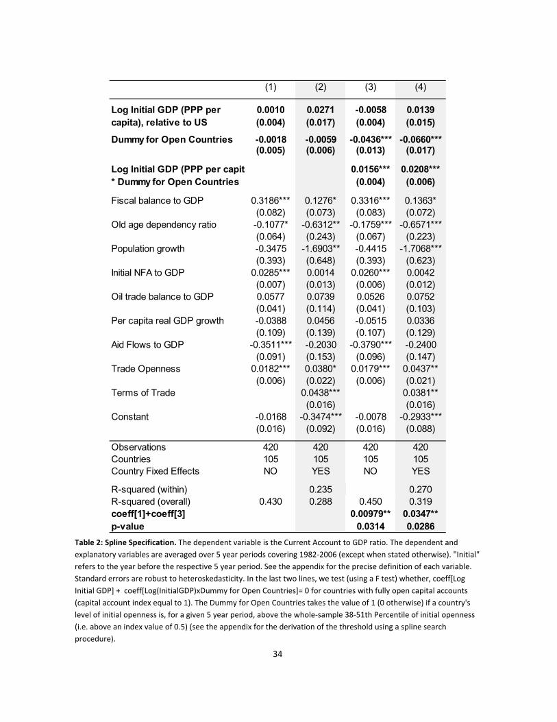
34
Table 2: Spline Specification. The dependent variable is the Current Account to GDP ratio. The dependent and
explanatory variables are averaged over 5 year periods covering 1982-2006 (except when stated otherwise). "Initial"
refers to the year before the respective 5 year period. See the appendix for the precise definition of each variable.
Standard errors are robust to heteroskedasticity. In the last two lines, we test (using a F test) whether, coeff[Log
Initial GDP] + coeff[Log(InitialGDP)xDummy for Open Countries]= 0 for countries with fully open capital accounts
(capital account index equal to 1). The Dummy for Open Countries takes the value of 1 (0 otherwise) if a country's
level of initial openness is, for a given 5 year period, above the whole-sample 38-51th Percentile of initial openness
(i.e. above an index value of 0.5) (see the appendix for the derivation of the threshold using a spline search
procedure).
(1) (2) (3) (4)
0.0010 0.0271 -0.0058 0.0139(0.004) (0.017) (0.004) (0.015)
Dummy for Open Countries -0.0018 -0.0059 -0.0436*** -0.0660***(0.005) (0.006) (0.013) (0.017)
Log Initial GDP (PPP per capita 0.0156*** 0.0208**** Dummy for Open Countries (0.004) (0.006)
Fiscal balance to GDP 0.3186*** 0.1276* 0.3316*** 0.1363*(0.082) (0.073) (0.083) (0.072)
Old age dependency ratio -0.1077* -0.6312** -0.1759*** -0.6571***(0.064) (0.243) (0.067) (0.223)
Population growth -0.3475 -1.6903** -0.4415 -1.7068***(0.393) (0.648) (0.393) (0.623)
Initial NFA to GDP 0.0285*** 0.0014 0.0260*** 0.0042(0.007) (0.013) (0.006) (0.012)
Oil trade balance to GDP 0.0577 0.0739 0.0526 0.0752(0.041) (0.114) (0.041) (0.103)
Per capita real GDP growth -0.0388 0.0456 -0.0515 0.0336(0.109) (0.139) (0.107) (0.129)
Aid Flows to GDP -0.3511*** -0.2030 -0.3790*** -0.2400(0.091) (0.153) (0.096) (0.147)
Trade Openness 0.0182*** 0.0380* 0.0179*** 0.0437**(0.006) (0.022) (0.006) (0.021)
Terms of Trade 0.0438*** 0.0381**(0.016) (0.016)
Constant -0.0168 -0.3474*** -0.0078 -0.2933***(0.016) (0.092) (0.016) (0.088)
Observations 420 420 420 420Countries 105 105 105 105Country Fixed Effects NO YES NO YES
R-squared (within) 0.235 0.270R-squared (overall) 0.430 0.288 0.450 0.319coeff[1]+coeff[3] 0.00979** 0.0347**p-value 0.0314 0.0286
Log Initial GDP (PPP per capita), relative to US
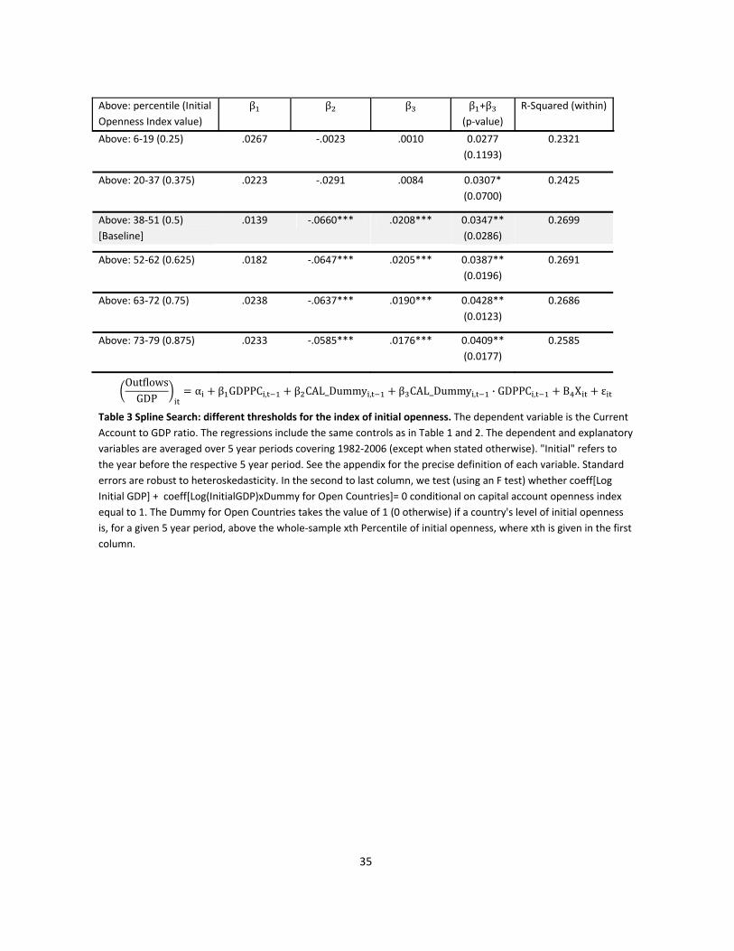
35
Above: percentile (Initial
Openness Index value)
β β β β +β(p-value)
R-Squared (within)
Above: 6-19 (0.25) .0267 -.0023 .0010 0.0277
(0.1193)
0.2321
Above: 20-37 (0.375) .0223 -.0291 .0084 0.0307*
(0.0700)
0.2425
Above: 38-51 (0.5)
[Baseline]
.0139 -.0660*** .0208*** 0.0347**
(0.0286)
0.2699
Above: 52-62 (0.625) .0182 -.0647*** .0205*** 0.0387**
(0.0196)
0.2691
Above: 63-72 (0.75) .0238 -.0637*** .0190*** 0.0428**
(0.0123)
0.2686
Above: 73-79 (0.875) .0233 -.0585*** .0176*** 0.0409**
(0.0177)
0.2585
OutflowsGDP
α β GDPPC , β CAL_Dummy , β CAL_Dummy , · GDPPC , Β X ε
Table 3 Spline Search: different thresholds for the index of initial openness. The dependent variable is the Current
Account to GDP ratio. The regressions include the same controls as in Table 1 and 2. The dependent and explanatory
variables are averaged over 5 year periods covering 1982-2006 (except when stated otherwise). "Initial" refers to
the year before the respective 5 year period. See the appendix for the precise definition of each variable. Standard
errors are robust to heteroskedasticity. In the second to last column, we test (using an F test) whether coeff[Log
Initial GDP] + coeff[Log(InitialGDP)xDummy for Open Countries]= 0 conditional on capital account openness index
equal to 1. The Dummy for Open Countries takes the value of 1 (0 otherwise) if a country's level of initial openness
is, for a given 5 year period, above the whole-sample xth Percentile of initial openness, where xth is given in the first
column.

36
Table 4.1: Robustness: Adding Control Variables. The dependent variable is the Current Account to GDP ratio. The
dependent and explanatory variables are averaged over 5 year periods covering 1982-2006 (except when stated
otherwise). "Initial" refers to the year before the respective 5 year period. See the appendix for the precise
definition of each variable. Standard errors are robust to heteroskedasticity. In the last lines, we perform two F
tests. First, whether coeff[Log Initial GDP] + coeff[Log(InitialGDP)xCapital Account Openness]= 0 for countries with
fully open capital accounts (capital account index equal to 1). Second, whether coeff[Reserve Accumulation] +
coeff[Reserve AccumulationxCapital Account Openness]= 0 for countries with fully open capital accounts.
(1) (2) (3) (4) (5) (6) (7) (8) (9) (10) (11) (12)
0.0096 0.0188 0.0094 0.0127 0.0082 0.0201 0.0092 0.0119 0.0571 0.0076 0.0076 0.0227(0.015) (0.019) (0.018) (0.014) (0.015) (0.017) (0.015) (0.018) (0.036) (0.017) (0.017) (0.021)
Index of Initial Capital Acc. Openness -0.0971*** -0.1131*** -0.1094*** -0.0913*** -0.0971*** -0.1457*** -0.0729** -0.0751** -0.0973*** -0.0984*** -0.0917*** -0.0775**(0.027) (0.029) (0.027) (0.029) (0.031) (0.023) (0.030) (0.031) (0.028) (0.031) (0.031) (0.029)
Log Initial GDP (PPP per capita) 0.0321*** 0.0413*** 0.0369*** 0.0310*** 0.0324*** 0.0431*** 0.0295*** 0.0304*** 0.0331*** 0.0338*** 0.0328*** 0.0348**** Index of Initial Capital Acc. Opennes (0.010) (0.010) (0.009) (0.010) (0.011) (0.009) (0.010) (0.010) (0.010) (0.011) (0.011) (0.009)
Fiscal balance to GDP 0.1238* 0.1520** 0.1548** 0.1657** 0.1346* 0.0190 0.1444** 0.1464** 0.1239* 0.0947 0.0962 0.1418**(0.070) (0.070) (0.062) (0.063) (0.069) (0.075) (0.068) (0.067) (0.071) (0.069) (0.069) (0.064)
Old age dependency ratio -0.6448*** -0.6703*** -0.6127*** -0.6016*** -0.6929*** -0.1860 -0.7250*** -0.7232*** -0.7057*** -0.6434*** -0.6342*** -0.6651***(0.226) (0.219) (0.211) (0.226) (0.223) (0.193) (0.216) (0.216) (0.213) (0.218) (0.221) (0.210)
Population growth -1.8911*** -2.2253*** -2.1654*** -2.5168*** -1.8636*** -0.6771 -1.7348** -1.7358** -1.7630*** -1.6724** -1.6554** -1.7823***(0.667) (0.567) (0.546) (0.517) (0.661) (0.722) (0.692) (0.689) (0.648) (0.651) (0.658) (0.625)
Initial NFA to GDP -0.0011 0.0064 0.0118 -0.0010 0.0013 -0.0037 0.0060 0.0063 0.0012 0.0011 0.0016 0.0131(0.012) (0.011) (0.010) (0.009) (0.012) (0.015) (0.012) (0.012) (0.012) (0.013) (0.013) (0.011)
Oil trade balance to GDP 0.0649 0.1071 0.1963 0.0877 0.0552 0.1370 0.0522 0.0500 0.0625 0.0495 0.0437 0.1404(0.108) (0.130) (0.120) (0.098) (0.107) (0.098) (0.096) (0.096) (0.105) (0.102) (0.104) (0.125)
Per capita real GDP growth 0.0421 0.0160 0.0997 0.0227 0.0672 0.0505 0.1418 0.1418 0.0355 -0.0180 -0.0134 0.0878(0.128) (0.144) (0.150) (0.131) (0.126) (0.122) (0.140) (0.140) (0.130) (0.116) (0.117) (0.161)
Aid Flows to GDP -0.1982** -0.2384** -0.2519** -0.2325 -0.3653** -0.4313** -0.4308** -0.2167 -0.2697* -0.2749* -0.4060***(0.094) (0.101) (0.107) (0.154) (0.141) (0.177) (0.175) (0.151) (0.156) (0.156) (0.123)
Trade Openness 0.0374* 0.0387 0.0289 0.0274 0.0352 0.0249 0.0512** 0.0511** 0.0374* 0.0314 0.0304 0.0415*(0.022) (0.023) (0.022) (0.021) (0.022) (0.020) (0.020) (0.020) (0.021) (0.022) (0.022) (0.021)
Terms of Trade 0.0369** 0.0398** 0.0347** 0.0395** 0.0402** -0.0143 0.0293* 0.0300* 0.0355** 0.0351** 0.0346** 0.0284*(0.017) (0.016) (0.016) (0.017) (0.017) (0.020) (0.016) (0.015) (0.016) (0.017) (0.017) (0.017)
Concessional loans to GDP -0.6638***(0.226)
Net grants to GDP -0.0459(0.233)
Private Credit to GDP ratio -0.0347*** -0.0221*(0.012) (0.012)
Growth in Private Credit to GDP -0.0982*** -0.0787***(0.023) (0.023)
Exchange Rate Regime 0.0030(0.003)
Banking Crisis 0.0072(0.007)
Years of Schooling 0.0071(0.007)
Institutions (ICRG) -0.1375*** -0.1237* -0.0983***(0.031) (0.068) (0.034)
Log Initial GDP*Institutions -0.0054(0.025)
Log Initial GDP Squared -0.0101(0.009)
Reserve Accummulation to GDP 0.3967*** 0.5950** 0.6656**(0.138) (0.236) (0.280)
Reserve Accummulation to GDP -0.4038 -0.5551* Index of Initial Capital Acc. Openness (0.456) (0.462)
Constant -0.2703*** -0.2987*** -0.2440*** -0.2854*** -0.2856*** -0.0709 -0.1655** -0.1744** -0.3098*** -0.2585** -0.2561** -0.2099**(0.094) (0.092) (0.086) (0.090) (0.094) (0.118) (0.081) (0.079) (0.091) (0.100) (0.101) (0.098)
Observations 407 383 381 390 420 286 394 394 420 418 418 359Countries 94 97 97 100 105 83 98 98 105 105 105 91Country Fixed Effects YES YES YES YES YES YES YES YES YES YES YES YESR-squared (within) 0.274 0.300 0.334 0.290 0.267 0.257 0.313 0.313 0.272 0.289 0.290 0.396R-squared (overall) 0.351 0.331 0.402 0.337 0.328 0.300 0.299 0.296 0.245 0.357 0.361 0.391coeff[1]+coeff[3] 0.0417** 0.0601*** 0.0463** 0.0437*** 0.0406** 0.0632*** 0.0387** 0.0423** 0.0902** 0.0414** 0.0404** 0.0575**p-value 0.0126 0.00337 0.0163 0.00591 0.0147 0.000196 0.0308 0.0471 0.0166 0.0179 0.0233 0.0109coeff[23]+coeff[24] (Reserves) 0.191 0.110p-value 0.516 0.670
Log Initial GDP (PPP per capita), relative to US
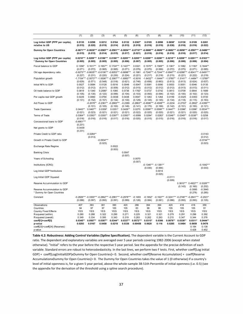
37
Table 4.2: Robustness: Adding Control Variables (Spline Specification). The dependent variable is the Current Account to GDP
ratio. The dependent and explanatory variables are averaged over 5 year periods covering 1982-2006 (except when stated
otherwise). "Initial" refers to the year before the respective 5 year period. See the appendix for the precise definition of each
variable. Standard errors are robust to heteroskedasticity. In the last lines, we perform two F tests. First, whether coeff[Log Initial
GDP] + coeff[Log(InitialGDP)xDummy for Open Countries]= 0. Second, whether coeff[Reserve Accumulation] + coeff[Reserve
AccumulationxDummy for Open Countries]= 0. The Dummy for Open Countries takes the value of 1 (0 otherwise) if a country's
level of initial openness is, for a given 5 year period, above the whole-sample 38-51th Percentile of initial openness (i.e. 0.5) (see
the appendix for the derivation of the threshold using a spline search procedure).
(1) (2) (3) (4) (5) (6) (7) (8) (9) (10) (11) (12)
0.0135 0.0298 0.0212 0.0164 0.0132 0.0367* 0.0105 0.0098 0.0658* 0.0130 0.0109 0.0261(0.015) (0.020) (0.019) (0.014) (0.015) (0.019) (0.016) (0.019) (0.038) (0.016) (0.016) (0.022)
Dummy for Open Countries -0.0671*** -0.0639*** -0.0585*** -0.0581*** -0.0654*** -0.0710*** -0.0608*** -0.0606*** -0.0682*** -0.0658*** -0.0597*** -0.0480***(0.015) (0.015) (0.014) (0.015) (0.017) (0.021) (0.016) (0.016) (0.016) (0.016) (0.017) (0.014)
Log Initial GDP (PPP per capita) 0.0210*** 0.0209*** 0.0186*** 0.0180*** 0.0205*** 0.0205*** 0.0209*** 0.0208*** 0.0218*** 0.0208*** 0.0201*** 0.0183**** Dummy for Open Countries (0.005) (0.005) (0.005) (0.005) (0.006) (0.007) (0.005) (0.005) (0.006) (0.006) (0.006) (0.004)
Fiscal balance to GDP 0.1356* 0.1617** 0.1657** 0.1724*** 0.1427** 0.0321 0.1575** 0.1569** 0.1361* 0.1082 0.1183* 0.1644**(0.071) (0.072) (0.065) (0.065) (0.071) (0.076) (0.070) (0.069) (0.072) (0.070) (0.071) (0.065)
Old age dependency ratio -0.6273*** -0.6635*** -0.6106*** -0.6053*** -0.6698*** -0.1981 -0.7240*** -0.7244*** -0.6947*** -0.6288*** -0.6041*** -0.6491***(0.227) (0.231) (0.220) (0.230) (0.224) (0.221) (0.217) (0.218) (0.215) (0.221) (0.222) (0.219)
Population growth -1.7154*** -2.0073*** -1.9306*** -2.3067*** -1.6950*** -0.5016 -1.6432** -1.6444** -1.5760** -1.5141** -1.4484** -1.5769**(0.629) (0.571) (0.548) (0.518) (0.621) (0.746) (0.656) (0.663) (0.613) (0.613) (0.624) (0.637)
Initial NFA to GDP 0.0027 0.0084 0.0128 0.0016 0.0048 -0.0047 0.0091 0.0090 0.0053 0.0051 0.0046 0.0135(0.012) (0.012) (0.011) (0.009) (0.012) (0.015) (0.012) (0.012) (0.012) (0.013) (0.013) (0.011)
Oil trade balance to GDP 0.0819 0.1340 0.2085* 0.1085 0.0736 0.1782* 0.0737 0.0742 0.0813 0.0709 0.0644 0.1689(0.105) (0.130) (0.122) (0.099) (0.104) (0.103) (0.093) (0.094) (0.102) (0.100) (0.102) (0.123)
Per capita real GDP growth 0.0229 0.0060 0.0794 -0.0038 0.0438 0.0547 0.1263 0.1264 0.0159 -0.0325 -0.0353 0.0720(0.131) (0.152) (0.157) (0.134) (0.130) (0.129) (0.145) (0.145) (0.134) (0.118) (0.115) (0.163)
Aid Flows to GDP -0.2078** -0.2361** -0.2683*** -0.2389 -0.2863** -0.4506*** -0.4508*** -0.2234 -0.2753* -0.2802* -0.4395***(0.101) (0.105) (0.100) (0.148) (0.141) (0.170) (0.169) (0.142) (0.151) (0.150) (0.121)
Trade Openness 0.0443** 0.0467** 0.0359* 0.0351* 0.0426** 0.0270 0.0599*** 0.0599*** 0.0447** 0.0396* 0.0396* 0.0534***(0.021) (0.023) (0.021) (0.021) (0.021) (0.022) (0.020) (0.020) (0.021) (0.021) (0.020) (0.020)
Terms of Trade 0.0364** 0.0393** 0.0355** 0.0397** 0.0393** -0.0099 0.0284* 0.0283* 0.0346** 0.0349** 0.0338** 0.0258(0.016) (0.016) (0.016) (0.017) (0.016) (0.020) (0.015) (0.015) (0.016) (0.016) (0.016) (0.017)
Concessional loans to GDP -0.6901***(0.231)
Net grants to GDP -0.0439(0.231)
Private Credit to GDP ratio -0.0284** -0.0143(0.013) (0.012)
Growth in Private Credit to GDP -0.0934*** -0.0744***(0.023) (0.023)
Exchange Rate Regime 0.0022(0.003)
Banking Crisis 0.0047(0.007)
Years of Schooling 0.0070(0.007)
Institutions (ICRG) -0.1346*** -0.1381** -0.1042***(0.030) (0.064) (0.033)
Log Initial GDP*Institutions 0.0014(0.025)
Log Initial GDP Squared -0.0111(0.009)
Reserve Accummulation to GDP 0.3810*** 0.4922*** 0.5328***(0.143) (0.160) (0.202)
Reserve Accummulation to GDP -0.3085 -0.3945* Dummy for Open Countries (0.278) (0.285)
Constant -0.2826*** -0.3300*** -0.2862*** -0.2981*** -0.2978*** -0.1493 -0.1652* -0.1627** -0.3241*** -0.2746*** -0.2641*** -0.2021*(0.088) (0.097) (0.093) (0.091) (0.089) (0.126) (0.084) (0.081) (0.086) (0.093) (0.093) (0.105)
Observations 407 383 381 390 420 286 394 394 420 418 418 359Countries 94 97 97 100 105 83 98 98 105 105 105 91Country Fixed Effects YES YES YES YES YES YES YES YES YES YES YES YESR-squared (within) 0.280 0.288 0.322 0.290 0.271 0.225 0.321 0.321 0.279 0.291 0.296 0.392R-squared (overall) 0.349 0.334 0.395 0.343 0.319 0.283 0.262 0.263 0.215 0.347 0.344 0.376coeff[1]+coeff[3] 0.0345** 0.0507** 0.0397** 0.0344** 0.0337** 0.0572*** 0.0315* 0.0306 0.0876** 0.0338** 0.0311* 0.0444**p-value 0.0293 0.0167 0.0458 0.0218 0.0336 0.00458 0.0620 0.116 0.0285 0.0484 0.0659 0.0476coeff[23]+coeff[24] (Reserves) 0.184 0.138p-value 0.428 0.452
Log Initial GDP (PPP per capita), relative to US

38
Table 5.1: Additional Robustness Tests. In column (1) the dependent variable is the sum of Current Account to GDP and the concessional loans to GDP ratio. In column (2) we
subtract Reserve Accumulation to GDP from the Current Account to GDP ratio. In column (3), the dependent variable is given by netting out reserve accumulation, net official
portfolio investment and net official other investment flows from the current account while in column (4) the dependent variable is the remainder. In column (5) we exclude
transition economies. In column (6) we include time fixed effects. In column (7) we use the Chinn and Ito index instead of the Quinn index as a proxy for capital account openness.
In the last two lines, we perform the F test of whether coeff[Log Initial GDP] + coeff[Log(InitialGDP)xCapital Account Openness]= 0 for countries with fully open capital accounts
(capital account index equal to 1).
(1) (2) (3) (4) (5) (6) (7)Excluding
concessional loansSubtracting Reserves
Excl. Transition Econ. Time FE Chinn & Ito
0.0098 -0.0058 0.0303 -0.0158 0.0108 0.0133 0.0262*(0.015) (0.017) (0.021) (0.016) (0.016) (0.016) (0.016)
Index of Initial Capital Account Openness -0.0974*** -0.0973*** -0.0799*** -0.0291 -0.0950*** -0.0948*** -0.0571**(0.026) (0.031) (0.030) (0.022) (0.031) (0.031) (0.028)
Log Initial GDP (PPP per capita) 0.0321*** 0.0346*** 0.0256** 0.0110 0.0315*** 0.0285** 0.0177*** Index of Initial Capital Account Openness (0.010) (0.011) (0.010) (0.008) (0.011) (0.012) (0.009)
Fiscal balance (to GDP) 0.1224* 0.0784 -0.1424 0.2961*** 0.1256* 0.1532** 0.1280*(0.070) (0.068) (0.087) (0.074) (0.071) (0.072) (0.067)
Old age dependency ratio -0.6255*** -0.5174** -0.2857 -0.3449* -0.6613*** -0.5582** -0.6249***(0.221) (0.210) (0.223) (0.191) (0.224) (0.218) (0.230)
Population growth -1.9017*** -1.0948* -1.2559** -1.9081** -1.8907*** -1.6016** -2.2717***(0.676) (0.611) (0.533) (0.760) (0.690) (0.701) (0.530)
Initial NFA (to GDP) -0.0021 -0.0010 0.0004 0.0140 0.0006 0.0009 0.0052(0.013) (0.013) (0.012) (0.013) (0.013) (0.012) (0.011)
Oil trade balance (to GDP) 0.0672 0.0234 -0.0078 0.0500 0.0752 0.0498 0.0428(0.108) (0.105) (0.113) (0.082) (0.138) (0.103) (0.109)
Per capita real GDP growth 0.0403 -0.1846* -0.1183 0.2057** 0.0566 0.0097 0.0743(0.128) (0.103) (0.138) (0.098) (0.138) (0.121) (0.133)
Aid Flows (to GDP) 0.0702 -0.2932* -0.1197 0.1948 -0.2371 -0.2015 -0.1148(0.164) (0.158) (0.154) (0.202) (0.154) (0.149) (0.128)
Trade Openness 0.0377* 0.0354* 0.0111 0.0123 0.0379* 0.0275 0.0260(0.022) (0.020) (0.027) (0.018) (0.022) (0.021) (0.020)
Terms of Trade 0.0361** 0.0272 0.0384* 0.0234 0.0383** 0.0389** 0.0460***(0.017) (0.017) (0.022) (0.021) (0.017) (0.017) (0.015)
Constant -0.2662*** -0.1882* -0.2987** -0.0842 -0.2802*** -0.2654*** -0.3475***(0.095) (0.101) (0.120) (0.095) (0.097) (0.094) (0.091)
Observations 407 417 412 413 397 420 413Countries 94 105 104 104 89 105 105Country Fixed Effects YES YES YES YES YES YES YESR-squared (within) 0.238 0.191 0.122 0.262 0.262 0.294 0.258R-squared (overall) 0.189 0.240 0.0795 0.0382 0.365 0.345 0.302coeff[1]+coeff[3] 0.0419** 0.0289* 0.0558** -0.00475 0.0423** 0.0418** 0.0439**p-value 0.0125 0.0941 0.0121 0.796 0.0178 0.0165 0.0185
Splitting private and public flowsPrivate Flows Public Flows
Log Initial GDP (PPP per capita), relative to US

39
Table 5.2: Additional Robustness Tests (Spline Specification). See table 5.1 for a description of the dependent variables. The Dummy for Open Countries takes the value of 1 (0
otherwise) if a country's level of initial openness is, for a given 5 year period, above the whole-sample 38-51th Percentile of initial openness (i.e. 0.5) (see the appendix for the
derivation of the threshold using a spline search procedure); in columns (7), we use the 72th percentile as a threshold based on the spline search procedure for the specification
including the Chinn and Ito index. In the last two lines, we test (using a F test) whether: coeff[Log Initial GDP] + coeff[Log(InitialGDP)xDummy for Open Countries]= 0 for countries
with fully open capital accounts (capital account index equal to 1).
(1) (2) (3) (4) (5) (6) (7)
Excluding concessional loans
Subtracting Reserves
Excl. Transition Econ. Time FE Chinn & Ito
0.0136 0.0006 0.0332 -0.0104 0.0144 0.0161 0.0295*(0.015) (0.017) (0.022) (0.017) (0.016) (0.015) (0.016)
Dummy for Open Countries -0.0677*** -0.0624*** -0.0581*** -0.0009 -0.0662*** -0.0653*** -0.0363(0.015) (0.017) (0.018) (0.018) (0.017) (0.016) (0.024)
Log Initial GDP (PPP per capita) 0.0212*** 0.0201*** 0.0170*** 0.0016 0.0208*** 0.0197*** 0.0124** Dummy for Open Countries (0.005) (0.006) (0.006) (0.005) (0.006) (0.006) (0.006)
Fiscal balance (to GDP) 0.1344* 0.0902 -0.1345 0.2990*** 0.1378* 0.1640** 0.1200*(0.071) (0.069) (0.087) (0.075) (0.072) (0.073) (0.068)
Old age dependency ratio -0.6093*** -0.5032** -0.2696 -0.3361* -0.6448*** -0.5474** -0.6150***(0.223) (0.215) (0.220) (0.191) (0.225) (0.217) (0.223)
Population growth -1.7260*** -0.9360 -1.1133** -1.8029** -1.7170*** -1.4300** -2.1905***(0.637) (0.582) (0.532) (0.738) (0.651) (0.663) (0.549)
Initial NFA (to GDP) 0.0019 0.0030 0.0039 0.0139 0.0046 0.0043 0.0042(0.012) (0.012) (0.012) (0.013) (0.012) (0.012) (0.011)
Oil trade balance (to GDP) 0.0841 0.0462 0.0079 0.0507 0.0920 0.0642 0.0449(0.105) (0.103) (0.114) (0.085) (0.134) (0.101) (0.109)
Per capita real GDP growth 0.0211 -0.1992* -0.1324 0.2019** 0.0376 -0.0118 0.0804(0.132) (0.106) (0.139) (0.097) (0.141) (0.123) (0.137)
Aid Flows (to GDP) 0.0634 -0.3010* -0.1412 0.2113 -0.2447 -0.2042 -0.0788(0.157) (0.154) (0.161) (0.206) (0.148) (0.147) (0.126)
Trade Openness 0.0445** 0.0434** 0.0194 0.0105 0.0447** 0.0332 0.0196(0.021) (0.019) (0.026) (0.018) (0.021) (0.021) (0.021)
Terms of Trade 0.0357** 0.0270* 0.0374* 0.0245 0.0377** 0.0387** 0.0459***(0.016) (0.016) (0.021) (0.021) (0.016) (0.016) (0.014)
Constant -0.2786*** -0.2055** -0.3061*** -0.1028 -0.2909*** -0.2795*** -0.3552***(0.089) (0.094) (0.116) (0.103) (0.093) (0.088) (0.085)
Observations 407 417 412 413 397 420 413Countries 94 105 104 104 89 105 105Country Fixed Effects YES YES YES YES YES YES YESR-squared (within) 0.245 0.189 0.129 0.260 0.269 0.300 0.259R-squared (overall) 0.195 0.191 0.0769 0.0340 0.368 0.351 0.291coeff[1]+coeff[3] 0.0348** 0.0207 0.0503** -0.00881 0.0352** 0.0358** 0.0419**p-value 0.0286 0.237 0.0240 0.608 0.0391 0.0274 0.0257
Splitting private and public flowsPrivate Flows Public Flows
Log Initial GDP (PPP per capita), relative to US

40
Appendix
A. Data
We mainly rely on the dataset assembled by Christiansen et al. (2009) and we update several
series. We employ data for 1980-2006 for all countries (110) with a population larger than one
million and for which data for our preferred index of financial openness (Quinn index) is
available (there are 5 countries for which not all the standard control variables are available).
As a preliminary screen on the data we exclude observations for which the dependent
variable and our baseline controls deviate by more than 4 standard deviations from their sample
mean in the fixed effects specification (i.e. using the country specific mean over time). This
makes sure that no extreme observation has an undue impact on the results.
Table A1 would indicate if a variable is constructed relative to trading partners: the weights
used are those employed by the Information Notice System (INS) system of the IMF to calculate
real effective exchange rates.
Variable Description
Balance of Payments Current Account/GDP The current account to GDP ratio is based on IFS spliced with data from
WEO. Reserve Accumulation/GDP
Reserve accumulation is measured by the negative of reserve flows taken from IFS (BOP statistics); if IFS data is missing, we use the change in the stock of reserves obtained from Lane and Milesi-Ferretti (2007).
Aid flows to GDP, net grants/GDP and concessional loans/GDP
Roodman (2006) computes a measure of foreign aid based on Official Development Assistance (ODA) data as total net aid minus debt forgiveness plus offsetting entries for debt relief. Concessional loans are constructed as foreign aid minus net grants. Net grants are constructed as total grants (also from ODA) minus debt forgiveness grants. The data are in millions of U.S. dollars and are computed relative to WEO nominal GDP.
Net official portfolio investment and official other investment
Official other investment (net) and official portfolio investment are taken from the IMF’s WEO database.
Financial Openness Index of Initial Capital Account Openness (Quinn)
Our preferred measure of financial openness is computed by Dennis Quinn (1997, updated to 2006) The index, which is normalized between 0 and 1 (1 for fully open countries), is based on the IMF’s Annual Report on Exchange Arrangements and Exchange Restrictions (AREAER).
Index of Initial Capital Account Openness (Chinn and Ito)
An alternative measure of capital account liberalization is taken from Chinn and Ito (2008); we use the data updated in July 2010. The index, which we normalize between 0 and 1, is also based on the IMF’s AREAER.
Income related variables Initial GDP (PPP per capita) relative to the US
Relative Income per capita is PPP income per capita relative to the U.S, both in constant 2005 international Dollars (rgdpl2). The index has a value

41
of 100 for the U.S. The data are from PWT 7.0. Real per capita GDP growth
The growth rate of GDP per capita (in PPP) is taken from PWT 7.0
Income Groups We aggregate countries into income groups based on the World Bank income group classification (as of 2006).
Demographics Old-age dependency ratio The old-age dependency ratio captures the share of people older than 64,
relative to the working age population, defined as the age group 15-64. The data are based on UN data, annualized by the World Bank.
Population growth The population growth data are computed from World Bank data, extended with UN projections.
External Net foreign assets/GDP Net foreign assets (NFA) are from Lane and Milesi-Ferretti (2007). If there
is no NFA data for a given country we use the cumulative current account. Oil trade balance/GDP The oil trade balance to GDP ratio is from WEO. Exchange Rate Regime As an indicator for the type of exchange rate regime we use the coarse
classification by Reinhart and Rogoff (2004a). We drop the observation if the index takes a value of 6 (dual market in which parallel market data is missing) and include observations with an index value of 5 (freely falling) into the 4 (freely floating) category. The higher the values of this index the more market determined (freer) the exchange rate.
Trade Terms of Trade The natural logarithm of terms of trade of goods and services. Data are
from WEO. Trade Openness The sum of imports and exports of goods and services divided by GDP (all
from WEO). Financial Development Private Credit/GDP Private Credit by Deposit Money Banks and Other Financial Institutions
relative to GDP is taken from the World Bank. Growth in Private Credit/GDP
Growth rate of Private Credit/GDP.
Years of Schooling Average years of schooling in the population aged 25 and over is taken from Barro and Lee (2000).
Fiscal: General Government Balance (GGB)/GDP
The general government balance relative to GDP, using the central government balance for countries where the general balance is not available. The data are from WEO.
Banking Crisis Our measure for banking crises is based on an updated version of the dummy variable constructed by Demirgüç-Kunt and Detragiache (1998). It takes a value of 1 for years in which a country experienced a banking crisis (0 otherwise).
Institutions (ICRG) To measure institutional quality we use a composite index measuring political risk compiled by the International Country Risk Guide (ICRG). The index is a weighted average of the following sub-components: Government Stability, Socioeconomic Conditions, Investment Profile, Internal Conflict, External Conflict, Corruption, Military Involvement in Politics, Religious Tensions, Law and Order, Ethnic tensions, Democratic Accountability, Quality of Bureaucracy.
42
B. Sample
110 Countries
Albania (ALB), Algeria (DZA), Argentina (ARG), Australia (AUS), Austria (AUT), Azerbaijan (AZE),
Bangladesh (BGD), Belarus (BLR), Belgium (BEL), Bolivia (BOL), Botswana (BWA), Brazil (BRA),
Bulgaria (BGR), Burkina Faso (BFA), Cambodia (KHM), Cameroon (CMR), Canada (CAN), Chile
(CHL), China (CHN), Colombia (COL), Congo (Rep.) (COG), Costa Rica (CRI), Cote d'Ivoire (CIV),
Czech Republic (CZE), Denmark (DNK), Dominican Republic (DOM), Ecuador (ECU), Egypt (EGY), El
Salvador (SLV), Estonia (EST), Ethiopia (ETH), Finland (FIN), France (FRA), Gabon (GAB), The
Gambia (GMB), Georgia (GEO), Germany (DEU), Ghana (GHA), Greece (GRC), Guatemala (GTM),
Haiti (HTI), Honduras (HND), Hong Kong (China) (HKG), Hungary (HUN), India (IND), Indonesia
(IDN), Iran (Islamic Rep.) (IRN), Ireland (IRL), Israel (ISR), Italy (ITA), Jamaica (JAM), Japan (JPN),
Jordan (JOR), Kazakhstan (KAZ), Kenya (KEN), Korea (Rep.) (KOR), Kyrgyz Republic (KGZ), Lao PDR
(LAO), Latvia (LVA), Libya (LBY), Lithuania (LTU), Madagascar (MDG), Malaysia (MYS), Mauritius
(MUS), Mexico (MEX), Morocco (MAR), Mozambique (MOZ), Nepal (NPL), Netherlands (NLD),
New Zealand (NZL), Nicaragua (NIC), Nigeria (NGA), Norway (NOR), Pakistan (PAK), Panama
(PAN), Paraguay (PRY), Peru (PER), Philippines (PHL), Poland (POL), Portugal (PRT), Romania
(ROM), Russian Federation (RUS), Rwanda (RWA), Saudi Arabia (SAU, Senegal (SEN), Sierra Leone
(SLE), Singapore (SGP), Slovak Republic (SVK), South Africa (ZAF), Spain (ESP), Sri Lanka (LKA),
Sudan (SDN), Sweden (SWE), Switzerland (CHE), Syrian Arab Republic (SYR), Tanzania (TZA),
Thailand (THA), Trinidad and Tobago (TTO), Tunisia (TUN), Turkey (TUR), Uganda (UGA), Ukraine
(UKR), United Kingdom (GBR), United States (USA), Uruguay (URY), Uzbekistan (UZB), Venezuela
(VEN), Vietnam (VNM), Zambia (ZMB), Zimbabwe (ZWE).
C. Spline Search
This section describes the spline search procedure employed to split countries in a
financially open and in a financially closed group. The spline search method aims at maximizing
the explanatory power of our baseline regression – i.e. the regression of the current account
balance relative to GDP on the standard controls X , CALP#, and an interaction term between
this dummy and (initial) income:
CAGDP
α β GDPPC β CALP# β CALP# · GDPPC α X ε
We set CALP# equal to 1 if a country’s level of openness is above the #th Percentile of
openness across all countries for a given panel window (and to 0 otherwise). We choose # such
that the within R2 of the regression is maximized. To obtain two groups that are large enough,
we restrict # to be between 20 and 80.

43
The method yields the 38-51th percentile for our baseline specifications – i.e. 5 year
averages with financial openness in initial terms – regardless of whether we include fixed effects
or not. The 38-51th percentile corresponds to an index value of financial openness of 0.5; as the
index of initial capital account openness is a step function, this corresponds to countries that are
above index values of 0.5. Figure 3 shows that this threshold splits observations in a closed and
an open group for which the effect of income on the current account balance differs markedly.

44
Appendix Tables
Table A1: Summary Statistics. # indicates deviation from trading partners. "Initial" refers to the year before the respective 5 year period.
Variable Mean Std. Dev. Min Max Observations
Current Account to GDP overall -0.0219 0.0532 -0.2689 0.1710 N = 467between 0.0495 -0.1874 0.0890 n = 110within 0.0306 -0.1323 0.1200 T = 4.24545overall 2.7491 1.2400 -0.4774 4.7607 N = 473between 1.2282 -0.2840 4.6877 n = 110within 0.1399 2.1890 3.2883 T = 4.3overall 0.5962 0.2828 0.0000 1.0000 N = 473between 0.2445 0.1250 1.0000 n = 110within 0.1554 0.0962 1.1462 T = 4.3
Fiscal balance to GDP # overall -0.0002 0.0380 -0.1749 0.1554 N = 449between 0.0284 -0.0638 0.1008 n = 107within 0.0250 -0.1112 0.0866 T = 4.19626
Old age dependency ratio # overall -0.0737 0.0580 -0.1763 0.0732 N = 453between 0.0573 -0.1615 0.0550 n = 107within 0.0106 -0.1121 -0.0246 T = 4.23364
Population growth # overall 0.0084 0.0101 -0.0174 0.0436 N = 453between 0.0100 -0.0163 0.0288 n = 107within 0.0036 -0.0081 0.0231 T = 4.23364
Initial NFA to GDP overall -0.3907 0.4938 -3.5789 1.3837 N = 459between 0.5115 -3.0497 0.9888 n = 110within 0.2243 -1.5437 0.5423 T = 4.17273
Oil trade balance to GDP overall 0.0071 0.0888 -0.1367 0.4335 N = 456between 0.0951 -0.1027 0.3883 n = 109within 0.0197 -0.1027 0.1248 T = 4.18349
Per capita real GDP growth overall 0.0215 0.0299 -0.0736 0.1608 N = 473between 0.0245 -0.0342 0.1175 n = 110within 0.0216 -0.0752 0.0921 T = 4.3
Aid Flows to GDP overall 0.0321 0.0515 -0.0012 0.3546 N = 455between 0.0502 -0.0001 0.2596 n = 110within 0.0200 -0.0551 0.1272 T = 4.13636
Trade Openness overall 0.6858 0.4439 0.1352 3.5362 N = 467between 0.4458 0.1911 3.4401 n = 110within 0.1278 0.1032 1.1943 T = 4.24545
Terms of Trade overall 4.6160 0.1974 3.4923 5.5199 N = 468between 0.1469 3.9042 5.0803 n = 109within 0.1447 4.0143 5.1718 T = 4.29358
Private Credit to GDP ratio overall 0.4575 0.3987 0.0187 1.8660 N = 420between 0.3770 0.0258 1.7574 n = 101within 0.1463 -0.1356 1.3620 T = 4.15842
Growth in Private Credit to GDP overall 0.0309 0.0879 -0.2825 0.4434 N = 416between 0.0549 -0.0570 0.2631 n = 101within 0.0762 -0.1946 0.3606 T = 4.11881
Exchange Rate Regime overall 2.2919 0.9356 1.0000 4.0000 N = 438between 0.8042 1.0000 4.0000 n = 106within 0.5043 0.2519 4.2919 T = 4.13208
Banking Crisis overall 0.1349 0.2771 0.0000 1.0000 N = 467between 0.1665 0.0000 0.7200 n = 110within 0.2209 -0.5851 0.8949 T = 4.24545
Years of Schooling overall 5.9893 2.8453 0.7420 12.2290 N = 317between 2.8583 0.9638 12.0190 n = 86within 0.5676 3.9068 7.7658 T = 3.68605
Institutions (ICRG) overall 0.6482 0.1511 0.2028 0.9542 N = 443between 0.1296 0.3099 0.9061 n = 102within 0.0704 0.4376 0.8422 T = 4.34314
Years of Schooling overall 5.9693 2.8428 0.7420 12.2290 N = 315between 2.8579 0.9638 12.0190 n = 86within 0.5694 3.8868 7.7458 T = 3.66279
Reserve Accummulation to GDP overall 0.0122 0.0210 -0.0836 0.1555 N = 469between 0.0153 -0.0047 0.1010 n = 110within 0.0145 -0.0727 0.1026 T = 4.26364
Log Initial GDP (PPP per capita), relative to US
Index of Initial Capital Account Openness
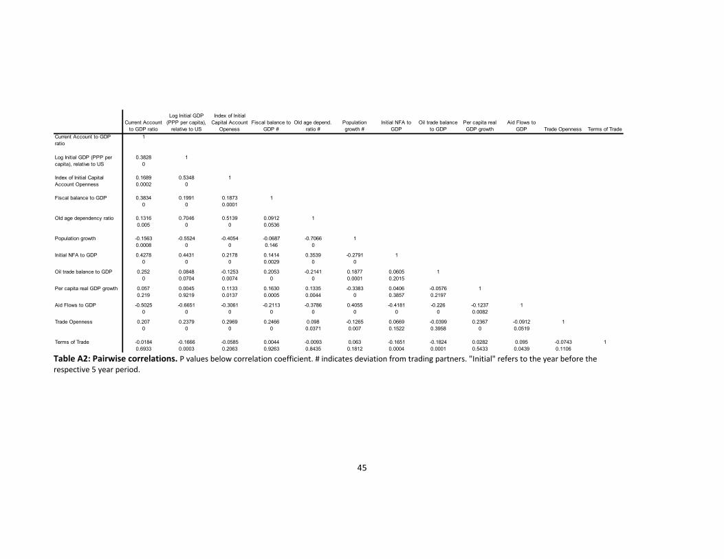
45
Table A2: Pairwise correlations. P values below correlation coefficient. # indicates deviation from trading partners. "Initial" refers to the year before the respective 5 year period.
Current Account to GDP ratio
Log Initial GDP (PPP per capita),
relative to US
Index of Initial Capital Account
OpenessFiscal balance to
GDP #Old age depend.
ratio #Population growth #
Initial NFA to GDP
Oil trade balance to GDP
Per capita real GDP growth
Aid Flows to GDP Trade Openness Terms of Trade
1
0.3828 10
0.1689 0.5348 10.0002 0
Fiscal balance to GDP 0.3834 0.1991 0.1873 10 0 0.0001
Old age dependency ratio 0.1316 0.7046 0.5139 0.0912 10.005 0 0 0.0536
Population growth -0.1563 -0.5524 -0.4054 -0.0687 -0.7066 10.0008 0 0 0.146 0
Initial NFA to GDP 0.4278 0.4431 0.2178 0.1414 0.3539 -0.2791 10 0 0 0.0029 0 0
Oil trade balance to GDP 0.252 0.0848 -0.1253 0.2053 -0.2141 0.1877 0.0605 10 0.0704 0.0074 0 0 0.0001 0.2015
Per capita real GDP growth 0.057 0.0045 0.1133 0.1630 0.1335 -0.3383 0.0406 -0.0576 10.219 0.9219 0.0137 0.0005 0.0044 0 0.3857 0.2197
Aid Flows to GDP -0.5025 -0.6651 -0.3061 -0.2113 -0.3786 0.4055 -0.4181 -0.226 -0.1237 10 0 0 0 0 0 0 0 0.0082
Trade Openness 0.207 0.2379 0.2969 0.2466 0.098 -0.1265 0.0669 -0.0399 0.2367 -0.0912 10 0 0 0 0.0371 0.007 0.1522 0.3958 0 0.0519
Terms of Trade -0.0184 -0.1666 -0.0585 0.0044 -0.0093 0.063 -0.1651 -0.1824 0.0282 0.095 -0.0743 10.6933 0.0003 0.2063 0.9263 0.8435 0.1812 0.0004 0.0001 0.5433 0.0439 0.1106
Current Account to GDP ratio
Index of Initial Capital Account Openness
Log Initial GDP (PPP per capita), relative to US

46
Table A3: Pairwise correlations of the demeaned variables. P values below correlation coefficient. # indicates deviation from trading partners. "Initial" refers to the year before the respective 5 year period. Variables are expressed in deviation from their time mean before calculating the correlation coefficient.
Current Account to GDP ratio
Log Initial GDP (PPP per capita),
relative to US
Index of Initial Capital Account
OpenessFiscal balance to
GDP #Old age depend.
ratio #Population growth #
Initial NFA to GDP
Oil trade balance to GDP
Per capita real GDP growth
Aid Flows to GDP Trade Openness
Terms oTrade
1
0.0328 10.4801
0.1168 -0.1340 10.0115 0.0035
Fiscal balance to GDP 0.1957 -0.1303 0.0941 10 0.0057 0.0464
Old age dependency ratio -0.2954 0.198 -0.2688 -0.1867 10 0 0 0.0001
Population growth -0.2379 0.2555 -0.247 -0.0755 0.3215 10 0 0 0.1103 0
Initial NFA to GDP -0.0275 0.2484 0.0223 -0.1621 0.1137 0.0323 10.5574 0 0.6332 0.0006 0.0164 0.4974
Oil trade balance to GDP 0.0742 0.002 0.0504 0.1444 0.0505 0.0278 -0.0549 10.1135 0.9666 0.283 0.0024 0.2879 0.5593 0.2466
Per capita real GDP growth 0.0948 -0.4655 0.2598 0.2666 -0.2144 -0.1333 -0.2225 0.0936 10.0406 0 0 0 0 0.0045 0 0.0457
Aid Flows to GDP -0.141 -0.0706 -0.1998 -0.0584 0.0865 -0.0383 -0.1023 -0.1607 -0.0532 10.0026 0.1326 0 0.2227 0.0696 0.4223 0.0305 0.0007 0.2577
Trade Openness 0.2118 -0.0081 0.347 0.1385 -0.404 -0.2256 -0.1553 -0.1535 0.2474 0.1328 10 0.8616 0 0.0033 0 0 0.0008 0.001 0 0.0045
Terms of Trade 0.1811 0.1272 -0.046 0.0845 0.1193 0.1297 0.0288 0.1964 0.0474 -0.1386 -0.0818 10.0001 0.0059 0.3205 0.0739 0.0112 0.0057 0.5406 0 0.3059 0.0032 0.0792
Current Account to GDP ratio
Log Initial GDP (PPP per capita), relative to US
Index of Initial Capital Account Openness