capital flows
DESCRIPTION
..TRANSCRIPT

1
The Reversibility of Different Types of Capital Flows to Emerging Markets*
Ozan Sula**
Western Washington University
Thomas D. Willett
Claremont Graduate University and
Claremont McKenna College
Abstract
We investigate whether some types of capital flows are more likely to reverse than others during currency crises. Earlier statistical testing has yielded conflicting results on this issue. We argue that the problem with the earlier studies is that the degree of variability of capital flows during normal or inflow periods may give little clue to their behavior during crises and it is the latter that is most important for policy. Using data for 35 emerging economies for 1990 through 2003, we confirm that direct investment is the most stable category, but find that contrary to much popular analysis, private loans on average are as reversible as portfolio flows.
JEL Classification: F32 Keywords: Capital flows; private loans; portfolio flows; foreign direct investment; currency crises.
* We thank Graham Bird, Eric Chiu, Arthur Denzau, Ozkan Eren, Hisham Foad, Sam Schreyer and Clas Whilborg and referees of this journal for their comments and suggestions. We are solely responsible for any errors. ** Send correspondence to Ozan Sula, Department of Economics, Western Washington University, Bellingham, WA 98225. Tel.: +1 360 6502530; fax: +1 360 6506315; email: [email protected].
2
1. Introduction
Currency crises that are accompanied by sharp reversals or “sudden stops” of
capital inflows have severe effects on emerging market economies including sizeable
output losses (Calvo 1998, Hutchison and Noy 2002, Edwards 2005).1
The standard approach to this hypothesis has generally been the evaluation of the
time series properties of different types of capital flows. Flows are labeled as “hot” or
The increased
frequency of these types of financial crises over the last decade and the fact that many of
these episodes were preceded by large capital inflows has generated heated discussions
about international capital flows (see e.g. Kim and Singal 2000). The standard
economist's presumption in favor of the efficiency of free capital flows has been seriously
challenged. A wide range of proposals have been made to control or more strictly
regulate capital flows, while other economists have argued that capital controls are
seldom effective and may generate more frequent rather than fewer crises. There is little
likelihood that such debate will be ended anytime soon, but progress is being made in
analyzing various relevant issues. This paper focuses on one such issue, that of whether
some types of capital flows are more stable than others i.e., are some types of capital are
more likely to reverse than others. Our approach complements the previous studies that
investigate the influence of the composition of capital inflows on an economy’s
vulnerability to a financial crisis (See e.g. Komulainen and Lukkarila 2003, Fernandez-
Arias and Hausmann 2001, Sula 2008).
1 The expressions ‘reversal’ and ‘sudden stop’ are used as interchangeably throughout the text. A reversal is
defined as a large fall in capital inflows, i.e., a change from a high inflow state to a low inflow or outflow
state.
3
“dangerous” based on their relative volatility. The underlying rationale is that a more
volatile form of capital will be more likely to fly out of the country in the event of a
crisis. Conventional wisdom says foreign direct investment (FDI) is the least volatile and
that short-term flows are generally more volatile than long-term ones. Portfolio flows
(stocks and bonds) are often singled out as being the most dangerous.
Empirical studies, however, do not always confirm these conventional views. For
example, Claessens et al. (1995) find that by their measure foreign direct investment is as
volatile as the other types of flows. The same study finds no significant difference
between long-term and short-term flows. In contrast, Chuhan et al. (1996), reach the
opposite conclusion. Sarno and Taylor (1997) find portfolio flows to be the most volatile
type of capital yet Willett et al. (2004) show that the largest outflows during the Asian
financial crises were bank loans. Gabriele et al. (2000) conclude that all types of capital
flow, including foreign direct investment, contributed to instability during the 1990s.
Levchenko and Mauro (2007) find that while the coefficient of variation for FDI flows to
emerging market countries was less than for other types of capital flows, its standard
deviation was higher than for debt and equity portfolio flows and for bank flows.
We argue that examining the volatility of capital flows during normal periods is
not necessarily informative about the behavior of capital flows during times of
unexpected crises.2
2 This is also a major theme of Levchencko and Mauro (2007) which was published after the initial version
of this paper had already been completed.
The contradictory findings in the empirical literature are due at least
in part to the limited time periods over which the volatility was investigated. Samples
were often dominated by periods of large inflows. From a policy perspective, the
4
magnitude of reversals during crises is more relevant than volatility during normal
periods. Mean-reverting monthly or quarterly volatility causes relatively minor problems
for balance of payments policy compared to a relatively stable inflow that displays a large
reversal during a crisis.
We investigate the link between volatility during normal periods and the size of
reversals during crisis periods. Our focus is on the behavior of total capital flows, foreign
direct investment, private loans and portfolio flows in 35 emerging market economies
between 1990 and 2003; a period dominated by the emerging market crises. We find that
volatility during inflow periods is not a good predictor of the size of reversals during
crises. Then, in a simple linear regression framework, reversals are regressed on the
accumulated previous capital inflows and the estimated model parameters are used to
compare the degree of reversibility of capital flows. Results from both types of tests
suggest that the composition of capital flows matters during crises. While FDI is found to
be the least reversible type of flow, loans are found on average to be as reversible as
portfolio flows.
Our results provide a link between the “sudden stop” literature, which investigates
the determinants and consequences of sudden stops, and the “hot money” literature,
which evaluates the volatility of different types of capital flows. The first literature has
not focused yet on the components of capital flow behavior while the latter has not
sufficiently differentiated between crises and normal periods.
The paper is organized as follows: Section 2 provides a background on different
types of capital flows and their expected behavior during crisis and normal periods.
Section 3 briefly summarizes the methodologies and findings of earlier studies. Section 4

5
examines the relationship between sizes of reversals during crises and volatility during
normal periods. Section 5 presents an alternative empirical framework for testing and
comparing the reversibility of different types of capital flows using linear regression
methods. Section 6 concludes.
2. Major Components of Capital Flows
In this section, we briefly review the major categories of private capital flows
investigated in this study and the arguments made about their likely relative volatility.
We categorize private capital flows based on the types of investor since changes in the
incentives facing different types of investors are the major determinants of the behavior
of flows during a crisis. This leads to three distinct types of capital flows for which data
is commonly available: foreign direct investments, portfolio flows and private loans.3
2.1. Foreign Direct Investment Flows
Foreign direct investment is widely considered to be the most stable form of
capital flows, both during normal and crisis periods. It consists mainly of fixed assets and
is highly illiquid and difficult to sell during crises. FDI is also influenced more by long-
term profitability expectations related to a country’s fundamentals than speculative forces
and interest rate differentials4
3 A common alternative is categorization based on maturity. In this case, private loans are divided into two
categories; short-term and long-term loans. In addition, portfolio debt flows are sometimes included in
these categories based on their maturity whereas portfolio equity flows become a separate category. We do
not use this alternative both because of insufficient data and concern that the standard methods of
distinguishing short from long-term flows are not able to capture this distinction well.
.
4 See Fernandez-Arias and Hausmann (2001) for a concise review of arguments on the stability of FDI.
6
The stability view of FDI has several caveats, however. One must distinguish
between the degree of reversibility of the bricks and mortar of investment as opposed to
the full range of activities associated with the investment. Once the physical investment is
made, it is irreversible, but the flow of funds associated with that investment is not
necessarily irreversible (Sarno and Taylor, 1997). While most of the fundamental factors
that determine FDI do not change suddenly during normal times, a sudden change in
perceptions of these fundamentals during a crisis may disrupt these flows of funds. Direct
investors may contribute to a crisis by accelerating profit remittances or reducing the
liabilities of affiliates toward their mother companies (World Bank, 2000). These are all
classified as non-FDI flows. This means that FDI may cause instability by allowing other
types of flows to mask it.5
Much of the observed stability of direct investment flows is likely to be real
however. The depreciation that often accompanies a crisis can increase the profitability of
many types of direct investments. For example, if the market value of a firm falls
substantially, then inflows may be generated to take advantage of a perceived bargain
(Krugman, 2000).
Flows may enter the country under the heading of FDI and
leave under other accounts. If financed locally FDI may also create outflows such as bank
lending or portfolio outflows. Foreign investors can use the physical assets as collateral to
obtain a loan from banks and can then place the funds abroad (Bird and Rajan, 2002). In
addition, the distinction between portfolio flows and FDI can be somewhat arbitrary
since, according to the International Monetary Fund’s (IMF) classification, an equity
investment above 10 percent is considered FDI.
5 See Sula (2008) for empirical evidence against this hypothesis.

7
2.2. Portfolio Flows
Portfolio flows consist of both bond and equity investments. Portfolio investors
can sell their stocks or bonds more easily and quickly than FDI and these flows are often
considered to be the hottest of the various major types of capital flows.
Portfolio flows are also more susceptible to informational problems and herding
behavior. For example, Calvo and Mendoza (2000) show how global diversification of
portfolios and informational problems can cause rational herding behavior in financial
markets.6
While these factors can explain high volatility of portfolio flows, they neglect an
important feature of stock and bond markets. Concerns about portfolio flows come
mainly from the high liquidity; at the first sign of trouble investors can easily sell their
stocks and bonds. However, most of the time portfolio investors are too late to sell their
assets without incurring large losses. To the extent that markets are efficient, the
immediate hit to asset prices means that future increases are roughly as likely as
decreases. With more price adjustment there is less incentive for future quantity
adjustments. The price of these assets can adjust very quickly (Bailey et al. 2000, Willett
et al 2004, Williamson 2001). Therefore, the high volatility of portfolio flows during
normal times does not necessarily imply a large reversal during crises. There is empirical
evidence that financial markets in emerging market economies do deviate from full
Furthermore, Haley (2001) argues that mutual fund managers are small in
number and they show similar patterns in their trading decisions. They tend to invest or
leave a market at the same time causing high instability.
6 Calvo and Mendoza’s model applies primarily to portfolio flows.

8
efficiency,7
2.3. Private Loan Flows
so we would not necessarily expect the full effect of a crisis to be on
portfolio prices, rather than quantities. For example, momentum trading or panic could
cause price declines to generate outflows. However this capacity for large rapid price
adjustments suggests that quantity adjustments may not always be large.
Private loans consist of all types of bank loans and other sector loans including
loans to finance trade, mortgages, financial leases, repurchase agreements, etc. They have
been a relatively neglected category.8 Sarno and Taylor (1997) suggest that they are the
least important fraction of capital flows in the 1990’s in terms of relative size. They argue
that, “Because of the liquidity of commercial loans to developing countries once they are
made, one might expect commercial banks to look more closely at the underlying
economic fundamentals before committing funds and therefore to be less prone to sudden
changes of heart. Moreover once funds are committed this way, it may seriously
jeopardize a bank’s chances of recovering its investment if lending is suddenly
withdrawn.” Gabriele et al. (2000) classify loan flows as somewhat volatile, in between
portfolio flows and FDI, but not very important compared to the other types of capital
flows. As will be illustrated in the following sections, recent data provides a strongly
contrasting picture on the importance of private loans during the 1990s. During the Asian
crises, private loans had the largest reversals.9
7 For a recent review of studies on this issue, see Williamson 2005.
8 See, however, Bailey et al. 2000, Willett et al. 2004, and Williamson 2001 and 2005.
9 Ibid.

9
Due to the illiquid nature of bank loans, their prices do not adjust automatically,
and thus banks adjust the quantity of lending instead. During times of financial distress,
uncertainty and risk rise which in turn is reflected in interest rates. Depending on the
severity of the situation, rising interest rates further increase the probability of a default,
making loan flows more risky. In this case, banks may have larger incentives to pull out
from crisis countries in order to cut their losses (Bailey et al. 2000, Willett et al. 2004,
Williamson 2001). Credit rationing takes place and foreign investors retrieve their short-
term debt and halt lending and rolling-over existing long-term debt. This implies that
volatility of loans may differ substantially during crisis and normal periods.
In summary, there are strong reasons to believe that FDI will be the most stable
type of private capital flow, although the true degree of stability is likely to be somewhat
less than is captured in official statistics. It is not clear, however, whether we should
expect substantial differences in the degree of instability of portfolio investment versus
loans. There are important counter arguments to the popular view that portfolio flows are
the most dangerous and it is difficult, if not impossible, to judge a priori the relative
importance of the arguments on each side. Thus we must turn to the empirical evidence.
3. Previous Empirical Research on Volatility Rankings
The majority of existing empirical studies focus on the overall volatility of capital
flows10
10 See Griffith-Jones (1998) for a comprehensive survey on composition of capital flows and volatility.
. The implicit assumption is that if time series data shows high volatility for a
particular type of flow, then this capital flow component is “hot” and has a high potential
for reversal in a crisis. These studies use various statistical methodologies ranging from
10
simple standard deviation calculations to more sophisticated econometric techniques such
as Kalman filtering and vector autoregression.
Claessens et al. (1995) analyze the distinction between short and long-term capital
flows during the 1970s and 1980s.11
In a later study, Chuhan, Gabriel and Popper (1997) reach the opposite conclusion
for the period between 1985 and 1994.
They compared various volatility measures like
standard deviations and coefficients of variation for flow types as well as persistence,
through looking at autocorrelations, half-life responses, and the predictability of flow
series using an autoregressive model. They find very little evidence for significant
distinctions among types of flows.
12
Sarno and Taylor (1999) apply Kalman filtering to measure the relative size and
statistical significance of the permanent and temporary components of various types of
capital flows for 1988 to 1997.
They argue that similar univariate patterns
among series can mask substantial differences if types of capital flows interdependent,
and conclude that composition matters.
13
11 The time period varies across countries. Overall they cover the period between 1972 and 1992. Their
long-term flows are bonds, longer maturity loans and reserves. Short-term flows are bank deposits, shorter
maturity loans and other short-term official flows.
They argue the flows that are more likely to have sudden
reversals would have large temporary, reversible components. They find that the
permanent component in explaining the variance of flows is very large in direct
investment, and that portfolio flows have a large temporary and reversible component,
12 They classified their capital flows into portfolio (equities and bonds), FDI and long-term and short-term
other investments.
13 They classified capital flows as bonds, equities, FDI, official flows and commercial bank credit.

11
suggesting that portfolio investment is particularly dangerous. However, their study
includes only a small portion of the Asian crisis in which bank flows show the largest
reversal.
IMF (1999) uses sign changes and coefficients of variation of net capital flows to
assess volatility during the 1980s and 1990s. They find that while FDI is the least volatile
flow, long-term flows have been as volatile as the short-term flows. Gabriele et al. (2000)
also employ coefficient of variation and standard deviation measures to assess the
volatility and instability of capital flow types for the period 1975 to 1998.14
An important problem of the previous studies is the limited time periods over
which capital flow volatility was studied. Most of these studies focus on time periods
dominated by net inflows and include little data on the recent major currency crises in
emerging economies. When volatility is analyzed for a longer period without a distinction
between crisis and non-crisis periods, the implicit assumption is that components of
capital flows behave similarly in both periods. As we discussed in the previous section,
investors may act on different incentives during crises than during normal times. To the
extent that the difference in behavior is large, the volatility approach will be misleading,
especially if crisis periods are under-represented in the sample.
They find that
volatility and instability increased during the 1990s. They also use Granger causality tests
to investigate the relation between the inflows and outflows of different types of flows.
They conclude that short-term flows are particularly volatile, but that all types of capital
flows contributed to the instability during the 1990s.
14 Their short-term flows include portfolio flows, short-term private loans, foreign currency and deposits
and official short-term flows.

12
In a more recent study Levchenko and Mauro (2007) analyze the behavior of
FDI, Portfolio flows and other flows (including bank loans) to a large panel of emerging
markets and developing nations during 1970-2003. Besides using the standard volatility
measures they, like our paper, investigate the size of reversals during sudden stop crisis,
and find FDI to be the most stable type of capital flows. Their results show that during
sudden stop crises portfolio equity flows have a limited role, portfolio debt flows reverse
but recover rather quickly and other types of flows experience significant drops without
an immediate recovery.
4. Volatility as a Measure of Reversibility: Extending the Previous Work
To assess reversibility of different types of capital flows, we reapply the volatility
approach with separation of crisis and non-crises periods. The sample contains 35
emerging market countries from 1990 to 2003.15
15 Countries are included if they are contained in the Emerging Markets Bond Index (EMBI+) or the
Morgan Stanley Country Index (MSCI) following Fischer (2001). In addition Bangladesh, Botswana,
Croatia, Hong Kong, Romania, Syria, Uruguay and Zimbabwe are added to the sample due to their large
capital inflows during the 1990s.
The time period starts with the return of
substantial debt flows after the debt crisis and the majority of countries in the sample
liberalized their capital accounts and ends around the time where reserve accumulations
become the new policy trend. The bulk of the surge of capital inflows and the subsequent
sudden stop crises in emerging markets are also witnessed during this period. Of course
the current global crisis will provide important additional evidence but sufficient data is
not yet available to include this episode in our analysis. Extending the data for the
13
additional few years after 2003 for which data is now available would lead to biased
results by including just the inflow period and not the following stop.
Capital flows are classified as foreign direct investment, portfolio investment
(including portfolio debt and equity flows), private loans (including both bank and other
sector loans), and total capital flows (which is the financial account of the balance of
payments including all private and official flows).16
In order to differentiate between crisis years and normal periods, we employ the
standard methodology in the literature, where currency crises are identified by large
changes in exchange market pressure indices
17. The indices are defined as a weighted
average of monthly real exchange rate changes and monthly (percentage) reserve losses.18
Table 1-a presents net capital flows as a percentage of GDP for each type of
capital during crisis years.
19
16 See Appendix A for data sources.
The table shows that except for private loans, all types of
capital continued to flow in to the emerging economies during the crisis years. Portfolio
flows decrease during crises, but net outflows occurred only from Indonesia, Malaysia
and Turkey.
17 We use a threshold of 2.5 standard deviations. Studies also often use either two or three standard
deviations. Our results are robust to alternative crises calculations. See Appendix B for the list of currency
crisis indentified by the methodology.
18 In the original formulation of crises index by Eichengreen et al. (1996) interest rates were also included
but because of data problems interest rates have typically been excluded from the construction of these
indices for developing countries. For further discussion of these issues see Willett et al.(2005) and the
references cited there.
19 We used GDP as a scale measure. Other possible alternatives are the money supply and international
reserves.

14
Capital flows do not always need to turn negative to cause problems. Where
previous capital inflows were large, a sizeable fall in inflows could cause a financing or
adjustment problem. Thus, for example, a fall in capital inflows from five to one percent
of GDP could cause more problem than a reversal from a 1 percent inflow to a 1 percent
outflow20
1
1
−
− −
t
tt
GDPKK
. A measure that would capture the magnitude of the fall in capital inflows is the
following:
(1)
where K is a capital flow component. A larger positive value for this ratio indicates a
larger reversal. 21
Table 1-b presents reversal measures. Except for FDI, all types of capital flows
display large reversals during crises. The fall in capital inflows is largest for private loans
during the Asian crises. Other emerging market crises witness similar falls in both
portfolio and loan flows. FDI usually does not reverse. During the Asian crises, the
largest outflows were from the private loan category, presumably mainly bank loans.
Thailand, for example, experienced a fall in capital inflows of 17 percent of GDP and
almost all of this fall was in private loans. Reversals in Indonesia and Philippines were
predominantly from portfolio investors. Both crises in Turkey were associated with
20 A good example is the case of the Mexican crisis in 1994. The data suggest that during the crisis,
portfolio inflows were positive and private loans were negative. On the other hand, the reversal measure
provides a more accurate indication, as the fall in portfolio flows to Mexico was about 5 percent of GDP
and the fall in the private loans was almost 10 times smaller than that.
21 Radelet and Sachs (1998), and Rodrik and Velasco (1999) use this measure to identify capital account
reversals.

15
reversals in private loans, while the reversals in Russia and Mexico were mainly portfolio
flows. There is no consistent pattern across different crises for the size of private loans
and portfolio flow reversals.
Next, volatility for each type of flow is calculated. Previous studies have
employed several different methodologies, the most popular ones being the standard
deviation and coefficient of variation. The standard deviation provides an absolute
measure of variability, but does not relate variability to the size of the economy. In
addition, it may be biased if capital flows are non-stationary.
The coefficient of variation, the ratio of standard deviation to its mean does relate
variability to size, but of the capital flows, not the size of the economy. By this measure
flows fluctuating between 1 and 2 percent of GDP during normal times would be deemed
more variable then those varying between 4 and 6 percent of GDP only when a crisis hits.
From a policy perspective, the size of absolute variation or variation in relation to
the average level is not likely to be as important as the variation in relation to the size of
the country’s international reserves, national income or financial sector. The standard
deviation of the reversal term (1) satisfies this requirement and handles the caveats of
standard deviation as an indicator of volatility: using GDP as a denominator enables
comparison of variability across countries and conveys policy relevant information about
the magnitude of flows. Furthermore, taking the difference of capital flows usually takes
care of potential non-stationarity problems.
Tables 2-a and 2-b present coefficient of variations and standard deviations of
each type of capital flow, calculated based on the reversal term (1). The upper panel in

16
each table shows the volatility calculated using the whole sample. The bottom panel
presents calculated volatility that excludes the crisis years.22
There is no clear pattern for coefficients of variation across countries and different
flows. The sizes of coefficients are very sensitive to the inclusion of crises years in the
sample. These simple statistics can be interpreted in two ways. One is that there is no
systematic difference in terms of volatility among different types of capital flows. The
other is that the coefficient of variation is not a reliable indicator of policy relevant
volatility. We are inclined towards the second explanation.
There are several consistent patterns in Table 2-b. FDI has the lowest volatility
among all flows and it does not differ substantially between volatility calculated from the
whole period and non-crisis periods. The volatility of private loans is usually close to or
higher than the volatility of portfolio flows. Volatilities calculated for the whole period
are higher than non-crisis period volatilities for total flows, and this usually also holds for
private loans. On the other hand, excluding crisis years does not decrease the volatility of
portfolio flows.
This evidence suggests that private loans are as volatile as portfolio flows and that
FDI is stable. The relevant question for policy is whether a higher measured volatility
implies a higher reversibility. Next, we present the correlations of reversal size during
crises and volatility calculated from the whole period and from non-crisis periods for
each type of flow.
Table 3-a shows that correlations are very low when the coefficient of variation is
used as the volatility indicator. The standard deviation, provides a closer association with
22 We exclude both the year of the crisis and the following year to isolate the normal-period volatility.
17
the sizes of reversals (Table 3-b). When crisis years are excluded from the standard
deviation calculations, the correlation coefficients are low for total flows and private
loans (0.26 and 0.21). Thus the volatility of private loans during normal times has little, if
any, explanatory power for their behavior during crisis periods. As would be expected,
the correlations increase dramatically when crisis years are included, but this is of little
help in forecasting vulnerability.
5. An Alternative Empirical Model of Reversibility
In discussions of sudden stops and the variability of capital flows it is often
assumed that international capital will act, at least to some degree, differently from
domestic capital. On this assumption a country is likely to have larger outflows in a
crisis, the greater is the amount of foreign capital already in the country, i.e., the larger
have been the previous capital inflows the larger the capital outflows in a crisis. What
portion of the existing capital flows out is an empirical question that can aid us to
measure a particular type of capital’s reversibility.
We therefore investigate the size of net outflows in relation to the preceding
cumulative capital. We know, of course, that domestic capital also tends to flow out
during crises. Indeed, many countries that have attracted little foreign capital have had
huge capital outflows from capital flight. Thus, it is unclear how strong a relationship we
should expect to find between outflows during crises and previous capital inflows.
Ideally, we would like to analyze separately reversals of both domestic and foreign flows.
18
Unfortunately, data that would allow us to conduct such analysis is not publicly available
on a broad basis.23
Consider the following equation for the size of reversals:
tijtijjjtij A ,,,,,, Reversal εβα ++= , (2)
TtNiJj
,...2,1,...2,1,...2,1
===
where j indexes the type of capital flow, i indexes countries and t indexes crisis
years. The dependent variable is the reversal measure for the capital flow type j in
country i during the crisis in year t. tijA ,, is the accumulated previous capital inflows; it is
constructed as the sum of the previous five years of capital flows relative to GDP.24
The expected sign for the slope coefficient is positive. Heterogeneity across types
of flows is introduced through the constant term, slope coefficients and error terms. If
components of capital flows differ in terms of their reversibility, then by comparing the
significance and size of the parameters of the model for different values of j, a
reversibility ranking could be established. We estimate the parameters utilizing four
model specifications that treat heterogeneity in alternative ways.
It is worth noting that equation (2) does not include any control variables. There
are two reasons for this. First, our emphasis is on correlation not causation. We want to 23 Domestic residents’ transactions are represented by the assets on the balance of payments statistics. Data
on these are limited for portfolio flows and private loans. Our net capital inflow measure includes assets for
some countries but it is not possible to assess the size of possible asset outflow during a crisis with the
available data.
24 Our analysis is not sensitive to the number of previous years of foreign capital accumulation. Results based on the sum of three and four years of capital flows relative to GDP are available on request.
19
obtain a reversibility ranking simply by comparing the association between accumulated
inflows and reversals of different types of capital. For example, if a nation has a large
current account deficit, one might expect a more severe currency crisis which will cause
more capital outflows. If we control for the deficit however, we can not capture its effect
on the existing capital, and this effect is what makes a particular type of capital more
reversible. A highly reversible type of capital will be more sensitive to the other factors in
the economy and hence more likely to flow out during crisis. Second, due to the small
number of observations, and high correlation among potential control variables, including
them lead to multicollinearity problems.
Nevertheless, as a robustness check we run a second regression for each model
including four control variables that are likely to affect the magnitude of capital reversals
during crisis: current account balance/GDP ratio, real exchange rate appreciation (a
positive value represents real exchange rate appreciation), type of the exchange rate
regime (1 for intermediate regimes, 0 otherwise) and degree of capital mobility (an index
between 0 and 100, 100 being the highest degree of capital mobility).25
5.1. Ordinary Least Squares Model for Total Net Capital Flows
In the first model, we measure the overall reversibility of capital flows. That is we
take the reversal of total capital flows as the dependent variable and regress it on its
cumulative flows. If different types of flows are similar in terms of their reversibility as
suggested by Claessens et al. (1995) and Gabriele et al. (2000), then we would expect to
find a significant positive coefficient for the total cumulative inflows. Alternatively, if
they have different reversal potential, then without taking the composition into
consideration, previous total net capital flows should not explain the size of total reversal 25 See Appendix A for data sources.

20
as it will be seriously biased. The first column of Table 4-a shows that the coefficient for
accumulated inflows and the overall fit of the model are insignificant; previous total
cumulated capital inflows have no explanatory power over the size of total reversals
during crises.26
5.2. Pooled Ordinary Least Squares Model with a Robust Covariance Structure
In Table 4-b, we add the control variables and the overall fit of the model
improves, but the coefficient on our key variable is both statistically and economically
insignificant.
Sometimes countries receive outside financial help from developed nations and
the IMF during crises. Since total capital flows are measured by the financial account of
the balance of payments, bailouts and emergency loans may be included, and this would
not reflect the correct size of a reversal. To test for differences of reversals across capital
flow types, we pool the observations for the three major types of capital flows. In this
model, the slope coefficient and the constant term are assumed to be the same for all
types of capital flows. Differences across types of capital flows may arise from different
variances or from the covariances of the disturbances of the equations. Once more, we
assume away different degrees of reversibility in this model and account for differences
in the error term.
The model is estimated with the feasible generalized least squares method. We
control for the groupwise heteroscedasticity where each group is a major type of capital
flow. Results are presented in the second column of Tables 4-a and 4-b. They are the
same as the first model’s. In regressions both with and without the controls, all
coefficients are insignificant and the overall fit of the model is low.
26 Several studies have found the size of total capital flows to be significant in explaining crises likelihood (See for example: Radelet and Sachs 1998, Domac and Peria 2000, Sula 2008). What makes our analysis different is the focus on the reversal size instead of the crisis probability.

21
5.3. Least Squares Dummy Variable Model
Results from the first two models show that we cannot explain the size of
reversals with accumulated inflows if we assume that all types of capital flows have the
same behavior during crises. We now investigate whether we find a relationship when the
composition of capital flows is taken into consideration.
Our previous analysis suggests that capital flow types have different degrees of
reversibility. The dummy variable approach takes jα to be a flow type specific constant
term in the regression model. The effects of the different natures of capital flows are
reflected in this constant term. Using the same pooled observations from the previous
model, we add two dummy variables, one for portfolio flows and one for FDI. The
dummy for private loans is excluded from the regression so the constant term becomes
the base for this type of flow. The dummy coefficients for the remaining capital flow
types measure the extent to which they differ from private loans. In this case a negative
sign for these dummies indicates less reversibility relative to private loans, and a positive
and significant constant term would reflect greater reversibility of private loans.
The third columns of Tables 4-a and 4-b present the results. The slope coefficient
is positive and significant in both regressions indicating that there is a positive
relationship as expected between accumulated inflows and reversals if one controls for
the type of capital flow.
The coefficient for the FDI dummy is negative and significant in both regressions.
If the cumulative inflows of both FDI and Private loans are the same, the size of FDI
reversal will be on average approximately 3 percentage points (percentage of preceding

22
year’s GDP) less than private loans. This finding confirms the stability of FDI as the
volatility measurements from the previous section indicated.
In the regression without the control variables, the constant term is positive and
significant, demonstrating a high reversibility of private loans. The dummy coefficient
for portfolio flows is close to zero and insignificant; portfolio loans are as reversible as
private loans. When the other variables are added to the regression, the constant term
becomes insignificant but our conclusion still holds.
5.4. Seemingly Unrelated Regressions Model
So far the slope coefficients have been restricted to be the same across flow types.
It is quite plausible that the slopes would differ across capital flow types. In this case, the
slope coefficient would also provide an indication of reversibility. For example, based on
our previous findings, one would expect a lower coefficient of accumulated inflows for
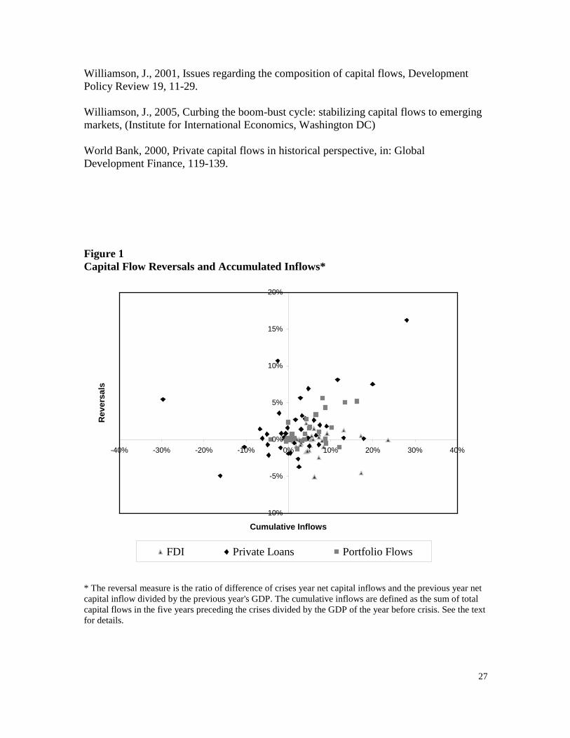
FDI. Figure 1 illustrates the relationship of cumulative flows and reversal sizes; it
provides some preliminary evidence in favor of this model.
One way to estimate the slopes is to run OLS regressions for each flow type, and
then compare coefficients. However, a more realistic approach is to assume that
disturbances for each flow type during a given crisis are correlated. During unexpected
crises, risk perceptions and expected returns for all types of capital flows can change
dramatically and it is safe to assume that these changes have some common terms. The
main question is whether the magnitude and direction of these changes are equal.
Otherwise would this affect the sizes of the reversals. By relaxing the constraint that all
three types of flows have the same slopes, we obtain a three-equation seemingly
unrelated regression model.
23
The results are shown in Tables 5-a and 5-b. The slope coefficient for private
loans is significant and larger than any other flow type. If one ranks the slope coefficients
as well as the constant terms, the same order is reached as in the previous model. In both
regressions the slope coefficient of private loans is greater than for the portfolio flows but
the difference is not statistically significant. Both of these coefficients are significantly
greater than the FDI coefficient. We find a negative and insignificant coefficient for FDI.
This also confirms that FDI does not tend to reverse during crises. The explanatory
powers of the models are also stronger compared to previous models. Except for the FDI
regression, both private loan and portfolio flow regressions have larger R-squares.
6. Conclusion
In this study, we investigate the reversibility of components of capital flows to
emerging markets. The paper’s central focus is on differentiating crisis from non-crisis
periods. Our empirical analysis confirms that foreign direct investment is the most stable
type of capital flow during crises. Contrary to the conventional wisdom, portfolio flows
are not clearly the most reversible; private loans are as reversible as portfolio flows on
average. We also find that volatility of capital flows in normal periods is not a good
predictor of the size of their reversal during crisis.
Of course the results of the empirical analysis do not provide a full explanation of
the size of reversals during crises. However, they do provide support for the hypothesis
that the composition of capital flows matters for sudden stops and the magnitude of
capital outflows during currency crises. We find that both private loans and portfolio
flows can be highly reversible, with the former being the most reversible in most of the
crisis episodes. We also confirm the conventional view of FDI. This type of flow is quite
stable and the least reversible. However a word of caution is needed. This paper does not
24
investigate the possibility that flows that enter a country under the disguise of FDI may
leave under the mask of other flows.
The evidence presented in this paper does not speak directly to the debate over
capital controls, but it does have important implications for the demand for international
reserves and international risk management. While substantial inflows of financial capital
generally do signal that a country has been doing many things right, they may also signal
that the potential for future currency and financial crises is increasing. Such potential
warning signs should be noted by both national governments and private investors.
This suggests that governments should set aside some of the reserve inflows
accompanying large financial capital inflows as a protection against the country’s
increased vulnerability. Holding sufficient reserves may both reduce the probability of
suffering a crisis `a la second-generation crisis models and even if the preventive role
fails, they provide financing that can help cushion the effects of private capital outflows.
The incorporation of such considerations into optimal (or at least reasonable) reserve
levels in an important topic for analysis.27
27 For initial efforts along these lines see Kim et al. (2005) and Li, Sula and Willett (2006).

25
References
Bailey, M.N., D. Farrell, and S. Lund, 2000, The color of hot money, Foreign Affairs (March/April), 99-109. Bird, G., R.S. Rajan, 2002, Does FDI guarantee the stability of international capital flows? Evidence from Malaysia, Development Policy Review 20, 191-202. Bubula, A., I. Otker-Robe, 2003, Are Pegged and Intermediate Exchange Rate Regimes More Crisis-prone? IMF Working Paper, WP/03/223. Calvo, G., 1998, Capital flows and capital-market crises: the simple economics of sudden stops, Journal of Applied Economics 1, 35-54. Calvo, G., E.G. Mendoza, 2000, Rational contagion and the globalization of securities markets, Journal of International Economics 51, 79-113. Chuhan, P., G. Perez-Quiros, and H. Popper, 1996, International capital flows: do short-term investment and direct investment differ? The World Bank Policy Research Working Paper, No.1507. Claessens, S., M.P. Dooley, and A. Warner, 1995, Portfolio capital flows: hot or cold? The World Economic Review 9, 153-174. Edwards, S., 2005, Capital controls, sudden stops and current account reversals, NBER Working Paper, No.11170. Eichengreen, B., A.K. Rose and C. Wyplosz, 1996, Contagious currency crises: first tests, Scandinavian Journal of Economics 98, 463-484. Fernandez-Arias, E., and R., Hausmann, 2001, Is FDI a safer form of financing? Emerging Markets Review 2, 34-49. Fischer, S., 2001, Exchange rate regimes: is the bipolar view correct? Journal of Economic Perspectives 15, 3-24. Gabriele, A., K. Boratav, and A. Parikh, 2000, Instability and volatility of capital flows to developing countries, World Economy 23, 1031-1056. Griffith-Jones, S., 1998, Global capital flows: should they be regulated? (Palgrave Macmillan, London) Haley, M.A. , 2001, Emerging market makers: the power of institutional investors, in: Armijo, L. (Ed.), Financial globalization and democracy in emerging markets, (Macmillan, London) 74-90.
26
Hutchison, M., and I. Noy, 2006, Sudden stops and the mexican wave: currency crises, capital flow reversals and output loss in emerging markets, Journal of Development Economics 79, 225-248. International Monetary Fund, 1999, International capital markets, prospects and key policy issues, (IMF, Washington DC.) Kim, H., V. and Singal, 2000, The fear of globalizing capital markets, Emerging Markets Review 1, 183-198. Kim, J.S., T.D. Willett, J. Li, R.S. Rajan, and O. Sula, 2004, Reserve adequacy in Asia revisited: new benchmarks based on the size and composition of capital flows, in: Yonghyup Oh, Deok Ryong Yoon, and Thomas D. Willett, eds. Monetary and Exchange Rate Arrangements in East Asia (Korea: KIEP, 2004): 161-189. Komulainen, T. and J. Lukkarila, 2003, What drives financial crises in emerging markets? Emerging Markets Review 4, 248-272. Krugman, P., 2000, Fire-sale FDI, capital flows and the emerging economies: theory, evidence, and controversies, (University of Chicago Press, Chicago and London) Levchenko, A. and P. Mauro, 2007, Do some forms of financial flows help protect from sudden stops? World Bank Economic Review 21, 389-411. Li, J., O. Sula, and T.D. Willett, 2006, A new framework for analyzing adequate and excessive reserve levels under high capital mobility, in: Yin-Wong Cheung and Kar-Yiu Wong, eds. China and Asia, Routledge Studies in the Modern World Economy 76 (Routledge, 2008): 230-245. Radelet, S. and J. Sachs, 1998, The East Asian financial crisis: diagnosis, remedies, prospects, Brookings Paper of Economic Activity 1, 1-90. Rodrik, D. and A. Velasco, 1999, Short-term capital flows, NBER Working Paper, No.7364. Sarno, L. and M.P. Taylor, 1999, Hot money, accounting labels and the permanence of capital flows to developing countries: an empirical investigation, Journal of Development Economics 59, 337-364. Sula, O., 2008, Surges and sudden stops of capital flows to emerging markets, Open Economies Review, forthcoming. Willett, T.D., A. Denzau, C. Ramos, J. Thomas, and G.J. Jo, 2004, The falsification of four popular hypothesis about international financial behavior during Asian crises, The World Economy 27, 25-44.
27
Williamson, J., 2001, Issues regarding the composition of capital flows, Development Policy Review 19, 11-29. Williamson, J., 2005, Curbing the boom-bust cycle: stabilizing capital flows to emerging markets, (Institute for International Economics, Washington DC) World Bank, 2000, Private capital flows in historical perspective, in: Global Development Finance, 119-139.
Figure 1 Capital Flow Reversals and Accumulated Inflows*
-10%
-5%
0%
5%
10%
15%
20%
-40% -30% -20% -10% 0% 10% 20% 30% 40%
Cumulative Inflows
Rev
ersa
ls
FDI Private Loans Portfolio Flows
* The reversal measure is the ratio of difference of crises year net capital inflows and the previous year net capital inflow divided by the previous year's GDP. The cumulative inflows are defined as the sum of total capital flows in the five years preceding the crises divided by the GDP of the year before crisis. See the text for details.

28
Table 1-a Net Capital Flows During Crises as Percentage of GDP*
Total Flows FDI Private Loans Portfolio All Emerging markets 1.1% 1.9% -1% 0.1%
Asian Crises 0.3 2.2 -2 0.9
Indonesia 97 -0.3 2.1 -1 -1.2 Korea 97 -1.7 0.5 -4.7 2.6
Malaysia 97 2.2 5.1 -2.3 -0.2 Philippines 97 7.7 1.5 6.1 0.7 Thailand 97 -6.5 2.1 -8.3 2.4
Mexico 94 3.8 2.6 -0.1 1.8 Russia 98 -2.2 0.5 -2.8 1.2 Turkey 94 -2.3 0.3 -2.7 0.6 Turkey 01 -6.2 1.4 -4.9 -1.9
* Due to the effects of devaluations, dollar GDP values fall during crises. This would give a misleading measure of capital inflows. To prevent this problem, the previous year’s GDP is used in calculations. Negative values represent capital outflows. Table 1-b Capital Flow Reversals During Crises as Percentage of GDP* Total Flows FDI Private Loans Portfolio All Emerging markets 1.6% -0.4% 1.6% 1.1% Asian Crises 8.2 0 6.4 1.7
Indonesia 97 5.1 0.7 1.4 3.4 Korea 97 5.9 -0.1 6.9 0.1
Malaysia 97 7.2 -0.1 7.5 0 Philippines 97 5.7 0.4 0.1 5.6 Thailand 97 17 -0.8 16.2 -0.5
Mexico 94 4.3 -1.6 0.6 5 Russia 98 2.8 0.4 0.4 2.2 Turkey 94 7.3 0 5.6 1.5 Turkey 01 9.8 -1 8.1 2.3
*The reversal measure is the ratio of difference of crises year net capital inflows and the previous year net capital inflow divided by the previous year's GDP. See the text for details.

29
Table 2-a Volatility of Capital Flows: Coefficients of Variation*
Total Flows Total Sample FDI Private Loans Portfolio All Emerging markets -6.9 -4.2 -11.1 -71.7 Asian Crises Countries 2.8 44.8 3.5 -8.7
Indonesia -9 62.7 -7 -5.5 Korea -6.3 -12 -9.3 -8.2
Malaysia -33.6 -4.7 -39.9 6.8 Philippines 10.8 159.2 12.8 -51.1 Thailand 52.3 19.1 60.7 14.3
Mexico -4.5 -4.6 -7.8 -9.3 Russia -5.2 -2.1 -4.3 12.4 Turkey -8 -41.8 -6.7 -55.4
Total Flows Crises Years Excluded FDI Private Loans Portfolio
All Emerging markets -7.4 -362.7 -3.7 27.7 Asian Crises 3.7 19.2 2.3 -9.1
Indonesia -3.4 -5.8 -2.6 -1.2 Korea -2.1 89.8 -1.9 -2.5
Malaysia -8 -2.6 -4.1 5.2 Philipines 34.4 11.3 22.1 -5.8 Thailand -2.5 3.2 -2.1 -41.6
Mexico -2.9 -7 -4.8 -2.2 Russia -3.7 -1.3 -3.7 -7.7 Turkey -1.8 -3.8 -2.5 -7.9
*The ratio of the standard deviation to the mean of net capital flows. Coefficients of Variation should be interpreted in absolute values.

30
Table 2-b Volatility of Capital Flows: Standard Deviations*
Total Flows Total Sample FDI Private Loans Portfolio
All Emerging markets 4.50% 1.90% 3.90% 3% Asian Crises 4.5 1.3 4.7 2.1
Indonesia 3.1 1.6 3 1.2 Korea 2.7 0.5 2.6 1.5
Malaysia 6.6 2.3 6.2 1.5 Philippines 4.2 1 5.9 4.8 Thailand 5.7 1.2 5.9 1.7
Mexico 3.6 0.9 2.1 3.2 Russia 5.2 0.3 3.4 2.6 Turkey 5.3 0.5 4.3 2.1
Total Flows Crises Years Excluded FDI Private Loans Portfolio
All Emerging markets 4% 2% 4% 3% Asian Crises 3.6 1.3 4.1 2.1
Indonesia 2.3 1.5 2.8 0.6 Korea 2.1 0.5 1.3 1.3
Malaysia 6.6 2.2 6.2 1.6 Philippines 4 1.1 6.7 5.3 Thailand 3.1 1 3.5 1.7
Mexico 2.8 0.9 2.2 2.6 Russia 5.7 0.3 3.9 2.7 Turkey 3 0.1 2.2 2.2
*Standard deviation of ratio of first difference of net capital inflows to previous years GDP. See the text for detailed explanation of this measure.

31
Table 3-a Correlations of Reversal Size and Volatility (Coefficient of Variation)* Crises Years Excluded Total Sample
Total Flows -0.07 0.28 FDI 0.03 0.01
Private Loans 0.21 -0.06 Portfolio Flows -0.09 0.05
Table 3-b Correlations of Reversal Size and Volatility (Standard Deviations) Crises Years Excluded Total Sample
Total Flows 0.26 0.39 FDI -0.51 -0.57
Private Loans 0.21 0.57 Portfolio Flows 0.5 0.64

32
Table 4-a Accumulated Inflows and Reversals: Models 1,2, and 3 1. OLS 2. Pooled 3. Least Square Dummy (Total Flows) OLS Variable Model
Accumulated Inflows 0.104 0.102 0.135 *** (0.106) (0.061) (0.038) FDI Dummy -0.026 *** (0.006) Portfolio Dummy -0.008 (0.007) Constant 0.004 0.005 0.014 *** (0.018) (0.005) (0.004) R Squared 0.06 0.06 0.18 Sample Size 40 100 100
Standard deviations are in parentheses. * Significant at 10%; ** significant at 5%; ***significant at 1%

33
Table 4-b Accumulated Inflows and Reversals: Models 1, 2, and 3 – Control Variables Included 1. OLS 2. Pooled 3. Least Square Dummy (Total Flows) OLS Variable Model
Accumulated Inflows 0.019 0.179 0.197 *** (0.099) (0.111) (0.054)
FDI Dummy -0.031 *** (0.008)
Portfolio Dummy -0.007
(0.008) Current Account /GDP -1.188 ** -0.155 -0.160
(0.553) (0.160) (0.163)
Real Exchange Rate Appreciation 0.038 0.013 0.005 (0.065) (0.016) (0.022)
Capital Mobility 0.000 0.000 0.000 (0.001) (0.000) (0.000)
Intermediate Regime -0.042 ** 0.000 -0.003
(0.015) (0.006) (0.007) Constant 0.006
(0.011) R Squared 0.53 0.19 0.37 Sample Size 26 71 71
Standard deviations are in parentheses. * Significant at 10%; ** significant at 5%; ***significant at 1%

34
Table 5-a Accumulated Inflows and Reversals: Model 4 4. Seemingly Unrelated Regressions Model FDI Loans Portfolio Accumulated inflows -0.034 0.295 *** 0.203 ***
(0.055) (0.074) (0.056) Constant -0.003 0.012 0.003 (0.005) (0.008) (0.004) R Squared 0.01 0.26 0.3 Sample Size 27 27 27
Standard deviations are in parentheses. * Significant at 10%; ** significant at 5%; ***significant at 1%

35
Table 5-b Accumulated Inflows and Reversals: Model 4 - Control Variables Included
4. Seemingly Unrelated Regressions Model
FDI Loans Portfolio
Accumulated Inflows -0.008 0.340 *** 0.196 ***
(0.067) (0.115) (0.065)
Current Account /GDP -0.076 0.294 0.144
(0.211) (0.522) (0.211)
Real Exchange Rate Appreciation 0.031 0.090 -0.011
(0.036) (0.085) (0.038)
Capital Mobility 0.000 0.000 0.000
(0.000) (0.001) (0.000)
Intermediate Regime 0.012 0.036 0.000
(0.012) (0.025) (0.011)
Constant -0.020 0.018 -0.016
(0.018) (0.040) (0.018)
R Squared 0.13 0.34 0.40
Sample Size 22 22 22 Standard deviations are in parentheses. * Significant at 10%; ** significant at 5%; ***significant at 1%

36
Appendix A Data Sources Variable Source Total Net Capital Inflows Defined as the sum of financial account of the balance of
payments excluding international reserves. IFS line 78BJDZF* FDI Foreign Direct Investment, defined as direct investment in
reporting economy IFS line 78BEDZF Private Loans Defined as the sum of other investment assets and liabilities for
banks and other sectors. IFS lines 78BQDZF + 78BRDZF + 78BUDZF + 78BVDZF
Portfolio Flows Defined as the sum of portfolio assets and liabilities IFS lines
78BFDZF + 78BGDZF GDP in National Currency Gross Domestic Product taken from World Development
Indicators and IFS. Converted into American Dollars. IFS line 99B..ZF
International Reserves Reserves excluding gold. Monthly changes are used to calculate
the exchange market pressure index. IFS line .1L.DZF Nominal Exchange Rate National Currency per US Dollar, Period Average. Monthly
changes are used to calculate the exchange market pressure index. IFS line ..RF.ZF
Current Account Balance Current account balance is taken from IFS line 78ALDZF. Real Exchange Rate Appreciation Defined as the three year percentage change in the real exchange
rate. Main real exchange rate series is from IFS. Missing observations are filled with data from JP Morgan Real Exchange Rate index.
Intermediate Exchange Rate Regimes Data is from Bubula and Otker-Robe (2003) where regimes are
first grouped into 13 categories. The range of regimes from conventional fixed pegs to a single currency to tightly managed floats are categorized as intermediate regimes.
Capital Mobility Data is from Edwards (2005). The capital mobility index has a
scale from 0 to 100, where higher numbers denote a higher degree of capital mobility.
*IFS refers to IMF International Financial Statistics. Data is extracted from September 2004 CD-ROM.
37
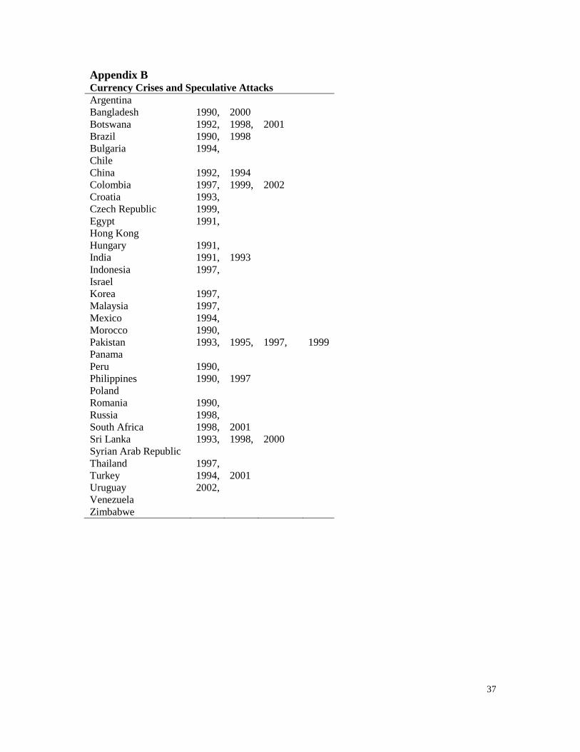
Appendix B Currency Crises and Speculative Attacks Argentina Bangladesh 1990, 2000 Botswana 1992, 1998, 2001 Brazil 1990, 1998 Bulgaria 1994, Chile China 1992, 1994 Colombia 1997, 1999, 2002 Croatia 1993, Czech Republic 1999, Egypt 1991, Hong Kong Hungary 1991, India 1991, 1993 Indonesia 1997, Israel Korea 1997, Malaysia 1997, Mexico 1994, Morocco 1990, Pakistan 1993, 1995, 1997, 1999 Panama Peru 1990, Philippines 1990, 1997 Poland Romania 1990, Russia 1998, South Africa 1998, 2001 Sri Lanka 1993, 1998, 2000 Syrian Arab Republic Thailand 1997, Turkey 1994, 2001 Uruguay 2002, Venezuela Zimbabwe