intermediate methods in observational epidemiology 2008 confounding - ii
Post on 19-Dec-2015
217 views
TRANSCRIPT

Intermediate methods in observational epidemiology
2008
Confounding - II

2110750022110500Total
4030752510040065+
18774251010100<65
Mort. (%)
No. dths
Pop. Mort.
(%)No. dths
Pop. Age
Age as a confounding variable
Unexposed Exposed

2110750022110500Total
4030752510040065+
18774251010100<65
Mort. (%)
No. dths
Pop. Mort.
(%)No. dths
Pop. Age
Age as a confounding variable
AgeDifferent distributions between the groups
Unexposed Exposed

2110750022110500Total
4030752510040065+
18774251010100<65
Mort. (%)
No. dths
Pop. Mort.
(%)No. dths
Pop. Age
Age as a confounding variable
AgeDifferent distributions between the groups
ANDAssociated with mort. (older ages have >mort.)
Unexposed Exposed

2110750022110500Total
4030752510040065+
18774251010100<65
Mort. (%)
No. dths
NMort.
(%)No. dths
N Age
Age as a confounding variable
Relative RiskUNADJUSTED= 21% / 22%= 0.95
Unexposed Exposed

Direct Adjustment
• Create a standard population

Standard P
opulation O
ptions
1) Easiest: Sum the number of personsin each stratum
1000500500Total
4757540065+
525425100<65
StandPopExposedUnexp.
Groups
Age
2110750022110500Total
4030752510040065+
18774251010100<65
Mort (%)
No. dths
N Mort (%)
No. dths
N
ExposedUnexposed
Age

144500500Total
[400 x 75]/[400 + 75]= 637540065+
[100 x 425]/[100 + 425]= 81
425100<65
Stand. Pop. (minimum variance)
ExposedUnexp
Groups
Age
Standard Population Options2. Minimum Variance Method: Useful when the sample sizes are small
(variance of adjusted rates is minimized): Wi= [nAi x nBi] / [nAi + nBi]
2110750022110500Total
4030752510040065+
18774251010100<65
Mort (%)
No. dths
N Mort (%)
No. dths
N
ExposedUnexposed
Age
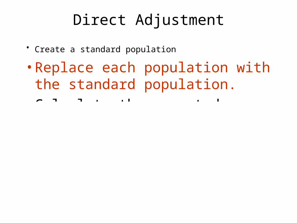
• Create a standard population
• Replace each population with the standard population.
• Calculate the expected number of events in each age group, using the true age-specific rates and the standard population for each age group.
Direct Adjustment

500500Total
40752540065+
1842510100<65
Mort. (%)
Pop. Mort.
(%)Pop. Age
Age as a confounding variable
Unexposed Exposed

144144Total
4063256365+
18811081<65
Mort. (%)
Std pop
Mort.
(%)Std pop
Age
Age as a confounding variable
Unexposed Exposed

• Create a standard population • Replace each population with the standard
population.
• Calculate the expected number of events in each age category, using the true age-specific rates and the standard population for each age group.
Direct Adjustment

144144Total
4063 x .40= 25632563 x .25= 166365+
1881 x .18= 15811081 x .10= 881<65
Mort. (%)
Expected No. of deaths
Std pop
Mort. (%)
Expected No. of deaths
Std pop
ExposedUnexposed
Age
Age as a confounding variable
2110750022110500Total
4030752510040065+
18774251010100<65
Mort (%)
No. dths
N Mort (%)
No. dths
N
ExposedUnexposed
Age

• Create a standard population
• Replace each group with the standard population
• Calculate the expected number of events in each age group, using the true age-specific rates and the standard population for each age group
• Sum up the total number of events in each age category for each group, and divide by the total standard population to calculate the age-adjusted rates
Direct Adjustment

4014424144Total
4063 x .40= 25632563 x .25= 166365+
1881 x .18= 15811081 x .10= 881<65
Mort. (%)
Expected No. of deaths
Std pop
Mort. (%)
Expected No. of deaths
Std pop
ExposedUnexposed
Age
Age as a confounding variable
Age-Adjusted Mortality Rates Unexposed: [24 / 144] x 100= 16.7%
Exposed: [40 / 144] x 100= 27.8%
Relative Risk= 27.8% / 16.7%= 1.7

Example of direct adjustment when the outcome is continuous
No additive interaction
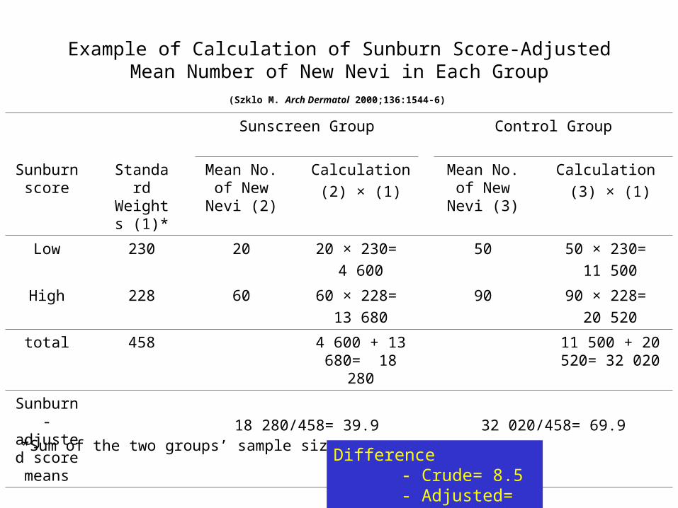
Example of Calculation of Sunburn Score-Adjusted Mean Number of New Nevi in Each Group
Sunscreen Group Control Group
Sunburn score
Standard Weights
(1)*
Mean No. of New Nevi (2)
Calculation
(2) × (1)
Mean No. of New Nevi
(3)
Calculation
(3) × (1)
Low 230 20 20 × 230=
4 600
50 50 × 230=
11 500
High 228 60 60 × 228=
13 680
90 90 × 228=
20 520
total 458 4 600 + 13 680= 18 280
11 500 + 20 520= 32 020
Sunburn-adjusted
score means
18 280/458= 39.9 32 020/458= 69.9
*Sum of the two groups’ sample sizesDifference
- Crude= 8.5- Adjusted= 30.0
(Szklo M. Arch Dermatol 2000;136:1544-6)

Assumptions when adjusting
• Rates are uniform within each stratum (for example, age category--- i.e, age-specific rates are the same for all ages included in each age category, e.g., 25-29 years). – If assumption not true: residual confounding
• There is a uniform difference (absolute or relative) in the age-specific rates between the groups under comparison. – If assumption not true: interaction

Breast Cancer Incidence Rates, USA, SEER, 1973-77
White women Black Women
AGE Pop’n
(in 1000)
% of total
pop’n
Rate (per
100,000)
Pop’n (in
1000)
% of total
pop’n
Rate (per
100,000) 20-29 7,210 26 4.4 955 32 5.7 30-39 5,268 19 38.9 639 21 49.8 40-49 4,786 17 141.5 527 17 121.4 50-59 4,831 17 212.1 452 15 174.9 60-69 3,543 13 267.5 305 10 209.8 70-79 2,299 8 320.2 148 5 264.2 Total 27,937 100 3,026 100 Crude Rate 129.7 93.7
Age-Adjusted Rate*
108.5 93.7
(*Using Black Women as the Standard Population)
W < B

Breast Cancer Incidence Rates, USA, SEER, 1973-77
White women Black Women
AGEPop’n
(in 1000)
% oftotal
pop’n
Rate(per
100,000)
Pop’n(in
1000)
% oftotal
pop’n
Rate(per
100,000)20-29 7,210 26 4.4 955 32 5.730-39 5,268 19 38.9 639 21 49.840-49 4,786 17 141.5 527 17 121.450-59 4,831 17 212.1 452 15 174.960-69 3,543 13 267.5 305 10 209.870-79 2,299 8 320.2 148 5 264.2Total 27,937 100 3,026 100Crude Rate 129.7 93.7Age-AdjustedRate*
108.5 93.7
(*Using Black Women as the Standard Population) W > B

40
WW
BW
Age (years)
Bre
ast
Can
cer
Inci
denc
e R
ates
Interaction between age and ethnic background
“cross-over”

Adjustment and Interaction
Age A B
N Rate (%)
N Rate (%)
ARexp
RR
<50 100 20 200 10 10% 2.00
50+ 200 50 100 40 10% 1.25
• ARs are the same, butRR’s are different
Multiplicative interaction

When ABSOLUTE differences (ATTRIBUTABLE RISKS IN EXPOSED) are homogeneous, adjusted ARexp is the
same regardless of standard population
Age A B N Rate
(%) N Rate
(%)
ARexp
RR <50 100 20 200 10 10% 2.00 50+ 200 50 100 40 10% 1.25
Standard Populations Age Older Younger Minimum
variance <50 200 1800 66.7 50+ 1800 200 66.7
A B A B A B Adj. Rate 47% 37% 23% 13% 35% 25%
ARexp 10% 10% 10% RR 1.3 1.8 1.4

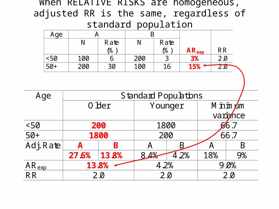
Adjustment and Interaction
Age A B
N Rate (%)
N Rate (%)
ARexp
RR
<50 100 6 200 3 3% 2.0
50+ 200 30 100 16 15% 2.0
• RRs are the same, butARexp’s are different
Additive interaction

When RELATIVE RISKS are homogeneous, adjusted RR is the same, regardless of standard population
Standard Populations Age Older Younger Minimum
variance <50 200 1800 66.7 50+ 1800 200 66.7
A B A B A B Adj. Rate 27.6% 13.8% 8.4% 4.2% 18% 9%
ARexp 13.8% 4.2% 9.0% RR 2.0 2.0 2.0
Age A B N Rate
(%) N Rate
(%)
ARexp
RR <50 100 6 200 3 3% 2.0 50+ 200 30 100 16 15% 2.0

Mantel-Haenszel Formula for Calculation of Adjusted Odds Ratios
Exposure Cases Controls
Yes ai bi
No ci di
Ni
O R
a dN
b cN
M Hi
i i
i
i i
ii
=
a d
b c
b c
Nb c
N
O R w
w
i i
i i
i i
ii
i i
ii
ii
i
ii
=
b cb c
a dN
b cN
i i
i i
i i
ii
i i
ii
Thus, the ORMHis a weighted average of stratum-specific ORs(ORi), with weights equal to each stratum’s:
wb cNii i
i
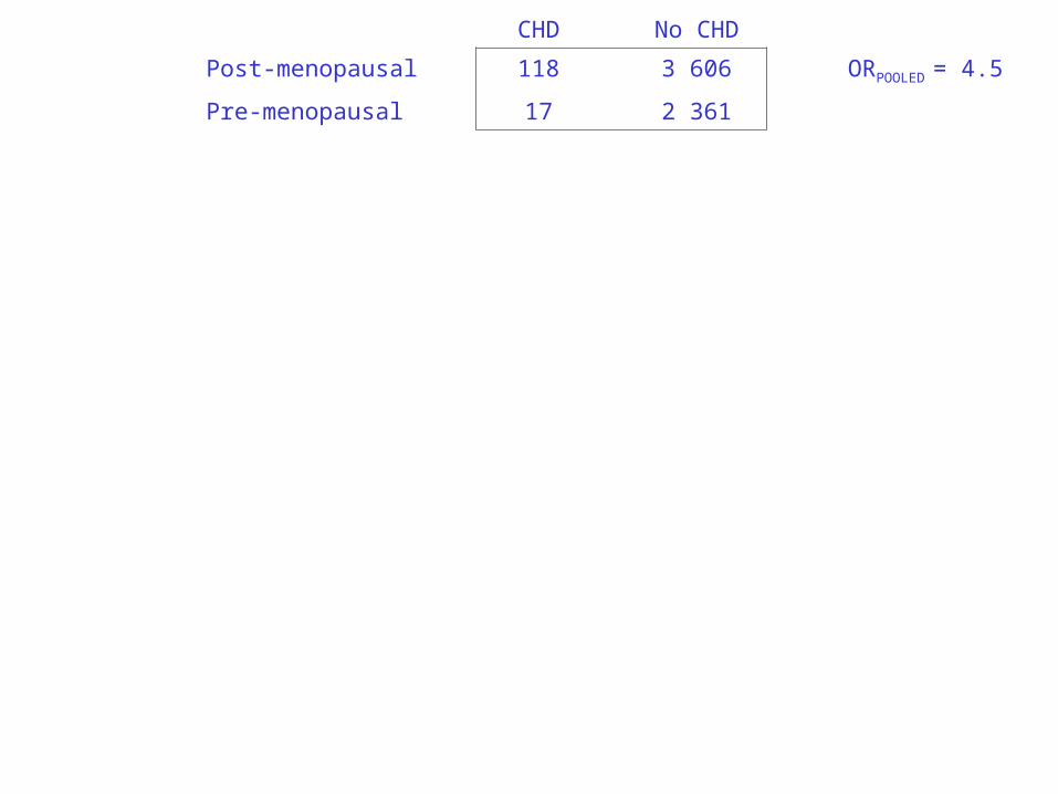
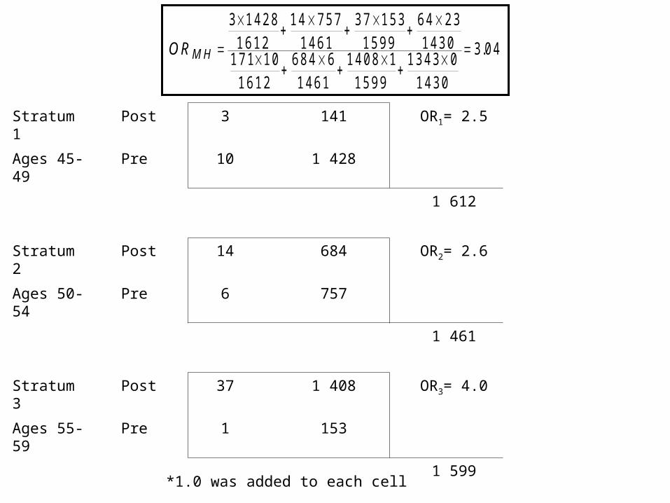
CHD No CHD
Post-menopausal 118 3 606 ORPOOLED = 4.5
Pre-menopausal 17 2 361

Stratum 1 Post 3 141 OR1= 2.5
Ages 45-49 Pre 10 1 428
1 612
Stratum 2 Post 14 684 OR2= 2.6
Ages 50-54 Pre 6 757
1 461
Stratum 3 Post 37 1 408 OR3= 4.0
Ages 55-59 Pre 1 153
1 599
Stratum 4 Post 64 1 343 OR4= 1.2*
Ages 60-64 Pre 0 23
1 430
CHD No CHD
Post-menopausal 118 3 606 ORPOOLED = 4.5
Pre-menopausal 17 2 361
*1.0 was added to each cell
Variable to be adjusted for in
the outside stubMain
varia
ble
of in
tere
st in
the
inside
stub

Stratum 1 Post 3 141 OR1= 2.5
Ages 45-49 Pre 10 1 428
1 612
Stratum 2 Post 14 684 OR2= 2.6
Ages 50-54 Pre 6 757
1 461
Stratum 3 Post 37 1 408 OR3= 4.0
Ages 55-59 Pre 1 153
1 599
Stratum 4 Post 64 1 343 OR4= 1.2*
Ages 60-64 Pre 0 23
1 430*1.0 was added to each cell
Stratum 1 Post 3 141 OR1= 2.5
Ages 45-49 Pre 10 1 428
1 612
Stratum 2 Post 14 684 OR2= 2.6
Ages 50-54 Pre 6 757
1 461
Stratum 3 Post 37 1 408 OR3= 4.0
Ages 55-59 Pre 1 153
1 599
Stratum 4 Post 64 1 343 OR4= 1.2*
Ages 60-64 Pre 0 23
1 430
O R M H
3 1 4 2 81 6 1 2
1 4 7 5 71 4 6 1
3 7 1 5 31 5 9 9
6 4 2 31 4 3 0
1 7 1 1 01 6 1 2
6 8 4 61 4 6 1
1 4 0 8 11 5 9 9
1 3 4 3 01 4 3 0
3 0 4.
*1.0 was added to each cell

Stratum 1 Post 3 141 OR1= 2.5
Ages 45-49 Pre 10 1 428
1 612
Stratum 2 Post 14 684 OR2= 2.6
Ages 50-54 Pre 6 757
1 461
Stratum 3 Post 37 1 408 OR3= 4.0
Ages 55-59 Pre 1 153
1 599
Stratum 4 Post 64 1 343 OR4= 1.2*
Ages 60-64 Pre 0 23
1 430
O R M H
3 1 4 2 81 6 1 2
1 4 7 5 71 4 6 1
3 7 1 5 31 5 9 9
6 4 2 31 4 3 0
1 7 1 1 01 6 1 2
6 8 4 61 4 6 1
1 4 0 8 11 5 9 9
1 3 4 3 01 4 3 0
3 0 4.
ORMZ = Weighted average= 3.04
Is this weighted average
representative of the OR in this stratum?
*1.0 was added to each cell

Stratum 1 Post 3 141 OR1= 2.5
Ages 45-49 Pre 10 1 428
1 612
Stratum 2 Post 14 684 OR2= 2.6
Ages 50-54 Pre 6 757
1 461
Stratum 3 Post 37 1 408 OR3= 4.0
Ages 55-59 Pre 1 153
1 599
Report the OR separately for age group 60-64
Stratum 4 Post 64 1 343 OR4= 1.2*
Ages 60-64 Pre 0 23
1 430
Calculate the MH-adjusted OR for these 3 (relatively) homogeneous age groups and…
O R M H
3 1 4 2 8
1 6 1 2
1 4 7 5 7
1 4 6 1
3 7 1 5 3
1 5 9 91 7 1 1 0
1 6 1 2
6 8 4 6
1 4 6 1
1 4 0 8 1
1 5 9 9
2 8 3.
*1.0 was added to each cell

Men Cases Controls
Exposed 20 5 OR= 4.75
Unexposed 80 95
100 100 200
Women
Exposed 10 25 OR= 0.33
Unexposed 90 75
100 100 200
O R M H
2 0 9 5
2 0 0
1 0 7 5
2 0 08 0 5
2 0 0
9 0 2 5
2 0 0
1 0.
Does an ORMH= 1.0 properly characterize the relationship of the exposure to the disease in this study population? NO
A MORE DRAMATIC EXAMPLE

Stratification Methods
• Advantages
– Easy to understand and compute
– Allow simultaneous assessment of interaction
• Disadvantages
– Cannot handle a large number of variables
– Each calculation requires a rearrangement of tables

Stratification Methods
• Advantages
– Easy to understand and compute
– Allow simultaneous assessment of interaction
• Disadvantages
– Cannot handle a large number of variables
– Each calculation requires a rearrangement of tables

Main Variable of Interest: Menopausal Status
Age Menopausal?
Cases Contls
45-49 Pre
Post
50-54 Pre
Post
55-59 Pre
Post
60-64 Pre
Post
Main Variable of Interest: Age
Menopausal? Age Cases Contls
Pre 45-49
50-54
55-59
60-64
Post 45-49
50-54
55-59
60-64

Types of confounding
• Positive confoundingWhen the confounding effect results in an overestimation
of the magnitude of the association (i.e., the crude OR estimate is further away from 1.0 than it would be if confounding were not present).
• Negative confoundingWhen the confounding effect results in an
underestimation of the magnitude of the association (i.e., the crude OR estimate is closer to 1.0 than it would be if confounding were not present).

10.1 10
Odds Ratio
3.0
2.0
0.40.3
3.00.7
0.40.7
Type of confounding:Positive Negative
3.0TRUE, UNCONFOUNDED
5.0OBSERVED, CRUDE
x
x
x
x
x ? QUALITATIVE CONFOUNDING
1/3.3=1/2.5=

Confounding is not an “all or none” phenomenon
A confounding variable may explain the whole or just part of the observed association between a given exposure and a given outcome.
• Crude OR=3.0 … Adjusted OR=1.0• Crude OR=3.0 … Adjusted OR=2.0
The confounding variable may reflect a “constellation” of variables/characteristics
– E.g., Occupation (SES, physical activity, exposure to environmental risk factors)
– Healthy life style (diet, physical activity)

Directions of the Associations of the Confounder with the Exposure and the Disease, and Expectation of Change of Estimate with Adjustment (Assume a Direct Relationship Between the Exposure and the Disease,
i.e., Odds Ratio > 1.0 (in Case-Based Control Studies), or Relative Risk > 1.0 (in Case-Cohort Studies)
Association of Exposure with Confounder is
Association of Confounder with Disease is
Type of confounding
Expectation of Change from Unadjusted to Adjusted OR
Direct* Direct* Positive# Unadjusted > Adjusted
Direct* Inverse** Negative## Unadjusted < Adjusted
Inverse** Direct* Positive# Unadjusted > Adjusted
Inverse** Inverse** Negative## Unadjusted < Adjusted
*Direct association: presence of the confounder is related to an increased odds of the exposure or the disease**Inverse association: presence of the confounder is related to a decreased odds of the exposure or the disease#Positive confounding: when the confounding effect results in an unadjusted odds ratio further away from the null hypothesis than the adjusted estimate##Negative confounding” when the confounding effect results in an unadjusted odds ratio closer to the null hypothesis than the adjusted estimate
CONFOUNDING EFFECT IN CASE-CONTROL STUDIES
(Szklo M & Nieto FJ, Epidemiology: Beyond the Basics, Jones & Bartlett, 2nd Edition, 2007, p. 176)

Residual confounding
Controlling for one of several confounding variables does not guarantee that confounding be completely removed.
Residual confounding may be present when:
- The variable that is controlled for is an imperfect surrogate of the true confounder,
- Other confounders are ignored,
- The units of the variable used for adjustment/stratification are too broad
- The confounding variable is misclassified
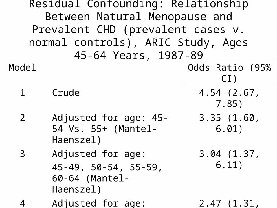
Residual Confounding: Relationship Between Natural Menopause and
Prevalent CHD (prevalent cases v. normal controls), ARIC Study, Ages 45-64 Years,
1987-89Model Odds Ratio (95% CI)
1 Crude 4.54 (2.67, 7.85)
2 Adjusted for age: 45-54 Vs. 55+ (Mantel-Haenszel)
3.35 (1.60, 6.01)
3 Adjusted for age:
45-49, 50-54, 55-59, 60-64 (Mantel-Haenszel)
3.04 (1.37, 6.11)
4 Adjusted for age: continuous (logistic regression)
2.47 (1.31, 4.63)

CONTROLLING FOR CONFOUNDING WITHOUT ADJUSTMENT
Men: Years of Age Women: Years of Age
30-49 50-62 30-49 50-62
Serum Cholesterol
(mg/dL) Incidence Rates per 1,000 Individuals
< 190 38.2 105.7 11.1 155.2
190-219 44.1 187.5 9.1 88.9
220-249 95.0 201.1 24.3 96.3
250+ 157.5 267.8 50.4 121.5
(Truett et al, J Chronic Dis 1967;20:511)

Men: Years of Age Women: Years of Age
30-49 50-62 30-49 50-62
Serum Cholesterol
(mg/dL) Incidence Rates per 1,000 Individuals
< 190 38.2 105.7 11.1 155.2
190-219 44.1 187.5 9.1 88.9
220-249 95.0 201.1 24.3 96.3
250+ 157.5 267.8 50.4 121.5
(Truett et al, J Chronic Dis 1967;20:511)
How to control (“adjust”) with no calculations?- Examine the effect of varying one variable, holding all
other variables “constant” (fixed).
Relationship Between Serum Cholesterol Levels and Risk of Coronary Heart Disease by Age and Sex, Framingham Study, 12-year Follow-up

Men: Years of Age Women: Years of Age
30-49 50-62 30-49 50-62
Serum Cholesterol
(mg/dL) Incidence Rates per 1,000 Individuals
< 190 38.2 105.7 11.1 155.2
190-219 44.1 187.5 9.1 88.9
220-249 95.0 201.1 24.3 96.3
250+ 157.5 267.8 50.4 121.5
(Truett et al, J Chronic Dis 1967;20:511)
Examine the effect of varying one variable, holding allother variables “constant” (fixed). Example: effect of sex,
holding serum cholesterol and age constant

Men: Years of Age Women: Years of Age
30-49 50-62 30-49 50-62
Serum Cholesterol
(mg/dL) Incidence Rates per 1,000 Individuals
< 190 38.2 105.7 11.1 155.2
190-219 44.1 187.5 9.1 88.9
220-249 95.0 201.1 24.3 96.3
250+ 157.5 267.8 50.4 121.5
(Truett et al, J Chronic Dis 1967;20:511)
Examine the effect of varying one variable, holding allother variables “constant” (fixed). Example: effect of
serum cholesterol, holding sex and age constant

Men: Years of Age Women: Years of Age
30-49 50-62 30-49 50-62
Serum Cholesterol
(mg/dL) Incidence Rates per 1,000 Individuals
< 190 38.2 105.7 11.1 155.2
190-219 44.1 187.5 9.1 88.9
220-249 95.0 201.1 24.3 96.3
250+ 157.5 267.8 50.4 121.5
(Truett et al, J Chronic Dis 1967;20:511)
Examine the effect of varying one variable, holding allother variables “constant” (fixed). Example: effect of age,
holding sex and serum cholesterol constant.