Interdecadal changes of the Indian Ocean subtropical dipole mode

Yoko Yamagami • Tomoki Tozuka

Received: 28 January 2014 / Accepted: 26 May 2014 / Published online: 10 June 2014

� Springer-Verlag Berlin Heidelberg 2014

Abstract Using observational data and outputs from an

ocean general circulation model, the interdecadal changes

in the Indian Ocean subtropical dipole (IOSD) are inves-

tigated for the first time. It is found that the frequency of

the IOSD has become higher because of a decreasing trend

in the mixed layer depth (MLD) over the southwestern pole

in January and February. Positive (negative) sea surface

temperature (SST) anomalies associated with the IOSD are

generated when the mixed layer becomes anomalously

shallow (deep). The thinner mixed layer in the recent

decade amplifies this effect and even weak atmospheric

forcing may trigger the IOSD. From a diagnosis of the

Monin–Obukhov depth, it is shown that an increasing trend

of surface heat flux, which is due to the decrease of wind

speed (increase of specific humidity near the sea surface)

associated with the poleward shift of westerly jet in Janu-

ary (the strengthening of Mascarene high in February),

causes the decreasing trend of the MLD. On the other hand,

the smaller amplitude in the recent decades is because the

IOSD starts to develop in December, but the deeper mixed

layer in December in the recent decade provides an unfa-

vorable condition for its development. In addition, the

shallower mixed layer in January and February may also

amplify the negative feedback processes that damp the SST

anomalies. Since no interdecadal changes in interannual

variability of atmospheric forcing corresponding to that in

the IOSD are observed, the interdecadal trend in the MLD

is essential for that of the IOSD.

1 Introduction

Since climate variations in the Indian Ocean have much

impact on the society, many studies have been devoted to

their understanding. The Indian Ocean Dipole (IOD; Saji

et al. 1999) is one of the most dominant modes of climate

variability in the tropical Indian Ocean, and its mechanisms

and climatic impacts have been investigated extensively

(see reviews by Yamagata et al. 2004; Chang et al. 2006).

Recently, its natural decadal variability (Tozuka et al.

2007) and changes under global warming (Zheng et al.

2010, 2013; Cai et al. 2013) have been discussed.

There is another important climate mode in the Indian

Ocean called the Indian Ocean subtropical dipole (IOSD;

Behera and Yamagata 2001). Its positive phase is associ-

ated with positive (negative) SST anomalies in the south-

western (northeastern) part of the southern Indian Ocean.

This phenomenon is strongly locked to seasons; SST

anomalies develop in December and January, peak in

February, and decay afterwards. Earlier studies (Behera

and Yamagata 2001; Suzuki et al. 2004; Hermes and

Reason 2005; Chiodi and Harrison 2007) reported that

anomalous warming (cooling) over the southwestern

(northeastern) pole is mainly due to a decrease (an

increase) in latent heat flux associated with a strengthening

and southward shift of the Mascarene high. However,

Morioka et al. (2010, 2012) recently showed the impor-

tance of mixed layer depth (MLD) anomalies; a change in

the subtropical high suppresses (enhances) latent heat loss

due to a decrease in the specific humidity difference (an

increase in the specific humidity difference and in the near-

surface wind speed) in the southwestern (northeastern)

pole. As a result, the mixed layer becomes thinner (thicker)

than normal. This, in turn, enhances (suppresses) warming

of the mixed layer by climatological shortwave radiation

Y. Yamagami (&) � T. TozukaDepartment of Earth and Planetary Science, Graduate School of

Science, University of Tokyo, 7-3-1 Hongo, Bunkyo-ku,

Tokyo 113-0033, Japan

e-mail: yamagami@eps.s.u-tokyo.ac.jp

123

Clim Dyn (2015) 44:3057–3066

DOI 10.1007/s00382-014-2202-9

and generates the positive (negative) SST anomaly pole.

After reaching the peak, the positive (negative) pole decays

in early austral fall because of the larger (smaller) tem-

perature difference between the mixed layer and entrained

water, and larger (smaller) latent heat loss due to the larger

(smaller) specific humidity difference and the decreased

stability (wind speed) near the surface. It is also suggested

that the modulation in the subtropical high is linked with

ENSO and/or climate modes in the high latitudes such as

the Southern Annular Mode (SAM) and the Antarctic

Circumpolar Waves (Fauchereau et al. 2009; Hermes and

Reason 2005; Terray 2011; Morioka et al. 2013).

Since the IOSD may potentially influence precipitation

anomalies over southern Africa (Reason 1998, 2001; Be-

hera and Yamagata 2001; Yuan et al. 2014), the Indian

summer monsoon (Terray et al. 2003), ENSO (Boschat

et al. 2013), and the IOD (Fischer et al. 2005), how the

occurrence of the IOSD varies and/or changes on decadal-

to-intedecadal time scales is an important issue. However,

this has not been addressed so far and this is the motive of

this study.

Using observation data and outputs from an ocean

general circulation model (OGCM), we have investigated

the interdecadal changes in the IOSD. This paper is orga-

nized as follows. A brief description of the data and an

OGCM is given in the next section. In Sect. 3, we first

describe the interdecadal changes seen in the observed and

simulated IOSD. Then, we discuss possible mechanisms of

such a change and its relation with the other climate modes

such as ENSO by examining changes in MLD and sea level

pressure (SLP). The final section summarizes the main

results.

2 Data and model

We use the monthly mean observed SST data from the

Hadley Centre sea ice and sea surface temperature (Had-

ISST; Rayner et al. 2003) with a horizontal resolution of

1� 9 1�. We analyzed the period of 1980–2012, because

there were few observations in the southern Indian Ocean

until the 1970s. Based on this SST data, we calculated the

Nino 3.4 index, which is computed by taking an average of

SST anomalies over the Nino 3.4 region (120�W–170�W,

5�S–5�N). We also use SLP, wind, and specific humidity at

2 m heigth data from the National Centers for Environ-

mental Prediction–National Center for Atmospheric

Research (NCEP–NCAR) reanalysis dataset (Kalnay et al.

1996) from 1980 to 2012 on a 2.5� 9 2.5� grid. Using this

SLP data, the index of SAM (e.g., Thompson and Wallace

2000), which is referred as the SAM index hereafter, is

defined as SAM index ¼ SLPA�40�S � SLPA�

70�S. Here,

SLPA�40�S and SLPA�

70�S are normalized monthly SLP

anomalies zonaly averaged in 40�S and 70�S, respectively(Nan and Li 2003). For the climatological MLD, the

observational data prepared by de Boyer Montequt et al.

(2004) is used.

Due to the lack of interannual subsurface ocean data in the

earlier period, we also use outputs from an OGCM. The

ocean model is based on the Modular Ocean Model, version

3.0 (MOM 3.0), developed at the National Oceanic and

Atmospheric Administration/Geophysical Fluid Dynamics

Laboratory (Pacanowski and Griffies 1999). The model

covers the global ocean from 65�S to 30�N, and has a hori-

zontal resolution of 0.5� 9 0.5� and 25 levels in the verticalwith eight levels in the upper 100 m, and 10 m interval in the

upper 50 m. Near the northern/southern boundary (poleward

of 27�N/62�S), sponge layers are introduced to reduce the

effect of the artificial northern/southern coast; the lateral

eddy viscosity and diffusivity are increased and the tem-

perature and salinity are relaxed to the monthly mean cli-

matology (Levitus and Boyer 1994; Levitus et al. 1994). The

model is first spun up for 20 years by the monthly mean

climatology of the NCEP/NCAR reanalysis dataset. Then,

the model is integrated for 59 years from 1950 to 2008 using

the daily mean data and we only analyze the outputs after

1980. The model can reproduce the realistic SST variability

associated with the IOSD (Morioka et al. 2010).

3 Results

3.1 Interdecadal changes in the IOSD

To examine how the IOSD has changed interdecadally, we

need to introduce an IOSD index. For this purpose, we

have applied empirical orthogonal function (EOF) analysis

to detrended SST anomalies of all the months over the

southern Indian Ocean (30�E–120�E, 50�S–10�S). Figure 1

shows spatial patterns of the first EOF mode of observed

and simulated SST anomalies explaining 20.6 and 19.5 %

of the total variance, respectively. Since similar southwest–

northeast oriented dipoles are captured by both of them, the

model has good skill in simulating SST anomalies associ-

ated with the IOSD.

Then, we define the IOSD index as the difference in SST

anomalies between the southwestern (48�E–68�E, 47�S–37�S) and northeastern (85�E–105�E, 35�S–25�S) poles, andthe time series of the index is given in Fig. 2a. Since the EOF

is affected by orthogonality, we have introduced the IOSD

index, but the correlation coefficient between the principal

component of the first EOF mode and the IOSD index in the

observation and themodel are high (r[ 0.84) and our results

are qualitatively the same even if we use the principal

component. Also, we have confirmed that our results are not

very sensitive to slight shifts in the location of the two boxes,

3058 Y. Yamagami, T. Tozuka

123

and the index is generally capturing dipole patterns, not

merely capturing a very strong pole in the southwest or

northeast. The correlation coefficient between the observed

and modeled indices over all the months is 0.81, which is

significant at 95 % confidence level and indicative of a high

skill in simulating the IOSD. The IOSD index undergoes

large interannual variations, but it is interesting to note that

the period seems to become shorter and the amplitude seems

to become smaller in the recent decade.

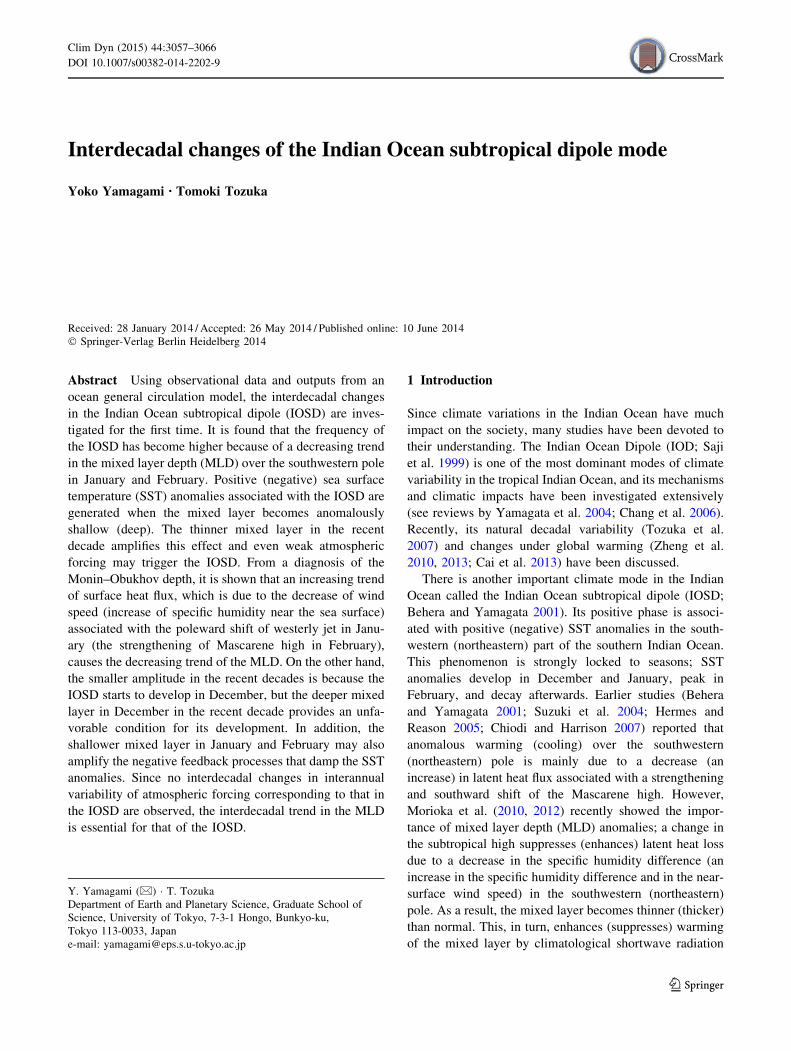
To check a possible change in dominant periods of the

IOSD more clearly, we have applied wavelet analysis

(Torrence and Compo 1999) to the IOSD index (Fig. 3a,

b). Both wavelet spectra show the same trend; the peak is

found around 3–4 years before the 1990s, but the peak

gradually shifts toward the shorter period and is seen

around 1–2 years in the recent decade. Also, we note that

the power spectra become weaker in the 2000s.

3.2 Mechanism

To determine why the period and amplitude of the IOSD

have changed, we consider the temperature balance within

the mixed layer

oTm

ot¼ Qnet � qd

qCpH� um � rTm � DT

Hwe þ res: ð1Þ

Here, the first term on the right hand side of Eq. (1)

indicates the contribution from surface heat flux, where

Qnet is net surface heat flux, qd is downward solar insola-

tion penetrating through the mixed layer bottom, q(=1,027 kg m-3) is the density of the seawater, cp is the

specific heat of the seawater, and H is the MLD, which is

defined as a depth at which the temperature is 0.8 �C lower

than the SST (our results are qualitatively the same even if

we use 0.2 �C criterion). The second term represents hor-

izontal advection in the mixed layer, where Tm and um are

temperature and horizontal velocity averaged in the mixed

layer, respectively. The third term is the contribution from

the entrainment, where DT is the difference between the

temperature of the mixed layer water and the water

entrained from below the mixed layer, and we is entrain-

ment velocity. The residual term consists of diffusion,

detrainment and other processes. When the IOSD is in its

growing phase, the surface heat flux term is dominant and

the contribution from the other oceanic terms is smaller

(Morioka et al. 2010, 2012). The surface heat flux term can

be decomposed as

Fig. 1 Spatial patterns of the

first EOF mode of SST

anomalies from a HadISST and

b MOM3 (in �C). Contourinterval is 0.1 �C. Percentage of

the explained variance is also

shown. The rectangular boxes

denote the southwestern pole

(48�E–68�E, 47�S–37�S) andnortheastern pole (85�E–105�E,35�S–25�S) of the IOSD

(a) (b)

Fig. 2 a Time series of the IOSD index (in �C) from the HadISST

(red) and MOM3 (blue). The horizontal lines indicate 1.5 standard

deviations of the IOSD index obtained from the HadISST (solid) and

MOM3 (dashed). The time series are smoothed using a 3-month

running mean. b Normalized time series of the Nino 3.4 index (red),

IOSD index (blue), and SAM index (green) from 1980 to 2012. The

time series are smoothed using a 5-month running mean

Interdecadal changes 3059

123

dQnet � qd

qCpH

� �� d

Q

qCpH

� �� �¼ dQ

qCp�H� dH �Q

qCp�H2

þ res;

ð2Þ

where � � �ð Þ is the monthly mean climatology, d � � �ð Þ indi-cates a deviation from the monthly climatology, and

Q ¼ Qnet � qd.

As shown by Morioka et al. (2010, 2012), the second

term on the right hand side of Eq. (2) is dominant during

the developing phase of the IOSD and the MLD anomaly is

essential. For the interdecadal change, however, a change

in the climatological MLD and/or surface heat flux may be

of importance. In particular, since the denominator of the

second term contains a square of the climatological MLD,

the magnitude of the second term is sensitive to a change in

the climatological MLD.

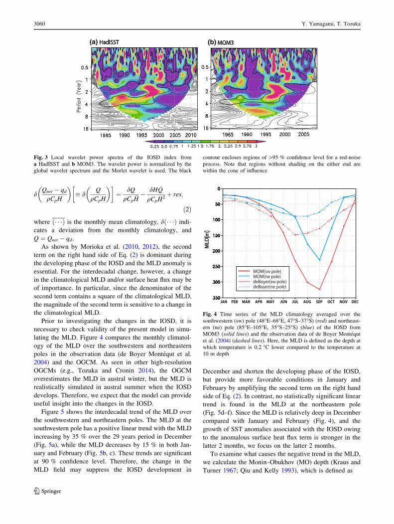
Prior to investigating the changes in the IOSD, it is

necessary to check validity of the present model in simu-

lating the MLD. Figure 4 compares the monthly climatol-

ogy of the MLD over the southwestern and northeastern

poles in the observation data (de Boyer Montequt et al.

2004) and the OGCM. As seen in other high-resolution

OGCMs (e.g., Tozuka and Cronin 2014), the OGCM

overestimates the MLD in austral winter, but the MLD is

realistically simulated in austral summer when the IOSD

develops. Therefore, we expect that the model can provide

useful insight into the changes in the IOSD.

Figure 5 shows the interdecadal trend of the MLD over

the southwestern and northeastern poles. The MLD at the

southwestern pole has a positive linear trend with the MLD

increasing by 35 % over the 29 years period in December

(Fig. 5a), while the MLD decreases by 15 % in both Jan-

uary and February (Fig. 5b, c). These trends are significant

at 90 % confidence level. Therefore, the change in the

MLD field may suppress the IOSD development in

December and shorten the developing phase of the IOSD,

but provide more favorable conditions in January and

February by amplifying the second term on the right hand

side of Eq. (2). In contrast, no statistically significant linear

trend is found in the MLD at the northeastern pole

(Fig. 5d–f). Since the MLD is relatively deep in December

compared with January and February (Fig. 4), and the

growth of SST anomalies associated with the IOSD owing

to the anomalous surface heat flux term is stronger in the

latter 2 months, we focus on the latter 2 months.

To examine what causes the negative trend in the MLD,

we calculate the Monin–Obukhov (MO) depth (Kraus and

Turner 1967; Qiu and Kelly 1993), which is defined as

Fig. 4 Time series of the MLD climatology averaged over the

southwestern (sw) pole (48�E–68�E, 47�S–37�S) (red) and northeast-

ern (ne) pole (85�E–105�E, 35�S–25�S) (blue) of the IOSD from

MOM3 (solid lines) and the observation data of de Boyer Montequt

et al. (2004) (dashed lines). Here, the MLD is defined as the depth at

which temperature is 0.2 �C lower compared to the temperature at

10 m depth

(a) (b)

Fig. 3 Local wavelet power spectra of the IOSD index from

a HadISST and b MOM3. The wavelet power is normalized by the

global wavelet spectrum and the Morlet wavelet is used. The black

contour encloses regions of[95 % confidence level for a red-noise

process. Note that regions without shading on the either end are

within the cone of influence

3060 Y. Yamagami, T. Tozuka

123

HMO ¼ m0u3� þ

agqCp

Z0

�HMO

qðzÞdz

264

375,

ag2qCp

ðQnet � qdÞ:

ð3Þ

Here, m0ð¼ 0:5Þ is a coefficient for the efficiency of

wind stirring, u� is frictional velocity, defined by

u� � qaCDu210=q

� �1=2, where qað¼ 1:3kg m�3Þ is the den-

sity of air, CDð¼ 0:00125Þ is a drag coefficient, and u10 is

wind speed at 10-m height. Also, að¼ 0:00025Þ is the

thermal expansion coefficient of the seawater, and

q zð Þ ¼ q 0ð Þ 0:62 exp z=1:5ð Þ þ 0:38 exp z=20ð Þ½ �ð Þ is down-

ward solar insolation (Paulson and Simpson 1977). We can

decompose the interannual anomaly of the MO depth as

d HMOð Þ � dm0u

3� þ q�Q�

� �� �

¼m0d u3�

� �Q�

þ dq�Q�

�dQ� m0u3� þ q�

�

Q�� �2 þ res;

ð4Þ

where Q� ¼ 2qCp

� ��1ag Qnet � qdð Þ

� is the effective

buoyancy forcing and q� ¼ qCp

� ��1ag

R 0

�HMOq zð Þdz

� is

the effective penetrative shortwave radiation (Morioka

et al. 2012).

In agreement with the simulated MLD, the MO depth

in January and February indicates a decreasing trend

(Fig. 6a, d). When each term in Eq. (4) is calculated

(Fig. 6b, e), it is found that the third term, i.e. the

contribution from the deviation in the net surface heat

flux, is dominant. This result indicates that the inter-

decadal trend of the MO depth is mainly due to that of

the net surface heat flux (Fig. 6c, f), and the stabilizing

effect of surface heating is causing the MLD to become

shallower. We note that the larger net surface heat flux

in the recent decade may also favor the development of

the IOSD by amplifying the second term on the right

hand side of Eq. (2).

To investigate the cause of the surface heat flux trends,

the spatial patterns of linear trends of the MLD, heat flux,

(a)

(d)

(c)(b)

(e) (f)

Fig. 5 Time series of the MLD averaged over the southwestern pole

in a December, b January, and c February (in m). d–f As in a–c, butfor the northeastern pole. The dashed lines mean a significant trend

exceeding 90 % confidence level by the two-tailed t test. The time

series are smoothed using a 3-year running mean

Interdecadal changes 3061

123

wind vector, and wind speed or specific humidity is cal-

culated (Figs. 7, 8). Figures 7a and 8a show spatial patterns

of linear trends in the MLD in January and February,

respectively. Although positive trends are found to the

south of 42�S in the southeastern Indian Ocean (Salle et al.

2010) and over the Seychelles Dome region in the south-

western tropical Indian Ocean (Tozuka et al. 2010), nega-

tive trends are prevalent including the southwestern pole of

the IOSD.

The net surface heat flux has a positive trend over

the southwestern pole (Figs. 7b, 8b) and it is dominated

by that in latent heat flux (Figs. 7c, 8c), owing to a

decrease in the wind speed (specific humidity) in Jan-

uary (February) (Figs. 7d, 8d). The westerly wind has

weakened in the 35�S–50�S band, but it has become

stronger in the high latitudes in January (Fig. 7d). These

trends are consistent with the poleward shift of the

westerly jet under global warming (Kushner et al. 2001;

Yin 2005). On the other hand, the Mascarene high is

strengthening (Fig. 8d) in February. The increase of

northerly wind enhances the transport of the moist and

warm air from the low latitudes and suppresses the

evaporation.

3.3 Possible role of the atmospheric forcing

Although we have focused our attention on oceanic vari-

ability in seeking the cause of interdecadal changes in the

dominant frequency of the IOSD, a change in frequency of

atmospheric forcing may also lead to the interdecadal

changes in the IOSD. This is because the IOSD is known to

be closely linked with variability in the Mascarene high

(Behera and Yamagata 2001) and SLP anomalies in the

southern Indian Ocean are shown to undergo interdecadal

changes (Allan et al. 1995; Reason et al. 1996).

To capture the dominant mode of atmospheric vari-

ability in the southern Indian Ocean, we have applied the

EOF analysis to SLP anomalies. Figure 9a shows the

spatial pattern of the first EOF mode, which explains

37.1 % of the total variance. The spatial pattern resembles

that of composite diagrams of SLP anomalies in the IOSD

years shown by Morioka et al. (2010). Based on the EOF

analysis, we then calculate area-averaged SLP anomalies

in a box region (68�E–88�E, 52�S–42�S) to represent

temporal variability of SLP anomalies. Figure 9b shows

the principal component of the first EOF mode as well as

the SLP index defined above. These two time series are

(a) (b)

(e)

(c)

(f)(d)

Fig. 6 a, d Time series of the

Monin–Obukhov (MO) depth

(in m) over the southwestern

pole. b, e Time series of the MO

depth anomalies and

contribution from wind stirring

(red), shortwave radiation

(blue), net surface heat flux

(green), and residual (yellow)

(in m). c, f Time series of the

net surface heat flux (in

W m-2). Figures on the upper

(lower) row are for January

(February). A dashed line in

each figure signifies a

significant trend exceeding

90 % confidence level by the

two-tailed t test. The time series

are smoothed using a 3-year

running mean

3062 Y. Yamagami, T. Tozuka

123

highly correlated with each other with a correlation

coefficient of 0.94, which is significant at 95 % confi-

dence level.

It is interesting to note that the correlation coefficient

between the principal component of the first EOF mode

and the IOSD index shown in Fig. 9b is high during the

earlier period; the correlation coefficient is about 0.8 in the

1980s, but decreases to about -0.2 in the 2000s (Fig. 10a).

The correlation coefficient between the SLP index and the

IOSD index also decreases from the 1980s to the 2000s.

This infers that strong atmospheric forcing was necessary

in the earlier period to trigger the IOSD when the MLD

was relatively deep. On the other hand, the MLD is rela-

tively shallow in the latter period and even small anomalies

in the atmospheric circulation may induce the IOSD.

Figure 10b shows the wavelet power spectrum of the

SLP index. Statistically significant peaks are found only in

periods shorter than 2 years throughout the 1980–2008

period and there is no shift in the dominant period. Hence,

a change in frequency of atmospheric forcing is not the

cause of the interdecadal change in the IOSD.

Since the center of atmospheric variability may shift on

interdecadal time-scales and a single SLP index may not be

able to capture interdecadal changes, we have also checked

the correlation coefficient between SLP anomalies averaged

over 20� longitude 9 10� latitude boxes in different parts ofthe southern Indian Ocean and the IOSD index. It is found

that all of these correlation coefficients show similar ten-

dency. Also, wavelet power spectra of each SLP time series

have been calculated, but no interdecadal shift in the domi-

nant period is found (figure not shown). Therefore, the

interdecadal change in the dominant frequency of the IOSD

does not stem from that of the Mascarene high.

As reported by McPhaden (2012), ENSO has undergone

a significant change in the recent decade (Fig. 2b). Since

an atmospheric teleconnection from ENSO is considered as

one of the triggers of the IOSD (Morioka et al. 2013), such

a change in ENSO may modulate the IOSD. However,

there was no interdecadal change in the dominant fre-

quency of SLP anomalies over the southern Indian Ocean.

Thus, we may rule out the possibility of interdecadal

change in ENSO as the root cause of the interdecadal

change in the dominant frequency of the IOSD. For the

same reason, the interdecadal changes in the IOSD are not

due to the interdecadal change in the dominant frequency

of the SAM.

(a) (b)

(C) (d)

Fig. 7 Spatial patterns of linear trends in a the MLD (in m/29 years),

b the net surface heat flux (in Wm-2/29 years), c latent heat flux (in

Wm-2/29 years) and d wind speed (in ms-1/29 years) in January.

Contour interval is a 5 m/29 years, b, c 5 Wm-2/29 years, and

d 1 ms-1/29 years. Trends significant at 90 % confidence level by the

two-tailed t test are shaded. The linear trend is calculated using the

time series of each variable smoothed by 3-year running mean.

Vectors in d indicate linear trends of wind vectors and only those

significant at 90 % confidence level by two-tailed t test are shown

Interdecadal changes 3063

123

Also, we note that the IOSD does not develop even

when large SLP anomalies exist (1988/1989, 2001/2002,

2004/2005, and 2005/2006) (Fig. 9b). It is found that this

may be due to the fact that the sign of MLD anomalies at

the onset stage is unfavorable for the growth of SST

anomalies associated with the IOSD.

4 Conclusions

Using observational data and outputs from an OGCM, the

interdecadal changes of the IOSD are investigated for the first

time. The wavelet power spectrum of the IOSD index implies

that its frequency is becoming higher and its amplitude is

(C)

(a) (b)

(d)

Fig. 8 a–c Same as Fig. 7 but for February. d As in Fig. 7d but with linear trends in specific humidity (shading)

(a) (b)

Fig. 9 a Spatial pattern of the first EOF mode of SLP anomalies (in

hPa). Percentage of the explained variance is also shown. The box is

used to calculate the SLP index. b Normalized DJF-mean time series

of the SLP index (black), the principal component of the first EOF

mode (PC1, red), and the IOSD index (blue)

3064 Y. Yamagami, T. Tozuka

123

getting smaller in the recent years. The shorter period is due to

a decreasing trend in the MLD; positive (negative) SST

anomalies associated with the IOSD develop when the mixed

layer becomes anomalously shallow (deep) and the warming

of the mixed layer by climatological shortwave radiation is

enhanced (suppressed) (Morioka et al. 2010, 2012), but this

effect is amplifiedwhen the climatologicalMLD is shallower.

When the MLD is diagnosed with the MO depth, it is found

that the decreasing trend in the MLD is due to stronger

warming by surface heat flux. The trend in surface heat flux is

mainlydue to that in the latent heat flux,which is causedby the

decrease of wind speed in January (increase of specific

humidity in February) associated with the poleward shift of

the westerly jet in the mid-latitudes (the strengthening of

Mascarene high). The interdecadal changes in the westerly jet

and the strength of Mascarene high may be related to global

warming (Kushner et al. 2001; Yin 2005). On the other hand,

theweaker amplitudemay be linkedwith a shorter developing

phase and a stronger negative feedback during the recent

years. Since the MLD is becoming deeper in December, it is

more difficult for the IOSD to start developing in December.

As a result, the IOSD has less time to develop in austral

summer. Also, the thinner mixed layer in January and Feb-

ruary amplifies damping by entrainment and latent heat loss.

In addition, it is also found that the correlation between SLP

anomalies and the IOSD index is getting smaller since the

mid-1990s. These results imply that the IOSD may develop

even with small anomalies of atmospheric forcing in the

recent decade because of the thinner mixed layer.

This study is the first step toward understanding of the

interdecadal changes in the IOSD. The next step forward is

to examine whether these interdecadal changes are due to

natural variability or global warming. Since most coupled

models that participated in the third phase of the Coupled

Model Intercomparison Project were able to simulate the

generation mechanism of the IOSD (Kataoka et al. 2012),

analyses of the pre-industrial control and scenario runs of

the multi-model dataset may provide useful insight. Also,

because the IOSD may influence summer precipitation in

southern Africa, more frequent occurrence of the IOSD

may increase a risk of flood/drought in the region. Thus, it

is of great importance to improve seasonal prediction of the

IOSD (Yuan et al. 2014).

Acknowledgments This study is benefited from discussions with

Prof. Yukio Masumoto, Dr. Takeshi Doi, and Mr. Takahito Kataoka,

and constructive comments provided by two anonymous reviewers.

The OGCM was run on SR11000 system of Information Technology

Center, the University of Tokyo under the cooperative research with

Center for Climate System Research, the University of Tokyo.

Wavelet software was provided by C. Torrence and G. Compo, and is

available online (http://paos.colorado.edu/research/wavelets/).

References

Allan RJ, Lindesay JA, Reason CJC (1995) Multidecadal variability

in the climate system over the Indian Ocean region during the

austral summer. J Clim 8:1853–1873

Behera SK, Yamagata T (2001) Subtropical SST dipole events in the

southern Indian Ocean. Geophys Res Lett 28:327–330

(b)(a)

Fig. 10 a Nine-year running correlations (centered at the middle year

of the window) between PC1 and the SLP index (green), between

PC1 and the IOSD index (red), and between the SLP index and the

IOSD index (blue). The horizontal lines denote the significant

correlations exceeding 95 % (short dashed line) and 90 % (long

dashed line) confidence level by the two-tailed t test. b Local wavelet

power spectrum of the SLP index. The wavelet power is normalized

by the global wavelet spectrum and the Morlet wavelet is used. The

black contour encloses regions of greater than 95 % confidence level

for a red-noise. Note that regions without shading on the either end

are within the cone of influence

Interdecadal changes 3065

123

Boschat G, Terray P, Masson S (2013) Extratropical forcing of

ENSO. Geophys Res Lett 40:1605–1611

Cai W, Zheng XT, Weller E, Collins M, Cowan T, Lengaigne M, Yu

W, Yamagata T (2013) Projected response to the Indian Ocean

dipole to greenhouse warming. Nat Geosci. doi:10.1038/

NGEO2009

Chang P, Yamagata T, Schopf P, Behera SK, Carton J, Kessler WS,

Meyers G, Qu T, Schott F, Shetye S, Xie SP (2006) Climate

fluctuations of tropical coupled systems—the role of ocean

dynamics. J Clim 19:5122–5174

Chiodi AM, Harrison DE (2007) Mechanisms of summertime

subtropical Indian Ocean sea surface temperature variability:

On the importance of humidity anomalies and the meridional

advection of water vapor. J Clim 20:4835–4852

de Boyer Montequt C, Madec G, Fischer AS, Lazar A, Iudicone D

(2004) Mixed layer depth over the global ocean: an examination

of profile data and a profile-based climatology. J Geophys Res

109:C12003. doi:10.1029/2004JC002378

Fauchereau N, Trzaska S, Richard Y, Roucou P, Camberlin P (2003)

Sea-surface temperature co-variability in the Southern Atlantic

and Indian Oceans and its connections with the atmospheric

circulation in the Southern Hemisphere. Int J Climatol

23:663–677

Fischer AS, Terray P, Guilyardi E, Gualdi S, Delecluse P (2005) Two

independent triggers for the Indian Ocean dipole/zonal mode in a

coupled GCM. J Clim 18:3428–3449

Hermes JC, Reason CJC (2005) Ocean model diagnosis of interannual

coevolving SST variability in the South Indian and South

Atlantic Oceans. J Clim 18:2864–2882

Kalnay E et al (1996) The NCEP/NCAR 40-year reanalysis project.

Bull Am Meteorol Soc 77:437–471

Kataoka T, Tozuka T, Masumoto Y, Yamagata T (2012) The Indian

Ocean subtropical dipole mode simulated in the CMIP3 models.

Clim Dyn 39:1385–1399

Kraus EB, Turner JS (1967) A one-dimensional model of the seasonal

thermocline II. The general theory and its consequences. Tellus

19:98–106

Kushner PJ, Held IM, Delworth TL (2001) Southern hemisphere

atmospheric circulation response to global warming. J Clim

14:2238–2249

Levitus S, Boyer TP (1994) World Ocean Atlas 1994, vol. 4:

Temperature. NOAA Atlas NESDIS 4, pp 117

Levitus S, Burgett R, Boyer T (1994) World Ocean Atlas 1994, vol. 3:

Salinity. NOAA Atlas NESDIS 3, pp 99

McPhaden MJ (2012) A 21st century shift in the relationship between

ENSO SST and warm water volume anomalies. Geophys Res

Lett 39:L09706. doi:10.1029/2012GL051826

Morioka Y, Tozuka T, Yamagata T (2010) Climate variability in the

southern Indian Ocean as revealed by self-organizing maps.

Clim Dyn 35:1059–1072

Morioka Y, Tozuka T, Yamagata T (2012) Subtropical dipole modes

simulated in a coupled general circulation model. J Clim

25:4029–4047

Morioka Y, Tozuka T, Yamagata T (2013) How is the Indian Ocean

subtropical dipole excited? Clim Dyn 41:1955–1968

Nan S, Li J (2003) The relationship between the summer precipitation

in the Yangtze River valley and the boreal spring Southern

Hemisphere annular mode. Geophys Res Lett 30:2266. doi:10.

1029/2003GL018381

Pacanowski RC, Griffies SM (1999) MOM3.0 manual. NOAA/GFDL,

pp 680

Paulson CA, Simpson JJ (1977) Irradiance measurements in the upper

ocean. J Phys Oceanogr 7:952–956

Qiu B, Kelly KA (1993) Upper-ocean heat balance in the Kuroshio

extension region. J Phys Oceanogr 23:2027–2041

Rayner NA, Parker DE, Horton HB, Folland CK, Alexander LV,

Rowell DP, Kent EC, Kaplan A (2003) Global analysis of SST,

sea ice, and night marine air temperature since the late

nineteenth century. J Geophys Res 108. doi:10.1029/

2002JD002670

Reason CJC (1998) Warm and cold events in the southeast Atlantic/

southwest Indian Ocean region and potential impacts on

circulation and rainfall over southern Africa. Meteorol Atmos

Phys 69:49–65

Reason CJC (2001) Subtropical Indian Ocean SST dipole events and

southern African rainfall. Geophys Res Lett 28:2225–2227

Reason CJC, Allan RJ, Lindesay JA (1996) Dynamical response of

the oceanic circulation and temperature to interdecadal variabil-

ity in the surface winds over the Indian Ocean. J Clim 9:97–114

Saji NH, Goswami BN, Vinayachandran PN, Yamagata T (1999) A

dipole mode in the tropical Indian Ocean. Nature 401:360–363

Salle JB, Speer KG, Rintoul SR (2010) Zonally asymmetric response

of the Southern Ocean mixed-layer depth to the Southern

Annular Mode. Nat Geosci 3:273–279

Suzuki R, Behera SK, Iizuka S, Yamagata T (2004) Indian Ocean

subtropical dipole simulated using a coupled general circulation

model. J Geophys Res 109. doi:10.1029/2003JC001974

Terray P (2011) Southern Hemisphere extra-tropical forcing: a new

paradigm for El Nino-Southern Oscillation. Clim Dyn

36:2171–2199

Terray P, Delecluse P, Labattu S, Terray L (2003) Sea surface

temperature associations with the late Indian summer monsoon.

Clim Dyn 21:593–618

Thompson DWJ, Wallace JM (2000) Annular modes in the

extratropical circulation. Part I: month-to-month variability.

J Clim 13:1000–1016

Torrence C, Compo GP (1999) A practical guide to wavelet analysis.

Bull Am Meteorol Soc 79:61–78

Tozuka T, Cronin MF (2014) Role of mixed layer depth in surface

frontogenesis: the Agulhas return current front. Geophys Res

Lett 41:2447–2453

Tozuka T, Luo JJ, Masson S, Yamagata T (2007) Decadal modula-

tions of the Indian Ocean dipole in the SINTEX-F1 coupled

GCM. J Clim 20:2881–2894

Tozuka T, Yokoi T, Yamagata T (2010) A modeling study of

interannual variations of the Seychelles Dome. J Geophys Res

115:C04005. doi:10.1029/2009JC005547

Yamagata T, Behera SK, Luo JJ, Masson S, Jury MR, Rao SA (2004)

Coupled ocean–atmosphere variability in the tropical Indian

Ocean. In earth’s climate: the ocean-atmosphere interaction.

Geophys Monogr Ser 147:189–211

Yin JH (2005) A consistent poleward shift of the storm tracks in

simulations of 21st century climate. Geophys Res Lett

32:L18701. doi:10.1029/2005GL023684

Yuan C, Tozuka T, Luo JJ, Yamagata T (2014) Predictability of the

subtropical dipole modes in a coupled ocean-atmosphere model.

Clim Dyn 42:1291–1308

Zheng XT, Xie SP, Vecchi GA, Liu Q, Hafner J (2010) Indian Ocean

Dipole response to global warming: analysis of ocean-atmo-

spheric feedbacks in a coupled model. J Clim 23:1240–1253

Zheng XT, Xie SP, Du Y, Liu L, Huang G, Liu Q (2013) Indian

Ocean dipole response to global warming in the CMIP5

multimodel ensemble. J Clim 26:6067–6080

3066 Y. Yamagami, T. Tozuka

123