interactionsbetweentidal turbinewakes:experimental...

rsta.royalsocietypublishing.org

ResearchCite this article: Stallard T, Collings R, Feng T,Whelan J. 2013 Interactions between tidalturbine wakes: experimental study of a groupof three-bladed rotors. Phil Trans R Soc A 371:20120159.http://dx.doi.org/10.1098/rsta.2012.0159

One contribution of 14 to a Theme Issue ‘Newresearch in tidal current energy’.

Subject Areas:fluid mechanics, power and energy systems,mechanical engineering, ocean engineering

Keywords:tidal stream, experiment, rotor, wake,blockage

Author for correspondence:T. Stallarde-mail: [email protected]

†Present address: Vattenfall Wind Power Ltd,1 Tudor Street, London EC4Y 0AH, UK.

Electronic supplementary material is availableat http://dx.doi.org/10.1098/rsta.2012.0159 orvia http://rsta.royalsocietypublishing.org.

Interactions between tidalturbine wakes: experimentalstudy of a group ofthree-bladed rotorsT. Stallard1, R. Collings2, T. Feng1 and J. Whelan2,†

1School of Mechanical, Aerospace and Civil Engineering,University of Manchester, Manchester M13 9PL, UK2 GL Garrad Hassan, St Vincents Works, Silverthorne Lane,Bristol BS2 OQD, UK

It is well known that a wake will develop downstreamof a tidal stream turbine owing to extraction of axialmomentum across the rotor plane. To select a suitablelayout for an array of horizontal axis tidal streamturbines, it is important to understand the extent andstructure of the wakes of each turbine. Studies ofwind turbines and isolated tidal stream turbines haveshown that the velocity reduction in the wake of asingle device is a function of the rotor operating state(specifically thrust), and that the rate of recovery ofwake velocity is dependent on mixing between thewake and the surrounding flow. For an unboundedflow, the velocity of the surrounding flow is similar tothat of the incident flow. However, the velocity of thesurrounding flow will be increased by the presenceof bounding surfaces formed by the bed and freesurface, and by the wake of adjacent devices. Thispaper presents the results of an experimental studyinvestigating the influence of such bounding surfaceson the structure of the wake of tidal stream turbines.

1. BackgroundCommercial scale tidal turbine arrays are expectedto be located in areas where the depth of watervaries between 1.5 and 3 turbine diameters (D) andthe lateral distance between rotors varies between 1.5and 5D. Thus, blockage ratios are between 5 and 34per cent based on the swept area of the rotor and thecross section of the channel. It is therefore importantto understand the effect that bounding surfaces, at

c© 2013 The Author(s) Published by the Royal Society. All rights reserved.

on June 23, 2018http://rsta.royalsocietypublishing.org/Downloaded from

http://crossmark.crossref.org/dialog/?doi=10.1098/rsta.2012.0159&domain=pdf&date_stamp=2013-01-14

mailto:[email protected]

http://rsta.royalsocietypublishing.org/

2

rsta.royalsocietypublishing.orgPhilTransRSocA371:20120159

......................................................

similar proximity, have on turbine performance. Owing to the relatively small areas available fortidal stream farms, longitudinal spacing of turbines may also be small. It is, therefore, important tounderstand the extent of wake recovery and wake expansion downstream of each row of turbines,so that the incident flow on subsequent rotors can be determined. Various theoretical studies [1,2]have been conducted into the effects of blockage on turbines, including those taking considerationof the free surface [2]. The flow velocity in the bypass region around the turbine (and hence thewake) will be increased owing to the restriction of bounding by the bed, free surface and the wakeof adjacent turbines. This leads to a change in the velocity deficit compared with the same rotoroperating in an unbounded flow, which in turn will have an impact on the rate of mixing betweenthe wake and the bypass flow and the resulting wake recovery length scales.

Several experimental studies have been conducted of flow downstream of a single mechanicalrotor [3,4], or a stationary porous disc that imposes similar resistance to the flow [5,6]. Ineach of these studies, the ambient flow conditions, ratio of rotor (or disc) diameter to flumedimensions and the operating point of the rotor differ, but there are similarities between thewake structures. Measurements along the wake centreline indicate that a velocity deficit persistsfor more than 20D downstream [5]. In the horizontal plane, the velocity deficit downstreamof a rotor follows a symmetric profile that expands downstream. This is analogous to theaxisymmetric form of wind-turbine wakes. However, the presence of a free surface and rigidbed causes asymmetry of the vertical profile owing to different flow velocities above and belowthe wake. Although some experimental data exists for the wake of a single tidal stream rotor,limited data is available concerning the wakes of multiple tidal stream rotors. Scale modelmechanical rotors have been employed to obtain experimental measurements of the wakesgenerated by small arrays of wind turbines [7]. Recently, scale model mesh disc simulators havebeen employed to conduct an experimental study of the wakes of small arrays of tidal streamturbines [8], including an investigation of the variation of wake velocity and thrust coefficientwith lateral spacing.

Experimental study of wake recovery under different bounding conditions requires that all ofthe following are equivalent to full scale:

— momentum extraction and mixing processes;— flow kinematics (mean and fluctuating velocity profiles); and— geometry of the wake (depth ratio, length scales).

Free-surface effects should also be similar, and it is preferable to use a wide channel to avoidbounding by the sidewalls. The experimental equipment used to satisfy these requirements isdetailed in §2. A summary of the effect of lateral spacing on wake recovery and structure owingonly to current is given in §3, and the effect of waves on wake recovery is briefly considered in §4.

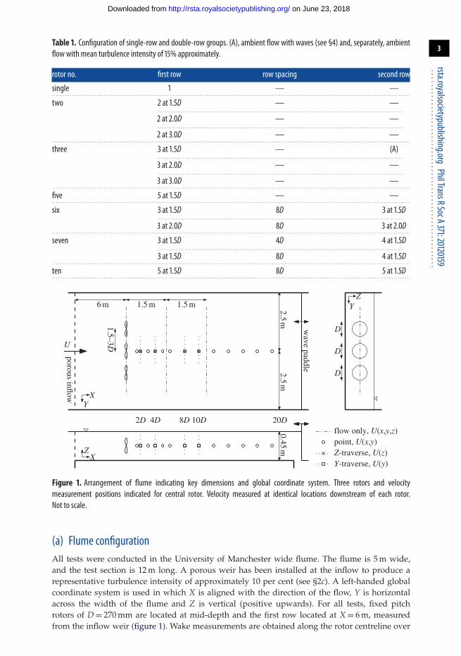
2. Test equipment and procedureThe mean and fluctuating components of velocity have been measured downstream of severalgroups of three-bladed tidal stream turbines. Most measurements were obtained for the samerotor operating point and inflow conditions, such that the effect of lateral spacing on both rotorthrust coefficient and rotor wake can be quantified. The diameter of each rotor is D = 270 mm, thewater depth is 450 mm and the mean velocity is 0.47 cm s−1 (see §2c). At 1:70th geometric scaling,these experiments represent a turbine of diameter 19 m in water depth of 31.5 m and, applyingFroude scaling, a mean incident flow velocity of 3.76 m s−1. The intention of these experiments isto compare the structure of the wake of an isolated rotor with the wake of a rotor located within agroup or array. Experimental measurements have been obtained for up to three rows of devices.The lateral spacing between rotors is in the range 1.5–3D measured centre-to-centre betweenadjacent rotors. The longitudinal spacing between rows is in the range 4–10D, and both staggeredand aligned configurations have been considered. All single- and double-row configurationsstudied are listed in table 1. Measurements from the single-row tests are reported in §3.



3


......................................................

Table 1. Configuration of single-row and double-row groups. (A), ambient flow with waves (see §4) and, separately, ambientflow with mean turbulence intensity of 15% approximately.

rotor no. first row row spacing second row

single 1 — —. . . . . . . . . . . . . . . . . . . . . . . . . . . . . . . . . . . . . . . . . . . . . . . . . . . . . . . . . . . . . . . . . . . . . . . . . . . . . . . . . . . . . . . . . . . . . . . . . . . . . . . . . . . . . . . . . . . . . . . . . . . . . . . . . . . . . . . . . . . . . . . . . . . . . . . . . . . . . . . . . . . . . . . . . . . . . . . . . . . . . . . . . . . . . . . . . . . . . . . . . .

two 2 at 1.5D — —.. . . . . . . . . . . . . . . . . . . . . . . . . . . . . . . . . . . . . . . . . . . . . . . . . . . . . . . . . . . . . . . . . . . . . . . . . . . . . . . . . . . . . . . . . . . . . . . . . . . . . . . . . . . . . . . . . . . . . . . . . . . . . . . . . . . . . . . . . .

2 at 2.0D — —.. . . . . . . . . . . . . . . . . . . . . . . . . . . . . . . . . . . . . . . . . . . . . . . . . . . . . . . . . . . . . . . . . . . . . . . . . . . . . . . . . . . . . . . . . . . . . . . . . . . . . . . . . . . . . . . . . . . . . . . . . . . . . . . . . . . . . . . . . .

2 at 3.0D — —.. . . . . . . . . . . . . . . . . . . . . . . . . . . . . . . . . . . . . . . . . . . . . . . . . . . . . . . . . . . . . . . . . . . . . . . . . . . . . . . . . . . . . . . . . . . . . . . . . . . . . . . . . . . . . . . . . . . . . . . . . . . . . . . . . . . . . . . . . . . . . . . . . . . . . . . . . . . . . . . . . . . . . . . . . . . . . . . . . . . . . . . . . . . . . . . . . . . . . . . . .

three 3 at 1.5D — (A). . . . . . . . . . . . . . . . . . . . . . . . . . . . . . . . . . . . . . . . . . . . . . . . . . . . . . . . . . . . . . . . . . . . . . . . . . . . . . . . . . . . . . . . . . . . . . . . . . . . . . . . . . . . . . . . . . . . . . . . . . . . . . . . . . . . . . . . . . .

3 at 2.0D — —.. . . . . . . . . . . . . . . . . . . . . . . . . . . . . . . . . . . . . . . . . . . . . . . . . . . . . . . . . . . . . . . . . . . . . . . . . . . . . . . . . . . . . . . . . . . . . . . . . . . . . . . . . . . . . . . . . . . . . . . . . . . . . . . . . . . . . . . . . .

3 at 3.0D — —.. . . . . . . . . . . . . . . . . . . . . . . . . . . . . . . . . . . . . . . . . . . . . . . . . . . . . . . . . . . . . . . . . . . . . . . . . . . . . . . . . . . . . . . . . . . . . . . . . . . . . . . . . . . . . . . . . . . . . . . . . . . . . . . . . . . . . . . . . . . . . . . . . . . . . . . . . . . . . . . . . . . . . . . . . . . . . . . . . . . . . . . . . . . . . . . . . . . . . . . . .

five 5 at 1.5D — —.. . . . . . . . . . . . . . . . . . . . . . . . . . . . . . . . . . . . . . . . . . . . . . . . . . . . . . . . . . . . . . . . . . . . . . . . . . . . . . . . . . . . . . . . . . . . . . . . . . . . . . . . . . . . . . . . . . . . . . . . . . . . . . . . . . . . . . . . . . . . . . . . . . . . . . . . . . . . . . . . . . . . . . . . . . . . . . . . . . . . . . . . . . . . . . . . . . . . . . . . .

six 3 at 1.5D 8D 3 at 1.5D. . . . . . . . . . . . . . . . . . . . . . . . . . . . . . . . . . . . . . . . . . . . . . . . . . . . . . . . . . . . . . . . . . . . . . . . . . . . . . . . . . . . . . . . . . . . . . . . . . . . . . . . . . . . . . . . . . . . . . . . . . . . . . . . . . . . . . . . . . .

3 at 2.0D 8D 3 at 2.0D. . . . . . . . . . . . . . . . . . . . . . . . . . . . . . . . . . . . . . . . . . . . . . . . . . . . . . . . . . . . . . . . . . . . . . . . . . . . . . . . . . . . . . . . . . . . . . . . . . . . . . . . . . . . . . . . . . . . . . . . . . . . . . . . . . . . . . . . . . . . . . . . . . . . . . . . . . . . . . . . . . . . . . . . . . . . . . . . . . . . . . . . . . . . . . . . . . . . . . . . . .

seven 3 at 1.5D 4D 4 at 1.5D. . . . . . . . . . . . . . . . . . . . . . . . . . . . . . . . . . . . . . . . . . . . . . . . . . . . . . . . . . . . . . . . . . . . . . . . . . . . . . . . . . . . . . . . . . . . . . . . . . . . . . . . . . . . . . . . . . . . . . . . . . . . . . . . . . . . . . . . . . .

3 at 1.5D 8D 4 at 1.5D. . . . . . . . . . . . . . . . . . . . . . . . . . . . . . . . . . . . . . . . . . . . . . . . . . . . . . . . . . . . . . . . . . . . . . . . . . . . . . . . . . . . . . . . . . . . . . . . . . . . . . . . . . . . . . . . . . . . . . . . . . . . . . . . . . . . . . . . . . . . . . . . . . . . . . . . . . . . . . . . . . . . . . . . . . . . . . . . . . . . . . . . . . . . . . . . . . . . . . . . . .

ten 5 at 1.5D 8D 5 at 1.5D. . . . . . . . . . . . . . . . . . . . . . . . . . . . . . . . . . . . . . . . . . . . . . . . . . . . . . . . . . . . . . . . . . . . . . . . . . . . . . . . . . . . . . . . . . . . . . . . . . . . . . . . . . . . . . . . . . . . . . . . . . . . . . . . . . . . . . . . . . . . . . . . . . . . . . . . . . . . . . . . . . . . . . . . . . . . . . . . . . . . . . . . . . . . . . . . . . . . . . . . . .

U

6 m 1.5 m 1.5 m

XY

Z

ZY

2D 4D 8D 10D

X

20D

0.45 m

D

2.5 m

2.5 m

wave paddle

point, U(x,y)Z-traverse, U(z)Y-traverse, U(y)

flow only, U(x,y,z)

D

D

porous inflow

1.5–3D

Figure 1. Arrangement of flume indicating key dimensions and global coordinate system. Three rotors and velocitymeasurement positions indicated for central rotor. Velocity measured at identical locations downstream of each rotor.Not to scale.

(a) Flume configurationAll tests were conducted in the University of Manchester wide flume. The flume is 5 m wide,and the test section is 12 m long. A porous weir has been installed at the inflow to produce arepresentative turbulence intensity of approximately 10 per cent (see §2c). A left-handed globalcoordinate system is used in which X is aligned with the direction of the flow, Y is horizontalacross the width of the flume and Z is vertical (positive upwards). For all tests, fixed pitchrotors of D = 270 mm are located at mid-depth and the first row located at X = 6 m, measuredfrom the inflow weir (figure 1). Wake measurements are obtained along the rotor centreline over



4


......................................................

the interval 1.5D < x < 20D downstream of the rotor plane, with a detailed study of the wakestructure conducted across vertical cross sections (Y–Z plane) at x = 2D, 4D and ordinates ofinterest up to 12D downstream.

(b) FlowmeasurementTime-varying velocity components (ux, uy, uz) are measured using NORTEK acoustic dopplervelocimeter (ADV) Vectrino+ probes. Mean velocity components (Ux, Uy, Uz), and turbulenceintensities are subsequently obtained. The probes are orientated with their local x-axis alignedwith the global X-axis. The experiments were designed for a mean velocity of approximately0.45 m s−1. For this flow speed, a sampling frequency greater than 32 Hz is required to resolvethe spectral distribution of turbulence into the viscous subrange [9]. Velocity is thus sampled at200 Hz. Analysis of several time histories confirms that 60 s duration is sufficient to determinemean values of velocity and turbulence intensity to within ±2% and cross correlation to within±5%. Each velocity time history, therefore, comprises 12 000 samples. ADV signal quality ismeasured prior to each test, and indicates that the majority of samples (greater than 95%) havea signal-to-noise ratio greater than 15 dB, and a correlation coefficient greater than 75 per cent(definitions as in NORTEK [10]).

(c) Ambient flowTime-varying velocity was recorded at 720 coordinates (40 z-ordinates on each of 18 depthprofiles at different y-ordinates) to understand the spatial variation of the mean flow velocity andturbulence intensity across the test area. The mean longitudinal flow velocity at cross sections ofX = 6, 7.5 and 9 m is U0 = 47 cm s−1 (figure 2). Turbulence intensity is defined relative to meanincident velocity U0 as

TIx =√

(ux − Ux)2

U0. (2.1)

Turbulence intensity is nearly constant across the water depth at each cross section. Averageturbulence intensity is 10 per cent at X = 6 m, but reduces to 8 per cent (approx.) over a distance of3 m (approx. 10D). As a consequence, the rate of momentum recovery may be expected to decreasewith distance downstream. The resultant wake region may be longer than would be observed ifthe incident turbulence intensity were maintained.

Rotors are installed within the central 2 m width of the flume. Over this region, the meanlongitudinal velocity (Ux) varies by less than 3 cm s−1, and the magnitude of longitudinalturbulence intensity (TIx) varies by less than 2 per cent. Outside this region, slightly greatervariation of mean velocity and turbulence intensity is observed. Both Ux and TIx aremarginally lower at the left-hand side of the flow (y < 3.5D) than the right-hand side (y > 3.5D).Approximately 2.5D either side of the centreline of the flume, small regions of reduced flowvelocity are observed and correspond to regions of transverse circulation within the flow. Themean of the transverse components of flow velocity (Uy and Uz) in these regions (not shown)are less than 0.05U0, so are not expected to influence rotor loading or wake recovery. Spanwisevariation of axial velocity (Ux) is minimal, particularly across the area occupied by the rotors(figure 2), and so is neglected to obtain an averaged depth profile and mean mid-depth velocityof U0 = 47 cm s−1 to which wake velocities are normalized.

(d) Rotor and dynamometerAll rotors employed are identical. Each rotor comprises three blades, formed from a Göettingen804 foil with radial variation of chord length and twist angle. This foil section was chosen andthe blade geometry designed such that the variation of thrust coefficient with tip–speed ratio,CT(TSR), is similar to a generic full-scale turbine, despite the moderate chord Reynolds numberof these experiments (Re ≈ 30 000 at 3

4 radius and TSR ∼ 4.5). Details of the rotor design process



5


......................................................

0.950.95

0.95

11

1

1

1

1

1

1.05

1.05

1.051.05

9

9

9

10

10

10

1010

11

11

11

111111

11

0.95

0.95

0.95

0.95

0.95

1

1

11

1

1

1.051.0

1.1

1.

1.05z/

D

–0.5

0

0.5

10

10

1011

11

11

11

11

1111

11

11

11

y/D

z/D

–4 –2 0 2 4y/D

–4 –2 0 2 4

–0.5

0

0.5

(a) (b)

Figure 2. Contours of normalized axial velocity (Ux/U0) and turbulence intensity TIx across Y–Z plane at (a) X = 6 m(corresponding to rotor plane) and (b) 7.5 m (approx. 5D downstream of rotor plane) from inlet, unequal scale.

and predictions of power and thrust coefficients and the measured thrust coefficient curve aregiven by Whelan & Stallard [11]. Rotors are manufactured using a rapid prototyping method toensure that the specified geometry is resolved.

Each rotor is mounted on a 90◦ bevel gear gearbox that is coupled, via a driveshaft, to adynamometer mounted vertically above the waterline. The system was originally developedfor experimental study of arrays of wave energy floats [12,13]. The dynamometer serves twopurposes: (i) at low speeds, an assisting torque is applied to compensate for mechanical frictionin the system and (ii) when rotational speed exceeds a minimum operating speed, a constantretarding torque (τgen) is maintained to represent power extraction. Angular speed (ω) is definedas the rate of change of angular position (φ). Position is measured using an HEDS 9000 quadratureencoder reading an HEDM 6120 T12 code wheel. These codewheels provide 2000 counts perrevolution, and so angular speed is obtained to within 0.1 per cent accuracy when sampled at200 Hz. While speed is greater than a specified minimum (ω > 0.6 rad s−1), the control systemapplies an assisting current IA to produce a constant torque τm = IAkT, where kT is a torqueconstant with a unique value for each motor. For all tests, torque is specified such that the rotoroperates with an average TSR of 4.5 owing to an ambient flow of 0.45 m s−1. Based on blade-element analysis of the three-bladed rotor, an average thrust coefficient of CT = 0.80 is expectedat this operating point [11].

(e) Thrust measurementThe rotor and bevel gearbox are supported on a 15 mm outer-diameter tower that is strain gaugedabove the waterline, and mounted such that the hub height is at mid-depth. The rotor plane islocated 50 mm forward of the centreline of the tower. The moment generated at the top of thesupport structure is measured by a full-bridge strain gauge. Strain gauge voltage is recorded



6


......................................................

via a National Instruments NCC-SG24 module. To calibrate, each tower is mounted horizontally,and fixed increment loads applied to the rotor axis to obtain a linear relationship between loadand measured voltage. Because strain gauges are located above the waterline, the horizontal loadmeasured is due to both horizontal thrust on the swept area of the rotor (Frotor ∼ 1

2 CTρADU20) and

drag distributed over the immersed length of the supporting shaft (Fdrag ∼ 12 CDρBLU2 for a shaft

diameter B = 15 mm and immersed length L = 225 mm). The thrust coefficients reported hereinare based on a rotor force calculated as: Frotor = Ftotal − Ftower. This approach assumes that towerload during operation is similar to the tower load owing to the incident flow alone. Althoughnot exact, this is considered a reasonable approach because, for a mean flow speed of 0.5 m s−1,rotor thrust is an order of magnitude larger than the drag on the supporting shaft (Frotor ∼ 7 N forCT = 1 and ∼ 6 N measured compared with Fdrag ∼ 0.42 N (CD = 1, U = 0.5 m s−1), and less than0.3 N measured).

All time-varying parameters—angular position, applied torque, thrust and flow velocities—are sampled at 200 Hz. Prior to each test, thrust is measured for each rotor in isolation. In alltests reported here, prior to array deployment, TSR = 4.7 ± 0.3 and CT = 0.87 ± 0.05. Thrust andangular speed were measured during each test, such that the modification of thrust owing tolateral blockage and to location within the wake of an upstream turbine can be quantified.Analysis of thrust variation between individual rotors located in the same array and betweendifferent array configurations will be reported in a separate study.

3. Wake structureA summary of the effect of lateral spacing on wake recovery and horizontal and vertical profileis given for the single-row configurations listed in table 1. Downstream of each rotor, threecomponents of velocity are measured at the following locations (see also figure 1):

— along the wake centreline, u(x) at min 12 x-ordinates;— vertical profiles, u(z), at min 2 x-ordinates; and— horizontal profiles, u(y), at min 2 x-ordinates, including x = 2D and 4D.

In the following, the wake velocity deficit is reported based on the measured velocity Ux(z)relative to the ambient flow at the same z-ordinate, U0(z). For lateral traverses, U0 = 0.47 cm s−1

corresponds to the velocity at mid-depth and hub height. Longitudinal turbulence intensity isobtained from equation (2.1). Data files containing the time-averaged velocity components andturbulence intensity for each of the coordinates reported in this study are available as electronicsupplementary material.

(a) Wake recoveryThe measured deficit of mean velocity along the centreline of the wake of a single rotor is foundto be 80 per cent within the near wake of the rotor (1.5D downstream), but recovers to within20 per cent of the incident flow by 10D downstream (figure 3a). Within this distance, normalizedturbulence intensity is between 10 and 15 per cent, with the maximum occurring 3D downstream(figure 3b). Over the range 10–20D, further recovery of mean velocity is gradual, with a deficit of8 per cent observed at 20D. When rotors are located at close lateral spacing, the rate of centrelinevelocity recovery remains similar. However, higher turbulence is observed at 3D downstream(18%) and, further downstream, the wake recovery rate differs between wakes (20–22% at 10Dand 10–17% at 20D). The recovery rate is slightly slower for the central wake.

Porous disc studies at comparable CT [5] report a similar velocity deficit at 20D, but therate of decay is different, 40 per cent at 4D and 15 per cent at 10D. Porous disc tests at higherblockage ratios based on swept area [6] observe recovery over a shorter distance (10% deficit 10Ddownstream). A deficit of 22 per cent has been measured 10D downstream of a three-bladed rotoroperating at a slightly lower thrust coefficient (CT = 0.77) [5]. However, the deficit is larger closer



7


......................................................

0 5 10 15 20

x/D

0 5 10 15 20

x/D

0.2

0.4

0.6

0.8

1.0

5

10

15

20

TI x

1 –

Ux/

U0

(a) (b)

Figure 3. Longitudinal variation of (a) velocity deficit and (b) turbulence intensity downstream of isolated rotor (filled circles),and three rotors at 1.5D lateral spacing: centre rotor (thick curve), and rotors at+1.5D (thin curve) and−1.5D (dashed curve).

to the turbine (43% deficit at 6D). For a rotor with a similar predicted thrust variation with TSR tothe rotors used here (TSR = 5, CT not specified) [4], the near-wake deficit was found to be lower(53% at 2D), but a similar recovery is observed further downstream (35% at 6D and 15% at 10D).In part, these differences could be attributed to the presence of a tower wake [3], but, becausethe tower has a small diameter and is close to the rotor plane, this wake is expected to be smallrelative to the rotor wake. Differences may also be due to the proximity of bounding surfaces;here, the depth is 1.67D compared with more than 2.5D in the single rotor studies.

(b) Lateral expansionA section across the wake of a single rotor at mid-depth (Ux(y), figure 4a) indicates that the lateralwake profile approaches a symmetric, approximately Gaussian, distribution at both 2D and 4Ddownstream. Consistent with figure 3, the maximum velocity deficits at the centreline of the wakeare 80 per cent and 50 per cent at 2D and 4D downstream, respectively. Over the same distance,the wake width expands from approximately 1.5 to 2D. Wakes from adjacent turbines at 1.5Dspacing would, therefore, be expected to interact after 2D downstream. This is observed for tworotors at 1.5D spacing (figure 4b), for which the velocity deficit mid-distance between wakes isapproximately 10 per cent, and turbulence intensity between the rotor centrelines is higher thanoutside of the rotor centrelines. This is due to overlap of the shear layers from adjacent wakes.

The profile of each wake behind two rotors remains similar to that of an isolated rotor, butboth wakes are slightly asymmetric. Maximum velocity deficit occurs at 0.1D outwards from thecentreline of the rotor at y = +1.5D. Similar asymmetry is observed for the two outermost wakesdownstream of a row of three rotors for which the maximum velocity deficit is observed 0.2Doutwards from the centreline of the rotor (figure 4c). This is due to a lower velocity deficit in theregion between wakes (i.e. 0.75 < |y/D| < 1.5) rather than a shift of the isolated wake profile. Onthe unconstrained side of the wake (|y| > 1.5D), the profile of velocity deficit is similar to that ofan isolated rotor.

The wake of a centre turbine in a row of three represents a wake constrained by symmetricboundary conditions. This wake is narrower than either the outermost wakes or the wake of anisolated rotor. This can be attributed to a higher rate of velocity recovery owing to the elevatedturbulence intensity in the region between rotor centrelines. By 4D downstream, the maximumvelocity deficit near the centre of an isolated wake reduces to 45 per cent. The maximum deficit isa little lower, approximately 42 per cent, for both two rotors and three rotors. At this distance, thedeficit between rotors is nearly 30 per cent, and turbulence intensity is higher in the shear layersbetween rotors than the outermost shear layers. The wake profile approaches that of an isolatedrotor, as the separation between three rotors is increased (figure 4d). For 3D lateral spacing, each



8


......................................................

0 0.2 0.4 0.6 0.8–1.5

–1.0

–0.5

0

0.5

1.0

1.5

y/D

y/D

0 10 20 30

TIx

–1.5

–1.0

–0.5

0

0.5

1.0

1.5

2.0

2.5

3.0

–3

–2

–1

0

1

2

3

0.5

1.0

1.5

2.0

2.5

3.0

3.5

4.0

4.5

1 – Ux/U0

0 0.2 0.4 0.6 0.8 0 10 20 30TIx1 – Ux/U0

0 0.2 0.4 0.6 0.81–Ux/U0

0 0.2 0.4 0.6 0.81 – Ux/U0

0 0.2 0.4 0.6 0.8 0 10 20 30

TIx1 – Ux/U0

(a)

(b)

(c)

(d)

Figure 4. (a–d) Lateral profiles of velocity deficit and turbulence intensity at mid-depth downstream of a single rotor, tworotors and three rotors at 1.5D lateral spacing. Profiles at x = 2D (thick curve) and 4D (thin curve). Profile of isolated rotor wake(a) also shown (filled circles) in (b)–(d).

wake is very similar to the isolated wake of figure 4a. For 2D lateral spacing, the ambient flow isunchanged between the rotors by 2D downstream, although asymmetry of the outermost wakeis observed and, by 4D downstream, the wakes begin to merge.

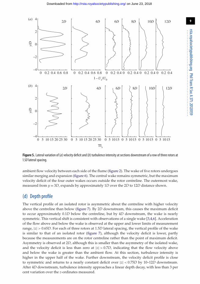
(c) Wake mergingFurther downstream of the array of three rotors at 1.5D lateral spacing (figure 5), the wakesfrom individual rotors merge to form a single wake. At 6D downstream, individual wakesare still identifiable, but by 8D downstream, there is little variation of velocity deficit acrossthe width between centres of the outermost rotors (|y| < 1.5D). Beyond 8D downstream, thevelocity deficit is nearly constant over the width of the wakes (velocity deficit approx. 23% over|y| < 1.75D at 8D downstream). Turbulence intensity is also constant over the width of the wakeby 8D downstream and only 1–2% greater than the ambient turbulence. Further downstream,velocity recovers to within 20 per cent of the ambient flow by 10–12D.

Over the 10D length of the wake shown, the outermost wake expands from 1D to 2D of therotor centreline at y = 1.5D. For example, zero deficit occurs at y = 2.5D at x = 2D, but at y > 3.5Dat x = 12D. Note that in the three-rotor study of figure 5b, the turbulence intensity is higherand the velocity deficit lower on one side of the flow (y > +3D) than the other (y < −3D). Thisdiscrepancy is not due to the wakes, but occurs due to the small difference, less than 2 cm s−1, of



9


......................................................

–4

–2

0

2

4

y/D

0 5 10 15 20 25 30

2D 4D

0 5 1015

6D 8D 10D 12D

TIx

1 – Ux/U0

0 0.2 0.4 0.6 0.8–4

4

0 0.2 0.4

–2

0

2y/

D

2D 4D 6D 8D 10D 12D

0 0.2 0.4 0.6 0.8 0 0.2 0.4 0 0.2 0.4 0 0.2 0.4

0 5 10 15 20 25 30 0 5 1015 0 5 1015 5 10150

(a)

(b)

Figure 5. Lateral variation of (a) velocity deficit and (b) turbulence intensity at sections downstream of a row of three rotors at1.5D lateral spacing.

ambient flow velocity between each side of the flume (figure 2). The wake of five rotors undergoessimilar merging and expansion (figure 6). The central wake remains symmetric, but the maximumvelocity deficit of the four outer wakes occurs outside the rotor centreline. The outermost wake,measured from y = 3D, expands by approximately 1D over the 2D to 12D distance shown.

(d) Depth profileThe vertical profile of an isolated rotor is asymmetric about the centreline with higher velocityabove the centreline than below (figure 7). By 2D downstream, this causes the maximum deficitto occur approximately 0.1D below the centreline, but by 4D downstream, the wake is nearlysymmetric. This vertical shift is consistent with observations of a single wake [3,4,6]. Accelerationof the flow above and below the wake is observed at the upper and lower limits of measurementrange, |z| > 0.65D. For each of three rotors at 1.5D lateral spacing, the vertical profile of the wakeis similar to that of an isolated rotor (figure 7), although the velocity deficit is lower, partlybecause the measurements are on the rotor centreline rather than the point of maximum deficit.Asymmetry is observed at 2D, although this is smaller than the asymmetry of the isolated wake,and the velocity deficit is less than zero at |z| > 0.7D, indicating that the flow velocity aboveand below the wake is greater than the ambient flow. At this section, turbulence intensity ishigher in the upper half of the wake. Further downstream, the velocity deficit profile is closeto symmetric and returns to a nearly constant deficit over |z| < 0.75D by 10–12D downstream.After 4D downstream, turbulence intensity approaches a linear depth decay, with less than 3 percent variation over the z-ordinates measured.



10


......................................................

0 0.2 0.4 0.6 0.8–5

–4

–3

–2

–1

0

1

2

3

4

5

y/D

2D

0 0.2 0.4 0.6 0.8

4D

0 0.2 0.4

8D

0 0.2 0.4

10D

0 0.2 0.4

12D

1 – Ux/U0

Figure 6. Lateral variation of velocity deficit at five sections downstream of a row of five rotors at 1.5D lateral spacing.

1 − Ux(z)/U0(z)

0 5 10 15 20 25 30

–0.5

0

0.5

2D 4D

0 5 1015TIx

6D

00 5 1015

8D

000 5 1015

10D 12D

0 0.2 0.4 0.6 0.8

–0.5

0

0.5

z/D

z/D

2D 4D

0 0.2 0.4

6D 8D 10D 12D

0 0.2 0.4 0.6 0.8 0 0.2 0.4 0 0.2 0.4 0 0.2 0.4

0 5 10 15 20 25 30 000 5 1015

(a)

(b)

Figure 7. Depth profiles of (a) velocity deficit and (b) turbulence intensity downstream of three rotors at 1.5D lateral spacing:centre rotor (thick solid curve) and rotors at+1.5D (solid curve) and−1.5D (dashed curve). Profile of single rotor also shown(filled circles) at x = 2D.



11


......................................................

0 2 4 6 8 10 12

0.2

0.4

0.6

0.8

1.0

x/D0 2 4 6 8 10 12

x/D

1 –

Ux/

U0

5

10

15

20

TI x

(a) (b)

Figure 8. As figure 3 with opposing waves on ambient flow.

0 0.2 0.4 0.6 0.8–3

–2

–1

0

1

2

3

1 − Ux/U0

y/D

0 10 20 30TIx TIx

–1

–0.5

0

0.5

1

1 − Ux(z)/U0(z)

z/D

0 0.2 0.4 0.6 0.8 0 10 20 30

(a)

(b)

Figure 9. (a,b) Profiles of wake of three rotors owing to incident flow and opposing waves. Single rotor also shown for x = 2D(filled circles).

4. Ambient flow and wavesThe foregoing wake studies are due to the incident flow detailed in §2c. Although theseconditions are expected to be reasonably representative, flow fluctuations owing to both wavesand large-scale turbulence occur at tidal stream sites [14], and are expected to affect wakerecovery [15].

The modification of rotor wakes owing to an irregular wave field with a measured peakfrequency of 0.8 Hz (1.25 s) and a measured significant wave height of 50 mm has been studied.Applying Froude scaling, these conditions are equivalent to a peak period of approximately 10.5 sand a significant wave height of 3.5 m in water depth of 31.5 m. These waves have longer periodsthan conditions observed at the European Marine Energy Centre tidal site [16], but are selectedsuch that fluctuations are imposed over the water depth. Turbulent fluctuations can be separatedfrom lower frequency wave-induced kinematics, but here turbulence intensity describes allfluctuations about the mean. Close to the surface, turbulence intensity is approximately 25 percent, but this decays to a similar profile to the ambient flow below mid-depth.

The mean thrust on each rotor is similar without and with waves. However, rotor loadingvaries considerably (±25% approx.) owing to oscillation of the incident flow. Velocity deficitimmediately downstream of the rotors is lower than for the wake of an isolated rotor, but the



12


......................................................

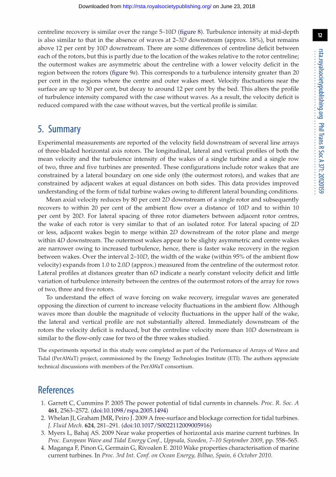
centreline recovery is similar over the range 5–10D (figure 8). Turbulence intensity at mid-depthis also similar to that in the absence of waves at 2–3D downstream (approx. 18%), but remainsabove 12 per cent by 10D downstream. There are some differences of centreline deficit betweeneach of the rotors, but this is partly due to the location of the wakes relative to the rotor centreline;the outermost wakes are asymmetric about the centreline with a lower velocity deficit in theregion between the rotors (figure 9a). This corresponds to a turbulence intensity greater than 20per cent in the regions where the centre and outer wakes meet. Velocity fluctuations near thesurface are up to 30 per cent, but decay to around 12 per cent by the bed. This alters the profileof turbulence intensity compared with the case without waves. As a result, the velocity deficit isreduced compared with the case without waves, but the vertical profile is similar.

5. SummaryExperimental measurements are reported of the velocity field downstream of several line arraysof three-bladed horizontal axis rotors. The longitudinal, lateral and vertical profiles of both themean velocity and the turbulence intensity of the wakes of a single turbine and a single rowof two, three and five turbines are presented. These configurations include rotor wakes that areconstrained by a lateral boundary on one side only (the outermost rotors), and wakes that areconstrained by adjacent wakes at equal distances on both sides. This data provides improvedunderstanding of the form of tidal turbine wakes owing to different lateral bounding conditions.

Mean axial velocity reduces by 80 per cent 2D downstream of a single rotor and subsequentlyrecovers to within 20 per cent of the ambient flow over a distance of 10D and to within 10per cent by 20D. For lateral spacing of three rotor diameters between adjacent rotor centres,the wake of each rotor is very similar to that of an isolated rotor. For lateral spacing of 2Dor less, adjacent wakes begin to merge within 2D downstream of the rotor plane and mergewithin 4D downstream. The outermost wakes appear to be slighty asymmetric and centre wakesare narrower owing to increased turbulence, hence, there is faster wake recovery in the regionbetween wakes. Over the interval 2–10D, the width of the wake (within 95% of the ambient flowvelocity) expands from 1.0 to 2.0D (approx.) measured from the centreline of the outermost rotor.Lateral profiles at distances greater than 6D indicate a nearly constant velocity deficit and littlevariation of turbulence intensity between the centres of the outermost rotors of the array for rowsof two, three and five rotors.

To understand the effect of wave forcing on wake recovery, irregular waves are generatedopposing the direction of current to increase velocity fluctuations in the ambient flow. Althoughwaves more than double the magnitude of velocity fluctuations in the upper half of the wake,the lateral and vertical profile are not substantially altered. Immediately downstream of therotors the velocity deficit is reduced, but the centreline velocity more than 10D downstream issimilar to the flow-only case for two of the three wakes studied.

The experiments reported in this study were completed as part of the Performance of Arrays of Wave andTidal (PerAWaT) project, commissioned by the Energy Technologies Institute (ETI). The authors appreciatetechnical discussions with members of the PerAWaT consortium.

References1. Garrett C, Cummins P. 2005 The power potential of tidal currents in channels. Proc. R. Soc. A

461, 2563–2572. (doi:10.1098/rspa.2005.1494)2. Whelan JI, Graham JMR, Peiro J. 2009 A free-surface and blockage correction for tidal turbines.

J. Fluid Mech. 624, 281–291. (doi:10.1017/S0022112009005916)3. Myers L, Bahaj AS. 2009 Near wake properties of horizontal axis marine current turbines. In

Proc. European Wave and Tidal Energy Conf., Uppsala, Sweden, 7–10 September 2009, pp. 558–565.4. Maganga F, Pinon G, Germain G, Rivoalen E. 2010 Wake properties characterisation of marine

current turbines. In Proc. 3rd Int. Conf. on Ocean Energy, Bilbao, Spain, 6 October 2010.


http://dx.doi.org/doi:10.1098/rspa.2005.1494

http://dx.doi.org/doi:10.1017/S0022112009005916


13


......................................................

5. Bahaj AS, Myers LE, Thomson MD, Jorge N. 2007 Characterising the wake of horizontal axismarine current turbines. In Proc. 7th European Wave and Tidal Energy Conf., Porto, Portugal,11–13 September 2007.

6. Sun X, Chick JP, Bryden IG. 2007 Laboratory-scale simulation of energy extraction from tidalcurrents. Renew. Energy 33, 1267–1274. (doi:10.1016/j.renene.2007.06.018)

7. Hassan U. 1993 A wind tunnel investigation of the wake structure within small wind turbinefarms. Technical Report ETSU WN 5113, Garrad Hassan and Partners Ltd, Bristol, UK.

8. Myers LE, Bahaj AS. 2012 An experimental investigation simulating flow effects in firstgeneration marine current energy converter arrays. Renew. Energy 37, 28–36. (doi:10.1016/j.renene.2011.03.043)

9. Nezu I, Nakagawa H. 1993 Turbulence in open-channel flows. Rotterdam, The Netherlands:IAHR/AIRH, A. A. Balkema.

10. NORTEK. 2004 Vectrino velocimeter user guide. Norway: NORTEK AS.11. Whelan JI, Stallard TJ. 2011 Arguments for modifying the geometry of a scale model rotor. In

Proc. European Wave and Tidal Energy Conf., Southampton, UK, 5–9 September 2011.12. Brown RJ. 2009 Design and construction of a dynamometer system for testing an array of

wave energy point absorbers. MPhil Thesis, University of Manchester, Manchester, UK.13. Weller SD, Stallard TJ, Stansby PK. 2010 Experimental measurements of irregular wave

interaction factors in closely spaced arrays. IET Renew. Power Generat. 4, 628–637. (doi:10.1049/iet-rpg.2009.0192)

14. Norris JV, Droniou E. 2007 Update on EMEC activities, resource description, andcharacterisation of wave-induced velocities in a tidal flow. In Proc. 7th European Wave andTidal Energy Conf., Porto, Portugal, 11–13 September 2007.

15. Gant SE, Stallard TJ. 2008 Unsteady loading of tidal stream turbines. In Proc. 18th Int. Offshoreand Polar Engineering Conf., Vancover, BC, 6–11 July 2008.

16. Thomson M, McCann G, Hitchcock S. 2008 Implications of site-specific conditions on theprediction of loading and power performance of a tidal stream device. In Proc. 2nd Int. Conf.on Ocean Energy, Brest, France, 15–17 October 2008.


http://dx.doi.org/doi:10.1016/j.renene.2007.06.018



http://dx.doi.org/doi:10.1049/iet-rpg.2009.0192

http://dx.doi.org/doi:10.1049/iet-rpg.2009.0192


interactionsbetweentidal turbinewakes:experimental...

Documents