interactions in polymer blends-relationship between thermodynamic and scattering measurements

Interactions in Polymer Blends-Relationship Between Thermodynamic and Scattering Measurements

J. S. HIGGINS and D. J. WALSH

Department of Chemical Engineering and Chemical Technology Zmperial College

Prince Consort Road London SW7 2BY England

Methods of preparation and of determining miscibility limits for partially miscible binary polymer blends are described. An equation-of-state, theoretical description of this behavior is introduced and the terms describing interactions within the system discussed. Values of these interaction terms are obtained by fitting the models to measured cloud point curves, heats of mixing data, etc. The use of neutron scattering experiments to obtain molecular conformation and interaction parameters is described and a comparison made with values extracted from the thermodynamic measurements.

INTRODUCTION ecause of their low combinatorial entropy of B mixing, polymers are expected to be immisci-

ble with each other. Miscibility of polymers occurs in three situations:

1) polymers of low molecular weight which no longer have a negligible entropy of mixing (1, 2);

2) polymers which are chemically very similar and have a very small unfavorable heat of mixing

3) polymers which show specific interactions between the molecules resulting in favorable heats of mixing (5-8).

The combinatorial entropy of mixing is usually assumed to have the form given in the classical Flory-Huggins equation.

( 3 , 4);

AS = -k(N1 In r#q + Nzln 4 2 ) (1)

Further contributions to the free energy of mixing arise from volume changes on mixing which were assumed to be zero in the Flory-Huggins theory. Remaining contributions to the free energy come in terms, the sign and magnitude of which are governed by an interaction parameter, x, in the Flory Huggins theory or Xlz in the Equation-of- State theory of Flory and his co-workers (9, 10). These interaction parameters can be related by

The symbols used in this and other equations are given in the Symbols List.

In some treatments an additional contribution from a non-combinatorial entropy of mixing is con-

sidered, the sign and magnitude of which is governed by the parameter Q l Z . In other cases this contribution is included within the definition of Xl2

or assumed to be zero. For convenience and to avoid confusion we will therefore use (1 1)

X I 2 = X I 2 - TtjQ12 (3) In this paper we will discuss the different meth-

ods used to obtain experimental values of the interaction parameter, some of which yield Xlz and some X12. In particular we will discuss the relationship between data obtained using scattering methods with other methods.

Systems which show partial miscibility at some temperatures are advantageous for study because the measurement of a phase diagram provides another measure of the interaction parameter, or more normally a way of checking the experimental interaction parameters by using them to simulate the phase diagram (7, 12, 13). We will therefore start with a short description of the ways we have used to prepare mixtures, establish miscibility, and measure phase diagrams.

Observation of Miscibility and Phase Diagrams

Mixtures can be prepared by three methods: mechanical mixing, mixing in a common solvent fol- lowed by evaporation or precipitation, and in situ polymerization.

In the case of low molecular weight polymers, mechanical mixing can easily be achieved but in the case of most of the high molecular weight polymers which we have investigated this has not been possible due to their poor thermal stability for ex- tended periods at high temperatures.

Solvent casting is the commonest method of pre-

POLYMER EUGIiUEERlNG AND SCIENCE, MIWUNE, 1984, Vol. 24, No. 8 555

J. S. Higgins and D. J. Walsh

t a d

1 s -

paring homogeneous mixtures and we have used it extensively ( 5 , 7, 8, 14). Mixing in a common solvent does not however guarantee a homogeneous blend even for miscible polymers. Regions of two phase coexistence within the polymer/polymer/solvent three component phase diagram can cause phase separated structures to be formed. For example, with poly(viny1 chloride)/poly(ethyl acrylate), no suitable solvents have yet been found to produce homogeneous blends and mixtures can only be prepared by in situ polymerization ( 1 5 ) .

In situ polymerization is the polymerization of one monomer in the presence of another polymer and has many advantages in the preparation of blends. It does not, however, guarantee that homogeneous blends can be prepared at all compositions. In the preparation of poly(viny1 chloride) (PVC)/solution chlorinated polyethylene blends, vinyl chloride is only partially miscible with chlorinated polyethylene ( 3 ) , which limits the range of compositions prepared by a one-step polymerization. In the preparation of PVC/poly(butyl acrylate) blends, vinyl chloride is completely miscible with poly(buty1 acrylate) but a two phase region exists within the polymer/polymer/monomer three component phase diagram as shown in Fig. 1 (16). Polymerization from A to B produces a homogeneous blend whereas from E to H produces a two phase structure. The polymerization pathway en- ters a two phase region at F and when leaving at G the mixture does not become homogeneous. It is possible to reswell composition B to C and repo- lymerize to D to produce a homogeneous blend. When phase separation takes place it appears to produce a mixture of relatively pure PVC plus a blend of approximately 50/50 composition. The tie lines are believed to radiate from the apex as shown.

We have established the miscibility of blends by

PVC D H B Fig. 1 . The three component phase diagram for oinyl chloride/ poly(buty1 acrylate)/poly(oinyl chloride). The lines within the diagram represent polymerization pathways.

optical clarity which is especially useful and more reliable in the case of low molecular weight mixtures (1, 2). For high molecular weight blends we have used a variety of techniques including microscopy, electron microscopy, differential scanning calorimetry (D.S.C.), differential thermal analysis (D.T.A.), dielectric relaxation, and dynamic mechanical analysis. Dynamic mechanical analysis is considered to be the single most useful technique. Figure 2 shows an example of the single, composition dependent glass transition peaks obtained for blends of poly(buty1 acrylate) with chlorinated polyethylene (7). In general, not all techniques are suitable for any given blend and all can produce misleading evidence in some circumstances. We therefore prefer to use two or more techniques giving corroborating evidence in order to establish miscibility.

Phase diagrams can be obtained by turbidity- temperature measurements but this is only suitable for high molecular weight polymers if they have sufficient mobility. In the case of blends of chlorinated polyethylene with ethylene-vinyl acetate copolymer very reproducible plots of this kind can be obtained as shown in Fig. 3 , and we have been able to obtain the cloud point curves as shown in Fig. 4 (17). Other methods include dynamic mechanical analysis of heated and quenched samples (3 , 16), microscopy, and electron microscopy (16, 17). In general, we would again prefer to see corroborating evidence for the miscibility limits from two or more techniques.

Non-Scattering Methods for Studying Interactions

The most direct way of studying the interactions between two polymers is by measuring the heats of mixing (AHm). These can be related to the interaction energy parameter Xlz by

AH,,, = FiV2j"[r$lPlo(i;l-' - 6-l) (4) + &Pz"(i;z-' - c-1) + r$&X12/d]

L I I I 50 100 ac

Fig 2. Plots of tan 6 against temperuture for blends of chlori- nutetf polyethylene with poly(buty1 acrylate) showing single corn- position dependent glass transition temperatures.

556 POLYMER ENGINEERING AND SCIENCE, MID-JUNE, 1984, Vol. 24, No. 8


-0.05

-1.00

-1.50

"r

-

-

-

0 Temperature ( C)

Fig. 3. Plot of scattering intensity (arbitrary units) against temperature for a blend of chlorinated polyethylene with an ethylene- vinyl acetate copolymer.

20 40 60 80

% CPE Fig 4 Phase diagrams for chlorinated polyethylene with ethylene-vinyl acetate copolymers having 40 and 45 percent (upper curve) vinyl acetate

Measurements can be made directly in the case of oligomer mixtures by mixing the two materials in a calorimeter. Figure 5 shows the heats of mixing measured for mixtures of oligomeric poly(ethy1ene

oxide) and poly(propy1ene oxide) (1). These are positive (unfavorable) and predict a positive interaction parameter.

With high molecular weight polymers, direct mixing is not possible and measurements must be made on oligomers or low' molecular weight analogues. This is not completely satisfactory because there may be molecular weight dependencies due to end group or density effects. Figure 6 shows the heats of mixing of mixtures of a chlorinated hydro- carbon with 2-ethyl hexyl acetate (8) which are used as analogues for chlorinated polyethylene and ethylene-vinyl acetate copolymer. The heats of mixing are negative (favorable) and predict a negative interaction parameter.

The interaction parameter can also be obtained from inverse gas chromatography (I.G.C.). In this case X , z is obtained. The polymers are coated onto an inert support which is packed into the column of a gas chromatograph. Various solvent probes are injected into the column and the retention volumes measured. Measurements on the two base polymers and the blend must be used to calculate XI, .

I.G.C. has been used to calculate interaction parameters for a series of polyacrylates and polymeth- acrylates with PVC (18). The exact values obtained

Fig. 5. Heats of mixing of a poly(ethy1ene glycol) dimethyl ether, with a poly(propy1ene glycol) dimethyl ether at 50°C. PEG mol. wt = 600, PPG mol. wt = 0, 1,000; 0, 1,500; 8, 2,000.

0.0 0.2 0.4 0.6 0.8 d

-2.m [

S52

Fig. 6 Heats of mixing of sec. octyl acetate with a chlorinated paraffin plotted against weight fraction of clilorinated paraffin (S52) at X 64.5, 0 73.08,. 83.5"C.

POLYMER ENGINEERING AND SCIENCE, MIDJUNE, 1984, Vol. 24, No. 8 557


should not be given too much weight. They can only be obtained at temperatures well above the Tg's of the polymers. They also are liable to error due to non-equilibrium absorption and surface ad- sorption as discussed elsewhere (19). The accumu- lated errors from measurements on the individual polymers and the blend can add to a large error in the result. If phase separation occurs in the blend the solvent retention measured is a mean of the two polymers, and a correct value of XI2 will not be obtained (20).

Simulation of Phase Boundaries

tions given by The spinodal is the limit of metastable composi-

d(Api/RT)/d& I T,P = 0

The origins of the phase diagram have been discussed in many books and reviews (21) and will not be discussed here. The form of the spinodal equation which we have used is (7, 12, 13):

- l /h + (1 - r 1 / d - (P1"V1"/RTI')(d6/d~2)/[v2'3(61'3 - l)]

( 5 ) + (PI"V1"/RT)(c-~ + &)dv/d@a

+ (VlUX12/RT) x

x [(281022/6$1&) - (02"62)dv/a42]

- (vl"91a/R)(281822/~1~2) = 0 The first two terms in this equation are the com-

birratorial entropy terms, the third and fourth are the equation-of-state terms, the fifth represents the interaction energy term, and the sixth the non- combinatorial entropy term.

The procedure used in simulating a spinodal equation is to use a value of X 1 2 derived from heat of mixing measurements and to adjust the value of Q 1 2 to fit the equation to the minimum in the experimental cloud point curve. The total spinodal curve can then be calculated and compared with the experimental cloud point curve. The cloud point curve should lie between the binodal and the spinodal or lie on the spinodal if the method of phase separation is spinodal decomposition. The calculated spinodal should therefore be on or just inside the cloud point curve. Figure 7 shows the observed cloud point curves

and simulated spinodals for mixtures of chlorinated octadecane and oligomeric poly(methy1 methacrylate) which show UCST behavior (12). In this case the cloud point for low molecular weight materials might be expected to more nearly match the binodal and it is not surprising that the spinodal is much more curved. Figure 8 shows the observed cloud point curves

and simulated spinodal for chlorinated polyethylene/poly(butyl acrylate) mixtures (7). The simu-

1501

O t I r I A+- I \ - 5 0 t

Weight fraction COD Fig. 7. Phase diagram from oligomeric mixtures of poly(methy1 methacrylate) (Mn = 434) with chlorinated octadecanes w t percent chlorine A 17.4, B 24.6, C 33.4. Solid lines experimental data, broken lines calculated spinodal.

SIMULATION OF SPINODAL PBA/CPE 12

Temp.

(K)

350

Fig. 8. Simulated spinodals for blends of poly(buty1 acrylate) with chlorinated polyethylene using (1 ) Xl2 = -94 (atm) (from experimental AH), Q12 = -0.235 (atm/K); (2) XIZ = -30, Q12 =

-0.0034. The dotted line follows the experimental cloud point curve.

-0.076; (3) XI* = -10, Ql2 = -0.026; (4) Xi2 = -1 , Qlz =

lated spinodal is flat-bottomed and lies outside the cloud point curve which is an impossible situation. A much lower value of X 1 2 (and hence also Q 1 2 )

558 POLYMER ENGINEERING AND SCIENCE, MIDJUNE, 1984, V d . 24, No. 8


must be used to fit the experimental results. We believe that this is due to the temperature dependence of Xlz or to differences between the polymers and the oligomers used to find AHm. In all cases where a favorable AHm gives a favorable XIZ we have found it necessary to include an unfavorable Qlz to fit the theory with the experimental results.

Scattering from Two Component Systems

Concentration fluctuations in a liquid mixture which give rise to scattering of radiation are them- selves related to the gradient of the chemical potential with respect to composition (22-24). Obser- vation of scattered intensity at the forward angle, I (o ) can then give information on the interaction parameter directly.

(6) K R T v I ~ z

W P l ) / a 4 z Z(0) =

where K takes account of experimental geometry and scattering cross sections.

At the spinodal temperature (where a(Apl) / a4z = 0) it is predicted that the turbidity will tend to infinity. It is clear from E q 6 that scattering measurements will yield an interaction parameter containing all contributions (enthalpic and entropic) to the free energy of mixing, i.e. in relating the x obtained to X l z via Eq 2 one would in fact obtain XI, defined as in Eq 3.

In neutron scattering experiments deuterium la- beling can be applied in order to obtain information concerning the molecular conformation as well as the interactions. Recent papers (2.5-27) have examined in detail the neutron scattering from blend systems and shown how to separate the molecular conformation and interaction terms. If we ignore for the moment any effect of deuteration on the thermodynamics of the system then the angular variation of scattering from a blend of polymer 1 + its deuterated analog + polymer 2 is (25):

(cd + (1 - c)h - b f ) 2 '(') = xl-'(Q) + p2x,-'(Q) - 2pp

(7) + ~ ( 1 - c)(d - h)'~i(Q)

where Q = (4II/h) sin - and 6' is the scattering

angle; c is the fraction of polymer 1 segments deuterated. d and h are the net neutron scattering lengths (28) for deuterated and hydrogenous segments of polymer 1, b' = pb and b is the scattering length per segment of polymer 2. p = vI/vz where 01, v2 are segment specific volumes for polymers 1 and 2 respectively

( 3

x n ( Q ) = 4nNnMQRg") (8) +,, is the segment concentration, N,, the degree of polymerization and Rg" the radius of gyration of polymer species n. In more familiar terms the vol-

ume fraction 4"' = 4nmn/pnNA.mn is the segment mass and pn the density of polymer species n. fD(QRg") is the Debye scattering curve for ideal polymers which at low Q can be approximated to:

U is the Flory interaction parameter here expressed per segment volume. In terms of the conventional Flory x per lattice point

The first of the terms in Eq 7 arises from concentration fluctuations the second gives the conformation of the labeled molecules. The form of the concentration fluctuation term is based on the Flory-Hug- gins lattice theory; the denominator is effectively

d(Apl)/d& calculated from that model. If 1 RTvi4z comparison with other models is to be made then the relevant calculation of this term must be substi- tuted in Eq 7. It appears generally simpler at this stage to extract a Flory x, knowing it may be a complex function of temperature and concentration.

There are a number of ways of manipulating Eq 7 by varying c and $1 in order to obtain Rg" and U from the observed scattering S(Q), and these will be outlined here.

Method 1

If c = 1 and 41 + 0 we regain the simple Zimm formula (24, 28) for scattering from dilute solution

pz/Nzm2 = molar volume of polymer 2. Thus a conventional Zimm analysis will yield Rg' and U but only at very small 4,.

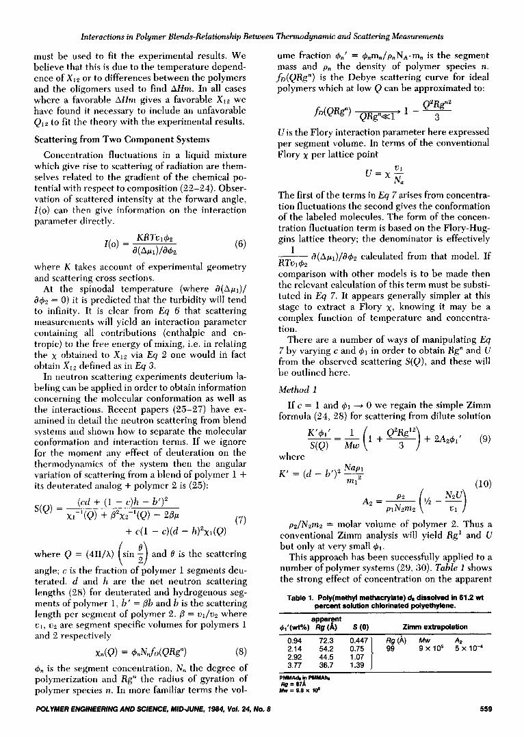
This approach has been successfully applied to a number of polymer systems (29, 30). TubZe 1 shows the strong effect of concentration on the apparent

Table 1. Poly(methy1 methacrylate) de dissolved in 61.2 wt percent solution chlorinated polyethylene.

0.94 72.3 0.447 Rg (A) Mw A2 2.14 y:;; } 99 9x105 5x1O4 2.92 3.77 36.7 1.39

PMMld. in PMMAh. Rg = 8?A Mw = 9.8 x 16

POLYMER ENGINEERING AND SCIENCE, MID-JUNE, 1984, Vol. 24, No. 8 559

1. S . Higgins and 0.1. Walsh

radius of gyration (obtained using Eq 9 but ignoring the A2 term) and the intensity at Q = 0 for a blend of polymethyl methacrylate (I) with solution chlorinated polyethylene (31). At this level of chlorination the polymers are perfectly compatible and the SCPE forms a good solvent for the PMMA as con- firmed by the expanded radius of gyration (obtained by extrapolation to = 0) as compared to its value in the homopolymer, and a positive Az. Analysis of A2 i n terms of E q 10 then yields a large negative value of x (or U ) as expected for a compatible pair, arid the behavior can be examined as a function of temperature.

Information from other measurements indicated that x may depend on concentration as well as temperature. In this case a different method of exploiting Eq 7 must be used.

Method 2

ent values of c and a weighted subtraction Measurements at a finite (fixed) $1 for two differ-

will yield

[.I(] - c1) - cz(l - C z ) l ( d - h)2XI(Q) (12) and hence Rg'. It is essential to remove correctly all background scattering and especially the iso- tropic incoherent scattering from the sample which may be substantial. This cannot be measured con- ventionally by using a purely hydrogenous sample since even at c = 0 the fluctuation term in Ey 7 is non zero. Nor can it be calculated from the com- piled bound atom cross sections (o , , ,~ = 81 X cm2 for hydrogen) since as we have observed (32 ) u,,,, is always greater than the quoted value and moreover increases with increasing molecular mobility. (For example, the effective hydrogen cross section in polystyrene increases from 125 x cm2 at around T,: to over 160 x 1 0-24 cm' at around 2 60 O C.)

If the molecular mobility is altered in the blends, constructing an incoherent background from that measured for the two polymers separately may also prove difficult. For these reasons we have preferred yet another approach to E q 5, although Method 2 has been applied by other workers apparently rea- sonably successfully (27, 28).

Method 3

If c is kept small then the incoherent contribution from blends with finite values of c will vary by only a small amount from that for c = 0. A subtraction of the scattering from the sample with c = 0 from those with finite c(S, - S,,,) then yields a coefficient of the concentration fluctation of the form

c2(d - h)' + B c ( ~ - h')(d - h)

which is parabolic i n c. The parabola cuts the axis at c = O and for h < h l at a positive value of c identified as i.. Figure 9 shows this coefficient compared to that for the xl(Q) term for several values of for blends of PMMA with SCPE in which the PMMA is partly deuterated and from which the scattering from a sample with c = 0 has been sub- tracted. In this case the chlorination level is lower (51.6 wt percent) and phase separation occurs above about 100°C.

By working close to 6 (which is small for this system) the contribution of the concentration fluctuations is minimized and the scattering can be analyzed directly in terms of the single chain contribution (c(1 - c ) ( d - h)xI(Q)) to obtain Rg' .

If we move away from 6 (but still keep the overaZZ deuteration level ~ $ 1 fairly low so that most of the incoherent scattering is removed) the intensity ex- trapolated to zero Q is given by

c'(d - h ) 2 - 2c(d - 1 2 ) ( h - b')

(13) 5.9) = (N'$J' + pZ(Nzf#&' + 2pu

+ c(1 - c)(d - h)2N'$l

which can be analyzed to obtain U. For this system (PMMA/SCPE) an essentially /3

value for Rg was observed for the values of of 0.3,0.5, and 0.75 used. This confirms the molecular nature of the dispersion in the blend. The value of x (at 300 K) obtained is -1.86 X which confirms the favorable nature of the interaction. This value is rather small however compared to the observed values of X12 using oligomeric analogs, but at the phase boundary, at least, X12 and QI2 balance each other. The implication of the scattering experiment is that this continues to be the case away from the boundary. Further temperature de-

Fig. 9. Contrast factors f . r poly(methy1 methacrylate)/solution chlorinated polyethylene (Eq 13). A, the concentration fluctuation term c2(d - - 2c(d - h ) ( h - h) which cuts the c ax is at 0 and c,. B , the single chain term c ( l - c)(d - h)2$1 for various values of PMMA coilcentrution $,.

560 POLYMER ENGINEERING AND SCIENCE, MID-JUNE, 1984, Vol. 24, No. 8


pendent scattering measurements are now required.

For a low molecular weight oligomeric mixture of polyethylene glycol (PEGM) and polypropylene glycol (PPGM) methyl ethers (33) a positive x was determined and a corresponding contraction of the polypropylene glycol chains. In this case the neutron measurement gave a clearly less unfavorable x than heats of mixing measurements as shown in Table 2 and this has to be attributed to contributions from a favorable entropic term. Without this contribution partial miscibility would be predicted by the Flory-Huggins theory in contradiction to the observed phase diagram. The same effect was observed when fitting the equation of state to the phase boundary and heats of mixing (1). An unfavorable X I 2 and a favorable 9 1 2 were required. The neutron scattering experiments also yielded values of the radius of gyration of the PPGM molecules which reduced with decreasing concentration in the blend. The result would be expected for a low molecular weight polymer in a poor solvent as indicated by the positive value of x. Effect of Deuteration on the Phase Diagram

Although chemically indistinguishable from hydrogen, deuterium has clearly different physical properties which may show up as differences in behavior of deuterated materials. For example, the crystallization temperature of polyethylene (35) is shifted by 6" in [CDZ], and the temperature of polystyrene in cyclohexane is shifted 4 or 5" either way by deuteration of the two components (36). It has been suggested that these effects, which are all with respect to phase transitions, where there is a delicate balance in the free energy, may be attributed to the deuterium mass which gives a different vibrational amplitude and hence a different specific volume (37 ) . It should therefore come as no sur- prise that phase behavior in blends can be affected by deuteration. The polystyrene-polybutadiene oligomeric blends are rendered less compatible (i.e. the UCST is raised in temperature) when the bu- tadiene or the styrene are deuterated (38, 39). The shifts may be up to 20".

High molecular weight blends of polystyrene with poly(viny1 methyl ether) are rendered more compatible and the LCST raised by 40" when the

Table 2. Interaction parameters and free energies for PPGM/ PEGM Mends (33) at 45OC.

NA u -TAS, Ag,= vol Yo v i AH,(* x(heats) (calcu- AH,,,- PPGM (neutrons) 5%) (25%) lated') TAS,,,

.3162 ,070 f .02 1.8 0.12 -1.55 +0.25

.71 (0.13 f .02) 1.75 0.13 -1.98 -0.23 J/ml J/ml J/ml

Valuea fmm *la. 1 and 34 * AS. is the combinatwlal entropy baaed on the Floy-Huggins model

polystyrene is deuterated (40). Clearly the analysis described above must be viewed with great care under these circumstances.

Other blend systems show little or no effect of deuteration; for example, the oligomeric polyethylene/polypropylene glycol methyl ethers described above (33) or the PMMA/SCPE system where any shifts are within the experimental error in observing the phase boundary. It may be that only when equation of state terms (rather than a large X12) control the mixing the effect of deuteration is strongly felt.

CONCLUSION Information on the interactions in polymer blends

has been obtained from a number of different experimental observations. Each has drawbacks and advantages so that a combination of methods is advisable.

1) Heats of mixing measurements give the enthalpic contribution, X 1 2 , directly as a function of temperature and concentration but usually on oligomers or analogs. Extrapolation to high molecular weights can be uncertain.

2) Inverse gas chromatography gives both enthalpic and entropic contributions, W l z , directly, but only at temperatures well above Tg and it is subject to large errors.

3) Fitting the phase boundary itself to theoretical calculations gives a value for X l z at fixed temperature-concentration positions. No information on the temperature dependence away from the boundary can be inferred. Moreover there is an inherent uncertainty since the cloud point may fall anywhere between the spinodal and binodal. 4) Scattering techniques (in particular neutron

small angle scattering) are capable of measuring X I , as a function of temperature and concentration. Precision on values extracted is limited by the experimental resolution and data are difficult to ob-

NOMENCLATURE enthalpy of mixing reduced pressure of species i hard core pressure of species i reduced pressure of mixture hard core pressure of mixture interaction entropy parameter average number of segments in the mixture gas constant chain length of molecule i temperature reduced temperature of species i hard core temperature of species i reduced temperature of mixture hard core temperature of mixture molar hard core volume of component 1 reduced volume of component i

POLYMER ENGtNEERlNG AND SCIENCE, MIDJUNE, 1984, V d . 24, No. 8 56 1


1 .

2.

3. 4.

5.

6 . 7.

8 .

9.

10.

11. 12.

13.

14. 15. 16. 17.

hard core volume of component i reduced volume of mixture hard core volume of mixture interactional parameter interactional energy parameter segment fraction of species i site fraction of species i chemical potential of component i Avogadro’s number

REFERENCES

G. Allen, Z. Chai, C. L. Chong, J. S. Higgins, and J. Tripathi; accepted by Polymer. E. L. Atkin, L. A. Kleint’jens, R. Koningsveld, and L. J. Fetters, Polym. B i d . 8, 347 (1982). C. P. Doubi. and D. J. Walsh, Polymer, 20, 1 1 15 (1979). B. Carmoin, G. Villoutreix, and R. Berlot, J . Macromol. Sci., Phys., 14, 307 (1977). D. J. Walsh, J. S. Higgins, and Chai Zhikuan, Polymer, 23, 336 (1982). D. J. Walsh and G . L. Cheng, Polymer, 25, 499 (1984). Chai Zhikuan and D. J. Walsh, Die Macromol. Chem., 184, 1459 (1983). D. J. Walsh, J. S. Higgins, S. Rostami, and K. Weeraperuma, Macromolecules, 16, 391 (1983). P. J. Flory, R. A. Orwoll, and A. Virug, J. Am. C h i n . Soc., 86, 3507 (1984). B. E. Eichinger and P. J. Flory, Trans. Faraday Soc., 64, 2035 (1968). P. J. Flory and Hsiang Shih, Macromolecules, 5,761 (1972). Chai Zhikuan, Sun Ruona, D. J. Walsh, and J. S. Higgins, Polymer, 24, 263 (1983). S. Rostami and D. J. Walsh, Macromolecules, 17, 315 ( 1 984). D. J. Walsh and J. G . McKeown, Polymer, 21, 1330 (1980). D. J. Walsh and G. L. Cheng, Polymer, 25, 495 (1984). D. J. Walsh and G. L. Cheng, Polymer, 23, 1965 (1982). D. J. Walsh, J. S. Higgins, and S. Rostami, Macromolecules,

16, 388 (1983). 18. D. J . Walsh and J. G. McKeown, Polymer, 21, 1335 (1980). 19. C. P. Doubi. and D. J. Walsh, Eur. Polym. J. 17, 63 (1981). 20. Chai Zhikuan and D. J. Walsh, Eur. Polyni. J., 19, 519

21. 0. Olabisi, L. M. Robeson, and M. T. Shaw, “Polymer-

22. A. Einstein, Ann Plzysik, 33, I275 (1910). 23. P. Debye and A. Bueche,]. Chem. Phys.. 18, 1423 (1950). 24. P. J. Flory, “Principles of Polymer Chemistry”, Cornell

25. M. Warncr, J. S. Higgins, and A. J. Carter, Macromolecules,

26. G. Hadziioannou, J . Gilmer, and R. S. Stein, accepted by

27. R. S. Stein and G . Hadziioannou, accepted by Macrornole-

28. J. S. Higgins and R . S. Stein,]. Apjd. Cryst., 11, 346 (1978). 29. R. P. Kambour, R. C. Bopp, A. Maconnachie, and W. J.

MacKnight, Polymer, 21, 133 (1980). 30. J. Jelenic, R. G. Kirste, R. C. Oberthur, S. Schmitt-Strecker,

and B. J. Schmitt, paper presented in honor of Dr. 0. Kratky’s 80th birthday.

( 1 983).

Polymer Miscibility”, Academic Press (1979).

University Press ( I 953).

16, 1931 (1983).

Polyni. Bull.

(.2des.

31. J. S. Higgins, Z. Chai, and D. J. Walsh, to be published. 32. A. Maconnachie, paper presented at workshop on small

angle scattering, Institut Laue-Langevin, Grenoble, March 1983.

33. J. S.Higgins and A. J. Carter, and accepted by polymer Macromolecules.

34. C. L. Chong, Ph.D. thesis, Department of Chemical Engi- neering. Imperial College (1981).

35. F. S. Stehling, E. Ergos, and L. Mandelkern, Macromole- cules, 4, 672 (1971).

36. C. Strazielle and H. Benoit, iMacromolecules, 8, 203 (1975). 37. A . D. Buckingham and H. G. E. Hentschel, J . Polynz. Sci.

38. Shifts of the phase boundary due to deuteration of the PS

39. A. L. Atkin, L. A. Kleint’jens, R. Koningsveld, and L. J.

40. H. Yang, G. Hadziioannou and R. S. Stein, J. Pol . Sci, Pol .

Polyrn. Phys., 18, 853 (1980).

component have been observed in our laboratory.

Fetters, Polymer Bulletin 8, 347 (1982).

Phys. 21, 159 (1983).

562 POLYMER ENGINEERING AND SCIENCE, MIWUNE, 1984, Yo/. 24, No. 8

interactions in polymer blends-relationship between thermodynamic and scattering measurements

Documents