Interaction of Groundwater, Surface Water and Seawater in Wolf Bay, Weeks Bay, and Dauphin Island Coastal Watersheds, Alabama

by

Lee Russell Beasley

A thesis submitted to the Graduate Faculty of Auburn University

in partial fulfillment of the requirements for the Degree of

Master of Science

Auburn, Alabama August 9, 2010

Copyright 2010 by Lee Russell Beasley

Approved by

Ming-Kuo Lee, Chair, Professor, Department of Geology and Geography James A. Saunders, Professor, Department of Geology and Geography Lorraine W. Wolf, Professor, Department of Geology and Geography

Luke J. Marzen, Associate Professor, Department of Geology and Geography

Abstract

Freshwater residing in coastal plain aquifers and watersheds represents one of our

nation’s most important natural resources. Globally, the distribution and fluxes of

freshwater in many coastal settings remains poorly understood. As population,

agricultural, and industrial centers have expanded along sea coasts, demands for

freshwater resources have resulted in widespread water depletion and contamination in

coastal regions. Integrative models rooted in science are needed to characterize surface

water and groundwater quality and quantity in estuarine and coastal environments. This

research used the Wolf Bay watershed, an EPA classified “Outstanding Alabama Water”,

and Weeks Bay, a coastal watershed with high-risk of mercury methylation, as a natural

laboratory to gain an understanding of the hydrologic variables that affect water supply

and water quality. To understand the hydrochemical conditions in which mercury

methylates, water quality measurements of temperature, pH, oxidation reduction potential

(ORP), dissolved oxygen (DO), turbidity, and electrical conductivity were collected at

more than 60 locations in Wolf Bay and Weeks Bay. A bay cruise was conducted in July

2008 to sample bay water and measure water quality parameters. Major ion and stable

isotope (oxygen and hydrogen) concentrations were analyzed in the laboratory to

investigate the mixing of seawater and freshwater. The results indicated elevated

concentrations of chloride (Cl) and sodium (Na) are high in bay water. Oxygen and

ii

hydrogen isotope analysis provides additional information on the degree of evaporation

and water mixing in bays. Wolf Bay water is enriched in 18O and 2H relative to Weeks

Bay water, river water, and shallow groundwater, indicating that its has received less

freshwater input, or undergone greater evaporation and mixing with isotopically heavier

seawater. In Weeks Bay high salinity seawater invades below acidic, low salinity water in

the bay to form a wedge interface. Low DO and ORP values observed in this mixing

zone indicate high microbial activities that may initialize Hg methylation. In Wolf Bay,

by contrast, less freshwater inflow produces high salinity water, which may prevent key

microbial processes that initialize Hg methylation and bioaccumulation. The results

imply that Hg biotransformation is strongly influenced by hydrochemical conditions in

coastal watersheds.

Regional scale groundwater flow models of southern Baldwin County were

developed in a cross section extending from the northern recharge areas (near Bay

Minette) to the Gulf Coast. The models predicted two flow regimes in major aquifer

zones. Both local and regional flow regimes are present in Aquifer A2 due to local

variations in topography and water table undulations. In the deeper Aquifer A3, a

regional flow regime dominates in which flow directions are more consistent (i.e., from

north to south) and controlled by the net topographic slope. Groundwater discharges

southwards into the coastal estuaries (e.g., Wolf and Weeks bays) and Gulf of Mexico.

Calculated groundwater flow velocities in major aquifers range from a few to tens of

meters per year. The model calculated that groundwater residence time of major

aquifers ranges from 0 near the recharge area to about 7000 years near the Gulf Coast

iii

along a 70 km flow path. The calculated groundwater residence time is consistent with

14C and 4He ages measured by Carey et al. (2004).

iv

Acknowledgments

Without grants from Gulf Coast Association of Geological Societies and the

Alabama Geological Society, this study would not have been possible. I would like to

thank Dr. Ming-Kuo Lee, Dr. James Saunders, Dr. Lorraine Wolf and Dr. Luke Marzen

for their guidance and assistance throughout this project. The author would also like to

thank Stan Mahoney and Rick Odess of the Wolf Bay Water Watch for their knowledge

and use of equipment as well as Scott Phipps and Mike Shelton of the Weeks Bay

National Estuary Research Reserve for allowing the use of their facilities and equipment.

Finally, I would like to thank my family and friends for their support during my time at

Auburn University.

v

Table of Contents

Abstract ......................................................................................................................... ii

Acknowledgments .........................................................................................................v

List of Tables ............................................................................................................. viii

List of Figures .............................................................................................................. ix

Chapter 1. Introduction ..................................................................................................1

Chapter 2. Geology and Hydrogeology .........................................................................6

Hydrogeology of Southern Baldwin County .........................................................9

Chapter 3. Methodology .............................................................................................14

Field Water Quality Data .......................................................................................14

Laboratory Geochemistry Data..............................................................................14

Geophysical Survey .............................................................................................17

Groundwater Flow and Solute Transport Modeling ............................................17

Geographic Information Systems (G.I.S.) Models ..............................................18

Chapter 4. Water Chemistry in Baldwin County and Dauphin Island ........................19

Well Locations and Specifics.................................................................................19

Groundwater Geochemistry of Baldwin Country ..................................................23

Saltwater Intrusion in Southern Baldwin Country.................................................27

Groundwater Geochemistry of Dauphin Island ...................................................29

Surface Water Chemistry of Wolf and Weeks Bay ...............................................29

vi

Chapter 5. Discussion .................................................................................................37

Mercury Deposition and Precipitation ...................................................................37

Surface Water Chemistry.......................................................................................40

Stable Isotope Signatures of Stream Water, Bay Water and Groundwater ...........64

Chapter 6. Subsurface Geophysical Survey.................................................................67

Electrical Resistivity ..............................................................................................67

Chapter 7. Hydrologic Models.....................................................................................74

Surface Flow of Wolf Creek and Fish River .......................................................74

Regional Groundwater Flow and Groundwater Residence Time ..........................76

Chapter 8. Conclusions ...............................................................................................86

References ..................................................................................................................90

vii

List of Tables

Table 1. Well Specifics, Rivera Utility wells, Foley, Alabama...................................20

Table 2. Well Specifics, Orange Beach Water Authority wells, Orange Beach,

Alabama .........................................................................................................21

Table 3. Major Ion Analysis, Riviera Utility Wells, Foley, Alabama .........................24

Table 4. Major Ion Analysis, Orange Beach Water Authority wells, Orange Beach,

Alabama .........................................................................................................25

Table 5. Dauphin Island Wells Chloride Levels..........................................................31

Table 6. Well Specifics, Dauphin Island Water Authority wells,

Dauphin Island, Alabama..............................................................................32

Table 7. Surface Water Sample Analysis Wolf Bay, Alabama ..................................34

Table 8. Surface Water Sample Analysis Weeks Bay, Alabama ................................35

Table 9. Major Ion Analysis Wolf Bay, Alabama ......................................................36

Table 10. Isotope Data from Wolf Bay, Alabama ......................................................63

viii

List of Figures

Figure 1. Site Location Map ................................................................................................2

Figure 2. Hydrogeologic Cross-section of Southern Baldwin County ................................8

Figure 3. Geologic Map of Southwest Alabama…............................................................10

Figure 4. Generalized Cross-section of Southern Baldwin County ..................................11

Figure 5. Sample Locations in Wolf Bay...........................................................................16

Figure 6. Distribution of municipal wells located in Foley and Orange Beach,

Alabama ..............................................................................................................22

Figure 7. Piper Diagram of Southern Baldwin County Drinking Wells............................26

Figure 8. Contour Map with Chloride and TDS MCL Limits in Southern Baldwin

County, Alabama ...............................................................................................28

Figure 9. Map of Locations of MDN Sampling Sites in the Southeastern U.S. ................38

Figure 10. Total Mercury Wet Deposition Graph..............................................................39

Figure 11. Plot of pH vs. Conductivity…. .........................................................................43

Figure 12. Plot of Conductivity vs. Dissolved Oxygen ....................................................44

Figure 13. Plot of Temperature vs. pH ..............................................................................45

Figure 14. Plot of Temperature vs. Conductivity ..............................................................46

Figure 15. Plot of pH Values Transect...............................................................................47

Figure 16. Plot of Conductivity Values Transect...............................................................48

ix

Figure 17. Contour Maps of pH.........................................................................................49

Figure 18. Contour Maps of Temperature…. ....................................................................50

Figure 19. Contour Maps of Conductivity ........................................................................51

Figure 20. Contour Maps of Dissolved Oxygen ................................................................52

Figure 21. Contour Maps of Oxidation-Reduction Potential.............................................53

Figure 22. Piper Diagram of Wolf and Weeks Bay ...........................................................55

Figure 23. Plot of Chloride vs. Bromide............................................................................57

Figure 24. Plot of Chloride vs. Calcium ............................................................................58

Figure 25. Plot of Chloride vs. Magnesium.......................................................................59

Figure 26. Plot of Chloride vs. Sodium .............................................................................60

Figure 27. Plot of Chloride vs. Sulfate ..............................................................................61

Figure 28. Plot of Isotope Data for Wolf and Weeks Bay…. ............................................66

Figure 29. Location of Dauphin Island Geophysical Survey ............................................70

Figure 30. Location of Orange Beach Geophysical Survey ..............................................71

Figure 31. Dauphin Island Electrical Resistivity Survey...................................................72

Figure 32. Orange Beach Electrical Resistivity Survey.....................................................73

Figure 33. Hydrographs of Wolf Creek and Fish River.....................................................75

Figure 34. Equipotential Map of Southern Baldwin County .............................................78

Figure 35. Calculated Regional Groundwater Flow Model...............................................82

Figure 36. Cross-Section of A2 and A3 Aquifers in Southern Baldwin County...............83

Figure 37. Calculated Residence Time Model...................................................................84

Figure 38. Plot of Hydrologic Residence Time in the A3 Aquifer vs. Distance ...............85

x

1

INTRODUCTION

Groundwater and surface water are a vital source of fresh water for industrial,

municipal and private use. Globally and across the nation, the good stewardship of local

watersheds is essential to the well-being of human communities and ecological systems

within their boundaries (Alley, 1999). Alabama and the other southeastern states of the

south Atlantic-Gulf region are the fastest growing areas in the United States. Thus, it is

inevitable that water supply and quality problems will arise from population growth

which underscores the need to protect water resources from degradation (Shat, 2005;

Foster, 2006). Baldwin County lies along the Alabama Gulf Coast, an area where fresh

groundwater is highly important due to the rapidly expanding development of the region

and the subsequent increased water use (Chandler et al., 1985). The increasing use of

water may cause overdevelopment of the groundwater resources, which in turn may

cause water depletion, saltwater contamination, and other water quality problems. The

lack of surface and subsurface data of the Wolf Bay watershed and the fact that it is an

EPA Classified “Outstanding Alabama Water” (Alabama Water Watch, 2007) made this

the perfect research area for this study.

Wolf Bay is located on the Gulf of Mexico in southern Baldwin County between

Perdido Bay to the east and Mobile Bay to the west (Figure 1). Wolf Bay is an estuary

where freshwater and seawater mix and its watershed host a diversity of habitats that

support several federally listed species including black bears, bald eagles, Florida

Mobile Bay

Dauphin Island

Weeks Bay

Wolf Bay

Gulf of Mexico

Figure 1: Site location map of Wolf Bay, Weeks Bay and Dauphin Island (modified from Monrreal, 2007)

2

3

manatees, sea turtles, Gulf sturgeons, red-cockaded woodpeckers, American alligators,

Alabama red-bellied turtles, and Eastern indigo snakes (Alabama Water Watch, 2007).

Major streams flow into Wolf Bay including Wolf Creek, Sandy Creek, Mifflin Creek,

Graham Creek, Owens Bayou, Moccasin Bayou, and Hammock Creek. Wolf Bay flows

into the Intercoastal Waterway, which flows into either Perdido Bay or Mobile Bay,

depending on the moon, wind, and tide, and ultimately into the Gulf of Mexico (Alabama

Water Watch, 2007).

Estuaries and coastal watersheds of Alabama Gulf Coast are highly susceptible to

contamination by mercury (Hg), an element known to be extremely toxic to wildlife and

humans. Weeks Bay, an estuary of Mobile Bay to the east of Wolf Bay, is located in

southwestern Alabama’s Baldwin County and has a watershed of 126,000 acres. Fish,

such as Largemouth Bass, caught within the Weeks Bay watershed have been found to

contain Mercury level above Federal Food and Drug Administration standards of 1

mg/kg. By contrast, fish consumption advisory related to Hg contaminated has not yet

been issued in the Wolf Bay watershed. Although recent studies suggested that direct

atmospheric deposition and riverine input are the primary sources of Hg to estuaries

(Mason et al., 1994; 1999; Kim et al., 2004; Monrreal, 2007), the hydrologic controls on

the fate and transformation of Hg in these estuaries remain poorly understood. The risks

associated with mercury consumption coupled with the ever-increasing demand for water

and seafood consumption underscore the necessity to understand the hydrology, water

chemistry, and fate and biotransformation of mercury in Alabama coastal watersheds.

4

New tools are needed for accurate assessment of groundwater and surface flow

conditions as aquifers are subjected to the stress of over-development and increased use.

This is especially true in the Alabama Gulf Coast region, where increased development in

local townships require dramatic land use changes and large quantities of groundwater

from coastal plain aquifers. A hydrologic model is needed to accurately describe the

characteristics of the groundwater watershed, the dynamics of basin-wide processes, and

the impacts of anthropogenic (e.g. groundwater pumping) sources being put on the

system.

The primary objectives of this study were to (1) measure spatial variations of

water quality (i.e., temperature, conductivity, dissolved oxygen, oxidation-reduction

potential) and chemistry (i.e. major ions, and oxygen and hydrogen stable isotopic

compositions) in Wolf Bay and its major streamflows, (2) compile groundwater data

(field parameters, major ions, residence time) to construct regional groundwater flow and

hydrochemistry models, and (3) assess the freshwater/saltwater interfaces in the Wolf

Bay and Dauphin Island areas using geophysical imaging methods involving the

electrical resistivity measurements. The surface water measurements of Wolf Bay were

compared to previous studies on Weeks Bay (Monrreal, 2007) to aid in the understanding

of the hydrochemical conditions and key microbial processes that initialize mercury

methylation and bioaccumulation in Alabama coastal watersheds.

Based on the data obtained from the research around the project areas this study

defines surface water and groundwater quality and quantity (e.g., groundwater residence

5

time and renewal rates) in the southern Baldwin County area; the data can be used to gain

knowledge of the variables that affect water supply and water quality.

6

GEOLOGY AND HYDROGEOLOGY

Wolf Bay is located in southern Baldwin County, southwest Alabama and is in the

Coastal Lowlands physiographic district which consists of saltwater marshes, swamps,

bays, inlets, beaches, sand dunes, islands, peninsulas, and tidal waters (Chandler et al.,

1996). The Bay is an estuary between Perdido Bay to the east and Weeks Bay to the west

and has a watershed of about 44,700 acres (Alabama Water Watch, 2007). The mixing of

freshwater and saltwater in Wolf Bay creates a diverse suite of hydrologic environments

and rich ecosystems. Four major tributary streams that flow into the bay include Wolf

Creek, Sandy Creek, Miflin Creek, and Hammock Creek. The watershed is surrounded by

developing urban centers (i.e., Foley and Elberta) that host large industrial and

agricultural activities, all of which are potential point and non-point sources of pollution.

The average annual precipitation in the study area is about 162.6 centimeters. There are

no major rivers flowing across the watershed, which extends from south of I-10 to the

Gulf of Mexico. A fundamental characteristic of the Wolf Bay watershed is that overland

flow during precipitation events is minimal and only a small percentage of precipitation

is discharged to the surface streams. The majority of water infiltrates the subsurface

aquifers immediately. However, the increasing impermeable land covers due to

urbanization has reduced freshwater infiltration. Weeks Bay is located in southwestern

Baldwin County off of Mobile Bay on the Gulf Coast coastal plain. The largest surface

stream in the Baldwin County (i.e., Fish River) discharges into the Weeks Bay,

suggesting that the Weeks Bay may receive more freshwater inputs than the Wolf Bay.

7

Groundwater is the major source of water for municipal, irrigation, and industrial

use in southern Baldwin County (Chandler et al., 1996). The groundwater pumping rates

increased six-fold from 7×106 gpd to 4.2×107 gpd from 1966 to 1995 due to an expansion

of use in irrigation and the demands of growing population (Robinson et al., 1996). Water

is produced (up to 1,500 gpm) mainly from sand and gravel layers of Miocene-Holocene

coastal plain aquifers (Chandler et al., 1996).

The main aquifers, locally known as A2 and A3 (Figure 2), are composed of

unconsolidated Holocene-Miocene sediments deposited in fluvial and shallow-marine

environments. The details of groundwater migration, water-quality evolution along flow

path, and residence time or renewal recharge rates in various parts of the watershed

remain ambiguous. The 14C and 4He groundwater ages (or residence time) were

estimated to be in the range of 375-7500 years (i.e., the time since recharge) in the A3

aquifer along flow path of 30 to 70 km (Carey et al., 2004). The groundwater residence

time suggests that groundwater migrates from north to south at rates of about 1 to 15 m/yr

and ultimately discharges into the Gulf of Mexico. Regional water table slopes also

indicate significant groundwater discharges southward into several coastal watersheds

(e.g., Weeks Bay, Wolf Bay).

8

Figure 2: Hydrogeologic cross-section of southern Baldwin County, Alabama (modified from Chandler et al., 1985).

9

Hydrogeology of Southern Baldwin County

Geologic units that crop out in the study area range in age from Tertiary to

Quaternary (Figure 3) (Mooty, 1988). The Tertiary age sedimentary deposits are

generally unconsolidated and the alluvial and terrace deposits of Quaternary age overlie

the Tertiary age deposits in and adjacent to the floodplains of the larger streams and

rivers, and along the coastal areas of the Gulf of Mexico (Mooty, 1988).

The stratigraphy of southern Baldwin County as well as that of coastal and

offshore Alabama consists of a relatively thick sequence of Jurassic to Holocene

sedimentary rocks (Chandler et al., 1985). The middle Miocene to Holocene sedimentary

rocks consist of interbedded sands, silts, gravels, and clays at relatively shallow depths,

and host the freshwater aquifer zones in the Baldwin County area (Figure 4). These

sediments thin towards the Gulf of Mexico and are part of three widely recognized

geologic units defined by Reed (1971) as (1) the Miocene Series undifferentiated; (2) the

Miocene-Quaternary Citronelle Formation; and (3) Quaternary alluvium, low terrace, and

coastal deposits (Murgulet et al., 2008). The Miocene sediments are composed of white

to light gray, fine to very coarse sands with some interbedded sandy, silty clay. The

Pleistocene deposits have a greater abundance of interbedded sandy, silty clays as

compared to the Miocene deposits. These deposits are overlain by sediments of Holocene

age and consist of, white to pale-orange, fine- to coarse-grained sands, with some silt,

clay, and shell hash (Chandler et al., 1996). These sediments are underlain by

undifferentiated Eocene and Oligocene clays, sands, and carbonates (Figure 4).

Weeks Bay

Wolf Bay

Dauphin Island

Figure 3: Geologic Map of the Wolf Bay area (modified from Mooty, 1988).

10

Figure 4: Generalized cross-section of southern Baldwin County (modified from Mooty, 1988).

C

C`

11

12

Dauphin Island is located four miles off the southern end of Mobile County. It is a

barrier island located between the Mississippi Sound and the Gulf of Mexico. The island

is oval in shape on the east end, which is 1.4 miles wide and three miles long and narrows

to 0.5 miles or less to the west extending approximately 12 miles. Dauphin Island is also

located in the Coastal Lowlands subdivision of the southern Pine Hills District of the East

Gulf Coast Plain section of the Coastal Plain province.

Three hydrogeologic units underlie Dauphin Island; the Deep Sand Aquifer, the

Shallow Sand Aquifer, and the Water-Table Aquifer (O’Donnell, 2002). The Shallow

Sand and Water Table aquifers are reportedly the only potential sources of fresh water on

the island. Most of the island’s surface lies very close to sea level and thus its freshwater

resources are vey vulnerable to storm surge during major hurricanes.

The Deep Sand Aquifer is designated as Miocene sediments present at a depth of

500+ feet below sea level (O’Donnell, 2002). The deposit consists mainly of very fine to

very coarse grain sub-angular to sub-rounded quartzose sand with shell fragments and

traces of dark minerals with some clay and silt layers present.

The Shallow Sand Aquifer is composed of Miocene sediments between 150 and

500 feet below sea level and Pleistocene sediments between 50 and 150 feet below sea

level and consists mainly of very fine to very coarse grain quartzose sand with some shell

fragments, carbonized wood, silt and clay (O’Donnell, 2002). .

13

The Water-Table Aquifer, the top of which is visible at ground level on Dauphin

Island, extends from ground level to the clay separating it from the Shallow Sand Aquifer

(O’Donnell, 2002). The aquifer consists of well to moderately sorted, medium to very

fine grained quartz sand, lenses of dark brown humate, silt, limonite, and streaks of semi-

consolidated sands.

14

METHODOLOGY

Field Water Quality Data

The water data for assessing spatial changes in hydrologic and chemical

conditions in the Wolf Bay watershed were recorded using a multi-parameter TROLL

9000. The lightweight, rugged TROLL 9000 is capable of monitoring up to 9 sensors

simultaneously. Sampling was performed at 31 locations throughout the Wolf Bay

(Figure 5). Parameters measured in this study include temperature, pH, specific

conductance, dissolved oxygen (DO), oxidation-reduction potential (ORP), and turbidity.

Data were recorded at 1-meter depth intervals until bay bottom sediments were reached.

Laboratory Geochemistry Data

In addition to the in situ water chemistry data, seven water samples were collected

from directly above the bay bottom sediments for laboratory geochemical (major ions and

oxygen and hydrogen isotopes) analysis. A Van-Dorn sampler was used to collect the

water, which was then placed in 250 mL bottles and placed on ice before being shipped

to the laboratory. These samples were sent to ACTLABS for major ion and trace element

analyses using Inductively Coupled Plasma Mass Spectrometer (ICP-MS) and Optical

Emission Spectrometer (ICP-OES). Anion concentrations were measured by ACTLABS

using Dionex 2000 Ion Chromatograph (IC). Stable isotopes ratios (δ18O and δ 2H) were

determined using the standard CO2 equilibrium method at the National High Magnetic

15

Laboratory at Florida State University. Results are reported in concentration units as

permil deviations from the SMOW standard (Craig, 1961). Collectively, the results were

used to assess the nature of mixing of surface water, groundwater, and seawater in Wolf

Bay.

30° 22’ 12”

87° 31’ 28”

30° 16’ 46”

87° 37” 39”

Figure 5: Sample location map in Wolf Bay, Alabama (aerial photos from alabamaview.org)

16

17

Geophysical Survey

Because of the limited knowledge of the freshwater/saltwater interface in the

study area, a critical step in its comprehensive characterization should be to determine the

salinity variation of groundwater. A geophysical survey using a 48-channel automatic

switching resistivity system (Advanced Geosciences Super-Sting R-1) was conducted at

Dauphin Island and Orange Beach, Alabama, that constitute shallow freshwater/saltwater

interface (e.g. Al-Jahar et al, 2007, Swarzennski et al, 2007). Because bulk resistivity is

most sensitive to variations in pore fluid properties (freshwater, saltwater, contaminants)

the resistivity method was chosen to delineate the freshwater/salt water interface (Barlow,

2003). Two surveys were conducted. The first was on Dauphin Island, where shallow

freshwater bearing wells were contaminated by Hurricane Katrina’s storm surge. The

other survey was conducted at Gulf State Park near Orange Beach, Alabama, and was

compared to results from the Dauphin Island survey.

Groundwater Flow and Resident Time Modeling

The 2-D numerical models of groundwater flow and groundwater residence time

were performed using basin-scale flow model Basin2 (Bethke et al., 2003). Hydraulic

properties (e.g., hydraulic conductivity and storage capacity) of aquifers and aquifers

geometry and extent were compiled from literature (Sakr, 1999, Alley et al., 2002) for the

modeling projects. The groundwater model was fully integrated with groundwater

18

geochemical and isotope data. Calculated groundwater flow rates and residence time was

calibrated against existing 14C and 4He isotope age data (Carey et al., 2004).

Geographic Information Systems (G.I.S.) models

A GIS base map was created using four combined aerial digital orthoquadrangles

(DOQs) of the Wolf Bay area (alabamaview.org). Surface water sampling locations were

plotted using the GPS measurements from the field. Spatial variations of water chemistry

parameters within the bay were determined using 3-D Analyst in ArcGIS. The extent of

Wolf Bay was clipped as a polygon and then interpolated into a surface map through the

default kriging procedure to show the distribution throughout the bay at a 30m resolution.

These maps were compared to find trends within the bay based on the differences in the

field parameters.

19

WATER CHEMISTRY IN BALDWIN COUNTY AND DAUPHIN ISLAND

Well Locations and Specifics

The wells located in the North Well Field owned by the Orange Beach Water

System (Figure 6) are developed in the A2 and A3 aquifers (Table 1). Riviera Utilities

wells in Foley (Figure 6) are constructed in the Citronelle Formation and upper sands of

the Miocene undifferentiated deposits which is recognized as the A2 aquifer, where the

sand layers of these units serve as the aquifer for these wells (Table 2).

Dauphin Island Water and Sewer Authority’s wells #10, #20, #30, #40, #50, #60,

#70 and #80 produce from the Water-Table Aquifer, which consists of well to moderately

sorted, medium to very fine grained quartz sand, lenses of dark brown humate, silt,

limonite, and streaks of semi-consolidated sands (O’Donnell, 2002) (Table 5).

20

Table 1. Riviera Utilities, City of Foley Well Locations and Well Specifics.

Riviera Utilities Well Locations (Foley, AL) Well I.D. Latitude / Longitude Well Depth (ft bls) Screened Intervals (ft bls) 7 30.4047 / 87.6836 145 95-135 8 30.4036 / 87.6836 152 105-130 / 135-145 9 30.4080 / 87.6805 140 95-135

10 30.3705 / 87.6869 238 155-195 11 30.4038 / 87.6938 265 95-125 12 30.4108 / 87.6827 300 185-210

21

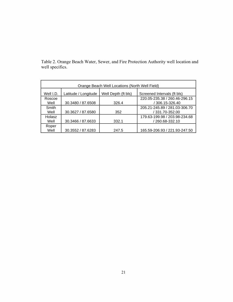
Table 2. Orange Beach Water, Sewer, and Fire Protection Authority well location and well specifics.

Orange Beach Well Locations (North Well Field)

Well I.D. Latitude / Longitude Well Depth (ft bls) Screened Intervals (ft bls) Roscoe

Well 30.3480 / 87.6508 326.4 220.05-235.38 / 260.46-296.15

/ 306.15-326.40 Smith Well 30.3627 / 87.6580 352

205.21-245.89 / 281.03-306.70 / 331.70-352.00

Holasz Well 30.3466 / 87.6633 332.1

179.63-199.98 / 203.98-234.68 / 260.68-332.10

Roper Well 30.3552 / 87.6283 247.5 165.59-206.93 / 221.93-247.50

Figure 6: Distribution of municipal wells located in Foley and Orange Beach, Alabama.

22

23

Groundwater Geochemistry of Baldwin County

Groundwater chemistry data were collected from municipal wells managed by the

Orange Beach Water, Sewer, and Fire Protection Authority, the City of Foley and Riviera

Utilities, and from previous publications (Layne Geosciences, 1997; Goodwyn, Mills and

Cawood, 2000) in the study area. Figure 6 shows the locations of these wells which were

installed in the aquifer zones of A2 and A3. The physio-chemical parameters and major

ion concentrations of the analyzed groundwater samples are shown in Tables 3 and 4.

According to the relative molar proportion of the dissolved ionic species, the

groundwater in the A2 and A3 aquifers in the study area shows mixed nature (Ca-Mg-Na-

K and Cl-SO4-HCO3 types) (Figure 7). The groundwater is composed of varying values

of alkalinity (range: 4.1 to 29.2; mean: 16.65), Na (range: 2.89 to 5 mg/l; mean: 3.95), Ca

(range: 0.78 to 15.2 mg/l; mean: 7.99), Mg (range: 0.55 to 1.86 mg/l; mean: 1.21), Cl

(range: 3.9 to 9.09 mg/l; mean: 6.5), SO4 (range: 3.73 to 12 mg/l; mean: 7.865), and

variable pH (range: 4.2 to 8.58; mean: 6.39). These groundwaters in general have low

ion concentrations; their isotope ages and residence time (see sections below) correspond

to young groundwater of meteoric origin.

24

Table 3. Groundwater major ion data from the Riviera Utilities, City of Foley Wells

Riviera Utilities, City of Foley Production Wells Major Ions

Analyte Symbol Ba Mg Ca Na Zn Mn Cl Fe SO4 Alkalinity pH

Unit Symbol mg/L mg/L mg/L mg/L mg/L mg/L mg/L mg/L mg/L mg/L Wells 7 & 9 <0.05 1.86 15.2 4.31 0.15 0.05 9.09 <0.05 3.73 27 8.58Well 10 <0.05 1.27 14 2.89 0.19 <0.01 5.48 <0.05 <0.05 29.2 8.07

Table 4. Groundwater major ion data from the Orange Beach Water, Sewer, and Fire Protection Authority.

Orange Beach North Well Field Major Ions

Analyte Symbol SO Alkalinity pH Ba Mg Ca Na Zn Mn Cl Fe 4

Unit Symbol mg/L mg/L mg/L mg/L mg/L mg/L mg/L mg/L mg/L mg/L

Smith Well 0.046 0.089 1.3 5 0.022 0.035 3.9 0.97 12 7.8 5.9

Holasz Well 0.024 0.55 0.78 5 0.02 0.01 5.9 0.076 7.8 2.1 4.2

25

Roper Well 6 5.4 4.6 5.1

26

Figure 7: Piper diagram of drinking well water in southern Baldwin County.

27

Saltwater Intrusion in Southern Baldwin County

Previous study (Murgulet and Tick, 2008) conducted in southern Baldwin County

on the A1, A2, and A3 aquifers showed that groundwater near the coastal margin

possesses poor water quality with relatively high total dissolved solids (TDS), salinity,

and chloride concentrations (Figure 8).

In the A1 aquifer elevated levels of TDS, salinity, and chloride were observed.

The average salinity concentrations for aquifer A1 were 1,153.9 mg/L with a maximum

of 18,000 mg/L in close proximity to the coastline (Murgulet and Tick, 2008). Chloride

concentrations for the A1 aquifer were 486.2 mg/L with a maximum concentration of

7,758.3 mg/L in the Gulf Shores area. Average TDS concentrations were 1,359.3 mg/L

with a maximum concentration of 14,590 mg/L (Murgulet and Tick, 2008).

The average salinity concentrations from the A2 aquifer was determined to be

96.8 mg/L with a maximum concentration of 2,590 mg/L and the average chloride

concentrations were 28.2 mg/L with a maximum concentration of 1,460 mg/L (Murgulet

and Tick, 2008). TDS concentrations averaged 146.8 mg/L with a maximum of 3,610

mg/L.

The groundwater samples obtained in the Murgulet and Tick (2008) study in the

A3 aquifer exhibited relatively low concentrations of salinity and chloride compared to

A1 and A2 aquifers. The average salinity concentration was 39.5 mg/L with a maximum

Wolf Bay

Foley

Orange Beach

Aquifer A1 Cl

Aquifer A1 TDS

Aquifer A2 Cl

Aquifer A2 TDS

Figure 8: Contours show the positions of the chloride (250 mg/L) and TDS (500 mg/L) levels equivalent to drinking water limits set by the EPA (data from (Murgulet and Tick, 2008). These lines define the extent of saltwater intrusion occurring in the A1 and A2 aquifers in southern Baldwin County.

28

29

concentration of 136 mg/L and the average chloride concentration was 13.6 mg/L with a

esults from the Murgulet and Tick (2008) study indicate that saltwater intrusion

has occ

rea

roundwater Geochemistry of Dauphin Island

m Dauphin Island were received from the Dauphin Island Water and

Sewer A

loride

urface Water Chemistry of Wolf Bay and Weeks Bay

Data from the surface water sampling in Wolf Bay are shown in Table 7, which

include latitude and longitude, temperature, pH, ORP, conductivity, DO, and turbidity

maximum concentration of 18.2 mg/L (Murgulet and Tick, 2008). TDS concentrations

averaged 51.4 mg/L with a maximum of 190 mg/L north of the Intercoastal Waterway

(Murgulet and Tick, 2008).

R

urred in the A1 and A2 aquifers, as indicated by high levels of chloride and

salinity in wells completed near the Gulf of Mexico. The front of saltwater in the A1

aquifer, as defined by the 250 mg/L chloride isochlor, already approaches the inland a

near Foley (Figure 8).

G

Data fro

uthority. Dauphin Island currently has eight shallow wells in production.

Chloride data was collected and Table 6 shows pre- and post- hurricane Katrina ch

levels in the wells. Table 7 shows the well locations and specifics of the shallow

production wells.

S

30

from th

to

-

DO

e July 2008 cruise survey. Measurements were taken at different depths to

delineate the spatial distribution of the bay’s water quality. The surface water near the

Intercoastal Waterway (WB-1 through WB-10) is characterized by higher pH (7.75

7.93), higher temperature (29.05 to 31.72 °C) and high conductivity (32,990 to 36,050

µS/cm). In contrast, surface waters near the input of Wolf Creek (WB-24 through WB

31) into the bay have relatively lower pH (7.55 to 7.74), lower temperature (27.47 to

29.98 °C) and lower conductivity (22,980 to 33,800 µS/cm). The surface water sampled

near the Wolf Creek mouth (where creek water mixes with bay water) has the lowest

and ORP values (as shown in Table 7).

31

able 5. Chloride levels in selected Dauphin Island wells pre- and post- hurricane Katrina (2005).

-03 Jul-06 Aug-06 Oct-06 May-07

T

Sep

WELL #10 40 320 380 360 320

WELL #20 25 180 200 180 140

WELL #30 20 300 320 180

Jul-92 Sep-0 Aug-0 Oct-07 Dec-07 7 7 May-07

WELL #50 39 30 100 80 60 60

WELL #60 46 30 100 120 80

WELL #70 0 48 30 60 80 6 60

WELL #80 26 30 50 100 80 80

32

Table 6. Dauphin Island Water and Sewer Authority well locations specifics.

Dauphin Island Water and Sewer Authority Shallow Production Wells

Well I.D. Latitude / Longitude Well Depth (ft bls) Screened Interval (ft bls)

#10 30.25380 / 88.11003 30 18-28

#20 30.25156 / 88.10153 32.5 20.5-30.5

#30 30.25124 / 88.9686 34.5 22.5-32.5

#40 30.25168 / 88.10746 33 21-31

#50 30.24913 / 88.10757 40 23.65-33.65

#60 30.249 24.75-34.75 40 / 88.10377 40

#70 30.24767 / 88.09223 40 26.10-36.10

#80 30.24676 / 88.09223 40 26.65-36.65

33

or comparison, surface water data collected from Wolf Bay (this study) and

Weeks ater

s of

F

Bay (Monrreal, 2007) are shown in Tables 7 and 8. In Weeks Bay, the river w

and surface water near the river mouth are characterized by relatively low pH (5.99 to

6.54), low temperature (27.80 to 31.65 °C), and low conductivity (138 to 2017 µS/cm).

The surface waters near the bay mouth however, have relatively high pH (7.8 to 8.75),

high temperature (32.0 to 33.25 °C), and high conductivity (3350 to 5706 µS/cm).

Conductivity of water in Weeks Bay is much lower than that in Wolf Bay. pH value

surface water in the upper Weeks Bay near the river mouth are also significantly lower.

The surface water sampled near the river mouth where river water mixes with bay water

has the lowest DO and ORP values generally. The major ion composition of surface

water is shown in Table 9.

34

able 7. Surface water chemistry from locations within Wolf Bay taken at surface level, collected in July, 2008.

I.D. Latitude Longitude pH Conductivity ORP D.O. Temperature Turbidity

T

Sample

WB-1 30.1805 87.08734 7.92 36050 161 5692 31.72 12.8WB-2 30.1807 87.34482 7.93 35000 176 6644 31.2 11.2WB-3 30.3015 87.58907 7.9 34220 71 7130 30.15 14.8

WB-4 30.3019 87.59952 7.8 32990 69 6972 30.27 13.4WB-5 30.3049 87.59916 7.8 34360 26 7090 30.6 13.4WB-6 30.3054 87.59403 7.79 34810 48 7149 31.65 10.1WB-7 30.3058 87.58722 7 29.86 .81 35090 66 7151 10.3

WB-8 30.3057 87.58235 7.74 34530 73 7568 29.05 11WB-9 30.3102 87.58242 7.8 34590 81 7095 30.75 9

WB-10 730.3102 87.58625 7.75 35190 86 7122 30.88 .5

WB-11 30.3098 87.59225 7.82 35030 103 6730 30.64 9.4

WB-12 30.3097 87.59503 7.75 34780 102 7025 30.21 8.7WB-13 30.3147 87.59267 7.62 34840 121 7023 28.36 8.1WB-14 30.3156 87.58917 7.65 34330 116 7110 29.54 7.7

WB-15 30.3166 87.58405 7.66 34120 125 6791 28.92 8.9WB-16 30.3238 87.5858 7.5 34380 121 7228 27.27 6.2

WB-17 30.3239 8 77.58946 .67 32780 127 6329 30.43 7.2

WB-18 30.3233 87.59389 7.74 32680 123 7160 28.35 6.7

WB-19 30.3277 87.59825 7.73 32750 81 6977 29.67 7.7WB-20 30.3295 87.59083 7.78 32910 119 6937 29.58 8.2WB-21 30.3342 87.58184 7.76 34070 121 6203 29.73 7.3WB-22 30.3345 87.5787 7.79 34060 131 6362 27.59 7.1WB-23 30.3412 87.58103 7.75 33570 104 6928 27.41 8.1WB-24 30.34 87.58235 7.74 33800 112 7060 28.16 9.7

WB-25 30.3376 87.58406 7.72 33790 -23 6766 29.44 13.14WB-26 30.334 87.58916 7.61 33580 60 5587 27.47 3.2WB-27 30.3334 87.59186 7.66 33080 94 6866 29.48 10.6WB-28 30.3363 87.59828 7.58 29420 97 7777 29.81 7.2

WB-29 30.3379 87.59815 7.59 29200 106 6750 27.81 7.2

WB-30 30.3408 87.60319 7.6 23660 97 6772 29.72 9.6WB-31 30.3451 87.60119 7.55 22980 114 7463 29.98 7.8

35

able 8. Surface water chemistry collected from locations within Weeks Bay and Fish iver taken at surface level in July 2005 (from Monrreal, 2007).

Temperature Turbidity

TR

Sample I.D. Latitude Longitude pH Conductivity ORP D.O.

WB1-S 30.4133 87.8255 6.47 909 540 5950 30.93 22.4

WB2-S 7 6.4130.4094 87.82658 942.6 609 5020 31.65 22.5

WB3-S 30.37686 87.8358 8.49 5700 533 6700 32.82 19.9WB4-S 30.38289 87.8348 8.6 5522 467 7394 32.89 21.6

WB5-S 30.39041 87.8331 8.77 5174 493 8100 33.56 17.6

WB6-S 30.3981 8 87.83061 .43 2715 384 6360 33.02 23.3

WB7-S 30.40286 87.82869 6.28 300 488 4455 31.5 19.8WB8-S 30.40080 87.82963 6.6 1311 518 5498 32.16 19.7

WB9-S 30.40722 87.82736 6.38 204 502 6233 32.17 22

WB10-S 30.38963 87.81616 7 3000 457 5038 32.0 29

WB11-S 30.39219 87.82005 8.0 32.66 29 3975 432 6330 8.2WB12-S 30.39319 87.82469 8.62 32.60 24.14002 381 7360

WB13-S 30.39389 87.82908 8.66 5136 365 6110 33.17 19.8

WB14-S 30.39525 87.83678 8.3 2340 356 6658 32.66 18

WB15-S 30.39685 87.84175 8.06 1865 361 7150 32.69 31

WB16-S 30.39091 87.84086 8.41 19.92880 344 6800 33.06

WB17-S 30.38669 87.84013 8.75 3350 327 7356 33.22 23.3

WB18-S 30.38302 87.83894 8.79 3255 324 7746 33.22 21WB19-S 30.37844 87.83705 8.8 3436 330 7815 33.25 20.9

WB20-S 30.40122 87.83738 8.19 2108 290 7255 33.63 24.4

WB21-S 30.40672 87.83422 6.69 560 386 5369 32.72 26.2

WB22-S 30.41030 87.82988 7.03 1119 409 7150 31.99 29.9

FISH1-S 30.44500 87.80433 6.8 66.01 403 8851 31.4 9.9

FISH2-S 30.44272 87.80280 6 31.54 .63 65.31 482 8805 9.5

FISH3-S 30.44361 87.80728 6.57 63.97 514 9043 30.2 10.7FISH4-S 30.44083 87.81160 6.9 71.4 455 9210 31.98 13.1

FISH5-S 30.43600 87.81261 6 6.98 9.26 447 9500 31.83 12.9

FISH6-S 30.43563 87.81891 6.82 76.5 454 9540 31.65 15

FISH7-S 30.43130 87.82372 6.83 98.3 443 9140 32.17 13.9FISH8-S 30.42750 87.82855 6.61 105.2 444 8600 31.97 14.6

FISH9-S 30.42411 87.82477 6.7 123.3 441 8659 32.50 15.6

36

Table 9. Major ion composition of surface water collected from Wolf Bay.

K Mg Ca Na S Sr Cl Br SO4 Analyte Symbol Unit Symbol /L /L L L L mg mg/L mg/L mg/L mg µg/ mg/ mg/ mg/LAnalysis Method

ICP- OES

ICP- OES

ICP- OES

ICP- OES

ICP- OES

ICP- OES IC IC IC

WB-10 306 00 0 0675 234 6830 536 3580 106 < 1 152WB-14 282 625 215 6380 493 3320 11000 < 30 1520WB-19 272 613 208 6130 489 3260 6800 26.1 949WB-21 270 613 210 6150 483 3270 9750 < 110 390WB-23 262 595 206 5950 468 3250 1 80700 37. 1510WB-28 248 573 198 5800 455 3030 9870 35.9 1370

WB-31 267 608 208 6080 473 3230 10700 38.9 1490

37

DISSCUSSION

Water chemistry is an important factor in the methylation and bioaccumulation of

mercury. Conditions are constantly changing especially in estuary environments and can

affect the fate and biotransformation of Hg. Data collected from the previous studies

conducted in Weeks Bay and this study in Wolf Bay reveal how the difference in the

hydrodynamics of the bays affects water chemistry and mercury methylation. Water

samples were also collected for isotope and chemical analysis to investigate how water

mixing and evaporation affects the water chemistry in the watershed. From the collected

field data, GIS-based computer models were created to help interpret the mixing of

surface water and seawater and the degree of evaporation in the bays. The Wolf Bay data

were compared to the Weeks Bay data and analyzed to help obtain a better understanding

of the water mixing within the bays and how that affects the methylation of mercury.

Mercury Deposition and Precipitation

Mercury deposition data from the Mercury Deposition Network (MDN) site AL02

(Figure 9) (http://nadp.sws.uiuc.edu/mdn) were compared with USGS precipitation data

from the same time periods reported in Monrreal (2007) to show possible correlations

between mercury deposition and precipitation for the area near the Weeks Bay and Wolf

Bay watersheds. Figure 10 shows that total mercury wet deposition increases with the

amount of weekly atmospheric precipitation.

Figure 9: Map of location of MDN sampling sites in the southeastern region of the United States (http://nadp.sws.uiuc.edu). Data from sites AL02 were used for analysis of Hg deposition near Wolf and Weeks bays.

38

Date

Hg

Dep

ositi

on (n

g/m

2 )

0

200

400

600

800

1000

1200

1400

1/9/2007 2/13/2007 3/20/2007 4/24/2007 5/29/2007 7/3/2007 8/7/2007 9/11/2007 10/16/2007 11/20/2007 12/26/2007-1

0

1

2

3

4

5

6

7

8

Prec

ipita

tion

(inch

es)

Figure 10: Fluctuations of total mercury wet deposition (collected by the Mercury Deposition Network, MDN) responding to rainfall in southwestern Alabama from January 2007 to January 2008. Rainfall data (vertical bars, in inches) were collected along the Fish River. The diagram shows increased mercury deposition during periods of higher precipitation, suggesting atmospheric deposition of mercury pollution.

39

40

The correlation of mercury wet deposition and precipitation data confirms that the likely

source of mercury in Weeks Bay and Wolf Bay watersheds is atmospheric mercury

deposition.

Surface Water Chemistry

Chemistry data of surface water demonstrates a mixing zone in Wolf Bay and

Weeks Bay, resulting from seawater intrusion along the bottom of the bay. Grouping of

different geochemical characteristics (Figures 11-14) indicate that those waters have

distinct chemical characteristics, such as pH, conductivity, D.O., and temperature.

Seawater has higher temperatures, pH, and electrical conductivity.

The chemistry data from the surface water samples show a mixing zone in Wolf

Bay as a result of seawater intrusion along the lower portion of the bay. The geochemical

analysis shows elevated chloride levels, which suggest that the bay has been

contaminated by seawater. The intrusion of seawater into the bay creates a front of high

salinity, high pH water that is denser and able to wedge underneath the lighter, low-

conductive freshwater. Changes occur in water chemistry at the freshwater/saltwater

interface and cause the bay to have pronounced stratifications due to the influx of

seawater.

Each type of water has certain characteristics to fingerprint their origin such as

pH, conductivity, D.O. and temperature. Mercury methylation favors waters with higher

41

temperatures, lower pH, and lower salinity (or electrical conductivity). Surface water near

the Intercoastal Waterway has the highest pH, temperature, and conductivity values. By

comparing these parameters from Wolf Bay to Weeks Bay it may help to explain the

spatial distribution of mercury methylation and its relation to the mixing of seawater,

river water, and groundwater in the bays and the difference of the bays.

By comparing the data collected in Wolf Bay there appears to be a transition

between the waters entering Wolf Bay from fresh water sources and that of the saline

water in the bay itself. Measurements of pH and conductivity taken along a north-south

transect from the mouth of Wolf Creek to the Intercoastal Waterway show a trend of high

conductive, high pH seawater entering the bay (Figures 15 and 16). The data collected at

lower depth have a higher pH and conductivity than those of the surface water. This

trend suggests that the higher pH and higher conductive, denser seawater is intruding

along the bottom of the water column in the bay and mixing with the lower pH and lower

conductive waters from the creeks flowing into Wolf Bay. The pH, temperature and

conductivity data collected at the surface and 1 meter depths in Wolf Bay also show the

similar trend (Figures 17-20). Contour gradients of conductivity, temperature, and pH

are more pronounced in the upper bay which indicates that a saline wedge has formed by

the mixing of saltwater and freshwater. Waters at depth are more saline and warmer than

those at the surface which is another indicator that dense seawater is intruding farther into

Wolf Bay at depths below relatively fresher surface water. The plots illustrate that warm

dense seawater invades beneath cooler fresh waters from the creeks that feed Wolf Bay.

The saltwater wedge formed within Wolf Bay is indicated by the presence of the

42

temperature and salinity stratifications. Previous studies in different watershed basins

suggest that the highest mercury methylation primarily occur near the saline wedge,

where lower pH water and low-salinity water are both present by mixing. The

conductivity values in Wolf Bay (ranging from 22,980 to 36,050 µS/cm) appear to be

much higher than those in Weeks Bay (ranging from 63.97 to 5700 µS/cm). This high

salinity implies a less favored condition for Hg methylation (Ullrich et al., 2001; Celo et

al., 2005; and Monrreal, 2007). pH values show greater variations in Weeks Bay than

those in Wolf Bay, probably reflecting stronger mixing and freshwater inputs in the

Weeks bay watershed.

The ORP and DO contour maps show areas of Wolf Bay that exhibit spatial

variations in oxidized or reduced conditions (Figure 21). Some bacteria, such as sulfate

reducing bacteria (SRB), prefer anaerobic waters with low ORP values that may

contribute to the methylation of mercury (King et al., 2002; Monrreal, 2007). The lowest

ORP values are located near the mouth of Wolf Creek, near the interface of fresh and

brackish waters. Water DO and ORP values in Wolf Bay are comparable to those of

Weeks Bay. However, in Weeks Bay low DO levels and reducing conditions prevail in

the mixing zone near the mouth of Fish River. The reducing conditions in Weeks Bay

may indicate more intensive microbial activity, which is an important factor in the

methylation of mercury.

0

5000

10000

15000

20000

25000

30000

35000

40000

6 6.5 7 7.5 8 8.5 9

pH

Con

duct

ivity

Wolf Bay

Weeks Bay

Figure 11: Plot of pH vs. conductivity showing a general relationship in water chemistry parameters that demonstrate the differences in the Wolf Bay and Weeks Bay waters.

43

0

5000

10000

15000

20000

25000

30000

35000

40000

0 2000 4000 6000 8000 10000 12000

D.O.

Con

duct

ivity

Wolf Bay

Weeks Bay

Figure 12: Plot of conductivity vs. DO comparing the water chemistry parameters from locations within Wolf Bay and Weeks Bay.

44

6

6.5

7

7.5

8

8.5

9

29.00 30.00 31.00 32.00 33.00 34.00

Temperature

pH

Wolf Bay

Weeks Bay

Figure 13: Plot of temperature vs. pH comparing the relationship in the mixing of the

45

water within Wolf Bay and Weeks Bay.

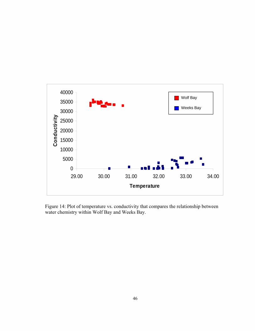
46

ater chemistry within Wolf Bay and Weeks Bay.

Figure 14: Plot of temperature vs. conductivity that compares the relationship between

0

5000

10000

15000

20000

25000

30000

35000

40000

29.00 30.00 31.00 32.00 33.00 34.00

Temperature

Con

duct

ivity

Wolf Bay

Weeks Bay

w

47

Figure 15: Plot of pH values at three different depths along a north-south transect from

6.5

7

7.5

8

8.5

9

050

010

0012

5017

5022

5027

5035

0045

0055

00

Distance (meters)

pH

the mouth of Wolf Creek to the Intercoastal Waterway. The higher pH water is near the Intercoastal Waterway and the invasion of seawater into Wolf Bay creates a saltwater front.

Surface1 m2 m

Wolf Creek

Intercoastal Waterway

48

Figure 16: Plot of conductivity values at the surface along a north-south transect from e mouth of Wolf Creek to the Intercoastal Waterway. The increase in conductivity

y.

2200024000260002800030000320003400036000380004000042000

050

010

0012

5017

5022

5027

5035

0045

0055

00

Distance (meters)

Con

duct

ivity

(uS

/cm

)

thindicates a high salinity front which is created by the intrusion of seawater into Wolf Ba

Surface1 m2 m

Wolf Creek

Intercoastal Waterway

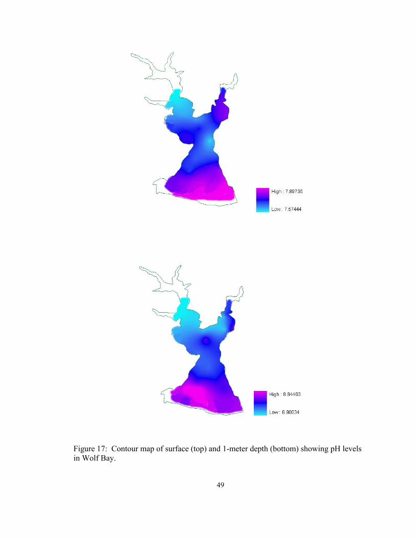
Figure 17: Contour map of surface (top) and 1-meter depth (bottom) showing pH levels in Wolf Bay.

49

Figure 18: Contour maps of surface (top) and 1-meter depth (bottom) showing temperature (°C) levels in Wolf Bay. Like the pH readings, higher temperature water can be found closer to the Intercoastal Waterway.

50

Figure 19: Contour map of surface (top) a -meter depth of conductivity levels (in µS/cm) in Wolf Bay. Similar to temperature and pH, higher conductivity readings can be found near the Intercoastal Waterway.

nd 1

51

Figure 20: Contour map of (surface) and 1-meter depth of DO levels. Th highest DO readings are located at the mouth of W lf Creek.

e o

52

Figure 21: C of ORP. Lowest ORP zones are found at the mouth of Wolf Creek.

ontour map of surface (top) and 1-meter depth (bottom)

53

Figure 22 shows the geochemical characteristics of sampled waters in Wolf

Bay and Weeks Bay using a piper diagram. The surface waters in Wolf Bay and

Weeks

)

ks Bay contains high amounts of Na and

HCO3- which indicates sodium bicarbonate type of groundwater. The Na-HCO3 type

high alk

Bay both contain high amounts of Na and Cl, similar to the characteristics of

seawater. The Wolf Bay surface water has the same SO4/Cl ratios (average 0.052

with respect to that of seawater (~0.052), suggesting that dissolved SO4 in Wolf Bay

has not been affected by bacterial sulfate reduction, a key process for initializing Hg

methylation. By contrast, very low SO4/Cl ratios are found in Weeks Bay where Hg

methylation has occurred (Monrreal, 2007).

The groundwater analyzed from Wee

alinity of the groundwater in Weeks Bay is most likely a result of the

combination of dissolution of calcite and ion exchange (Marimuthu, 2005; Penny et

al., 2005; and Monrreal, 2007).

54

Figure 22: Piper diagram showing surface and groundwater compositions compared to that of seawater. Surface waters resemble those of seawater (i.e., Na-Cl types).

55

Major ion analyses can also aid in providing more information on the physical

ixing and biogeochemical reactions that take place in the bays. Graphs were plotted

to evalu

e

een

seawater and freshwater in Weeks Bay, while more non-conservative mixing can be

found i ions

m

ate the mixing of the waters and compared to each other (Figures 23-26). In

the plots, chloride, a conservative (non-reacting) species, is plotted on the x axis. The

other species of interest, which may or may not be conservative, is plotted on the y

axis. A straight line was drawn between the seawater and freshwater end-members

and the behavior was based on the proximity of the data points to the line. If those

data points lie close to or on the mixing line, that indicated the dissolved species

exhibit a more conservative behavior. Data points that deviate significantly from th

conservative mixing line are considered non-conservative. The species enrichment or

depletion is in solution may be dependent upon biogeochemical processes such as

mineral dissolution or precipitation, ion-exchange, or microbial processes.

In all of the graphs, linear trends reveal the conservative mixing betw

n Wolf Bay. Wolf Bay waters in general have higher major ion concentrat

with respect to those in Weeks bay because of less freshwater inputs. The results of

the graphical analyses indicate Na+ +2, Ca , Mg+2 generally exhibit conservative

behavior during mixing in Weeks Bay and less conservative behavior in Wolf Bay.

56

0

5

10

15

20

25

30

35

40

45

4000 5000 6000 7000 8000 9000 10000 11000 12000

Chloride (ppm)

Bro

mid

e (p

pm)

Wolf Bay

Figure 23: Plot of chloride vs. bromide showing a more linear pattern between the water in Weeks Bay and less in Wolf Bay.

Weeks Bay

Weeks Bay

Wolf Bay

57

0

50

100

150

200

250

300

4000 5000 6000 7000 8000 9000 10000 11000 12000

Chloride (ppm)

Cal

cium

(ppm

)

Weeks Bay

Wolf Bay

Figure 24: Plot of chloride vs. calcium showing similar patterns between waters.

58

0

100

200

300

400

500

600

700

800

900

4000 5000 6000 7000 8000 9000 10000 11000 12000

Chloride (ppm)

Mag

nesi

um (p

pm)

Weeks Bay

Wolf Bay

Figure 25: Plot of chloride vs. magnesium with a similar pattern between Weeks and Wolf Bay.

59

Figure 26: Plot of chloride vs. sodium showing the linear pattern of waters within Weeks Bay and the waters of Wolf Bay.

0

1000

2000

3000

4000

5000

6000

7000

8000

4000 5000 6000 7000 8000 9000 10000 11000 12000

Chloride (ppm)

Sodi

um (p

pm)

Weeks Bay

Wolf Bay

60

0

200

400

600

800

1000

1200

1400

1600

5000 6000 7000 8000 9000 10000 11000 12000

Chloride (ppm)

SO4 (

ppm

)

Wolf Bay

Weeks Bay

Figure 27: Plot of chloride vs. SO4 showing the linear pattern of waters within Weeks and Wolf Bay.

61

Interestingly, sulfate exhibits non-conservative depletion in Weeks Bay (about

0%) and more conservative in Wolf Bay (Figure 27). Bacterial sulfate reduction in

Weeks

ry in the areas

of freshwater tributaries according to previous studies. In the

previou

noit

t

1

Bay may be the reason for this depletion but more microbiology research is

needed to verify the biogeochemical reactions that remove sulfate.

Estuary environments show the highest levels of methylmercu

near the mouths

s studies, the upper estuaries of freshwater/saltwater mixing zone contained

low DO levels, low pH, and low salinity (Baeyens, 1998; Benoit, 1998; and

Leermakers, et al., 2001). These conditions are ideal for sulfate-reducing bacteria to

exist which have been shown to play a part in the methylation of mercury (Be

2001; King, 2002; and Monrreal, 2007). These same desired geochemical conditions

may exist within Weeks Bay near the mouth of the Fish River (Monrreal, 2007), bu

not in Wolf Bay where water salinity is too high.

62

Table 10. Oxygen and hydrogen isotope composition of groundwater, bay water, and ver water in Wolf and Weeks Bay watersheds.

Name Source O, /00

(SMOW) δD, /00

(SMOW)

ri

Sample Water δ18 0 0

9 Transition Zone -2.1 -14.9 011A 011B

W W

14 Weeks Bay -1.5 -10.1

W W W W

TraTra

Sea Water

eeks Bayeeks Bay

-1.2 -1

-7.5 -9.6

18 Fish River -2.3 -11.9 23 Fish River -2.2

--15.5

27 Fish River 2.7 -16.5 28 Weeks Bay -2.3 -15.6 33 Weeks Bay -1.8 -9.4 38 Weeks Bay -1.6 -8.1 41 Weeks Bay -1.6 -6.3 41 Weeks Bay -1.5 -4.3 W13 Groundwater -4.4 -23.1 W14 Groundwater -4.1 -26.6 W15 Groundwater -2.7 -17.3 W16 Groundwater -4.4 -26.9

-1.7 -6.7 WC-1 Wolf Creek -1.5 -9.7 WC-2 Wolf Creek

WB10 Wolf Bay 0.3 -0.2 WB12 Wolf Bay 0.3 -0.3 WB14 Wolf Bay -1.6 -0.3 WB16 Wolf Bay -1.6 -0.3 WB19 Wolf Bay -0.4 -0.4 WB21 Wolf Bay 0.8 -0.3 WB23 Wolf Bay -1.1 -0.4 WB26 Wolf Bay 1.8 -0.4 WB28 Wolf Bay -0.5 -0.6 WB30 nsition Zone -0.6 -0.5 WB31 nsition Zone -0.9 -0.5

0 0

63

Stable Isotope Signatures of Stream Water, Bay Water, and Groundwater

and

emonstrates the role that water mixing (i.e., with groundwater and seawater) and

evapora

r

n

r”

by

ulf

Stable isotope analyses provides more details about the mixing of waters

d

tion play in influencing the chemistry of Wolf Bay and Weeks Bay surface

water. Comparing oxygen and hydrogen isotopes of surface water and groundwate

sampled sites along with seawater signature as well as the local meteoric water line

shows how mixing and evaporation affect water chemistry in both bays (Figure 28).

Deuterium (δD) and oxygen (δ18O) isotope ratios of groundwater and surface water i

Wolf and Weeks Bay are plotted along with seawater and evaporation trajectory of

the local meteoric water line (LMWL). Evaporation preferentially lifts lighter 16O and

1H isotopes from water to atmosphere. As evaporation occurs in surface waters, the

remaining waters become enriched in heavy isotopic (18 2O and H) composition.

Seawater is enriched with 18 16O and O with respect to surface meteoric water. Stable

isotope signatures of groundwater fall close to the local meteoric water line,

indicating very little to no evaporation or mixing prior to infiltration from pore water

in the unsaturated zone. In contrast, stable isotope profiles of river water show

enrichment of 18 2O and H, indicating they undergo greater evaporation than

groundwater. The Weeks Bay water represents a mixture of three “end-membe

waters: one of seawater, one of river water, and one of groundwater impacted

variations in evaporation rates. Wolf Bay water plots closer to the seawater which

represents greater evaporation rates and/or more influence of seawater from the G

of Mexico. Isotopic signatures of Wolf Bay water also indicate less input from

64

surface (meteoric) with respect to Weeks Bay, which is consistent with its high

electrical conductivity and salinity nature. The nature and extent of hydrologic

mixing and evaporation strongly influence water quality in both bays, which has

profound impacts on the potential of Hg methylation in bays.

65

Seawater

mixing

evaporation

Figure 28: Plot of evaporation trajectory of local meteoric water line (LMWL) and seawater mixing trend, shown using deuterium (δD) and oxygen (δ18O) isotope ratios of groundwater and surface water in Wolf Bay. The Weeks Bay water represents a mixture of three “end-member” waters: one of seawater, one of river water, and one of groundwater impacted by variations in evaporation rates. Wolf Bay water plots closer to the seawater which represents greater evaporation rates and/or more influence from the Gulf of Mexico.

66

SUBSURFACE GEOPHYSICAL SURVEY

Electrical Resistivity

Electrical resistivity surveys were performed on Dauphin Island at the Isle

Dauphin golf course (Figure 29) and at Gulf State Park, located near Orange Beach

(Figure 30). A 48-channel AGI SuperSting® Automated Resistivity Meter was used

for these surveys. A 2-D dipole-dipole array was used, with an electrode spacing of

three meters along the survey transect. A roll-along technique was used to extend

each transect to 450 meters at Dauphin Island and 450 meters at Gulf State Park. The

transects were geo-referenced using a sub-meter accuracy Trimble GPS.

Field data were processed using the EarthImager2D resistivity processing

software. Results were interpreted to estimate the depth to the saltwater interface or

areas of saltwater intrusion. The measured apparent resistivity, calculated apparent

resistivity, and the calculated true resistivity along the transect are shown in Figure 31

for Dauphin Island and Figure 32 for Orange Beach.

Resistivity of water may vary from 0.2 to over 1000 Ω m depending on its

ionic concentration and the amount of dissolved solids, and average seawater has a

resistivity of 0.2 Ω m (Nowroozi et al., 1999). Resistivity of natural water and

sediments without clay may vary from 1 to 100 Ω m while the resistivity of a layer

saturated by saline water and some dissolved solids is in the range of 8 to 50 Ω m (De

67

Breuk and De Moor, 1969, Sabet, 1975, Goodell, 1986, Flanzenbaum, 1986, Zohdy et

al., 1993, Nowroozi et al., 1999).

In the Dauphin Island profile (Figure 31) resistivity ranged from 0 to over

6000 Ω m. In the shallow subsurface the data yielded a wide range of resistivity

readings. The higher readings probably reflect unsaturated unconsolidated sediments.

The lower readings, especially in the 6-to 20-meter depth range, may indicate

possible saltwater encroachment (indicated by arrows in Figure 31). These anomalies

of low resistance may be the result of possible saltwater contamination within the

shallow groundwater that percolated from the surface after the hurricane Katrina

storm surge. The true freshwater-saltwater interface was not located. In order to

detect the interface using this method, a longer transect will need to be performed to

achieve a greater depth in the survey. These results imply that the depth of the

saltwater wedge is greater than 50 meters.

In the Orange Beach profile (Figure 32) resistivity ranged from 223 to 4444 Ω

m. These readings appear to indicate the high resistance of unsaturated layers. The

survey was conducted on a golf course with multiple groundwater wells that provide

irrigation to the course and it was also conducted during a drought. With the

groundwater withdrawal from the wells and little to no recharge, groundwater may

have been at a greater depth. The depth of the freshwater-saltwater interface was

greater than anticipated therefore further studies should be conducted employing a

68

longer transect in order to increase the depth of coverage and possible detection of the

freshwater-saltwater interface.

69

1 km

Figure 29: Location of geophysical survey at Dauphin Island, Alabama.

70

1 km

Figure 30: Location map of geophysical survey at Orange Beach, Alabama.

71

0 50 100 150 200 250 300 350 400 450

Dauphin Island Electrical Resistivity Survey

Ohm-m

S N

Figure 31: Results from electrical resistivity survey at Dauphin Island. The transect used an electrode spacing of 3 meters. Arrows are pointing to the low resistive anomalies in the survey. The error limit of the data was 2.72 %, which is in the acceptable range as stated in Advanced Geosciences Inc. (2002). The true resistivity was calculated using EarthImager 2D. (Profile location is located in Figure 29).

72

0 50 100 150 200 250 300 350 400 450 Ohm-m

Orange Beach Electrical Resistivity Survey

S N

Figure 32: Results from electrical resistivity survey at Orange Beach. The transect used an electrode spacing of 3 meters. The error limit of the data was 2.74 %, which is in the acceptable range as stated in Advanced Geosciences Inc. (2002). The true resistivity was calculated using EarthImager 2D. (Profile location is located in Figure 30).

73

HYDROLOGIC MODELS

Surface Flow of Wolf Creek and Fish River

To understand and compare the influx of freshwater into Wolf Bay and Weeks

Bay, data collected by the United States Geological Survey (U.S.G.S.) was obtained

to compare the surface water flow into the bays (Figure 33). The USGS WaterWatch

website (http://waterwatch.usgs.gov/) provides real-time, short-term (hourly) changes

in gaged rivers and streams. Figure 33 shows stream discharge (ft3/sec) computed at

two USGS gage stations in 2010 at Wolf Creek (station ID 02378170), a major

tributary stream of Wolf Bay, and Fish River (station ID 02378500), a major tributary

of Weeks Bay. The computed USGS data show that stream discharges are much

higher (∼100 ft3/sec) in Fish River than those of Wolf Creek (around 10 ft3/sec). The

high freshwater inflow allows a low-salinity water body to lie on the top of the

invading salinity seawater to form a wedge interface (Figure 15). The mixing of

warm, acidic, and low-salinity waters in the upper Weeks Bay (near the mouth of the

Fish River) may provide favorable conditions for Hg methylation, as observed in the

field. In Wolf Bay, by contrast, less freshwater inflow results in high-salinity of

water throughout the bay, which in turns prevents key microbial processes that

initialize Hg methylation and bioaccumulation. The result suggests that Hg

biotransformation is strongly influenced by hydrochemical conditions (i.e., mixing of

freshwater and saltwater) in coastal watersheds.

74

0

20

40

60

80

100

120

140

160

3/27/2

010

3/29/2

010

3/31/2

010

4/2/20

10

4/4/20

10

4/6/20

10

4/8/20

10

4/10/2

010

4/12/2

010

4/14/2

010

4/16/2

010

4/18/2

010

4/20/2

010

4/22/2

010

4/24/2

010

4/26/2

010

Dish

arge

(cub

ic fe

et p

er s

econ

d)

0

2

4

6

8

10

12

14

16

3/27/2

010

3/29/2

010

3/31/2

010

4/2/20

10

4/4/20

10

4/6/20

10

4/8/20

10

4/10/2

010

4/13/2

010

4/15/2

010

4/17/2

010

4/19/2

010

4/21/2

010

4/24/2

010

Disc

harg

e (c

ubic

feet

per

sec

ond)

Figure 33: Hydrographs of Fish River (top) and Wolf Creek (bottom) showing discharge in cubic feet per second. (Data collected by U.S.G.S.)

75

Regional Groundwater Flow and Groundwater Residence Time

Figure 34 shows the measured water table elevations (Chandler, 1985) and

simulated groundwater flow patterns in southern Baldwin County. Groundwater flow

directions were drawn using SURFER software. Groundwater recharges at high

elevations in the northern part of the study area near Loxley and migrates in the

general direction of south toward the coastal areas. Moderate hydraulic gradients (on

the order of a few m/km) exist in shallow aquifers in the study area. Although

hydrologic properties (e.g., permeability) of the aquifers remain poorly unknown,

available groundwater radioactive isotope data suggest moderate groundwater

discharge rates of a few meters per year (see section below).

A regional basin hydrology program Basin2 was used to simulate groundwater

flow direction and also to calculate groundwater residence time by using the transport

and decay of 36Cl through the aquifers. The program uses a finite-difference grid

which consists of nodal blocks that are arranged into columns and rows and cover a

two-dimensional basin cross-sectional area. Each nodal point contains the properties

of each block. Basin2 calculates a number of variables such as temperature, pressure,

solute (Cl) concentration, and isotopic compositions at each nodal point. The

software is able to model the hydraulic characteristics and isotope transport capability

of the aquifers.

76

Basin2 requires the construction of a cross-section that represents the

stratigraphy and lithology of the basin in order to simulate groundwater flow. The

data for the cross-section was entered in Basin2 in a column format which consisted

of thickness and lithologic composition (see attached CD). Thickness and

composition of each unit was collected from previous stratigraphic data (Mooty,

1988). Basin2 uses three default lithologies (sandstone, shale, and carbonate) that can

be entered into the model.

Groundwater flow and residence time in Baldwin County was modeled in

two-dimension using a basin-scale groundwater flow model Basin2. The Basin2

model calculates groundwater flow resulting from density variation, sediment

compaction, topographic relief, and the transport of heat in the basin strata. The

simulation considers the regional flow in response to topographic relief and water

table variations cross southern Baldwin County from Bay Minette to Orange Beach.

Subsurface data from Chandler et al. (1985) were used to reconstruct the

hydrostratigraphy in the cross section (Figure 35).

77

45

25

0

Contour Interval (m)

Figure 34: Equipotential map of southern Baldwin County, Alabama. Groundwater flows to the south towards the Gulf of Mexico. Also, notice how groundwater is flowing into Weeks and Wolf Bay.

78

The hydrostratigraphy units used in the model include sand, clay, and

carbonate. Permeability of sand, clay, and carbonate are set to 10, 10-4, and 10-2

darcy, respectively. The permeability of the sandy aquifers (Aquifer zones A1, A2,

and A3) is adjusted to reflect the transport characteristics of these aquifers and the

short groundwater residence time (Figure 35). The variations (and uncertainty) on

permeability of clay and carbonate have little effects on groundwater flow in sandy

aquifers. The sides of the basin remain open to groundwater flow. The bottom of the

cross-section is set to be a no-flow boundary to reflect the low-permeability pre-

Oligocene basement rocks. The input file for simulation is shown in Appendix A.

Simulation shows that groundwater migrates in the general direction to the

south towards the Gulf of Mexico in all three major aquifer zones (Figure 35). The

model also predicts that local groundwater flow system may exist in the shallow

aquifer (i.e., Aquifer A2) where pronounced local topographic relief exists and causes

undulations in the water table. Such local and shallow groundwater flow system has

recharge areas near a local topographic high spot and a discharge area at the adjacent

topographic low. The model predicted flow velocities are on the order of a few to

tens of meters per year. The extension of the local flow system is limited to shallow

depths (on the order of a few hundreds of meters) and the deeper A3 aquifer is

dominated by regional flow system with more consistent north-to-south flow

directions. It is expected that groundwater residence time of deeper regional flow is

much longer than those of shallow local flow systems.

79

In Aquifer A1, the velocity arrows show that the groundwater is discharging

to the surface, near the shore of the Gulf of Mexico. Groundwater in the Aquifer A2

flows to the south and then flow upwards into the A1 aquifer around the discharge

area. Groundwater flow in the aquifer seems to be going either upward or downward

where it encounters the clay unit.

The A3 aquifer, the largest of the three aquifers, is dominated by a regional

flow that is directly south and appears to discharge into the Gulf of Mexico. The

Pensacola Clay which is located at the southern end of the base of the study area has

an upward flow where it is narrowly overlying the carbonate sequence and a more

southerly flow through the thicker part of the unit. The northern part of the study area

at the base lies the carbonate unit which pinches out in the Pensacola Clay. The flow

through the carbonate has a direct southern flow.

The flow is driven by hydraulic gradients caused by topography and

discharges into the Gulf of Mexico. The A2 aquifer is an active flow system that has

a calculated recharge rate of 40+/-16 cm/yr (from Dowling et al., 2004). The A3

aquifer has a calculated horizontal velocity of 13+/-5 m/yr which suggests that

substantial ground water discharge to the ocean is occurring in this aquifer. The flow

rates with 14 4C and He groundwater ages (or residence time) of 375-7500 years (i.e.,

the time since recharge) along flow path of 30 to 70 km were calculated by Carey et

al. (2004).

80

Comparing the models produced by Basin2 to previous studies conducted in

the A3 aquifer, it seems that the calculated residence time is comparable to the

isotope ages suggested by Dowling et al. (2004) and Carey et al. (2004). Carey and

others (2004) (Figure 36) estimated that the groundwater ages range from 730 years

near the top of the aquifer, below the aquitard, to 6630 years found in the deeper A3

aquifer near the coast above the seawater encroachment line. The average age of

waters sampled and analyzed in Carey’s model is 3033 years. As expected the deeper

units have the oldest groundwater and the recharge area at the northern end of the

model of all aquifers have younger waters in the Basin2 model (Figure 37).

According to Carey et al. (2004), high 14C level near the recharge area represents the

youngest groundwater with strong atmospheric signature; groundwater ages as it

migrates away from the recharge area (Figure 38). The ages of water in the Basin2

model appear to be in the less than 3000 - 6000 years range, with the older waters

discharging into the Gulf of Mexico and younger waters closer to the recharge areas.

81

South NorthWolf Bay

Figure 35: Calculated regional groundwater flow from north to south in Baldwin County. Arrows indicate groundwater flow direction in the aquifers.

Orange Beach Bay Minette

Aquifer A1 Aquifer A2

Aquifer A3

Pensacola Clay Carbonates

82

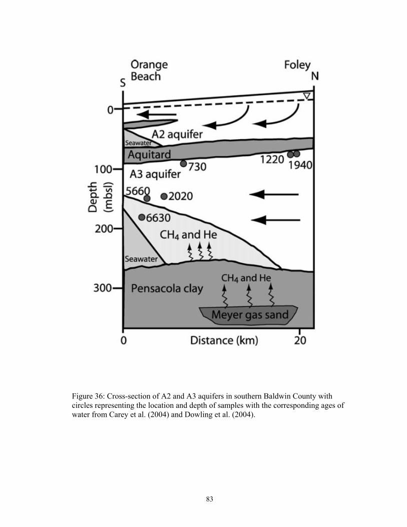
Figure 36: Cross-section of A2 and A3 aquifers in southern Baldwin County with circles representing the location and depth of samples with the corresponding ages of water from Carey et al. (2004) and Dowling et al. (2004).

83

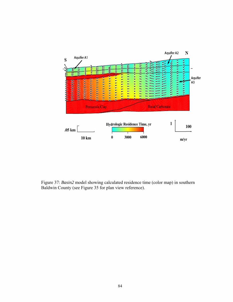
Figure 37: Basin2 model showing calculated residence time (color map) in southern Baldwin County (see Figure 35 for plan view reference).

84

Figure 38: Plot of hydrologic residence time in the A3 aquifer vs. distance.

85

CONCLUSIONS

The mixing that is taking place within the Weeks Bay and Wolf Bay

watersheds strongly impacts the water chemistry and also the methylation of mercury

especially in Weeks Bay. The mixing of seawater, freshwater, and groundwater in

Weeks Bay provides desired geochemical conditions (i.e. warm, low pH and low

salinity) that are necessary for methylation. Surface water in both bays are Na-Cl

type. Wolf Bay has a higher salinity (closer to seawater) that prohibits the favorable

conditions to promote methylation of mercury. The oxygen and hydrogen isotope data

suggest that the chemistry and quality of surface waters of river, creeks, and bays are

affected by evaporation, meteoric recharge, groundwater discharge, and mixing with

seawater. The stable isotope signatures of groundwater fall close to the LMWL,

which indicate minimum evaporation prior to surface discharge. Fish River water

and Weeks Bay water show enrichment of 18O and 2H relative to groundwater,

indicating that they undergo greater evaporation or mixing with isotopically heavier

seawater. Wolf Bay water is enriched in heavy 18 2O and H with respect to those in

Weeks Bay, this and its higher salinity reflects less freshwater inputs and greater

proportion of seawater mixed in the bay. Geochemical analysis suggests that, most

major ions (Na+ 2+, Ca , Mg2+ - -2, Br , etc.), with the exception of SO4 , exhibit

conservative behavior during water mixing in Weeks Bay but most exhibit a more

non-conservative behavior in Wolf Bay. Along with physical mixing and

evaporation, biochemical processes such as sulfate reduction due to bacteria may be

at work in the Weeks Bay watershed as indicated by non-conservative depletion of

86

-2SO4 . It is known that bacterial sulfate reduction is the critical first step for Hg

methylation and bioaccumulation.

The intrusion of seawater into Wolf Bay and Weeks Bay creates a front of

high salinity, high pH water that penetrates below low pH, low-conductivity

freshwater. Along this wedge interface, water at different depths exhibit difference in

water chemistry. The higher discharge of low pH, low-salinity surface water (i.e.,

Fish River) into Weeks Bay may contribute vital conditions that promote the

methylation of mercury. By contrast, salinity in Wolf Bay may be too high for the

methylation to take place. The most rapid changes in water chemistry occur at the

mouth of Wolf Creek flowing into Wolf Bay and in Weeks Bay at the mouth of the

Fish River. The mixing of several waters of different chemical characteristics creates

a favorable environment (i.e., the presence of higher temperature, low pH, and low-

salinity waters) where methylation may occur and cause the spread of mercury

contamination throughout the watershed via bioaccumulation in Weeks Bay but not

Wolf Bay. Low DO and ORP values observed in this mixing zone suggest active

microbial processes that are an important factor in initializing Hg methylation in

Weeks Bay near the mouth of the Fish River, but Wolf Bay has higher DO values in

this mixing zone. Our results imply that Hg biotransformation is strongly influenced

by hydrochemical conditions in coastal watersheds.

87

The most likely source for mercury contamination found in the southern

Baldwin County watersheds is from atmospheric deposition. By examining the

precipitation data from the USGS and mercury deposition data from the MDN show

that an increase in precipitation results in an increase mercury deposition in the

watersheds.

The geophysical surveys conducted on Dauphin Island and Orange Beach

yielded mixed results. On Dauphin Island the electrical resistivity survey had

readings that ranged from highly resistive (unsaturated layers) to low resistive, which

possibly indicating saltwater in the shallow subsurface. The results from the survey

conducted in Orange Beach indicated that the shallow subsurface is comprised of

highly resistant unsaturated layers and not likely to be contaminated by shallow

saltwater. The freshwater-saltwater interface in this area turned out to be deeper than

anticpated. A longer survey length would be needed in order to locate the depth of

the freshwater-saltwater interface.

Regional scale groundwater flow models were developed in a cross section

extending from the northern recharge areas (near Bay Minette) to the Gulf Coast.

The model predicted two flow regimes in major aquifer zones. A local flow regime is

present in Aquifer A2 due to local variations in topography and water table

undulations. In the deeper Aquifer A3, a regional flow regime dominates in which

flow directions are more consistent (i.e., from north to south) and controlled by the

net topographic slope. Groundwater discharges southwards into the coastal estuaries

88

(e.g., Wolf and Weeks bays) and Gulf of Mexico. Calculated groundwater flow

velocities in major aquifers range from a few to tens of meters per year. The model

calculated that groundwater residence time of major aquifers ranges from 0 near the

recharge area to about 7000 years near the Gulf Coast along a 70 km flow path. The

calculated groundwater residence time is consistent with 14 4C and He ages measured

by Carey et al. (2004).

89

REFERENCES

Advanced Geosciences Inc., 2002, Instruction manual for EarthImager 2D, version 2.2.0, resistivity and IP inversion software: Austin, Texas, 134p.

Alabama Water Watch, 2007, Citizen Volunteer Water Monitoring on Alabama’s

Coast - Wolf Bay. Alley, W.M., 1999, Sustainability of Ground-Water Resources, USGS Circular 1186,

79p. Alley, W.M., Healy, R.W., LaBaugh, J.W., Reilly, T.E., 2002, Flow and storage in groundwater systems, Science Vol 296, number 5575, 1985-1990 pp. Al-Jahar, M., Davidson, S., Linhoff, B., Rempe, D., Sharp, J., 2007, Variations in the freshwater/saltwater System on North Padre Island, Texas: free convection or Ghyben-herzberg lens? Paper No. 174-21. Barlow, P.M., 2003, Groundwater in freshwater/saltwater environments of the

Atlantic Coast, United States Geological Survey Circular 1262. Baeyens, W., C. Meuleman, B. Muhaya, and M. Leermakers, 1998, Behaviour and Speciation of Mercury in the Scheldt Estuary (Water, Sediments and Benthic Organisms): Hydrobiologia, v. 366, p. 63-79. Bethke, C.M., Lee, M.-K., and Park, J., 2003, A Guide to Use Basin2 Software

Package, Release 5.0, http://www.geology.uiuc.edu/~bethke/pdf/Basin2UsersGuide.pdf , 20 p.

Carey, A.E., Dowling, C.B., and Poreda, R.J., 2004, Alabama Gulf Coast

groundwaters: 4He and 14C as groundwater dating tools, Geology, 32, p. 289-292.

Celo, V., D. R. S. Lean, and S. L. Scott, 2006, Abiotic Methylation of Mercury in the Aquatic Environment: Science of the Total Environment, v. 368, p. 126-137. Chandler, R.V., Gillett, B., and DeJarnette, S., 1996, Hydrogeologic and water-use

data for southern Baldwin County, Alabama, Geological Survey of Alabama Circular 199, 124 pp.

Chandler, R.V., Moore, J.D., and Gillett, B., 1985, Groundwater chemistry and salt-water encroachment, southern Baldwin County, Alabama, Geol. Survey of Alabama Bulletin 126, 166 pp.

Craig, H., 1966. Isotopic composition and origin of the Red Sea and Salton Sea

geothermal brines. Science 154, 1544–1548.

90

De Breuk, W., De Moor, G., 1969. The water table aquifer in the eastern coastal area of Belgium. Bull. Assoc. Sci. Hydro. 14, p. 137-155. Dowling, C.B., Poreda, R.J., Hunt, A.G., and Carey, A.E., 2004, Ground water discharge and nitrate flux to the Gulf of Mexico, Ground Water, 42, 401-417. Drever, J. I., 1997, The Geochemistry of natural waters, Surface and Groundwater Environments: Upper Saddle River, New Jersey, Prentice Hall. Fetter, C.W., 2001, Applied Hydrogeology, 4th ed., Prentice Hall, New Jersey. Flanzenbaum, J., 1986. Evaluation of saltwater intrusion into the Coastal Aquifer of

Southern Virginia, M.S. Thesis, University of Virginia, 141 pp. Goodell, H.G., 1986. A study of saltwater intrusion into the surface aquifer and the

underlying of Yorktown Aquifer of Coastal Virginia. Final Report to Virginia Environmental Endowment Richmond, VA, 14 pp.

Kim, E., Mason, R.P., Porter, E.T., and Soulen, H.L., 2004, The effect of

resuspension on the fate of total mercury and methylmercury in a shallow estuarine ecosystem: a mesocosm study, Marine Geochem., 86, 121-137.

King, J. K., S. M. Harmon, T. T. Fu, and J. B. Gladden, 2002, Mercury Removal,

Methylmercury Formation, and Sulfate-Reducing Bacteri in Wetland Mesocosms: Chemosphere, v. 46, p. 859-870.

Lee, M.-K., Griffin, J., Saunders, J.A., Wang, Y., Jean, J., 2007, Reactive transport of

trace elements and isotopes in Alabama coastal plain aquifers, Journal of Geophysical Research, 112, G02026, doi:10.1029/2006JG000238.

Leermakers, M., Galletti, S., De Galan, S., Brion, N., Baeyens, W., 2001, Mercury in

the southern North Sea and Scheldt estuary, Marine Chemistry, 75, p. 229-248. Nowroozi, A.A., Horrocks, S.B., Henderson, P., 1999, Saltwater intrusion into the freshwater aquifer in the eastern shore of Virginia: a reconnaissance electrical resistivity survey, Journal of Applied Geophysics, 42, p. 1-22. Marimuthu, S., 2005, Interaction between Surface Water and Groundwater in a

Coastal Wetland System: Ph.D. Thesis, University of Western Australia.

Mason, R.P., Fitzgerald, W.F., and Morel, F.M.M., 1994, the biogeochemical cycling of elemental mercury: Anthropogenic influences, Geochim. Cosmochim. Acta, 58, 3191-3198. Mason, R.P., Lawson, N.M., Lawrence, A.L., Leaner, J.J., Lee, J.G., and Sheu, G.,

1999, Mercury in the Chesapeake Bay, Marine Chemistry, 65, p. 77-96.

91

Mehrotra, A. S., A. J. Horne, and D. L. Sedlak, 2003, Reduction of Net Mercury Methylation by Iron in Desulfobulbus Propionicus Cultures: Implications fo Engineered Wetlands: Environmental Science and Technology, v. 37, p. 3018-3023.

Monrreal, R. H., 2007, Hydrology and water chemistry in Weeks Bay, Alabama:

Implications of mercury bioaccumalation. M.S. Thesis, Auburn University. 65 pp.

Murgulet, D., Tick, G., 2008, The extent of saltwater intrusion in southern Baldwin

County, Alabama, Environmental Geology, v. 55, number 6, p. 1235-1245. Penny, E. and M.-K. Lee, and C. Morton, 2003, Groundwater and microbial processes of Alabama coastal plain aquifers: Water Resources Research, v. 39, p. 1320-

1346. Raymond, D.E., and C.W. Copeland, Selected columnar sections for the Coastal

Plain, Appalachian Plateaus, Interior Low Plateaus, and Valley and Ridge Provinces in Alabama, Geol. Sur. Alabama Atlas Ser., 20, 43 p., 1987.

Reed, P.C., 1971, Geologic map of Baldwin County, Alabama, Geological Survey

Special Map 94:5. Robinson, J., Moreland, R., and Clark, A., 1996, Groundwater resources data for

Baldwin County, Alabama, U.S. Geological Survey Open File Report 96-487. Sabot, M.A., 1975, Vertical electrical resistivity sounding locate groundwater

resources: a feasibility study. Virginia Polytechnical Institute, Water Resources Bulletin 73, 63 pp.

Sakr, S.A., 1999, Validity of a sharp interface model in a confined coastal aquifer,

Hydrogeology Journal, Vol 7 number 2, 155-160 pp. Source Water Assessment Program for Groundwater Systems, Baseline Assessment

Report 2002 for Dauphin Island Water and Sewer Authority’s Public Water Supply Wells prepared by O’Donnell and Associates, Inc., October 2002.

Source Water Protection Areas Delineation and Potential Contaminant Sources

Inventory, Orange Beach North Well Field prepared by Goodwyn, Mills and Caywood Environmental Consultants, Inc., November 1, 2000.

Swarzenski, P., Kruse, S., Reich, C. and Swarzenski, W., 2007, Multi-Channel

resistivity investigations of the freshwater/saltwater interface: a new tool to study an old problem.

92

Ullrich, S. M., T. W. Tanton, and S. A. Abdrashitova, 2001, Mercury in the Aquatic Environment: A Review of Factors Affecting Methylation: Critical Reviews in Environmental Science and Technology, v. 31, p. 241-293.

Wellhead Protection Area Delineation and Potential Contaminant Source Survey

Report, prepared by Layne Geosciences, Inc., November 14, 1997. Zohdy, A.A.R., Martin, P., Bisdorf, R.J., 1993, A study of seawater intrusion using

direct-current soundings in the southeastern part of Oxnard Plain, California. Open-File Report 93-524, U.S.G.S., 139 pp.

93