1

Interacting Regime Shifts in Ecosystems: Implication for Early Warnings 1 W.A. Brock1 and S.R. Carpenter2,3 2

3 A Manuscript for the ‘Concepts and Synthesis’ section of Ecological Monographs 4

5 October 2009 5 6

1Department of Economics 7 University of Wisconsin 8 Madison, Wisconsin 53706 9 10 2Center for Limnology 11 University of Wisconsin 12 Madison, Wisconsin 53706 13 14 3corresponding author. email: srcarpen@wisc.edu 15 16 17 18 19 20 21

2

Abstract. Big ecological changes often involve regime shifts in which a critical threshold is 22 crossed. Thresholds are often difficult to measure and transgressions of thresholds come as 23 surprises. If a critical threshold is approached gradually, however, there are early warnings of the 24 impending regime shift. Autocorrelation approaches 1 from below, variance and skewness 25 increase, and variance spectra shift to lower frequencies. Here we focus on variance, an indicator 26 easily computed from monitoring data. 27 28 There are two distinct sources of increased variance near a critical threshold. One is the 29 amplification of small shocks that occurs as the squared eigenvalue approaches 1 from below. 30 This source, called squealing, is well-studied. The second source of variance, called flickering, is 31 brief excursions between attractors. Flickering has rarely been analyzed in the literature. 32 Analysis presented here accounts for both sources of variance. 33 34 Complex systems exhibit many kinds of thresholds. The case of a single threshold may 35 not fully account for the changes in variance that may occur in systems subject to multiple 36 thresholds. Interacting thresholds may muffle or magnify variance near critical thresholds. 37 Whether muffling or magnification occurs, and the size of the effect, depends on the product of 38 the feedback between the state variables times the correlation of these variables’ responses to 39 environmental shocks. If this product is positive, magnification of the variance will occur. If the 40 product is negative, muffling or magnification can occur depending on the relative magnitudes of 41 these and other effects. 42 43 Simulation studies using a lake food web model suggest that muffling may sometimes 44 interfere with detection of early warning signals of regime shifts. However, more important 45 effects of muffling and magnification may come from their effect on flickering, when random 46 shocks trigger a state change in a system with low resilience. Muffling decreases the likelihood 47 that a random shock will trigger a regime shift. Magnification has the opposite effect. 48 Magnification is most likely when feedbacks are positive and state variables have positively 49 correlated responses to environmental shocks. These results help delimit the conditions when 50 regime shifts are more likely to cascade through complex systems. 51 52 Key words: Alternative stable states, critical transition, early warning, lakes, regime shift, 53 trophic cascade, variance 54

3

INTRODUCTION 55 56 Scientists and managers are increasingly concerned with responses of complex systems to 57 multiple interacting shocks. Recent massive shifts in energy, food and financial markets, and 58 consequences for pollutant emissions and land use, illustrate the connectedness of diverse sectors 59 at the global scale. Linked global changes due to accelerating human activity are creating novel 60 challenges for institutions concerned with managing climate, human health, ecosystem services 61 and the economy (Walker et al. 2009). Connected regime shifts raise the possibility of cascading 62 breakdowns in multiple services with consequences for human well-being. 63 64

Some changes in complex systems are big, persistent, and difficult for managers to 65 reverse (Holling 1973, Scheffer et al. 2001, Walker and Meyers 2004, Scheffer 2009). The 66 generic term 'regime shift' represents this diverse class of big changes (Carpenter 2003, Scheffer 67 and Carpenter 2003, Scheffer and Jeppesen 2007). In ecology, many different kinds of regime 68 shifts are known from oceanic ecosystems, lakes, spatial dynamics of vegetation, drylands 69 subject to desertification, rangelands subject to degradation, and others (Scheffer 2009). 70 Mechanisms of ecological regime shifts are equally diversified. Examples include feedbacks 71 between vegetation and the atmosphere (Foley et al. 2003, Narisma et al. 2007), soil (Rietkerk et 72 al. 2004) or fire (Peters et al. 2004); biogeochemical feedbacks (Carpenter 2003); and complex 73 interactions in food webs (Scheffer 1997, Jeppesen et al. 1998, Schmitz et al. 2006, Persson et al. 74 2007). 75 76

Regime shifts are hard to predict or anticipate (M.A. 2005). Gradual, incremental change 77 may give the impression that an ecosystem is not capable of extensive change that goes beyond 78 the range of historical experience (Carpenter 2002, 2003). Thresholds for regime shifts are not 79 known with precision. They may move over time, so estimates from one time interval may not 80 apply to another time interval. Probability distributions of thresholds are low and wide, with long 81 tails (Carpenter and Lathrop 2008). Such fat-tailed probability distributions may be common for 82 important environmental parameters and such distributions have important implications for 83 decisions and management (Weitzman 2009). Thus the difficulty of measuring ecosystem 84 thresholds is important for applied as well as basic ecology. 85

86 Recent studies, however, show that some ecosystem variables change before regime 87

shifts in ways that may serve as early warnings (Scheffer et al. 2009). For time series 88 observations of ecosystem state variables such as biomasses or chemical concentrations, standard 89 deviations or variances may increase (Carpenter and Brock 2006), variance may shift to lower 90 frequencies in the variance spectrum (Kleinen et al. 2003, Carpenter et al. 2008, Biggs et al. 91 2009, Contamin and Ellison 2009), skewness may increase (Guttal and Jayaprakash 2008) and 92 return rates in response to disturbance may decrease (van Nes and Scheffer 2007) in advance of a 93 regime shift. If monitoring is in place to measure such signals, and managers are able to act 94 swiftly to change key drivers, then catastrophic changes may sometimes be averted (Biggs et al. 95 2009, Contamin and Ellison 2009). 96

97 So far, most theory for early warnings has considered situations in which an ecosystem is 98 subject to a single kind of regime shift. Such systems gradually approach a critical transition as a 99 driving variable changes slowly (Scheffer et al. 2009). But many interactions within ecosystems 100

4

are capable of producing instabilities of various kinds (Ives and Carpenter 2007, Scheffer 2009). 101 It is easy to imagine situations in which a given ecosystem is subject to multiple kinds of regime 102 shifts. Moreover these regime shifts may be connected through other kinds of ecological 103 interactions. If the individual regime shifts are weakly connected, or widely separated in time, 104 then interactions among regime shifts may have negligible effects on early warning indicators. In 105 some cases, however, proximity to one regime shift may affect the resilience of another regime 106 shift in the same ecosystem. It is not clear whether such interactions will increase or decrease the 107 strength of the early warning signal. 108 109 This paper takes first steps toward understanding how interacting regime shifts may 110 affect early warning signals. We focus here on variance which is easily measured using 111 monitoring data from a wide variety of ecosystems. The paper begins with a motivating example 112 of lake ecosystems which may be subject to two or more kinds of regime shifts. Next we make 113 an important distinction between two sources of variance near critical transition points: squealing 114 which is an amplification of variance as the critical point is approached, and flickering which is 115 transient excursions between alternate basins of attraction. The main section of the paper then 116 derives conditions for decreasing (muffling) or increasing (magnifying) variance through the 117 interaction of two critical transitions. We then study the response of variance to the interactions 118 of two distinct but linked critical transitions in a lake food web. We conclude that the role of 119 muffling or magnification in flickering may have important effects on regime shifts induced by 120 random shocks. 121 122

MULTIPLE TRANSITIONS IN TROPHIC CASCADES 123 124

Even though ecosystems are subject to many kinds of critical transitions (Scheffer 2009), 125 most (though not all) studies of critical transitions in ecology have attempted to isolate one 126 particular transition for analysis. Perhaps this is because field study of critical transitions is quite 127 difficult in ecology, so it is simpler to focus on one transition at a time (Carpenter 2003, Scheffer 128 and Carpenter 2003, Petraitis and Latham 1999). Yet it is likely that any given ecosystem could 129 potentially undergo many distinct critical transitions. If two different critical transitions are 130 linked in some way, then observed time series of system behavior could bear the signature of 131 both transitions. 132

133 As a specific example, we address cascading changes in lake ecosystems which are well-134

studied in the context of critical transitions (Carpenter 2003, Carpenter et al. 2008, Scheffer et al. 135 2000). A large body of field studies and models suggest that big changes in food webs of lakes 136 may involve more than one critical transition. Several examples involve interactions of benthic 137 and open-water subsystems, or littoral and pelagic sub-systems (Scheffer 2009). Here we 138 consider two distinct but linked critical transitions that involve fish and zooplankton (Fig. 1) 139 140

Theory and experiments show that massive shifts in fish populations cascade to 141 phytoplankton, thereby changing primary production and a host of associated ecosystem 142 processes (Carpenter and Kitchell 1993). Such big changes in the fish community can result from 143 a trophic triangle (Ursin 1982) involving adults and juveniles of the apex predator interacting 144 with smaller-bodied species of fish. 145

146

5

A trophic triangle involving largemouth bass and golden shiners is embedded in Fig. 1 147 (gray boxes). This triangle is dominated by the apex predator if adult biomass is large enough to 148 suppress populations of the smaller-bodied fish species, or by the smaller-bodied fishes if 149 mortality is high for adult apex predators. High mortality can be inflicted by fishing, resulting in 150 a type of alternate states called “compensation-depensation” by Walters and Kitchell (2001). 151 Theory suggests that (1) plausible models for the fish shift can be represented as a critical 152 transition, (2) various time-series statistics such as autoregression coefficients, variance and its 153 multivariate analogs, skewness and variance power spectra change in predictable ways prior to 154 the critical transition, and (3) these statistical signals are transmitted downward through the food 155 chain to zooplankton and phytoplankton (Carpenter et al. 2008). 156

157 A second type of critical transition can occur in the plankton (Fig. 1, hatched boxes). The 158

trophic interactions among carnivorous invertebrates such as the phantom midge (Chaoborus), 159 large-bodied herbivorous crustaceans such as Daphnia, and small-bodied herbivorous 160 crustaceans such as Bosmina or small diaptomid copepods can produce sharp transitions in 161 grazer body size, community composition, morphology and behavior (Dodson 1974, Neill 1975, 162 Hall et al. 1976, Kerfoot 1980). If planktivory by fishes is low, mortality of phantom midges and 163 large-bodied Daphnia is low. While small Daphnia can be consumed by phantom midges, large-164 bodied Daphnia have life-history and morphology adaptations that enable them to reach high 165 abundance even when phantom midges are abundant (Hall et al. 1976, Kerfoot 1980). Small-166 bodied grazers are, however, vulnerable to phantom midges and can be suppressed by phantom 167 midge predation. If phantom midge abundance is reduced by fish predation, small-bodied grazers 168 become dominant. Thus, as planktivory by fishes is adjusted upward or downward there are 169 strong shifts in body size of herbivorous crustaceans, mediated by phantom midge or other 170 carnivorous invertebrates. These shifts resemble critical transitions. They are linked to, but 171 distinct from, the critical transitions studied in piscivore-planktivore systems. 172

173 What happens if the critical points for these transitions occur at different points in time, 174

one before the other? Or what if they coincide? One could imagine several different possibilities. 175 The statistical signals of the different transitions might fall in sequence, leading to a cascade of 176 increasingly intense signals. Or the statistical signals may blur together, perhaps obscuring any 177 early warning signal. This is the general issue that we wish to explore. 178 179

SQUEALING AND FLICKERING 180 181 As an entry point to the analysis, we first address changes in variance during critical 182 transitions in discrete-time stochastic dynamical systems with multiple equilibria. An example is 183 sketched in Fig. 2A. In this section of the paper, we discuss two different sources of variance that 184 increase as the curve of Fig. 2A rises with respect to the diagonal line. First, variance may 185 increase as the slope of the curve approaches 1 from below (Fig. 2B) (Carpenter and Brock 186 2006). This source of increased variance, which we will call “squealing”, has been analyzed 187 thoroughly in the literature (Biggs et al. 2009, Scheffer et al. 2009). Second, variance may 188 increase because of brief excursions from one attractor to the other (Fig. 2C). In Fig. 2C, starting 189 at the low equilibrium, a large shock can move the system past the unstable equilibrium into the 190 basin of attraction of the upper equilibrium. This kind of variance, which we call “flickering”, 191 can occur only if the stochastic envelope around the curve includes all three equilibria. 192

6

Flickering may increase variance over many time steps if the system moves back and forth 193 between the stable attractors over a period of time. In this section of the paper, we make the 194 notion of flickering more precise and establish a framework to study squealing and flickering in 195 systems where multiple critical transitions can interact. 196 197

We introduce some ideas that will be used throughout the paper using a one dimensional 198 stochastic dynamical system in discrete time (t), 199 200 (1) 1 1 1 2 2 1 1( ) ( ( )) 1[ ], given, 1, 2,...t t t t cx a s t s t x be x x x t 201

202 Symbol definitions are collected in Table 1. Here the dynamics of the state variable x involve the 203 conditional mean a , two slow variables s1 and s2, a shock process bet+1, and a switching process 204

1[ ]t cx x . We explain these in turn. 205

206 The slowly-changing variables follow two functions, 1 2( ), ( )s z s z which are differentiable 207

in z. They are written as ( ), 1, 2i is t i to emphasize that as t increases by one step, the 208

quantities ( )i is t increase by a very small amount since the functions are differentiable and the 209

0, 1,2i i are a very small positive numbers. 210

211 Shocks { }te follow a second order stationary sequence of random variables, each with 212

mean zero and variance 2e . We assume the processes 1 2{ },{ }t te e are independently and 213

identically distributed with zero mean and unit variance. 214 215

Switching is represented by the indicator function 1[.]. This function is one if the event in 216 [.] occurs and is zero otherwise. Note that a predator-prey interaction in which x2 preys on x1 217 could be represented by (1) if 12 and 12b terms in the right side of equation (1) were negative so 218

a positive shock or a jump up in 2tx decreases 1tx . 219

220 The switching terms in equation (1) are closely related to sigmoid functions used in many 221

ecological models. Switch terms can be smoothed as follows. Note that as q tends to infinity the 222 function, 0( , ) : / ( )q q qg x q x x x tends to an “up” switch at 0x . I.e. as q , 223

224 (2) 0 0 0 0( , ) : / ( ) ( , ) 0, , 1/ 2, , 1,q q qg x q x x x g x x x x x x x 225

226 If we slightly modify the definition of 01[ ]x x to 227

228 (3) *

0 0 0 01 [ ] : 0, , 1/ 2, , 1,x x x x x x x x , 229

230 then we see that we can approximate a switching function as closely as we wish with a smooth 231 approximating function. Peterson et al. (2003) used such switching models to investigate 232 questions of policy choice and learning for ecosystems subject to critical transitions. 233 234

7

Squealing can occur in equation (1) as a slow variable moves the curve upward so that 235 the lower equilibrium approaches the threshold, or downward so that the upper equilibrium 236 approaches the threshold. When squealing occurs, ρ2 approaches one from below which 237 increases the steady state variance 2 2 2var( ) / (1 )tb e . This point is discussed in detail in 238

the appendix of Biggs et al. (2009). 239 240 Using this framework we can highlight the distinction between squealing and flickering 241 by simplifying to a model where squealing cannot occur, but flickering can occur. We will fix 242 the value of ρ in equation (1) for all t, where 0 1 . We will bound the shocks so that { }te is 243

a second order stationary stochastic process of uncorrelated binary random variables, each with 244 mean zero and taking the value -1 with probability ½ and +1 with probability ½. The result is 245 246 (4) 1 1 1[ ]t t t t cx a x be x x 247

248 We portray this system setting the threshold point 2cx in Fig. 3. The system has two stable 249

equilibria and an unstable equilibrium (Fig. 3A). Squealing cannot occur because the slope ρ is 250 constant. However, flickering can occur. Indeed, flickering can occur even if the slope ρ is zero 251 (Fig. 3B). For certain values of the parameter 0a it is possible for the shocks to move the 252 system between the two positive equilibria (Fig. 2A). This highlights the contrast between early 253 warning signs that are based on a slow variable increasing 2 towards one from below which 254

increases the steady state variance 2 2 2var( ) / (1 )tb e and early warning signals that are 255

produced by flickering from one attractor to another. 256 257

MUFFLERS AND MEGAPHONES 258 259 As gradual change in a driving variable moves a one-dimensional system toward a 260 threshold (Fig. 2), the approach to the threshold will be announced by growing variance caused 261 by squealing and flickering. Will the same early warnings occur in a more complex system with 262 multiple thresholds? The answer is not obvious. Interactions in the more complex system could 263 act as a muffler or as a megaphone, respectively decreasing or increasing the noise. In this 264 section of the paper we analyze the conditions for muffling or magnifying the variance as a 265 multidimensional system approaches a critical transition. 266 267 To make the question more precise, we compare the variance of a one-dimensional 268 system approaching a threshold in isolation to the variance that occurs when the same critical 269 transition is embedded in a more complex system. For clarity of analysis we use a two-270 dimensional switching model that builds on the ideas in the preceding section. In a subsequent 271 section of the paper we turn to a case study of an example that uses continuous nonlinear 272 functions instead of switches. 273 274

8

A Switching Model for Interacting Attractors 275 276 Throughout this section of the paper, we will consider a two-dimensional switching 277 system that serves as a stark representation of an ecosystem where critical transitions can occur 278 in each of two subsystems. The model is given by 279 280 (5.a) 1, 1 1 11 1 12 2 11 1, 1 12 2, 1 11 1 1 12 2 21[ ] 1[ ]t t t t t t c t cx a x x b e b e x x x x 281

282 (5.b) 283

2, 1 2 21 1 22 2 21 1, 1 22 2, 1 21 1 1 22 2 2 2 3 23 3 31[ ] 1[ ] ( ) 1[ ]t t t t t t c t c t t cx a x x b e b e x x x x S x x x 284

285 We will assume that the autoregression parameters ρ are functions of very slowly-moving 286 variables as in equation (1), but we will not write them as functions in order to simplify notation. 287 We also assume that 3tx operates on a much slower time scale than 1 2and t tx x . Moreover we 288

assume the slow variable 3tx is deterministic since its time scale is much slower than the 289

simultaneous time scales that we are assuming for the dynamics of the phytoplankton biomass 290 and zooplankton biomass. Here { }, 1,2ite i are second order stationary stochastic processes 291

which are uncorrelated over time and where each has mean zero and unit variance. The ei,t are 292 shocks to species 1 2 and x x . The b parameters are impact factors of these shocks on each 293

species. While our analysis focuses on the case of upward switches (or jumps) in both 1 2and t tx x 294

as well as 3tx , equations (3) are general. 295

296 It is useful to write (3) in matrix form 297

298 (5.c) 1 1 1[ ]t t t t c tx a x be x x f 299

300 where now , , , , , , ,s c s tx a b x e f are 2x1 column vector, 2x1 column vector, 2x2 matrix, 2x2 301

matrix, 2x2 matrix, 2x1 column vector, 2x1 column vector, and 2x1 column vector, respectively. 302 Note that the elements of the 2x1 vectors and 2x2 matrices are defined to be compatible with 303 (5.a,b) above. 304 305

An important assumption is evident from the considering the very simple case where the 306 2x2 matrix is the zero matrix and the forcing term tf is zero. Then using the lag operator L 307

we have 308 309 (6a) 1 1 1( ) ( ) ( ) ( )t t tx I L a e I a I L e 310

311 We assume that the matrix series 312 313 (6b) 2 ...I 314 315

9

converges in order that the stationary distribution of (6a) exist and be well defined. Hence we 316 assume that the norm || || 1 for a matrix norm ||.|| such that || || (|| ||)(|| ||)AB A B for any two 317 matrices A,B. This will ensure that the matrix series in (6b) converges. 318 319

Calculations and concepts below will also consider the dynamics of , i=1,2itx ignoring 320

the interactions with the rest of the system. 321 322 (6c) 1 1 1(1 ) ( ) (1 ) (1 ) , i=1,2.it ii i ii it ii i ii ii itx L a e a L e 323

324 We may use (6) to compute h-step-ahead forecast errors as well as the long run variance-325 covariance matrix of the vector x. Linear expressions like (6) are used in constructing early 326 warning signals in nonlinear systems via linearizations of nonlinear stochastic dynamical 327 systems around deterministic steady states (called “small noise” expansions; Biggs et al. 2009, 328 Williams 2004). 329 330

Conditions for Muffling or Magnifying Variance 331 332

We define muffling and magnifying in terms of the relative magnitudes of two variances: 333 the variance of x1 as if it existed alone, separate from the interacting system, versus the variance 334 of x1 when it is part of the interacting system. If the first variance (x1 alone) exceeds the second 335 variance (x1 embedded in the whole system), then the system interactions muffle signals from x1. 336 If the first variance is less than the second variance then the signals are magnified by the full 337 system of interactions. 338

339 In this sub-section of the paper, we will restrict analysis to a system cannot flicker 340

(because there are no switches) but it can squeal because of the very slow change in ρ. That is 341 we set = 0. We use this simplified system to introduce some basic features of muffling and 342 magnifying for the stationary long-term variance and the one-step ahead forecast variance. In the 343 next subsection, we return to the more general case where 0 and consider the h-step ahead 344 forecast errors in a system that can both flicker and squeal. 345

346 First we consider the whole system. We compute the variance-covariance matrix of the 347

stationary distribution of the vector tx from (6a) to obtain 348

349

(7a) '

0

' 'n nt t e

n

E x x b b

350

351 where, '

t tE x x denotes the 2x2 variance covariance matrix of x computed w.r.t. the stationary 352

distribution computed from (6a). Here ':e t tEe e the variance-covariance matrix of the et which 353

is independent of t by stationarity. The upper prime on a matrix denotes transpose. Equation 354 (7a) is computed using the assumption, ' 0, for all , ,t sEe e s t s t 355

356

10

Second, we use (6c) to compare the variance of the stationary distribution of 1x alone as 357

if it were not part of the 2x2 system and compare that variance with the variance of 1x taking 358

into account the interactions of x1 with 2x in the 2x2 system in which 1x is embedded. The right 359

side of the inequality (7b) below is the variance of 1x alone. It is computed using (6c). The left 360

side of the inequality (7b) below is the variance of 1x taking into account the interaction of 2x 361

with 1x . It is computed using (6a). 362

363 Third, in order to locate sufficient conditions for the interactions with the rest of the 364

system to muffle (vs magnify) the variance of 1x , we locate sufficient conditions such that the 365

inequality 366 367

(7b) 1 1,

2 211 11 11 11

0

: [ ' ' ] ( ) / (1 )n nx x e e

n

b b b

368

369 holds. In expression (7b) the ‘<’ condition is for muffling the variance, the ‘(>)’ condition is for 370 magnifying the variance. Inequality (7b) says the variance of 1x taking into account interactions 371

with the rest of the 2x2 system is less (greater) than the “stand alone” variance computed using 372 (6c). We explain the notation in (7). First, for any matrix A, [ ]ijA denotes the (i,j)’th element of 373

the matrix A. Second, 1 1,x x

denotes the variance of x1 computed at the stationary distribution, 374

i.e. 1 1,x x

is the (1,1) element of the 2x2 matrix in (7a). At the risk of repeating, we assumed 375

' '0, ,m n n n eEe e m n Ee e to compute (7a). As noted above we need to assume that the norm 376

|| || 1 for a matrix norm ||.|| such that || || (|| ||)(|| ||)AB A B for any two matrices A,B so that 377 the series in (7) converges. 378 379

There is an equivalent expression for (7a) which is useful for reducing the location of 380 sufficient conditions for (7b) to a manageable task. Using (6) we compute 381 382 (7c) ' ' ' , Q:= 't t t t eE x x E x x Q b b 383

384 On the surface it does not look like (7c) is helpful since it is a matrix fixed point equation. But 385 symmetry of the moment matrix ': t tM E x x implies (7c) is just a system of three equations in 386

three unknowns, 11 12 21 22, ,M M M M . Hence the system (7c) may be expressed as a linear 387

system of three equations and three unknowns. This system can be solved using Cramer’s Rule. 388 We will use this method below to locate sufficient conditions on (7c) for muffling and 389 magnifying where these concepts are introduced in the definition below. 390 391 Definition 1 (Long Run Signal Muffling (Magnifying)): We say that the long run signal on 1x is 392

muffled (magnified) if (7b) (the reverse of (7b)) holds. A similar definition holds for 2x . 393

394

11

The meaning of “muffled” and “magnified” is intuitive. On the one hand, if the 1x -part of the 395

system were independent of the rest of the system except for a variable that pushed the 1x -396

dynamics towards a local bifurcation then the early warning signal would be increasing 1x -397

variance as the local bifurcation is approached because the absolute value of the slope of the 1x -398

linearization is approaching one. That local 1x -variance is the right side of inequality (7b). On 399

the other hand, the left side of inequality (7b) is the local variance of 1x taking into account the 400

interactions with the rest of the system when 1x is not independent of the rest of the system. 401

402 Definition 2 (1-step-ahead-forecast error muffling (magnifying)): We say that the 1-step-ahead 403 forecast error is muffled (magnified) if 404 405 (8) 2 2

11 11 ,11 11 11 ,11[ '] , ([ '] )e e e eb b b b b b 406

407 A bit of matrix algebra shows that (8) holds iff 408 409 (9) 12 11 12, 22, 12 11 12, 22,| | 2 | | / , ( | | 2 | | / )e e e eb b b b 410

411 For example, the “<” part of inequality (9) holds when the shocks to 1x and 2x have a large 412

enough absolute value of correlation and the standard deviation of the shock to 1x is large 413

enough relative to the direct impact of a shock to 2x to 1x . 414

415 We are now ready to consider the case of h-step ahead forecast errors. We may compute 416

these objects using (6a). We obtain for the h-step-ahead forecast error vector, 417 418 (10) 2 1

| 1 2 ( 1)... ht h t h t t h t h t h t h hx x be be be be 419

420 The variance covariance matrix is given by 421 422 (11) 1 1

| |{( )( ) '} ' ' ' ... ' 'h ht h t h t t h t h t e e eE x x x x b b b b b b 423

424 Note that (11) converges to (7a) as h tends to infinity provided that || || 1 . 425 426

Expression (11) exposes two interesting points. First, if the 2x2 matrix is diagonal the 427 condition for muffling of h-step-ahead forecast variance is the same as for one-step ahead 428 forecast variance, i.e. expression (8). This is so because the -specific terms cancel off both 429 sides of the inequality. This will not hold for the general case where is not a diagonal matrix. 430 Second, as || || approaches one from below, the right side of expression (11) will tend to 431 become larger and the right side of equation (11) will tend to become infinite as h tends to 432 infinity. This latter statement is made rigorous in the Appendix to Biggs et al. (2009). 433 434

12

Variance of h-step Ahead Forecast Errors With Flickering and Squealing 435 436

We now have the background material needed for the case that is perhaps most useful for 437 analyzing real-world ecosystems – finite-horizon h-step ahead forecast errors where both 438 flickering and squealing are possible. We now assume that the the 2x2 matrix is nonzero. 439 Switches and therefore flickering are possible. To compute h-step-ahead forecast errors, analysis 440 must therefore take into account the possibility of switches between attractors. 441 442

Let us assume that the forcing term 0, for all ttf in order to break the analysis down 443

into manageable units. We begin by looking at conditions for muffling due to offsetting jumps 444 (or drops) to occur for 2-step-ahead forecast errors. This extra effect can not occur for 1-step-445 ahead forecast errors since 1 1| 1t t t tx x be , i.e. we need at least two periods to pick up the 446

effect of jumps. Compute, using (3.c), to obtain 447 448 (12) 2 2 2| 2 1 1 1 |: (1[ ] 1[ ] )t t t t t t t c t c tfe x x be be x x x x 449

450 where 451 452 (13) 1 | 11[ ] : {1[ ] | }t c t t c tx x E x x x . 453

454 We compute 455 456 (14) ' ' ' '

2 2 1 1 1 1 1 1{ } ' ' ' ( ) ' ( ) ' ' ( ) 't t t e e t t t t t t t t tE fe fe b b b b b E e z E z e b E z z 457

458 where {.}: {.} |t tE E x and 1 1 1 |: (1[ ] 1[ ] )t t c t c tz x x x x . We see right away that the first, 459

second, and last terms of (14) are positive (in the matrix sense of being positive definite 460 matrices). Therefore they can only magnify the signal. However, terms three and four could be 461 positive or negative. If they are negative and sufficiently large, they could cause muffling of the 462 signal. 463 464

Equation (14) is crucial for understanding h-step-ahead variance. Because it is a 465 complicated expression, we will exposit it by the following steps. First we study (14) for the 466 scalar case. This task is carried out in equations (15)-(20) below. Second, we study (14) for a 467 two variable case where the feedback from 2x to 1x is zero, i.e. 21 210 , i.e. the ρ matrix is 468

triangular. Equation (21) describes this system. This case is motivated by the trophic cascade 469 example which is analyzed later in the paper. Even with this simplification, it is useful to begin 470 by assuming the matrix 0 in order to focus on flickering by excluding squealing. This task 471 is carried out in equations (22)-(27) below. In the case of h-step-ahead forecast errors the 472 strength of squealing as the leading eigenvalue of the matrix approaches one is very limited 473 for small h. This signal, in contrast to flickering, only becomes strong for large h. Hence we 474 will study the case of nonzero only for the case h . This case is studied in equations (28)-475 (31) below. 476 477

13

We compute (14) for the scalar case. Since we are interested in warning signals of a 478 critical transition, we compute (14) under the assumption that 1t cx x , i.e. no critical transition 479

has yet occurred. We first focus on the case where cx is crossed from below due to gradual 480

increase in a slow driving variable, which we call an “upcrossing.” Then we discuss the case 481 where cx is crossed from above, which we call a “downcrossing”. 482

483 We obtain, for both cases of upcrossing and downcrossing, 484

485 (15) 2 2 2 2 2 2 2 2

2 1 1 1{ } 2 ( ) ( )t t e e t t t t tE fe b b b E e z E z 486

487 where we now compute each of the last two individual terms under the assumption that no 488 critical transition has yet occurred and for an upcrossing. We compute, 489 490 (16) 1 | 1 11[ ] : {1[ ] | } {1[ ] | } 1 (( ) / )t c t t c t t t c t e c tx x E x x x E a x be x x F x a x b , 491

492 where 1( ) : Pr{ }e tF w e w is the cumulative distribution function of the shock and is 493

independent of t by stationarity. We compute the conditional covariance variance of z with the 494 shock and the conditional variance of z. We obtain 495 496

(17) 1 1 1 1 1 |

( )/

{ (1[ ] 1[ ] )} 0c t

t t t t t t c t c t e

e x a x b

E e z E e x x x x edF

497

498

where the positive right side of (17) follows follows from 0e

e

edF and the fact that the right 499

side is integrating over larger values of e, 500 501 (18) 2 2

1 1 1 | 1 1 |[(1[ ] 1[ ] )] { [(1[ ])}{(1 1[ ] )])}t t t t c t c t t t c t t c tE z E x x x x E x x E x x . 502

. 503 Using (16) to compute the terms in {.} in (18) we obtain 504 505 (19) 2

1 ( (( ) / ))(1 (( ) / ))t t e c t e c tE z F x a x b F x a x b . 506

507 We collect our computations and end up with a full expression for the right side of equation (15). 508 509

(20a)

2 2 2 2 2 22

( )/

2

{ } 2 ( )

( (( ) / ))(1 (( ) / ))

c t

t t e e e

e x a x b

e c t e c t

E fe b b b edF

F x a x b F x a x b

510

511 Formula (20a) shows a contrast between the potential power of an early warning signal 512

based upon slowly increasing (squealing) in contrast to an early warning signal based upon 513

1tx passing through a critical transition where there is a jump (flickering). Note that, in the case 514

where the product of the autoregression parameter ρ, shock impact b, and switch magnitude is 515

14

non-negative ( 0b ) the covariance between the shock and z does not muffle the signal. 516

Note also that the jump signal is strongest when 1/ 2eF because that is when the last term on 517

the right side of equation (20) is maximum at the value 2 / 4 . That is, the signal is maximum 518 strength at the median. If the median is zero (a natural median for a mean zero random variable) 519 then we have the signal is at maximum strength when t ca x x . Note that when 0 the 520

signal is at maximum strength when ca x . Hence if there is a slow variable S that moves ( )a S 521

gradually closer to :c ca x we see from (20) that the signal from the variance of 2-step-ahead 522

forecast errors of impending critical transition gets stronger when 0b . This flickering 523 signal is independent of any signal based upon increasing variance from the movement of the 524 autocorrelation coefficient towards unity from below. 525 526

Now consider the case of a down crossing of cx where the value of x falls by . We 527

obtain, (letting mine denote the lower bound of the set of e’s with positive probability, which may 528

be ), 529 530

(20b) min

( )/2 2 2 2 2 2

2

2

{ } 2 ( )( )

( (( ) / ))(1 (( ) / ))

c tx a x b

t t e e e

e

e c t e c t

E fe b b b edF

F x a x b F x a x b

531

532 Notice that even if 0b the second to the last term now muffles the signal when a jump is 533

negative. This is so because the term, min

( )/

0c tx a x b

e

e

edF

. This latter conclusion follows from 534

the mean of “e” being zero and the latter integral being over the lower values of “e”. 535 536

Triangular ρ Matrix 537 538 In trophic cascades, the impact of a top predator to certain prey is stronger than the 539 impact of these prey on the predator. Such a system can persist if the predator has multiple food 540 sources as shown in the example of Fig. 1. We represent such a system by a triangular ρ matrix 541 and a triangular matrix in which one feedback is negligible: 542 543 (21.a) 1, 1 1 11 1 12 2 11 1, 1 12 2, 1 11 1 1 12 2 21[ ] 1[ ]t t t t t t c t cx a x x b e b e x x x x 544

545 (21.b) 2, 1 2 22 2 22 2, 1 22 2 2 21[ ]t t t t c tx a x b e x x f 546

547 (21.c) 2 2 3 23 3 3: ( ) 1[ ]t t t cf S x x x 548

549 In this system the feedback from 1tx to 2tx is so weak that we approximate it by zero. We shall 550

start analysis by restricting ourselves to upcrossings and to a situation where no upcrossings have 551

15

yet occurred. Notice also that a drop can occur in the 2tf term in (21.b) due, perhaps to a jump 552

in the biomass of the predator that feeds on 2x . 553

554 Zero ρ Matrix: An Informative Special Case 555

556 Recall that (14) exhibits a decomposition of forces for muffling (magnifying) into three 557

components: (i) shocks (through the term 'eb b ), (ii) dynamics (propagated through the matrix 558

), and (iii) jumps and drops (captured in the term, '1 1( ) 't t tE z z ). The complexity of (14) 559

reflects the interactions amongst these three forces. In this subsection of the paper we obtain 560 useful analytical results by simplifying the analysis of equation (14) by assuming the matrix 561

0 so we can evaluate muffling or magnifying in a system subject to flickering but not 562 squealing. It makes sense to focus on the case 0 for smaller h’s, e.g. h=2, because the 563 strength of the squealing signal, i.e. the increase in variance as the leading eigenvalue of the 564 matrix approaches one, is muted unless h is quite large. We have, from (14), for the case 565

where the matrix 0 and the forcing term for the dynamics of 2tx , i.e., 3 0tf , 566

567 (22) ' '

2 2 1 1{ } ' ( ) 't t t e t t tE fe fe b b E z z 568

569 We wish to locate sufficient conditions for muffling (magnifying) to occur in (22), i.e., 570 571 (23) ' 2 2 '

11 1 1 11 11 11 11 1 1 11[ '] [ ( ) '] ( ) [( )]e t t t e t t tb b E z z b E z z 572

573 It is convenient for the computations below to put , 1 1 1, 1 2 2, 1: , i=1,2i t i t i tn b e b e . Note that 574

: ' 'n eEnn b b are independent of date t by stationarity. Using this notation for the shocks, 575

we have, 576 577 (24) , 1 , 1 , 1 |1[ ] 1[ ], 1[ ] 1 ( ), i=1,2

ii t ic i i t ic i t ic t n ic ix x a n x x x F x a . 578

579 We now compute the elements of '

1 1( )t t tE z z , where , 1, 2inF i denotes the cumulative 580

distribution functions of the shocks. Shorten the notation by putting '1 1 :t t t zE z z which is 581

independent of date t by stationarity. We obtain, by computation, 582 583

(25) ,

2,12 1, 1 1 1 2, 1 2 2 1

(1 ( )) ( ),

Pr{ , , } (1 ( ))

i i

i

z ii n ic i n ic i

z t c t c i n ic i

F x a F x a

n x a and n x a F x a

584

585 Of course when the n’s are independent ,12 0z . 586

587 Since we have already investigated sufficient conditions for 2

11 11 11[ '] ( ) e eb b b in 588

material surrounding equation (8), we turn here to investigating sufficient conditions for 589 590

16

(26) ' 2 '1 1 11 11 1 1 11[ ( ) '] ( ) [( )]t t t t t tE z z E z z . 591

592 Computing, and using the shorter notation above, we obtain that (26) holds, iff, 593 594 (27) 2 2 2

11 ,11 12 11 ,12 12 ,22 11 ,112 ( )z z z z 595

596 Later in the paper we use simulation to investigate cases where r12 is negative, zero or 597

positive, where 1/2 1/212 ,12 ,11 ,22: / ( )n n nr is the correlation coefficient. Since zero correlation is not 598

the same as independence we proxy 12 0r with independence which implies ,12z =0 (which is 599

not implied by zero correlation because of the nonlinearity of the indicator function). We note 600 that for ,12z =0, expression (27) shows that the signal is always magnified by the possibility of 601

jumps (drops) over and beyond magnification (muffling) induced by dependence in the shocks. 602 Since 2x preys on 1x in the example below, the “natural” case is 12 0 . We then have two 603

subcases, ,12 ,120, 0n n . For the case 12 ,120, 0n , (27) shows that the signal is always 604

magnified. One suspects that this is a “natural” case since one suspects that the n’s are 605 negatively correlated since 2x is predator and 1x is prey. Negatively correlated n’s make it 606

easier for ,12 0n in (25). This can be seen intuitively by assuming 2, 1 1, 1t tn n , then it is 607

easy for 1, 1 1 1 2, 1 2 2Pr{ , , }t c t cn x a and n x a to be zero and hence, ,12 0n . 608

609 Nonzero Triangular ρ Matrix 610

611 We return now to the case where the 2x2 matrix is not the 2x2 zero matrix. We assume 612

that ρ is a function of variables that change very slowly, so that squealing and flickering can both 613 occur. We shall assume that the matrix norm of is less than one as well as other regularity 614

conditions, e.g. the variance matrices ,e f are finite, so the steady state distribution of tx 615

exists. 616 617

We compute the steady state variance covariance matrix of equation (5.c) under the 618 assumption that 1{ }te is an Independent and Identically Distributed process across time with 619

mean vector zero and finite variance matrix, e . First we observe that the steady state mean 620

vector for x is given by 621 622 (28) 1[ ] : 1t c tx a x E x x E f a x f 623

624 Let y x x . Then 625 626 (29) ' ( ') ' 'eE yy E yy b b R 627

628 where the notation (“R” for “residual”), 1, 2,,R R denote the matrices containing the other terms. 629

Recall that muffling (magnifying) of variable , 1, 2ix i occurs when 630

17

631 (30) 2 2 2 2

, 1, , 1,< (>) [ '] [ ( ') '] [ '] [ ]i ii i ii e ii ii ii ii e ii iiE y E y b R E yy E yy b b R 632

633 where 634 635 (31) 1, 2,( )( ) ' {(1[ ] 1)(1[ ] 1) '} 't t t c t cR E f f f f E x x x x R 636

637 Equation (30) compares the steady state variance of each ix when all connections with the rest of 638

the system are set equal to zero with the steady state variance of each ix when the connections 639

are taken into account. A lot of complexity is embedded in the notation of expression (30). We 640 observe that muffling (magnifying) comes from three sources: (i) interactions from the 641 nondiagonal terms of the matrix, (ii) interactions from the nondiagonal terms of the b and e 642

matrices, (iii) interactions from the nondiagonal terms of the 1,R matrix. The 1,R matrix is 643

complicated because it captures the variance matrices of , 1[ ] 1t t cf f x x as well as the 644

cross interactions among the terms, , 1[ ] 1, t t c tf f x x y y all computed at the steady state 645

distribution. 646 647

We observe from (30) that if all matrices in (28) are diagonal and e is diagonal, then 648

(30) collapses to two independent scalar systems and no issues of muffling (magnifying) can 649 arise. Second, we observe that if 2

ii approaches one from below, we should expect the steady 650

state variance of ix to become infinite. Third, when we consider the variance matrices of 651

, and, 1[ ] 1t t cf f x x , we see that muffling (magnifying) is impacted by interactions within 652

the vector of outside forcings as well as interactions within the vector of potential jumps (drops). 653 The vector of outside forcings of the dynamics between 1 2and x x is due to forces like fish 654

predation, habitat modification, etc. Fourth, muffling (magnifying) is also impacted by the cross 655 terms in the matrix 2,R in equation (31). Summing up, we see that muffling (magnifying) can 656

occur due to (i) interactions in squealing (due to non zero cross terms in the matrix), (ii) 657 interactions in flickering (due to nonzero cross terms in the matrix and the 658

{(1[ ] 1)(1[ ] 1) '}t c t cE x x x x matrix), (iii) interactions in outside forcing (due to nonzero 659

cross terms in the {( )( ) '}t tE f f f f matrix), (iv) interactions in the shocks (due to nonzero 660

cross terms in the b matrix and the e matrix), (v) interactions in cross product terms (due to 661

nonzero cross terms in the 2,R matrix). In view of this complexity, it is difficult to say more 662

using analytical methods. Below we turn to simulations. 663 664

AN ECOSYSTEM EXAMPLE 665 666

We now turn to a more realistic model of an ecosystem subject to two different but 667 coupled critical transitions. We focus on two critical transitions that can occur in lake food webs, 668 compensation-depensation in the fish community and the shift between large-bodied and small-669 bodied herbivorous crustaceans in the zooplankton (Fig. 1). We assume that gradual increase in 670

18

fishing of the piscivore is the exogenous slow driver. Increasing fishing mortality of adult 671 piscivores will eventually release the planktivores to surge in biomass as they cross a critical 672 transition. At some level of planktivory by fishes, large-bodied zooplankton will suffer high 673 mortality and collapse in biomass to be replaced by small-bodied zooplankton. But it is not at all 674 clear whether the threshold for the zooplankton shift occurs before, at the same time, or after the 675 threshold for the planktivorous fishes. Here we abstract the complex interactions of Fig. 1 and 676 consider only the planktivorous fishes and large-bodied herbivorous crustacean zooplankton as 677 indicator variables for the two critical transitions. The fish dynamics are assumed to provide the 678 slower-moving driver for the plankton dynamics. We ask how the dynamics are affected by 679 variance due to the two critical transitions that can occur in the system. 680

681 Variance When Two Thresholds Interact 682

683 In this subsection we analyze a generic model for trophic cascades with two critical 684

transitions, in order to derive an amplification index. The value of the amplification index is 685 proportional to the degree of muffling or magnifying conferred by dynamics of the full system. 686 The equation for the amplification index reveals some general features of systems that tend to 687 muffle or magnify variance. The model is 688 689 (32) , 1 , 1exp[ ( ) ], i=1,2i t it i ii i tx x f x b e . 690

691 Symbols for the simulation example are collected in Table 2. In most cases these are consistent 692 with the first part of the paper. The exception is f which now stands for the rate function not an 693 external forcing. 694 695

We will linearize the model around an equilibrium that is gradually being destabilized by 696 slow increase in fishing mortality of the piscivore (Carpenter et al. 2008). This is the equilibrium 697 with low biomass of planktivorous fish and high biomass of large-bodied herbivorous 698 zooplankton. Let , 1, 2ix i denote the components of a positive deterministic steady vector of 699

(32) when the e’s are set equal to zero, i.e. 1 2( , ) 0, i=1,2if x x . 700

Let : , i=1,2it it iy x x , define ( )

:i

i iy

df yf

dx , and expand the system (32) in a Taylor 701

series around the 2x1 vector x to obtain 702 703 (33a)

1 21, 1 1 1 1 1 1 2 1 11 1, 1 11 1, 1(1 ) ( , )t x t x t t t ty x f y x f y x b e o y b e 704

705 (33b)

1 22, 1 2 2 1 2 2 2 2 22 2, 1 22 2, 1(1 ) ( , )t x t x t t t ty x f y x f y x b e o y b e 706

707 where , 1( , ), 1, 2t ii i to y b e i are functions that go to zero faster than the norm of ty plus the 708

absolute value of , 1ii i tb e i=1,2 go to zero. Hence the shocks as well as the deviations must be 709

“small” in order for the linear part of equation (33) to be a good approximation. Furthermore we 710 assume both eigenvalues of the linearization matrix in equation (33) are inside the unit circle of 711 the complex plane. This assumption implies that the steady state vector x is locally 712

19

asymptotically stable as well as the matrix equation (35) below having a unique solution (Biggs 713 et al. (2009, Appendix)). 714 715

We write the linear part of (33) in matrix form as 716 717 (34) 1 1t t ty y n , 718

719 where the elements of the matrix and the vector n come from (33). We analyze the triangular 720 case where ρ21 = 0. This corresponds to the lake trophic cascade example where the fishes switch 721 to other prey when large-bodied zooplankton are scarce. 722 723

By (7c) we obtain the following matrix equation for the steady state moment matrix, 724 725 (35) ' ' 't t t t nE y y E y y 726

727 where , 1 1 1, 1 2 2, 1: , i=1,2i t i t i tn b e b e , and : 'n Enn . The shocks {e} are assumed to be mean 728

zero second order stationary processes so, therefore, the impacts {n} are also second order 729 stationary processes. To simplify notation, no subscripts “t” appear on the moment matrix Enn’. 730 731 Recall that symmetry of the steady state moment matrix ': t tM E y y implies (35) is just a 732

system of three equations in three unknowns, 11 12 21 22, ,M M M M . Hence the system (35) may 733

be expressed as a linear system of three equations and three unknowns. When the off diagonal 734 terms ,

jixf i j are set equal to zero, we have 735

736 (36) 2

, , / (1 )ii diag n ii iiM . 737

738 Here ,n ii denotes the (i,i) element of the 2x2 moment matrix n which was defined above. 739

740 It is clear from (36) that if the system is diagonal and there is a slow variable that is 741

gradually pushing 2ii up to one from below then the steady state variance ,ii diagM goes to 742

infinity. This is an early warning signal of a bifurcation where an eigenvalue of a linearization 743 passes through +1. We are interested in locating sufficient conditions on ,n such that muffling 744 (magnifying) occur, 745 746 (37) , ,, ( )ii ii diag ii ii diagM M M M 747

748 We may write a system of three linear equations in the three unknowns 11 12 21 22, ,M M M M 749

from (35) and solve it using Cramer’s Rule or, equivalently by using the inverse of the associated 750 3x3 matrix of weights on the three M’s from (35). An alternative approach using Kronecker 751 products is discussed by Ives et al. (2003). Here we apply Cramer’s rule to solve for 11M and 752

obtain the condition (38) for the “triangular” case where 21 0 , 753

20

754 (38) 2 1/2 1/2 2

12 22 12 11 12 ,11 ,22 22 ,22 12 22 22 112 [ (1 ) ] / (1 ) <0 (>0)n n n nr 755

756 The left side of (38) is an amplification index. It tells us whether variance is decreased or 757 increased by the full set of interactions. If r12 and ρ12 are the same sign, then the amplification 758 index must be positive and variance must be magnified by the interactions. If r12 and ρ12 are 759 opposite in sign, then the amplification index could be negative if the first term and last term of 760 the amplification index are sufficiently small. If the amplification index is negative then the 761 variance is decreased by the interaction. To see why the outcome depends on the signs of r12 and 762 ρ12, remember that the diagonal ρ terms are less than unit magnitude and positive. Therefore the 763 amplification index must be positive if r12ρ12 is positive. If r12ρ12 is negative, then the second 764 term of the amplification index is negative and if it is sufficiently large in magnitude then the 765 amplification index will be negative. 766 767

Threshold Interactions in a Simulated Food Web 768 769

We simulated the dynamics of planktivorous fish (x2) and large-bodied zooplankton 770 grazers (x1) using 771 772

(39)( )

, 1 ,

, , , , , , , , ,( ) ( )( )( )

if xi t i t

i t i i t l i i t c i i t u i i t i t

x x e

f x c x a x a x a s N

773

774 Equilibria are the a’s with subscripts denoting the lower stable root (l), intermediate unstable 775 root or critical transition point (c), and upper stable root (u). The parameter ci scales the per-776 time-step growth of state variable i. The noise Ni,t is independently and identically distributed 777 multivariate normal with mean zero and variance-covariance matrix Σ. Shocks to the state 778 variables are correlated within each time step but uncorrelated across time. The si,t are slowly-779 changing variables where s2 represents changes to the fish community caused by slow changes in 780 fishing mortality of an apex predator. The fish variable x2 changes more slowly than the 781 zooplankton variable x1. Planktivore generation times are two or more years, whereas 782 zooplankton generation times are about one to three weeks. Therefore it is plausible that x2 can 783 act as a slow variable for the dynamics of x1. The interaction is represented by s1,t which not a 784 constant, but changes over time as a function of x2,t. Specifically we assumed 785 786 (40) 1, 2, ,t l ts kx 787

788 where 2, ,l tx is the lower stable equilibrium of planktivores given the current value of s2,t. The 789

sign of k can be positive or negative depending on the zooplankton group represented by x1. 790 Large-bodied herbivorous zooplankton have a negative relationship to x2, whereas small-bodied 791 herbivorous zooplankton have a positive relationship to x2. 792 793 Simulation studies examined muffling or magnification of variance for both negative and 794 positive values of k (Fig. 4). In each case, we compared four sets of simulations: high and low 795 levels of resilience for both planktivorous fish and zooplankton. We define resilience of a stable 796

21

point as the distance (in units of the state variable) of a stable point from the unstable threshold 797 (Holling 1973). The different levels of resilience were achieved by adjusting s2 and k. In each 798 case, we solved for equilibria and computed eigenvalues for the linearization of the deterministic 799 skeleton of the model to confirm that there were three real roots, that the upper and lower roots 800 were stable, and that the middle root was unstable. In each of these four sets of simulations, we 801 computed variance for x1 alone (uncoupled from x2) and for the coupled system with three 802 different values for the correlation coefficient of shocks: r12 = -0.9, 0 or +0.9. All other 803 parameter values were fixed for all simulations (Table 2). Parameter values were selected to 804 yield alternate state biomasses and thresholds similar to those obtained by Carpenter et al. (2008) 805 who fitted a model to field data from ecosystem experiments. We computed the amplification 806 index (left side of expression 2.7) and variance of both state variables. The variance was 807 computed for 1000 time steps near equilibrium using programs written in R (http://www.r-808 project.org/) by S.R.C. 809 810

Negative Effect of x2 on x1 811 812 Here we analyze the situation where planktivorous fish are near their lower stable point 813 and large-bodied zooplankton are near their higher stable point (Fig 4 A, C). When fishing 814 mortality of piscivores increases, planktivorous fish biomass increases. In the model, s2,t 815 increases thereby moving the lower stable point of x2 closer to the unstable threshold of x2. Thus 816 resilience, in the sense of Holling (1973), of the lower stable point of x2 decreases. The increase 817 in 2, ,l tx causes s1,t to decrease, thereby decreasing the resilience of the upper stable point of x1 818

(i.e. this upper stable point moves closer to the unstable threshold). 819 820 When k is negative, then ρ12 is negative because 12 1kx , from expression (33a). 821

Therefore we expect an inverse relationship between the amplification factor and r12, the 822 correlation of the shocks, from expression (38) 823 824 First we examined the case when shock variances (diagonal elements of Σ) are equal. 825 With equal shock variances and negative ρ12, the amplification factor was positive for this 826 particular set of parameter values. 827 828 When resilience of both state variables was relatively high, variance was relatively low 829 and the amplification factor was near zero (Fig. 5A). The contrast is striking with the case in 830 which resilience of both state variables was relatively low (Fig. 5D). The amplification factor is 831 positive, indicating that variance is magnified by the dynamics of the interacting system. There is 832 a slight tendency for the amplification factor to decline as the correlation of shocks increases. 833 The variance of x1 alone (uncoupled from x2) is less than the variance observed for the coupled 834 system at any value of the correlation coefficient for shocks. 835 836

Variance also increased notably when resilience of zooplankton was decreased to a low 837 value while resilience of planktivores remained high (Fig. 5B). The amplification factor shows 838 that the system dynamics magnify the signal of the nearby threshold in zooplankton. The 839 amplification factor and the variance of x1 decline as the correlation of shocks increases. This 840 highlights the potential impact of correlated shocks on early warnings of critical transitions. 841

842

22

The case where planktivore resilience is low and zooplankton resilience is high shows 843 strongly muted variance of zooplankton (Fig. 5C). Indeed, variance of zooplankton is not 844 discernibly different from the case where both variables have high resilience (Fig. 5A). In 845 contrast, variance of planktivorous fish increased markedly in Fig. 5C compared to Fig. 5A. This 846 substantial increase in variance of planktivores was not expressed in the zooplankton. The 847 amplification factor was small. This example shows that the early warning of a nearby transition 848 in a predator may not be expressed in the variance of the prey. 849 850 We now turn to a case where the shock variance to zooplankton, Σ11, is 104 larger than 851 shock variance to planktivorous fishes, Σ22 (Table 2). For the parameter values of this simulation, 852 the amplification factor is positive for negative r12, and negative for positive r12. 853 854 When resilience of both state variables was relatively high, variance was relatively low 855 and the amplification factor was near zero (Fig. 6A). The outcome was different when resilience 856 of both state variables was relatively low (Fig. 6D). The amplification factor is positive for 857 negative r12, and negative for positive r12. The variance of x1 and x2 is larger when both variables 858 have low resilience (Fig. 6D) than when the variables are farther away from their thresholds (Fig. 859 6A). 860 861

Variance of zooplankton, x1, also increased when its resilience was decreased to a low 862 value while resilience of planktivores remained high (Fig. 6B). The amplification factor varies 863 inversely with r12. However, the magnitude of muffling or magnifying is not large. Increased 864 variance of x1 signals the close approach of that variable to its threshold. 865

866 The case where planktivore (x2) resilience is low and zooplankton (x1) resilience is high 867

evoked low variance of zooplankton (Fig. 6C). Variance of zooplankton is not different from the 868 case where both variables have high resilience (Fig. 6A). In contrast, variance of planktivorous 869 fish increased. As in the case of equal variances, the early warning of a nearby transition in a 870 predator may not be expressed in the variance of the prey. 871

872 Positive Effect of x2 on x1 873

874 To study responses with positive k, we analyzed the situation where planktivorous fish 875 are near their lower stable point and zooplankton are also near their lower stable point (Fig. 4 876 B,D). Instead of representing large-bodied zooplankton, x1 now represents small-bodied 877 zooplankton near their lower stable point. Biomass of small-bodied zooplankton is inversely 878 related to that of large-bodied zooplankton through the interactions described in Fig. 1. When 879 fishing mortality of piscivores increases, planktivorous fish biomass increases. In the model, s2,t 880 increases thereby moving the lower stable point of x2 closer to the unstable threshold of x2. Thus 881 resilienceof the lower stable point of x2 decreases. With positive k, the increase in 2, ,l tx causes 882

s1,t to increase, thereby decreasing the resilience of the lower stable point of x1 (i.e. this lower 883 stable point moves closer to the unstable threshold). 884 885

With k positive, we examined case where the shock variance to zooplankton, Σ11, is 104 886 larger than shock variance to planktivorous fishes, Σ22. In this situation the amplification factor 887 changes in the same direction as r12: negative for negative r12, and positive for positive r12. 888

23

889 Results were rather similar to the cases described above (Fig. 7). The same three patterns 890

were evident. (1) Variance of each state variable increased as its resilience decreased. (2) The 891 amplification index responded as expected. However strong effects of muffling or magnification 892 were not evident. (3) In the case when planktivorous fish had low resilience but small-bodied 893 zooplankton had high resilience (Fig. 7C), neither the amplification index nor the zooplankton 894 variance changed appreciably, in comparison with the case where both state variables have high 895 resilience (i.e. compare Fig. 7A with Fig. 7C). 896 897

DISCUSSION 898 899 In ecosystems subject to critical transitions, the approach to a regime shift can be 900 announced by increase of the autocorrelation coefficient toward 1, increased variance or 901 skewness, or shift of the variance spectrum toward lower frequencies (Kleinen et al. 2003, 902 Carpenter and Brock 2006, Guttal and Jayaprakash 2008, van Nes and Scheffer 2007, Contamin 903 and Ellison 2009, Scheffer et al. 2009). These indicators may serve as diagnostics of critical 904 transitions in long-term observed data (Dakos et al. 2008). In management, the indicators may 905 reveal incipient regime shifts before they occur, allowing managers some time to take action to 906 avert unwanted regime shifts (Scheffer et al. 2009). Such applications raise important questions 907 about appropriate time series filters for data, statistical sensitivity of indicators, the amount of 908 time available to take effective action, and design of responsive institutions (Kleinen et al. 2003, 909 Carpenter and Brock 2006, Contamin and Ellison 2009, Biggs et al. 2009). This paper turns to a 910 different issue of interpreting variance shifts in ecosystems subject to multiple critical transitions. 911 912

If the ecosystem is subject to two different but linked critical transitions, early warning 913 indicators may behave in more complex or even counter-intuitive ways. This paper has 914 investigated the interactions of regime shifts by focusing on variance in discrete-time models. 915 We address discrete time because ecological time series are sampled discretely, and discrete time 916 is a reasonable way to model many ecological processes. We address variance because it is 917 perhaps the simplest indicator to measure in field data, due to the availability of efficient 918 estimators for small sample sizes. 919 920

As a discrete-time system approaches a critical point (specifically as the squared 921 eigenvalue approaches one from below) the variance will increase from two distinct sources. The 922 first source is the shift of the steady state variance 2 2 2var( ) / (1 )tb e toward infinity as the 923

squared autocorrelation ρ2 approaches one from below. Theory and examples for this source of 924 variance, or squealing, have been discussed elsewhere (Brock and Carpenter 2006, Brock et al. 925 2008, Carpenter and Brock 2006, Biggs et al. 2009, Scheffer et al. 2009). 926

927 The second source of variance, flickering, can occur if the range of the noise is large 928

enough to occasionally push the system across a critical threshold. This shock-driven shift may 929 be temporary, if subsequent shocks move the system back to the original attractor, or persistent if 930 subsequent shocks move the system back to the original attractor. Scheffer et al. (2009) noted the 931 distinction between flickering and squealing but did not pursue the idea in detail. Flickering is 932 more likely to be important in discrete-time models, where it is possible to jump across 933 thresholds, than in continuous time models where dynamics are very slow near thresholds. 934

24

Nonetheless, flickering occurs in a continous-time model of lake dynamics subject to relatively 935 small shocks to nutrient recycling and relatively larger shocks to nutrient input from the 936 watershed (Carpenter and Brock 2006). In the paleoclimate record, transitions between century-937 scale cold and warm periods are marked by rapid transitions between dusty and dust-free 938 conditions, with as many as four such flickers preceding each transition (Taylor et al. 1993). 939 During the transition from anaerobic to aerobic earth, about 2.7 to 2.3 billion years ago, three 940 flickers of oxygenation of the atmosphere seem to have occurred before planetary primary 941 production rates became high enough to maintain an oxygenated atmosphere (Godfrey and 942 Falkowski 2009). 943

944 Ecosystem dynamics can muffle or magnify variance due to a nearby critical transition. 945 The effect of ecosystem dynamics depends on the interaction between the state variables that are 946 subject to critical transitions. For two variables, each subject to a critical transition, the effect on 947 variance depends on the sign of the interaction between the variables (ρ12) multiplied by the sign 948 of the correlation of the response of the variables to environmental shocks (r12). In a predator-949 prey or competitive relationship the sign of the interaction will be negative. Correlation of the 950 response to environmental shocks is less obvious. It is easy to think of cases where both species 951 respond in the same direction to a given shock, as well as cases where species respond oppositely 952 to a given shock. 953 954 If the sign of ρ12r12 is positive, then ecosystem interactions magnify the variance. Such 955 interactions increase the intensity of the early warning of an impending regime shift. For a 956 predator-prey interaction, magnification will occur if the two species have opposite responses to 957 environmental variability. 958 959

If the sign of ρ12r12 is negative, then ecosystem interactions can muffle or magnify the 960 variance, depending on the relative magnitudes of the terms in equation (38). If muffling occurs, 961 the signal of an impending regime shift would be muted, and perhaps prevent an early warning. 962 For a predator-prey interaction, muffling will occur if the two species have respond in the same 963 direction to environmental variability. 964

965 Our findings complement studies of the effect of correlated and autocorrelated 966

environmental noise on linear ecological systems (Ripa and Ives 2003, 2007). Correlated and 967 autocorrelated environmental shocks can have large effects that are not intuitive. For example 968 they can muffle or magnify predator-prey cycles (Ripa and Ives 2003). Because environmental 969 correlations and autocorrelations can muffle or magnify dynamical patterns, underlying 970 phenomena such as predation and competition can become less or more detectable in long-term 971 data (Ripa and Ives 2007). Thus the interaction of environmental noise with ecosystem processes 972 poses profound challenges for inferring ecological interactions from time-series data. 973

974 As our simulations show, ecosystem interactions can suppress the expression of an early 975

warning for an impending regime shift. Early warnings were weakest in cases where predator 976 resilience was low yet prey resilience was high (Figs. 5C, 6C, 7C). This suggests the need for 977 great caution in interpreting early warning signals based on variance. Yet early warning signals 978 were strongly expressed in fishes when their resilience was low, and in zooplankton when their 979 resilience was low. 980

25

981 Other models of lake food webs have demonstrated rather strong transmission of variance 982

(Carpenter 1988) including in situations where variance is generated by an approaching critical 983 transition (Carpenter et al. 2008). In these cases, unlike the present case, a nonlinearity in top 984 predators was linked to a linear food chain. In this paper we consider a food web with two 985 critical transitions. Even though low resilience in a predator increases variance in the predator 986 biomass, this variance is not necessarily transmitted to the prey if the prey resilience is high. 987

988 Another cause of low variance transmission in these simulations is the very small 989

magnitude of the shock variances relative to the resilience of the state variables. Simulations 990 used small shock variances and rather high resilience in order to sample the stationary 991 distribution for long periods of time without causing a regime shift by flickering. In nature, 992 shocks could be larger in relation to resilience, and flickering could lead to much larger changes 993 in variance. Of course such flickering could also trigger a regime shift. 994

995 Nonetheless, our results show that muffling and magnification should be considered in 996

applications of early warnings for ecosystem regime shifts. The magnitude depends in 997 complicated ways on the structure and parameters of the ecosystem model under study. While 998 our analyses suggest the potential importance of muffling and magnification in the dynamics of 999 ecosystems subject to multiple kinds of critical transitions, individual cases may show unique 1000 patterns. 1001

1002 The conditions for muffling versus magnification suggest a straightforward solution for 1003

the dangers of variance muffling in field studies. Measurements should be made for two state 1004 variables, one that has a negative link to the critical transition and one that has a positive link to 1005 the critical transition. The critical transition of planktivorous fishes in our example has a negative 1006 effect on large-bodied herbivores but a positive effect on small-bodied herbivores. Thus large- 1007 and small-bodied herbivores have oppositely-signed values for ρ12. Therefore at least one group 1008 of herbivores will magnify the early warning, provided that the sign of r12 is the same for both 1009 groups of herbivores. As a general rule for ecosystem monitoring, one should plan to measure 1010 variables that are likely to have opposite responses to the regime shifts of interest. 1011

1012 Muffling and magnification have a further important implication for regime shifts, one 1013

that is distinct from their role in early warnings. Flickering may trigger regime shifts. A review 1014 of case studies (Scheffer et al. 2002) argued that many cases of regime shifts in ecosystems were 1015 caused by random shocks to systems with low resilience. Results presented here show that 1016 interactions of different critical transitions in an ecosystem affect the susceptibility of the 1017 ecosystem to regime shifts caused by shocks. Conditions that increase muffling will decrease the 1018 chance of regime shifts caused by shocks. Conversely, conditions that increase magnification 1019 will increase the chance of regime shifts caused by shocks. Therefore, muffling and 1020 magnification must be considered when evaluating the risk that a system will undergo a regime 1021 shift. Expanding linkages among climate, ecosystems, human health and the economy may 1022 increase the frequency of connected global regime shifts in the future (Walker et al. 2009). 1023 Where these are linked by positive feedbacks and have positively correlations to exogenous 1024 shocks there is greater chance of cascading regime shifts. 1025

1026

26

It is likely that many complex systems have the potential for regime shifts (Scheffer 1027 2009). Some kinds of regime shifts are known, even if thresholds are hard to predict, but other 1028 types of regime shifts are as yet unknown. In view of the rich complexities of environmental 1029 systems, it is likely that many links across critical transitions can occur. Scientists attempting to 1030 understand these phenomena are in the early days of a complex and challenging enterprise. 1031 Further development and evaluation of regime shift indicators will require careful system-1032 specific modeling combined with detailed data-based field investigation. 1033 1034

ACKNOWLEDGEMENTS 1035 1036 Tony Ives, Mike Pace and Marten Scheffer provided thoughtful comments on the manuscript. 1037 This work was supported by NSF grants to S.R.C. W.A.B. acknowledges support by NSF and 1038 the Vilas Trust. 1039 1040

LITERATURE CITED 1041 1042 Biggs, R., S.R. Carpenter and W.A. Brock. 2009. Turning back from the brink: Detecting an 1043 impending regime shift in time to avert it. Proceedings of the National Academy of Sciences 1044 106: 826-831. 1045 1046 Brock, W. A. and S. R. Carpenter 2006. Variance as a leading indicator of regime shift in 1047 ecosystem services. Ecology and Society 11 (2): 9. [online] URL: 1048 http://www.ecologyandsociety.org/vol11/iss2/art9/ 1049 1050 Brock, W.A., S.R. Carpenter, and M. Scheffer. 2008. Regime shifts, environmental signals, 1051 uncertainty and policy choice. p. 180-206 in J. Norberg and G. Cumming (eds.), A theoretical 1052 framework for analyzing social-ecological systems. Columbia, NY, USA. 1053 1054 Carpenter, S.R. 2002. Ecological futures: building an ecology of the long now. Ecology 83: 1055 2069-2083. 1056 1057 Carpenter, S.R. 2003. Regime shifts in lake ecosystems: Pattern and variation. Ecology 1058 Institute, Oldendorf/Luhe, Germany. 1059 1060 Carpenter, S.R. and W.A. Brock. 2006. Rising variance: A leading indicator of ecological 1061 transition. Ecology Letters 9: 311-318. 1062 1063 Carpenter, S.R., W.A. Brock, J.J. Cole, J.F. Kitchell and M.L. Pace. 2008. Leading indicators of 1064 trophic cascades. Ecology Letters 11: 128-138. 1065 1066 Carpenter, S.R. and J.F. Kitchell (eds.). 1993. The trophic cascade in lakes. Cambridge 1067 University Press, Cambridge, England. 1068 1069 Carpenter, S.R. and R.C. Lathrop. 2008. Probabilistic estimate of a threshold for eutrophication. 1070 Ecosystems 11: 601-613. 1071 1072

27

Contamin, R. and A.M. Ellison. 2009. Indicators of regime shifts in ecological systems: what do 1073 we need to know and when do we need to know it? Ecological Applications 19: 799-816. 1074 1075 Dakos, V., M. Scheffer, E.H. van Nes, V. Brovkin, V. Petoukhov and H. Held. 2008. Slowing 1076 down as an early warning system for abrupt climate change. Proceedings of the National 1077 Academy of Sciences 105: 14308-14312. 1078 1079 Dodson, S.I. 1974. Zooplankton competition and predation: an experimental test of the size-1080 efficiency hypothesis. Ecology 55: 605-613. 1081 1082 Guttal V, Jayaprakash C. 2008. Changing skewness: an early warning signal of regime shifts in 1083 ecological systems. Ecology Letters 11: 450-460. 1084 1085 Hall, D.J., S.T. Threlkeld, C.W. Burns and P.H. Crowley. 1976. The size-efficiency hypothesis 1086 and the size structure of zooplankton communities. Annual Review of Ecology and Systematics 1087 7: 177-208. 1088 1089 Holling, C.S. 1973. Resilience and stability of ecological systems. Annual Review of Ecology 1090 and Systematics 4: 1-23. 1091 1092 Ives, A.R. and S.R. Carpenter. 2007. Stability and diversity of ecosystems. Science 317: 58-62. 1093 1094 Ives, A.R., B. Dennis, K.L. Cottingham and S.R. Carpenter. 2003. Estimating community 1095 stability and ecological interactions from time-series data. Ecological Monographs 73: 301-330. 1096 1097 Jeppesen, E., M. Sondergaard, M. Sondergaard, and K. Christofferson (eds.) 1998. The 1098 structuring role of submerged macrophytes in lakes. Springer-Verlag, Berlin. 1099 1100 Kerfoot, W.C. 1980. Evolution and ecology of zooplankton communities. University Press of 1101 New England, Hanover, New Hampshire, USA. 1102 1103 Kleinen, T., H. Held, and G. Petschel-Held. 2003. The potential role of spectral properties in 1104 detecting thresholds in the earth system: application to the thermohaline circulation. Ocean 1105 Dynamics 53: 53-63. 1106 1107 MA (Millennium Ecosystem Assessment). 2005. Ecosystems and human well-Being: Our 1108 human planet: Summary for decision makers. Island Press, Washington D.C. 1109 1110 Narisma, G.T., J.A. Foley, R. Licker, and N. Ramankutty. 2007. Abrupt changes in rainfall 1111 during the twentieth century. Geophysical Research Letters 34, L06710, 1112 doi:10.1029/2006GL028628. 1113 1114 Neill, W.E. 1975. Experimental studies of microcrustacean competition, community composition 1115 and efficiency of resource utilization. Ecology 56: 809-826. 1116 1117

28

Persson, L., P.-A. Amundsen, A.M. De Roos, A. Klemetsen, R. Knudsen, and P. Primicerio. 1118 2007. Culling prey promotes predator recovery – alternative states in a whole-lake experiment. 1119 Science, 316: 1743-1746. 1120 1121 Peters, D.P.C., R.A. Pielke Sr., B.T. Bestelmeyer, C.D. Allen, S Munson-McGee, S. and K.M. 1122 Havstad. 2004. Cross-scale interactions, nonlinearities, and forecasting catastrophic events. 1123 Proceedings of the National Academy of Sciences 101: 15130-15135. 1124 1125 Petraitis, P.S. and R.E. Latham. 1999. The importance of scale in testing the origins of 1126 alternative community states. Ecology 80: 429-442. 1127 1128 Rietkerk M., S.C. Dekker, P.C. de Ruiter, and J. van de Koppel. 2004. Self-organized patchiness 1129 and catastrophic shifts in ecosystems. Science 305: 1926-1929. 1130 1131 Ripa, J., and A. R. Ives. 2003. Food web dynamics in correlated and autocorrelated 1132 environments. Theoretical Population Ecology 64:369-384. 1133 1134 Ripa, J., and A. R. Ives. 2007. Interaction assessments in correlated and autocorrelated 1135 environments. In D. A. Vasseur, and K. S. McCann, eds., The impact of 1136 environmental variability on ecological systems. Springer, Dordrecht, Germany. 1137 1138 Scheffer, M. 1997. The ecology of shallow lakes. Chapman and Hall, London. 1139 1140 Scheffer, M. 2009. Critical transitions in nature and society. Princeton University Press, 1141 Princeton, NJ, USA. 1142 1143 Scheffer, M., J. Bascompte, W.A. Brock, V. Brovkin, S.R. Carpenter, V. Dakos, H. Held, E.H. 1144 Van Nes, M. Rietkerk and J. Sugihara. 2009. Early warning signals for critical transitions. Nature 1145 461: 53-59. 1146 1147 Scheffer, M. and S.R. Carpenter. 2003. Catastrophic regime shifts in ecosystems: linking 1148 theory to observation. Trends in Ecology and Evolution 12: 648-656. 1149 1150 Scheffer, M., S. Carpenter, J. Foley, C. Folke and B. Walker. 2001. Catastrophic shifts in 1151 ecosystems. Nature 413: 591-596. 1152 1153 Scheffer, M., Rinaldi, S. and Kuznetsov, Y.A. 2000. The effect of fish on plankton dynamics: a 1154 theoretical analysis. Canadian Journal of Fisheries and Aquatic Sciences 57: 1208-1219. 1155 1156 Schmitz, O.J., E.L. Kalies, and M.G. Booth. 2006. Alternative dynamic regimes and trophic 1157 control of plant succession. Ecosystems 9: 659-672. 1158 1159 Ursin, E. 1982. Stability and variability in the marine ecosystem. Dana 2: 51-65. 1160 1161 van Nes, E. and M. Scheffer. 2007. Slow recovery from perturbations as a generic indicator of a 1162 nearby catastrophic shift. The American Naturalist 169: 738-747. 1163

29

1164 Walker, B. and J.A. Meyers. 2004. Thresholds in ecological and social-ecological systems: A 1165 developing database. Ecology and Society 9(2):3, URL: 1166 http://www.ecologyandsociety.org/vol9/iss2/art3 1167 1168 Walker, B., S. Barrett, S. Polasky, V. Galaz, C. Folke, G. Engstrom, F. Ackerman, K. Arrow, S. 1169 Carpenter, K. Chopra, G. Daily, P. Ehrlich, T. Hughes, N. Kautsky, S. Levin, K-G. Maler, J. 1170 Shogren, J. Vincent, T. Xepapadeas and A. de Zeeuw. 2009. Looming global-scale failures and 1171 missing institutions. Science 325: 1345-1346. 1172 1173 Walters, C. and J.F. Kitchell. 2001. Cultivation/depensation effects on juvenile survival and 1174 recruitment: implications for the theory of fishing. Canadian Journal of Fisheries and Aquatic 1175 Sciences 58: 39-50. 1176 1177 Walters, C.J. and S.J.D. Martell. 2004. Fisheries ecology and management. Princeton 1178 University Press, Princeton, N.J. 1179 1180 Weitzman, M. 2009. On modeling and interpreting the dynamics of catastrophic climate change. 1181 Review of Economics and Statistics 91: 1-19. 1182 1183 Williams, N. 2004. Small noise asymptotics for a stochastic growth model. Journal of Economic 1184 Theory 119(2):271-298. 1185 1186

30

Table 1. Symbols used in the mathematical analysis in this paper. Symbols used in the 1187 simulations are presented in Table 2. 1188 1189 Symbol Definition 1[] Indicator function which is 1 if the event [.] occurs and zero otherwise a conditional mean b effect of a shock E expectation operator e random variable, where {et} is a stationary sequence of random variables, each with

mean zero and variance 2e

Fe(w) cumulative probability distribution of shocks, i.e. 1( ) : Pr{ }e tF w e w

ft exogenous forcing of a system g(x,q) sigmoid function of x with exponent q; 0( , ) : / ( )q q qg x q x x x

L lag operator n shock effect; , 1 1 1, 1 2 2, 1: , i=1,2i t i t i tn b e b e

Q matrix of shocks multiplied by their effects; : 'Q b b

q exponent of a sigmoid function R residual matrices used to analyze the case of h-step-ahead forecast errors when the

autoregression matrix is nonzero and triangular. The R matrix is complicated because it contains the variance of forcing and switching, and all their cross-interactions, all computed at the steady-state distribution.

s a slowly-changing variable or function t time x state variable xc critical transition point (threshold) for a state variable z change in a switching variable over one time step,

i.e. 1 1 1 |: (1[ ] 1[ ] )t t c t c tz x x x x

jump or drop factor in a switching equation ε tiny positive number ρ autoregression coefficient standard deviation Σe variance-covariance matrix of shocks, E(et’et) 1190 1191

31

Table 2. Symbols used to describe the simulations in this paper. Symbols used in the 1192 mathematical analysis are presented in Table 1. 1193 1194 Symbol Definition Numerical Values a equilibrium values for unforced dynamics For x1: 1, 3, 6

For x2: 0.25, 1, 2.5 b effect of a shock c rate coefficient For x1: 0.015

For x2: 0.2 e random variable, where {et} is a stationary sequence of

random variables, each with mean zero and variance 2e

E expectation operator f rate function for state variable i

iyf derivative of a rate function w.r.t. x, evaluated at yi

k effect of x2 on the slow variable that forces x1 scenarios with negative k: -0.01, -0.48, -0.2, or -0.25 scenarios with positive k: 0.06, 0.23, 0.06, or 0.12

M steady-state moment matrix : 't tM E y y

N IID multivariate noise process with variance-covariance matrix Σ

n shock effect; , 1 1 1, 1 2 2, 1: , i=1,2i t i t i tn b e b e

o(.) higher-order terms from a Taylor expansion r12 correlation coefficient of shocks to x1 and x2;

0.5 0.512 12 1,1 2,2: / ( )r

-0.9, 0 or +0.9

s1 slow variable that affects x1 s2 slow variable that forces x2 0 or 0.48, depending on

the scenario x state variable y small deviation of a state variable from equilibrium ρ first-order terms of a Taylor expansion Σ variance-covariance matrix of shocks var(x1) = 10-5; var(x2) =

10-5 or 10-9 as specified; covariance computed from r12

1195

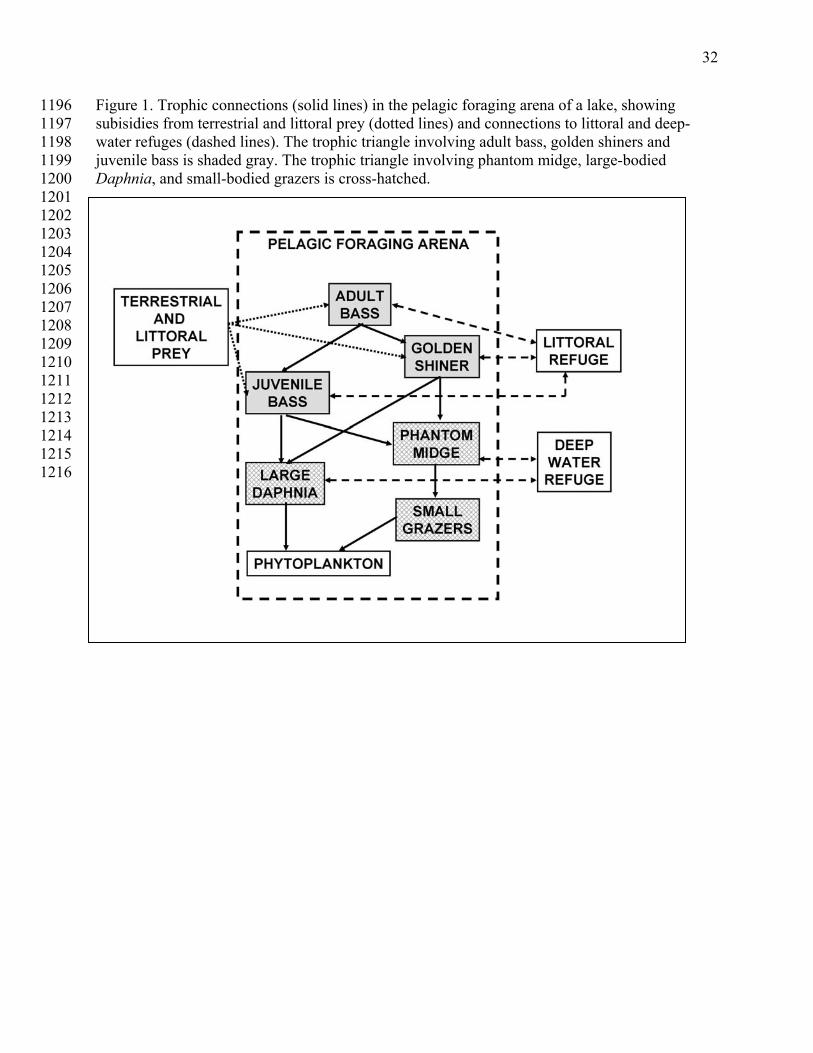
32

Figure 1. Trophic connections (solid lines) in the pelagic foraging arena of a lake, showing 1196 subisidies from terrestrial and littoral prey (dotted lines) and connections to littoral and deep-1197 water refuges (dashed lines). The trophic triangle involving adult bass, golden shiners and 1198 juvenile bass is shaded gray. The trophic triangle involving phantom midge, large-bodied 1199 Daphnia, and small-bodied grazers is cross-hatched. 1200 1201 1202 1203 1204 1205 1206 1207 1208 1209 1210 1211 1212 1213 1214 1215 1216

33

Figure 2. xt+1 versus xt for a system with three equilibria (black curve) showing upper and lower 1217 bounds for the stochastic shocks (gray curves). Dotted line shows xt+1 = xt. The upper and lower 1218 equilibria are stable and the middle equilibrium is an unstable threshold. (A) Base case. (B) The 1219 curve has moved upward a small amount. Variance of xt+1 increases near the lower equilibrium. 1220 This increase, called squealing, is related to the change in slope (eigenvalue) of the curve where 1221 it crosses the diagonal line (see text). (C) The curve has moved upward farther. Flickering – 1222 shocks that move the system across the unstable threshold – can occur. (D) The curve has moved 1223 so far upward that only the upper stable equilibrium is attainable. 1224 1225 1226

1227 1228 1229 1230 1231 1232 1233 1234

34

Figure 3. Illustrations of flickering in the simplified linear model. (A) Model with positive 1235 slopes. (B) Model with zero slopes. 1236 1237 1238 1239 1240 1241 1242 1243 1244 1245 1246 1247 1248 1249 1250 1251 1252 1253 1254 1255 1256 1257 1258 1259 1260 1261 1262 1263 1264 1265 1266 1267 1268 1269 1270 1271 1272 1273 1274 1275 1276 1277 1278 1279 1280

35

Figure 4. Illustration of changes in stability used in the simulations. Top row is x2 (planktivorous 1281 fishes) and bottom row is x1 (zooplankton). Left column depicts scenarios with negative k (x1 1282 represents large-bodied zooplankton), right column depicts scenarios with positive k (x1 1283 represents small-bodied zooplankton). Dashed lines were computed with s2 = 0, solid lines were 1284 computed with s2 = 0.4. (A) and (B) note decreased resilience of the lower equilibrium for x2 as 1285 s2 increases. (C) Note decreased resilience of the upper equilibrium for x1 as s2 increases. (D) 1286 Note decreased resilience of the lower equilibrium of x1 as s2 increases. 1287 1288 1289 1290 1291 1292 1293 1294 1295 1296 1297 1298 1299 1300 1301

36

Figure 5. Variance of x1,t, variance of x2,t (multiplied by 105) and amplification indicator 1302 (multiplied by 103) for simulated scenarios when x2 has a negative effect on x1 and the variance 1303 of shocks to x1 is equal to the variance of shocks to x2. Each panel shows outcomes for x1,t alone 1304 (uncoupled from x2) and for the coupled system with three correlation coefficients for the shocks 1305 (r12 = -0.9, 0 or 0.9). (A) x1 and x2 far from their respective unstable thresholds (high resilience). 1306 (B) Low resilience of x1, high resilience of x2. (C) High resilience of x1, low resilience of x2. (D) 1307 Low resilience of x1 and x2. 1308 1309 1310 1311 1312 1313 1314 1315 1316

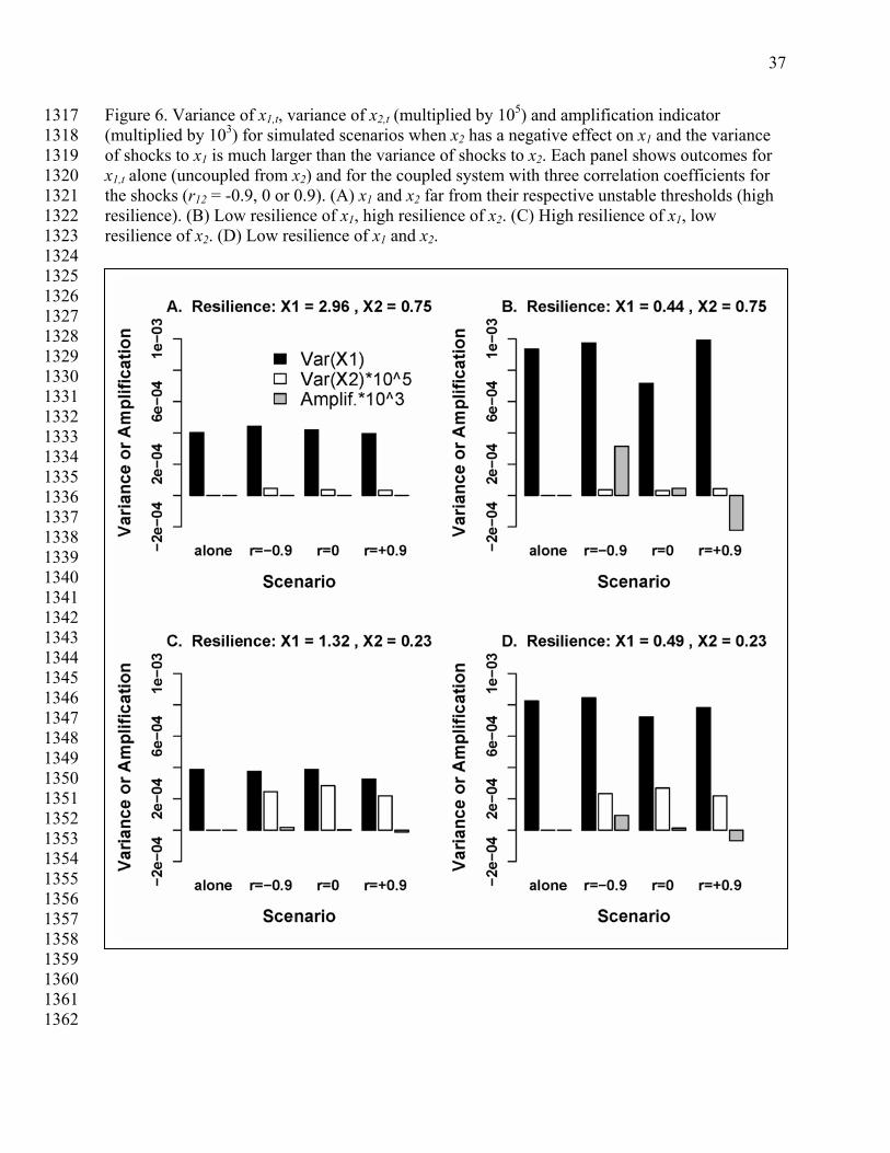
37

Figure 6. Variance of x1,t, variance of x2,t (multiplied by 105) and amplification indicator 1317 (multiplied by 103) for simulated scenarios when x2 has a negative effect on x1 and the variance 1318 of shocks to x1 is much larger than the variance of shocks to x2. Each panel shows outcomes for 1319 x1,t alone (uncoupled from x2) and for the coupled system with three correlation coefficients for 1320 the shocks (r12 = -0.9, 0 or 0.9). (A) x1 and x2 far from their respective unstable thresholds (high 1321 resilience). (B) Low resilience of x1, high resilience of x2. (C) High resilience of x1, low 1322 resilience of x2. (D) Low resilience of x1 and x2. 1323 1324 1325 1326 1327 1328 1329 1330 1331 1332 1333 1334 1335 1336 1337 1338 1339 1340 1341 1342 1343 1344 1345 1346 1347 1348 1349 1350 1351 1352 1353 1354 1355 1356 1357 1358 1359 1360 1361 1362

38

1363 Figure 7. Variance of x1,t, variance of x2,t (multiplied by 105) and amplification indicator 1364 (multiplied by 103) for simulated scenarios when x2 has a positive effect on x1 and the variance of 1365 shocks to x1 is much larger than the variance of shocks to x2. Each panel shows outcomes for x1,t 1366 alone (uncoupled from x2) and for the coupled system with three correlation coefficients for the 1367 shocks (r12 = -0.9, 0 or 0.9). (A) x1 and x2 far from their respective unstable thresholds (high 1368 resilience). (B) Low resilience of x1, high resilience of x2. (C) High resilience of x1, low 1369 resilience of x2. (D) Low resilience of x1 and x2. 1370 1371 1372 1373 1374 1375 1376 1377 1378 1379 1380 1381 1382 1383 1384 1385 1386 1387 1388 1389 1390 1391 1392 1393 1394 1395 1396 1397 1398 1399 1400 1401 1402 1403 1404 1405 1406 1407 1408