inteligencia de negocio - welcome to the sci2s...
TRANSCRIPT
1
INTELIGENCIA DE NEGOCIO 2017 - 2018
Tema 1. Introducción a la Inteligencia de Negocio
Tema 2. Minería de Datos. Ciencia de Datos
Tema 3. Modelos de Predicción: Clasificación, regresión y series temporales
Tema 4. Preparación de Datos
Tema 5. Modelos de Agrupamiento o Segmentación
Tema 6. Modelos de Asociación
Tema 7. Modelos Avanzados de Minería de Datos.
Tema 8. Big Data
2
Modelos avanzados de Minería de Datos
Objetivos:
• Analizar diferentes extensiones del problema de clasificación clásico de acuerdo a diferentes problemas reales que plantean un nuevo escenario en los problemas de clasificación.
• Introducir brevemente estas extensiones.
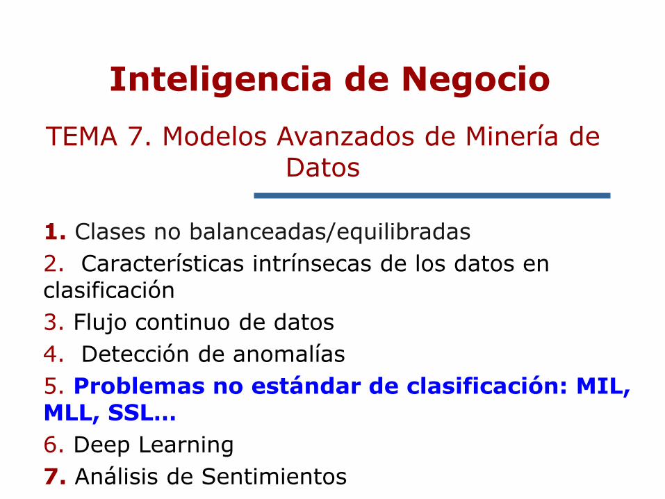
1. Clases no balanceadas/equilibradas
2. Características intrínsecas de los datos en clasificación
3. Flujo continuo de datos
4. Detección de anomalías
5. Problemas no estándar de clasificación: MIL, MLL, SSL…
6. Deep Learning
7. Análisis de Sentimientos
Inteligencia de Negocio
TEMA 7. Modelos Avanzados de Minería de Datos

4
Nuevos problemas de clasificación
•Técnicas avanzadas: Ensembles (Bagging, Boosting), Pruning, …
•Multiclases: OVA, OVO
• Múltiples etiquetas
• Múltiples instancias
• Ranking de clases
• Clasificación ordinal y monotónica, semisupervisada, multiview learning, …
• Discretización
• Selección de características
• Selección de instancias
•Reducción de la dimensionalidad
•Datos imperfectos: Valores perdidos, Ruido de clase y variable
•Clases no equilibradas
• Baja densidad de datos–
• small disjuncts
• Overlapping entre clases
• Dataset Shift -
• Particionamiento
• Medidas de Complejidad
•TÉCNICAS DE CLASIFICACIÓN: Árboles decisión: C4.5, Sistemas basados en reglas, Clasificación basada en instancias (k-NN, …), regresión logística, SVM, RNN, One-class, modelos probabilísticos,
Nuevos problemas
No-estandar

5
MIL: Multi-instance learning
ML: Multi-label classification
Monotonic Classification
Semisupervised Learning
Nuevos problemas de clasificación

From ML to MIL: Conventional Machine Learning Model Decision Problem

From ML to MIL: Conventional Machine Learning Model Decision Problem
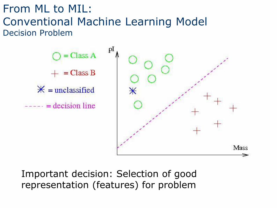
Important decision: Selection of good representation (features) for problem
From ML to MIL: Conventional Machine Learning Model Decision Problem
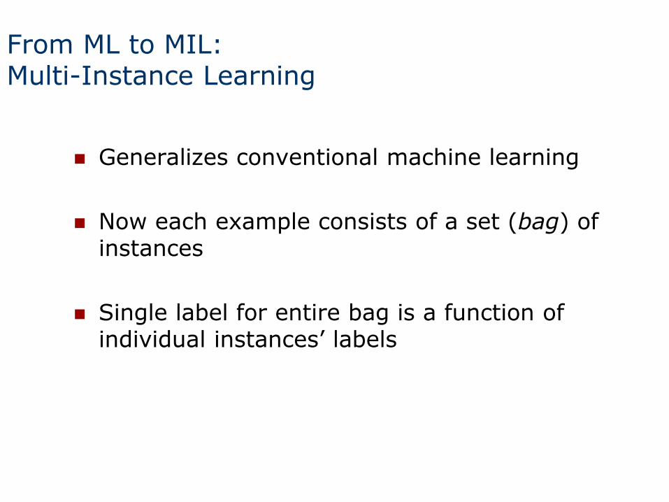
Generalizes conventional machine learning
Now each example consists of a set (bag) of instances
Single label for entire bag is a function of individual instances’ labels
From ML to MIL: Multi-Instance Learning

Originated from the research on drug activity prediction
[Dietterich et al. AIJ97]
Drugs are small molecules working by binding to the target area
For molecules qualified to make the drug, one of its shapes could tightly bind to the target area
A molecule may have many alternative shapes
The difficulty:
Biochemists know that whether a molecule is qualified or not, but do not know which shape responses for the qualification
Figure reprinted from [Dietterich et al., AIJ97] [Dietterich et al., 1997] T. G. Dietterich, R.
H. Lathrop, T. Lozano-Perez. Solving the Multiple-Instance Problem with Axis-Parallel Rectangles. Artificial Intelligence Journal, 89, 1997.
From ML to MIL: Multi-Instance Learning

Each shape can be represented by a feature vector, i.e., an instance
A bag is positive if it contains at least one positive instance; otherwise it is negative
The labels of the training bags are known
The labels of the instances in the training bags are unknown
Thus, a molecule is a bag of instances
…
[a1, a2, …, am]T
[b1, b2, …, bm]T
[u1, u2, …, um]T
…
one bag one molecule
Figure reprinted from [Zhi-Hua Zhou et al., icml09]
From ML to MIL: Multi-Instance Learning
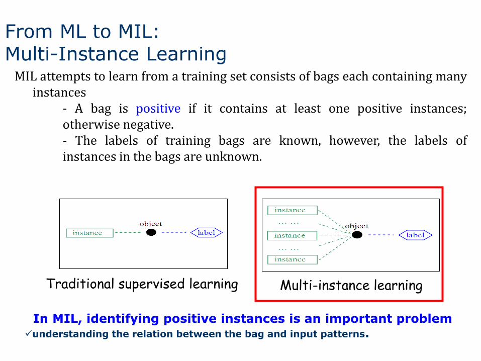
MIL attempts to learn from a training set consists of bags each containing many instances
- A bag is positive if it contains at least one positive instances; otherwise negative. - The labels of training bags are known, however, the labels of instances in the bags are unknown.
Multi-instance learning Traditional supervised learning
In MIL, identifying positive instances is an important problem understanding the relation between the bag and input patterns.
From ML to MIL: Multi-Instance Learning

Multiple-instances Single table
Examples as sets
Each instance is a person
Each set describes a family
Examples, e.g.
class(neg) :- person(aa,aa,aa,AA),
person(aa,aa,aa,aa).
or
{person(aa,aa,aa,AA), person(aa,aa,aa,aa) }
From ML to MIL: Multi-Instance Learning

Citation kNN
Support Vector Machine for multi-instance learning
Multiple-decision tree
… …
Learning approaches
See: http://link.springer.com/book/10.1007%2F978-3-319-47759-6
Multiple-Instance Learning

15
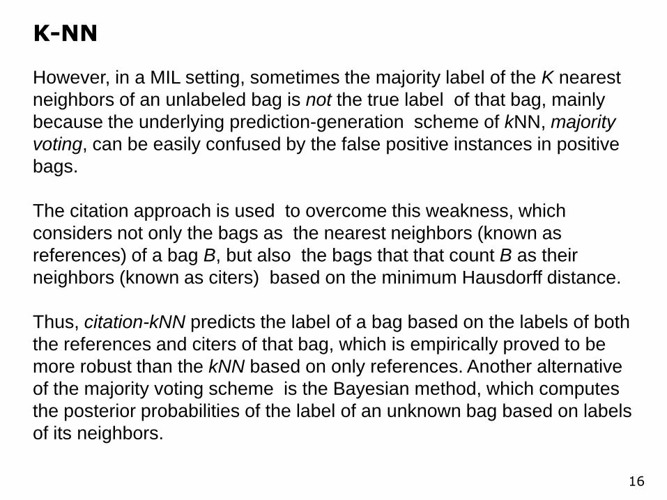
Citation K-NN
The popular k Nearest Neighbor (k-NN) approach can be adapted for
MIL problems if the distance between bags is defined.
In [Wang and Zucker, 2000], the minimum Hausdorff distance
was used as the bag-level distance metric, defined as the shortest
distance between any two instances from each bag.
where A and B denote two bags, and a_i and b_j are instances from each
bag.
Using this bag-level distance, we can predict the label of an
unlabeled bag using the k-NN algorithm.
16
K-NN
However, in a MIL setting, sometimes the majority label of the K nearest
neighbors of an unlabeled bag is not the true label of that bag, mainly
because the underlying prediction-generation scheme of kNN, majority
voting, can be easily confused by the false positive instances in positive
bags.
The citation approach is used to overcome this weakness, which
considers not only the bags as the nearest neighbors (known as
references) of a bag B, but also the bags that that count B as their
neighbors (known as citers) based on the minimum Hausdorff distance.
Thus, citation-kNN predicts the label of a bag based on the labels of both
the references and citers of that bag, which is empirically proved to be
more robust than the kNN based on only references. Another alternative
of the majority voting scheme is the Bayesian method, which computes
the posterior probabilities of the label of an unknown bag based on labels
of its neighbors.

Drug activity prediction
Content-based image retrieval and classification
… …
Applications
Multiple-Instance Learning

Iterated-discrim APR [Dietterich et al., 1997]
Diverse Density (DD) [Maron and Lozano-Perez, 1998]
EM-DD [Zhang and Goldman, 2001]
Two SVM variants for MIL [Andrews et al., 2002]
Citation-kNN for MIL [Wang and Zucker, 2000]
… …
Software
http://www.cs.cmu.edu/~juny/MILL/index.html
MILL: A Multiple Instance Learning Library Developed by:
Jun Yang School of Computer Science Carnegie Mellon University
Multiple-Instance Learning
19
MIL: Multi-instance learning
ML: Multi-label classification
Monotonic Classification
Semisupervised Learning
Nuevos problemas de clasificación

Motivation: Multi-label objects
Text classification is everywhere
Web search
News classification
Email classification
……
Many text data are multi-labeled
Business
Politics
Entertainment
Travel
World news
Local news
… …

Motivation: Multi-Label Objects
Lake
Trees
Mountains
Multi-label learning
e.g. natural scene image
Documents, Web pages, Molecules......

Traditional single-label classification is concerned with
learning from a set of examples that are associated with a
single label l from a set of disjoint labels L, |L| > 1.
In multi-label classification, the examples are associated
with a set of labels Y in L.
In the past, multi-label classification was mainly
motivated by the tasks of text categorization and medical
diagnosis. Nowadays, we notice that multi-label classification
methods are increasingly required by modern applications,
such as protein function classification, music categorization
and semantic scene classification.
22
Multi-label classification
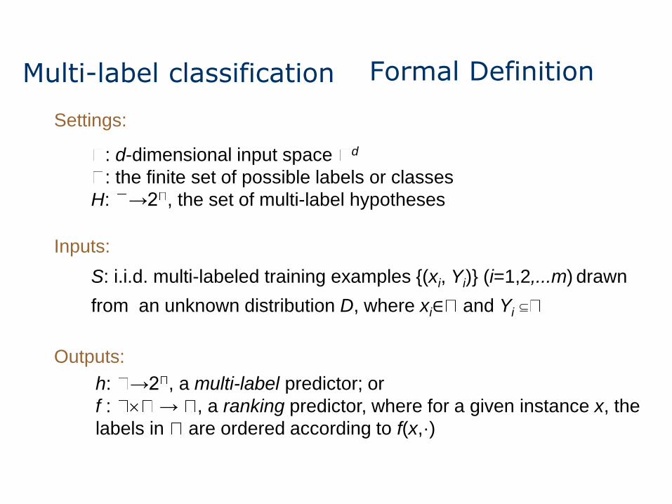
Formal Definition
Settings:
: d-dimensional input space d
: the finite set of possible labels or classes
H: →2 , the set of multi-label hypotheses
Inputs:
S: i.i.d. multi-labeled training examples {(xi, Yi)} (i=1,2,...m) drawn
from an unknown distribution D, where xi∈ and Yi
Outputs:
h: →2 , a multi-label predictor; or
f : → , a ranking predictor, where for a given instance x, the
labels in are ordered according to f(x,·)
Multi-label classification

Evaluation Metrics
Given:
S: a set of multi-label examples {(xi, Yi)} (i=1,2,...m), where
xi∈ and Yi
f : → , a ranking predictor (h is the corresponding
multi-label predictor)
Hamming Loss:
One-error:
Coverage
Ranking Loss:
Average Precision:
1
1hamloss ( ) ( )
m
S i i
i
f h x Ym k
0 1 1 0
1
1 1rankloss ( ) , | ( , ) ( , )
m
S i i i i
i i i
f l l Y Y f x l f x lm Y Y
' '
1
| ( , ) ( , )1 1avgprec ( )
| | {1,..., } | ( , ) ( , )i
mi i i
S
i l Yi i i
l Y f x l f x lf
m Y j k f x j f x l
1
1one -err ( ) | ( ) , where ( )=argmax ( , )
m
S i ili
f i H x Y H x f x lm
Y
1
1coverage ( ) max ( , ) 1
i
m
S f iy Y
i
f rank x ym Î
=
= -å
Definitions:
Multi-label classification

BoosTexter
Extensions of AdaBoost
Convert each multi-labeled example into many binary-labeled examples
Maximal Margin Labeling
Convert MLL problem to a multi-class learning problem
Embed labels into a similarity-induced vector space
Approximation method in learning and efficient classification algorithm in testing
Probabilistic generative models
Mixture Model + EM
PMM
Text Categorization
Learning approaches, applications, software

Extended Machine Learning Approaches
ADTBoost.MH
Derived from AdaBoost.MH [Freund & Mason, ICML99]
and ADT (Alternating Decision Tree) [Freund & Mason, ICML99]
Use ADT as a special weak hypothesis in AdaBoost.MH
Rank-SVM
Minimize ranking loss criterion while at the same have a large
margin
Multi-Label C4.5
Modify the definition of entropy
Learn a set of accurate rules, not necessarily a set of complete
classification rules
ML k-NN
Learning approaches, applications, software

Java library for Multi-label learning, called Mulan
Mulan is hosted at SourceForge, so you can grab latest releases
from there, as well as the latest development source code from
the project's public SVN repository.
There is a collection of several multilabel datasets, properly
formatted for use with Mulan.
… …
Software: Mulan: An Open Source Library for Multi-Label Learning
http://mlkd.csd.auth.gr/multilabel.html
Learning approaches, applications, software

28
MIL: Multi-instance learning
ML: Multi-label classification
Monotonic Classification
Semisupervised Learning
Nuevos problemas de clasificación
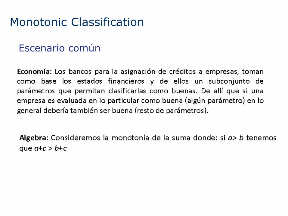
Monotonic Classification
Escenario común

Monotonic Classification

Monotonic Classification
Restricción monotónica

Monotonic Classification
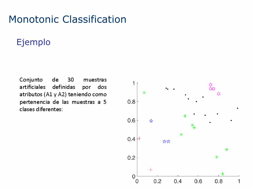
Monotonic Classification
Ejemplo

34
MIL: Multi-instance learning
ML: Multi-label classification
Monotonic Classification
Semisupervised Learning
Nuevos problemas de clasificación
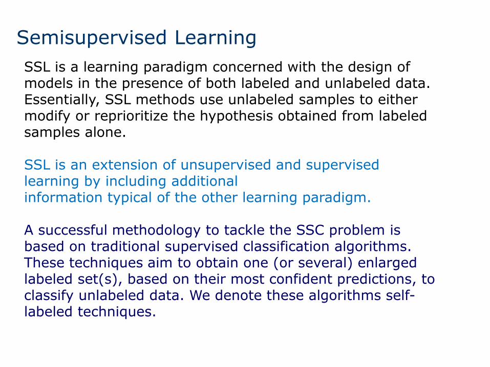
Semisupervised Learning
SSL is a learning paradigm concerned with the design of models in the presence of both labeled and unlabeled data. Essentially, SSL methods use unlabeled samples to either modify or reprioritize the hypothesis obtained from labeled samples alone. SSL is an extension of unsupervised and supervised learning by including additional information typical of the other learning paradigm. A successful methodology to tackle the SSC problem is based on traditional supervised classification algorithms. These techniques aim to obtain one (or several) enlarged labeled set(s), based on their most confident predictions, to classify unlabeled data. We denote these algorithms self-labeled techniques.

Semisupervised Learning
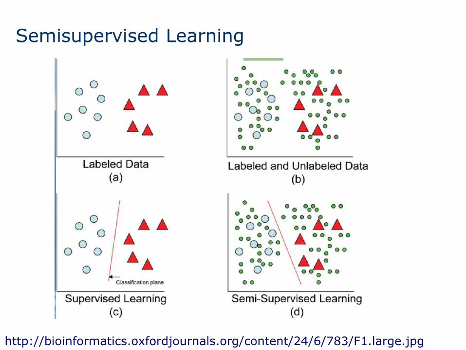
Semisupervised Learning
http://bioinformatics.oxfordjournals.org/content/24/6/783/F1.large.jpg

38
Others: Multi-view learning
Nuevos problemas de clasificación
Multi-view learning is concerned with the problem of machine learning from data represented by multiple distinct feature sets.
Example: http://www.mcrlab.net/wp-content/uploads/2015/08/framework.jpg
multi-view sentiment analysis.

39
Others: Multi-view learning
Nuevos problemas de clasificación
Multi-view learning is concerned with the problem of machine learning from data represented by multiple distinct feature sets.
Example: http://www.mcrlab.net/wp-content/uploads/2015/08/framework.jpg
multi-view sentiment analysis.

40
Others: Weak supervision and other non-standard classification problems: A taxonomy
Nuevos problemas de clasificación

1. Clases no balanceadas/equilibradas
2. Características intrínsecas de los datos en clasificación
3. Flujo continuo de datos
4. Detección de anomalías
5. Problemas no estándar de clasificación: MIL, MLL, SSL…
6. Deep Learning
7. Análisis de Sentimientos
Inteligencia de Negocio
TEMA 7. Modelos Avanzados de Minería de Datos
Comentario final: Estas son algunas de las extensiones al problema clásico de clasificación.
Muchas aparecen como consecuencia de nuevos problemas reales que requieren de un nuevo planteamiento de clasificación.
1. Clases no balanceadas/equilibradas
2. Características intrínsecas de los datos en clasificación
3. Flujo continuo de datos
4. Detección de anomalías
5. Problemas no estándar de clasificación: MIL, MLL, SSL…
6. Deep Learning
7. Análisis de Sentimientos
Inteligencia de Negocio
TEMA 7. Modelos Avanzados de Minería de Datos

43
Outline What are anomalies?
Anomaly Detection: Taxonomy
Nearest Neighbor Based Techniques
One-Class to tackle the Fault Detection
Concluding Remarks
Anomaly Detection
44
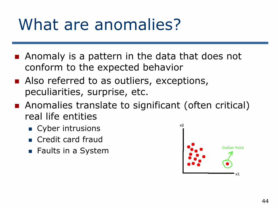
What are anomalies?
Anomaly is a pattern in the data that does not conform to the expected behavior
Also referred to as outliers, exceptions, peculiarities, surprise, etc.
Anomalies translate to significant (often critical) real life entities
Cyber intrusions
Credit card fraud
Faults in a System
45
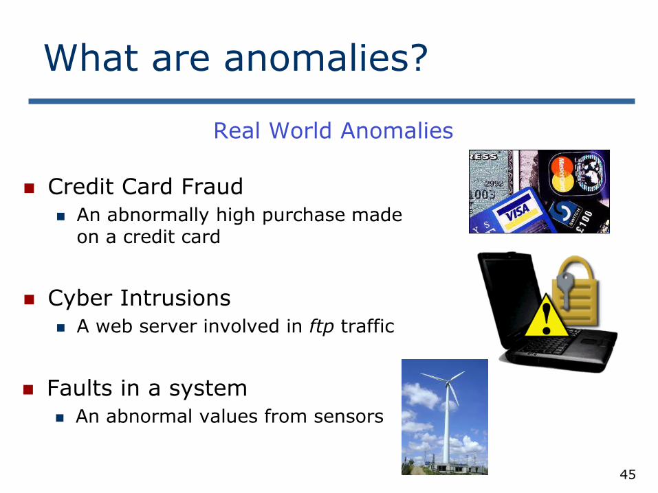
What are anomalies?
Real World Anomalies
Credit Card Fraud
An abnormally high purchase made on a credit card
Cyber Intrusions
A web server involved in ftp traffic
Faults in a system
An abnormal values from sensors

Simple Example
N1 and N2 are regions of normal behavior
Points o1 and o2 are anomalies
Points in region O3 are anomalies
X
Y
N1
N2
o1
o2
O3
What are anomalies?

Related problems
Rare Class Mining (high imbalanced classes)
Chance discovery
Novelty Detection
Exception Mining
Noise Removal
Black Swan*
* N. Talleb, The Black Swan: The Impact of the Highly Probable?, 2007
What are anomalies?

Key Challenges
Defining a representative normal region is challenging
The boundary between normal and outlying behavior is often not precise
The exact notion of an outlier is different for different application domains
Availability of labeled data for training/validation
Malicious adversaries
Data might contain noise
Normal behavior keeps evolving
What are anomalies?

Aspects of Anomaly Detection Problem
Nature of input data
Availability of supervision
Type of anomaly: point, contextual, structural
Output of anomaly detection
Evaluation of anomaly detection techniques
What are anomalies?

Type of Anomaly
Point Anomalies
Contextual Anomalies
Collective Anomalies
What are anomalies?
V. CHANDOLA, A. BANERJEE, and VI. KUMAR. Anomaly Detection: A Survey ACM Computing Surveys, Vol. 41, No. 3, Article 15, Publication date: July 2009.
http://doi.acm.org/10.1145/ 1541880.1541882

Point Anomalies
An individual data instance is anomalous w.r.t. the data
X
Y
N1
N2
o1
o2
O3
What are anomalies?
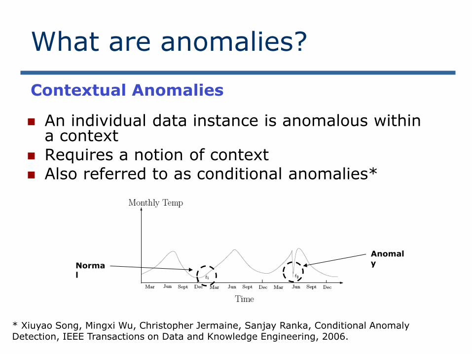
Contextual Anomalies
An individual data instance is anomalous within a context
Requires a notion of context Also referred to as conditional anomalies*
* Xiuyao Song, Mingxi Wu, Christopher Jermaine, Sanjay Ranka, Conditional Anomaly Detection, IEEE Transactions on Data and Knowledge Engineering, 2006.
Normal
Anomaly
What are anomalies?
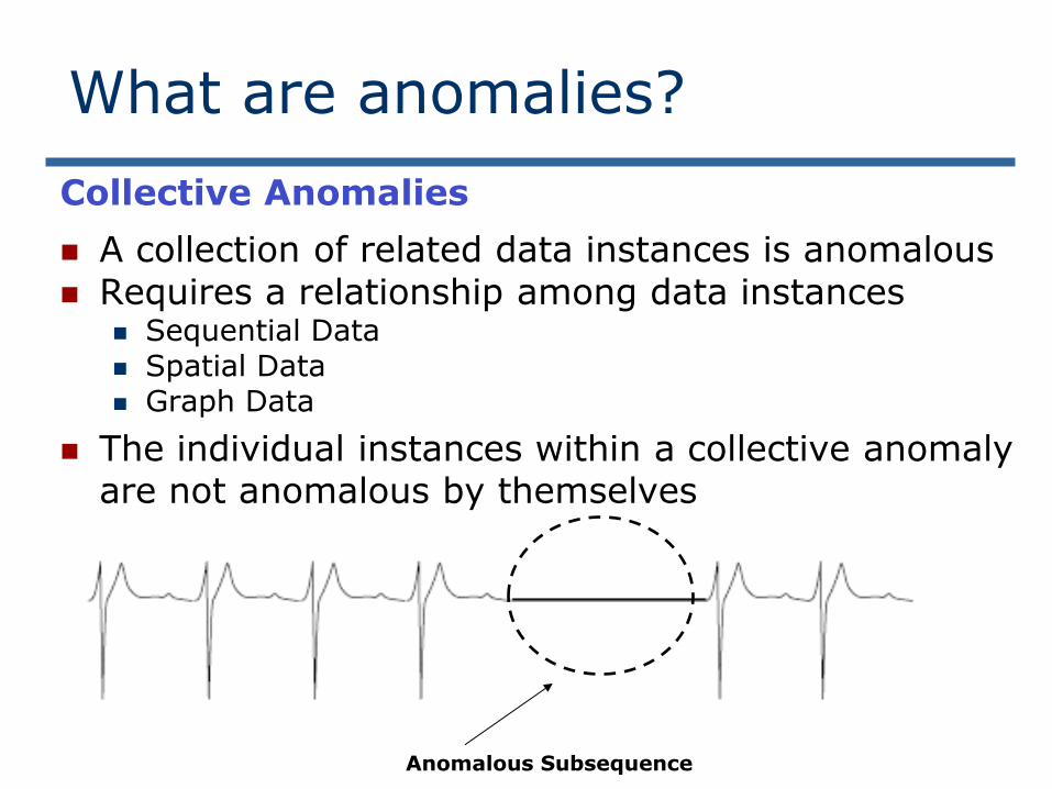
Collective Anomalies
A collection of related data instances is anomalous Requires a relationship among data instances
Sequential Data Spatial Data Graph Data
The individual instances within a collective anomaly are not anomalous by themselves
Anomalous Subsequence
What are anomalies?

Applications of Anomaly Detection
Network intrusion detection
Insurance / Credit card fraud detection
Healthcare Informatics / Medical diagnostics
Industrial Damage Detection
Image Processing / Video surveillance
Novel Topic Detection in Text Mining
…
What are anomalies?
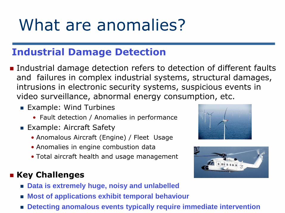
Industrial Damage Detection
Industrial damage detection refers to detection of different faults and failures in complex industrial systems, structural damages, intrusions in electronic security systems, suspicious events in video surveillance, abnormal energy consumption, etc.
Example: Wind Turbines
• Fault detection / Anomalies in performance
Example: Aircraft Safety
• Anomalous Aircraft (Engine) / Fleet Usage
• Anomalies in engine combustion data
• Total aircraft health and usage management
Key Challenges
Data is extremely huge, noisy and unlabelled
Most of applications exhibit temporal behaviour
Detecting anomalous events typically require immediate intervention
What are anomalies?
56
Outline What are anomalies?
Anomaly Detection: Taxonomy
Nearest Neighbor Based Techniques
One-Class to tackle the Fault Detection
Concluding Remarks
Anomaly Detection

Anomaly Detection
Contextual Anomaly Detection
Collective Anomaly Detection
Online Anomaly Detection Distributed Anomaly Detection
Point Anomaly Detection
Classification Based
Rule Based
Neural Networks Based
SVM Based
Nearest Neighbor Based
Density Based
Distance Based
Statistical
Parametric
Non-parametric
Clustering Based Others
Information Theory Based
Spectral Decomposition Based
Visualization Based
* Anomaly Detection – A Survey, Varun Chandola, Arindam Banerjee, and Vipin Kumar, ACM Computing Surveys, Vol. 41, No. 3, Article 15, Publication date: July 2009.
Anomaly Detection: Taxonomy

Classification Based Techniques
Main idea: build a classification model for normal (and anomalous (rare)) events based on labeled training data, and use it to classify each new unseen event
Classification models must be able to handle skewed (imbalanced) class distributions
Categories:
Supervised classification techniques
• Require knowledge of both normal and anomaly class
• Build classifier to distinguish between normal and known anomalies
Semi-supervised classification techniques
• Require knowledge of normal class only!
• Use modified classification model to learn the normal behavior and then detect any deviations from normal behavior as anomalous
Anomaly Detection: Taxonomy

Classification Based Techniques Advantages:
Supervised classification techniques
• Models that can be easily understood
• High accuracy in detecting many kinds of known anomalies
Semi-supervised classification techniques
• Models that can be easily understood
• Normal behavior can be accurately learned
Drawbacks:
Supervised classification techniques
• Require both labels from both normal and anomaly class
• Cannot detect unknown and emerging anomalies
Semi-supervised classification techniques
• Require labels from normal class
• Possible high false alarm rate - previously unseen (yet legitimate) data records may be recognized as anomalies
Anomaly Detection: Taxonomy

Supervised Classification Techniques
Rule based techniques
Model based techniques
Neural network based approaches
Support Vector machines (SVM) based approaches
Bayesian networks based approaches
Imbalanced classification
Manipulating data records (oversampling / undersampling / generating artificial examples)
Cost-sensitive classification techniques
Ensemble based algorithms (SMOTEBoost, RareBoost
Anomaly Detection: Taxonomy

Creating new rule based algorithms
Adapting existing rule based techniques
Robust C4.5 algorithm [John95]
Adapting multi-class classification methods to single-class classification problem
Association rules
Rules with support higher than pre specified threshold may characterize normal behavior
Anomalous data record occurs in fewer frequent itemsets compared to normal data record
Frequent episodes for describing temporal normal behavior [Lee00,Qin04]
Case specific feature/rule weighting
Increasing the rule strength for all rules describing the rare class or features strength for highlighting the minority class.
Rule Based Techniques
Anomaly Detection: Taxonomy
63
Outline What are anomalies?
Anomaly Detection: Taxonomy
Nearest Neighbor Based Techniques
One-Class to tackle the Fault Detection
Concluding Remarks
Anomaly Detection

64
All instances correspond to points in the n-D space. The nearest neighbor are defined in terms of Euclidean
distance. The target function could be discrete- or real- valued. For discrete-valued, the k-NN returns the most common
value among the k training examples nearest to xq. Voronoi diagram: the decision surface induced by 1-NN for
a typical set of training examples.
. _
+ _ xq
+
_ _ +
_
_
+
.
. .
. .
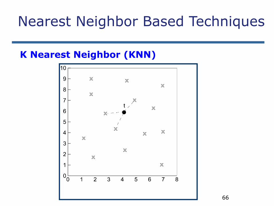
K Nearest Neighbor (KNN)
Nearest Neighbor Based Techniques

65
K Nearest Neighbor (KNN)
Training set includes classes.
Examine K items near item to be classified.
New item placed in class with the most number of close items.
O(q) for each tuple to be classified. (Here q is the size of the training set.)
Nearest Neighbor Based Techniques
66
K Nearest Neighbor (KNN)
Nearest Neighbor Based Techniques
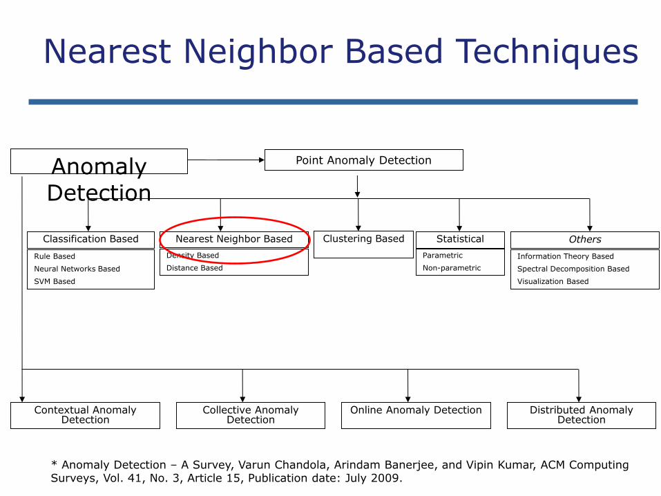
Anomaly Detection
Contextual Anomaly Detection
Collective Anomaly Detection
Online Anomaly Detection Distributed Anomaly Detection
Point Anomaly Detection
Classification Based
Rule Based
Neural Networks Based
SVM Based
Nearest Neighbor Based
Density Based
Distance Based
Statistical
Parametric
Non-parametric
Clustering Based Others
Information Theory Based
Spectral Decomposition Based
Visualization Based
* Anomaly Detection – A Survey, Varun Chandola, Arindam Banerjee, and Vipin Kumar, ACM Computing Surveys, Vol. 41, No. 3, Article 15, Publication date: July 2009.
Nearest Neighbor Based Techniques
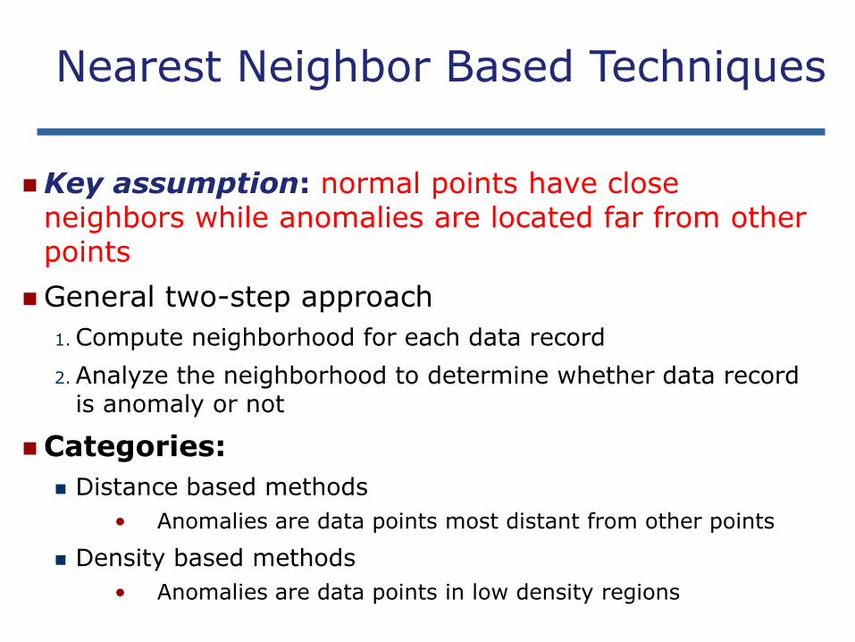
Key assumption: normal points have close neighbors while anomalies are located far from other points
General two-step approach
1. Compute neighborhood for each data record
2. Analyze the neighborhood to determine whether data record is anomaly or not
Categories:
Distance based methods
• Anomalies are data points most distant from other points
Density based methods
• Anomalies are data points in low density regions
Nearest Neighbor Based Techniques

Advantage
Can be used in unsupervised or semi-supervised setting (do not make any assumptions about data distribution)
Drawbacks
If normal points do not have sufficient number of neighbors the techniques may fail
Computationally expensive
In high dimensional spaces, data is sparse and the concept of similarity may not be meaningful anymore. Due to the sparseness, distances between any two data records may become quite similar => Each data record may be considered as potential outlier!
Nearest Neighbor Based Techniques

Distance based approaches
A point O in a dataset is an DB(p, d) outlier if at least fraction p of the points in the data set lies greater than distance d from the point O*
Density based approaches
Compute local densities of particular regions and declare instances in low density regions as potential anomalies
Approaches
• Local Outlier Factor (LOF)
• Connectivity Outlier Factor (COF
• Multi-Granularity Deviation Factor (MDEF)
Nearest Neighbor Based Techniques
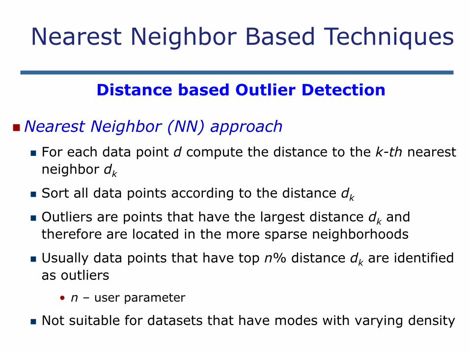
Distance based Outlier Detection
Nearest Neighbor (NN) approach
For each data point d compute the distance to the k-th nearest
neighbor dk
Sort all data points according to the distance dk
Outliers are points that have the largest distance dk and
therefore are located in the more sparse neighborhoods
Usually data points that have top n% distance dk are identified
as outliers
• n – user parameter
Not suitable for datasets that have modes with varying density
Nearest Neighbor Based Techniques

Density Based Approaches: Local Outlier Factor (LOF)
For each data point q compute the distance to the k-th nearest
neighbor (k-distance)
Compute reachability distance (reach-dist) for each data example q with respect to data example p as:
reach-dist(q, p) = max{k-distance(p), d(q,p)}
Compute local reachability density (lrd) of data example q as inverse of the average reachabaility distance based on the MinPts nearest neighbors of data example q
lrd(q) =
Compute LOF(q) as ratio of average local reachability density of q’s k-nearest neighbors and local reachability density of the data record q
LOF(q) =
p
MinPts pqdistreach
MinPts
),(_
p qlrd
plrd
MinPts )(
)(1
Nearest Neighbor Based Techniques

Advantages of Density based Techniques
Local Outlier Factor (LOF) approach
Example:
p2 p1
In the NN approach, p2 is not considered as outlier, while the LOF approach find both p1 and p2 as outliers
NN approach may consider p3 as outlier, but LOF approach does not
p3
Distance from p3 to nearest neighbor
Distance from p2 to nearest neighbor
Nearest Neighbor Based Techniques
74
Outline What are anomalies?
Anomaly Detection: Taxonomy
Nearest Neighbor Based Techniques
One-Class to tackle the Fault Detection
Concluding Remarks
Anomaly Detection

Several classes vs One-class classification
One-Class to tackle the Fault Detection

Classification Based Techniques Advantages:
Supervised classification techniques
• Models that can be easily understood
• High accuracy in detecting many kinds of known anomalies
Semi-supervised classification techniques (One-class)
• Models that can be easily understood
• Normal behavior can be accurately learned
Drawbacks:
Supervised classification techniques
• Require both labels from both normal and anomaly class
• Cannot detect unknown and emerging anomalies
Semi-supervised classification techniques (One-class)
• Require labels from normal class
• Possible high false alarm rate - previously unseen (yet legitimate) data records may be recognized as anomalies
One-Class to tackle the Fault Detection

One-Class to tackle the Fault Detection
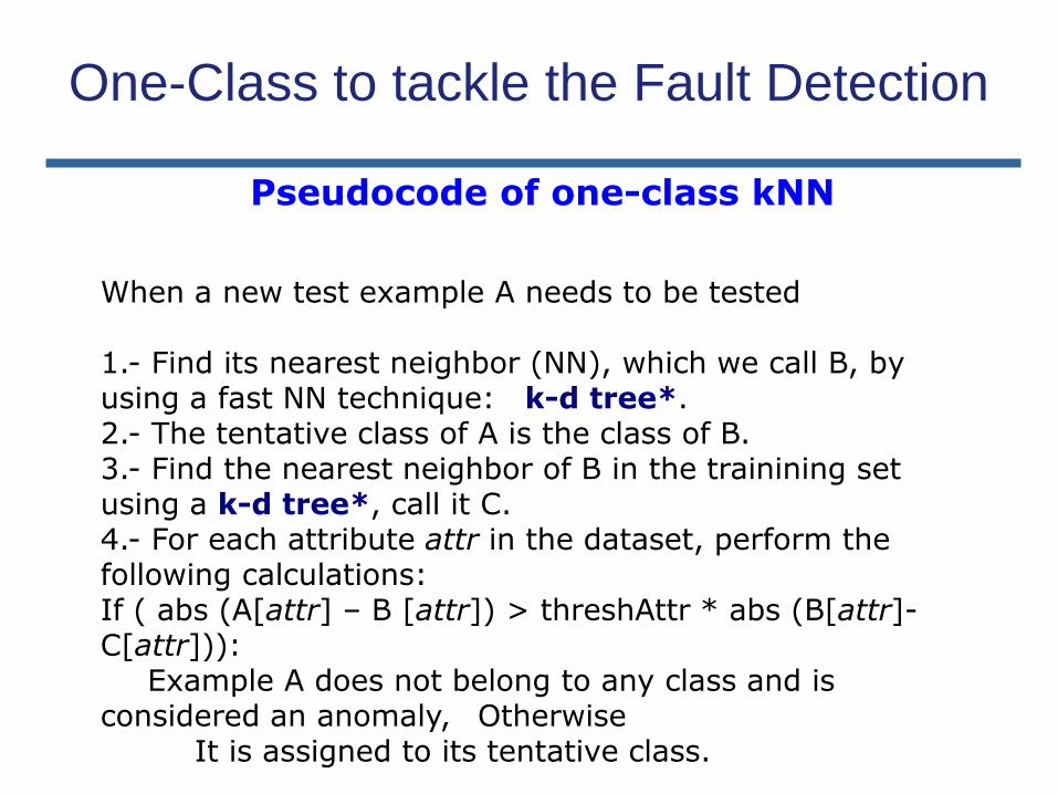
One-class 1-NN is an semi-supervised algorithm that learns a decision function for novelty detection: classifying new data as similar or different to the training set.
Pseudocode of one-class kNN
When a new test example A needs to be tested 1.- Find its nearest neighbor (NN), which we call B, by using a fast NN technique: k-d tree*. 2.- The tentative class of A is the class of B. 3.- Find the nearest neighbor of B in the trainining set using a k-d tree*, call it C. 4.- For each attribute attr in the dataset, perform the following calculations: If ( abs (A[attr] – B [attr]) > threshAttr * abs (B[attr]-C[attr])): Example A does not belong to any class and is considered an anomaly, Otherwise It is assigned to its tentative class.
One-Class to tackle the Fault Detection
A1
Constructing a k-d tree
A0
A1 A1
A0<=0.45 A0>0.45 A0<=0.45
A2 A2 A2 e05
e07 e01 e02 e04
e06
e03
A1<=0.2 A1>0.2
A1>0.54 A1<=0.54
<=0.12 >0.12 >0.35
<=0.35
<=0.45
>0.45
One-Class to tackle the Fault Detection

Visually: Training examples
Normal examples
Iddling examples
One-Class to tackle the Fault Detection
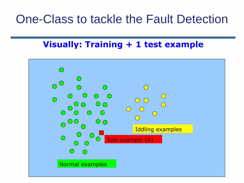
Visually: Training + 1 test example
Normal examples
Iddling examples
Test example (A)
One-Class to tackle the Fault Detection
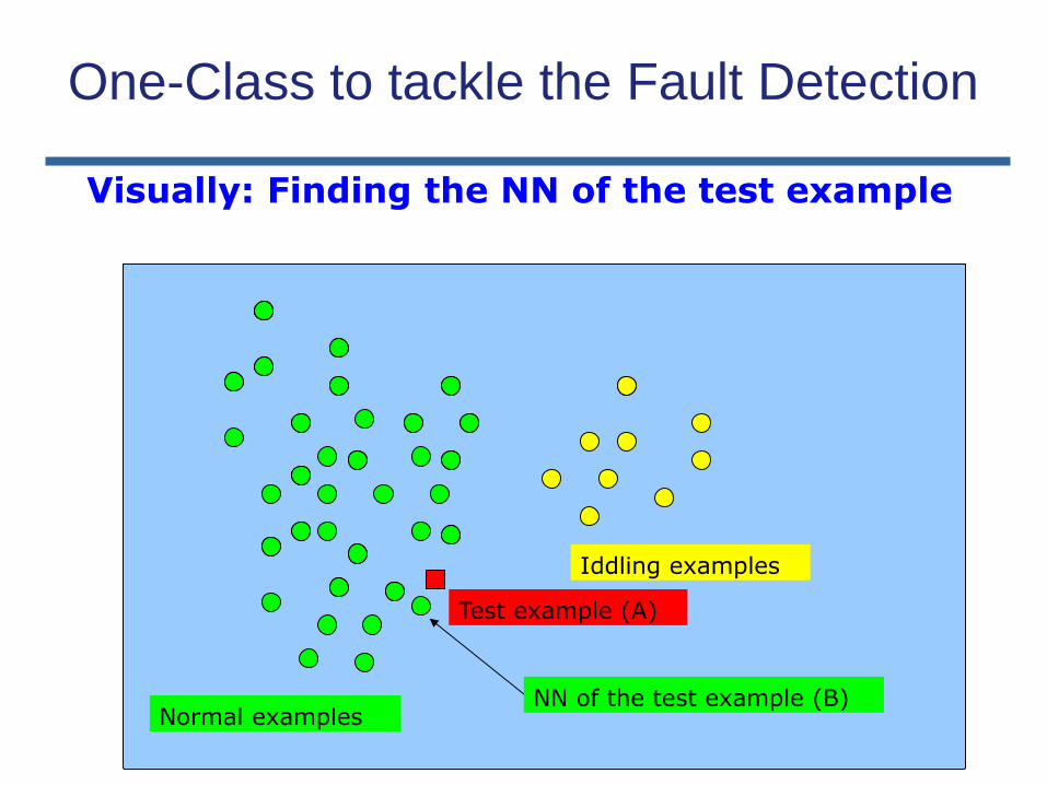
Visually: Finding the NN of the test example
Normal examples
Iddling examples
Test example (A)
NN of the test example (B)
One-Class to tackle the Fault Detection

Visually: Finding the NN of B (finding C)
Normal examples
Iddling examples
Test example (A)
NN of the test example (B)
NN of the NN (C)
One-Class to tackle the Fault Detection
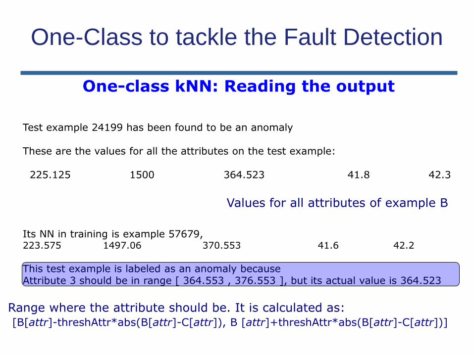
Test example 24199 has been found to be an anomaly These are the values for all the attributes on the test example: 225.125 1500 364.523 41.8 42.3 Its NN in training is example 57679, 223.575 1497.06 370.553 41.6 42.2
This test example is labeled as an anomaly because Attribute 3 should be in range [ 364.553 , 376.553 ], but its actual value is 364.523
Values for all attributes of example B
One-class kNN: Reading the output
One-Class to tackle the Fault Detection
Range where the attribute should be. It is calculated as: [B[attr]-threshAttr*abs(B[attr]-C[attr]), B [attr]+threshAttr*abs(B[attr]-C[attr])]

Brief tutorial on k-d trees
Basic idea: binary tree where each node splits the data in two subgroups with roughly half the size (divide and conquer) How? Take an attribute, split the data points by the median value: The examples with value under or equal to the median are placed on the subtree to one side, those with values over the median go to the subtree on the other side. The size of the tree is O(n), the average time to find a match (a Nearest Neighbor, the process is explained in the next slide) is O(log(n)). In this context, n refers to the number of examples in the training set. The time to find a match is on average O(log(n)) only when the k-d tree works well. For a k-d tree to work well, the number of examples must be much larger than the number of attributes (n should be >= 2nAttr), and said examples should be approximately randomly distributed. Both of these conditions hold in the HMS-GAMESA data, so the k-d tree is a very good solution for this problem.
One-Class to tackle the Fault Detection

Constructing a k-d tree (I) Example data (each row corresponds to an example, each column is an attribute):
Root node: take attribute A0. Median = 0.45. e01, e02, e04 and e07 go to the left subtree, e03, e05 and e06 to the right one.
Second level: attribute A1. On the left subtree the median is 0.20, e01 and e07 go left and e02, e04 go right. On the right subtree, the median is 0.54. e03 and e06 go left, e05 goes right.
Repeat the process until all examples are on leaves.
Example ID A0 A1 A2 A3
e01 0.10 0.06 0.20 0.30
e02 0.30 0.33 0.35 0.51
e03 0.50 0.65 0.54 0.45
e04 0.45 0.14 0.56 0.89
e05 0.52 0.17 0.67 0.64
e06 0.53 0.40 0.45 0.11
e07 0.29 0.54 0.12 0.54
One-Class to tackle the Fault Detection

A1
A0
A1 A1
A0<=0.45 A0>0.45 A0<=0.45
A2 A2 A2 e05
e07 e01 e02 e04
e06
e03
A1<=0.2 A1>0.2
A1>0.54 A1<=0.54
<=0.12 >0.12 >0.35
<=0.35
<=0.45
>0.45
Constructing a k-d tree (II)
One-Class to tackle the Fault Detection
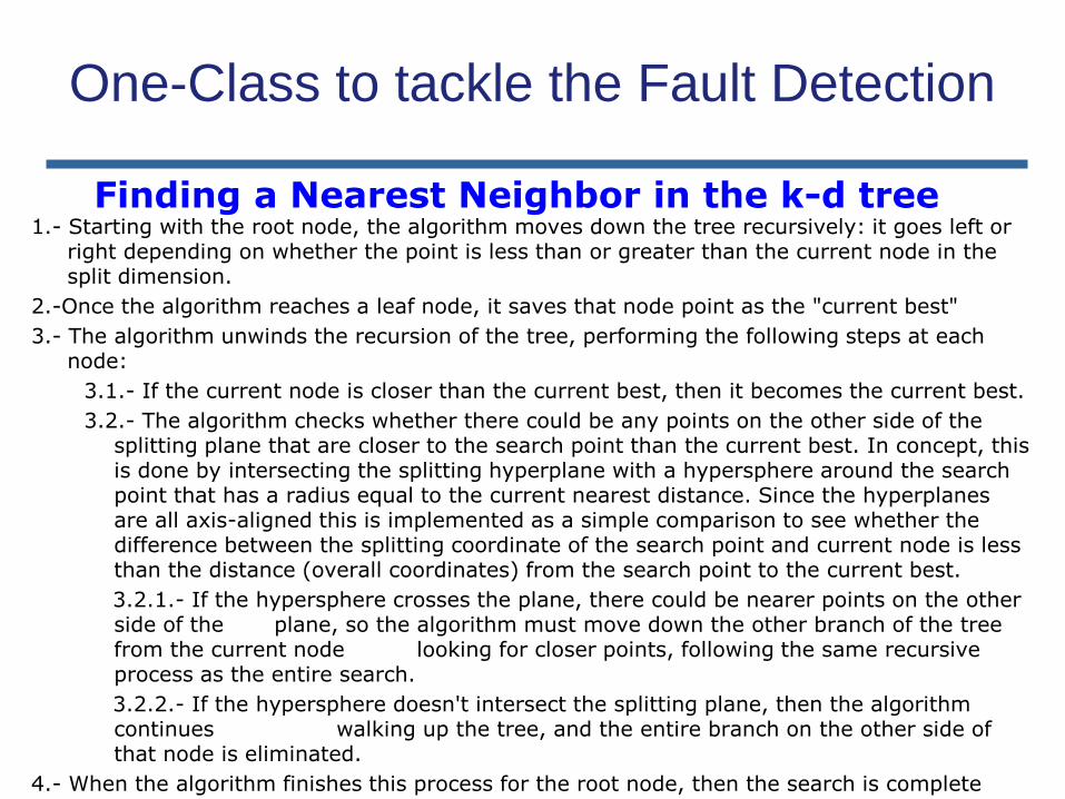
Finding a Nearest Neighbor in the k-d tree 1.- Starting with the root node, the algorithm moves down the tree recursively: it goes left or
right depending on whether the point is less than or greater than the current node in the split dimension.
2.-Once the algorithm reaches a leaf node, it saves that node point as the "current best"
3.- The algorithm unwinds the recursion of the tree, performing the following steps at each node:
3.1.- If the current node is closer than the current best, then it becomes the current best.
3.2.- The algorithm checks whether there could be any points on the other side of the splitting plane that are closer to the search point than the current best. In concept, this is done by intersecting the splitting hyperplane with a hypersphere around the search point that has a radius equal to the current nearest distance. Since the hyperplanes are all axis-aligned this is implemented as a simple comparison to see whether the difference between the splitting coordinate of the search point and current node is less than the distance (overall coordinates) from the search point to the current best.
3.2.1.- If the hypersphere crosses the plane, there could be nearer points on the other side of the plane, so the algorithm must move down the other branch of the tree from the current node looking for closer points, following the same recursive process as the entire search.
3.2.2.- If the hypersphere doesn't intersect the splitting plane, then the algorithm continues walking up the tree, and the entire branch on the other side of that node is eliminated.
4.- When the algorithm finishes this process for the root node, then the search is complete
One-Class to tackle the Fault Detection

89
Outline What are anomalies?
Anomaly Detection: Taxonomy
Nearest Neighbor Based Techniques
One-Class to tackle the Fault Detection
Concluding Remarks
Anomaly Detection

Conclusions
Anomaly detection can detect critical information in data
Highly applicable in various application domains
Nature of anomaly detection problem is dependent on the
application domain
Need different approaches to solve a particular problem
formulation
The nearest neighbor based techniques are very appropriate for
different problems, but they need to be tuned to this problem.

Conclusions
Related topic: Novelty detection

INTELIGENCIA DE NEGOCIO 2017 - 2018
Tema 1. Introducción a la Inteligencia de Negocio
Tema 2. Minería de Datos. Ciencia de Datos
Tema 3. Modelos de Predicción: Clasificación, regresión y series temporales
Tema 4. Preparación de Datos
Tema 5. Modelos de Agrupamiento o Segmentación
Tema 6. Modelos de Asociación
Tema 7. Modelos Avanzados de Minería de Datos
Tema 8. Big Data