integrating logistics and production

Integrating logistics and production

Management Engineering Department

Master’s thesis


Student: Víctor Rabasa Martínez

Professor: Peter Jacobsen

Date: 30 of June 2017


Abstract

The purpose of this research project is to help a supply chain manager to decision making easier

in order to deliver final product on time to final customer. Coordination between all members

of a supply chain are essential to achieve this objective and reduce bullwhip effect. The members

considered on this thesis are going to be a manufacture, its supplier and supplier of that supplier

(sub-supplier). A common purchase forecast is done thanks to Collaborative Planning

Forecasting and Replenishment (CPFR) using an order point policy. A dashboard is elaborated

with Key Performance Indicators (KPI) and graphics that shows the status of the supply chain.

Then a simulation of a real case test how robust is the supply chain using normal random

variables and evaluate how good and reliable are each of the members of the supply chain. At

the end of the project there is a little experiment where a supply chain is checked with two

different scenarios in which stability of demand are different. The results of that projects show

an easy to use dashboard which evaluate a supply chain and its members and gives numerical

and graphic information to the manager.


Index

1.Introduction ............................................................................................................................... 1

2. Problem situation ...................................................................................................................... 4

2.1. Problem statement ............................................................................................................ 4

3. Literature review ....................................................................................................................... 5

3.1. Integrated supply chain and purchase management......................................................... 5

3.2. Dashboard .......................................................................................................................... 6

3.3. CPFR (Collaborative Planning Forecasting Replenishment) ............................................... 8

3.4. Supplier evaluation ............................................................................................................ 9

3.5. Stock control .................................................................................................................... 11

4. Analysis .................................................................................................................................... 12

4.1. Necessary information for controlling a supply chain ..................................................... 12

4.1.1. Manufacture or supplier ........................................................................................... 12

4.1.4. Customer ................................................................................................................... 15

4.1.3. Transport ................................................................................................................... 16

4.2. Methodology .................................................................................................................... 18

4.2.1. Limitations: ................................................................................................................ 18

4.2.2. Considerations:.......................................................................................................... 18

4.2.3. Nomenclature............................................................................................................ 19

4.2.4. Initial data.................................................................................................................. 20

4.2.5. Order point purchase forecasting policy ................................................................... 21

4.2.6. Simulation method .................................................................................................... 25

4.3. Evaluating supply chain using KPI’s .................................................................................. 30

5. Use of results ........................................................................................................................... 34

6. Discussion ................................................................................................................................ 39

7. Experiment .............................................................................................................................. 40

8. Conclusions.............................................................................................................................. 48

9. Bibliography ............................................................................................................................ 49

10. Acknowledgments .................................................................... ¡Error! Marcador no definido.


1

1.Introduction

A supply chain is an entire network of entities, directly or indirectly interlinked and

interdependent in serving the same consumer or customer. It comprises of vendors that supply

raw material, producers who convert the material into products, warehouses that store,

distribution centres that deliver to the retailers, and retailers who bring the product to the

ultimate user. Supply chains underlie value-chains because, without them, no producer can give

customers what they want, when and where they want, at the price they want. Producers

compete only through their supply chains, and no degree of improvement at the producer's end

can make up for the deficiencies in a supply chain which reduce the producer's ability to

compete.

A supply chain management is basically about planning and controlling the activities of a

company in order to secure that the right product is delivered in the right quantities to the right

costumer at the right time to the right price. It is necessary for a company to have each step of

that long chain as integrated and coordinated as possible.

A Just in time purchasing policy is generally the best choice to buy raw materials because it

usually minimizes the total costs of total purchasing compared with Economic Order Quantity

policy. Even though a Just in Time policy is the most efficient purchasing policy a priori not always

can assure that will not break stock and it clashes with the idea of deliver product on time.

On the other hand, Economic order quantity policy (EOQ) depends on the policy of each member

of the supply chain. Anyway, all purchase policy can fail if the forecasting of the manufacture

doesn’t take in account free production availability, production capacity or stock level of its

supplier. So, in order to make an easier and common purchase policy, an order point purchase

policy is going to be used in the whole supply chain.

Discoordination of each element of a supply chain that has optimized its stock level and its

purchasing policy independently from other members is known as bullwhip effect. In other

words, although your purchase forecasting is optimized, it can crash with the availability of the

supplier in one specific moment on time line.

To mitigate this discoordination there is one possible solution that many companies have

implemented and have shown to be very effective, the Collaborative Planning Forecasting and

Replenishment (CPRF). This system implies the collaboration of each component of the supply

chain on sharing its internal, confidential and sensitive information like demand forecasting,

production capacity, production status, level stock…etc.

This solution has a difficulty to solve it because usually all suppliers tend to save all its internal

information to avoid industrial espionage and to avoid lose competitiveness against its

competitor. Nevertheless, each component of supply chain will have to construct trust

relationships among them if they will want to survive in a long-term period, otherwise whole

supply chain won’t be able to satisfy the final costumer and won’t survive against other

competitors.

The idea is to create a common purchase forecasting in a month for manufacture, supplier and

sub-supplier in a just in time policy, that guarantees that every member has an optimized


2

purchase policy that reduces the stock cost and, at the same time, guarantee that all production

can be delivered at the right time.

It is entirely important for a supply chain to have a good coordination among each part that

belongs to it. Regarding to suppliers it is especially important this coordination in order to reduce

the bullwhip effect. For that reason, sharing information among these agents will be an essential

task for the whole supply chain.

One of the biggest problems that a manufacture company can suffer in his business is not to be

able to satisfy its client because it doesn’t have product available in its stock. In this project, the

idea is to face this problem attacking one of its root, the purchasing forecasting in a dashboard.

The main goal of this project is to be able to assure customer receives his order in the agreed

quantity and date.

A problem to control a supply chain is how to manage data extracted from production system

and convert it to a useful and clear information for someone who must make decisions

consequently. The more data received from a production system doesn’t directly mean that a

manager’s will be able to take the proper decisions. The elaboration and presentation of that

information will allow to a manager get the idea of what’s happening, where is the source of the

problem if exists and what responses are the most effective in a specific circumstance. A solution

for this presentation of the information it’s a dashboard where not only appear data from a

supply chain but also it appears post processed and presented in diagrams, tables, schemes and

KPI’s (Key Performance Indicator).

The aim of this project is to create a dash board for a supply chain manager who wants to have

under control all its parts. The objective is to gather all information in real time in one control

panel that allows to a manager knows whether his production system will be able to deliver a

purchase order on time and detect a problem before it occurs.

The reason of using a dashboard is to help supply chain managers to have all information in a

way that makes it easier for them to make a better decision regarding the current state of the

supply chain and the convenience of making a purchase order to a supplier in a specific time. If

a manager receives information of his supply chain in a simply way it will be easier for him

understanding the situation and taking a faster decision.

This dashboard would allow to manager to take structured and non-structured decisions. As an

example of structured decision would be about the feasibility to accept or refuse a purchase

order or knowing if one delivery will be on time or in case that this were not possible how much

time of delay it would have. The information system gives the opportunity for a user to manage

if it is necessary to change the order of the purchase order from their list of purchases made for

its customers.

Summary of information in a control panel would be also a source of information for the process

improvement department and open a door to detect which part of a supply chain are a bottle

neck of the production system and where is necessary to put more effort on improve it. An

integration of all this information in one information system would be a tool that may help on a

better coordination of a supply chain and could detect its collapse before it occurs.

The Supply Chain Operations Reference model (SCOR) is the world’s leading supply chain

framework, linking business processes, performance metrics, practices and people skills into a

unified structure. That model is a tool to represent, analyse and configure the Supply Chains.


3

The Model provides a unique framework that brings together Business Processes, Management

Indicators, Best Practices and Technologies in a unified structure to support communication

between Supply Chain Partners and improve the efficiency of Supply Chain Management (GSC)

and the improvement of related activities of the Supply Chain (SC). The Model has been able to

provide a basis for SC improvement in global projects as well as specific localized projects,

including a homogeneous set of related processes.

The SCOR is a Reference Model that standardizes the terminology and processes of an SC for

modelling, using KPIs (Key Performance Indicators), to compare and analyse different

alternatives and strategies of SC entities and of the whole SC.

The SCOR model allows to describe the business activities necessary to satisfy customer

demand, and is organized around five Main Processes of Management: Planning, Source,

Manufacturing, Deliver, and Return.


4

2. Problem situation

The problem that is set out in this project is to create a dashboard among a sub-supplier, a

supplier and a manufacturer. It will be constructed with information supplied by both parts so

that It will mean that collaboration is essential in order to get an information resource for both.

The coordination of every entity will be determined by the decisions made on the basis of that

panel, so in case of incoordination it will be easier for both managers to detect and discuss what

decisions has been done wrongly and what kind of corrective measures have to be taken to

avoid it.

The dashboard will be created on costumer direction, that it means that the main goal is final

client satisfaction through a deliver on time. Both companies will have the same information to

take decisions to satisfy the final client.

The KPIs in the dashboard will be based on SCOR (Supply Chain Operations Reference Model).

This KPIs must help supplier and manufacturer to organise themselves around the five main

processes of management: planning, source, manufacturing, deliver and return.

When an order is placed at a producer and the producer has to give a specific delivery time he

needs to be sure that his suppliers can deliver at the right time. If the promised delivery time is

exceeded the producer will often pay a fee. A dashboard will support the producer in making

his decision.

2.1. Problem statement

"How can dashboard be designed for a supply chain?" In order to design a dashboard, different indicators need to be identified together with the

interrelationship between them. Also, the significant indicators (KPI) needs to be identified as

they will be presented at the dashboard. Supplement questions could therefore be,

• How can the different indicators be identified? • Can the different indicators be grouped? • What is the relation between the indicators? • What is the significant indicators? • How can they be presented on a dashboard? • How can the dashboard be maintained?


5

3. Literature review

This theory section contains review and description of various literature of purchase

management, supply chain management, dashboards, supplier collaboration or CPFR

(Collaborative Planning Forecasting and Replenishment), supplier evaluation and stock control.

Related to the concepts above, I will proceed to explain each of them for a previous better

understanding. Supply chain will be described as a set of members that need to be coordinated

in order to achieve a main goal. The main goal is to deliver the final product to the final costumer

at the right time. After that, an overview about how a dashboard with processed information

can help a manager to take the proper decision at the proper time. Afterwards, the CPFR will

be presented as the essential tool to develop the idea for coordinating and improving the whole

supply chain, and to minimise the total product costs. At the end of section I will show how

stock control can help for making the supply chain more efficient and less expensive at the same

time.

3.1. Integrated supply chain and purchase management

When a product order takes place at the producer, and the producer must give a specific delivery

time, he needs to make sure that his suppliers can deliver it at the right time. If the pointed

delivery time is exceeded the producer will normally pay a fee.

One of the problems that a manufacture must afford for being successful is the Purchase

Management. Therefore, if raw materials don’t arrive on time, the supply chain and the client’s

satisfaction may be in risk of breaking up, and it could turn into sales loses for the company.

(Jahnukainen & Lahti, 1999) says that “The efficiency on purchase area determine the price of a

product directly” and demonstrates the proved background that “a supply chain may perform

unsatisfactorily although the individual units in the chain are performing well”. Therefore, he

gives three viable solutions. To control the suppliers as if they were our own manufacture,

having special arrangements for critical components, and the integration and cooperation of

members of a supply chain.

Keeping all this inputs in mind, the objective of this project is to convert these three purchase

areas: manufacture, supplier and sub-supplier, into a unique centralised purchase forecasting

program on a simple dashboard. The integration and cooperation on forecasting purchase

orders will be the main point of this project, so I will treat the supplier’s forecasting as ours.


6

The economic lot size policy based on JIT, developed by (Yang, Wee, & Yang, 2007), state that

for an integrated buyer-vendor system, the inventory cost and the reply time of an order must

be reduced.

(Rau & OuYang, 2008) developed a model of purchasing based on a “just at time” acquisition of

raw materials. This model proposes a single buyer - single vendor relation at a restricted amount

of time system. It also shows how the delivery time might be affected by the model.

The model succeeds by minimizing the shared total costs incurred by the vendor and the buyer,

and prove the optimal way to perform to achieve a linear increasing or decreasing demand

solution.

It also shows that the performance of the integrated consideration is better than the

performance of any independent decision made by either, the buyer or the vendor.

JIT purchase policy is usually the best policy to minimize purchasing costs and to optimize the

stock level. However, (Wu, 2007) has demonstrated that JIT system is not always better

regarding cost effectiveness than EOQ (Economic Order Quantity). Despite, EOQ could be better

than JIT in some specific cases.

3.2. Dashboard

The reason for constructing a dashboard for a purchase forecasting is to have all the information

of the supply chain summarised just in one panel. It also provides managers with a view of your

current status, so you can anticipate the worst scenarios and perform to succeed.

The use of appropriate indicators can help the managers to be more responsive to the

dashboard signals. The OEE monitoring in manufacturing plants is discussed by (Anand, 2010)

stating that “Faster response can reduce machine downtime; improve machine performance and

overall plant efficiency”. For that reason, not always the data presented by itself can help to a

manager, so KPIs could help to take faster decisions.

(El Farouk Imane, Foaud, & Abdennebi, 2017) present a methodology called OPRI (Objectives,

Parameters, Risk, Indicators) to build a medicine supply chain dashboard for public hospitals.

This methodology is based on process modelling using SCOR (Supply Chain Operations

Reference), ARIS and risk analysis.

(Franceschini & Turina, 2012) propose a methodology that show how to merge the existing

Performance Measurement System to define a unique shared reference system and provide a

general performance dashboard in order to monitor WaSCs (Water and Sewage Companies).

It is developed in order to assist regulators with a small set of critical indicators (performance

dashboard) for the evaluation and monitorization of the service.


7

(Goh et al., 2013) propose a real-time risk monitoring based on real-time data collection and

analysis. The Risk Vis is based on multi-hierarchy modular design. It helps to monitor and collect

real-time risky information that contains both internal and external manufacture data.

This information may help the managers to make better and safer decisions in order to avoid

the break of the supply chain if any unexpected event happens.

Regarding that, it would be kept in mind that suppliers are usually supplied by another sub-

supplier. That means that if there happen any unexpected event or issue in any of the steps of

this chain, all the chain will be affected, and consequently it would affect the customer’s delivery

time directly with all their consequences.

The article of (Karr, 2012) has shown that those who are engaged in collaboration with a supplier

will be rewarded with superior profits and stronger relationships, which are critical to the market

success and for having a growing platform. It says that dashboards are essential not just for the

manufacture, but for the suppliers. The dashboard should be created in collaboration between

the supplier and the buyer for the best effectiveness. The importance of having the right and

common metrics for both determines the relationship between the buyer and the supplier.

“Dashboards work best if there is senior management support for a customer-supplier

relationship process that uses relationship and strategic performance dashboards”. That proves

that forecasting of purchasing must be done by a buyer-supplier collaboration.

A very accurate example of a good dashboard based on the SCOR model is shown by (Pretorius,

Ruthven, & Von Leipzig, 2013) applied to an egg producer placed in South Africa which captures

the trend of the different performance attributes of the supply chain.

The model serves to facilitate the transition from local and functional management control to a

wide supply chain management participation and approach before engaging it in a full-scale

SCOR implementation. The way this article presents the results using both KPl’s and graphics,

will be used in this project to show the data and results in our dashboard at the most effortless

way.

The United Nations World Food Program’s Supply Chain Management Dashboard, as known as

SCM-D, is described by (Sithole, Silva, & Kavelj, 2016). One of the objectives and values of that

organization is to ensure a zero-hunger world society. Its work is founded by three pillars: to

increase operational efficiency and effectiveness by enhancing the supply chain visibility; to

finance the organisation through donation founds; and to provide overall services to those in

need.


8

(Strandhagen & Dreyer, 2006) present the concept of an ICT based supply chain dashboard. It

may benefit to get access to a real-time monitoring facilities, to speed up recognition and to an

integrated decision making. All those inputs give a true value supply chain perspective.

3.3. CPFR (Collaborative Planning Forecasting Replenishment)

As we already know, bullwhip effect is the result of a discoordination of each component in a

supply chain which has optimized its stock level and its purchasing policy independently from

the other members. Discoordination may become bigger when the supply chain becomes longer

and other entities are added into the chain: that increases the problem’s complexity.

Many methods and projects have appeared in order to mitigate this effect between a supplier

and a manufacture. One of these is CPFR, where manufacture and suppliers work together to

get a better synergy. CPFR is a management process in which supply chain participants

collaborate in the preparation of sales forecasts and replenishment plans for greater visibility.

This process improves the synchronization of the actions related to the sales forecast and the

planning of the supplies for all the participants. It allows to reduce the level of stocks and

improve the rate service towards the final customer.

The objective of (A. Kubde, 2012) is to shed light on the collaborative relationships between

buyers and sellers and its impact on supply chain performance. It explores the domain of CPRF

for optimizing supply chain performance. In addition, it says that in the future all companies will

must adopt any kind of partnerships initiative with suppliers. The bullwhip effect can be reduced

with information sharing and demand forecasting between the supplier and the buyer.

As (Ji & Liu, 2010) state, CPFR emphasize on the importance of the cooperation and partnership

theory regarding the supply chain strategies, but theoretically the application process is not as

satisfactory as it is forecasted.

Regarding this problem, demand is not having that importance yet, so there aren’t still very clear

solutions for sales and orders forecast steps. In a short-term future, CPFR model is going to be

used by a lot of companies in order to cover their own needs.

(Kreng & Chen, 2017) apply a three-echelon supply chain between manufacturer, delivery centre

and retailer focused on the order quantity, shipment sizes and number of shipments.

The results of the study state that compared with a typical delivery policy, all supply chain stages

collaboration and the agreement of applying the optimal shipping size will totally improve the

cost reduction.

(J. T. Lin, Chang, Chen, & Xin, 2003) study the KPI flow and data flow from CPFR system, applied

to the relationship between two Taiwan companies. Once you implement CPFR system, CMC


9

and the buyer may collaborate planning, forecasting and refilling according to the forecasted

demand.

Besides, in the CPFR system, seller and buyer may solve exceptions in collaboration.

Consequently, buyer and seller may collaborate in planning, forecasting and refilling according

to the forecasted demand.

The article also analyses the CPFR related information system for designing a better KPI

information flow. In that case, there are four KPI used: order forecast accuracy, finished goods

production lead-time, on time delivery and order fill rate. A successful KPI flow design may show

the improving performance to facilitate efficiency in supply chain.

Applying CPFR system into a company is not as easy as it seems to be. It requires a business

processes change, as well as an inward change focusing into a broad multi-enterprise point of

view.

(Kubde & Bansod, 2010) suggest to the managers to investigate about the reasons for why, what

and how to manage in order to select the most appropriate decision for CPFR system. In

addition, in the study they ask you to call into question the theory and research practise in order

to find which are all the different CPFR activities. Finally, it concludes stating that in a short-term

future all organizations would adopt CPFR system.

3.4. Supplier evaluation

To manage, control and evaluate a whole supply chain starting with the sub supplier, continuing

with the supplier and finishing with the manufacturer is an idea that it’s applied in this project,

and have had few precedents in other literatures.

Supplier evaluation based on KPI is a common practise in many supply chains. That helps to

evaluate suppliers and its efficiency. Although this evaluation is based in historical data, it isn’t

always the best resource to evaluate a supplier in a specific period of time.

Knowing that a manufacture has a variety of different suppliers for each component it’s also

important to evaluate them in order to know which one is the most appropriate for a specific

command.

In this thesis project, the most relevant KPI item will be the delivery time, because the main

objective of the project is to make a forecast purchases’ dashboard without failing on delivery

time. Of course, it will take also into account some other KPIs as reliability, cost, etc.

When a purchased order is placed or forecasted sometimes the regular supplier responsible of

bringing the raw material to the buyer is not working as usual. There are two possible reasons.


10

Because the supplier may have a too large demand, or because supplier might have some

internal problems that doesn’t allow it. On the other hand, that might happen because of some

internal problems and is not the most appropriate moment to send a purchase order in spite of

is the one that normally works better.

(Bai & Sarkis, 2014) use DEA (Data Envelopment Analysis) as a comparative analysis to identify

sustainable supply chain KPI that could be used for a sustainable performance evaluation for

suppliers.

“Sustainability performance evaluation can be eased for managers by using KPIs, and then use

these KPIs to develop an easy and comparable performance measure”. It reinforces the idea of

comparative analysis between suppliers, so it means that before to forecast or to launch a

purchase order is a good idea to check which supplier is more suitable at a certain moment.

(Li, Lim, Chen, & Tan, 2016) examines existing approaches for supplier selection focused on its

advantages and limitations. The paper proposes an approach for supplier selection based on

selection criteria and Agent-Based Simulation (ABS) to address some of the limitations. The

proposed approach can be used to produce feasible supplier selection decisions which need to

consider multiple criteria and uncertainties. To do that could be difficult to be handled by the

traditional mathematic approaches. Those experiments show that the proposed approach can

be used for supplier selection through quantitative evaluation of the supplier profiles.

The selection and evaluation method for suppliers that (Pal & Kumar, 2008) uses for expensive

procurements provides a logical framework for supplier management based on Security,

Quality, Deliver and Cost. It transforms this items to a “Vendor Performance Dashboard” for

decision making.

The idea of (Pradhan & Routroy, 2014) was to identify the critical success factors and its

corresponding KPIs using the AHP. That can evaluate the performance of supplier development

that allows to get an approach for quantifying, monitoring, analysing and evaluating the success

of the SD programme.

“Supplier evaluation and selection must be systematically considered from the decision makers”

say (Xia & Lim, 2008), whose supplier selection method allows to reflect the supply chain

strategies of suppliers. Unlike other methods just can include quantitative factors, this method

allows qualitative factors as well.

(Ying, Lijun, & Wei, 2009) proposes some keys for establishing KPI to reflect supply chain

operations, and say that “By providing a simplified assessment of real-time supply chain

performance, dashboards change the speed and method in which executives enhance supply

chain execution”.


11

3.5. Stock control

Stock level is a crucial factor that help to a manufacture be successful for a specific delivery time,

the more stock levels a manufacture the less probability will have to fail if an unexpected rise of

demand appears. However, an increase of stock level usually involves of an increase level of cost

and decreased competitiveness in the company.

(Kang & Kim, 2010) presented a model for a supplier to control the inventory of its customer

through a vendor management inventory (VMI) that integers inventory replenishment and

deliver planning in an optimized way.

The purpose of (Y. C. E. Lin, 2006) is to explore the experience and results of companies that

manage logistics services to their chain convenience stores and their suppliers. It concludes

saying that the most crucial factor is an effective supply chain: “An efficient supply chain system

using e-Logistics is built on effective communication between stake holders”.

As (Raghavan, 2002) says, the aim of a supply chain is to produce and sell the desired products

in the proper delivery time, and studies some random network modelling techniques for

analysing supply chain networks. This study allows to compute lead times and to rely on every

facility of the chain.

(Zimmer, 2002) evaluates two situations of a supplier and a producer in a “just in time” environment

where the capacity of supplier is uncertain. In the first situation, they both don’t share information,

however on the second one they do. In that second case, it’s created a coordination system for a

centralised and non-centralised planner. It shows that in both cases the two costs can be equally low. It

also leaves one research field opened to include another step in the supply chain for the future. That is

what it’s being partially done in that thesis.


12

4. Analysis

4.1. Necessary information for controlling a supply chain

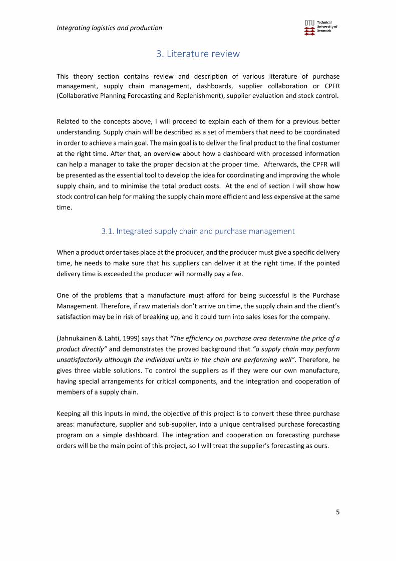
The objective of gathering information needs a reflection of what kind of information it is

necessary to don’t fail in the agreed delivery date, starting from suppliers and their suppliers,

the several types of transport used with raw materials and the final deliver:

Figure 1. Supply chain dashboard

4.1.1. Manufacture or supplier

An interchange of information with suppliers is crucial to create a good coordination of all the

system production and to decrease or eliminate the bullwhip effect. Moreover, the whole

supplier network has directly or indirectly impact on the provisioning of our production system,

this includes not only our direct suppliers but also suppliers of suppliers.

Hereinafter it is shown the essential information that members of supply chain should share:

Production of normal capacity (units / day)

It is essential for knowing how much workload it can be requested in a period. It is an information

that is important for selecting the main providers of a supply chain. If production of normal

capacity is too low the chain will be in risk of collapsing and suffer delay.


13

Maximum capacity of production (units / day)

In peak working periods is necessary to know how far the production system that one manage

can support. It is important not only for accept or refuse an order from a customer but also for

controlling costs.

Status of capacity in real time (units /day)

Must be kept in mind that the provider may not be working for just one customer, probably will

have more than one and its capacity will be fluctuating constantly whenever they receive

purchase orders from its customer portfolio. So, considering the status of capacity of suppliers

is necessary to know when and how much it is possible to request raw materials at some time.

Reliability Factory (probability that stops the production system) (%)

Uncertainty of the events that surround us is a probability that must be considered. There are

many factors that could interrupt our manufacturing system, i.e. break of a machine, electric

cut, fire…etc. The problem lies in its measurement and its certainty, so a good way to know it

would be based on the historical database. Instructions from the machine manufacturer that

has provided machines of the system production can help to calculate this percentage.

Purchase order initiated (units)

The work in progress in a factory at some point can determine the speed that a new purchase

order can be done. Work in progress can be an obstacle for the flow of a supply chain.

Purchase order without being initiated (units)

In most cases the providers will have a list of purchase orders from many costumers, this can

make a delay on the delivery. The amount of purchase orders that one has in its own system is

something that one can manage and order depending on hurry of each order.

Stock of raw materials of each component at real time (units)

Availability of raw materials will mark the efficacy of suppliers; this data can suppose the

impossibility or the feasibility to make a purchase order and have its quick response. The fact

that a production system can produce something reactively will be related with the amount of

stock that one has in its factory at some point.

Stock of finished product in warehouse and security stock level (units)

Level of stock of finished production is a positive indicator for controlling a supply chain, the

more finished production has in its possession, the more guarantees a supply chain will have for

receiving ware at time. However, it affects to the storage cost.

Capacity to store finished product (units)

Capacity of warehouse can be a bottle neck on a supply chain flow and can determine total cost

and capability for having a security stock reserved for a rising demand. The capacity of a

warehouse determines how much stock someone can have in his factory. It is also important to

manage and planning transport to the final costumer, so the less capacity of a warehouse can

involve make trips more often.


14

Capacity to store raw material (units)

As well as finished production warehouse, raw materials warehouse can be bottle neck if there

are not space enough. The warehouse capacity of raw materials will establish the amount of

production that a production system can assume. It also will be a fundamental data in order to

manage purchases and transports from purchasing area.

Demand forecasting based on historical information demand period (units/period)

Demand forecasting is essential when someone is planning purchase orders. Demand

determines the production of a factory, and consequently affects into its purchase management

and into purchase management of its customer. Share demand planning bring an opportunity

to manage purchases and decide if it is better to advance or delay them.

Percentage of defective raw materials (%)

Not all the raw materials received from suppliers satisfies the quality required from a purchaser

and must be a latent problem if it is not considered. As the reliability factory, percentage of

defective raw materials and defective units produced is difficult to measure and must be

measured by historical database.

Percentage of defective units produced (%)

Inevitably not all the production made by factory meets quality requirements, and not all

production can be served to clients with guarantees, therefore it is included this percentage on

the dashboard developing.

Number of suppliers that supplier has (units)

Complexity of supplier’s network makes more difficult the control of supply chain and is

important to have it under consideration.

Distance from supplier to factory (kilometre)

Proximity of suppliers determines the purchase planning and the costs related to that. It is also

important for knowing the quantity requested in every purchase order.

Number of units of products demanded by client (units)

It is the amount of product that a costumer has requested and the departure data that it has

planned on this project.

Agreed delivery date (time)

It is obvious that if someone is trying to prepare a delivery on time first of all needs to know how

much time is available to do it.

MRP product that we manufacture (units)

The complexity of different pieces that needs to be made will establish the complexity in number

of suppliers that a supply chain needs.


15

4.1.4. Customer

The last part of a supply chain is the costumer and the one that in this project needs be satisfied

on arriving.

Distance between our factory and the customer (km)

The further the final costumer is the more time it will takes for deliver.

Agreed delivery date (t)

It is the data who set deadlines and the departure data for an operative management of a

company.


16

Table 1. Information used for this project

4.1.3. Transport

Another valuable information for a supply chain that should be considered would be about

transport. However, transport is not going to be included in the model developed in that project.

Depending on the complexity of the MRP of the product and the kind of product that is being

manufactured the time of transport may have a relevant role in a whole supply chain. The

distance and the diverse ways of transport are also factors that affects to a supply chain directly.

Necessary information for a PFCR Supplier Factory Customer

Production of normal capacity (units / day) � � �

Maximum capacity of production (units / day) � � �

Status of capacity in real time (units /day) � � �

Reliability Factory (probability that stops the

production system) (%)� � �

Purchase order initiated (units) � � �

Purchase order without being initiated (units) � � �

Stock of raw material of each component at real

time (units)� � �

Stock of finished product in the warehouse and

security stock level (units)� � �

Capacity to store finished product (units) � � �

Capacity to store raw material (units) � � �

Demand forecasting based on historical

information demand period (units/period)� � �

Percentage of defective raw materials (%) � � �

Percentage of defective units produced (%) � � �

Number of suppliers that our supplier has (units) � � �

Distance from supplier to factory (kilometre) � � �

Agreed delivery date (t) � � �

Number of units of products demanded by client

(units)� � �

MRP product that we manufacture (units) � � �

Information used for this project


17

Above it is presented the most relevant data that should be considered:

Average time from ordering the transport to the beginning of the transport (t)

It is the time that it takes for example to arrive from the moment you give the order until it

arrives. Normally transport is outsourced so this is an important to keep in mind.

Maximum time from ordering the transport to the beginning of the transport (t)

The maximum time from ordering a carriage until it arrives can be very damaging in terms of

timeliness.

Average time it takes the carrier to bring the raw material warehouse of a vendor to our factory

(t)

This include the time of response of a supplier takes to bring the raw material.

Likelihood of suffering a delay transport (accident, traffic, weather conditions ... etc) (%)

The uncertainty of the transport conditions or even the total loss of goods.

Average time delay that the transport can suffer (time)

The transport can suffer delay because of wheatear, mechanical problems, etc.

Number of transport used in transport (train, boat, plane, truck, pipeline, etc ...) (t)

The more ways transport it is being used both for supplies and for delivery the more complexity

will be the whole transport.

Speed of the transport media (Km/h)

This data will determine how fast the goods will arrive to its destination.


18

4.2. Methodology

4.2.1. Limitations:

The method to ensure that suppliers are not going to fail on its delivery time that this project is

going to follow is start thinking that all demand of our suppliers that does not come from our

manufacture has preference regarding our demand. It means that if supplier must choose

between satisfy our demand or satisfy another customer demand, the supplier will always

choose to satisfy the other customer. For example, if a supplier has a capacity to produce of

seventy units per day and has a demand of fifty units of another customer and fifty units of our

manufacture, then the supplier will deliver fifty units to the other customer and twenty units to

our manufacture. Of course, this methodology does not follow a real situation, but in this project

the goal is to ensure delivering the production at the right time, so the methodology includes

the worst possible scenario.

Figure 2. Calculation steps of the tool

4.2.2. Considerations:

·All product elaborated on the method needs one unit of raw material to produce one unit of

finished product.

·The shared predicted demand of supplier and sub-supplier are considered constant during the

whole month.

·It’s assumed that production capacity of each member of the supply chain is constant during

the whole month.

1st: Manufature forecast:

Based on manufacturedemand, the purchasepredicted is calculated.

2nd: Supplier forecast:

Based on supplier andmanufacture needs, thepurchase predicted iscalculated.

3rd: Sub-supplier forecast:

Based on sub-supplier andsupplier needs, the purchasepredicted is calculated.

4th:Sub-supplier simulation:

It simulates a real situationthrough random variablesbased on sub-supplierforecast.

5th:Supplier simulation:

It simulates a real situationthrough random variablesbased on supplier forecastand sub-supplier simulation.

6th: Manufacturer simulation:

It simulates a real situationthrough random variables based on manufacture forecast and suppliersimulation.


19

·The transport time from each member is considered one day as a fixed variable.

·A provider only sends its ware if all lot of product �� is completed.

· There is no limit on warehousing of finished goods or raw materials in any of the three members

of the supply chain.

4.2.3. Nomenclature

� = {1, … ,30} All days of the month

� Specific day of the month

= {1,2,3} Manufacture, supplier, sub-supplier

� Number of purchase order

� = {1,2,3, … ,30} All purchase orders

�� Purchase lot size of expected to receive it on day �.

�� Purchase lot size of received on day �.

��,�� Quantity predicted produced at day � for a member of the supply chain .

∆�,�� Accumulation of product produced at day � for a member of the supply

chain .

�� Order point

�� Security Stock

�� = ��,� + �� Total month predicted demand for element .

�� Demand in a specific day from other costumers

�� Raw materials stock level on a specific day

�� Finished goods stock level on a specific day

�� Maximum capacity of production

�� Real monthly demand for element .

�� What should be produced every day for element .

!�� Real production of element .

∆"�,�� Accumulation of product produced for the supply chain.

#� Launch purchase order cost


20

$% Cost of possess a unit of product for one day

$& Cost for deliver a product one day late

$' Cost of one raw material unit

4.2.4. Initial data

To begin with the excel program it is necessary to introduce the initial data first for each element

of the supply chain:

�� Maximum capacity of production (units/day)

�� Order point (units)

�� Purchase lot size (units/lot)

��( Raw materials stock level at the beginning of the month (units)

�� Security Stock (units)

#� Launch purchase order cost (DKK)

�� Daily Demand (units/day)

$% Cost of possess a unit of product for one day (DKK/day)

$& Cost for deliver a product one day late (DKK/day)

$' Cost of one raw material unit (DKK/unit)

Table 2. Example of data entry box

1600 units/day

1600 units

5000 units/lot

2000 units

100 units

700 DKK

1000 units/day

7 DKK

21 DKK

2 DKK

Launch purchase order cost

Purchase unit cost

Security stock

Cost of ownership

Cost of deferring demand

Production capacity

Order point

Purchase order lot

Initial stock of raw material

Daily demand


21

4.2.5. Order point purchase forecasting policy

The method selected in that thesis for doing a common purchase policy is order point purchase,

(Federgruen & Zheng, 1992) and (Schneider, 1978) developed it more deeply. Order point policy

mean that stock level cannot be under a certain value �). When the raw materials level reach

that point, then a new purchase order must arrive that day.

Manufacture

The starting point for forecasting purchase on this project is based on the month demand of a

factory. This demand will affect directly on purchase orders made to suppliers because when

stock level reach less than security stock �) then is expected to receive materials from a

purchase order from supplier.

If

��)�*) + �)� , �) ∀� ∈ � ( 1 )

then,

��)� = ��)�*) + �)� + �),�� ∀� ∈ �, � ∈ � ( 2 )

then a purchase order �),�� is sent to supplier.

Figure 3. Purchasing plan example from manufacture. Raw materials evolution.


22

Supplier

Once supplier receives a purchase order for a specific day, the supplier must deliver that

purchase that day. It implies that if supplier cannot produce it the same day, it will advance this

production.

Following the Just-In-Time policy to reduce the stock cost of finished goods, the production will

be produced as late as possible. The next model moves all production as late as possible

following the philosophy just-in-time:

Variables:

�/ Maximum daily production capacity for supplier.

�/� Daily demand from supplier on day � from other costumers.

�),�� Purchase lot size made by manufacture in day � to supplier.

�/,�� Quantity produced at day � for a member of the supply chain.

∆/,�� Accumulative �)�.

Objective function:

��0 1 2 3�/,�� + ∆/,��*)4�56(

�5)7 ∀� ∈ �

( 3 )

Subject to:

∑ �/,��56(�5) = �),�� ∀� ∈ �, � ∈ � ( 4 )

�/ + �º/� + �/,�� ≥ 0 ∀� ∈ �, � ∈ � ( 5 )

∆/,��*)= ∆/,�� + �/,�� ∀� ∈ �, � ∈ � ( 6 )

At the end, the total month demand of supplier will be the sum of all daily demand of other

costumers plus quantity daily produced for a member of the supply chain:

2 �/��56(

�5)= 2 �/� +

�56(

�5)2 2 �/,��

�56(

�5)�∈;

( 7 )

Likewise manufacture, when raw materials stock reach less than its order point then a purchase

order is sent to sub-supplier.


23

If

��/�*) + �/� , �/ ∀� ∈ � ( 8 )

then,

��/� = ��/�*) + �/� + �/,�� ∀� ∈ �, � ∈ � ( 9 )

� day is expected to receive materials from a purchase order from sub-supplier.

Figure 4. Purchasing plan example from supplier. Raw materials and demand evolution.

Sub-supplier

Likewise manufacture, when supplier receives a purchase order for a specific day, the supplier

must deliver that purchase that day. The model used is the same as the one used before but

changing variables.

Variables:

�6 Maximum daily production capacity for sub-supplier.

�6� Daily demand of sub-supplier on day � from other costumers.

�/,�� Purchase lot size made by supplier in day � to sub-supplier.

�6,�� Quantity produced at day � for a member of the supply chain.

∆6,�� Accumulative �6� .

Objective function:

��0 1 2 3�6,�� + ∆6,��*)4�56(

�5)7 ∀� ∈ �

( 10 )


24

Subject to:

∑ �6,��56(�5) = �/,�� ∀� ∈ �, � ∈ � ( 11 )

�6 + �6� + �6,�� ≥ 0 ∀� ∈ �, � ∈ � ( 12 )

∆6,��*)= ∆6,�� + �6,�� ∀� ∈ �, � ∈ � ( 13 )

At the end, the total month demand of sub-supplier will be the sum of all daily demand of other

costumers plus quantity daily produced for a member of the supply chain:

∑ �6��56(�5) = ∑ �6� +�56(�5) ∑ ∑ �6,��56(�5)�∈; ( 14 )

Likewise, supplier and manufacture, when raw materials stock reach less than its order point

then a purchase order is sent to another supplier that is not considered in that supply chain. In

that point, it is assumed that all purchase orders made by sub-supplier will arrive at the proper

time without any problem, because next level is not included in this model.

If

��6�*) + �6� , �6 ∀� ∈ � ( 15 )

then,

��6� = ��6�*) + �6� + �6,�� ∀� ∈ �, � ∈ � ( 16 )

� day is expected to receive materials from a purchase order from another supplier out from this

supply chain.

Figure 5. Purchasing plan example from a sub-supplier. Raw materials and demand evolution.


25

At the end of applying these methods what we will get is three things:

1st: The number of purchase orders that each member of supply chain will receive.

2nd: The number of purchase orders that each member of supply chain will send.

3rd: The production planning day for each member of supply chain.

Once purchasing forecasting is finished for every step of supply chain then there is a need for

evaluate supplier and sub-supplier. Usually a supplier is evaluated by historical data, which is

normally the most adjusted and the most reliable information, this information is just useful

generally for selecting a supplier but not to evaluate it in a concrete moment. A supplier can be

usually the best one and, at the same time, not be able to deliver a purchase for some reason,

maybe because it has a peak demand that is unexpected or maybe because it has a lot of demand

this month.

So, if a supplier is not evaluated by its historical data, how a supplier can be evaluated? One

solution presented on this thesis is to test the supplier by introducing random normal variables

with a mean equal to the forecasted demand of supplier. It is known that demand is usually not

constant during a month, so it implies variability that can be simulated by these random normal

variables. After simulating these data on the excel the manager will be able to see how these

variabilities can affect into the system using KPIs and graphics.

4.2.6. Simulation method

The demand for a month can be determined for companies through many statistic or

mathematical model. However, even though this demand can be founded with quite precision,

it normally will not remain constant during the whole month. So instead of using a stable

demand for the whole month, some random variables are added to forecasted demand to

simulate a real case.

The kind of random variables used on this project follows normal distribution <~0(?, @/),

where priori mean is the forecasted demand:

2 ?BC�DC��56

�5)= 2 ��

�56

�5)

( 17 )

Excel generates thirty variables with a mean ?BC�DC� � and variability @ for every day of the month.

Variability will depend on how strong the simulation wants to be done. A small number of

variability will involve a stable demand without much variation during the month and the

ultimate results will not change too much from the forecasted situation. If instead of a small

number an enormous number is putted as variability, then it will imply a lot of demand variation

during the month and the whole supply chain will suffer in order to don’t fail on delivery time of

its customers.


26

Table 3. Posteriori mean and posteriori variation example

Once excel has calculated the random variables and has presented into its sheet, then the

posteriori mean and variability are shown in dashboard to show to manager how biased are

these variables from the initial ones.

So now the real demand from other customers of the whole month for each element of the

supply chain will be:

Manufacture:

2 ��)��56(

�5)= 2 �)� + (E)� +

�56(

�5)?BC�DC�))

( 18 )

Supplier:

2 ��/��56(

�5)= 2 �/� + (E/�

�56(

�5)+ ?BC�DC� /)

( 19 )

Sub-supplier:

2 ��6��56(

�5)= 2 �6� + (E6� + ?BC�DC� 6)

�56(

�5)

( 20 )

Formulas 18, 19 and 20 can be summarized as:

2 2 ��56(

�5)

�56

�5)= 2 2 �� + (E�� + ?BC�DC��)

�56(

�5)

�56

�5)

( 21 )

Sub-supplier

First of all, what should be produced on day 0 is expected to be 0, so:

6( = 0 ( 22 )

what it should be produced next days � are calculated by next formula:

6� = ��6� + 6�*) + !6�*) ∀� ∈ � ( 23 )

As can be seen not only considers the real demand of day �, it also considers what should be

produced the days before. So, if for example what should be produced yesterday was not

produced partially, then the remaining production would be produced next day first.

The raw material behaviour is conditioned by the raw material of the day before and the

production made on the actual day. As it was told before, all purchases made by sub-supplier

will be considered that there will be delivered on time, so each �6,�� will be added at ��6� at the

forecasted delivery day.

��6� = ��6�*) + !6� + �6,�� ∀� ∈ �, � ∈ � ( 24 )

µposteriori 49,93

σposteriori 9,11

Normal distribution


27

A stock level security is also added into this system. Usually all manufactures that produce or

sell products have a finished good stock just in case an unexpected reach of demand appears

and made impossible the product deliver. An initial value for ��( is written in the dashboard at

initial data, then finished goods stock is calculated with next formula:

��6� = ��6�*) + !6� + ��6� ∀� ∈ � ( 25 )

The real production of the sub-supplier will be constrained by its daily capacity production ��, the raw materials stock level �� and what should be produced ��on that specific day. So, the

real production will be the minimum value of each of these values.

!6� = ��0(�6, ��6� , 6�) ∀� ∈ � ( 26 )

Not everything produced by !�� belongs to production of the supply chain, partially it is for other

customer and partially is for the supply chain. Therefore, a new variable ∆"�,�� is needed for

distinguish it, and it accomplish that:

∆"6,�� = !6� + ��6� + ∆"6,��*) ∀� ∈ �, � ∈ � ( 27 )

When ∆"6,�� reaches the value of the purchase order �/,� then is sent to the supplier, this means

that maybe this order is sent the planned day or later.

2 �/,��56(

�5)= 2 ∆"6�, �

�56(

�5) ∀� ∈ �

( 28 )

Depending on the final delivery date ��,�� can be different from the one forecasted, a new value ��/,�� is used to express it.

The value of �� variates when the purchase order ��/,�� is sent to the supplier:

��6� = ��6�*) + !6�*) + ��6� + ��/,�� ∀� ∈ �, � ∈ � ( 29 )

Figure 6. Example of simulation situation in a sub-supplier


28

Supplier

All formulas written in the sub-supplier section are repeated for supplier changing its values and

initial data in this section:

/( = 0 ( 30 )

Just like sub-supplier, what it should be produced on day � is expressed like:

/� = ��/� + /�*) + !/�*) ∀� ∈ � ( 31 )

The raw material behaviour is expressed like:

��/� = ��/�*) + !/� + ��/,�� ∀� ∈ �, � ∈ � ( 32 )

An initial value for ��( is written in the dashboard for supplier at the beginning, then the

finished good stock is calculated with next formula:

��/� = ��/�*) + !/� + ��/� ∀� ∈ � ( 33 )

The real production of the supplier will be constrained by its daily capacity production ��, the

raw materials stock level �� and what should be produced ��on that specific day. So, the real

production will be the minimum value of each of these values.

!/� = ��0(�/, ��/� , /�) ∀� ∈ � ( 34 )

The variable ∆" ��for distinguee outcome demand and supply chain demand is:

∆"/,�� = !/� + ��/� + ∆"/,��*) ∀� ∈ �, � ∈ � ( 35 )

When ∆"/� reaches the value of the purchase order �),� then is sent to the manufacture:

∑ ��),��56(�5) = ∑ ∆"/,��56(�5) ∀� ∈ � ( 36 )

The value of �� variates when the purchase order ��),�� is sent to the manufacture:

��/� = ��/�*) + !/�*) + ��/� + ��),�� ∀� ∈ �, � ∈ � ( 37 )

Figure 7. Example of simulation situation from a supplier.


29

Manufacture

Starting by:

)( = 0 ( 38 )

What it should be produced on day � is expressed like:

)� = ��)� + )�*) + !)�*) ∀� ∈ � ( 39 )

The raw material behaviour is expressed like:

��)� = ��)�*) + !)� + ��),�� ∀� ∈ �, � ∈ � ( 40 )

An initial value for ��( is written in the dashboard for manufacture at the beginning. If the value ��)� reach a negative number will mean that there is deferred demand and that the final product

is not delivered at the agreed delivery date. So ��)� is a good indicator for manufacture if the

whole supply chain is working properly or not, because it will affect directly to final customer:

��)� = ��)�*) + !)� + ��)� ∀� ∈ � ( 41 )

The real production of the supplier will be constrained by its daily capacity production ��, the

raw materials stock level �� and what should be produced ��on that specific day. So, the real

production will be the minimum value of each of these values.

!)� = ��0(�), ��)� , )�) ∀� ∈ � ( 42 )

In manufacture section, all demand is for final customer, so there is no need to use variable ∆" 6� .

Figure 8. Example of simulation situation from a manufacture


30

4.3. Evaluating supply chain using KPI’s

The use of Key Performance Indicators must help to a manager to see status of a supplier. The

KPI’s considered in that thesis are: saturation, capacity available, stock cost, reliability, average

delivery time, maximum delivery time, minimum delivery time.

·Average saturation of production

FGHIJKH LJ�MIJ� NO NP QIN�M$� NO = �JQJ$ �R JGJ SJTSH�N�JS $JQJ$ �R ( 43 )

Percentage of saturation of a supplier shows how busy is a supplier, if a supplier is completely

saturated it won’t be able to satisfy any purchase order.

·Capacity available per day

�JQJ$ �R JGJ SJTSH QHI �JR = �N�JS �J SR $JQJ$ �R + �HUJO� PINU NM�L �H ( 44 )

It means available production capacity that a supplier has one day. This indicator must be equal

or higher than manufacture’s demand, if it is not so, the manufacture won’t be able to deliver

time its product to the customer.

·Total stock cost

V�N$W $NL� = V�N$W QNLLHLL NO + �HPHII OK �HUJO� + #JMO$ℎ NP HJ$ℎ QMI$ℎJLH NI�HI+ �J�HI JS QMI$ℎJLH ( 45 )

It adds stock possession, deferring demand, material cost and cost of launching a purchase

order. In this project, total cost is not the main goal, but it can be a valuable data for a manager

if it has many other indicators that are more or less equal.

·Reliability

0MUTHI NP QMI$ℎJLHL �HS GHIH� NO � UH0MUTHI NP QMI$ℎJLHL �HS GHIH� ( 46 )

This is maybe the most important KPI of all, reliability means that a purchase ordered by

manufacture has been delivered at the promised time or before. It is important to remember

that one of the main goals of the project is to ensure the deliver on time to the costumer. If a

purchase is delivered one or more days after the promised day it will be considered failed.

·Average delivery time

It indicates how long is the average of all the purchases made in one month to a supplier. The

smaller is the average of delivery time, the better will be considered a supplier.

·Maximum delivery time

Among all delivers of the month, it indicates the biggest one.

·Minimum delivery time

Among all delivers of the month, it indicates the smallest one.


31

Figure 9. Example of graphic of delivery time

To get easier for a manager to interpret the information obtained by the program, excel

generate a graphic for each element of the supply chain in forecasting or simulation situation:

1. Common forecasted purchase of a manufacture, a supplier and its sub-supplier. It comes

accompanied by one graphic with four temporary lines: stock of raw materials, demand

forecast, finished goods forecast and produced forecast.

Figure 10. Example of graphic of sub-supplier forecast

32,4

2

0

1

2

3

4

1

Time delivery supplier

Maximum delivery time Average delivery time Minimum delivery time

0

1000

2000

3000

4000

5000

6000

7000

01

/01

/20

17

03

/01

/20

17

05

/01

/20

17

07

/01

/20

17

09

/01

/20

17

11

/01

/20

17

13

/01

/20

17

15

/01

/20

17

17

/01

/20

17

19

/01

/20

17

21

/01

/20

17

23

/01

/20

17

25

/01

/20

17

27

/01

/20

17

29

/01

/20

17

Sub-supplier Forecast

Stock of raw material

Produced Forecasted

Forecasted Demand

Finished Goods Forecast


32

2. A simulation of a real case applying the purchase policy. In this part, someone can notice

the difference between what is forecasted and the result of applying what was

forecasted. It also comes accompanied by a graphic with same lines as the graphic

before mentioned.

Figure 11. Example of graphic of sub-supplier simulation case

3. The KPIs before mentioned for manufacture, supplier and sub-supplier.

Table 4. Example of indicator box in a forecasted case

0

1000

2000

3000

4000

5000

6000

7000

01

/01

/20

17

03

/01

/20

17

05

/01

/20

17

07

/01

/20

17

09

/01

/20

17

11

/01

/20

17

13

/01

/20

17

15

/01

/20

17

17

/01

/20

17

19

/01

/20

17

21

/01

/20

17

23

/01

/20

17

25

/01

/20

17

27

/01

/20

17

29

/01

/20

17

Sub-supplier Real

Stock of raw material

Real production

Demand

Stock level of Finished

Goods

6 purchases

6 purchases

30000 units

1,66666667 days

75 %

400 units/day

12000 units/month

79800 DKK

0 DKK

79800 DKK

2 days

2 days

Total number of purchase sent

Total number of PO reiceved

Forecasted Indicators

Total cost of deferring demand

Total Cost

Unit purchase number received

Average delivery time

Average saturation

Available capacity per day

Available capacity per month

Total cost of ownership

Maximum delivery time

Minimum delivery time


33

Table 5. Example of indicator box in a simulated case

Thanks to PFCR not only forecasting information can be shared but also real-time information.

Through real time data demand, stock level and production status can variate and a manager

need to know what will be the status of its manufacture always. So, introducing the real data

instead of simulation on the excel, the manager can know how its manufacture is going to be

affected in the future. It allows him to react accordingly and reconsider his options.

6 purchases

6 purchases

30000 units

2,00 days

74,57 %

407 units/day

12208 units/month

93191 DKK

0 DKK

93191 DKK

50,00 %

3 days

2 days

66,67 %

100,00 %

Reliability Indicator

Average delivery time

Average saturation





Minimum delivery time indicator

Total number of purchase reiceved


Total Cost

Simulation Indicator

Maximum delivery time

Minimum delivery time

Maximum delivery time indicator



34

5. Use of results

The tool developed on that project allows a supply chain manager to gather all necessary

information to take decisions consequently. All in dashboard is thought to show how is going to

be affected the supply chain in future based on the decisions in the present.

All indicators in the dashboard are divided by three steps: the initial data, the forecasted KPI’s

and the real KPI’S.

• Initial data: This data is the information that needs to be added by a user by hand, excel

needs it to create the purchase forecasting and the simulation.

• Forecasted KPI’s: These KPI’s are the ones that indicates what is going to happen if the

demand remains stable during the whole month, it is good to have these KPI’s in order

to be able to compare it with the real KPI’s.

• Real KPI’s: These are the resulting KPI’s after having used the simulation. These data will

variate from the forecasted KPI’s when the variation introduced in the model be high

then the difference of KPI’s will be high as well.

The main values that are considered most important in that project are reliability, delivery time,

cost and saturation. All indicators are focused on evaluate the supplier/sub-supplier in order to

evaluate the best one for a specific planning.

• Reliability: It’s the percentage of a supplier to deliver the product at the correct delivery

time without delays. This indicator shows how reliable is a supplier delivering raw

materials. It’s is a crucial factor because a delay in delivery implies a delay in the

manufacture and, therefore, a certain delay in the final delivery of the consumer.

• Delivery time: It’s the existing time is the time between sending an order and receiving

it. This factor is closely related with reliability. A good reliability factor for a supplier is

not useful if the delivery time is too high, so it means that reliability and delivery time

must be balanced. In the dashboard delivery time is presented in three ways: maximum,

minimum and average of all the purchases received that month.

• Saturation: Despite capacity is one of the main factors to produce faster than other

competitors, the level of saturation shows how many purchase orders a supplier have

to manage before yours. A clear example of that situation would be for example a

supplier that has a huge capacity of production but at the same time is working at its full

capacity because it has many purchase orders to deliver. Despite a supplier can have a

lot of production capacity, if it has many other customer or demand to satisfy it will be

easier to collapse and not be able to deliver your purchase order at the right time.

• Cost: Cost factor is maybe the less important one to deliver the product, but all

companies interested in reducing purchasing costs. So, it is important to have it in mind

anyway. Nevertheless, is also important to know how much is going to cost the purchase

order compared with standard price of the product, if the price is too high maybe is not

worthwhile to accept it. It is also interesting to have this indicator into account if other

suppliers have more or less the same values on the indicators above mentioned.


35

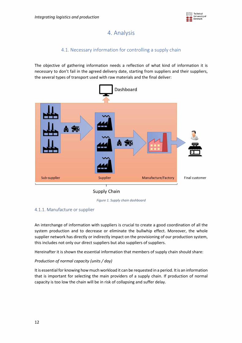
The evolution of raw materials, production, demand and finished goods presented in graphics

tell in a fast way if the data introduced in the initial data will be able to satisfy the customer. It’s

a useful way to present the information fast, easy and intuitively.

The tool can be used also as a monitor at real time. It would help to a manager to react in an

unexpected change in some member of the supply chain. So, if instead of use the simulation

part with random variables the real demand of the month is added, then the closed future can

be predicted and controlled easily.

Figure 12. Image of sub-supplier panel control.


36


37

Figure 13. Image of the whole dashboard


38


39

6. Discussion

Not all products delivered on time pass quality control. As reliability or delivery time, quality is

an important item that point which supplier are most reliable producing raw materials, if the

raw material doesn’t have enough quality implies that the purchase order must be repeated and

the supply chain has lost a valuable time.

Despite quality should be also another KPI included in the model and it’s also an important item

to take it into account, in this project, it has not been included because it would increase the

complexity of calculations. In future researches quality would be an interesting KPI to add into

the model that would approach it to a more real situation.


40

7. Experiment

Hereinafter is going to do a little test to see how a supply chain react in two different scenarios.

It will be interesting see how results and graphics in the dashboard change. In both cases internal

capacities of supply chain and demand won’t variate. What will change will be variation in

random variables generated by excel in the simulation step. It is going to create two different

scenarios in which one will be friendly for the supply chain and the other not:

• Stable or friendly: The priori variation regarding its mean will be a 5%.

Manufacture Supplier Sub-supplier

Demand priori 50 150 1000

σ priori 2,5 7,5 50

Table 6. Priori mean and variance from friendly scenario

• Instable or unfriendly: The priori variation regarding its mean will be 20%.

Manufacture Supplier Sub-supplier

Demand priori 50 150 1000

σ priori 10 30 200

Table 7. Priori mean and variance from unfriendly scenario

Initial data for both cases:

First of all, initial data needs to be add by hand in the excel. The data is the same in both

scenarios. The only thing that change is the simulation demand data. In table 8 and 9, it can be

seen the initial data introduced into manufacture, supplier and sub-supplier:

Table 8. Initial data introduced in manufacture and supplier

200 units/day

50 units

200 units/lot

300 units

20 units

50 units/day

700 DKK

7 DKK

21 DKK

2 DKK

Manufacture

Daily demand


Cost of ownership


Purchase unit cost

Initial data

Production capacity

Order point

Purchase order lot


Security stock

300 units/day

300 units

1000 units/lot

700 units

50 units

150 units/day

700 DKK

7 DKK

21 DKK

2 DKK

Supplier

Initial data

Production capacity

Order point

Purchase order lot


Security stock

Daily demand


Cost of ownership


Purchase unit cost


41

Table 9. Initial data introduced in sub-supplier

Despite mean and variance has been introduced in a fix number in order to generate random

variables, these numbers variate with final results, as it can see in next figures:

Stable:

Table 10. Posteriori mean and variance from friendly scenario.

Instable:

Table 11. Posteriori mean and variance from unfriendly scenario

In figure 14 on next page it can see how purchase order are distributed and planned for the

whole month for a constant demand. The planning starts by manufacture, and then it is followed

by supplier and sub-supplier as it has been explained in chapter 3 (methodology) of this project.

It can see that there is no variation on finished good line in figure 14, so it means that if demand

would remain constant there would not have any delay in delivering a purchase orders.

1600 units/day

1600 units

5000 units/lot

2000 units

100 units

700 DKK

1000 units/day

7 DKK

21 DKK

2 DKK

Sub-supplier

Security stock

Cost of ownership


Initial data

Production capacity

Order point

Purchase order lot


Daily demand


Purchase unit cost

µposteriori 1004,40 µposteriori 148,17 µposteriori 49,37

σposteriori 53,80 σposteriori 6,87 σposteriori 2,08

Normal distributionNormal distributionNormal distribution

µposteriori 962,07 µposteriori 149,83 µposteriori 50,47

σposteriori 194,76 σposteriori 30,47 σposteriori 9,44

Normal distribution Normal distributionNormal distribution


42

Figure 14. Resulting graphics before simulation


43

In figure 15 it can see how a 5% variance respect its demand (or stable scenario) affects to

supply chain. Supply chain can tolerate a small variance of demand without problems in that

case.

Figure 12. Resulting graphics after simulation from stable scenario


44

In figure 16 are graphics of unstable simulation with a 20% variance respect its mean. Like it can

observe in manufacture, in some days of month it starts to have problems with raw materials

stock. These problem with raw materials affect directly to finished goods level, which is not

remain constant like the in other the scenario. Anyway, in that case final product can be

delivered on time because finished goods level never reaches negative number, but maybe with

another variable with the same priori mean and variance, it could be some problems in

delivering on time.


45

Figure 16. Resulting graphics after simulation from instable scenario


46

Table 12. Resulting KPI’s from friendly scenario.

Table 13. Resulting KPI’s from unfriendly scenario.

7 purchases 6 purchases 6 purchases

1400 units 6 purchases 6 purchases

24,68 % 6000 units 30000 units

151 units/day 2,16666667 days 2,50 days

4519 units/month 64,94 % 75,28 %

4200 DKK 105 units/day 396 units/day

0 DKK 3155 units/month 11868 units/month

7700 DKK 25522 DKK 100373 DKK

11900 DKK 0 DKK 0 DKK

16200 DKK 64200 DKK

41722 DKK 164573 DKK

71,4285714 % 50,00 %

7 purchases 3 days

6 purchases 2 days

1400 units

3 days

2 days

Total Cost


Total number of purchase send

Unit purchase number send

Average saturation

Manufacture





Total cost of purchases



Total Cost

Reliability Indicator(*)



Average delivery time(*)

Average saturation




Número total de PO enviadas manu

Total number of units recibidas

Maximum delivery time(*)

Minimum delivery time(*)

Número total de PO recibidas manu

Total number of PO sent subs

Total number of PO received subs

Supplier Sub-supplier





Average saturation






Total Cost





7 purchases 6 purchases 6 purchases

1400 units 6 purchases 6 purchases

25,00 % 6000 units 30000 units

150 units/day 2,5 days 2,67 days

4500 units/month 65,50 % 72,63 %

3843 DKK 104 units/day 438 units/day

0 DKK 3105 units/month 13138 units/month

7700 DKK 27755 DKK 105385 DKK

11543 DKK 0 DKK 0 DKK

16200 DKK 64200 DKK

43955 DKK 169585 DKK

42,8571429 % 33,33 %

7 purchases 3 days

6 purchases 2 days

1400 units

3 days

2 days


Total number of purchase send

Manufacture

Total Cost

Unit purchase number send

Average saturation






Total number of PO sent subs




Total number of PO received subs



Average saturation





Total Cost


Número total de PO recibidas manu


Número total de PO enviadas manu

Total number of units recibidas





Sub-supplierSupplier




Total Cost






Average saturation


47

As table 12 and 13 show, variation on demand greatly affects on supply chain and KPI’s of each

of its participants. When bigger is instability of demand, more all supply chain is delayed in its

deliveries, it also gets a worse are the results in terms of reliability and average delivery time.

Saturation level is a KPI that, in that case it’s not very relevant, because normal distribution of

variables makes it constant in both scenarios.

A curious data is that cost indicator in manufacture is cheaper in instable scenario. It can be

explained because, at some point of month the stock level of finished goods is reduced and,

consequently, it reduces the cost of stock possession.

Finally, in both cases manufacture can produce its demand without problems, but an increase

of variation in demand would affect negatively into the whole supply chain.


48

8. Conclusions

That project has developed a dashboard for a supply chain in order to help a supply chain

manager to get a complete overview about the status of its chain. The reason to do a dashboard

is to make decision making easier. The method used for developing it has been to create a

common purchase planning for the whole chain using an order point policy. Then a simulation

for a real case has been added into that dashboard.

Finally this dashboard has been tested with a little experiment that has shown the behaviour of

the supply chain in two different scenarios of different demands.

To sum up it can be said that the dashboard that has been developed in that project is very

limited and cannot be applied in many real circumstances.

First of all, transport is not taken it into account in delivery time, and it is normally one of the

main factors that affects.

Another limitation is that it is considered one raw material to produce just one final product,

when normally this relation is many to one or one to many. Usually in order to produce a unit of

product it is necessary many different kinds of raw materials, which makes the problem bigger

and more complex for a supply chain manager.

Demand is not something that should follow any kind of behaviour and it can be very random,

which is something very common in a real case. This dashboard just considers an stable demand

and doesn’t tolerate very well large variation in a simulation case.

This dashboard has demonstrated be very demanding with every member of supply chain and a

good tool to detect problems before they occur. It’s is also very useful to evaluate every member

in a quantitative way.

It has also demonstrated be very intuitive and easy to use for a user.


49

9. Bibliography

A. Kubde, R. (2012). Collaborative Planning, Forecasting and Replenishment: Determinants of

Joint Action in Buyer-supplier Relationships. Research Journal of Business Management.

https://doi.org/10.3923/rjbm.2012.12.18

Al-Saad, B. B., Murray, P. A. P. A., Vanderhaeghen, M. M., Yannlmaras, D. D., & Naime, R. K. R.

K. (2014). Development and implementation of the AVAILS + collaborative forecasting

tool for production assurance in the Kuwait oil company, North Kuwait. SPE Economics

and Management, 6(4), 191–198. Retrieved from

http://www.scopus.com/inward/record.url?partnerID=HzOxMe3b&scp=84908702630&o

rigin=inward

Anand, R. (2010). Monitor and optimize machine efficiency with OEE dashboards. SAE

Technical Papers. https://doi.org/10.4271/2010-01-0398

Bai, C., & Sarkis, J. (2014). Determining and applying sustainable supplier key performance

indicators. Supply Chain Management: An International Journal, 19(3), 275–291.

https://doi.org/10.1108/SCM-12-2013-0441

Bubel, D. (2017). Implementation of the principles of the process orientation in the aspect of

logistic management of supply chain. In Communication, Management and Information

Technology - Proceedings of the International Conference on Communication,

Management and Information Technology, ICCMIT 2016 (pp. 717–723). Retrieved from

https://www.scopus.com/inward/record.uri?eid=2-s2.0-

85017010984&partnerID=40&md5=70a20891a5d54fee2c4b85253325442e

Chyr, F., Lin, T. M., & Ho, C. F. (1990). Comparison between just-in-time and EOQ system.

Engineering Costs and Production Economics, 18(3), 233–240.

https://doi.org/10.1016/0167-188X(90)90125-2

Cobb, B. R., & Johnson, A. W. (2014). A note on supply chain coordination for joint

determination of order quantity and reorder point using a credit option. European

Journal of Operational Research, 233(3), 790–794.

https://doi.org/10.1016/j.ejor.2013.10.009

Drawert, S. (n.d.). Corporate Performance Management in Logistics and Procurement –

Focused Identification of Weak Points with Supply Chain Controlling Why Does Logistics

Need Supply Chain Controlling ?

El Farouk Imane, I., Foaud, J., & Abdennebi, T. (2017). From modeling to logistic KPI Use of

SCOR model and ARIS to build a dashbord to manage medicines supply chain in moroccan

public hospital. Colloquium in Information Science and Technology, CIST, 746–750.

https://doi.org/10.1109/CIST.2016.7804986

Federgruen, A., & Zheng, Y.-S. (1992). An Efficient Algorithm for Computing an Optimal (r, Q)

Policy in Continuous Review Stochastic Inventory Systems. Operations Research, 40(4),

808–813. https://doi.org/10.1287/opre.40.4.808

Franceschini, F., & Turina, E. (2012). Proposal for a Performance Dashboard for the Monitoring

of Water and Sewage Service Companies (WaSCs). Water Resources Management, 26(1),


50

63–80. https://doi.org/10.1007/s11269-011-9901-3

Goh, R. S. M., Wang, Z., Yin, X., Fu, X., Ponnambalam, L., Lu, S., & Li, X. (2013). RiskVis: Supply

chain visualization with risk management and real-time monitoring. IEEE International

Conference on Automation Science and Engineering, 207–212.

https://doi.org/10.1109/CoASE.2013.6653910

Jahnukainen, J., & Lahti, M. (1999). Efficient purchasing in make-to-order supply chains.

International Journal of Production Economics, 59(1), 103–111.

https://doi.org/10.1016/S0925-5273(98)00231-X

Ji, Z. G., & Liu, L. X. (2010). The Application of CPFR Model in Information System. Advanced

Materials Research, 129–131, 652–657.

https://doi.org/10.4028/www.scientific.net/AMR.129-131.652

Kang, J., & Kim, Y. (2010). Inventory replenishment and delivery planning in a two-level supply

chain with compound Poisson demands, 1107–1118. https://doi.org/10.1007/s00170-

009-2468-y

Karr, B. (2012). Taking dashboards out of wonderland. Industrial Engineer, 44(9), 32–36.

Kreng, V. B., & Chen, F. (2017). Three echelon buyer--supplier delivery policy — a supply chain

collaboration approach Three echelon buyer – supplier delivery policy — a supply chain

collaboration approach, 7287(May). https://doi.org/10.1080/09537280701302631

Li, Z. P. ., Lim, L. H. ., Chen, X. S. ., & Tan, C. S. . (2016). Supplier selection decision-making in

supply chain risk scenario using agent based simulation. IEEE International Conference on

Industrial Engineering and Engineering Management, 2016–Janua, 900–904.

https://doi.org/10.1109/IEEM.2015.7385778

Lin, J. T., Chang, P., Chen, J.-H., & Xin, W.-X. (2003). KPI with Data Flow Analysis for CPFR: A

CMC Case Study. International Journal of Electronic Business Management, 1(2/3), 110–

119. Retrieved from

http://www.doaj.org/doaj?func=openurl&issn=17282047&date=2003&volume=1&issue=

2/3&spage=110&genre=article

Lin, Y. C. E. (2006). Implementation of Supply Chain Logistics Process Reengineering and E-

Business Solution for a Chain Store Business. International Journal 01 Electronic Business

Management, 4(5), 357–367.

Min, W., & Sui Pheng, L. (2005). Economic order quantity (EOQ) versus just-in-time (JIT)

purchasing: an alternative analysis in the ready-mixed concrete industry. Construction

Management and Economics, 23(4), 409–422.

https://doi.org/10.1080/01446190500041339

Pal, P., & Kumar, B. (2008). “16T”: toward a dynamic vendor evaluation model in integrated

SCM processes. Supply Chain Management: An International Journal, 13(6), 391–397.

https://doi.org/10.1108/13598540810905642

Porras, E., & Dekker, R. (2008). An inventory control system for spare parts at a refinery: An

empirical comparison of different re-order point methods. European Journal of

Operational Research, 184(1), 101–132. https://doi.org/10.1016/j.ejor.2006.11.008

Pradhan, S. K., & Routroy, S. (2014). Analyzing the performance of supplier development: a

case study. International Journal of Productivity and Performance Management, 63(2),

209–233. https://doi.org/10.1108/IJPPM-09-2012-0106


51

Pretorius, C., Ruthven, G. A., & Von Leipzig, K. (2013). An empirical supply chain measurement

model for a national egg producer based on the supply chain operations reference

model. Journal of Transport and Supply Chain Management, 7(1), 1–13.

https://doi.org/10.4102/jtscm.v7i1.97

R.A. Kubde and S.V. Bansod, 2010. Collaborative Planning Forecasting and Replenishment

Initiatives: A State of Art. Asian Journal of Industrial Engineering, 2: 89-104.

Raghavan, N. R. S. (2002). Stochastic models for analysis of supply chain networks.

Rau, H., & OuYang, B. C. (2008). An optimal batch size for integrated production-inventory

policy in a supply chain. European Journal of Operational Research, 185(2), 619–634.

https://doi.org/10.1016/j.ejor.2007.01.017

Schneider, H. (1978). Methods for Determining the Re-order Point of an (s, S) Ordering Policy

when a Service Level is Specified. The Journal of the Operational Research Society, 29(12),

1181-1193. doi:10.2307/3009583

Sithole, B., Silva, S. G., & Kavelj, M. (2016). Supply chain optimization: Enhancing end-to-end

visibility. Procedia Engineering, 159(June), 12–18.

https://doi.org/10.1016/j.proeng.2016.08.058

Strandhagen, J. O., & Dreyer, H. (2006). Supply Chain Control Dashboards, 1–19.

Wu, M. (2007). Using Matlab to Compute the Break-even Point in Supply Chain Management,

(66).

Xia, L. X. X., & Lim, R. (2008). Supplier performance measurement in a supply chain. 2008 6th

IEEE International Conference on Industrial Informatics, 877–881.

https://doi.org/10.1109/INDIN.2008.4618224

Yang, P. C., Wee, H. M., & Yang, H. J. (2007). Global optimal policy for vendor-buyer integrated

inventory system within just in time environment. Journal of Global Optimization, 37(4),

505–511. https://doi.org/10.1007/s10898-006-9058-4

Ying, L., Lijun, X., & Wei, S. (2009). Designing supply chain KPIs for upper-level management.

Proceedings - 2009 IITA International Conference on Services Science, Management and

Engineering, SSME 2009, 19–21. https://doi.org/10.1109/SSME.2009.139

Zimmer, K. (2002). Supply chain coordination with uncertain just-in-time delivery. International

Journal of Production Economics, 77(1), 1–15. https://doi.org/10.1016/S0925-

5273(01)00207-9

52

10. Acknowledgments

I really would like to thank to professor Peter Jacobsen, who is my tutor and has been my guide

during last months, to develop this project. He has helped me and has contributed to realize this

project.

I would also like to thank Gema Sánchez to help me in checking and correcting some language

mistakes in the report.

integrating logistics and production

Documents