integer ratios of factorials, hypergeometric functions...
TRANSCRIPT

Integer ratios of factorials, hypergeometric functions, andrelated step functions
by
Jonathan William Bober
A dissertation submitted in partial fulfillmentof the requirements for the degree of
Doctor of Philosophy(Mathematics)
in The University of Michigan2009
Doctoral Committee:
Professor Jeffrey C. Lagarias, ChairProfessor Douglas O. RichstoneProfessor Karen E. SmithAssistant Professor Djordje MilicevicProfessor Kannan Soundararajan, Stanford University

c© Jonathan William Bober2009

ACKNOWLEDGEMENTS
The math department at the University of Michigan has been a wonderful place
to spend five years, in no small part because of the many great friends and colleagues
I have had during my time here.
I would like to thank my committee for taking the time to read my thesis. In
particular, the introduction was greatly improved from some input from Karen Smith,
and none of this would have been written if not for Jeff Lagarias. Jeff suggested the
work that led to this thesis and has constantly pushed me to improve everything
about it, and it has been a pleasure learning from him.
Theorem 1.1 appears in [8], and I would like to thank the anonymous referee of that
paper for many helpful comments. Theorem 1.2 is joint work with Jason P. Bell, and
appears in [5]. Also, the results of Theorem 1.2 were considerably strengthened with
help from Kannan Soundararajan. Theorem 1.2 was also proved by Enrico Bombieri
and Jean Bourgain [10] through different methods, and I would like to thank Bombieri
for providing his notes. I also thank Alexander Borisov for providing a preprint of
[12].
This work was partially supported by the NSF RTG grant DMS-0502170 and the
NSF grant DMS-0500555.
ii

TABLE OF CONTENTS
ACKNOWLEDGEMENTS . . . . . . . . . . . . . . . . . . . . . . . . . . ii
LIST OF TABLES . . . . . . . . . . . . . . . . . . . . . . . . . . . . . . . . v
CHAPTER
1. Background and results . . . . . . . . . . . . . . . . . . . . . . . 1
1.1 Introduction . . . . . . . . . . . . . . . . . . . . . . . . . . . 11.2 Statement of results . . . . . . . . . . . . . . . . . . . . . . . 41.3 Applications to the classification of cyclic quotient singularities 71.4 The Beurling–Nyman criterion for the Riemann Hypothesis . 8
2. The connection between factorial ratios and step functions . 12
2.1 Restatements of main theorems . . . . . . . . . . . . . . . . . 122.2 Equivalence of the restated theorems . . . . . . . . . . . . . . 152.3 G-functions and the balancing condition . . . . . . . . . . . . 19
3. Factorial ratios of height 1 . . . . . . . . . . . . . . . . . . . . . . 22
3.1 Introduction . . . . . . . . . . . . . . . . . . . . . . . . . . . 223.1.1 Notation . . . . . . . . . . . . . . . . . . . . . . . . 23
3.2 Connection between factorial ratios and hypergeometric series 243.3 A Classification of Integral Factorial Ratios . . . . . . . . . . 30
3.3.1 Monodromy for Hypergeometric Functions nFn−1 . . 303.3.2 The Classification . . . . . . . . . . . . . . . . . . . 33
3.4 A Listing of all Integral Factorial Ratios with L−K = 1 . . . 38
4. Proof of Theorem 1.2 . . . . . . . . . . . . . . . . . . . . . . . . . 43
4.1 Introduction . . . . . . . . . . . . . . . . . . . . . . . . . . . 434.1.1 Notation . . . . . . . . . . . . . . . . . . . . . . . . 45
4.2 An explicit lower bound for the L2 norm . . . . . . . . . . . . 454.3 Explicit bounds and remarks . . . . . . . . . . . . . . . . . . 50
iii

5. Proof of Theorem 1.3 . . . . . . . . . . . . . . . . . . . . . . . . . 52
BIBLIOGRAPHY . . . . . . . . . . . . . . . . . . . . . . . . . . . . . . . . 55
iv

LIST OF TABLES
Table
3.1 The three infinite families of integral factorial ratio sequences . . . . 393.2 The 52 sporadic integral factorial ratio sequences . . . . . . . . . . . 39
v

CHAPTER 1
Background and results
1.1 Introduction
Fix two sets of natural numbers a = (a1, a2, . . . , aK) and b = (b1, b2, . . . , bL). We
consider the factorial ratio sequence
un(a,b) =(a1n)!(a2n)! · · · (aKn)!
(b1n)!(b2n)! · · · (bLn)!. (1.1)
Our main question is: For which a and b is un(a,b) an integer for all n ≥ 0? Nearly
always we require thatK∑k=1
ak =L∑l=1
bl, (1.2)
and we will call a sequence satisfying this condition balanced. This condition ensures
that both un and its inverse grow at most exponentially, instead of factorially.
The simplest examples of balanced integer factorial ratio sequences come from
binomial coefficients: for any a ≥ b ≥ 0 we have the sequence
un(a; b, a− b) =
(an
bn
)=
(an)!
(bn)!((a− b)n)!.
Another example, which was given by Catalan in 1874 [15], is
(2a)!(2b)!
a!b!(a+ b)!,
which is also an integer for all integers a, b. (We obtain an integer factorial ratio
sequence by setting a = a′n and b = b′n for some integers a′ and b′.) If un(a,b)
is balanced and is always an integer, then necessarily L ≥ K, with L = K only
in the case that un(a,b) = 1 for all n, and we shall call the parameter L − K the
1
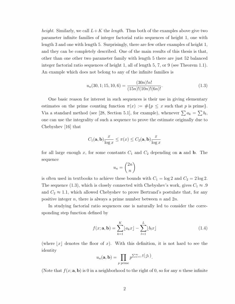
height. Similarly, we call L+K the length. Thus both of the examples above give two
parameter infinite families of integer factorial ratio sequences of height 1, one with
length 3 and one with length 5. Surprisingly, there are few other examples of height 1,
and they can be completely described. One of the main results of this thesis is that,
other than one other two parameter family with length 5 there are just 52 balanced
integer factorial ratio sequences of height 1, all of length 5, 7, or 9 (see Theorem 1.1).
An example which does not belong to any of the infinite families is
un(30, 1; 15, 10, 6) =(30n)!n!
(15n)!(10n)!(6n)!. (1.3)
One basic reason for interest in such sequences is their use in giving elementary
estimates on the prime counting function π(x) := #{p ≤ x such that p is prime}.Via a standard method (see [28, Section 5.1], for example), whenever
∑ak =
∑bl,
one can use the integrality of such a sequence to prove the estimate originally due to
Chebyshev [16] that
C1(a,b)x
log x≤ π(x) ≤ C2(a,b)
x
log x
for all large enough x, for some constants C1 and C2 depending on a and b. The
sequence
un =
(2n
n
)is often used in textbooks to achieve these bounds with C1 = log 2 and C2 = 2 log 2.
The sequence (1.3), which is closely connected with Chebyshev’s work, gives C1 ≈ .9
and C2 ≈ 1.1, which allowed Chebyshev to prove Bertrand’s postulate that, for any
positive integer n, there is always a prime number between n and 2n.
In studying factorial ratio sequences one is naturally led to consider the corre-
sponding step function defined by
f(x; a,b) =K∑k=1
bakxc −L∑l=1
bblxc (1.4)
(where bxc denotes the floor of x). With this definition, it is not hard to see the
identity
un(a,b) =∏
p prime
pP∞α=1 f( n
pα ).
(Note that f(x; a,b) is 0 in a neighborhood to the right of 0, so for any n these infinite
2

sums and this infinite product are actually finite.) In 1918 Landau [20] proved that
un(a,b) is an integer for all n if and only of f(x; a,b) is nonnegative for all x > 0
(see Theorem 2.1). Thus, classifying integer factorial ratios of the form (1.1) is the
same as classifying step functions of the form (1.4).
Functions of the form (1.4) have a more direct connection to the distribution of
prime numbers through the Beurling–Nyman criterion for the Riemann Hypothesis.
Loosely speaking, the Beurling–Nyman criterion is the statement that the Riemann
Hypothesis is true if and only if the constant function call be well-approximated by
functions that look like (1.4). (This is discussed in more detaio in Section 1.4.)
With this in mind, V. I. Vasyunin [31] studied the classification of such functions
which take only the values 0 and 1. Based on extensive computation, he gave a con-
jectural classification which our Theorem 1.1 proves: there are three infinite families
and 52 more functions which do not fall into these families. In Chapter 2 we will
show how Vasyunin’s conjecture is equivalent to our Theorem 1.1.
One curious consequence of Theorem 1.1 is that the number of terms in such a
function must be less than or equal to 9 if it is to take on only the values 0 and 1;
that is, if
f(x) =K∑k=1
bakxc −K+1∑l=1
bblxc
with∑ak =
∑bj, ak 6= bl for all k, l and ak, bl 6= 0, and K > 4, then f(x) < 0
for some x. It would be nice to have a more direct proof of this statement, but the
only proof that will be presented here is one where we simply write down all of the
possibilities and notice that none of them has more than nine terms.
Our second theorem is a generalization of this phenomenon, and answers a con-
jecture of A. Borisov related to cyclic quotient singularities [12, Conjecture 4]. We
will prove that, subject to the obvious nondegeneracy conditions, if L + K is large
enough (as compared to L−K) then
f(x; a,b) =K∑k=1
bakxc −L∑l=1
bblxc
cannot be always nonnegative. In terms of factorial ratio sequences, this says that a
balanced sequence of large length must have sufficiently large height if it is to have a
chance of being integral. In the specific case of height 1, the bounds that we achieve
by this method will be quite far from what is true, however.
Finally, we may turn our attention to whether there exist classifications similar to
3

that of Theorem 1.1 for integer factorial ratio sequences with fixed D = L−K > 1.
Our Theorem 1.3 says that for fixed K and L, if we require that∑ak =
∑bl then
un(a,b) =(a1n)!(a2n)! · · · (aKn)!
(b1n)!(b2n)! · · · (bLn)!
is an integer for all n if and only if a and b have nonnegative integer coordinates and
lie in a set W which is a finite union of subspaces of RK+L. Combining this with
Theorem 1.2, we find that there exists a finite classification for any fixed height, of
which Theorem 1.1 is just one example.
1.2 Statement of results
Our first theorem, which is proved in Chapter 3, describes completely the classi-
fication of integral factorial ratios of the form
un(a,b) =(a1n)!(a2n)! · · · (aKn)!
(b1n)!(b2n)! · · · (bK+1n)!
such that∑ak =
∑bj. As is explained in Chapter 2, this proves a conjecture of
Vasyunin [31] concerning the classification of functions of the form
f(x; a,b) =K∑k=1
bakxc −L∑l=1
bblxc
which take only the values 0 and 1. We will not use the connection with step functions
to prove this theorem, however, but will instead use a connection with hypergeometric
series.
The generating function
u(z) =∞∑n=0
un(a,b)zn
is a hypergeometric series, and when un(a,b) is balanced, so that∑ak =
∑bl, we
show that it is in fact what is known as a G-function (see Section 2.3). Moreover,
F. Rodriguez-Villegas [25] noticed that u(z) is algebraic if and only if L − K = 1,∑ak =
∑bl, and un(a,b) is an integer for all n. Combining this with work of
Beukers and Heckman [6] which classifies all algebraic hypergeometric series of the
form that we are interested in, we will be able to prove the following.
4
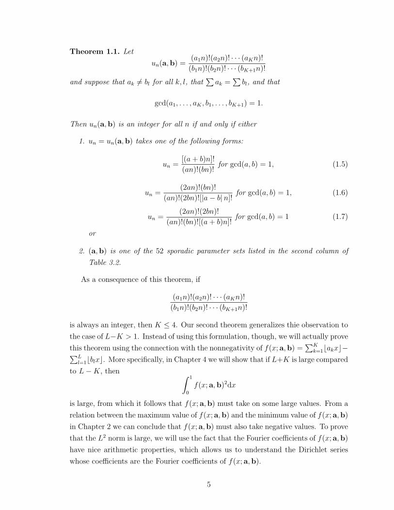
Theorem 1.1. Let
un(a,b) =(a1n)!(a2n)! · · · (aKn)!
(b1n)!(b2n)! · · · (bK+1n)!
and suppose that ak 6= bl for all k, l, that∑ak =
∑bl, and that
gcd(a1, . . . , aK , b1, . . . , bK+1) = 1.
Then un(a,b) is an integer for all n if and only if either
1. un = un(a,b) takes one of the following forms:
un =[(a+ b)n]!
(an)!(bn)!for gcd(a, b) = 1, (1.5)
un =(2an)!(bn)!
(an)!(2bn)![|a− b|n]!for gcd(a, b) = 1, (1.6)
un =(2an)!(2bn)!
(an)!(bn)![(a+ b)n]!for gcd(a, b) = 1 (1.7)
or
2. (a,b) is one of the 52 sporadic parameter sets listed in the second column of
Table 3.2.
As a consequence of this theorem, if
(a1n)!(a2n)! · · · (aKn)!
(b1n)!(b2n)! · · · (bK+1n)!
is always an integer, then K ≤ 4. Our second theorem generalizes thie observation to
the case of L−K > 1. Instead of using this formulation, though, we will actually prove
this theorem using the connection with the nonnegativity of f(x; a,b) =∑K
k=1bakxc−∑Ll=1bblxc. More specifically, in Chapter 4 we will show that if L+K is large compared
to L−K, then ∫ 1
0
f(x; a,b)2dx
is large, from which it follows that f(x; a,b) must take on some large values. From a
relation between the maximum value of f(x; a,b) and the minimum value of f(x; a,b)
in Chapter 2 we can conclude that f(x; a,b) must also take negative values. To prove
that the L2 norm is large, we will use the fact that the Fourier coefficients of f(x; a,b)
have nice arithmetic properties, which allows us to understand the Dirichlet series
whose coefficients are the Fourier coefficients of f(x; a,b).
5
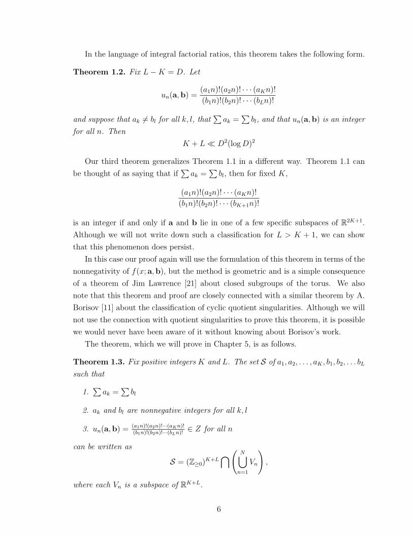
In the language of integral factorial ratios, this theorem takes the following form.
Theorem 1.2. Fix L−K = D. Let
un(a,b) =(a1n)!(a2n)! · · · (aKn)!
(b1n)!(b2n)! · · · (bLn)!
and suppose that ak 6= bl for all k, l, that∑ak =
∑bl, and that un(a,b) is an integer
for all n. Then
K + L� D2(logD)2
Our third theorem generalizes Theorem 1.1 in a different way. Theorem 1.1 can
be thought of as saying that if∑ak =
∑bl, then for fixed K,
(a1n)!(a2n)! · · · (aKn)!
(b1n)!(b2n)! · · · (bK+1n)!
is an integer if and only if a and b lie in one of a few specific subspaces of R2K+1.
Although we will not write down such a classification for L > K + 1, we can show
that this phenomenon does persist.
In this case our proof again will use the formulation of this theorem in terms of the
nonnegativity of f(x; a,b), but the method is geometric and is a simple consequence
of a theorem of Jim Lawrence [21] about closed subgroups of the torus. We also
note that this theorem and proof are closely connected with a similar theorem by A.
Borisov [11] about the classification of cyclic quotient singularities. Although we will
not use the connection with quotient singularities to prove this theorem, it is possible
we would never have been aware of it without knowing about Borisov’s work.
The theorem, which we will prove in Chapter 5, is as follows.
Theorem 1.3. Fix positive integers K and L. The set S of a1, a2, . . . , aK , b1, b2, . . . bL
such that
1.∑ak =
∑bl
2. ak and bl are nonnegative integers for all k, l
3. un(a,b) = (a1n)!(a2n)!···(aKn)!(b1n)!(b2n)!···(bLn)!
∈ Z for all n
can be written as
S = (Z≥0)K+L
⋂(N⋃n=1
Vn
),
where each Vn is a subspace of RK+L.
6

In Chapter 2 we will make more precise the connection between the factorial ratio
sequence un(a,b) and the step function f(x; a,b) and we will restate these theorems
in terms of the classification of nonnegative f(x; a,b). (To distinguish, the versions
of these theorems in terms of step functions will be labeled Theorems 1.1*, 1.2*
and 1.3*.) Additionally, in the next section we point out some applications to the
classification of quotient singularities due to Alexander Borisov.
1.3 Applications to the classification of cyclic quotient singularities
By work of Alexander Borisov [12], our theorems have applications to the work
of cyclic quotient singularities. We defer to [12] for details, but state here Borisov’s
theorem which makes the connection, and some consequences.
Theorem 1.4 (A. Borisov, [12, Theorem 11]). Suppose u1, u2, . . . , uk and v1, v2, . . . , vk
are two finite sets of linear forms on Rd with coefficients in N. Suppose further that∑Kk=1 ui(X) =
∑Ll=1 vl(X) for all X = (x1, . . . , xd) ∈ Rd. Then the following two
statements are equivalent.
1. For every X = (x1, . . . , xd) ∈ Nd,∏Kk=1 uk(X)!∏Ll=1 vl(X)!
∈ N.
2. For any n ∈ N and all X = (x1, . . . , xd) ∈ Zd such that all{ui(X)n
}and
{vi(X)n
}are nonzero, the following point in Tn+k defines a Gorenstein cyclic quotient
with Shokurov minimal log-discrepancy at least K:({−u1(X)
n
},{−u2(X)
n
}, · · · ,
{−uK(X)
n
},{v1(X)n
},{v2(X)n
}, · · · ,
{vL(X)n
}).
Through this connection Theorem 1.1 establishes a new proof of a classification of
terminal cyclic quotient singularities in dimension 4 which was conjectured by Mori,
Morrison, and Morrison [23] and first proved by Sankaran [27]. Additionally, Theorem
1.1 implies the following in higher dimensions.
Proposition 1.5. Suppose d ≥ 5 and we have a one-parameter family of Gorenstein
cyclic quotient singularities of dimension 2d+1 with Shukarov minimal log-discrepancy
d. Then up to the permutation of the coordinates in the T (2d+1), the corresponding
points lie in the subtorus x1 + x2 = 1.
7

Proof. See [12, Conjecture 1].
Additionally, Borisov notes that Theorem 1.2* is equivalent to the following.
Proposition 1.6. Suppose a ≥ 0 is any real number. Then for all large enough
d ∈ N, for all but finitely many (x1, x2, . . . , xd) ∈ T d that define a cyclic quotient
singularity with Shokurov minimal log-discrepancy at least d/2 − a, for some pair of
indices 1 ≤ i < j ≤ d we have xi + xj = 1.
Proof. See [12, Conjecture 3].
1.4 The Beurling–Nyman criterion for the Riemann Hypothesis
The Riemann ζ-function ζ(s), where s = σ + it, is classically defined in the half
plane σ > 1 by the Dirichlet series
ζ(s) =∞∑n=1
1
ns.
One way to obtain an analytic continuation of ζ(s) to the half plane σ > 0 is by
writing this Dirichlet series as a Riemann–Stiltjes integral and integrating by parts.
Doing so, we have
ζ(s) =
∫ ∞1−
y−sdbyc
= s
∫ ∞1
y−s−1byc dy.
Writing byc = y −{y}, we obtain
ζ(s)
s=
∫ ∞1
1
ysdy −
∫ ∞1
{y}ys+1
dy
=1
s− 1−∫ ∞
1
{y}ys+1
dy.
Since the integral∫∞
1{y}ys+1 dy converges absolutely for σ > 0, this expression gives an
analytic continuation of the ζ-function to this region, with the exception of a simple
pole at s = 1.
Additionally, this expression indicates a relation between the functions {x} and
8

ζ(s). In fact, if we instead start with
αsζ(s) =
∫ ∞1−
(α
y
)sdbyc =
∫ ∞1−
y−sdbαyc,
which is valid for 0 ≤ α ≤ 1, and perform the same calculation, we find that
αsζ(s)
s=
α
s− 1−∫ ∞
1
{αy}ys+1
dy.
Now suppose that f(x) is a function of the form
f(x) =N∑n=1
cnbαnxc ,
where∑N
n=1 cnαn = 0. Using the relation bxc = x−{x}, we may rewrite this as
f(x) = −N∑n=1
cn{αnx} ,
and thus ∫ ∞1
f(y)
ys+1dy =
ζ(s)
s
N∑n=1
cnαsn.
We will now see how the approximation of 1 by f(x) leads to information about the
zeros of ζ(s). Consider
∫ ∞1
(1− f(y))
y
1
ysdy =
1
s
(1− ζ(s)
N∑n=1
cnαsn
). (1.8)
By Holder’s inequality, for σ > (p− 1)/p we have
∫ ∞1
∣∣∣∣(1− f(y))
y
1
ys
∣∣∣∣ dy ≤ (∫ ∞1
∣∣∣∣1− f(y)
y
∣∣∣∣p dy
)1/p(∫ ∞1
1
yσp/(p−1)dy
)(p−1)/p
=
(∫ ∞1
∣∣∣∣1− f(y)
y
∣∣∣∣p dy
)1/p(p− 1
σp− p+ 1
)(p−1)/p
.
Let(∫∞
1
∣∣∣1−f(y)y
∣∣∣p dy)1/p
= ε. We then have
∣∣∣∣∣1− ζ(s)N∑n=1
cnαsn
∣∣∣∣∣p/(p−1)
≤ εp/(p−1) |s|p/(p−1) p− 1
σp− p+ 1.
9

Thus ζ(s) 6= 0 whenever the right hand side is smaller than 1 and σ > (p− 1)/p. For
fixed s, the right hand side goes to 0 as ε → 0, so this proves half of the following
theorem.
Proposition 1.7 (Nyman, Beurling). ζ(s) has no zeros in the half plane σ > p−1p
if
and only if for any ε > 0 there exists a function f(x) of the form
f(x) =N∑n=1
cnbαnxc (1.9)
with∑cnαn = 0 and 0 ≤ αn ≤ 1 for all n such that
(∫ ∞1
∣∣∣∣1− f(x)
x
∣∣∣∣p dx
)1/p
< ε.
Remark 1.8. This theorem appears for p = 2 in a different form in Nyman’s thesis
[24]. Beurling gives the generalization to p > 2 in [7]. Both Beurling and Nyman
work instead with the function space Lp((0, 1), dx), however. Here we are essentially
considering Lp((1,∞), dxx
), which corresponds to the change of variable x ←→ 1/x.
Also, Beurling and Nyman in fact show that ζ(s) being zero-free for σ > p−1p
is
equivalent to functions of the form (1.9) being dense in Lp((1,∞), dxx
).
The argument above suggests a candidate for a function f(x) that we might try to
use to approximate 1. From equation (1.8) we see that we might want to try choosing
f(x) =∑N
n=1 cnbαnxc so that∑N
n=1 cnαs ≈ 1/ζ(s). For σ > 1, (and for σ > 1/2 if
we assume the Riemann Hypothesis), 1/ζ(s) =∑∞
n=1 µ(n)/ns, so it seems we should
choose cn = µ(n) and αn = 1/n.
In fact, for any fixed x, we have
∞∑n=1
µ(n)⌊xn
⌋= 1. (1.10)
However, there is no N for which the finite sum∑N
n=1µ(n)n
is 0, so we can not just
take partial sums of this series. There are other candidates we may consider, though.
For example, one possibility is to take a partial sum of the series∑∞
n=1 µ(n)⌊xn
⌋and
add in a correction factor at the n + 1-st place so that the condition∑cnαn = 0 is
satisfied. The sequence of functions we get is
fn(x) =N∑n=1
µ(n)⌊xn
⌋−N
(N∑n=1
µ(n)
n
)⌊xn
⌋.
10

This sequence converges to 1 pointwise, but not in L2((1,∞), dxx
) (see [2]). Neverthe-
less, as is perhaps suggested by (1.10), it is possible to restrict to αn = 1n
and get a
theorem of the same type.
Proposition 1.9 (Baez-Duarte [3]). The Riemann Hypothesis is true if and only if
for every ε > 0 there is a function
f(x) =N∑n=1
cn
⌊xn
⌋(1.11)
such that ∫ ∞1
∣∣∣∣1− f(x)
x
∣∣∣∣2 dx < ε.
Although Baez-Duarte had not yet proven this theorem, its conjectural existence
was motivation for Vasyunin [31] to study functions of the form (1.11) taking only
the values 0 and 1.
There is one more aspect of this approach that we should mention, though we
will not use it. From the equation (1.8), we see that there is a relationship between
approximating the constant function with linear combinations of floor functions and
approximating the inverse of the zeta function. In fact, an “equivalent” formulation
of the Beurling–Nyman criterion is the statement that the Riemann Hypothesis is
true if and only if
limN→∞
infDN
∫ ∞−∞
(1− ζ(1/2 + it)DN(1/2 + it)
1/2 + it
)2
dt = 0,
where DN ranges over all generalized Dirichlet polynomials of length N . (See [4].)
For more on the Beurling–Nyman criterion, one can also see the paper of Burnol
[13], which proves Baez-Duarte’s theorem from a more complex-analytic viewpoint,
and the paper of Balazard and Saias [4], which proves the Beurling–Nyman criterion
by using the theory of the Hardy space of the half plane σ > 1/2 and its relation to
L2((0, 1)) through the Mellin transform.
11

CHAPTER 2
The connection between factorial ratios and step functions
2.1 Restatements of main theorems
The main object of this chapter is to prove the equivalence of Theorems 1.1, 1.2,
1.3 and the following restatements of those theorems in terms of step functions related
to the Beurling-Nyman criterion.
Our first theorem was conjectured by Vasyunin [31] and is a complete description
of functions of the form
f(x) =N∑k=1
⌊x
mk
⌋−
2N+1∑k=N+1
⌊x
mk
⌋,
with mk > 0 for all k such that f(x) takes only the values 0 and 1. Equivalently,
through a change of variables, this is a description of functions of the form
f(x; a,b) =K∑k=1
bakxc −L∑l=1
bblxc
which take only the values 0 and 1.
Theorem 1.1*. Let
f(x) =N∑k=1
⌊x
mk
⌋−
2N+1∑k=N+1
⌊x
mk
⌋,
with mk > 0 for all k, and suppose that mi 6= mj for all i ≤ N, j ≤ N + 1, and that
gcd(m1,m2, . . . ,m2N+1) = 1.
Then f(x) takes only the values 0 and 1 if and only if either
12

1. f(x) takes one of the following forms:
f(x) =⌊ xab
⌋−⌊
x
b(a+ b)
⌋−⌊
x
a(a+ b)
⌋where gcd(a, b) = 1, (2.1)
f(x) =
⌊x
b(a− b)
⌋+
⌊x
2a(a− b)
⌋−⌊
x
2b(a− b)
⌋−⌊
x
a(a− b)
⌋−⌊ x
2ab
⌋(2.2)
where
gcd(a, b) = gcd(2, a− b) = 1 and a > b > 0,
f(x) =
⌊x
12b(a− b)
⌋+
⌊x
a(a− b)
⌋−⌊
x
b(a− b)
⌋−⌊
x12a(a− b)
⌋−⌊ xab
⌋(2.3)
where
gcd(a, b) = gcd(2, a) = gcd(2, b) = 1 and a > b > 0,
f(x) =
⌊x
b(a+ b)
⌋+
⌊x
a(a+ b)
⌋−⌊
x
2b(a+ b)
⌋−⌊
x
2a(a+ b)
⌋−⌊ x
2ab
⌋(2.4)
where
gcd(a, b) = gcd(2, a+ b) = 1,
f(x) =
⌊x
12b(a+ b)
⌋+
⌊x
12a(a+ b)
⌋−⌊
x
b(a+ b)
⌋−⌊
x
a(a+ b)
⌋−⌊ xab
⌋(2.5)
where
gcd(a, b) = gcd(2, a) = gcd(2, b) = 1,
or
2. f(x) is one of the 52 sporadic step functions given by
(m1,m2, . . . ,mN) =
(M
a1
,M
a2
, . . . ,M
aN
)and
(mN+1,mN+2, . . . ,m2N+1) =
(M
b1,M
b2, . . . ,
M
bN+1
)for some a (or permutation of a) and b (or permutation of b) listed in the
second column of Table 3.2, where
M = lcm(a1, a2, . . . , aN , b1, b2, . . . bN+1).
13

As a consequence of Theorem 1.1*, if
f(x; a,b) =K∑k=1
bakxc −K+1∑l=1
bblxc
takes only the values 0 and 1, then K ≤ 4; that is, the step function has at most 9
terms. In general, a function of the form
f(x; a,b) =K∑k=1
bakxc −L∑l=1
bblxc
must take the values 0 and L −K. Our second theorem, which was conjectured by
A. Borisov [12] generalizes this part of Theorem 1.1* by saying that if f(x; a,b) =∑Kk=1bakxc −
∑Ll=1bblxc has too many terms, then it must take values less than 0,
and thus also values greater than L−K.
Theorem 1.2*. Fix L−K = D. If
f(x) =K∑k=1
bakxc −L∑l=1
bblxc (2.6)
whereK∑k=1
ak =L∑l=1
bl
and ak 6= bl, ak, bl ∈ {1, 2, 3, . . .} for all k, l, and if
f(x) ≥ 0
for all x, then
K + L� D2(logD)2.
Our third theorem generalizes a different aspect of Theorem 1.1*. When we fix
K, Theorem 1.1* gives a finite list of subspaces of R2K+1 such that
f(x; a,b) =K∑k=1
bakxc −K+1∑l=1
bblxc
takes only the values 0 and 1 if and only if (a1, . . . , aK , b1, . . . , bK+1) lie in one of those
subspaces. For other values of K and L, we cannot at this time write down such a
list of subspaces, but we can prove that in general such finite list of subspaces does
14

exist.
Theorem 1.3*. Fix positive integers K and L, and an integer A. The set S of
a1, a2, . . . , aK , b1, b2, . . . bL such that
1.∑ak =
∑bl
2. ak and bl are nonnegative integers for all k, l
3. A ≤∑K
k=1bakxc −∑L
l=1bblxc ≤ L−K − A
can be written as
S = (Z≥0)K+L
⋂(N⋃n=1
Vn
),
where each Vn is a subspace of RK+L.
2.2 Equivalence of the restated theorems
To prove the equivalence of the starred and unstarred versions of our theorems,
we begin with the following theorem of Landau.
Theorem 2.1 (Landau [20]). Let ak,s, bl,s ∈ Z≥0, 1 ≤ k ≤ K, 1 ≤ l ≤ L, 1 ≤ s ≤ r
and let
Ak(x1, x2, . . . , xr) =r∑s=1
ak,sxs
and
Bl(x1, x2, . . . , xr) =r∑s=1
bl,sxs.
(That is, Ak and Bl are linear forms in r variables with nonnegative integral coeffi-
cients.) Then the factorial ratio∏Kk=1Ak(x1, x2, . . . , xr)!∏Ll=1Bl(x1, x2, . . . , xr)!
is an integer for all (x1, . . . , xr) ∈ Zr≥0 if and only if the step function
F (y1, . . . , yr) =K∑k=1
bAk(y1, . . . , yr)c −L∑l=1
bBl(y1, . . . , yr)c
is nonnegative for all (y1, . . . , yr) ∈ [0, 1]r.
15

Proof. See [20].
The special case of this that we will use is the following.
Lemma 2.2. Let
un = un(a,b) =(a1n)!(a2n)! · · · (aKn)!
(b1n)!(b2n)! · · · (bLn)!.
Then un is an integer for all n if and only if the function
f(x) = f(x; a,b) =K∑k=1
bakxc −L∑l=1
bblxc
is nonnegative for all x between 0 and 1.
Proof. Take Ak(x) = akx and Bl(x) = blx in Theorem 2.1.
It also turns out that if f(x; a,b) is ever negative, then every prime that is large
enough occurs as a factor in the denominator of un(a,b) for some n.
Lemma 2.3. Let
un = un(a,b) =(a1n)!(a2n)! · · · (aKn)!
(b1n)!(b2n)! · · · (bLn)!.
If un is not an integer for some n, then there exists some integer P such that for each
prime p > P there exists some n such that vp(un) < 0 (where vp(un) is the p-adic
valuation of un).
Proof. Consider the p-adic valuation of n!. We have
vp(n!) =∞∑α=1
⌊n
pα
⌋.
Thus we have
vp(un) =∞∑α=1
f
(n
pα
),
where f(x) = f(x; a,b).
Assuming that un is not always an integer, we know from Lemma 2.2 that f(x) is
negative for some x. Since f is a step function, it follows that there is some interval,
say [β, β + ε] such that f(x) < 0 for all x ∈ [β, β + ε]. Additionally, we know that
there is some δ > 0 such that f(x) = 0 for all x ∈ [0, δ]. If we could find some n and
p such that n/p ∈ [β, β + ε] and n/p2 ∈ [0, δ], then we would have f(n/p) < 0 and
f(n/pα) = 0 for all α > 1, and so we would clearly have νp(un) < 0.
16

Now, such an n and p need to simultaneously satisfy the two inequalities
pβ ≤ n ≤ p(β + ε)
and
0 ≤ n ≤ p2δ.
For p large enough, say p > P1, we have p2δ > p(β + ε), so it is sufficient for n and p
to satisfy the first of the inequalities. Moreover, for any p large enough, say p > P2,
we have pε > 1, so that there will in fact be an integer n between pβ and p(β + ε).
So in fact, for any p > P = max(P1, P2) we have that there exists an n such that
νp(un) < 0.
Along with Lemma 2.2, the following lemma, which is a simple generalization of
[31, Proposition 3] will yield the full equivalence of Theorems 1.1, 1.2, and 1.3 and
Theorems 1.1*, 1.2*, and 1.3*.
Lemma 2.4. Suppose that f(x) is a function of the form
f(x) =K∑k=1
bakxc −L∑l=1
bblxc
with ak, bl positive integers, and that f(x) is bounded for all x ∈ R. Then∑K
k=1 ak =∑Ll=1 bl and, for any n, there exists some x such that f(x) = −n if and only if there
exists some x′ such that f(x′) = L−K +n. In particular, f(x) is nonnegative if and
only if the maximum value of f is L−K.
Proof. The first assertion is clear, as f(n) = n (∑ak −
∑bj) for n ∈ Z, so if
∑ak 6=∑
bl, then f(x) is unbounded. Now we know that f(x) is periodic with period 1.
Now, for any z that is not an integer we havebzc+b−zc = −1, so for any z for which
none of aiz, bjz is an integer, we have
f(z) + f(−z) = L−K,
from which the assertion follows.
The following lemma describes explicitly the equivalence between the main theo-
rems stated in the introduction and the theorems stated in this section.
17

Lemma 2.5. Let a = (a1, a2, . . . , aK),b = (b1, b2, . . . , bL), and put
M = lcm(a1, a2, . . . , aK , b1, b2, . . . , bL).
Set
(m1,m2, . . . ,mK+L) =
(M
a1
,M
a2
, . . . ,M
aK,M
b1,M
b2, . . . ,
M
bL
).
Then the following are equivalent:
1.
f(x) =K∑i=1
⌊x
mi
⌋−
K+L∑i=K+1
⌊x
mi
⌋takes on values only in the range 0, 1, . . . , L−K.
2.∑K
k=1 ak =∑L
l=1 bl and
un =(a1n)!(a2n)! · · · (aKn)!
(b1n)!(b2n)! · · · (bLn)!
is an integer for all n ∈ N.
Proof. f(x) differs from f(x; a,b) only by a change of variables, so Lemma 2.2 tells
us that un ∈ Z for all n ≥ 0 if and only if f(x) > 0 for all x ∈ [0, 1]. Additionally, the
boundedness of f(x) is equivalent to the statement that∑ak =
∑bl, and Lemma
2.4 tells us that f(x) is bounded and nonnegative if and only if it maximum value is
L−K.
The equivalences of Theorems 1.2 and 1.2* and of Theorems 1.3 and 1.3* are
immediate from the above lemma. In Theorems 1.1 and 1.1*, the only complication
that remains is that of classifying solutions with greatest common divisor 1.
Proof of Theorem 1.1* (using Theorem 1.1). The only complication that remains is
that of classifying solutions with greatest common divisor 1. Consider the map φ :
NK × NL → NK × NL given by
φ(a1, a2, . . . , aK , b1, . . . , bL) =
(M
a1
,M
a2
, . . . ,M
aK,M
b1, . . . ,
M
bL
),
where
M = lcm(a1, a2, . . . , aK , b1, . . . , bL).
18

The image of φ is all (K+L)-tuples with greatest common divisor 1 and φ is bijective
on this subset. Thus φ, in combination with Lemma 2.5, gives a bijection between
integral factorial ratios with greatest common divisor 1 and nonnegative step functions
whose terms have greatest common divisor 1.
When we apply this map to the three families of factorial ratios listed in Theorem
1.1 we get the five families of step functions listed in Theorem 1.1* and the 52 sporadic
step functions are given by the 52 sporadic integer factorial ratios.
2.3 G-functions and the balancing condition
In Chapter 3, we will attach a generating function to a factorial ratio sequence by
defining
u(z) =∞∑n=0
un(a,b)zn.
One main reason that it is useful to look at one this function is that u(z) is algebraic
if and only if L = K + 1,∑ak =
∑bl, and un(a,b) is an integer for all n. One
example of this is∞∑n=0
(2n
n
)zn =
1√1− 4z
.
In this section we point out that the balancing condition that∑ak =
∑bl corre-
sponded exactly to the condition that u(z) is what is known as a G-function. A
G-function is simply an analytic function that is given by a power series whose coef-
ficients satisfy some growth and divisibility conditions. The precise definition is:
Definition 2.6. An analytic function f(z) given by a power series
f(z) =∞∑n=0
anzn
with a positive radius of convergence is called a G-function if all of the following hold:
1. ai ∈ Q for all i.
2. f(z) satisfies a linear differential equation with coefficients in Q(z).
3. There exists a C such that |an| ≤ Cn for all sufficiently large n.
4. There exists a C such that lcm(den(a1), den(a2), . . . , den(an)) ≤ Cn for all suf-
ficiently large n.
19

G-functions grew out of Siegel’s work in transcendence theory in 1929 [29]. Siegel
was successful in proving results for E-functions (which have an identical definition
except that f(z) =∑∞
n=0 anzn
n!) and he gave some indication of what might be possible
for G-functions. Later some irrationality results were obtained by Galockin in 1974
[19] and Bombieri in 1981 [9]. For more on G-functions, also see the books by Dwork,
Gerotto, and Sullivan [17] and Andre [1].
We now show that for the factorial ratios we consider the balancing condition that∑ak =
∑bl, is exactly the condition which ensures u(z) is a G-function.
Theorem 2.7. For positive integers a1, a2, . . . , aK , b1, b2, . . . , bL, let
un(a,b) =(a1n)!(a2n)! · · · (aKn)!
(b1n)!(b2n)! · · · (bLn)!.
The following are equivalent.
(i) The function u(z) =∑∞
n=0 un(a,b)zn is a G-function.
(ii)∑K
k=1 ak =∑L
l=1 bl.
(iii) f(x; a,b) =∑K
k=1bakxc −∑L
l=1bblxc is bounded.
Proof. The equivalence of (ii) and (iii) is part of Lemma 2.4.
For implication (i) =⇒ (ii) we note that from Stirling’s approximation it follows
easily that if∑ak 6=
∑bl, then either un(a,b) or 1
un(a,b)grows faster than expo-
nentially, so that conditions (3) and (4) in Definition 2.6 cannot be simlutaneously
satisfied.
It remains to show that ((ii) and (iii)) =⇒ (i), so we assume that∑ak =∑
bl. Condition (1) of Definition 2.6 is satisfied because all the coefficients are in
fact rational. Condition (2) follows from the fact that u(z) is a hypergeometric
function, which will be proved as Lemma 3.3, and which implies that u(z) satisfies
an associated hypergeometric differential equation. Condition (3) follows easily from
Stirling’s approximation, but we will also prove it below since it easily follows from
the proof that condition (4) is satisfied.
The important point in proving that condition (4) is satisfied is that the associated
step function f(x) = f(x; a,b) is bounded, so let us assume that |f(x)| ≤ B. For any
p, the number of times that p divides un is given by
vp(un) =∞∑α=1
f(n/pα).
20

We also know that f(x) is identically 0 on some half-open interval to the right of 0,
so let us assume that f(x) = 0 for all x ∈ [0, 1/A), for some integer A. Then in fact
we may write
vp(un) =
blog(An)/ log pc∑α=1
f(n/pα).
Thus, for all p,
vp(un) ≤ Blog(An)
log p, (2.7)
and for p > An, vp(un) = 0. Moreover, since the right hand side of (2.7) is increasing
in n, we have that
maxm≤n
(vp(um)) ≤ Blog(An)
log p.
It follows that both un and lcm(den(u1), den(u2), . . . , den(un)) are bounded by h(n),
where
h(n) =∏p≤An
pB log(An)/ log p =
(∏p≤An
p
)B
(An)π(An)
We will show shortly that h(n) is grows at most exponentially, from which it follows
that both conditions (3) and (4) are satisfied.
From the Prime Number Theorem (or from easier Chebyshev-type estimates), we
know that for some ε and for all sufficiently large x, we have
ϑ(x) :=∑p≤x
log p ≤ x(1 + ε)
and
π(x) ≤ x
log x(1 + ε).
Thus ∏p≤An
pB = eBϑ(An) ≤ eABn(1+ε)
and
(An)π(An) ≤ (An)An
logAn(1+ε) = eAn(1+ε).
From these estimates it follows that for all sufficiently large n,
h(n) ≤ Cn,
where C = e(AB+A)(1+ε).
21

CHAPTER 3
Factorial ratios of height 1
3.1 Introduction
In this chapter we prove Theorem 1.1, which gives a complete classification of
balanced integer factorial ratio sequences of height one.
Theorem 1.1. Let
un(a,b) =(a1n)!(a2n)! · · · (aKn)!
(b1n)!(b2n)! · · · (bK+1n)!
and suppose that ak 6= bl for all k, l, that∑ak =
∑bl, and that
gcd(a1, . . . , aK , b1, . . . , bK+1) = 1.
Then un(a,b) is an integer for all n if and only if either
1. un = un(a,b) takes one of the following forms:
un =[(a+ b)n]!
(an)!(bn)!for gcd(a, b) = 1, (3.1)
un =(2an)!(bn)!
(an)!(2bn)![(a− b)n]!for gcd(a, b) = 1 and a > b, (3.2)
un =(2an)!(2bn)!
(an)!(bn)![(a+ b)n]!for gcd(a, b) = 1 (3.3)
or
2. (a,b) is one of the 52 sporadic parameter sets listed in the second column of
Table 3.2.
22

3.1.1 Notation
As before, throughout this chapter a and b denote ordered tuples of positive
integers
a = (a1, a2, . . . , aK)
and
b = (b1, b2, . . . bL),
and un(a,b) denotes the factorial ratio
un(a,b) =(a1n)!(a2n)! · · · (aKn)!
(b1n)!(b2n)! · · · (bLn)!.
In this chapter we are primarily concerned with the case when L = K + 1, but we
will only specify this condition later.
We also note some other notation we will use in this chapter. The Pochhammer
symbol (α)n denotes the rising factorial
(α)n := (α)(α + 1)(α + 2) · · · (α + n− 1).
For α = (α1, . . . , αn) and β = (β1, . . . , βm), nFm(α; β; z) is the hypergeometric func-
tion
nFm(α; β; z) =∞∑k=0
(α1)k(α2)k · · · (αn)k(β1)k(β2)k · · · (βm)k
zk
k!.
Also, e(x) := exp(2πix) := e2πix and ζn = e(1/n) denotes the primitive nth root of
unity with smallest positive argument.
It is useful to attach certain polynomials to un(a,b) as follows.
Definition 3.1. Given positive integers a1, . . . , aK and b1, . . . , bL with∑ak =
∑bl,
define P (x) = P (a,b;x) ∈ Z[x] and Q(x) = Q(a,b;x) ∈ Z[x] to be relatively prime
polynomials such that
P (x)
Q(x)=
(xa1 − 1)(xa2 − 1) · · · (xaK − 1)
(xb1 − 1)(xb2 − 1) · · · (xbL − 1).
Then for some α1 ≤ α2 ≤ . . . ≤ αd and β1 ≤ β2 ≤ . . . βd, with 0 < αi, βj ≤ 1, P and
Q factor in C[x] as
P (x) = (x− e(α1)) · · · (x− e(αd))
23

and
Q(x) = (x− e(β1)) · · · (x− e(βd)).
where e(x) = e(2πix).
Set α(a,b) = {α1, . . . , αd} and β(a,b) = {β1, . . . , βd}.
We will occasionally make use of the notion of the interlacing of two sets, so we
state the following formally as a definition.
Definition 3.2 (Interlacing). We say that two finite sets of real numbers A and B
interlace if the function
f(x) = # ((−∞, x) ∩ A)−# ((−∞, x) ∩B)
either takes only the values 0 and 1, or takes only the values −1 and 0. In other
words, there is an element of A in between any two elements of B, and an element
of B in between any two elements of A.
We say that two sets A and B of complex numbers on the unit circle interlace on
the unit circle if their arguments interlace on the real line, where we take the argument
of a complex number to be in [0, 2π).
3.2 Connection between factorial ratios and hypergeometric series
Rodriguez-Villagas [25] observed a connection between hypergeometric series and
factorial ratio sequences. The purpose of this section is to formulate this connection
explicitly in order to use it for our classification.
We begin with a lemma to show that the generating function for un(a,b) is in
fact a hypergeometric series.
Lemma 3.3. Given positive integers a1, . . . , aL, and b1, . . . , bL with∑ak =
∑bl, let
un(a,b) =(a1n)!(a2n)! · · · (aKn)!
(b1n)!(b2n)! · · · (bLn)!
and
u(a,b; z) =∞∑n=0
un(a,b)zn.
Let α = (α1, α2, . . . , αd) = α(a,b) and β = (β1, β2, . . . , βd) = β(a,b), as in Definition
3.1, and let
C =aa1
1 · · · aaKK
bb11 · · · bbLL
.
24

If L > K, then u(a,b; z) is the hypergeometric series
u(a,b; z) = dFd−1
(α1, α2, . . . , αd
β1, β2, . . . , βd−1
;Cz
).
Otherwise, if L ≤ K, then u(a,b; z) is the hypergeometric series
u(a,b; z) = d+1Fd
(α1, α2, . . . , αd, 1
β1, β2, . . . , βd;Cz
).
Proof. Examine the ratio between two consecutive terms
A(n+ 1) =un+1(a,b)
un(a,b)
=(a1(n+ 1))!(a2(n+ 1))! · · · (aK(n+ 1))!
(b1(n+ 1))!(b2(n+ 1))! · · · (bL(n+ 1))!×[
(a1n)!(a2n)! · · · (aKn)!
(b1n)!(b2n)! · · · (bLn)!
]−1
.
After cancellation, this can be written as
A(n+ 1) =(a1n+ 1)(a1n+ 2) · · · (a1n+ a1)(a2n+ 1) · · · (aKn+ aK)
(b1n+ 1)(b1n+ 2) · · · (b1n+ b1)(b2n+ 1) · · · (bLn+ bL).
Now if we factor out the coefficients of n in each term we get
A(n+ 1) = C
(n+ 1
a1
)(n+ 2
a1
)· · ·(n+ a1
a1
)(n+ 1
a2
)· · ·(n+ aK
aK
)(n+ 1
b1
)(n+ 2
b1
)· · ·(n+ b1
b1
)(n+ 1
b2
)· · ·(n+ bL
bL
) ,where
C =aa1
1 · · · aaKK
bb11 · · · bbLL
.
If we remove the common factors in the fraction then for exactly the same α and β
as in Definition 3.1 we have
A(n+ 1) = C(n+ α1) · · · (n+ αd)
(n+ β1) · · · (n+ βd).
Now, u0(a,b) = 1, so we have in general
un(a,b) =n∏k=1
A(k) = Cn (α1)n · · · (αd)n(β1)n · · · (βd)n
.
25

Now, if L > K, then βd = 1, so
un(a,b) =Cn
n!
(α1)n · · · (αd)n(β1)n · · · (βd−1)n
and
u(a,b; z) =∞∑n=0
(α1)n · · · (αd)n(β1)n · · · (βd−1)n
(Cz)n
n!= dFd−1
(α1, α2, . . . , αd
β1, β2, . . . , βd−1
;Cz
).
If, on the other hand, L ≤ K, then βd 6= 1, so we instead write
un(a,b) =Cn
n!
(α1)n · · · (αd)n(1)n(β1)n · · · (βd)n
,
and we find that
u(a,b; z) =∞∑n=0
(α1)n · · · (αd)n(1)n(β1)n · · · (βd)n
(Cz)n
n!= d+1Fd
(α1, α2, . . . , αd, 1
β1, β2, . . . , βd;Cz
).
Example 3.4. Let a = (30, 1) and b = (15, 10, 6) and
un = un(a,b) =(30n)!n!
(15n)!(10n)!(6n)!.
Consider the ratio un+1
un. This is
(30n+ 1)(30n+ 2) . . . (30n+ 30)(n+ 1)
(15n+ 1) . . . (15n+ 15)(10n+ 1) . . . (10n+ 10)(6n+ 1) . . . (6n+ 6).
Factoring out the coefficients of n in each term in the products, we get
3030(n+ 130
)(n+ 230
) . . . (n+ 3030
)(n+ 1)
1515101066(n+ 115
) . . . (n+ 1515
)(n+ 110
) . . . (n+ 1010
)(n+ 16) . . . (n+ 6
6).
Now there is a lot of clear cancellation in the fraction, and we see that this is
3030(n+ 130
)(n+ 730
)(n+ 1130
)(n+ 1330
)(n+ 1730
)(n+ 1930
)(n+ 2330
)(n+ 2930
)
1515101066(n+ 15)(n+ 1
3)(n+ 2
5)(n+ 1
2)(n+ 3
5)(n+ 2
3)(n+ 4
5)(n+ 1)
,
26
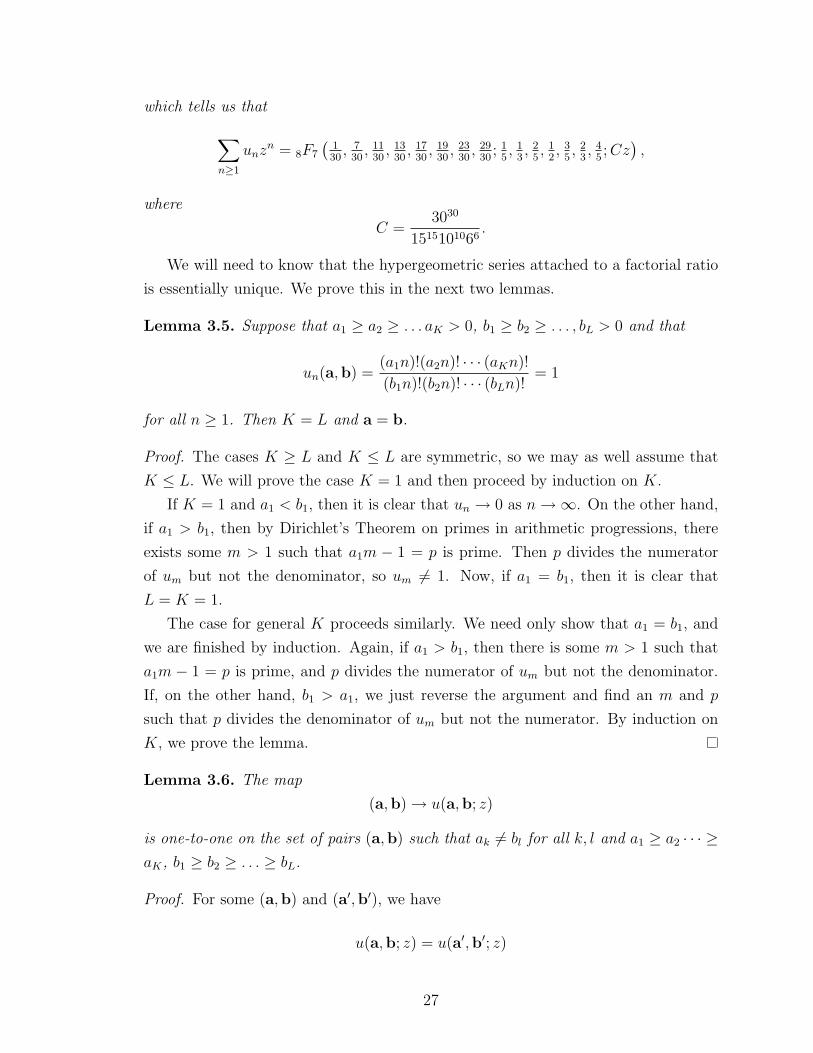
which tells us that∑n≥1
unzn = 8F7
(130, 7
30, 11
30, 13
30, 17
30, 19
30, 23
30, 29
30; 1
5, 1
3, 2
5, 1
2, 3
5, 2
3, 4
5;Cz
),
where
C =3030
1515101066.
We will need to know that the hypergeometric series attached to a factorial ratio
is essentially unique. We prove this in the next two lemmas.
Lemma 3.5. Suppose that a1 ≥ a2 ≥ . . . aK > 0, b1 ≥ b2 ≥ . . . , bL > 0 and that
un(a,b) =(a1n)!(a2n)! · · · (aKn)!
(b1n)!(b2n)! · · · (bLn)!= 1
for all n ≥ 1. Then K = L and a = b.
Proof. The cases K ≥ L and K ≤ L are symmetric, so we may as well assume that
K ≤ L. We will prove the case K = 1 and then proceed by induction on K.
If K = 1 and a1 < b1, then it is clear that un → 0 as n→∞. On the other hand,
if a1 > b1, then by Dirichlet’s Theorem on primes in arithmetic progressions, there
exists some m > 1 such that a1m − 1 = p is prime. Then p divides the numerator
of um but not the denominator, so um 6= 1. Now, if a1 = b1, then it is clear that
L = K = 1.
The case for general K proceeds similarly. We need only show that a1 = b1, and
we are finished by induction. Again, if a1 > b1, then there is some m > 1 such that
a1m − 1 = p is prime, and p divides the numerator of um but not the denominator.
If, on the other hand, b1 > a1, we just reverse the argument and find an m and p
such that p divides the denominator of um but not the numerator. By induction on
K, we prove the lemma.
Lemma 3.6. The map
(a,b)→ u(a,b; z)
is one-to-one on the set of pairs (a,b) such that ak 6= bl for all k, l and a1 ≥ a2 · · · ≥aK, b1 ≥ b2 ≥ . . . ≥ bL.
Proof. For some (a,b) and (a′,b′), we have
u(a,b; z) = u(a′,b′; z)
27

if and only if
un(a,b) = un(a′,b′)
for all n. In this case, we can rewrite this as
un(a,b)(un(a′,b′))−1 = un(a ∪ b′,b ∪ a′) = 1.
Now it follows from Lemma 3.5 that a ∪ b′ is a permutation of b ∪ a′. Thus a′ is a
permutation of a and b′ is a permutation of b.
Remark 3.7. It is also possible to state Lemma 3.6 in an algorithmic manner. Roughly
speaking, given parameters α = (α1, . . . , αd) and β = (β1, . . . , βd−1) that come from
a factorial ratio, we can form the polynomials P (x) and Q(x) from Definition 3.1. It
is then possible to add extra factors to P (x) and Q(x) together to obtain
P (x)
Q(x)=
(xa1 − 1)(xa2 − 1) · · · (xaK − 1)
(xb1 − 1)(xb2 − 1) · · · (xbL − 1)
and to recover a and b. In this manner, if we did not already know about the 52
sporadic integer factorial ratio sequences from Vasyunin’s work, we could recover
them from the work of Beukers and Heckman [6] described in Section 3.3.1.
The main interest in looking at hypergeometric series attached to factorial ratio
sequences comes from the following observation of Rodriguez-Villegas [25].
Theorem 3.8 (Rodriguez-Villegas [25]). Let
un(a,b) =(a1n)!(a2n)! · · · (aKn)!
(b1n)!(b2n)! · · · (bLn)!
with∑K
K=1 ak =∑L
l=1 bl and let
u(a,b; z) =∞∑n=0
un(a,b)zn.
Then u(a,b; z) is algebraic over Q(z) if and only if L − K = 1 and un(a,b) ∈Z for all n ≥ 0.
Proof of Theorem 3.8, part 1. We begin by proving that if the generating function is
algebraic, then un is in fact integral. In particular, it follows from Lemmas 2.2 and
2.4 that this will imply that we must have L −K ≥ 1, which is, in fact, all that we
need from this part of the proof.
28

A theorem of Eisenstein (see [18]) asserts that if u(a; b; z) is algebraic, then there
exists an N such that un(a,b) · Nn in an integer for all n. But Lemma 2.3 implies
that the set of primes occurring in the denominator of some un(a,b) is either empty
or infinite. So, if such an N exists, then we are able to take N = 1, which implies
that un(a,b) is an integer for all n.
The remainder of this proof relies on Landau’s theorem and the following lemma
of Beukers and Heckman [6].
Lemma 3.9 (Beukers–Heckman [6]). Let α1, α2, . . . αn and β1, β2, . . . βn−1 be rational
numbers with common denominator M . The hypergeometric function
nFn−1(α1, α2, . . . αn; β1, β2, . . . βn−1; z)
is algebraic if and only if for all k relatively prime to M the sequences
e(kα1), . . . , e(kαn)
and
e(kβ1), . . . , e(kβn−1), 1
interlace on the unit circle.
Proof. This follows from [6, Theorem 4.8] and the fact that this function is algebraic
if and only if its monodromy group is finite.
For the case of the hypergeometric functions that are generating series for un(a,b)
we can make this lemma slightly stronger.
Lemma 3.10. For a and b positive integer vectors, the function
u(a; b; z) =∞∑n=0
un(a,b)zn
is an algebraic function if and only if α = α(a,b) and β = β(a,b) interlace on [0, 1].
Proof. In our case the αi and βj are rational numbers in (0, 1]. Suppose that they
have common denominator M . Recall that the numbers e(αi) are roots of the
polynomial P (a,b;x), and that P is the product of cyclotomic polynomials, say
P = Φm1Φm2 · · ·Φml . Then for any (k,M) = 1 we also have (k,mi) = 1 for all mi.
So the map α→ αk simply permutes the roots of any Φmi . In particular, it permutes
the roots of P , and hence permutes the numbers e(αi).
29

The exact same argument applies for β. Thus we have that α and β interlace
on [0, 1] if and only if e(αi)k and e(βj)
k interlace on the unit circle for all k with
(k,M) = 1.
In particular, u(a; b; z) is algebraic if and only if α and β interlace on [0, 1].
Combining these lemmas finishes the proof of 3.8.
Proof of Theorem 3.8, part 2. Suppose that u(a,b; z) is algebraic. Then we know
that L −K ≥ 1, from the first part of the proof. Note that the number of copies of
the number 1 in the set β is L −K. However, if α and β are to interlace, no values
can be repeated, so we must have L−K = 1.
Now, if L − K = 1, then from Lemma 2.5 we know that un(a,b) is integral if
and only if α and β interlace. From Lemma 3.10 we know that this is equivalent to
u(a,b; z) being algebraic.
3.3 A Classification of Integral Factorial Ratios
3.3.1 Monodromy for Hypergeometric Functions nFn−1
This section is an application of the work of Beukers and Heckman [6], so we begin
by restating a few necessary theorems and definitions.
Definition 3.11 (Hypergeometric Groups). Let w1, . . . , wn and z1, . . . zn be complex
numbers with wi 6= zj for all i and j. The hypergeometric group H(w, z) with nu-
merator parameters w1, . . . , wn and denominator parameters z1, . . . , zn is a subgroup
of GLn(C) generated by elements
h0, h1, and, h∞
such that
h0h1h∞ = 1
and
det(t− h∞) =n∏j=1
(t− wj)
det(t− h−10 ) =
n∏j=1
(t− zj)
and such that h1 − 1 has rank 1.
30

Hypergeometric groups are precisely those groups which occur as monodromy
groups for hypergeometric functions. Specifically, we have the following.
Proposition 3.12. The monodromy group for the hypergeometric function
nFn−1(α1, . . . , αn; β1, . . . , βn−1; z),
with αiβj ∈ C, is a hypergeometric group with numerator parameters
e(α1), e(α2), . . . , e(αn)
and denominator parameters
e(β1), e(β2), . . . , e(βn−1), 1,
where e(z) = e2πiz.
Proof. This is [6, Proposition 3.2].
In categorizing hypergeometric groups it is useful to consider the following special
subgroup.
Definition 3.13. The subgroup Hr(w, z) of H(w, z) generated by hk∞h1h−k∞ for k ∈ Z
is called the reflection subgroup of H(w, z).
Also, the classification of hypergeometric groups splits into a primitive case and
an imprimitive case, as in the following definition.
Definition 3.14. Let G ⊂ GL(V ) be a subgroup acting irreducibly on a complex
vector space V . G is called imprimitive if there exists a direct sum decomposition
V = V1 ⊕ V2 ⊕ · · · ⊕ Vn with n > 1 and dimVi > 0 for all i such that the action of G
on V permutes the subspaces Vi. Otherwise, G is called primitive.
The existence of the following two theorems explains some of the usefulness of
considering the reflection subgroup of a hypergeometric group and in considering
when a hypergeometric group is primitive.
Theorem 3.15. The reflection subgroup Hr(w, z) of H(w, z) acts reducibly on Cn if
and only if there exists a root of unity ζ 6= 1 such that multiplication by ζ permutes
both the elements of w and the elements of z. Moreover, if Hr(w, z) is reducible, then
H(w, z) is imprimitive.
31

Proof. This is [6, Theorem 5.3].
Theorem 3.16. Suppose that Hr(w, z) is irreducible. Then H is imprimitive if and
only if there exist p, q ∈ N with p+ q = n and (p, q) = 1, and A,B,C ∈ C∗ such that
An = BpCq and such that
{w1, . . . , wn} = {A,Aζn, Aζ2n, . . . , Aζ
n−1n }
and
{z1, . . . , zn} = {B,Bζp, Bζ2p , . . . , Bζ
p−1p , C, Cζq, Cζ
2q , . . . , Cζ
q−1q }
where ζn = e(1/n), or with the same sets of equalities with w and z reversed.
Proof. This is [6, Theorem 5.8].
As defined, hypergeometric groups are subgroups of GLn(C). The following propo-
sition tells us when a hypergeometric group is defined over GLn(R) for R ⊂ C.
Proposition 3.17. Suppose w1, . . . , wn, z1, . . . , zn ∈ C∗ with wi 6= zj for all i, j. Let
A1, . . . An, B1, . . . , Bn be defined by
n∏j=1
(t− wj) = tn + A1tn−1 + · · ·+ An,
andn∏j=1
(t− zj) = tn +B1tn−1 + · · ·+Bn.
Then relative to a suitable basis, the hypergeometric group H(w, z) is defined over the
ring Z[A1, . . . , An, B1, . . . , Bn, A−1n , B−1
n ].
Proof. This is [6, Corollary 3.6], and follows directly from a theorem of Levelt [22,
Theorem 1.1].
We need to state one more definition, and then we will be ready to state the main
classification theorem of Beukers and Heckman that we are interested in.
Definition 3.18. A scalar shift of the hypergeometric group H(w, z) is a hypergeo-
metric group H(dw, dz) = H(dw1, dw2, . . . , dwn; dz1, dz2, . . . , dzn) for some d ∈ C∗.
Our main interest in the work of Beukers and Heckman comes from the following
Theorem.
32

Theorem 3.19. Let n ≥ 3 and let H(w, z) ⊂ GLn(C) be a primitive hyperge-
ometric group whose parameters are roots of unity and generate the field Q(ζh).
Then H(w, z) is finite if and only if, up to a scalar shift, the parameters have the
form wk1 , wk2 , . . . , w
kn; zk1 , z
k2 , . . . , z
kn, where gcd(h, k) = 1 and the exponents of either
w1, . . . , wn; z1, . . . , zn or z1, . . . , zn;w1, . . . wn are listed in [6, Table 8.3].
Proof. This is [6, Theorem 7.1].
3.3.2 The Classification
From now on we set L = K + 1. We are interested in ratios where the parameters
have greatest common divisor 1. The following lemma shows that this condition
translates nicely into the reflection group of the monodromy group being irreducible.
Lemma 3.20. Let un = un(a,b) and u = u(a,b; z). Let H(u) be the hypergeometric
group associated to u and let Hr(u) be the reflection subgroup of H(u). Suppose that
un is an integer for all n. Then Hr(u) acts reducibly on C if and only if
gcd(a1, a2, . . . , aK , b1, b2, . . . , bK+1) > 1.
Moreover, if Hr(u) is reducible, then H(u) is imprimitive.
Proof. Let P = P (a,b;x) and Q = Q(a,b;x). Then we have
P
Q=
(x− e(α1)) · · · (x− e(αd))(x− e(β1)) · · · (x− e(βd))
=(xa1 − 1) · · · (xaK − 1)
(xb1 − 1) · · · (xbK+1 − 1),
and H(u) is a hypergeometric group with numerator parameters
e(α1), e(α2), . . . , e(αd)
and denominator parameters
e(β1), e(β2), . . . , e(βd).
From Theorem 3.15 we know that Hr(u) acts reducibly on C if and only if there exists
some γ 6≡ 0 (mod 1) such that
{e(α1), e(α2), . . . , e(αd)} = {e(α1 + γ), e(α2 + γ), . . . , e(αd + γ)}
33

and
{e(β1), e(β2), . . . , e(βd)} = {e(β1 + γ), e(β2 + γ), . . . , e(βd + γ)}.
In this case, e(γ) is necessarily a primitive Mth root of unity for some M , and by
raising it to an appropriate power we may assume that γ is a primitive pth root of
unity for some prime p. We will show that if multiplication by e(γ) gives the desired
permutations, then p divides all of the ak and all of the bj.
Recall that P and Q are products of cyclotomic polynomials, and let ZM denote
the set of primitive M -th roots of unity. Notice that if (M, p) = 1, then multiplication
by e(γ) maps all primitive M -th roots of unity to primitive Mp-th roots of unity, while
some primitive Mp-th roots of unity are mapped to others, and some are mapped
to primitive p-th roots of unity. Thus, multiplication by e(γ) gives a permutation of
ZM ∪ ZMp. On the other hand, multiplication by e(γ) simply permutes each of the
sets ZMpe for e > 1.
Thus, if multiplication by e(γ) separately permutes the αi and the βj, then when-
ever P or Q has a factor ΦM with (M, p) = 1, it must also have a factor ΦMp. Suppose
then that there were some al or bk coprime to p, and assume M be the largest such.
Then (xM − 1) would have ΦM as a factor and any other term (xak − 1) or (xbj − 1)
which had ΦM as a factor would necessarily have ΦMp as a factor as well. Ultimately,
one of the polynomials P or Q would not have the terms ΦM and ΦpM properly
paired as factors. Thus, if p does not divide gcd(a1, a2, . . . , ak, b1, b2, . . . , bl), then
multiplication by a primitive pth root of unity does not separately permute α(a,b)
and β(a,b).
On the other hand, if p does divide gcd(a1, a2, . . . , ak, b1, b2, . . . , bl), then multipli-
cation by e(1/p) permutes the roots of each of the factors (xak − 1) and (xbl − 1), and
hence it separately permutes the roots of P and the roots of Q.
Vasyunin noticed that the step functions corresponding to
un =(2an)!(bn)!
(an)!(2bn)![(a− b)n]!with b < a (3.4)
and
un =(2an)!(2bn)!
(an)!(bn)![(a+ b)n]!(3.5)
are nonnegative. Thus for both of these families, un is an integer for all n. It turns
out that when a and b are not both odd these two infinite families give exactly those
with factorial ratios with gcd 1 for which the hypergeometric group is imprimitive.
34

On the other hand, when a and b are both odd, these come from scalar shifts of the
hypergeometric groups associated to binomial coefficients.
Lemma 3.21. Let un = un(a,b) and u = u(a,b; z). Let H(u) be the hypergeometric
group associated to u and let Hr(u) be the reflection subgroup of H(u). Suppose that
un is an integer for all n and that Hr(u) is irreducible; i.e. gcd(a1, . . . , aK , b1, . . . , bL =
1. Then H(u) is imprimitive if and only if un is of the form (3.4) or (3.5) with a
and b not both odd.
Proof. Again let P = P (a,b;x) and Q = Q(a,b;x). Suppose that un is the of form
(3.4). Then we have
P
Q=
(x2a − 1)(xb − 1)
(x2b − 1)(xa − 1)(xa−b − 1)=
(xa + 1)
(xb + 1)(xa−b − 1),
which is in lowest terms if a and b are not both odd. Then the numerator parameters
for H(u) are
A,Aζ1a , Aζ
2a , . . . , Aζ
a−1a
and the denominator parameters are
B,Bζb, Bζ2b , . . . , Bζ
b−1b , Cζa−b, Cζ
2a−b, . . . , Cζ
a−b−1a−b , 1
where A = ζ2a, B = ζ2b, and C = 1 satisfy Aa = BbCa−b = −1, so these parameters
satisfy the condition of Theorem 3.16, and H(u) is imprimitive.
Similarly, if un is of the form (3.5) then we have
P
Q=
(x2a − 1)(x2b − 1)
(xa − 1)(xb − 1)(xa+b − 1)=
(xa + 1)(xb + 1)
xa+b − 1,
again in lowest terms if a and b are not both odd, and so H(u) is a hypergeometric
group with numerator parameters
A,Aζ1a , Aζ
2a , . . . , Aζ
a−1a , B,Bζb, Bζ
2b , . . . , Bζ
b−1b
and denominator parameters
Cζa+b, Cζ2a+b, . . . , Cζ
a+ba+b
where A = ζ2a, B = ζ2b, and C = 1. A and B satisfy Aa = Bb = −1, so AaBb = 1 =
Ca+b, so H(u) again satisfies the conditions of the theorem.
35

To see the converse, suppose that the numerator parameters of H(u) are of the
form
A,Aζa, Aζ2a , . . . , Aζ
a−1a .
These parameters must have the property that, if they contain one primitive Mth
root of unity for some M , then they contain all of them. Thus, by symmetry con-
siderations, we find that the only possibilities are that A = 1 or A = ζ2a. However,
we cannot have A = 1, as one of the denominator parameters for a hypergeometric
group coming from an integral factorial ratio sequence will be 1, and the numerator
and denominator parameters must be distinct. Thus, A = ζ2a. Similarly, for the
denominator parameters we find that either B or C is 1, and so without loss of gen-
erality, we assume that C = 1 and find that B = ζ2b is the only possibility. Indeed,
whenever (a, b) = 1 and a and b are not both odd, this does work and gives un of the
form (3.4).
A similar argument works for the second case.
We now examine the case where both a and b are odd.
Lemma 3.22. Let un = un(a,b) and u = u(a,b; z). Let H(u) be the hypergeometric
group associated to u.
(i) If un is of the form (3.4) with a and b both odd, then H(u) is a scalar shift by
−1 = e(1/2) of H(u′), where
u′n =
(an
bn
).
(ii) If un is of the form (3.5) with a and b both odd, then H(u) is obtained by taking a
scalar shift of H(u′) and reversing the numerator and denominator parameters,
where
u′n =
((a+ b)n
an
).
Proof. (i) Suppose that un is of the form (3.4). Then, as in the previous lemma, we
have for P (x) = P (a,b;x) and Q(x) = Q(a,b;x),
P (x)
Q(x)=
(xa + 1)
(xb + 1)(xa−b − 1).
This is not in lowest terms, but it is in a convenient form for computing the scalar
shift of H(u). The scalar shift corresponds to multiplying each root of P and Q by
36

−1, in which case we obtain polynomials P ∗ and Q∗ with
P ∗(x)
Q∗(x)=
(xa − 1)
(xb − 1)(xa−b − 1),
which very clearly come from u′n =(anbn
).
(ii) If un is of the form (3.5), we proceed similarly, except that this time we find
thatP ∗(x)
Q∗(x)=
(xa − 1)(xb − 1)
(xa+b − 1),
which we can see comes from u′n =((a+b)nan
), with the numerator and denominator
parameters reversed.
We are now ready to prove Theorem 1.1
Proof of Theorem 1.1. Lemma 3.21 classifies all of those integral factorial ratios whose
associated hypergeometric group is imprimitive, so it remains to classify those with
gcd(a1, . . . , aK , b1, . . . , bL), whose associated hypergeometric groups are primitive.
Beukers and Heckman have categorized all finite primitive hypergeometric groups,
so we can examine [6, Table 8.3] to find all integral factorial ratios with associated
primitive hypergeometric groups.
Specifically, if H is a primitive hypergeometric group that comes from an integral
factorial ratio sequence, then H is either one of the entries in [6, Table 8.3] or a scalar
shift of one of the entries, possibly with the numerator and denominator parameters
reversed. Moreover, if H has numerator parameters α1, . . . , αd and denominator
parameters β1, . . . , βd, then the polynomials P (x) =∏
(x− e(αi)) and Q(x) =∏
(x−e(βj)) must have coefficients in Z. Aside from Line 1, there are 26 entries in the
table with this property. Moreover, Beukers and Heckman list the entries in the table
so that if the polynomials P and Q formed from the numerator and denominator
parameters of an entry have coefficients in a field K, then the polynomials formed
from a scalar shift of that entry will never have coefficients in a proper subfield of K,
so we only need to consider these 26 entries, along with Line 1, which we will mention
momentarily.
As the denominator parameters for a hypergeometric group coming from a fac-
torial ratio must contain a 1, there are only a finite number of scalar shifts of each
entry that we need to consider. It is easy to enter the data from [6, Table 8.3] into a
computer program and to check each of the scalar shifts of each of these 26 entries. It
turns out that there are 52 hypergeometric group parameter sets coming from integral
37

factorial ratios, and these are all given by these 26 entries and scalar shifts by −1 of
these entries, possibly with numerator and denominator parameters reversed.
It is easily seen that Line 1 of [6, Table 8.3] corresponds to the infinite family of
binomial coefficient sequences
[(a+ b)n]!
(an)!(bn)!with gcd(a, b) = 1,
and, as we have seen in Lemma 3.22, scalar shifts of this family by −1 yield factorial
ratios of the forms (3.4) and (3.5) already considered. We need only to rule out other
scalar shifts for this family.
The scalar shifts of this family that we need to consider are shifts by roots of unity
of the form e(−n/a), e(−n/b) and e( −na+b
). The cases of multiplication by e(−n/a)
and e(−n/b) are symmetric, so let us consider multiplication by ζ = e(−n/a). ζ is a
primitive Mth root of unity for some M dividing a, so we may as well assume that
ζ = e(1/M). But then ζ · e(1/b) is a primitive bM -th root of unity, as (M, b) = 1. If
M 6= 2 then some of the primitive bM -th roots of unity are mapped to themselves by
multiplication by e(1/M), so not all primitive bM -th roots of unity can be obtained
in this way, so the polynomials P and Q obtained from this shift cannot have integer
coefficients unless M = 2, which is the case of a scalar shift by −1.
The case for multiplication by a root of the form e( −na+b
)is completely similar,
since a, b, and a+ b are relatively prime in pairs.
Lemma 3.6 assures us that this must be all integer factorial ratio sequences in
which the parameters have greatest common divisor 1, giving us the “only if” part of
the theorem.
3.4 A Listing of all Integral Factorial Ratios with L−K = 1
The following tables contain a listing of all integer factorial ratios with gcd 1, orga-
nized as follows. The second column lists the parameters for un(a,b). The parameter
d of the third column is the dimension of the monodromy group of u(a,b; z), and the
fourth column lists the specific parameters for dFd−1. With the exception of lines 2
and 3 of Table 3.1 all the entries have primitive monodromy groups, and so they have
a corresponding entry in [6, Table 8.3].
It should be noted that lines 1, 2, and 3 of Table 3.1 only correspond to solutions
with gcd 1 when gcd(a, b) = 1.
38

Table 3.1: The three infinite families of integral factorialratio sequences
Line # un(a,b) d dFd−1 parameters [6] Line #
1a,b[a+b]
[a,b]a+ b− 1
[ 1a+b
, 2a+b
,...,a+b−1a+b
]
[ 1a, 2a,...,a−1
a, 1b, 2b,..., b−1
b]
1
2a,b[2a,b]
[a,2b,a−b]a
[ 12a, 32a,... 2a−1
2a]
[ 12b, 32b,... 2b−1
2b, 1a−b ,
2a−b ,...,
a−b−1a−b ]
None
3a,b[2a,2b]
[a,b,a+b]a+ b
[ 12a, 32a,... 2a−1
2a, 12b, 32b,... 2b−1
2b]
[ 1a+b
, 2a+b
,...,a+b−1a+b
]None
Table 3.2: The 52 sporadic integral factorial ratio se-quences
Line # un(a,b) d dFd−1 parameters [6] Line #
1[12,1]
[6,4,3]4
[ 112, 512, 712, 1112 ]
[ 13, 12, 23 ]
37
2[12,3,2]
[6,6,4,1]4
[ 112, 512, 712, 1112 ]
[ 16, 12, 56 ]
37
3[12,1]
[8,3,2]6
[ 112, 16, 512, 712, 56, 1112 ]
[ 18, 38, 12, 58, 78 ]
45
4[12,3]
[8,6,1]6
[ 112, 13, 512, 712, 23, 1112 ]
[ 18, 38, 12, 58, 78 ]
45
5[12,3]
[6,5,4]6
[ 112, 13, 512, 712, 23, 1112 ]
[ 15, 25, 12, 35, 45 ]
46
6[12,5]
[10,4,3]6
[ 112, 16, 512, 712, 56, 1112 ]
[ 110, 310, 12, 710, 910 ]
46
7[18,1]
[9,6,4]6
[ 118, 518, 718, 1118, 1318, 1718 ]
[ 14, 13, 12, 23, 34 ]
47
8[9,2]
[6,4,1]6
[ 19, 29, 49, 59, 79, 89 ]
[ 16, 14, 12, 34, 56 ]
47
9[9,4]
[8,3,2]6
[ 19, 29, 49, 59, 79, 89 ]
[ 18, 38, 12, 58, 78 ]
48
10[18,4,3]
[9,8,6,2]6
[ 118, 518, 718, 1118, 1318, 1718 ]
[ 18, 38, 12, 58, 78 ]
48
11[9,1]
[5,3,2]6
[ 19, 29, 49, 59, 79, 89 ]
[ 15, 25, 12, 35, 45 ]
49
12[18,5,3]
[10,9,6,1]6
[ 118, 518, 718, 1118, 1318, 1718 ]
[ 110, 310, 12, 710, 910 ]
49
39

Line # un(a,b) d dFd−1 parameters [6] Line #
13[18,4]
[12,9,1]7
[ 118, 518, 718, 12, 1118, 1318, 1718 ]
[ 112, 13, 512, 712, 23, 1112 ]
58
14[12,2]
[9,4,1]7
[ 112, 16, 512, 12, 712, 56, 1112 ]
[ 19, 29, 49, 59, 79, 89 ]
58
15[18,2]
[9,6,5]7
[ 118, 518, 718, 12, 1118, 1318, 1718 ]
[ 15, 13, 25, 35, 23, 45 ]
59
16[10,6]
[9,5,2]7
[ 110, 16, 310, 12, 710, 56, 910 ]
[ 19, 29, 49, 59, 79, 89 ]
59
17[14,3]
[9,7,1]7
[ 114, 314, 514, 12, 914, 1114, 1314 ]
[ 19, 29, 49, 59, 79, 89 ]
60
18[18,3,2]
[9,7,6,1]7
[ 118, 518, 718, 12, 1118, 1318, 1718 ]
[ 17, 27, 37, 47, 57, 67 ]
60
19[12,2]
[7,4,3]7
[ 112, 16, 512, 12, 712, 56, 1112 ]
[ 17, 27, 37, 47, 57, 67 ]
61
20[14,6,4]
[12,7,3,2]7
[ 114, 314, 514, 12, 914, 1114, 1314 ]
[ 112, 13, 512, 712, 23, 1112 ]
61
21[14,1]
[7,5,3]7
[ 114, 314, 514, 12, 914, 1114, 1314 ]
[ 15, 13, 25, 35, 23, 45 ]
62
22[10,6,1]
[7,5,3,2]7
[ 110, 16, 310, 12, 710, 56, 910 ]
[ 17, 27, 37, 47, 57, 67 ]
62
23[15,1]
[9,5,2]8
[ 115, 215, 415, 715, 815, 1115, 1315, 1415 ]
[ 19, 29, 49, 12, 59, 79, 89 ]
63
24[30,9,5]
[18,15,10,1]8
[ 130, 730, 1130, 1330, 1730, 1930, 2330, 2930 ]
[ 118, 518, 718, 12, 1118, 1318, 1718 ]
63
25[15,4]
[12,5,2]8
[ 115, 215, 415, 715, 815, 1115, 1315, 1415 ]
[ 112, 16, 512, 12, 712, 56, 1112 ]
64
26[30,5,4]
[15,12,10,2]8
[ 130, 730, 1130, 1330, 1730, 1930, 2330, 2930 ]
[ 112, 13, 512, 12, 712, 23, 1112 ]
64
27[15,4]
[8,6,5]8
[ 115, 215, 415, 715, 815, 1115, 1315, 1415 ]
[ 18, 16, 38, 12, 58, 56, 78 ]
65
28[30,5,4]
[15,10,8,6]8
[ 130, 730, 1130, 1330, 1730, 1930, 2330, 2930 ]
[ 18, 13, 38, 12, 58, 23, 78 ]
65
29[15,2]
[10,4,3]8
[ 115, 215, 415, 715, 815, 1115, 1315, 1415 ]
[ 110, 14, 310, 12, 710, 34, 910 ]
66
30[30,3,2]
[15,10,6,4]8
[ 130, 730, 1130, 1330, 1730, 1930, 2330, 2930 ]
[ 15, 14, 25, 12, 35, 34, 45 ]
66
31[30,1]
[15,10,6]8
[ 130, 730, 1130, 1330, 1730, 1930, 2330, 2930 ]
[ 15, 13, 25, 12, 35, 23, 45 ]
67
40

Line # un(a,b) d dFd−1 parameters [6] Line #
32[15,2]
[10,6,1]8
[ 115, 215, 415, 715, 815, 1115, 1315, 1415 ]
[ 110, 16, 310, 12, 710, 56, 910 ]
67
33[15,7]
[14,5,3]8
[ 115, 215, 415, 715, 815, 1115, 1315, 1415 ]
[ 114, 314, 514, 12, 914, 1114, 1314 ]
68
34[30,5,3]
[15,10,7,6]8
[ 130, 730, 1130, 1330, 1730, 1930, 2330, 2930 ]
[ 17, 27, 37, 12, 47, 57, 67 ]
68
35[30,5,3]
[15,12,10,1]8
[ 130, 730, 1130, 1330, 1730, 1930, 2330, 2930 ]
[ 112, 14, 512, 12, 712, 34, 1112 ]
69
36[15,6,1]
[12,5,3,2]8
[ 115, 215, 415, 715, 815, 1115, 1315, 1415 ]
[ 112, 14, 512, 12, 712, 34, 1112 ]
69
37[15,1]
[8,5,3]8
[ 115, 215, 415, 715, 815, 1115, 1315, 1415 ]
[ 18, 14, 38, 12, 58, 34, 78 ]
70
38[30,5,3,2]
[15,10,8,6,1]8
[ 130, 730, 1130, 1330, 1730, 1930, 2330, 2930 ]
[ 18, 14, 38, 12, 58, 34, 78 ]
70
39[20,3]
[12,10,1]8
[ 120, 320, 720, 920, 1120, 1320, 1720, 1920 ]
[ 112, 16, 512, 12, 712, 56, 1112 ]
71
40[20,6,1]
[12,10,3,2]8
[ 120, 320, 720, 920, 1120, 1320, 1720, 1920 ]
[ 112, 13, 512, 12, 712, 23, 1112 ]
71
41[20,1]
[10,8,3]8
[ 120, 320, 720, 920, 1120, 1320, 1720, 1920 ]
[ 18, 13, 38, 12, 58, 23, 78 ]
72
42[20,3,2]
[10,8,6,1]8
[ 120, 320, 720, 920, 1120, 1320, 1720, 1920 ]
[ 18, 16, 38, 12, 58, 56, 78 ]
72
43[20,1]
[10,7,4]8
[ 120, 320, 720, 920, 1120, 1320, 1720, 1920 ]
[ 17, 27, 37, 12, 47, 57, 67 ]
73
44[20,7,2]
[14,10,4,1]8
[ 120, 320, 720, 920, 1120, 1320, 1720, 1920 ]
[ 114, 314, 514, 12, 914, 1114, 1314 ]
73
45[20,3]
[10,9,4]8
[ 120, 320, 720, 920, 1120, 1320, 1720, 1920 ]
[ 19, 29, 49, 12, 59, 79, 89 ]
74
46[20,9,6]
[18,10,4,3]8
[ 120, 320, 720, 920, 1120, 1320, 1720, 1920 ]
[ 118, 518, 718, 12, 1118, 1318, 1718 ]
74
47[24,1]
[12,8,5]8
[ 124, 524, 724, 1124, 1324, 1724, 1924, 2324 ]
[ 15, 14, 25, 12, 35, 34, 45 ]
75
48[24,5,2]
[12,10,8,1]8
[ 124, 524, 724, 1124, 1324, 1724, 1924, 2324 ]
[ 110, 14, 310, 12, 710, 34, 910 ]
75
49[24,4,1]
[12,8,7,2]8
[ 124, 524, 724, 1124, 1324, 1724, 1924, 2324 ]
[ 17, 27, 37, 12, 47, 57, 67 ]
76
50[24,7,4]
[14,12,8,1]8
[ 124, 524, 724, 1124, 1324, 1724, 1924, 2324 ]
[ 114, 314, 514, 12, 914, 1114, 1314 ]
76
41

Line # un(a,b) d dFd−1 parameters [6] Line #
51[24,4,3]
[12,9,8,2]8
[ 124, 524, 724, 1124, 1324, 1724, 1924, 2324 ]
[ 19, 29, 49, 12, 59, 79, 89 ]
77
52[24,9,6,4]
[18,12,8,3,2]8
[ 124, 524, 724, 1124, 1324, 1724, 1924, 2324 ]
[ 118, 518, 718, 12, 1118, 1318, 1718 ]
77
42

CHAPTER 4
Proof of Theorem 1.2
4.1 Introduction
In this chapter, which is joint work with Jason Bell [5], we give a proof of Theorem
1.2*, which we recall gives a relation between the height and the length of a balanced
nonnegative step function of the form
f(x; a,b) =K∑k=1
bakxc −L∑l=1
bblxc .
From Lemma 2.5, this also proves Theorem 1.2. We recall that the theorem we wish
to prove is
Theorem 1.2*. Fix L−K = D. If
f(x) =K∑k=1
bakxc −L∑l=1
bblxc
whereK∑k=1
ak =L∑l=1
bl
and ak 6= bl, ak, bl ∈ {1, 2, 3, . . .} for all k, l, and if
f(x) ≥ 0
for all x, then
K + L� D2(logD)2.
From Lemma 2.4 we know that if∑ak =
∑bl, then f(x; a,b) is nonnegative if
and only if its maximum value is exactly L − K. Therefore in order to prove that
43

such a function cannot be nonnegative if L+K is large (in terms of L−K) we will
show that f(x) must take on large values if L+K is large. We do this by giving the
following explicit lower bound on the L2 norm of f .
Theorem 4.1. Let
f(x) =K∑k=1
bakxc −L∑l=1
bblxc
whereK∑k=1
ak =L∑l=1
bl
and ak 6= bl, ak, bl ∈ {1, 2, 3, . . .} for all k, l. Then for all M > 285
∫ 1
0
f(x)2dx ≥ (K − L)2
4+
(K + L)
2π2
[e−γ
(logM)
(1− 1
2(logM)2
)]2
− (K + L)2
2π2
[2
(M − 1)1/2
(e−γ
(logM)
(1− 1
2(logM)2
))−1
+1
M − 1
], (4.1)
where γ := limN→∞
(∑Nn=1
1n− log n
)≈ 0.577215664901533 is Euler’s constant.
Remark 4.2. In this theorem M is a parameter that we will be free to choose to
optimize this lower bound. We obtain easily stated asymptotic results below by
choosing M = (K+L)4 and give examples of optimized bounds that can be obtained
in Section 4.3. (The condition that M > 285 in the above statement comes from
our use of Rosser and Schoenfeld’s [26] explicit formulation of Merten’s Theorem (see
Lemma 4.8).)
Granting this theorem for a moment, we may now easily prove Theorem 1.2*.
Proof of Theorem 1.2*. Take M to be (K+L)4. Then for fixed K−L, equation (4.1)
gives
maxx∈R|f(x)|2 ≥
∫ 1
0
f(x)2dx� (K + L)
(log(K + L))2.
Now let N = K + L and A = maxx∈R |f(x)|. Then we have
N
(logN)2� A2.
Additionally, since this implies that A� N1/3, we may write
N � N(logA)2
(logN)2� A2(logA)2. (4.2)
44

Now take D = L − K fixed. Lemma 2.4 says that if f(x) ≥ 0 for all x, then the
maximum value of f(x) is D. Thus A = D in this case, and Equation (4.2) gives the
desired bound.
4.1.1 Notation
bxc denotes the floor of x, which is the largest integer less than or equal to x.
{x} := x −bxc is the fractional part of x. Also e(x) := exp(2πix) := e2πix, and γ
denotes Euler’s constant
γ := limN→∞
(N∑n=1
1
n− log n
)≈ 0.577215664901533.
4.2 An explicit lower bound for the L2 norm
To prove Theorem 4.1, we will use Parseval’s identity, so we start by computing the
Fourier coefficients of f(x; a,b). Note that if f is balanced, so that∑ak =
∑bk, then
using the relation x =bxc+{x} we can rewrite f(x; a,b) as f(x; a,b) =∑L
l=1{blx}−∑Kk=1{akx}.
Lemma 4.3. Suppose that f(x) =∑L
l=1{blx} −∑K
k=1{akx}. Then the Fourier ex-
pansion of f is
f(x) =L−K
2+
1
2πi
∑n∈Zn 6=0
1
n
∑ak|n
ak −∑bl|n
bl
e(nx).
That is, f(0) = (L−K)/2 and for n 6= 0
f(n) =1
2πin
∑ak|n
ak −∑bl|n
bl
.Proof. The Fourier expansion for the fractional part of x is
{x} =1
2− 1
2πi
∑n∈Zn6=0
e(nx)
n. (4.3)
45
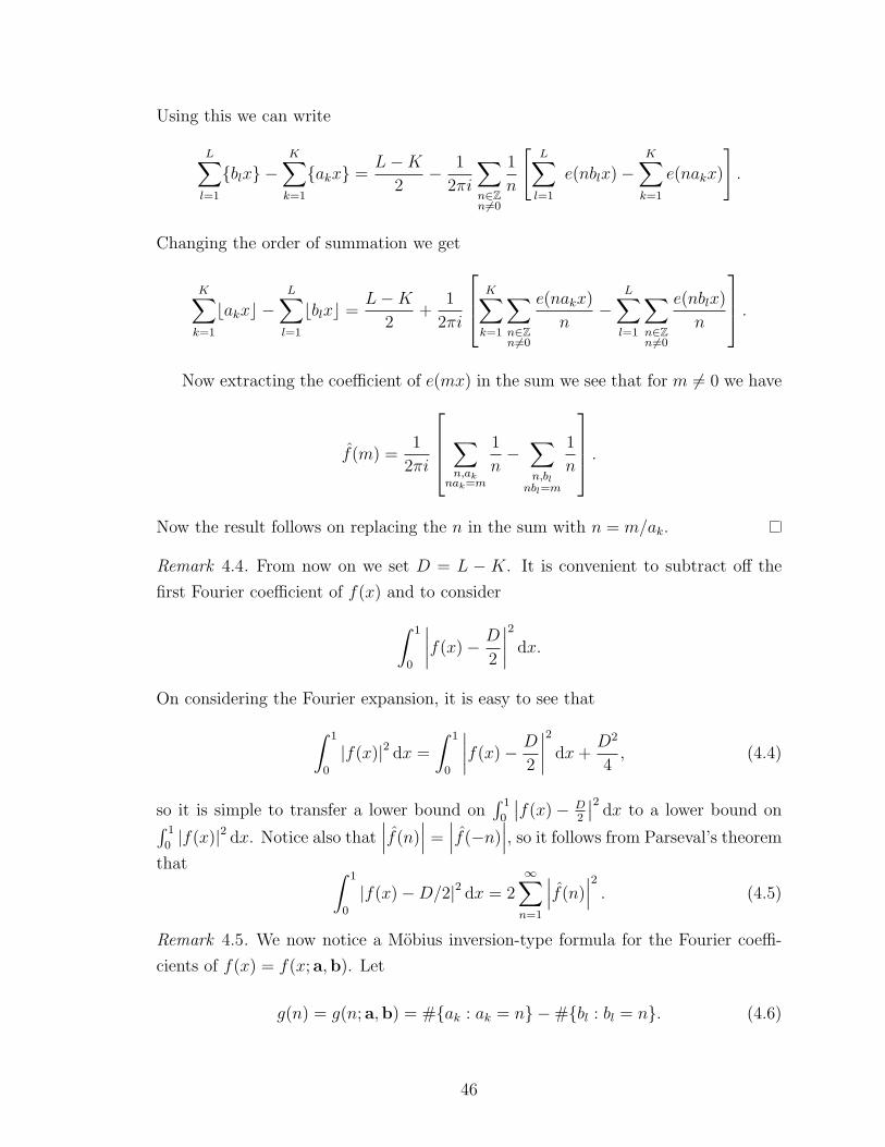
Using this we can write
L∑l=1
{blx} −K∑k=1
{akx} =L−K
2− 1
2πi
∑n∈Zn6=0
1
n
[L∑l=1
e(nblx)−K∑k=1
e(nakx)
].
Changing the order of summation we get
K∑k=1
bakxc −L∑l=1
bblxc =L−K
2+
1
2πi
K∑k=1
∑n∈Zn6=0
e(nakx)
n−
L∑l=1
∑n∈Zn6=0
e(nblx)
n
.Now extracting the coefficient of e(mx) in the sum we see that for m 6= 0 we have
f(m) =1
2πi
∑n,ak
nak=m
1
n−∑n,bl
nbl=m
1
n
.Now the result follows on replacing the n in the sum with n = m/ak.
Remark 4.4. From now on we set D = L − K. It is convenient to subtract off the
first Fourier coefficient of f(x) and to consider∫ 1
0
∣∣∣∣f(x)− D
2
∣∣∣∣2 dx.
On considering the Fourier expansion, it is easy to see that∫ 1
0
|f(x)|2 dx =
∫ 1
0
∣∣∣∣f(x)− D
2
∣∣∣∣2 dx+D2
4, (4.4)
so it is simple to transfer a lower bound on∫ 1
0
∣∣f(x)− D2
∣∣2 dx to a lower bound on∫ 1
0|f(x)|2 dx. Notice also that
∣∣∣f(n)∣∣∣ =
∣∣∣f(−n)∣∣∣, so it follows from Parseval’s theorem
that ∫ 1
0
|f(x)−D/2|2 dx = 2∞∑n=1
∣∣∣f(n)∣∣∣2 . (4.5)
Remark 4.5. We now notice a Mobius inversion-type formula for the Fourier coeffi-
cients of f(x) = f(x; a,b). Let
g(n) = g(n; a,b) = #{ak : ak = n} −#{bl : bl = n}. (4.6)
46

Then from Lemma 4.3 we see that for n ≥ 1 we have
f(n) =1
2πi
∑d|n
dg(d)
n.
Or, forming the Dirichlet series
G(s) = D(g, s) =∞∑n=1
g(n)
ns
(note that G is actually given by a finite sum) and
F (s) = D(f , s) =∞∑n=1
f(n)
ns,
we have the relation
G(s)ζ(s+ 1) = 2πiF (s), (4.7)
where ζ(s) = D(1, s) =∑∞
n=1 n−s is the Riemann ζ-function.
To estimate the mean square of f we use the following theorem of Carlson [14] to
relate∑∞
n=1
∣∣∣f(n)∣∣∣2 to a mean value of |G(it)|2.
Proposition 4.6. Let f(s) =∑∞
n=1 ann−s in some half-plane. Then if f(s) analyti-
cally continues to the half plane σ ≥ α and satisfies |f(σ + it)| � |t|A on all vertical
lines σ ≥ α, and if1
2T
∫ T
−T|f(α + it)|2 dt
is bounded as T →∞, then
limT→∞
1
2T
∫ T
−T|f(σ + it)|2 dt =
∞∑n=1
|an|2
n2σ.
Proof. See [30, Section 9.51].
It follows immediately from this proposition and the relation (4.7) that for all
σ > 0 we have
∞∑n=1
∣∣∣f(n)∣∣∣
n2σ= lim
T→∞
∫ T
−T|G(σ + it)ζ(1 + σ + it)|2 dt. (4.8)
Eventually we will let σ tend to zero, but first we estimate the right hand side of
47

(4.8) using a truncated Euler product for the ζ-function. Define the main term
ζM(s) =∏p≤M
(1− 1
ps
)−1
,
and let ζR(s) be defined by ζ(s) = ζM(s) + ζR(s). We will use the following lemmas
which give bounds on the size of ζM .
Lemma 4.7. If Re(s) ≥ 1 then
1
ζM(1)≤ |ζM(s)| ≤ ζM(1). (4.9)
Proof. This is just a restatement of the fact that for all s with real part greater than
1, and all integers n > 0, we have(1− 1
n
)≤∣∣∣∣1− 1
ns
∣∣∣∣−1
≤(
1− 1
n
)−1
.
Lemma 4.8 (Effective Mertens’ bound). For all M > 285,
ζM(1) ≤ logM
e−γ
(1− 1
2(logM)2
)−1
(4.10)
Proof. See Rosser and Schoenfeld [26, Theorem 7].
Proof of Theorem 4.1. We now write
1
2T
∫ T
−T|G(σ + it)ζ(1 + σ + it)|2 dt
=1
2T
∫ T
−T|G(σ + it)ζM(1 + σ + it)|2 dt+ E(M,T ),
where
E(M,T ) =1
2T
∫ T
−T|G(σ + it)| |ζM(1 + σ + it) + ζR(1 + σ + it)|2 dt
− 1
2T
∫ T
−T|G(σ + it)ζM(1 + σ + it)|2 dt.
Applying the triangle inequality in the form ||A| − |B|| ≤ |A−B| to the above, we
48
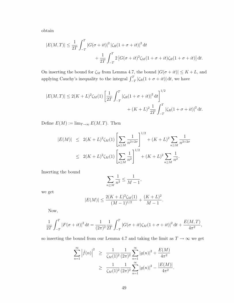
obtain
|E(M,T )| ≤ 1
2T
∫ T
−T|G(σ + it)|2 |ζR(1 + σ + it)|2 dt
+1
2T
∫ T
−T2∣∣G(σ + it)2ζM(1 + σ + it)ζR(1 + σ + it)
∣∣ dt.On inserting the bound for ζM from Lemma 4.7, the bound |G(σ + it)| ≤ K +L, and
applying Cauchy’s inequality to the integral∫ T−T |ζR(1 + σ + it)| dt, we have
|E(M,T )| ≤ 2(K + L)2ζM(1)
[1
2T
∫ T
−T|ζR(1 + σ + it)|2 dt
]1/2
+ (K + L)2 1
2T
∫ T
−T|ζR(1 + σ + it)|2 dt.
Define E(M) := limT→∞E(M,T ). Then
|E(M)| ≤ 2(K + L)2ζM(1)
[∑n≥M
1
n2+2σ
]1/2
+ (K + L)2∑n≥M
1
n2+2σ
≤ 2(K + L)2ζM(1)
[∑n≥M
1
n2
]1/2
+ (K + L)2∑n≥M
1
n2.
Inserting the bound ∑n≥M
1
n2≤ 1
M − 1,
we get
|E(M)| ≤ 2(K + L)2ζM(1)
(M − 1)1/2+
(K + L)2
M − 1.
Now,
1
2T
∫ T
−T|F (σ + it)|2 dt =
1
(2π)2
1
2T
∫ T
−T|G(σ + it)ζM(1 + σ + it)|2 dt+
E(M,T )
4π2,
so inserting the bound from our Lemma 4.7 and taking the limit as T →∞ we get
∞∑n=1
∣∣∣f(n)∣∣∣2 ≥ 1
ζM(1)2
1
(2π)2
∞∑n=1
|g(n)|2 +E(M)
4π2
≥ 1
ζM(1)2
1
(2π)2
∞∑n=1
|g(n)|2 − |E(M)|4π2
.
49

Putting in the bounds for E(M), we get
∞∑n=1
∣∣∣f(n)∣∣∣2 ≥ 1
ζM(1)2
1
(2π)2(K + L)− (K + L)2
4π2
[2ζM(1)
(M − 1)1/2+
1
M − 1
].
And finally, putting in the bounds on ζM(1), we get
∞∑n=1
∣∣∣f(n)∣∣∣2 ≥ (K + L)
4π2
[e−γ
(logM)
(1− 1
2(logM)2
)]2
− (K + L)2
4π2
[2
(M − 1)1/2
(e−γ
(logM)
(1− 1
2(logM)2
))−1
+1
M − 1
]. (4.11)
The theorem now follows immediately from (4.11) and fact that∫ 1
0
f(x)2dx = 2∞∑n=1
∣∣∣f(n)∣∣∣2 +
(K − L)2
4.
4.3 Explicit bounds and remarks
Let B(D) denote the maximal number of terms that a step function of the form
f(x; a,b) =K∑k=1
bakxc −L∑l=1
bblxc
may have if D = L − K, ai, bj ∈ N,∑ai =
∑bj and ai 6= bj for all i, j, and
f(x) ≥ 0 for all x. With this notation, Theorem 1.2* says that B(D) is finite, and
that, moreover B(D)� D2 logD. Using equation 4.11 we may compute some explicit
upper bounds on B(D).
For example, when D = 1 such a function f(x) that only takes on the values 0 and
1 must have∑∞
n=1
∣∣∣f(n)∣∣∣2 = 1
4. If K + L = 112371 and M = 1123714.96215, the right
side of 4.11 is ≈ 0.250000802. Additionally, the right side of (4.11) is an increasing
function of K + L when M is set to be a fixed power of K + L, so it follows that
B(1) < 112371.
Similarly we obtain B(2) < 502827 by taking L + K = 502827 and M =
5028274.6602, in which case the right side of (4.11) is ≈ 1.00000138, but it must be
the case that∑∞
n=1
∣∣∣f(b)∣∣∣2 ≤ 1 if f(x) takes values in precisely in the range {0, 1, 2}.
50

These bounds are far from best possible. From Theorem 1.1* we know that
B(1) = 9, and computations suggest that it might be the case that B(2) = 18.
Additionally, for the case of D = 3, a direct computer search has checked that there
are no functions with 29 terms that take values only in the range {0, 1, 2, 3} when∑ai =
∑bj ≤ 60. (However, the search space would have to be greatly enlarged for
this to be truly convincing evidence that B(3) = 27.)
51

CHAPTER 5
Proof of Theorem 1.3
In this section we prove a generalization of Theorem 1.1* which says that for any
fixed D = L−K, there exists a classification of nonnegative step functions
f(x; a,b) =K∑k=1
bakxc −L∑l=1
bblxc
such that∑ak =
∑bl similar to the classification given for D = 1. Specifically, if
we fix L and K, then the function f(x; a,b) is nonnegative for all x if and only if a
and b lie in a subset of RK+L which can be written as the union of a finite number
of subspaces of RK+L.
The theorem we will prove is
Theorem 1.3*. Fix positive integers K and L, and an integer A ≤ 0. The set S of
a1, a2, . . . , aK , b1, b2, . . . bL such that
1.∑ak =
∑bl
2. ak and bl are nonnegative integers for all k, l
3. A ≤∑K
k=1bakxc −∑L
l=1bblxc ≤ L−K − A
can be written as
S = (Z≥0)K+L
⋂(N⋃n=1
Vn
),
where each Vn is a subspace of RK+L.
We will prove this theorem as an application of a theorem of J. Lawrence [21]
about closed subgroups of the torus. Lawrence’s theorem is a theorem about the set
of subgroups which miss a given full subset of either Rn or Tn. We will not need the
52

full strength of Lawrence’s result here, though, because open subsets of the torus are
a particular example of full subsets. The result that we will use is
Theorem 5.1 ([21, Corollary 1.A]). If U is an open subset of Tn, then there are only
finitely many maximal open subgroups H of Tn such that H ∩ U = ∅.
Proof of Theorem 1.3*. Let F (x1, . . . xK , y1, . . . , yL) = −∑K
k=1{xk}+∑L
l=1{yl}, and
let V denote the subspace of RK+L defined by the equation∑K
k=1 xk =∑L
l=1 yl. We
may consider F as a function from RK+L to R, since F has period 1 in each of its
variables, we may consider it as a function from TK+L = RK+L/ZK+L to R. Note that,
when restricted to the subspace V , F (x1, . . . xK , y1, . . . , yL) =∑K
k=1bxkc −∑L
l=1bylc.For each subspace G of V let SG denote the set
SG := {(x1, . . . , xK , y1, . . . , yL) ∈ G such that F (x1, . . . , xK , y1, . . . yL) < A}.
Note that as F is not continuous, SG is not, in general, open. We will consider in
general, however whether or not SG contains an open set. In fact, we will show that
the set of subspaces G of V such that SG does not contain a nonempty open subset
(with respect to the subspace topology induced on G) has finitely many maximal
elements.
Granting this for a moment, let V1, V2, . . . , VN denote these subspaces. The condi-
tions that f(x; a,b) ≥ A for all x and f(x; a,b) ≤ L−K−A for all x are equivalent,
so we focus on the first. Suppose now that f(x; a,b) ≥ A for all x, and for some a,b
satisfying the desired properties. Then F (a1x, a2x, . . . , aKx, b1x, . . . , bLx) ≥ A for all
x, so we have a one dimensional subspace of RK+L on which F is larger than A, which
must be contained within one of the Vn. In particular, (a1, a2, . . . , aK , b1, . . . , bL) is
contained in one of the Vn.
On the other hand, suppose that some set of positive integers
(a1, a2, . . . , aK , b1, b2, . . . , bL) ∈ Vn, for some n.
We must show that f(x) = f(x; a,b) ≥ A for all x. We argue by contradiction,
constructing an open set in Vn where F (x1, . . . , xK , y1, . . . , yL) < A. Suppose that
f(c) < A. As all a1, . . . , aK , b1, . . . , bL are positive, f(x) is right continuous and
piecewise constant, so we may assume that f(x) < A for all x ∈ [c, d). Furthermore,
we may choose d small enough so that none of akx or blx is an integer for x ∈(c, d). Let x0 = (c + d)/2. Then F (x1, . . . , xK , y1, . . . , yL) is continuous at P =
(a1x0, a2x0, . . . , aKx0, b1x0, . . . , bLx0), and it is strictly less than A at this point. Thus
53

it is strictly less than A in an open neighborhood U of P . In particular, F < A
in U ∩ Vn, which is open with respect to the subspace topology on Vn, which is a
contradiction.
We now construct these maximal subgroups inductively using Lawrence’s theorem.
If SV does not contain a nonempty open subset, then we are done.
Otherwise, consider V ⊂ TK+L = RK+L/ZK+L, the image of V in the quotient.
Since V has a basis of rational vectors, V is a proper closed subgroup of TK+L. F is
periodic modulo 1 in each of its variables, so it is well defined on TK+L, so we may
consider SV as a subset of V . By assumption, it contains a nonempty open subset U .
V itself is a K + L − 1 dimensional torus, so by Theorem 5.1 the set of closed
subgroups G of V which miss U has finitely many maximal elements G1, . . . , Gm.
Each of these is a subgroup of dimension strictly less than the dimension of V , and,
in turn, for each of these subgroups SG either does or does not contain a nonempty
open set. If SG does not contain an open set, it is one of the maximal subgroups that
we are looking for. Otherwise, we proceed recursively, applying this same argument to
each G such that SG contains an open set, and ignoring discrete subgroups, Since the
dimension is reduced at each step, this process eventually terminates. Non-discrete
subgroups of TK+L are in one to one correspondence with subspaces of RK+L, so by
lifting these subgroups to RK+L we obtain the subgroups we are looking for.
54

BIBLIOGRAPHY
[1] Y. Andre. G-functions and geometry. Aspects of Mathematics, E13. Friedr.Vieweg & Sohn, Braunschweig, 1989.
[2] L. Baez-Duarte. New versions of the Nyman-Beurling criterion for the Riemannhypothesis. Int. J. Math. Math. Sci., 31(7):387–406, 2002.
[3] L. Baez-Duarte. A strengthening of the Nyman-Beurling criterion for the Rie-mann hypothesis. Atti Accad. Naz. Lincei Cl. Sci. Fis. Mat. Natur. Rend. Lincei(9) Mat. Appl., 14(1):5–11, 2003.
[4] M. Balazard and E. Saias. The Nyman-Beurling equivalent form for the Riemannhypothesis. Expo. Math., 18(2):131–138, 2000.
[5] J. Bell and J. Bober. Bounded step functions and factorial ratio sequences. Toappear in the International Journal of Number Theory.
[6] F. Beukers and G. Heckman. Monodromy for the hypergeometric function nFn−1.Invent. Math., 95(2):325–354, 1989.
[7] A. Beurling. A closure problem related to the Riemann zeta-function. Proc. Nat.Acad. Sci. U.S.A., 41:312–314, 1955.
[8] J. W. Bober. Factorial ratios, hypergeometric series, and a family of step func-tions. J. London Math. Soc., 79(2):422–444, 2009.
[9] E. Bombieri. On G-functions. In Recent progress in analytic number theory, Vol.2 (Durham, 1979), pages 1–67. Academic Press, London, 1981.
[10] E. Bombieri and J. Bourgain. On a conjecture of Borisov. Unpublished notes.
[11] A. Borisov. On classification of toric singularities. J. Math. Sci. (New York),94(1):1111–1113, 1999. Algebraic geometry, 9.
[12] A. Borisov. Quotient singularities, integer ratios of factorials, and the RiemannHypothesis. International Mathematics Research Notices, 2008, 2008. article IDrnn052.
[13] J.-F. Burnol. On an analytic estimate in the theory of the Riemann zeta functionand a theorem of Baez-Duarte. Acta Cient. Venezolana, 54(3):210–215, 2003.
55

[14] F. Carlson. Contributions a la theorie des series de dirichlet, note i. Ark. Mat.,16(18):1–19, 1922.
[15] E. Catalan. Question 1135. Nouvelles Annales de Mathematiques, DuexiemeSerie, 13:207, 1874.
[16] P. Chebyshev. Memoire sur les nombres premiers. J. Math. Pures Appl., 17:366–390, 1852.
[17] B. Dwork, G. Gerotto, and F. J. Sullivan. An introduction to G-functions, vol-ume 133 of Annals of Mathematics Studies. Princeton University Press, Prince-ton, NJ, 1994.
[18] G. Eisenstein. Uber eine allgemeine eigenschaft def reihen-entwicklungen alleralgebraischen funktionen. In Mathmatische Werke, Band II, pages 765–767.1975.
[19] A. I. Galockin. Lower bounds of polynomials in the values of a certain class ofanalytic functions. Mat. Sb. (N.S.), 95(137):396–417, 471, 1974.
[20] E. Landau. Sur les conditions de divisibilite d’un produit de factorielles par unautre. In Collected Works, I, page 116. Thales-Verlag, 1985.
[21] J. Lawrence. Finite unions of closed subgroups of the n-dimensional torus. InApplied geometry and discrete mathematics, volume 4 of DIMACS Ser. DiscreteMath. Theoret. Comput. Sci., pages 433–441. Amer. Math. Soc., Providence, RI,1991.
[22] A. H. M. Levelt. Hypergeometric functions. Doctoral thesis, University of Ams-terdam. Drukkerij Holland N. V., Amsterdam, 1961.
[23] S. Mori, D. R. Morrison, and I. Morrison. On four-dimensional terminal quotientsingularities. Math. Comp., 51(184):769–786, 1988.
[24] B. Nyman. On the One-Dimensional Translation Group and Semi-Group inCertain Function Spaces. Thesis, University of Uppsala, 1950.
[25] F. Rodriguez-Villegas. Integral ratios of factorials and algebraic hypergeometricfunctions. arXiv:math.NT/0701362.
[26] J. B. Rosser and L. Schoenfeld. Approximate formulas for some functions ofprime numbers. Illinois J. Math., 6:64–94, 1962.
[27] G. K. Sankaran. Stable quintuples and terminal quotient singularities. Math.Proc. Cambridge Philos. Soc., 107(1):91–101, 1990.
[28] V. Shoup. A computational introduction to number theory and algebra. Cam-bridge University Press, Cambridge, 2005.
56
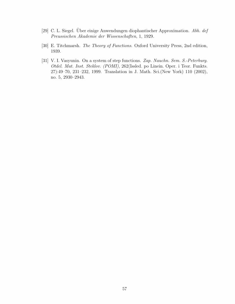
[29] C. L. Siegel. Uber einige Anwendungen diophantischer Approximation. Abh. defPreussischen Akademie der Wissenschaften, 1, 1929.
[30] E. Titchmarsh. The Theory of Functions. Oxford University Press, 2nd edition,1939.
[31] V. I. Vasyunin. On a system of step functions. Zap. Nauchn. Sem. S.-Peterburg.Otdel. Mat. Inst. Steklov. (POMI), 262(Issled. po Linein. Oper. i Teor. Funkts.27):49–70, 231–232, 1999. Translation in J. Math. Sci.(New York) 110 (2002),no. 5, 2930–2943.
57