instruction manual for concept simulators - john loomis · instruction manual for concept...

Instruction Manual for Concept Simulators

that accompany the book

Signals and Systems

by

M. J. Roberts

March 2004 - All Rights Reserved

Table of Contents I. Loading and Running the Simulators II. Continuous-Time Function Transformations III. Discrete-Time Function Transformations IV. Discrete-Time Convolution V. Continuous-Time Convolution VI. Fourier Methods VII. Excitation and Response of a Linear Time-Invariant

System using Fourier Methods VIII. Filters IX. Modulation/Demodulation X. Sampling XI. Transition from the Continuous-Time Fourier Transform (CTFT) to the Discrete Fourier Transform (DFT) XII. Continuous-Time Correlation XIII. Continuous-Time Feedback System Analysis

XIV. Discrete-Time Feedback System Analysis

Abbreviations and Acronyms CT Continuous Time DT Discrete Time CTFS Continuous-Time Fourier Series CTFT Continuous-Time Fourier Transform DTFS Discrete-Time Fourier Series DTFT Discrete-Time Fourier Transform DFT Discrete Fourier Transform

I. Loading and Running the Simulators All the concept simulators are MATLAB programs. They are written to run under MATLAB 6.5 or MATLAB 7.0 on Windows and under MATLAB 6.5 on UNIX or MAC OS X platforms. Each simulator is a “.p” file.

To run a simulator, load the .p file into a folder in the MATLAB path or add the folder where these files are to the MATLAB path. Then, at the MATLAB prompt (>>) type the name of the simulator, without an extension, for example, >>FilterDemo and then press the return (or enter) key. After a few seconds the simulator user interface (described below) should appear on the screen, ready for use. These simulators were written under MATLAB 6.5.1 or MATLAB 7.0. They may run under an other versions but that is definitely not guaranteed.

II. Continuous-Time Function Transformations The continuous-time (CT) function transformation concept simulator is the MATLAB p-code file, CTFns.p, located either in the Windows folder or the Macintosh folder depending on the operating system being used. This concept simulator illustrates concepts found on pages 22-66 in Signals and Systems by Roberts.

The purpose of the concept simulator is to allow students in Signals and Systems to generate many different kinds of continuous-time signals in pairs, amplitude-scale, time-shift and time-scale each of them individually, view a graph of each of them and also graph their sum and product. When the concept simulator is run a user interface screen appears.

The exact appearance of the screen will be slightly different on different platforms but the functions are always the same. The user interface consists of an array of buttons and sliders to control the simulator and graphs to illustrate the results. The top part of the user interface is divided into two halves, side-by-side. Each of them controls one signal. In each half are the following controls and displays.

1. Signal Function Selection Buttons This array of buttons allow the user to select the general type of signal function to be displayed.

Each button has on it a graphical symbol representing the type of function. They are, in order, sine, cosine, exponential, step, signum, ramp, impulse, comb, rectangle, triangle, sinc and dirichlet. 2. Signal Prototype Display To the upper right in each signal area is a graphical prototype of the function currently selected. It illustrates the general shape of the function and the meaning of the parameters which control it. In the example below it illustrates the meaning of the two parameters, A, the signal amplitude and

T0, the fundamental period.

3. Below the signal prototype is the name of the currently-selected signal and a scaled graph of it with the currently-selected parameter values.

4. Below the signal graph is a set of 2 to 4 sliders which can be used to adjust the parameter values which control the exact shape of the signal.

One the bottom 30% of the screen are two displays, the sum of the two signals on the left and the product on the right.

When any signal button is pressed or any parameter slider is adjusted, the displays of all affected signals are refreshed. When the signal selection is changed, the sliders are automatically changed to reflect that function’s parameters. When a new signal is selected, its parameters are always reset to its default values. The ranges of adjustment of parameters are intentionally constrained to lie within limits which allow the user to observe the effects of the various shifting and scaling transformations but do not allow adjustments covering more than an order of magnitude. This is done to keep the graphical displays simple and obvious, facilitating a quick, intuitive understanding of the effect of a parameter change.

III. Discrete-Time Function Transformations The discrete-time (DT) function transformation concept simulator is the MATLAB p-code file, DTFns.p, located either in the Windows folder or the Macintosh folder depending on the operating system being used. This concept simulator illustrates concepts found on pages 67-89 in Signals and Systems by Roberts.

The purpose of the concept simulator is to allow students in Signals and Systems to generate many different kinds of DT signals in pairs, amplitude-scale, time-shift and time-scale them , view a graph of each of them and also graph their sum and product. When the concept simulator is run a user interface screen appears.

The exact appearance of the screen will be slightly different on different platforms but the functions are always the same. The user interface consists of an array of buttons and sliders to control the simulator and graphs to illustrate the results. The top part of the user interface is divided into two halves, side-by-side. Each of them controls one signal. In each half are the following controls and displays. 1. Signal Function Selection Buttons

This array of buttons allows the user to select the general type of signal function to be displayed.

Each button has on it a graphical symbol representing the type of function. They are, in order, sine, cosine, exponential, sequence, signum, ramp, impulse, comb, rectangle, triangle, sinc and dirichlet. 2. Signal Prototype Display To the upper right in each signal area is a graphical prototype of the function currently selected. It illustrates the general shape of the function and the meaning of the parameters which control it. In the example below it illustrates the meaning of the two parameters, A, the signal amplitude and

N0, the fundamental period.

3. Below the signal prototype is the name of the currently-selected signal and a scaled graph of it with the currently-selected parameter values.


One the bottom 30% of the screen are two displays, the sum of the two signals on the left and the product on the right.

When any signal button is pressed or any parameter slider is adjusted, the displays of all affected signals are refreshed. When the signal selection is changed, the sliders are automatically changed to reflect that function’s parameters. When a new signal is selected, its parameters are always reset to its default values. The ranges of adjustment of parameters are intentionally constrained to lie within limits which allow the user to observe the effects of the various shifting and scaling transformations but do not allow adjustments covering more than an order of magnitude. This is done to keep the graphics displays simple and obvious, facilitating a quick, intuitive understanding of the effect of a parameter change.

IV. Discrete-Time Convolution The DT convolution concept simulator is a MATLAB p-code file, DTConv.p, located either in the Windows folder or the Macintosh folder depending on the operating system being used. This concept simulator illustrates concepts found on pages 151-170 in Signals and Systems by Roberts.

The purpose of the concept simulator is to allow students in Signals and Systems to generate many different kinds of DT signals in pairs, amplitude-scale, time-shift and time-scale them, view a graph of each of them and also observe their convolution. When the concept simulator is run a user interface screen appears.

The exact appearance of the screen will be slightly different on different platforms but the functions are always the same. The user interface consists of an array of buttons and sliders to control the demonstration and graphs to illustrate the results. The top part of the user interface is divided into two halves, side-by-side. Each of them controls one signal. In each half are the following controls and displays.


Each button has on it a graphical symbol representing the type of function. They are, in order, top to bottom, sine, cosine, exponential, sequence, signum, ramp, impulse, comb, rectangle, triangle, sinc and dirichlet. 2. Signal Prototype Display To the upper right in each signal area is a graphical prototype of the function currently selected. It illustrates the general shape of the function and the meaning of the parameters which control it. In the example below it illustrates the meaning of the three parameters, A, the signal amplitude,

n0, its time shift and

Nw

, its width parameter.

3. Below the signal prototype is a scaled graph of the currently-selected signal with the currently-selected parameter values.



One the bottom 40% of the screen are two displays. The left display shows the two signals plotted on the same scale at the top

and the product of the two signals below that.

(In this example, at this shift, the product is zero everywhere.) Below that are the controls to start the convolution process and to control the speed with which it proceeds.

When the user presses the “Convolve” button, the concept simulator illustrates convolution by animating the two signals, their product, and the resulting convolution. The signal from the left side of the screen is

g1 n[ ] and the signal from the right side of the screen is

g2 n[ ] . The two signals,

g1 m[ ] and

g2 n ! m[ ] are plotted versus

m ,

g1 m[ ] in red and static and

g2 n ! m[ ] in blue and moving left-to-right as n is varied from -10 to +10. As n is varied, its value is reported below. At the same time, in the product graph the product of the two signals,

g1 m[ ]g2 n ! m[ ] is plotted in black on the same

m scale. The sum of that product is the convolution of the two signals. That sum is plotted simultaneously as a function of n in the lower right-hand side of the screen.

V. Continuous-Time Convolution The CT convolution concept simulator is a MATLAB p-code file, CTConv.p, located either in the Windows folder or the Macintosh folder depending on the operating system being used. This concept simulator illustrates concepts found on pages 170-189 in Signals and Systems by Roberts.

The purpose of the concept simulator is to allow students in Signals and Systems to generate many different kinds of CT signals in pairs, amplitude-scale, time-shift and time-scale them, view a graph of each of them and also observe their convolution. When the concept simulator is run a user interface screen appears.

The exact appearance of the screen will be slightly different on different platforms but the functions are always the same. The user interface consists of an array of buttons and sliders to control the demonstration and graphs to illustrate the results. The top part of the user interface is divided into two halves, side-by-side. Each of them controls one signal. In each half are the following controls and displays.


Each button has on it a graphical symbol representing the type of function. They are, in order, top to bottom, sine, cosine, exponential, step, signum, ramp, impulse, comb, rectangle, triangle, sinc and dirichlet. 2. Signal Prototype Display To the upper right in each signal area is a graphical prototype of the function currently selected. It illustrates the general shape of the function and the meaning of the parameters which control it. In the example below it illustrates the meaning of the three parameters, A, the signal amplitude,

t0, its time shift and w, its width.

3. Below the signal prototype is a scaled graph of the currently-selected signal with the currently-selected parameter values.



One the bottom 40% of the screen are two displays. The left display shows the two signals plotted on the same scale at the top

and the product of the two signals below that.

Below that are the controls to start the convolution process and to control the speed with which it proceeds.

When the user presses the “Convolve” button, the concept simulator illustrates convolution by animating the two signals, their product, and the resulting convolution. The signal from the left side of the screen is

g1 t( ) and the signal from the right side of the screen is

g2 t( ) . The two signals,

g1 !( ) and

g2 t !"( ) are plotted versus

! ,

g1 !( ) in red and static and

g2 t !"( ) in blue and moving left-to-right as t is varied from -2 to +2. As t is varied, its value is reported below. At the same time, in the product graph the product of the two signals,

g1 !( )g2 t" !( ) is plotted in black on the same

! scale. The area under that product is the convolution of the two signals. That area is plotted simultaneously as a function of t in the lower right-hand side of the screen.

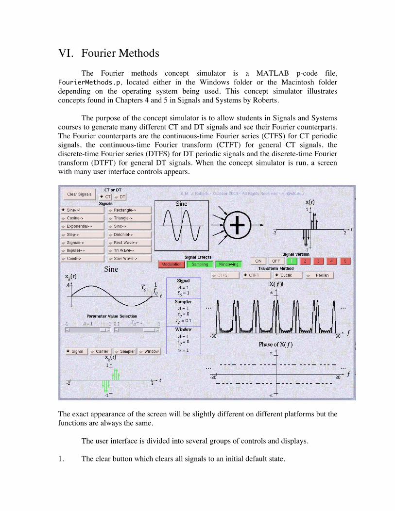
VI. Fourier Methods The Fourier methods concept simulator is a MATLAB p-code file, FourierMethods.p, located either in the Windows folder or the Macintosh folder depending on the operating system being used. This concept simulator illustrates concepts found in Chapters 4 and 5 in Signals and Systems by Roberts.

The purpose of the concept simulator is to allow students in Signals and Systems courses to generate many different CT and DT signals and see their Fourier counterparts. The Fourier counterparts are the continuous-time Fourier series (CTFS) for CT periodic signals, the continuous-time Fourier transform (CTFT) for general CT signals, the discrete-time Fourier series (DTFS) for DT periodic signals and the discrete-time Fourier transform (DTFT) for general DT signals. When the concept simulator is run, a screen with many user interface controls appears.

The exact appearance of the screen will be slightly different on different platforms but the functions are always the same.

The user interface is divided into several groups of controls and displays. 1. The clear button which clears all signals to an initial default state.

2. The CT and DT buttons which choose whether CT or DT signals will be generated.

3. The signal buttons which choose which types of signals are to be generated. There are fourteen types of functions for CT signals and another 14 for DT signals. The button titles also indicate which versions of each signal function are currently active. For example, in the figure below, (a windowed and sampled) Sine #1 is currently active.

4. The signal generator diagram which graphically indicates the currently-selected function which can be added to the overall signal. The presence of multiple arrows entering the summer indicates that the current signal is just one of many which may be added to produce an overall signal.

5. Below the signal buttons is the prototype function display which shows the general shape of the currently selected function and indicates graphically the parameters which control its form. The ordinate is labeled,

xkt( ) , to indicate symbolicallly that it is

the “kth” signal of a set of signals which are added to form the overall signal.

6. Directly below the prototype function display is a group of two to four “sliders” which allow the user to directly adjust the parameters of the current version of the currently-selected signal function (or the parameters controlling the way it is modulated, sampled or windowed) over a limited range.

7. Below the sliders is a set of four buttons that select which set of parameters the sliders control, the signal function, the sinusoidal carrier it can modulate, the sampler which can impulse sample it or the window which can window it.

8. Below these four buttons is a graphical display of the current version of the currently-selected signal function, as modulated, sampled and/or windowed, if these effects are applied. In this example, the currently-selected signal is a sine function and it is both windowed and sampled. Its green color indicates that it is currently active. A currently inactive signal is displayed in red.

9. In the upper right-hand corner is a display of the overall signal. This signal is the sum of all the versions of all the signals that are currently active. In this example only one signal is active so the overall signal and the currently-selected signal version are the same.

10. Below the overall signal display are an “ON” button, and “OFF” button and five signal “version” buttons numbered one through five. The current version of the currently-selected signal can be turned on (activated) or turned off (deactivated) by the ON and OFF buttons. Each signal function can be generated in up to five different forms with different parameters, each of which can be turned on and added to the overall signal. That makes a total of 70 signals that can be added, 5 versions of each of 14 signal functions.

The green color of button number #1 in the illustration indicates that version number one is currently active. The large white numeral “1” compared with the smaller black numerals “2”, “3”, “4” and “5” indicates that version #1 is also currently selected for parameter variation. 11. To the left of the ON, OFF and version buttons is a set of three buttons which turn on or off three signal effects, modulation, (impulse) sampling and windowing for the current version of the currently-selected signal function.

12. Below the ON, OFF and version buttons are four buttons which control which Fourier method is applied and how it is displayed. In the CT mode, they are CTFS, CTFT, Cyclic and Radian.

The “Cyclic” button sets the display of a CTFT to be a function of cyclic frequency, f. The “Radian” button sets the display of a CTFT to be a function of radian frequency, ω. When CTFS is chosen these two buttons are disabled. CTFS can only be chosen when the overall signal is periodic. When the overall signal is aperiodic only the CTFT can be displayed. In the DT mode, the display options are DTFS, DTFT, Cyclic and Radian. The “Cyclic” button sets the display of a DTFT to be a function of cyclic DT frequency, F. The “Radian” button sets the display of a DTFT to be a function of radian DT frequency, Ω. When DTFS is chosen these two buttons are disabled. DTFS can only be chosen when the overall signal is periodic. When the overall signal is aperiodic only the DTFT can be displayed. 13. In the lower right-hand corner are two areas for the graphs of the magnitude and phase of the CTFS, CTFT, DTFS or DTFT.

14. In the lower middle of the screen is a display of all the values of all the parameters which apply to the current version of the currently-selected signal function.

The operation of the concept simulator is intended to be simple and intuitive, once the control functions are understood. The user may activate or deactivate any version of any signal by first selecting it using the signal and version buttons and then clicking on ON or OFF. Every time any signal is changed, the displays of the current signal version, the overall signal, the magnitude and phase of the CTFS, CTFT, DTFS or DTFT and the signal parameter list are updated. All parameters for all versions of all signals are remembered. So if a certain signal effect is set up for a certain signal version and then other signals are adjusted, when the user returns to the original version of the original signal, the parameter values and effects are still there. All parameters have limited ranges. There are two reasons. First it simplifies the graphics, allowing most graphs to have fixed scales. This makes an intuitive and direct comparison of effects easier. Also, this concept simulator is not intended to be an all purpose Fourier-transform or Fourier-series calculation machine. It is simply intended to reinforce concepts and to help a student see how an effect in the time domain creates a corresponding effect in the frequency (or harmonic number) domain.

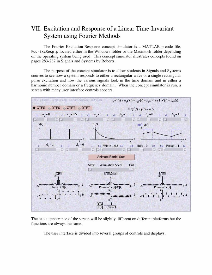
VII. Excitation and Response of a Linear Time-Invariant System using Fourier Methods

The Fourier Excitation-Response concept simulator is a MATLAB p-code file, FourExcResp.p located either in the Windows folder or the Macintosh folder depending on the operating system being used. This concept simulator illustrates concepts found on pages 283-287 in Signals and Systems by Roberts.

The purpose of the concept simulator is to allow students in Signals and Systems courses to see how a system responds to either a rectangular wave or a single rectangular pulse excitation and how the various signals look in the time domain and in either a harmonic number domain or a frequency domain. When the concept simulator is run, a screen with many user interface controls appears.

The exact appearance of the screen will be slightly different on different platforms but the functions are always the same.

The user interface is divided into several groups of controls and displays.

1. At the upper left-hand corner is a set of four buttons which control the type of Fourier analysis to be done. Continuous-Time Fourier Series - CTFS Discrete-Time Fourier Series - DTFS Continuous-Time Fourier Transform - CTFT Discrete-Time Fourier Transform - DTFT

As shown here CTFS is currently selected. 2. At the upper right-hand corner is an area in which a prototypical differential or difference equation is displayed with coefficients,

a2,a1,a0,b2,b1,b0. Below that is a

display of the same equation but with the currently-selected values of the coefficients.

Differential Equation

Difference Equation

3. Just below the Fourier-method selection buttons and the differential or difference equation display is a group of 6 sliders which allow the user to set the values of the coefficients,

a2,a1,a0,b2,b1,b0.

As the coefficients are changed the system dynamics change.

4. Just below the coefficient sliders are three graphs, the excitation, the impulse response and the system response all as functions of time, continuous or discrete.

Continuous-Time Signals

Discrete-Time Signals

Every time a coefficient or an excitation parameter is changed, these graphs change accordingly. 5. Below the time-domain signal displays is a set of 5 sliders which allow the user to set the parameters which determine the exact shape of the excitation.

A1 One level of the rectangular wave or rectangular pulse

A2 The other level of the rectangular wave or rectangular pulse

Width The width of the rectangular wave or rectangular pulse at level

A1

Shift The shift of the rectangular wave or rectangular pulse Period The period of the rectangular wave (disabled for rectangular pulses) 6. Below the excitation waveform parameter sliders in the middle of the screen is an area containing a button “Animate Partial Sum” which initiates an animation showing the build-up of the exctitation and response one Fourier series harmonic function at a time. Below that button is a slider which is used to control the speed of the animation.

When the animation appears, the excitation partial sum is to the left of this area and the response partial sum is to the right. Animation is only used for Fourier series analysis, not Fourier transform analysis. 7. Below the animation control area are 3 pairs of graphs, magnitude above phase, for the excitation, transfer function and response in either the harmonic number or frequency domain.

Signal Display in the Harmonic Number (k) Domain

Signal Display in the CT Frequency ( f ) Domain

Signal Display in the DT Frequency ( F ) Domain

8. At the bottom of the screen is an area in which the transfer function of the system is displayed in analytical form.

CTFS Transfer Function DTFS Transfer Function

CTFT Transfer Function in f and ω forms

DTFT Transfer Function in F and Ω forms

VIII. Filters The Filter concept simulator is a MATLAB p-code file, FilterDemo.p, located either in the Windows folder or the Macintosh folder depending on the operating system being used. This concept simulator illustrates concepts found on pages 395-417 in Signals and Systems by Roberts (and, to some extent, material found on pages 720-725).

The purpose of the concept simulator is to allow students in Signals and Systems to excite various kinds of filters with a selection of typical signal types, to see the excitation and response signals in both the time and frequency domains and to hear both signals. When the concept simulator is run, a screen with many user interface controls and displays appears

The user interface is divided into several groups of controls and displays. 1. In the upper left-hand corner is a set of four buttons used to determine the kind of excitation signal, a sinusoid (a sine wave), a rectangular wave with an average value of zero and a duty cycle that can be set by the user, a triangular wave or a bandlimited white noise (random) signal.

2. Below these buttons are some sliders which are used to set excitation signal parameters. There are four in all, but at any one time only those which are needed are visible. They set the fundamental frequency of the excitation (if it is periodic), the duty cycle (if it is a rectangular wave) and the lower and upper frequency limits on its bandwidth (if it is bandlimited white noise).

The lower and upper frequency limits are constrained by the software such that the lower frequency is always at least 100 Hz below the upper frequency. That is, if the upper frequency is set below the current value of the lower frequency, the lower frequency is changed to a lower value.

3. In the upper middle of the screen are the controls for modulation. Any of the signals can also be used to modulate either a sinusoid (double-sideband suppressed-carrier modulation) or a rectangular pulse wave (natural pulse-amplitude modulation) to form the overall excitation signal.

When modulation is turned off, the two lower buttons are still visible but disabled. 4. Below the modulation control buttons are two sliders which control the fundamental frequency of the modulation and (if it is a rectangular pulse wave) the duty cycle. In this case the pulse wave does not have an average value of zero but instead is always non-negative with a maximum value of one and a minimum value of zero.

5. In the upper right-hand corner of the screen are buttons which control what type of filtering is to be done. The filter can be ideal or Butterworth and can be lowpass,

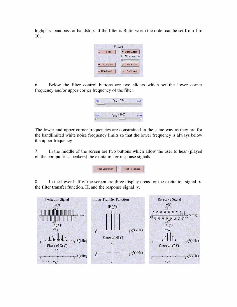
highpass, bandpass or bandstop. If the filter is Butterworth the order can be set from 1 to 10.

6. Below the filter control buttons are two sliders which set the lower corner frequency and/or upper corner frequency of the filter.

The lower and upper corner frequencies are constrained in the same way as they are for the bandlimited white noise frequency limits so that the lower frequency is always below the upper frequency.

7. In the middle of the screen are two buttons which allow the user to hear (played on the computer’s speakers) the excitation or response signals.

8. In the lower half of the screen are three display areas for the excitation signal, x, the filter transfer function, H, and the response signal, y.

IX. Modulation/Demodulation

The Modulation/Demodulation concept simulator is a MATLAB p-code file, Modulation.p, located either in the Windows folder or the Macintosh folder depending on the operating system being used. This concept simulator illustrates concepts found on pages 448-456 in Signals and Systems by Roberts.

The purpose of the concept simulator is to allow students in Signals and Systems to simulate various kinds of continuous-time modulation and demodulation and to see all the signals that result in both the time and frequency domains. When the concept simulator is run, a screen with many user interface controls and displays appears.

The user interface is divided into several groups of controls and displays.

1. In the upper left-hand corner is a set of three modulation buttons. DSBSC - Double-Sideband Suppressed-Carrier DSBTC - Double-Sideband Transmitted-Carrier SSBSC - Single-Sideband Suppressed-Carrier

2. To the right of the modulation buttons is a set of two demodulation buttons. Synchronous - Synchronous demodulation using a local oscillator Envelope - Asynchronous demodulation using an envelope detector

3. Below the modulation and demodulation buttons is a diagram of the communication system being simulated. The information signal,

x t( ) , modulates a cosine carrier to form the transmitted signal,

ytt( ) . The transmitted signal,

ytt( ) , is

demodulated by either synchronous or asynchronous detection to form

ydt( ) . The

demodulated signal,

ydt( ) , is lowpass filtered to remove images at twice the carrier

frequency (if present) to form

yLPt( ) . Finally, the lowpass filtered signal,

yLPt( ) , is

highpass filtered to remove any “dc” component that might be present to form

yHP

t( ) .

4. Below the system diagram are the display areas for the five signals. (In the examples below the modulation is DSBSC and the demodulation is synchronous.) The information signal, in the time and frequency domains, is graphed in red. The information signal is a bandlimited white noise signal generated randomly every time a button is pressed.

The transmitted signal, in the time and frequency domains, is graphed in green, with the information signal superimposed in red in the time domain for comparison.

The demodulated signal, in the time and frequency domains, is graphed in blue, with the information signal superimposed in red in the time domain for comparison.

The lowpass filtered signal, in the time and frequency domains, is graphed in purple, with the information signal superimposed in red in the time domain for comparison.

The highpass filtered signal, in the time and frequency domains, is graphed in black, with the information signal superimposed in red in the time domain for comparison.

X. Sampling The Sampling concept simulator is a MATLAB p-code file, Sampling.p, located either in the Windows folder or the Macintosh folder depending on the operating system being used. This concept simulator illustrates concepts found on pages 496-525 in Signals and Systems by Roberts.

The purpose of the concept simulator is to allow students in Signals and Systems to sampling various kinds of energy and periodic power signals and see the transforms in continuous-time and discrete time and compare them to develop an intuitive understanding of the sampling process.

When the concept simulator is run, a screen with many user interface controls and displays appears.

The user interface is divided into several groups of controls and displays. 1. In the upper left-hand corner is a pop-up menu which allows the user to select any one of 9 signals, sine, cosine, exponential, rectangle, triangle, sinc, rectangular wave, triangular wave and dirichlet. This is the continuous-time signal that will be sampled.

2. To the right of the signal-selection menu is a set of four sliders, each of which sets the value of a signal parameter. Not all signals use all sliders and, when a signal does not use a slider, it is made invisible.

The leftmost slider sets the amplitude, A, of the signal. The second slider sets the fundamental frequency,

f0, of the signal (if it is periodic). The third slider sets the time

shift,

t0, of the signal. The fourth slider has multiple purposes. It sets the width, w, of

rectangle, triangle and sinc signals. It sets the time constant, τ, of the exponential signal. It sets the duty cycle,

w /T0, (pulse width divided by period) of the rectangular wave and

triangular wave signals. And it sets the order, N, of the dirichlet signal. 3. Just below the signal-parameter sliders on the right-hand side of the screen are three sliders which control the sampling process. The left-hand slider sets the sampling rate,

fs, the middle slider sets the discrete time of the first sample and the right-hand slider sets the number of samples, N.

4. On the left side of the screen, just below the signal-selection pop-up menu is a plot of a prototype of the signal selected. Its purpose is to define graphically the parameters which control the signal.

5. Just below the prototype plot is a time-domain plot of the currently-selected continuous-time signal,

x t( ) and the discrete-time signal,

x n[ ] , formed by sampling it.

The red plot is

x t( ) and the blue plot is

x n[ ] .

x t( ) is plotted versus continuous-time, t, and

x n[ ] is “stem” plotted versus the product,

nTs, of discrete time, n, and the time

between samples,

Ts. This allows the use of a single time scale and direct comparison of

the two signals.

6. Below the time-domain signal plot are two control buttons. They set the frequency-domain plot to be plotted as a function of either cyclic frequency, f, or radian frequency, ω.

8. Below the Cyclic/Radian buttons are plots of the magnitude and phase of the continuous-time Fourier transform (CTFT) of

x t( ) ,

X f( ) or

X j!( ) .

9. To the right of the Cyclic/Radian buttons are three buttons which set the display of the discrete-time transform of the discrete-time signal,

x n[ ] .

The DTFS button sets the display to be the discrete-time Fourier series harmonic function of

x n[ ] ,

X k[ ] , a function of discrete harmonic number, k. The ~CTFS button sets the display to be an approximation of the CTFS of the continuous-time signal,

x t( ) , based on the N samples in

x n[ ] . This approximation is

X k[ ] plotted versus

kfs /N . If the signal is periodic and bandlimited and the sampling exactly covers an integer number of cycles of

x t( ) , this plot is exact. The last button, ~CTFT, sets the display to be an approximation of the CTFT,

X f( ) , of the signal,

x t( ) . This works best for energy signals. Although it can never be exact, with a high sampling rate and a large number of points this

approximation can be quite accurate for low frequencies (well below half the sampling rate). 10. Below the three buttons, DTFS, ~CTFS and ~CTFT, are plots of the magnitude and phase of the type of transform of the discrete-time signal,

x n[ ] , selected by those three buttons.

XI. Transition from the Continuous-Time Fourier Transform (CTFT) to the Discrete Fourier Transform (DFT) The CTFT-to-DFT concept simulator is a MATLAB p-code file, DFT.p, located either in the Windows folder or the Macintosh folder depending on the operating system being used. This concept simulator illustrates concepts found on pages 525-535 in Signals and Systems by Roberts.

The purpose of the concept simulator is to demonstrate to students in Signals and Systems the relationship between the CTFT of a continuous-time signal and the DFT of a finite-length set of samples from that signal through the operations of time-domain sampling, time-domain windowing and frequency-domain sampling. When the concept simulator is run, a screen with many user interface controls and displays appears.

The user interface is divided into several groups of controls and displays. 1. In the upper left-hand corner is a pop-up menu which allows the user to select the type of signal to be used in the demonstration, Sine, Cosine, Exponential, Rectangle, Triangle, Sinc, Rectangular Wave, Triangular Wave or Dirichlet.

2. To the right of the signal-selection menu is a set of four sliders, each of which allows the user to set the value of a signal parameter. For any given signal, only those sliders which control parameters relevant to it are displayed. The others are made invisible.

The leftmost slider sets the amplitude, A, of the signal. The second slider sets the fundamental frequency,

f0, of the signal (if it is periodic). The third slider sets the time

shift,

t0, of the signal. The fourth slider has multiple purposes. It sets the width, w, of

rectangle, triangle and sinc signals. It sets the time constant, τ, of the exponential signal. It sets the duty cycle,

w /T0, (pulse width divided by period) of the rectangular wave and

triangular wave signals. And it sets the order, N, of the dirichlet signal. 3. Below the signal-parameter sliders is a set of two sliders which control the sampling process. The left slider sets the sampling rate and the right slider sets the number of samples. The first sample is always taken at time,

t = 0 .

4. To the left of the sampling-parameter sliders and below the signal-selection menu is a display of a prototype of the signal currently selected. The prototype graphically defines the parameters which determine the signal.

5. The bottom two-thirds of the screen has eight graphs, four in the continuous or discrete time domain and four in the frequency or harmonic-number domain.

At the top are the original continuous-time signal on the left and the magnitude of its CTFT on the right. Below the continuous-time signal is the discrete-time signal formed by sampling the continuous-time signal and to its right is the magnitude of its DTFT. Sampling in the time domain corresponds to periodic repetition in the frequency domain. Below the discrete-time signal is a windowed version of it which has only a finite number of non-zero values. To its right is its DTFT. Windowing in the time corresponds to convolution with the DTFT of the window function in the discrete-time frequency domain. Below the DTFT of the windowed signal is a frequency sampled version of it. This frequency-sampled DTFT is the DFT of the discrete-time signal graphed to its left. Sampling in the discrete-time frequency domain corresponds to periodic repetition in the discrete-time harmonic number domain. XII. Continuous-Time Correlation The Continuous-time Correlation concept simulator is a MATLAB p-code file, CTCorr.p, located either in the Windows folder or the Macintosh folder depending on the operating system being used. This concept simulator illustrates concepts found on pages 573-605 in Signals and Systems by Roberts.

The purpose of the concept simulator is to demonstrate to students in Signals and Systems relationships between continuous-time signals through the correlogram and the correlation function When the concept simulator is run, a screen with many user interface controls and displays appears.

The user interface is divided into several groups of controls and displays. 1. In the upper left-hand and upper right-hand corners are two menus which allow the user to select the type of signals, x and y, to be generated, Sine, Cosine, Exponential, Rectangle, Triangle, Sinc, Rectangular Wave, Triangular Wave, Dirichlet or Random.

As illustrated here, a sine and a cosine have been selected. 2. In the upper middle of the screen is an area entitled “Correlogram”. Here a correlogram of the two signals is graphed. The correlogram can be either static or dynamic. When two signals are first chosen the correlogram is static, showing the relationship between the signals with both signals unshifted. When the user presses the “Correlate” buttton (described below) the correlogram is animated to show the relationship between the signals as one of them is shifted.

The correlogram illustrated here is for two uncorrelated random signals. 3. Just below each menu are two graphs, a prototype of the signal selected, to graphically define its parameters, and a scaled graph of the currently-selected signal with the current parameter values.

4. Below each prototype- graph pair is a set of sliders which are used to set parameter values. There can be up to four sliders and, if fewer than four sliders are needed for any particular signal, only the sliders needed are shown.

In this illustration three sliders are shown to set the amplitude, period and time shift of a sinusoid. The signals and their associated parameters are summarized in the table below. Sine Amplitude Period Time Shift Cosine Amplitude Period Time Shift Exponential Amplitude Time Shift Time Constant Rectangle Amplitude Time Shift Width Triangle Amplitude Time Shift Width Sinc Amplitude Time Shift Width Rectangular Wave Amplitude Period Time Shift Duty Cycle Triangular Wave Amplitude Period Time Shift Duty Cycle Dirichlet Amplitude Period Time Shift Order, N Random Signal Std. Dev. Low-Freq Corner Hi-Freq Corner

5. In the middle of the screen are a “Correlate” button and an associated slider.

The Correlate button initiates an animation of the correlation between the two functions, x and y, as y is shifted. The slider controls the speed of the animation. 6. At the lower left of the screen are two graphs which are animated when the Correlate button is pressed. The upper graph shows the two functions being correlated, with x static and y shifting. The x signal is shown as a solid blue curve and the y signal is shown as a dashed blue curve. The lower graph shows the product of x and y as y is shifted, graphed as a red curve.

As the y signal is shifted, a text annotation of the form, “

! = xxx ” shifts along with the y signal, always indicating numerically the amount of time shift. There are two vertical black-line markers to establish the time scale of the graphs. If both x and y are periodic, these two markers delimit one common period for the two signals. If either signal is not periodic these markers simply serve to set the time scale. 7. In the lower right-hand corner of the screen is a graph of the cross correlation function,

R xy !( ) . As the y signal is shifted, the cross correlation function is also animated to show the development of the function with shift.

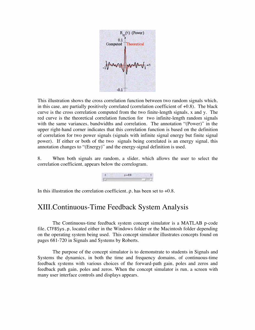
This illustration shows the cross correlation function between two random signals which, in this case, are partially positively correlated (correlation coefficient of +0.8). The black curve is the cross correlation computed from the two finite-length signals, x and y. The red curve is the theoretical correlation function for two infinite-length random signals with the same variances, bandwidths and correlation. The annotation “(Power)” in the upper right-hand corner indicates that this correlation function is based on the definition of correlation for two power signals (signals with infinite signal energy but finite signal power). If either or both of the two signals being correlated is an energy signal, this annotation changes to “(Energy)” and the energy-signal definition is used. 8. When both signals are random, a slider, which allows the user to select the correlation coefficient, appears below the correlogram.

In this illustration the correlation coefficient, ρ, has been set to +0.8. XIII. Continuous-Time Feedback System Analysis The Continuous-time feedback system concept simulator is a MATLAB p-code file, CTFBSys.p, located either in the Windows folder or the Macintosh folder depending on the operating system being used. This concept simulator illustrates concepts found on pages 681-720 in Signals and Systems by Roberts.

The purpose of the concept simulator is to demonstrate to students in Signals and Systems the dynamics, in both the time and frequency domains, of continuous-time feedback systems with various choices of the forward-path gain, poles and zeros and feedback path gain, poles and zeros. When the concept simulator is run, a screen with many user interface controls and displays appears.

The user interface is divided into several groups of controls and displays. 1. In the upper left-hand corner and in the lower left-hand corner are two displays, each containing a menu, a slider and a graph for setting and displaying poles, zeros and gains for the forward and feedback paths of the overall system.

The menu allows the user to select whether to add a pole to, add a zero to or remove a pole or zero from each system. The slider is used to set the gain of each system. The graph displays the pole and zero locations for each system. 2. Between the two pole-zero-gain setting areas is a diagram of the prototype feedback to illustrate the relationship between the individual systems and the overall system.

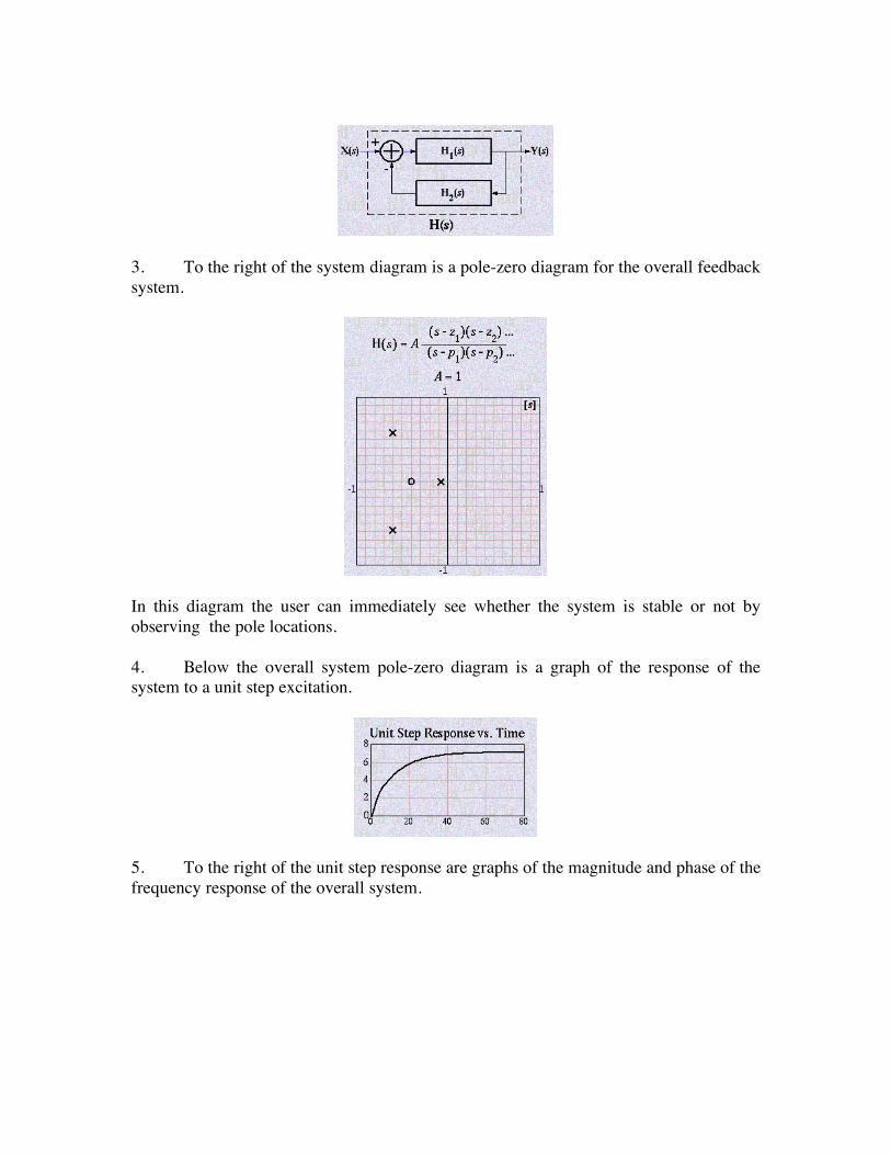
3. To the right of the system diagram is a pole-zero diagram for the overall feedback system.

In this diagram the user can immediately see whether the system is stable or not by observing the pole locations. 4. Below the overall system pole-zero diagram is a graph of the response of the system to a unit step excitation.

5. To the right of the unit step response are graphs of the magnitude and phase of the frequency response of the overall system.

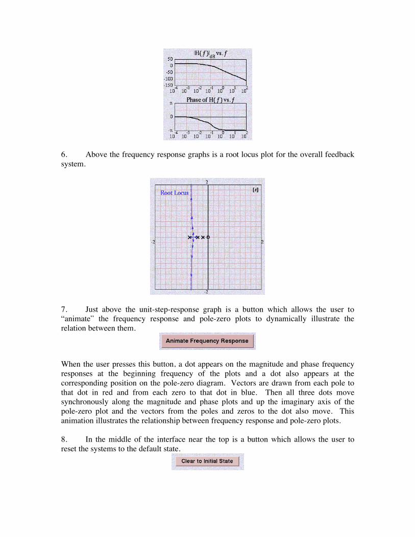
6. Above the frequency response graphs is a root locus plot for the overall feedback system.

7. Just above the unit-step-response graph is a button which allows the user to “animate” the frequency response and pole-zero plots to dynamically illustrate the relation between them.

When the user presses this button, a dot appears on the magnitude and phase frequency responses at the beginning frequency of the plots and a dot also appears at the corresponding position on the pole-zero diagram. Vectors are drawn from each pole to that dot in red and from each zero to that dot in blue. Then all three dots move synchronously along the magnitude and phase plots and up the imaginary axis of the pole-zero plot and the vectors from the poles and zeros to the dot also move. This animation illustrates the relationship between frequency response and pole-zero plots. 8. In the middle of the interface near the top is a button which allows the user to reset the systems to the default state.

XIV. Discrete-Time Feedback System Analysis The Discrete-time feedback system concept simulator is a MATLAB p-code file, DTFBSys.p, located either in the Windows folder or the Macintosh folder depending on the operating system being used. This concept simulator illustrates concepts found on pages 800-816 in Signals and Systems by Roberts.

The purpose of the concept simulator is to demonstrate to students in Signals and Systems the dynamics, in both the time and frequency domains, of discrete-time feedback systems with various choices of the forward-path gain, poles and zeros and feedback path gain, poles and zeros. When the concept simulator is run, a screen with many user interface controls and displays appears.

The user interface is divided into several groups of controls and displays. 1. In the upper left-hand corner and in the lower left-hand corner are two displays, each containing a menu, a slider and a graph for setting and displaying poles, zeros and gains for the forward and feedback paths of the overall system.

The menu allows the user to select whether to add a pole to, add a zero to or remove a pole or zero from each system. The slider is used to set the gain of each system. The graph displays the pole and zero locations for each system. 2. Between the two pole-zero-gain setting areas is a diagram of the prototype feedback to illustrate the relationship between the individual systems and the overall system.

3. To the right of the system diagram is a pole-zero diagram for the overall feedback system.

In this diagram the user can immediately see whether the system is stable or not by observing the pole locations. 4. Below the overall system pole-zero diagram is a graph of the response of the system to a unit sequence excitation.

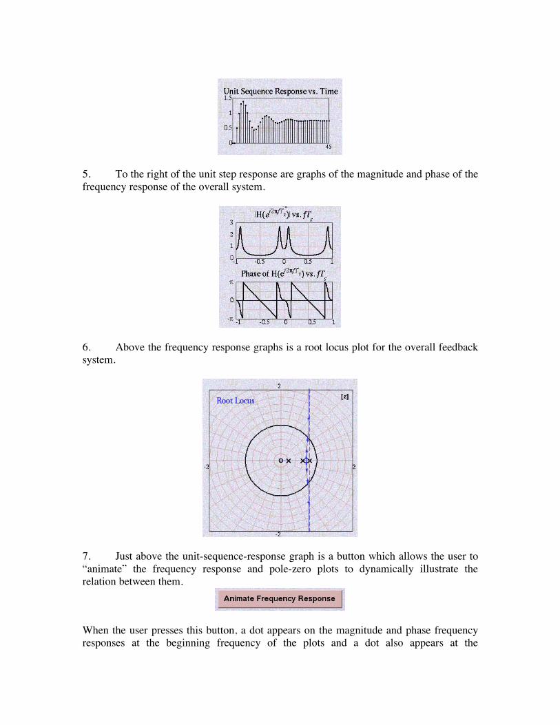
5. To the right of the unit step response are graphs of the magnitude and phase of the frequency response of the overall system.

6. Above the frequency response graphs is a root locus plot for the overall feedback system.

7. Just above the unit-sequence-response graph is a button which allows the user to “animate” the frequency response and pole-zero plots to dynamically illustrate the relation between them.

When the user presses this button, a dot appears on the magnitude and phase frequency responses at the beginning frequency of the plots and a dot also appears at the

corresponding position on the pole-zero diagram on the unit circle. Vectors are drawn from each pole to that dot in red and from each zero to that dot in blue. Then all three dots move synchronously along the magnitude and phase plots and around the unit circle of the pole-zero plot and the vectors from the poles and zeros to the dot also move. This animation illustrates the relationship between frequency response and pole-zero plots.

8. In the middle of the interface near the top is a button which allows the user to reset the systems to the default state.

instruction manual for concept simulators - john loomis · instruction manual for concept...

Documents