instituto de computaÇÃoreltech/2011/11-20.pdf · instituto de computaÇÃo universidade estadual...

�� INSTITUTO DE COMPUTAÇÃOUNIVERSIDADE ESTADUAL DE CAMPINAS

Multi-Scale Classification ofRemote Sensing Images

J. A. dos Santos P-H. GosselinS.Philipp-Foliguet R. da S. Torres

A. X. Falcão

Technical Report - IC-11-20 - Relatório Técnico

November - 2011 - Novembro

The contents of this report are the sole responsibility of the authors.O conteúdo do presente relatório é de única responsabilidade dos autores.

Multi-Scale Classification of Remote Sensing Images

Jefersson Alex dos Santos Philippe-Henri Gosselin Sylvie Philipp-FoliguetRicardo da S. Torres Alexandre Xavier alcao

Abstract

A huge effort has been applied in image classification to create high quality the-matic maps and to establish precise inventories about land cover use. The peculiaritiesof Remote Sensing Images (RSIs) combined with the traditional image classificationchallenges made RSIs classification a hard task. Our aim is to propose a kind of boost-classifier adapted to multi-scale segmentation. We use the paradigm of boosting, whoseprinciple is to combine weak classifiers to build an efficient global one. Each weak clas-sifier is trained for one level of the segmentation and one region descriptor. We haveproposed and tested weak classifiers based on linear SVM and region distances providedby descriptors. The experiments were performed on a large image of coffee plantations.We have shown in this paper that our approach based on boosting can detect the scaleand set of features best suited to a particular training set. We have also shown that hi-erarchical multi-scale analysis is able to reduce training time and to produce a strongerclassifier. We compare the proposed methods with a baseline based on SVM with RBFkernel. The results show that the proposed methods outperform the baseline.

1 Introduction

Since the satellite imagery information became accessible to the civil community in the1970s, a huge effort has been applied in image classification to create high quality thematicmaps and to establish precise inventories about land cover use [41]. However, the peculiar-ities of Remote Sensing Images (RSIs) combined with the traditional image classificationchallenges have turned RSIs classification into a hard task.

The use of RSIs as a source of information in agribusiness applications is very common.In those applications, it is fundamental to know how the space occupation is done. However,identification and recognition of crop regions in remote sensing images are not trivial tasksyet. In Brazil, for example, coffee is one of the most important agricultural cultures. In thiswork, which is part of a Brazilian project in collaboration with a cooperative organizationof coffee producers, we are interested in the analysis of RSI where these plantations can befound.

Apart from the typical RSI classification problems, there are some specific issues inagriculture. As far as the identification of coffee regions is concerned, there are some otherinterferences, since it is usually grown in mountainous regions (for example, in Brazil).This fact often causes shadows and distortions in the spectral information. Great difficultyarises in classification and interpretation of shaded objects in an image because their spectral

1

2 dos Santos et al.

information is either reduced or totally lost [44]. Moreover, the growing of coffee is not aseasonal activity, and, therefore, in the same region, there may be coffee plantations ofdifferent ages, which also affects the observed spectral patterns.

Typically, the classification process of RSIs uses supervised learning, which can be di-vided in the following components: data representation, feature extraction and training.Data representation indicates the objects for classification (e.g., pixels [32], blocks of pix-els [9], regions [1], and hierarchy of regions [5]). Feature extraction provides a mathematicaldescription for each object (for example, spectral characteristics, texture, shape). Traininglearns how to separate objects from distinct classes by building a classifier based on machinelearning techniques (for instance, support vector machines [37], genetic programming [9],neural networks [29]). The final quality of the classification depends on the performance ofeach step. For example, the classification result relies on the accuracy of the employed learn-ing techniques. Regarding the performance of learning algorithms, it is directly dependenton the quality of the extracted image features. Finally, features are extracted according tothe model used for data representation.

Regardless of the data representation model adopted in supervised classification of RSIs,both the training input and the result of the classifier can be expressed as sets of pixels. Inspite of it, data representation cannot rely only on pixels, because their image characteristicsare not usually enough to capture the patterns of the classes (regions of interest). In orderto improve that semantic gap, multi-scale image segmentation can play an important role.As pointed out by Trias-Sanz et al. [34], most image segmentation methods use thresholdparameters to create a partition of the image. These methods usually create a single-scalerepresentation of the image: small thresholds give segmentation with small regions andmany details while large thresholds preserve only the most salient regions. The problem isthat various structures can appear at different scales and this segmentation result can bedifficult to be obtained without prior knowledge about the data or by using only empiricalparameters. Some parts of an image may need a fine segmentation, since the plots aresmall, whereas, in other parts, a coarse segmentation is sufficient. For this reason, the maindrawback of classification methods based on regions is that they depend on the segmentationmethod used. Moreover, it is difficult to define the optimal scale segmentation. Bearingthis in mind, many researchers have exploited multiple scales of data [17, 19, 29, 35, 37, 39].

Allied to the problem of finding the best scale representation of segmentation, there is theproblem of selection/combination of extracted features. Some descriptors are more adaptedto coarse scales, while others are more adapted to finer ones. In addition to this, severalstudies show that the combination of features can improve classification results [9, 10].

Our aim is to propose a kind of boost-classifier adapted to multi-scale segmentation,taking advantage of various region features computed at various levels of the hierarchy. Tobuilding multi-scale classifiers, we propose two approaches for multi-scale analysis of images:the Multi-Scale Classifier (MSC) and the Hierarchical Multi-Scale Classifier (HMSC). TheMSC is based on the Adaboost algorithm [31], which allows a strong classifier to be builtfrom a set of weak ones. The HMSC is also based on boosting of weak classifiers, but itrelies on a sequential strategy of training, according to the segmentation hierarchy of scales(from coarser to finer). In this work, we proposed two configurations of weak learners: SVM(Support Vector Machine) and RBF (Radial Basis Function). The RBF approach is based

Multi-Scale Classification of Remote Sensing Images 3

on the distances provided by the used descriptors.

We segment the image using several scales of interest regions, from the pixel level to theimage level, using Guigues algorithm [14]. Instead of choosing any particular scale, which isusually not enough to represent all regions of interest, we use the segmentation results fromseveral scales and let the choice of the most relevant regions and of the most discriminativefeatures between relevant and non-relevant samples be done by the learning machine. Ourmethod differs from the others in four main aspects. First, it does not rely on any particularscale (empirical parameter) and, thus, it can capture the most relevant regions in differentparts and scales of the image and the most discriminative features at various scales, fromfine to coarse. Moreover, it exploits the results of auxiliary scales to improve classification,even when there is a single optimum scale. Furthermore, it combines classification resultsfrom different scales rather than fusing features. Last, it assigns the same set of classes forall scales, producing a single final result, instead of producing a distinct classification resultper scale.

We validate the proposed approach on a dataset composed by SPOT images obtainedfrom a traditional place of coffee cultivation in Brazil. The experimental results show thatour booting-based approach can detect the most important scales and features for a giventraining set. They have also shown that hierarchical multi-scale analysis is able to reducetraining time and to produce a stronger classifier. We compared the proposed methodswith a baseline based on SVM with RBF kernel. The experimental results show that theproposed methods outperform the baseline.

This paper is outlined as follows. Section 2 covers related works. Section 3 presentssome concepts related to representation and description necessary to understand our pro-posed approach. Section 4 introduces our method for multi-scale training and classification.Experimental results are presented in Section 5. In Section 6, we present our conclusionand discuss future work.

2 Related Works

A study of published works between 1989 and 2003 [41] examined the results and impli-cations of RSI classification research. According to this study, despite the high number ofapproaches in that period, there was no significative improvement in terms of classificationresults. Most of the proposed methods were pixel-based. These methods try to estimate theprobability of each pixel to belong to the possible classes by employing statistic measuresbased only on spectral properties. The Maximum Likelihood Classification (MaxVer) [32]remains one of the most popular methods for RSI classification. MaxVer computes theprobability of each pixel to belong to each of the defined classes and uses that informationto assign the class with the highest probability.

The improvements in sensor technologies have increased the accessibility to high-resolutionimages. As a result, new approaches have been developed to make a better use of the avail-able data. This led to researches that take into account the neighborhood of the pixelsin the analysis and, thus, texture features in the classification of RSIs. In [25], a generaloverview of RSI classification until 2005 is presented. That work discusses the challenges

4 dos Santos et al.

and describes all the steps that compose the classification process. Various classificationmethods are presented and grouped according to their taxonomy.

More recently, a new trend can be observed. Many studies [13, 18, 21, 42] consider in-formation encoded in regions (group of pixels) for RSI classification tasks. Gigandet et al.[13] proposed a classification algorithm for high resolution RSIs combining non-supervisedand supervised classification strategies. In this method, regions were classified by usingMahalanobis distance and Support Vector Machines (SVM). Lee et al. [21] created aregion-based classification method for high resolution images that exploited two approches:MaxVer with region means and MaxVer with Gaussian Probability Density Function. Bothworks presented better results than pixel-based classifiers. Yu et al. [42] also proposed amethod to classify RSIs based on regions. The image segmentation and classification wereperformed by using fractal networks and non-parametric K-Nearest Neighbor (KNN), re-spectively. Another recent work in this research area was developed by Katartzis et al. [18].They proposed a region-based RSI classification method that uses Hierarchical MarkovModels.

The growth of classification approaches based on regions has been analyzed in [2]. Ac-cording to Blaschke et al., the goal of OBIA (Object-Based Image Analysis) is to outlineobjects that are useful in the images, combining at the same time image processing andfeatures of Geographic Information Systems (GIS) with the aim of using spectral and con-textual information seamlessly. The article proves that the growth in the number of newapproaches published accompanies the increase of the accessibility to high-resolution im-ages and, hence, the development of alternative techniques to classification based on pixels.As pointed out by the authors, the growth in research involving OBIA was motivated inpart by the use of commercial software eCognition [1]. This software has allowed researchinvolving classification of regions, enabling the inclusion of data from different scales byusing an approach supported on KNN classifier.

These new trends have encouraged research studies which compare techniques basedon pixels and/or on regions [3, 18, 28, 44] and propose new segmentation techniques thatsupport the classification of regions in RSIs [4, 12, 23, 40].

Likewise, new researches that take advantage of the use of multiple scales of data havebeen carried out [17, 19, 29, 35, 37, 39]. Both Ouma et al. [29] and Wang et al. [17] proposedapproaches that use multiscale data for land cover change detection. In [29], Ouma et al.presented a technique for multi-scale segmentation with an unsupervised neural network forvegetation analysis. Wang et al. [17], on the other hand, proposed an approach for changedetection in urban areas. The method relies on the fusion of features from different scalesbased on a combination of means for each pixel in the used scales. The result is a newimage which corresponds to the combination of the scales.

Like Wang et al. [17], Kim et al. [19] used the eCognition software to create the multi-scale segmentation. The objective, however, was to perform multi-class classification. Inthe segmentation process, the size of the regions is controlled by a scale parameter. Foreach scale, a different set of classes is defined according to a hierarchy between the classes ofeach scale. Thus, for each level, a different classification is performed. It includes structuralknowledge and high semantic contents. The result of the coarsest scales is used for theclassification of the most specific classes, restricting the regions that belong to the same


subtree in the hierarchy.Valero et al. [39] proposed a region-based hierarchical representation for hyperspectral

images based on Binary Partition Tree (BPT). They show that the proposed Pruning BPTmethod can be suitable for classification. Furthermore, they mention that by using differentprunings based on the same idea it can be also used for filtering and segmentation purposes.

Tzotsos et al. [35, 37] used multiple scales for RSIs classification. In [35], they proposeda classification based on SVM with RBF kernel that uses multi-scale segmentation. Onesingle segmentation result is used for the extraction of objects by combining segments ofvarious sizes. The size of the selected objects is controlled by a scale parameter as well.In [37], the authors proposed a method for the fusion of scales by nonlinear scale-spacefiltering. This technique avoids the use of parameters to control the creation of objectsselected for classification.

The method we propose differs from the other studies in several aspects. First of all, ifwe consider that there is an ideal scale to represent the objects, we consider the cases inwhich it is not known and, hence, it can not be defined by empirical parameters. Moreover,even if the optimal scale is known, we can not assure that the use of auxiliary scales does notimprove the classification accuracy. Another aspect is that our approach does not proposethe fusion of features, but the combination of the classification results at different scales.Finally, our proposal uses different scales to classify the image by assigning the same set ofclasses at all scales, producing a single final result, i.e, a single model for all classificationproblems. This differs our work from others that use a set of classes for each scale andconsider semantic information, producing a classification result for each scale.

3 Image Representation and Description

In this section, we describe some concepts that are used in the remainder of this work.

3.1 Hierarchical Segmentation

As mentioned in Section 2, new methods of multi-scale segmentation have been recentlyproposed for remote sensing purposes [4, 12, 22, 23, 36, 40].

One of the most powerful segmentation method is the scale-set representation introducedby Guigues et al. [14]. As there is no optimal partitioning of the image, this method proposesto keep all partitions obtained at all scales, from the pixel level until the complete image.

Among other applications, this method has been successfully used in tasks of multi-scale segmentation of remote sensing images by Trias-Sanz et al. [34]. They justify the useof Guigues’ algorithm by the fact that it makes both the segmentation criterion and thescale parameter explicit. The scale parameter becomes an output in hierarchical methods,enabling post-segmentation stages to select the most appropriate scales or the results as awhole. We concisely introduce the algorithm below.

Let image I be defined over a domain D, a partition P is a division of D into separateregions pi. A partition P2 is finer than a partition P1 if each region R of P2 is includedin one and only one region of P1. The scale-set representation consists in defining a set ofpartitions Pλ of D, indexed by a scale parameter λ, such that if λ1 ≤ λ2 than P2 is finer than

6 dos Santos et al.

P1. The transition between Pi and Pi+1 is obtained by merging some adjacent regions of Piinto larger regions by optimizing a criterion. The criterion we use corresponds to Mumford-Shah energy [27], which approximates the color image by a piecewise constant function,while minimizing the edge lengths. The compromise between both constraints is definedby the parameter λ. For small values of λ, the image is over-segmented, the approximationof each region by a constant is perfect, but the total length of all edges is very large. Onthe contrary, when λ is large, the partition contains few regions (until only one), then theapproximation of each region by a constant is poor, but the total length of all edges is verysmall. The set of partitions has a structure of a hierarchy H of regions: two elements of Hthat are not disjoint are nested. A partition Pλ is composed by the set of regions obtainedfrom a cut in the hierarchy H at scale λ (see Figure 1). Guigues et al. showed that thisalgorithm can be performed with the worst case complexity in O(N2logN), where N is thesize of the initial over-segmentation.

Figure 1 shows the segmentation structure obtained by the Guigues’ algorithm. Thehierarchy of segments is drawn as a tree and the vertical axis is a scale axis. A cut in scaleλ retrieves a partition Pλ.

To automatically select partitions at different scales, Guigues et. al. proposed the use ofa dichotomous cutoff-based strategy, which consists of successively splitting the hierarchyof regions in two. Each division is a dichotomous cut and creates a partition at the definedscale.

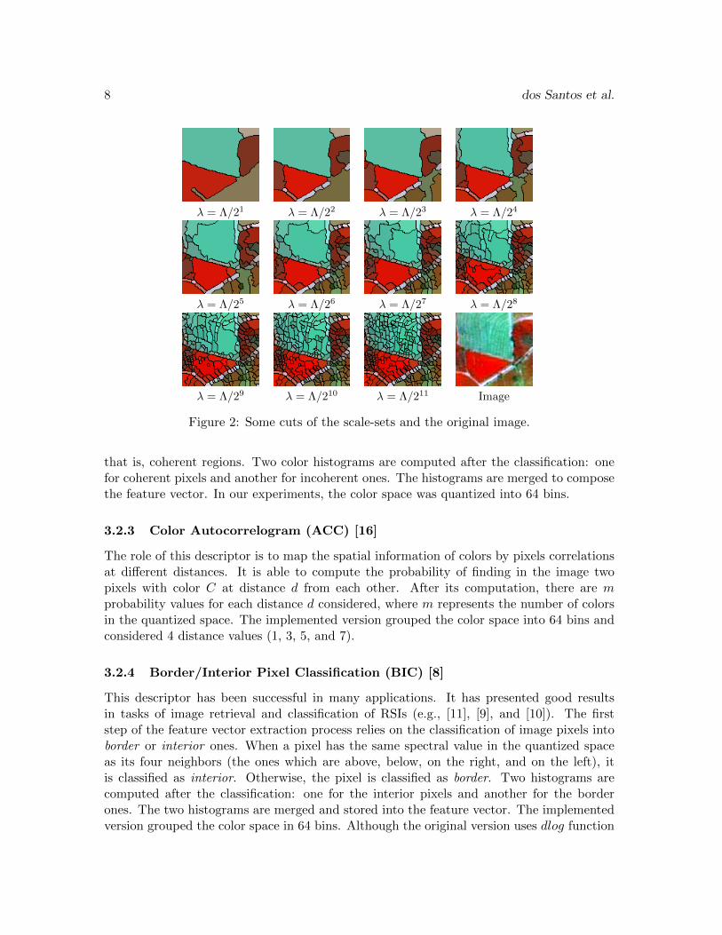
Let Λ be the maximum scale in the hierarchy H, i.e., the one in which the image I isrepresented by a single region, the cut-scale λ is defined by λ = Λ/2n, where n is the orderof each division in the hierarchy. Figure 2 presents some cuts extracted from the hierarchyillustrated in Figure 1.

The highest scale of the hierarchy shown in Figure 1 is Λ = 1.716. Thus, the first cut isdefined at the scale λ = 0.858, the second one at the scale λ = 0.429, and so on.

3.2 Image Descriptors

This paper uses the descriptor definition proposed in [7]. According to that work, a de-scriptor can be characterized by two functions: feature vector extraction and similaritycomputation. The feature vectors encode image properties, like color, texture, and shape.Therefore, the similarity between two images is computed as a function of their featurevector distance. Note that different types of feature vectors may require different similarityfunctions.

The multi-scale classification approach proposed is general with respect to the type offeatures used. In this article, we use seven descriptors from the literature: three texture de-scriptors and four descriptors that encode spectral features (color). In our implementation,all these descriptors use the L1 function to calculate distances between two feature vectors.We briefly present the function extraction of each descriptor below.


/2

/4

/8

/16

...

Figure 1: A scale-sets image representation. Horizontal axis: the regions. Vertical axis: thescales (logarithmic representation).

3.2.1 Global Color Histogram (GCH) [33]

Being one of the most commonly used descriptors, it uses an extraction algorithm whichquantizes the color space in a uniform way and it scans the image computing the number ofpixels belonged to each bin. The size of its feature vector is dependent on the quantizationused. In the present work, the color space was grouped into 64 bins, thus, the feature vectorhas 64 values.

3.2.2 Color Coherence Vector (CCV) [30]

This descriptor, like GCH, is recurrent in the literature. It uses an extraction algorithmthat classifies the image pixels as “coherent” or “incoherent” pixels. This classificationtakes into consideration whether the pixel belongs or not to a region with similar colors,

8 dos Santos et al.

λ = Λ/21 λ = Λ/22 λ = Λ/23 λ = Λ/24

λ = Λ/25 λ = Λ/26 λ = Λ/27 λ = Λ/28

λ = Λ/29 λ = Λ/210 λ = Λ/211 Image

Figure 2: Some cuts of the scale-sets and the original image.

that is, coherent regions. Two color histograms are computed after the classification: onefor coherent pixels and another for incoherent ones. The histograms are merged to composethe feature vector. In our experiments, the color space was quantized into 64 bins.

3.2.3 Color Autocorrelogram (ACC) [16]

The role of this descriptor is to map the spatial information of colors by pixels correlationsat different distances. It is able to compute the probability of finding in the image twopixels with color C at distance d from each other. After its computation, there are mprobability values for each distance d considered, where m represents the number of colorsin the quantized space. The implemented version grouped the color space into 64 bins andconsidered 4 distance values (1, 3, 5, and 7).

3.2.4 Border/Interior Pixel Classification (BIC) [8]

This descriptor has been successful in many applications. It has presented good resultsin tasks of image retrieval and classification of RSIs (e.g., [11], [9], and [10]). The firststep of the feature vector extraction process relies on the classification of image pixels intoborder or interior ones. When a pixel has the same spectral value in the quantized spaceas its four neighbors (the ones which are above, below, on the right, and on the left), itis classified as interior. Otherwise, the pixel is classified as border. Two histograms arecomputed after the classification: one for the interior pixels and another for the borderones. The two histograms are merged and stored into the feature vector. The implementedversion grouped the color space in 64 bins. Although the original version uses dlog function


distance, the used version was adapted to use L1 distances.

3.2.5 Invariant Steerable Pyramid Decomposition (SID) [43]

In this descriptor, a set of filters sensitive to different scales and orientations processesthe image. The image is first decomposed into two sub-bands by a high-pass filter anda low-pass one. After that, the low-pass sub-band is decomposed recursively into K sub-bands by band-pass filters and into one sub-band by a low-pass filter. Different directionalinformation about each scale is captured by each recursive step. The mean and standarddeviation of each sub-band are used as feature vector values. To obtain the invariance toscale and orientation, circular shifts in the feature vector are applied. The implementedversion uses 2 scales and 4 orientations, which results in a feature vector with 16 values.

3.2.6 Unser [38]

This descriptor is based on co-occurrence matrices, still one of the most widely used descrip-tors to encode texture in remote sensing applications. Its extraction algorithm computesa histogram of sums Hsum and a histogram of differences Hdif . The histogram of sums isincremented considering the sum, while the histogram of differences is incremented takinginto account the difference between the values of two neighbor pixels. Like gray level co-occurrence matrices, measures such as energy, contrast, and entropy can be extracted fromthe histograms. In our experiments, 256 gray levels and 4 angles were used (0◦, 45◦, 90◦,and 135◦). The feature vector is composed of 32 values and eight different measures wereextracted from histograms.

3.2.7 Quantized Compound Change Histogram (QCCH) [15]

It uses the relation between pixels and their neighbors to encode texture information. Thisdescriptor generates a representation invariant to rotation and translation. Its extractionalgorithm scans the image with a square window. For each position in the image, theaverage gray value of the window is computed. Next, four variation rates are computed bytaking into consideration the average gray values and the horizontal, vertical, diagonal, andanti-diagonal directions. The average of these four variations is calculated for each windowposition, they are grouped into 40 bins and a histogram of these values is computed.

4 Multi-Scale Training and Classification

In the following sections, we describe the ideas on which the proposed approaches rely, aswell as the major processing steps for multi-scale classification. In Section 4.1, we introducethe concepts and the general functioning of the proposed approach. In Section 4.2 and 4.3,the two approaches that we propose for training classifiers using multi-scales are presented.Finally, in Section 4.4 we describe the weak classifiers used in this paper.

10 dos Santos et al.

4.1 Classification Principles

The aim of RSI classification is to build a classification function F (p) that returns a clas-sification score (+1 for relevant, and −1 otherwise) for each pixel p of an RSI. Let us notethat, even if the classification returns a result at a pixel level, the decision may be based onregions of different scales containing the pixel.

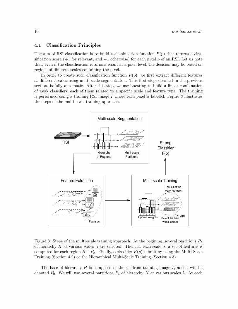
In order to create such classification function F (p), we first extract different featuresat different scales using multi-scale segmentation. This first step, detailed in the previoussection, is fully automatic. After this step, we use boosting to build a linear combinationof weak classifiers, each of them related to a specific scale and feature type. The trainingis performed using a training RSI image I where each pixel is labeled. Figure 3 illustratesthe steps of the multi-scale training approach.

RSI

Multi-scale Segmentation

Hierarchyof Regions

Multi-scalePartitions

Feature Extraction

Features

Multi-scale Training

Update Weights

Test all of theweak learners

h (p)t Select the bestweak learner

StrongClassifier

F(p)

Figure 3: Steps of the multi-scale training approach. At the begining, several partitions Pλof hierarchy H at various scales λ are selected. Then, at each scale λ, a set of features iscomputed for each region R ∈ Pλ. Finally, a classifier F (p) is built by using the Multi-ScaleTraining (Section 4.2) or the Hierarchical Multi-Scale Training (Section 4.3).

The base of hierarchy H is composed of the set from training image I, and it will bedenoted P0. We will use several partitions Pλ of hierarchy H at various scales λ. At each


scale λ, a set of features is computed for each region of Pλ. These features can be differentaccording to the level, and, thus, to the size of the regions. For example, a texture featureis not appropriate for too small regions and a histogram (such as color histogram) is lessaccurate for large regions.

4.2 Multi-Scale Training

The multi-scale classifier (MSC) aims to assign a label (+1 for relevant class, and −1otherwise) to each pixel of P0 taking advantage of various features computed on regionsof various levels of the hierarchy. To build multi-scale classifiers, we propose a learningstrategy based on boosting of weak learners. This strategy is based on AdaBoost algorithmproposed by Schapire [31], which builds a linear combination MSC(p) of T weak classifiersht(p):

MSC(p) = sign( T∑t=1

αtht(p))

(1)

The proposed algorithm repeatedly calls weak learners in a series of rounds t = 1, . . . T .Each weak learner creates a weak classifier that decreases the expected classification errorof the combination. The algorithm then selects the weak classifier that most decreases theerror.

The strategy consists in keeping a set of weights over the training set. These weightscan be interpreted as a measure of the difficulty level to classify each training sample. Atthe beginning, all the pixels have the same weight, but in each round, the weights of themisclassified pixels are increased. Thus, in the next rounds the weak learners are forced tofocus on harder samples. We will note Wt(p) the weight of pixel p in round t, and Dt,λ(R)the misclassification rate of region R in round t at scale λ given by the mean of the weightsof its pixels:

Dt,λ(R) =( 1

|R|∑p∈R

Wt(p))

(2)

Algorithm 1 presents the proposed Multi-Scale Training process. Let Yλ(R), the set oflabels of regions R at scale λ, be the training set. In a serie of rounds t = 1, . . . T , for allscales λ, the weight of each region Dt,λ(R) is computed (line 3). This piece of informationis used to select the regions to be used for training the weak learners, building a subset oflabeled regions Yt,λ (line 6). The subset Yt,λ is used to train the weak learners with eachfeatures F at scale λ (line 9). Each weak learner produces a weak classifier ht,(F ,λ) (line10). The algorithm then selects the weak classifier ht that most decreases the error Errht(line 12). The level of error of ht is used to compute the coefficient αt, which indicates thedegree of importance of ht in the final classifier (line 13). The selected weak classifier htand the coefficient αt are used to update the weights of the pixels W(t+1)(p) which can beused in the next round (line 14).

The classification error of the classifier h is:


Algorithm 1 Multi-Scale Training

Given:Training labels Yλ(R) = labels of regions R at scale λ

Initialize:For all pixels p, W1(p)← 1

|Y0|, where |Y0| is the number of pixels in the image level

1 For t← 1 to T do2 For all scales λ do3 For all R ∈ Pλ do4 Compute Dt,λ(R)5 End for

6 Build Yt,λ (a training subset based on Dt,λ(R))7 End for8 For each pair feature/scale (F , λ) do

9 Train weak learners using features (F , λ) and training set Yt,λ.10 Evaluate resulting classifier ht,(F ,λ): compute Err(ht,(F ,λ),W )) (Equation 3)

11 End for12 Select weak classifier ht = argminht,(F,λ) Err(ht,(F ,λ),Wt,λ)

13 Compute αt ← 12 ln(1+rt1−rt

)with rt ←

∑p cY0(p)ht(p)

14 Update Wt+1(p)←Wt(p) exp (−αtY0(p)ht(p))∑p

Wt(p) exp (−αtY0(p)ht(p))

15 End for

Output: Multi-Scale Classifier MSC(p)

Err(h,W ) =∑

p|h(p)Y0(p)<0

W (p) (3)

The training is performed on the training set labels Yλ corresponding to the same scale λ.The weak learners (linear SVM, for example) use the subset Yt,λ for training and producea weak classifier ht,(F ,λ). The training set labels Y0 are the labels of pixels of image I,and training sets labels Yλ with λ > 0 are defined according to the proportions of pixelsbelonging to one of the two classes (for example, at least 80% of one region).

The idea of building the subs Y is to force the classifiers to train with the most difficultsamples. The weak learner should allow the most difficult samples to be differentiatedfrom the other ones according to their weight. Thus, the strategy of creating Y is directlydependent on the configuration of the weak classifier and may contain all regions, since theclassifier considers the weights of the samples.


4.3 Hierarchical Training

The Multi-Scale Training presented in Section 4.2 creates a classifier based on linear com-bination of weak classifiers. In this case, both the selection of scales and features, and theweights of each weak classifier are obtained by a strategy based on AdaBoost. Althoughthis approach provides the selection of the most appropriate scales to the training set, itdoes not ensure the representation of all scales in the final result. In addition, the cost oftraining with each scale is proportional to the number of regions it contains. However, thecoarse scales are not always selected, which means that training time can be reduced if weavoid this analysis.

As an attempt to overcome these problems, we propose a hierarchical multi-scale classi-fication scheme. The proposed strategy is presented in Figure 4. It consists of individuallyselecting the weak classifiers for each scale, starting from coarser to finer ones. Thereby,each scale provides a different stage of training. At the end of each stage, only the mostdifficult samples are selected, limiting the training set used in the next stage. In each stage,the process is similar to that one described in Algorithm 1. However, the weak learners aretrained with only the features related to the current scale. For each scale, the weak learnerproduces a set Hλ of weak classifiers.

k

AdaboostTrainingImage

hardsamples

easy samples

k-1

Adaboosthard

samples

easy samples

t=1

T

t th (p)

t=1

T

t th (p)

scale k scale k-1

2

Adaboosthard

samples

easy samples

1

Adaboost

t=1

T

t th (p)

t=1

T

t th (p)

scale 2 scale 1

...

...

F1 Fn...F1 Fn... F1 Fn...

F1 Fn...

Figure 4: The hierarchical multi-scale training strategy.

The hierarchical multi-scale classifier (HMSC) is a combination of the set of weakclassifiers Sλ(p) selected for each scale λ:

HMSC(p) = sign(∑

λi

Sλi(p))

= sign(∑

λi

T∑t=1

αt,λiht,λi(p))

(4)

where T is the number of rounds for each boosting step.

At the end of each stage, we withdraw the easiest samples. Let Wi be the weights of thepixels after training with scale λi, we denote Di(Ri+1) the weight of the region Ri+1 ∈ Pλi+1

,


which is given by:

Di(Ri+1) =( 1

|R|∑p∈R

Wi(p))

(5)

The set of regions Yi+1 to be used in the training stage with scale λi+1 is composed

by the regions Ri+1 ∈ Pλi+1with mean Di(Ri+1) >

12|Y0|

. This means that the regions

that ended a training stage with distribution equal to half the initialization value 1|Y0|

, are

discarded from one stage to another.

4.4 Weak Classifiers

In this paper, we adopted two configurations of weak learners: Suport Vector Machines(SVM) and Radial Basis Function (RBF). The RBF approach is based on the distancesprovided by the used descriptors.

4.4.1 SVM-based weak learner

It is an SVM trainer based on a specific feature type F and a specific scale λ. Given thetraining subset labels Yλ, the strategy is to find the best linear hyperplane of separationbetween RSI regions according to their classes (coffee and non-coffee regions), trying tomaximize the data separation margin. These samples are called support vectors and arefound during the training. Once the support vectors and the decision coeffients (αi, i =1, . . . , N) are found, the SVM weak classifier can be defined as:

SVM(F ,λ)(R) = sign( N∑

i

yiαi(fR · fi) + b)

(6)

where b is a parameter found during the training. The support vectors are the fi such thatα > 0, yi is the support vector class and fR is the feature vector of the region.

The training subset Yt,λ is composed by n labels from Yλ with values of Dt,λ(R) bigger

or equal to 1|Y0|

. This strategy means that only regions considered as the most difficult

ones are used for the training. For the first round of boosting, the regions to compose thesubset Y0,λ are randomly selected.

The weakness of the linear SVM classifier is due to our strategy of creating subsetsinstead of providing all regions of a partition for training. It decreases the power of theproduced classifier. Moreover, in our experiments the dimension of the feature space issmaller than the number of samples, which theoretically guarantees the weakness of linearclassifiers.

4.4.2 RBF-based weak learner

It consists of selecting a target region that best separates the other regions between bothclasses based on a specific image descriptor D and a specific scale λ. The distances are


normalized with the sigmoid function.

The RBF-based weak learner tests all training regions (i.e, Yλ = Yλ) as targets in theclassification task. The exception are the regions that have already been used as targets.

Let Rt be a target region and y its class. The class of region R, given by the weakclassifier (Rt, D, λ), is defined by:

RBF(Rt,D,λ)(R) =

{y, if d(Rt, R) ≤ l−y, otherwise

(7)

where d(Rt, R) is the distance between the target region Rt and region R using descriptorD and l is a threshold value.

5 Experiments

In this section, we present the experiments that we performed to validate our method. Wehave carried out experiments in order to address the following research questions:

• Is the set of used descriptors effective for object-based RSI classification task (Sec-tion 5.2.1)?

• Is the multi-scale classification results effective in RSI tasks (Section 5.2.2)?

• Are the proposed weak learners effective in the RSI classification problem (Section 5.2.3)?

• Can the hierarchical strategy for multi-scale improve the classification results (Sec-tion 5.2.4)?

• Are the proposed methods effective in the RSI classification problem when comparedto a baseline (Section 5.2.5)?

In Section 5.1, we describe the basic configuration of our experiments. In Section 5.2we present the experimental results.

5.1 Setup

5.1.1 Dataset

The dataset used in our experiments is a composition of scenes taken by the SPOT sensor in2005 over Monte Santo de Minas county, in the State of Minas Gerais, Brazil. This area is atraditional place of coffee cultivation, characterized by its mountainous terrain. In additionto common issues in the area of pattern recognition in remote sensing images, these factorsadd further problems that must be taken into account. In mountainous areas, the spectralpatterns tend to be affected by the topographical differences and interference generated bythe shadows. This dataset provides an ideal environment for multi-scale analysis, since thevariations in topography require the cultivation of coffee in different crop sizes. Anotherproblem is that coffee is not an annual crop. This means that, in the same area, there may


be plantations of different ages, as illustrated in Figure 5. In terms of classification, wehave several completely different patterns representing the same class while some of thesepatterns are much closer to other classes.

97 1

2

3

4

5

6

7

8

9

10

Coffee Non-coffee9

1

10

4

2

3

5

6

8

Figure 5: Example of coffee and non-coffee samples in the used RSI. Note the differenceamong the samples of coffee and their similarities with non-coffee samples [9].

We have used a complete mapping of the coffee areas in the dataset for training andassessing the quality of experimental results. The identification of coffee crops was donemanually in the whole county by agricultural researchers. They used the original image asreference and visited the place to compose the final result.

The dimensions of the image used are 3000× 3000 pixels with spatial resolution equalsto 2.5 meters. To facilitate the experimental protocol, we divided the dataset into a gridof 3 × 3, generating 9 subimages with dimensions equal to 1000 × 1000 pixels. In theexperiments, we used 9 different sets with size equals to 1 million pixels each, to be usedfor training and testing. In the experiments we have used 5 of these sets. The results of theexperiments described in the following sections are obtained from all combinations of the 5subimages used, training with 3 of them and testing with 2 subimages.

5.1.2 Feature Extraction

Unlike conventional images, RSI bands do not usually correspond exactly to the humanvisible spectrum. To apply conventional image descriptors (which generally use three colorchannels), it is necessary to select the most informative bands. Therefore, we used only thebands corresponding to “red”, “infrared”, and “green” that are fundamental to describevegetation targets. These spectral bands are the basis for most of the vegetation indexes [24].

We extracted seven different features from the band composition IR-NIR-R (342) byusing 4 color descriptors (ACC [16], BIC [8], CCV [30], and GCH [33]) and 3 texturedescriptors (Unser [38], SID [43], and QCCH [15]). These descriptors were presented inSection 3.2.


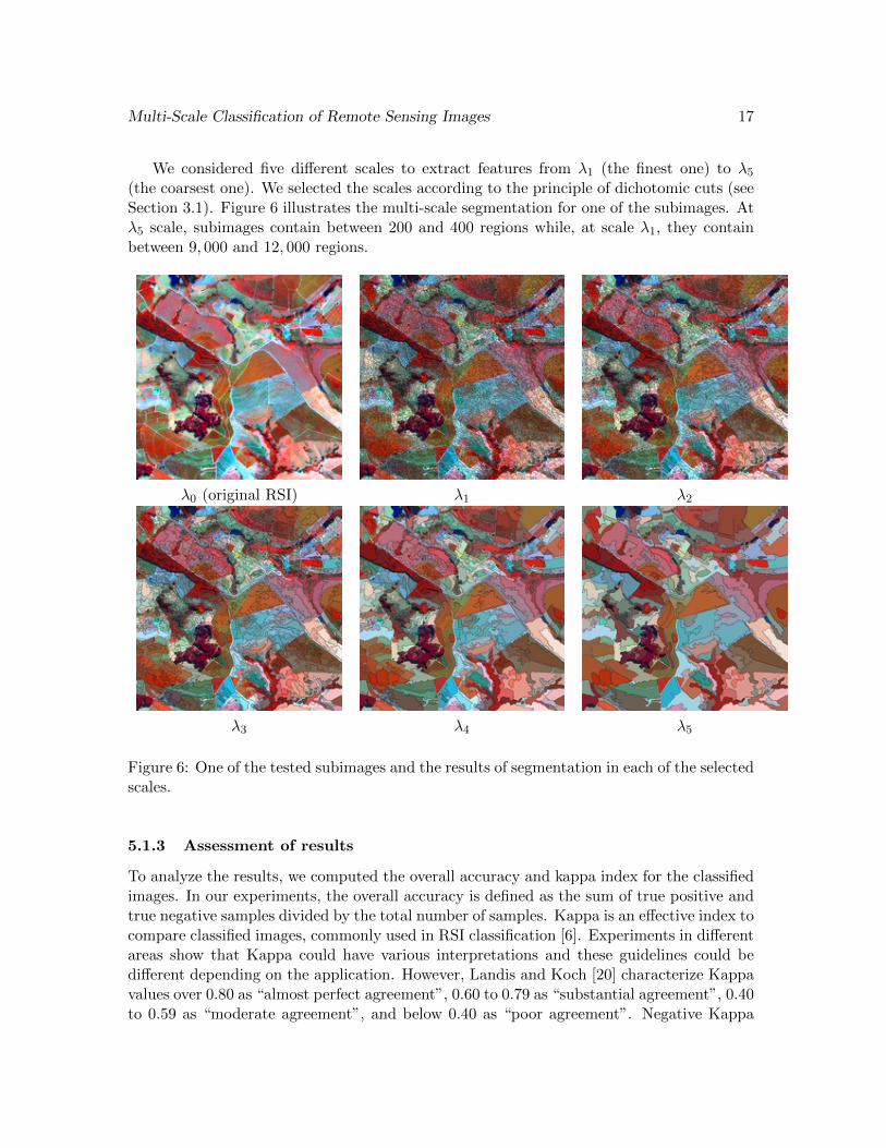
We considered five different scales to extract features from λ1 (the finest one) to λ5(the coarsest one). We selected the scales according to the principle of dichotomic cuts (seeSection 3.1). Figure 6 illustrates the multi-scale segmentation for one of the subimages. Atλ5 scale, subimages contain between 200 and 400 regions while, at scale λ1, they containbetween 9, 000 and 12, 000 regions.

λ0 (original RSI) λ1 λ2

λ3 λ4 λ5

Figure 6: One of the tested subimages and the results of segmentation in each of the selectedscales.

5.1.3 Assessment of results

To analyze the results, we computed the overall accuracy and kappa index for the classifiedimages. In our experiments, the overall accuracy is defined as the sum of true positive andtrue negative samples divided by the total number of samples. Kappa is an effective index tocompare classified images, commonly used in RSI classification [6]. Experiments in differentareas show that Kappa could have various interpretations and these guidelines could bedifferent depending on the application. However, Landis and Koch [20] characterize Kappavalues over 0.80 as “almost perfect agreement”, 0.60 to 0.79 as “substantial agreement”, 0.40to 0.59 as “moderate agreement”, and below 0.40 as “poor agreement”. Negative Kappa


means that there is no agreement between classified data and verification data.

5.2 Results

5.2.1 Descriptors Comparison

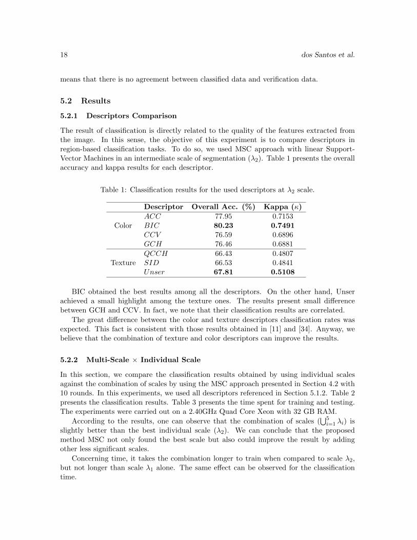
The result of classification is directly related to the quality of the features extracted fromthe image. In this sense, the objective of this experiment is to compare descriptors inregion-based classification tasks. To do so, we used MSC approach with linear Support-Vector Machines in an intermediate scale of segmentation (λ2). Table 1 presents the overallaccuracy and kappa results for each descriptor.

Table 1: Classification results for the used descriptors at λ2 scale.

Descriptor Overall Acc. (%) Kappa (κ)

ColorACC 77.95 0.7153BIC 80.23 0.7491CCV 76.59 0.6896GCH 76.46 0.6881

TextureQCCH 66.43 0.4807SID 66.53 0.4841Unser 67.81 0.5108

BIC obtained the best results among all the descriptors. On the other hand, Unserachieved a small highlight among the texture ones. The results present small differencebetween GCH and CCV. In fact, we note that their classification results are correlated.

The great difference between the color and texture descriptors classification rates wasexpected. This fact is consistent with those results obtained in [11] and [34]. Anyway, webelieve that the combination of texture and color descriptors can improve the results.

5.2.2 Multi-Scale × Individual Scale

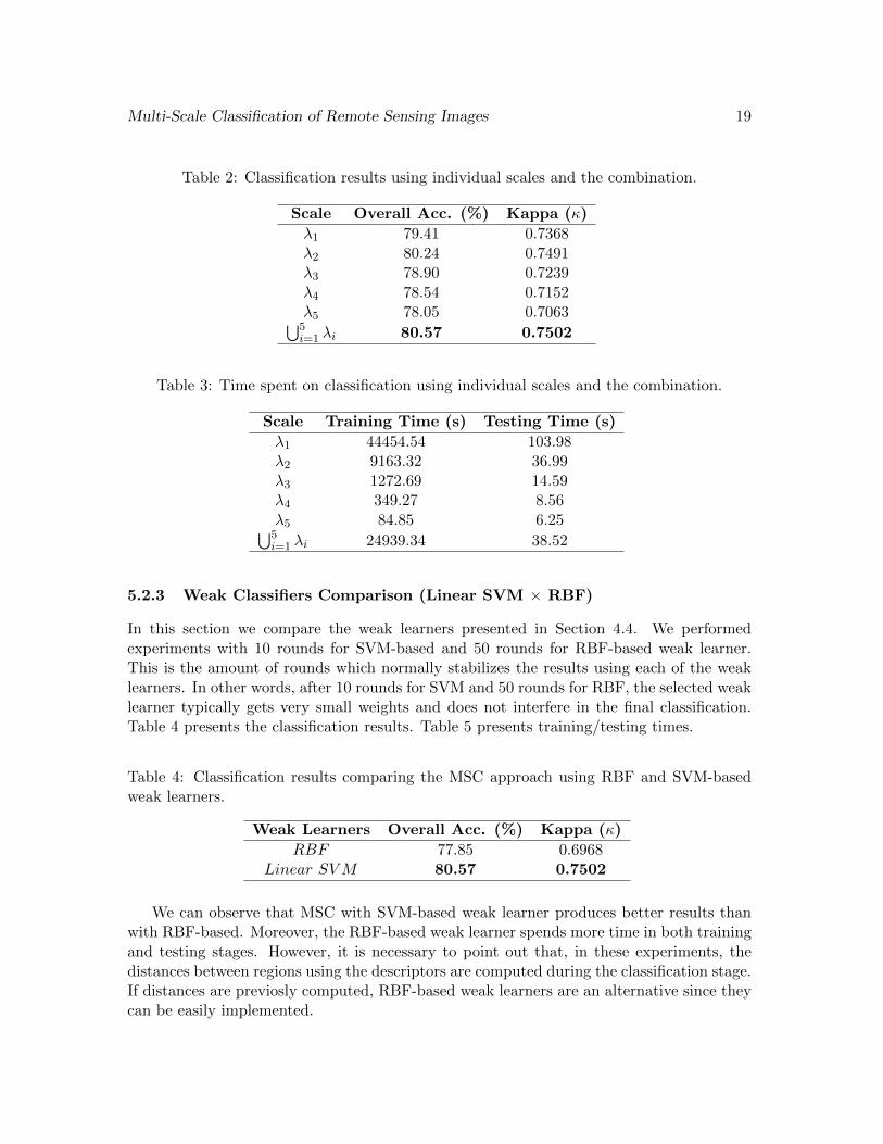
In this section, we compare the classification results obtained by using individual scalesagainst the combination of scales by using the MSC approach presented in Section 4.2 with10 rounds. In this experiments, we used all descriptors referenced in Section 5.1.2. Table 2presents the classification results. Table 3 presents the time spent for training and testing.The experiments were carried out on a 2.40GHz Quad Core Xeon with 32 GB RAM.

According to the results, one can observe that the combination of scales (⋃5i=1 λi) is

slightly better than the best individual scale (λ2). We can conclude that the proposedmethod MSC not only found the best scale but also could improve the result by addingother less significant scales.

Concerning time, it takes the combination longer to train when compared to scale λ2,but not longer than scale λ1 alone. The same effect can be observed for the classificationtime.


Table 2: Classification results using individual scales and the combination.

Scale Overall Acc. (%) Kappa (κ)

λ1 79.41 0.7368λ2 80.24 0.7491λ3 78.90 0.7239λ4 78.54 0.7152λ5 78.05 0.7063⋃5i=1 λi 80.57 0.7502

Table 3: Time spent on classification using individual scales and the combination.

Scale Training Time (s) Testing Time (s)

λ1 44454.54 103.98λ2 9163.32 36.99λ3 1272.69 14.59λ4 349.27 8.56λ5 84.85 6.25⋃5i=1 λi 24939.34 38.52

5.2.3 Weak Classifiers Comparison (Linear SVM × RBF)

In this section we compare the weak learners presented in Section 4.4. We performedexperiments with 10 rounds for SVM-based and 50 rounds for RBF-based weak learner.This is the amount of rounds which normally stabilizes the results using each of the weaklearners. In other words, after 10 rounds for SVM and 50 rounds for RBF, the selected weaklearner typically gets very small weights and does not interfere in the final classification.Table 4 presents the classification results. Table 5 presents training/testing times.

Table 4: Classification results comparing the MSC approach using RBF and SVM-basedweak learners.

Weak Learners Overall Acc. (%) Kappa (κ)

RBF 77.85 0.6968Linear SVM 80.57 0.7502

We can observe that MSC with SVM-based weak learner produces better results thanwith RBF-based. Moreover, the RBF-based weak learner spends more time in both trainingand testing stages. However, it is necessary to point out that, in these experiments, thedistances between regions using the descriptors are computed during the classification stage.If distances are previosly computed, RBF-based weak learners are an alternative since theycan be easily implemented.


Table 5: Time spent on classification using the MSC approach with RBF and SVM-basedweak learners.

Weak Learners Training Time (s) Testing Time (s)

RBF 31030.987 327.01Linear SVM 24939.34 38.52

5.2.4 Hierarchical MS-Classification

In this section we present the results of the proposed Hierarchical Multi-Scale Classificationapproach. Table 6 presents the overall accuracy and Kappa index for HMSC against MSCapproach. Time is presented in Table 7. We used 10 rounds for MSC and 50 rounds forHMSC (10 rounds for each scale). To maintain the detection time of the classifier HMSCequivalent to the MSC, the weak learners with very low weights are excluded from thefinal classifier: the threshold on the weights is 0.01. This reduces the final classifier to acombination between 10 and 15 weak learners.

Table 6: Classification results comparing the HMSC against MSC.

Method Overall Acc. (%) Kappa (κ)

HMSC 82.09 0.7772MSC 80.57 0.7502

Table 7: Time spent on classification for MSC and HMSC.

Method Training Time (s) Testing Time (s)

HMSC 13637.62 39.06MSC 24939.34 38.52

As it can be seen, the hierarchical approach improves the classification results. There-fore, we conclude that by forcing the combination of scales improved results can be yielded.Actually, the key difference between the approaches is that MSC selects only weak learnersthat are expected to be the best ones, which may exclude some scales of the final result.The HMSC, on the contrary, selects weak learners at all scales. Even if the weights ofthese scales is small, it seems to affect positively the final result of classification.

Another important point concerns the training time. As the hierarchical approach doesnot use all regions of all scales, training time is considerably reduced because the trainingfocuses only on the most difficult regions.

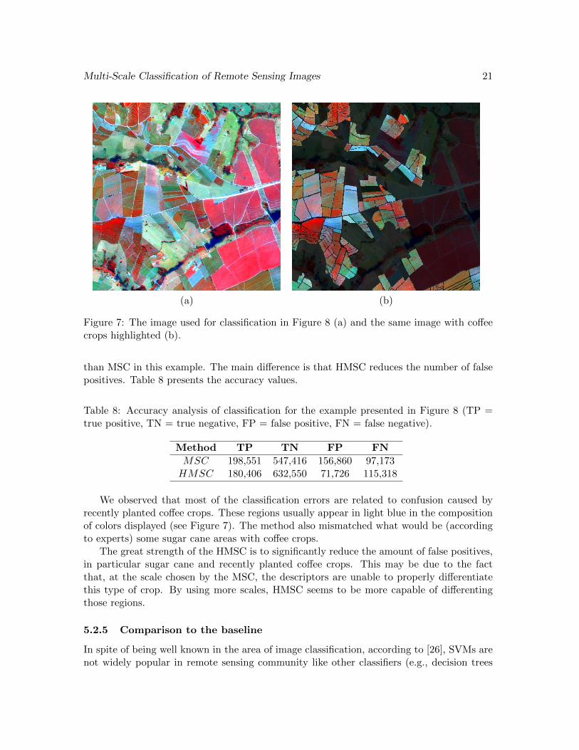
Figure 7 (a) shows a subimage used in experiments and Figure 7 (b) illustrates the sameimage with coffee crops, which are the regions of interest in focus. Figures 8 (a) and (b)illustrate an example of result obtained with the methods HMSC and MSC, respectively.

As one can see when comparing Figures 8 (a) and 8 (b), HMSC produces better results


(a) (b)

Figure 7: The image used for classification in Figure 8 (a) and the same image with coffeecrops highlighted (b).

than MSC in this example. The main difference is that HMSC reduces the number of falsepositives. Table 8 presents the accuracy values.

Table 8: Accuracy analysis of classification for the example presented in Figure 8 (TP =true positive, TN = true negative, FP = false positive, FN = false negative).

Method TP TN FP FN

MSC 198,551 547,416 156,860 97,173HMSC 180,406 632,550 71,726 115,318

We observed that most of the classification errors are related to confusion caused byrecently planted coffee crops. These regions usually appear in light blue in the compositionof colors displayed (see Figure 7). The method also mismatched what would be (accordingto experts) some sugar cane areas with coffee crops.

The great strength of the HMSC is to significantly reduce the amount of false positives,in particular sugar cane and recently planted coffee crops. This may be due to the factthat, at the scale chosen by the MSC, the descriptors are unable to properly differentiatethis type of crop. By using more scales, HMSC seems to be more capable of differentingthose regions.

5.2.5 Comparison to the baseline

In spite of being well known in the area of image classification, according to [26], SVMs arenot widely popular in remote sensing community like other classifiers (e.g., decision trees


(a) (b)

Figure 8: A result obtained with the proposed methods: MSC (a) and HMSC (b). Pixelscorrectly classified are shown in white (true positive) and black (true negative) while theerrors are displayed in red (false positive) and green (false negative).

and variants of neural networks). Meanwhile, in recent years there has been a significantincrease in SVM works achieving very good results in remote sensing problems. Tzotsos etal. [35] have proposed and evaluated SVMs for object-oriented classification. They proposedan approach that uses SVMs with RBF kernels to classify the regions obtained from a multi-scale segmentation process. That approach outperforms the results obtained by using thesoftware eCognition [1]. Therefore, we used SVM + RBF kernels applied to an intermediatesegmentation scale obtained by Guigues method as baseline with BIC descriptor. Table 9presents the results.

Table 9: Classification results comparing the MSC, HMSC and the baseline.

Method Overall Acc. (%) Kappa (κ)

SVM +RBF 77.47 0.7054MSC (SVM learner) 80.57 0.7502HMSC (SVM learner) 82.09 0.7772

As it can be noticed, both the MSC and HMSC overcome the results of the adoptedbaseline. This shows that the combination of descriptors and scales using the strategiesproposed in this work can be powerful tools for classification of remote sensing images.


6 Conclusions

We have shown in this paper that: region-based classification is a good alternative to pixelclassification; the descriptors computed on regions are more reliable than those computedon pixels or on regular blocks; the most relevant regions in different parts and scales of theimage and features at various scales can be learned during the design of the classificationmachine.

The proposed approaches for multiscale image analysis are: the Multi-Scale Classifier(MSC) and the Hierarchical Multi-Scale Classifier (HMSC). The MSC is a boosting-basedclassifier that builds a strong classifier from a set of weak ones. The HMSC is also basedon boosting of weak classifiers, but it adopts a sequential strategy of training, according tothe segmentation hierarchy of scales (from coarser to finner). In this work, we adopted twoconfigurations of weak learners: SVM and RBF. The SVM approach is based on the SVMclassifier with linear kernel. The other one is based on the distances provided by RadialBasis Function and the used descriptors.

The experimental results shows that the BIC descriptor is presently the most powerfuldescriptor to detect regions of coffee. The MSC method chooses the scales more appropriateto the training set. HMSC reduces training time when compared to MSC. In experiments,HMSC also improves the classification results. This suggests that forcing the combinationof scales may increase the power of the final classifier.

Our perspectives are firstly to build a very fast classifier by using a cascade of classifiersand secondly to improve the learning set through user interaction.

Acknowledgments

The authors are grateful to CAPES, FAPESP, and CNPq for the financial support. We aregrateful to Jean Pierre Cocquerez for the support concerning the segmentation tool. Wealso thank Rubens Lamparelli due to the support related to agricultural aspects and theremote sensing dataset.

References

[1] Ursula C. Benz, Peter Hofmann, Gregor Willhauck, Iris Lingenfelder, and MarkusHeynen. Multi-resolution, object-oriented fuzzy analysis of remote sensing data forgis-ready information. ISPRS Journal of Photogrammetry and Remote Sensing, 58(3-4):239 – 258, 2004. Integration of Geodata and Imagery for Automated Refinementand Update of Spatial Databases.

[2] T. Blaschke. Object based image analysis for remote sensing. ISPRS Journal ofPhotogrammetry and Remote Sensing, 65(1):2 – 16, 2010.

[3] Castillejo-Gonzalez, Lopez-Granados, Garcıa-Ferrer, Pena-Barragan, Jurado-Exposito,de la Orden, and Gonzalez-Audicana. Object- and pixel-based analysis for mapping


crops and their agro-environmental associated measures using quickbird imagery. Com-puters and Electronics in Agriculture, 68(2):207 – 215, 2009.

[4] Jianyu Chen, Delu Pan, and Zhihua Mao. Imageobject detectable in multiscale analysison highresolution remotely sensed imagery. International Journal of Remote Sensing,30(14):3585–3602, 2009.

[5] Yunhao Chen, Wei Su, Jing Li, and Zhongping Sun. Hierarchical object oriented clas-sification using very high resolution imagery and lidar data over urban areas. Advancesin Space Research, 43(7):1101 – 1110, 2009.

[6] Russel G. Congalton and Kass Green. Assessing the Accuracy of Remotely SensedData: Principles and Practices. Lewis Publishersr, Washington, DC, 1977.

[7] R. da S. Torres and A. X. Falcao. Content-Based Image Retrieval: Theory and Appli-cations. Revista de Informatica Teorica e Aplicada, 13(2):161–185, 2006.

[8] R. de O. Stehling, M. A. Nascimento, and A. X. Falcao. A compact and efficientimage retrieval approach based on border/interior pixel classification. In CIKM, pages102–109, New York, NY, USA, 2002.

[9] J. A. dos Santos, F. A. Faria, R. T. Calumby, R. da S. Torres, and R. A. C. Lamparelli.A genetic programming approach for coffee crop recognition. In IGARSS 2010, pages3418–3421, Honolulu, USA, July 2010.

[10] J. A. dos Santos, C. D. Ferreira, R. da S.Torres, M. A. Goncalves, and R. A. C. Lam-parelli. A relevance feedback method based on genetic programming for classificationof remote sensing images. Information Sciences, 181(13):2671 – 2684, 2011.

[11] J. A. dos Santos, O. A. B. Penatti, and R. da S. Torres. Evaluating the potential oftexture and color descriptors for remote sensing image retrieval and classification. InVISAPP 2010, pages 203–208, Angers, France, May 2010.

[12] R. Gaetano, G. Scarpa, and G. Poggi. Hierarchical texture-based segmentation ofmultiresolution remote-sensing images. Geoscience and Remote Sensing, IEEE Trans-actions on, 47(7):2129 –2141, july 2009.

[13] X. Gigandet, M.B. Cuadra, A. Pointet, L. Cammoun, R. Caloz, and J.-Ph. Thiran.Region-based satellite image classification: method and validation. ICIP 2005., 3:III–832–5, September 2005.

[14] L. Guigues, J. Cocquerez, and H. Le Men. Scale-sets image analysis. InternationalJournal of Computer Vision, 68:289–317, 2006.

[15] C. Huang and Q. Liu. An orientation independent texture descriptor for image retrieval.International Conference on Communications, Circuits and Systems, pages 772–776,July 2007.


[16] J. Huang, S. R. Kumar, M. Mitra, W. Zhu, and R. Zabih. Image indexing using colorcorrelograms. In Proceedings of the 1997 Conference on Computer Vision and PatternRecognition, page 762, Washington, DC, USA, 1997.

[17] Wen jie Wang, Zhong ming Zhao, and Hai qing Zhu. Object-oriented change detectionmethod based on multi-scale and multi-feature fusion. In Urban Remote Sensing Event,2009 Joint, pages 1 –5, may 2009.

[18] A. Katartzis, I. Vanhamel, and H. Sahli. A hierarchical markovian model for multiscaleregion-based classification of vector-valued images. IEEE Transactions on Geoscienceand Remote Sensing, 43(3):548–558, March 2005.

[19] Minho Kim, Timothy A. Warner, Marguerite Madden, and Douglas S. Atkinson. Multi-scale geobia with very high spatial resolution digital aerial imagery: scale, texture andimage objects. International Journal of Remote Sensing, 32(10):2825–2850, 2011.

[20] J. R. Landis and G. G. Koch. The measurement of observer agreement for categoricaldata. Biometrics, 33(1):159–174, March 1977.

[21] J.Y. Lee and T. A. Warner. Image classification with a region based approach in highspatial resolution imagery. In Int. Archives of Photogrammetry, Remote Sensing andSpatial Inf. Sciences, pages 181–187, Istanbul, Turkey, July 2004.

[22] Haitao Li, Haiyan Gu, Yanshun Han, and Jinghui Yang. An efficient multiscale srmmhr(statistical region merging and minimum heterogeneity rule) segmentation method forhigh-resolution remote sensing imagery. Selected Topics in Applied Earth Observationsand Remote Sensing, IEEE Journal of, 2(2):67 –73, june 2009.

[23] N. Li, H. Huo, and T. Fang. A novel texture-preceded segmentation algorithm for high-resolution imagery. Geoscience and Remote Sensing, IEEE Transactions on, (99):1 –11,2010.

[24] T. M. Lillesand, R. W. Kiefer, and Jonathan W. Chipman. Remote Sensing and ImageInterpretation. Wiley, 2007.

[25] D. Lu and Q. Weng. A survey of image classification methods and techniques forimproving classification performance. Int. J. Remote Sens., 28(5):823–870, 2007.

[26] Giorgos Mountrakis, Jungho Im, and Caesar Ogole. Support vector machines in remotesensing: A review. ISPRS Journal of Photogrammetry and Remote Sensing, 66(3):247– 259, 2011.

[27] D. Mumford and J. Shah. Optimal approximations by piecewise smooth functions andassociated variational problems. Communications on Pure and Applied Mathematics,42(5):577–685, 1989.

[28] Soe W. Myint, Patricia Gober, Anthony Brazel, Susanne Grossman-Clarke, and QihaoWeng. Per-pixel vs. object-based classification of urban land cover extraction using


high spatial resolution imagery. Remote Sensing of Environment, 115(5):1145 – 1161,2011.

[29] Yashon O. Ouma, S.S. Josaphat, and Ryutaro Tateishi. Multiscale remote sensingdata segmentation and post-segmentation change detection based on logical modeling:Theoretical exposition and experimental results for forestland cover change analysis.Computers and Geosciences, 34(7):715 – 737, 2008.

[30] G. Pass, R. Zabih, and J. Miller. Comparing images using color coherence vectors. InACM Multimedia, pages 65–73, 1996.

[31] Robert E. Schapire. A brief introduction to boosting. In Proceedings of the SixteenthInternational Joint Conference on Artificial Intelligence, IJCAI ’99, pages 1401–1406,1999.

[32] R. Showengerdt. Techniques for Image Processing and Classification in Remote Sens-ing. Academic Press, New York, 1983.

[33] M. J. Swain and D. H. Ballard. Color indexing. International Journal of ComputerVision, 7(1):11–32, 1991.

[34] Roger Trias-Sanz, Georges Stamon, and Jean Louchet. Using colour, texture, andhierarchial segmentation for high-resolution remote sensing. ISPRS Journal of Pho-togrammetry and Remote Sensing, 63(2):156 – 168, 2008.

[35] A. Tzotsos and D. Argialas. Support vector machine classification for object-basedimage analysis. In Thomas Blaschke, Stefan Lang, and Geoffrey J. Hay, editors, Object-Based Image Analysis, Lecture Notes in Geoinformation and Cartography, pages 663–677. Springer Berlin Heidelberg, 2008.

[36] A. Tzotsos, C. Iosifidis, and D. Argialas. A hybrid texture-based and region-basedmulti-scale image segmentation algorithm. In Thomas Blaschke, Stefan Lang, and Ge-offrey J. Hay, editors, Object-Based Image Analysis, Lecture Notes in Geoinformationand Cartography, pages 221–236. Springer Berlin Heidelberg, 2008.

[37] Angelos Tzotsos, Konstantinos Karantzalos, and Demetre Argialas. Object-based im-age analysis through nonlinear scale-space filtering. ISPRS Journal of Photogrammetryand Remote Sensing, 66(1):2–16, 2011.

[38] M. Unser. Sum and difference histograms for texture classification. IEEE Transactionson Pattern Analysis and Machine Intelligence, 8(1):118–125, 1986.

[39] S. Valero, P. Salembier, and J. Chanussot. New hyperspectral data representationusing binary partition tree. In Geoscience and Remote Sensing Symposium (IGARSS),2010 IEEE International, pages 80–83, Honolulu, USA, july 2010.

[40] Zhongwu Wang, John R. Jensen, and Jungho Im. An automatic region-based im-age segmentation algorithm for remote sensing applications. Environ. Model. Softw.,25:1149–1165, October 2010.


[41] G.G. Wilkinson. Results and implications of a study of fifteen years of satellite imageclassification experiments. IEEE Transactions on Geoscience and Remote Sensing,43(3):433–440, March 2005.

[42] Q. Yu, P. Gong, N. Clinton, G. Biging, M. Kelly, and D. Schirokauer. Object-baseddetailed vegetation classification with airborne high spatial resolution remote sensingimagery. Photogrametric Engineering Remote Sensing, 72(7):799–811, 2006.

[43] J. A. M. Zegarra, N. J. Leite, and R. da S. Torres. Rotation-invariant and scale-invariant steerable pyramid decomposition for texture image retrieval. In XX BrazilianSymposium on Computer Graphics and Image Processing, pages 121–128, 2007.

[44] Weiqi Zhou, Ganlin Huang, Austin Troy, and M.L. Cadenasso. Object-based landcover classification of shaded areas in high spatial resolution imagery of urban areas:A comparison study. Remote Sensing of Environment, 113(8):1769 – 1777, 2009.

instituto de computaÇÃoreltech/2011/11-20.pdf · instituto de computaÇÃo universidade estadual...

Documents