· indian institute of technology roorkee roorkee candidate’s declaration i hereby certify that...
TRANSCRIPT

NEW FEATURE DESCRIPTORS FOR IMAGE RETRIEVAL,
OBJECT TRACKING AND SHOT DETECTION
Ph. D. THESIS
by
MANISHA VERMA
DEPARTMENT OF MATHEMATICS
INDIAN INSTITUTE OF TECHNOLOGY ROORKEE
ROORKEE- 247 667 (INDIA)
DECEMBER, 2015

NEW FEATURE DESCRIPTORS FOR IMAGE RETRIEVAL,
OBJECT TRACKING AND SHOT DETECTION
A THESIS
Submitted in partial fulfilment of the
requirements for the award of the degree
of
DOCTOR OF PHILOSOPHY
in
MATHEMATICS
by
MANISHA VERMA
DEPARTMENT OF MATHEMATICS
INDIAN INSTITUTE OF TECHNOLOGY ROORKEE
ROORKEE- 247 667 (INDIA)
DECEMBER, 2015

©INDIAN INSTITUTE OF TECHNOLOGY ROORKEE, ROORKEE-2015
ALL RIGHTS RESERVED

INDIAN INSTITUTE OF TECHNOLOGY ROORKEE
ROORKEE
CANDIDATE’S DECLARATION
I hereby certify that the work which is being presented in the thesis entitled
“NEW FEATURE DESCRIPTORS FOR IMAGE RETRIEVAL, OBJECT TRACKING
AND SHOT DETECTION” in partial fulfilment of the requirements for the award of
the Degree of Doctor of Philosophy and submitted in the Department of Mathematics of
the Indian Institute of Technology Roorkee, Roorkee is an authentic record of my own
work carried out during a period from July, 2012 to December, 2015 under the supervision of
Dr. R. Balasubramanian, Associate Professor, Department of Computer Science and Engineering,
Indian Institute of Technology Roorkee, Roorkee.
The matter presented in this thesis has not been submitted by me for the award of any
other degree of this or any other Institute.
(MANISHA VERMA)
This is to certify that the above statement made by the candidate is correct to the best of
my knowledge.
(R. Balasubramanian)
Supervisor
The Ph.D. Viva-Voce Examination MANISHA VERMA, Research Scholar, has been
held on ….…….………, 2016.
Chairman SRC External Examiner
This is to certify that the student has made all the corrections in the thesis.
(R. Balasubramanian)
Supervisor Head of the Department
Date: ……………….

Abstract
Image retrieval has been a popular research area due to extensive online and offline
image database. Content based image retrieval (CBIR) has served well in the areas
of education, multimedia, medical diagnosis, art collections, scientific databases, etc.
Feature extraction and similarity detection are measure aspects of a CBIR system.
Similarly, object tracking and shot boundary detection are the standard computer
vision applications which required proficient feature extraction methods. This research
work develops and integrates feature extraction methods for CBIR, object tracking and
shot boundary detection applications. Application of chapter 2 to 6 is content based
image retrieval systems for different databases, chapter 7 targets an object tracking
problem and finally a shot boundary detection problem is solved in chapter 8.
Chapter 2, proposes two techniques using discrete wavelet transform and local fea-
ture descriptors. Local patterns utilize the neighboring pixels to get the local infor-
mation of the image. Discrete wavelet transform (DWT) is first applied to acquire the
subband images and then direction based local patterns, local extrema pattern (LEP)
and directional local extrema pattern (DLEP) are used to extract local directional in-
formation of DWT subband images. Both the patterns work in four specific directions.
In first method, LEP is uniformly applied to all the subband images. Moreover, in
second method, based on the direction information of the wavelet coefficient, corre-
sponding DLEP is applied. Wavelet has proved its directional information significance
and hence it helps LEP and DLEP to create more orientated features.
i
In Chapter 3 and 4, local information is extracted using local patterns and that
information further organized in a feature vector using co-occurrence of pixel pairs in
pattern map. Most of the local pattern that have been proposed by researchers, used
only occurrence of each pattern value in the pattern map. Besides, in this work, pixels
are analyzed in occurrence of pattern value pairs and on the basis of occurrence values
corresponding feature vectors are formed. In Chapter 2, HSV color space is used for
extracting color information using histograms of hue and saturation components and
LEP is extracted from value component. Further, to extract co-occurrence informa-
tion, gray level co-occurrence matrix (GLCM) is derived from LEP map. In Chapter
4, co-occurrence matrix is utilized in different directions and distances to obtain more
local directional information. In this chapter, center symmetric local binary pattern
(CSLBP) are employed to acquire the local information and GLCM of 0◦, 45◦, 90◦ and
135◦ orientation and one and two distances are applied to CSLBP map. Different com-
binations are analyzed for performance in CBIR application and results are projected
accordingly.
Two novel local patterns are proposed based on pixel directions and mutual relation-
ship of neighboring pixels in chapter 5 and 6. Local tri-directional pattern (LTriDP) for
texture features is proposed in chapter 5. It extracts information of each neighboring
pixel related to a center pixel in three specific directions. On the basis of thresholding
of neighboring pixel with other three neighboring pixel, a ternary pattern (0, 1 or 2) is
assigned to corresponding pixel. Also, one magnitude pattern is extracted using same
pixel. Both patterns are combined and called local tri-directional pattern and used as
a feature descriptor of CBIR system. In chapter 6, local neighboring difference pattern
(LNDP) is proposed which deals with mutual relationship of neighboring pixels. Re-
lationship of each neighboring pixel is calculated with two other adjacent neighboring
pixels and pattern map is created. In feature extraction, LNDP is combined with LBP
as they are compliment with each other since LBP extracts the information regarding
center and neighboring pixel relationship and LNDP extracts mutual relationship of
neighboring pixels. Combined feature is applied to textural and natural image database
for image retrieval.
Chapter 7 and 8 are based on video problems of object tracking and shot bound-
ary detection. A new texture feature is proposed called local rhombus pattern and
ii

combined with HSV color histograms in chapter 7. Local rhombus pattern creates
a local patterns using four neighboring pixels of each center pixel in image. Feature
extraction is performed using color and texture information of objects in the video and
mean shift tracking algorithm is used for tracking the object. In chpater 8, a hierarchi-
cal approach is applied to extract shot boundaries. Two step approach is implemented
using RGB color histogram and local binary pattern (LBP). Hierarchical method us-
ing global and local features helped in reducing the extra number of keyframes from
repeated shots in video sequence.
iii


Acknowledgements
First and foremost, I would like to thank the God for his uncountable blessings
throughout my life and ever more during my research.
I would like to express my deepest gratitude to my supervisor Dr. Balasubramanian
Raman for the continuous support during my Ph.D study and related research, for his
patience, knowledge, and immense motivation. His guidance helped me in all the time
of research and writing of this thesis. I could not have imagined having a better advisor
and mentor for my Ph.D study. He is a very helpful person, admirable teacher and
wonderful supervisor.
Besides my advisor, I would like to thank Prof. V.K. Katiyar, Head of Department
for providing facilities to carry out my research work. I extend my thanks to the mem-
bers of student research committee, Prof. Kusum Deep, Dr. Sanjeev Malik, Prof. R.P.
Maheshwari and Dr. Partha Pratim Roy for their insightful comments and encourage-
ment, but also for the hard question which motivated me to widen my research from
various perspectives. My special thanks to Dr. Subrahmanyam Murala for technical
discussions, advises, motivation and providing source codes of his algorithms. I would
like to thank to former Prof. Mridula Garg, University of Rajasthan, who showed me
the path of higher education and IIT Roorkee.
I thank to Mathematics Department, IIT Roorkee for infrastructure and all neces-
sary facilities for my Ph.D. I also thank to Computer Science & Engineering Depart-
ment and Computer Center, IIT Roorkee for providing computing and lab facilities
v

for research work. I would like to acknowledge all the teachers from school to research
career who motivated me in education, research and life. I thank all the staff members
of Mathematics Department for all necessary help.
I thank all my seniors and labmates Dr. Sanoj Kumar, Dr. Anil Gonde, Dr.
Himanshu Agarwal, Dr. Asha Rani, Pushpendra Kumar, Tasneem Ahmed, Shitala
Prasad, Naresh Atri, Bhavik Patel, Deepak Murugan, Arun Pundir, Priyanka Singh,
Anjali Gautam and many more for their support and advises in research. I would like
to thank all my friends and juniors Garima, Niyati, Shivani, Arachna, Reenu, Neha,
Divya, Priyanka, Geetika, Queeny, Rupali, Urvashi, Vanita, Abhijeet and Sudhakar for
their all time support and help.
I acknowledge Ministry of Human Resource and Development (MHRD) and Stu-
dent’s Career Development Fund, IITR Alumni Affairs for providing financial assis-
tance during my Ph.D.
Last but not the least, I would like to thank my family: my paternal grandparents;
Sh. Shiv Ram Verma and Smt. Chandravati Verma, my maternal grandparents; Late
Sh. Mithan Lal Kumawat and Smt. Chota Devi, my parents; Sh. Vijesh Ku. Verma
and Smt. Pushpa Verma, my uncle aunt; Sh. Satish Ku. Verma and Smt. Sumita
Verma and to my brothers, sisters and sister-in-law; Rahul, Rohit, Rohan, Gunjan,
Nikita and Anjali for supporting me spiritually throughout my Ph.D. and my life in
general.
vi

Table of Contents
Abstract i
Acknowledgements v
Table of Contents vii
List of Figures xiii
List of Tables xvii
List of Abbreviations xix
1 Introduction 1
1.1 Motivation . . . . . . . . . . . . . . . . . . . . . . . . . . . . . . . . . . 1
1.2 Content based image retrieval . . . . . . . . . . . . . . . . . . . . . . . 2
1.2.1 Image database . . . . . . . . . . . . . . . . . . . . . . . . . . . 4
1.2.2 Query image . . . . . . . . . . . . . . . . . . . . . . . . . . . . . 11
1.2.3 Feature extraction . . . . . . . . . . . . . . . . . . . . . . . . . 12
1.2.4 Similarity measure . . . . . . . . . . . . . . . . . . . . . . . . . 12
1.2.5 Evaluation measure . . . . . . . . . . . . . . . . . . . . . . . . . 13
1.2.6 Relevance feedback . . . . . . . . . . . . . . . . . . . . . . . . . 15
1.3 Object tracking . . . . . . . . . . . . . . . . . . . . . . . . . . . . . . . 15
1.4 Shot boundary detection . . . . . . . . . . . . . . . . . . . . . . . . . . 16
vii

TABLE OF CONTENTS
1.5 Literature survey . . . . . . . . . . . . . . . . . . . . . . . . . . . . . . 16
1.5.1 Color features . . . . . . . . . . . . . . . . . . . . . . . . . . . . 16
1.5.2 Texture features . . . . . . . . . . . . . . . . . . . . . . . . . . . 17
1.5.3 Local features . . . . . . . . . . . . . . . . . . . . . . . . . . . . 18
1.5.4 Biomedical image retrieval . . . . . . . . . . . . . . . . . . . . . 19
1.5.5 Object tracking . . . . . . . . . . . . . . . . . . . . . . . . . . . 20
1.5.6 Shot detection . . . . . . . . . . . . . . . . . . . . . . . . . . . . 21
1.6 Objective . . . . . . . . . . . . . . . . . . . . . . . . . . . . . . . . . . 22
1.7 Organization of the thesis . . . . . . . . . . . . . . . . . . . . . . . . . 23
2 CBIR System using Discrete Wavelet Transform and Local Patterns 27
2.1 Preliminaries . . . . . . . . . . . . . . . . . . . . . . . . . . . . . . . . 28
2.1.1 Discrete wavelet transform . . . . . . . . . . . . . . . . . . . . . 28
2.1.2 Local extrema pattern . . . . . . . . . . . . . . . . . . . . . . . 29
2.1.3 Directional local extrema pattern . . . . . . . . . . . . . . . . . 30
2.2 Proposed methods . . . . . . . . . . . . . . . . . . . . . . . . . . . . . 31
2.2.1 Proposed method 1 . . . . . . . . . . . . . . . . . . . . . . . . . 32
2.2.2 Proposed method 2 . . . . . . . . . . . . . . . . . . . . . . . . . 33
2.3 Experimental results and discussion . . . . . . . . . . . . . . . . . . . . 35
2.3.1 Experiment 1 . . . . . . . . . . . . . . . . . . . . . . . . . . . . 36
2.3.2 Experiment 2 . . . . . . . . . . . . . . . . . . . . . . . . . . . . 36
2.4 Conclusion . . . . . . . . . . . . . . . . . . . . . . . . . . . . . . . . . . 38
3 Local Extrema Co-occurrence Pattern for Image Retrieval 41
3.1 Preliminaries . . . . . . . . . . . . . . . . . . . . . . . . . . . . . . . . 42
3.1.1 Color space . . . . . . . . . . . . . . . . . . . . . . . . . . . . . 42
3.1.2 Gray level co-occurrence matrix . . . . . . . . . . . . . . . . . . 42
3.2 Proposed method . . . . . . . . . . . . . . . . . . . . . . . . . . . . . . 44
3.3 Proposed system framework . . . . . . . . . . . . . . . . . . . . . . . . 45
3.4 Experimental results and discussion . . . . . . . . . . . . . . . . . . . . 46
3.4.1 Experiment 1 . . . . . . . . . . . . . . . . . . . . . . . . . . . . 47
3.4.2 Experiment 2 . . . . . . . . . . . . . . . . . . . . . . . . . . . . 48
3.4.3 Experiment 3 . . . . . . . . . . . . . . . . . . . . . . . . . . . . 52
viii

TABLE OF CONTENTS
3.4.4 Experiment 4 . . . . . . . . . . . . . . . . . . . . . . . . . . . . 53
3.4.5 Experiment 5 . . . . . . . . . . . . . . . . . . . . . . . . . . . . 54
3.4.6 Experiment results with different distance measure . . . . . . . 55
3.4.7 Proposed method with different quantization levels . . . . . . . 56
3.4.8 Computational complexity . . . . . . . . . . . . . . . . . . . . . 57
3.5 Conclusion . . . . . . . . . . . . . . . . . . . . . . . . . . . . . . . . . . 59
4 Center Symmetric Local Binary Co-occurrence Pattern for CBIR 61
4.1 Preliminaries . . . . . . . . . . . . . . . . . . . . . . . . . . . . . . . . 62
4.1.1 Center symmetric local binary pattern . . . . . . . . . . . . . . 62
4.1.2 Gray level co-occurrence matrix . . . . . . . . . . . . . . . . . . 62
4.2 Proposed method . . . . . . . . . . . . . . . . . . . . . . . . . . . . . . 63
4.3 Proposed system framework . . . . . . . . . . . . . . . . . . . . . . . . 66
4.3.1 Feature extraction . . . . . . . . . . . . . . . . . . . . . . . . . 66
4.3.2 Similarity measure . . . . . . . . . . . . . . . . . . . . . . . . . 67
4.3.3 Feature matching . . . . . . . . . . . . . . . . . . . . . . . . . . 67
4.4 Experimental results and discussion . . . . . . . . . . . . . . . . . . . . 68
4.4.1 Experiment 1 . . . . . . . . . . . . . . . . . . . . . . . . . . . . 68
4.4.2 Experiment 2 . . . . . . . . . . . . . . . . . . . . . . . . . . . . 69
4.4.3 Experiment 3 . . . . . . . . . . . . . . . . . . . . . . . . . . . . 70
4.4.4 Experiment 4 . . . . . . . . . . . . . . . . . . . . . . . . . . . . 70
4.4.5 Proposed method using different directions and distances in GLCM 73
4.4.6 Proposed system using different distance measure . . . . . . . . 74
4.4.7 Feature vector length and computation time . . . . . . . . . . . 75
4.5 Conclusion . . . . . . . . . . . . . . . . . . . . . . . . . . . . . . . . . . 77
5 Local Tri-Directional Patterns : A New Feature Descriptor 79
5.1 Preliminaries . . . . . . . . . . . . . . . . . . . . . . . . . . . . . . . . 80
5.1.1 Local binary pattern . . . . . . . . . . . . . . . . . . . . . . . . 80
5.2 Proposed method . . . . . . . . . . . . . . . . . . . . . . . . . . . . . . 81
5.3 Proposed system framework . . . . . . . . . . . . . . . . . . . . . . . . 85
5.3.1 Algorithm . . . . . . . . . . . . . . . . . . . . . . . . . . . . . . 85
5.3.2 Similarity measure . . . . . . . . . . . . . . . . . . . . . . . . . 85
ix

TABLE OF CONTENTS
5.4 Experimental results and discussion . . . . . . . . . . . . . . . . . . . . 86
5.4.1 Experiment 1 . . . . . . . . . . . . . . . . . . . . . . . . . . . . 86
5.4.2 Experiment 2 . . . . . . . . . . . . . . . . . . . . . . . . . . . . 91
5.4.3 Experiment 3 . . . . . . . . . . . . . . . . . . . . . . . . . . . . 92
5.5 Conclusion . . . . . . . . . . . . . . . . . . . . . . . . . . . . . . . . . . 95
6 Local Neighborhood Difference Pattern : A New Feature Descriptor 97
6.1 Preliminaries . . . . . . . . . . . . . . . . . . . . . . . . . . . . . . . . 98
6.1.1 Local binary pattern . . . . . . . . . . . . . . . . . . . . . . . . 98
6.1.2 Local ternary pattern . . . . . . . . . . . . . . . . . . . . . . . . 98
6.2 Proposed method . . . . . . . . . . . . . . . . . . . . . . . . . . . . . . 99
6.3 Proposed system framework . . . . . . . . . . . . . . . . . . . . . . . . 101
6.3.1 Feature extraction . . . . . . . . . . . . . . . . . . . . . . . . . 101
6.3.2 Algorithm . . . . . . . . . . . . . . . . . . . . . . . . . . . . . . 102
6.4 Experimental results and discussion . . . . . . . . . . . . . . . . . . . . 103
6.4.1 Experiment 1 . . . . . . . . . . . . . . . . . . . . . . . . . . . . 104
6.4.2 Experiment 2 . . . . . . . . . . . . . . . . . . . . . . . . . . . . 108
6.5 Conclusion . . . . . . . . . . . . . . . . . . . . . . . . . . . . . . . . . . 112
7 Object Tracking using Joint Histogram of Color and Local Rhombus
Pattern 117
7.1 Local rhombus pattern . . . . . . . . . . . . . . . . . . . . . . . . . . . 118
7.2 Framework of proposed algorithm . . . . . . . . . . . . . . . . . . . . . 119
7.2.1 Target object representation . . . . . . . . . . . . . . . . . . . . 119
7.2.2 Algorithm . . . . . . . . . . . . . . . . . . . . . . . . . . . . . . 120
7.3 Experimental results and discussion . . . . . . . . . . . . . . . . . . . . 120
7.4 Conclusion . . . . . . . . . . . . . . . . . . . . . . . . . . . . . . . . . . 123
8 A Hierarchical Shot Boundary Detection Algorithm 125
8.1 Hierarchical clustering for shot detection and key frame selection . . . . 126
8.2 Proposed system framework . . . . . . . . . . . . . . . . . . . . . . . . 128
8.2.1 Algorithm . . . . . . . . . . . . . . . . . . . . . . . . . . . . . . 128
8.3 Experimental results . . . . . . . . . . . . . . . . . . . . . . . . . . . . 130
8.4 Conclusions . . . . . . . . . . . . . . . . . . . . . . . . . . . . . . . . . 132
x

TABLE OF CONTENTS
9 Conclusions and Future Scope 133
9.1 Conclusions . . . . . . . . . . . . . . . . . . . . . . . . . . . . . . . . . 133
9.2 Future scope . . . . . . . . . . . . . . . . . . . . . . . . . . . . . . . . . 136
Appendix 139
Bibliography 145
Author’s Publications 167
xi


List of Figures
1.1 CBIR system architecture . . . . . . . . . . . . . . . . . . . . . . . . . 3
1.2 Corel 1k sample images [1] . . . . . . . . . . . . . . . . . . . . . . . . . 5
1.3 Corel 5k image samples (one image per category) [2] . . . . . . . . . . . 6
1.4 Sample images from Corel-10k database [2] . . . . . . . . . . . . . . . . 6
1.5 Sample images from urban and natural scene database, MIT [4] . . . . 7
1.6 MIT VisTex color texture database image samples [3] . . . . . . . . . . 8
1.7 MIT VisTex database sample images [3] . . . . . . . . . . . . . . . . . 8
1.8 Sample images from Brodatz texture database [127] . . . . . . . . . . . 9
1.9 STex color texture database sample images [65] . . . . . . . . . . . . . 10
1.10 OASIS Database sample images [78] . . . . . . . . . . . . . . . . . . . . 10
1.11 ORL Database sample images [5] . . . . . . . . . . . . . . . . . . . . . 11
2.1 1-level discrete wavelet transform example . . . . . . . . . . . . . . . . 28
2.2 2-dimensional filter bank and downsampling process for 2d-DWT . . . 29
2.3 Local Extrema Pattern . . . . . . . . . . . . . . . . . . . . . . . . . . . 29
2.4 Directional Local Extrema Pattern . . . . . . . . . . . . . . . . . . . . 31
2.5 Block diagram of the proposed method . . . . . . . . . . . . . . . . . . 33
2.6 Block diagram of the proposed system . . . . . . . . . . . . . . . . . . 34
2.7 Corel-5k database (a) precision and (b) recall, with number of images
retrieved, and (c) precision and (a) recall, with image database category 37
xiii

LIST OF FIGURES
2.8 Corel-5k database (a) precision and (b) recall, with number of images
retrieved, and (c) precision and (a) recall, with image database category 39
3.1 Gray level co-occurrence matrix computation example . . . . . . . . . . 43
3.2 Proposed system block diagram . . . . . . . . . . . . . . . . . . . . . . 45
3.3 Results of precision and recall with number of images retrieved of Corel-
1k database . . . . . . . . . . . . . . . . . . . . . . . . . . . . . . . . . 47
3.4 Precision-recall curve and F-measure curve for Corel-1k database . . . . 48
3.5 Corel-5k plots of (a) precision and (b) recall, with number of images
retrieved, and (c) precision and (d) recall, with category number . . . . 49
3.6 (a) Precision-recall curve and (b) F-measure curve for Corel-5k database 50
3.7 Graphs of Corel-10k database (a) precision and images retrieved (b)
recall and images retrieved from database (c) precision and category
number (d) recall and category number . . . . . . . . . . . . . . . . . . 51
3.8 (a) Precision-recall curve and (b) F-measure curve for Corel-10k database 52
3.9 MIT VisTex database results of (a) average precision and (b) average
recall . . . . . . . . . . . . . . . . . . . . . . . . . . . . . . . . . . . . . 53
3.10 (a) Precision-recall curve and (b) F-measure curve for MIT VisTex
database . . . . . . . . . . . . . . . . . . . . . . . . . . . . . . . . . . . 54
3.11 STex database results of (a) average precision and (b) average recall . . 55
3.12 (a) Precision-recall curve and (b) F-measure curve for STex database . 56
4.1 Center symmetric local binary pattern computation example . . . . . . 62
4.2 Different combinations of (d, θ) used for feature vector computation in
GLCM . . . . . . . . . . . . . . . . . . . . . . . . . . . . . . . . . . . . 63
4.3 Proposed method feature vector computation for sample image . . . . . 66
4.4 Proposed algorithm block diagram . . . . . . . . . . . . . . . . . . . . 66
4.5 Block diagram of the proposed system . . . . . . . . . . . . . . . . . . 68
4.6 (a) Average precision and (b) recall graph for MIT VisTex database . . 69
4.7 Query image retrieval in MIT VisTex texture image database . . . . . . 70
4.8 (a) Average precision and (b) recall graph for Brodatz texture database 71
4.9 (a) Average precision and (b) recall graph for ORL face database . . . 72
4.10 Query image retrieval in ORL face image database . . . . . . . . . . . 73
xiv
LIST OF FIGURES
4.11 Query image retrieval in ORL face image database for all methods . . . 74
4.12 Average precision and group precision graph for OASIS medical image
database . . . . . . . . . . . . . . . . . . . . . . . . . . . . . . . . . . . 75
4.13 Query image retrieval in OASIS medical image database . . . . . . . . 76
5.1 Local binary pattern example . . . . . . . . . . . . . . . . . . . . . . . 80
5.2 Sample window example of the proposed method . . . . . . . . . . . . 81
5.3 Block diagram of the proposed method . . . . . . . . . . . . . . . . . . 86
5.4 Precision and recall with number of images retrieved for database 1 . . 87
5.5 (a) Precision and (b) recall of proposed methods for database 1 . . . . 88
5.6 (a) Precision and (b) recall with number of images retrieved for database 2 89
5.7 (a) Precision and (b) recall of the proposed methods for database 2 . . 90
5.8 (a) Precision and (b) recall with number of images retrieved for database 3 91
5.9 (a) Precision and (b) recall of proposed methods for database 3 . . . . 93
5.10 ORL database query example . . . . . . . . . . . . . . . . . . . . . . . 94
6.1 Local ternary pattern calculation (a) a window example (b) difference
of neighboring and center pixel (c) ternary pattern for t=3 (d) ternary
pattern divided in two binary patterns (e) weights (f) weights multiplied
by binary patterns and sum up to pattern value . . . . . . . . . . . . . 98
6.2 Local neighborhood difference pattern calculation (a) pixel presentation
(b) a window example (f-m) pattern calculation for each neighboring
pixel (c) binary values assigned to each neighboring pixel (d) weights
(e) weights multiplied by LNDP pattern and sum up to pattern value . 99
6.3 (a) LBP features (b) LNDP features (c) Concatenation of LBP and LNDP101
6.4 Block diagram of the proposed system . . . . . . . . . . . . . . . . . . 102
6.5 (a) Precision vs number of images retrieved (b) Recall vs number of
images retrieved in Database 1 . . . . . . . . . . . . . . . . . . . . . . . 103
6.6 Comparison between LBP, LNDP and fusion method in Database 1 . . 104
6.7 Query image example of Brodatz database images . . . . . . . . . . . . 105
6.8 (a) Precision vs number of images retrieved (b) Recall vs number of
images retrieved in Database 2 . . . . . . . . . . . . . . . . . . . . . . . 106
6.9 Comparison between LBP, LNDP and fusion method in Database 2 . . 107
xv

LIST OF FIGURES
6.10 (a) Precision vs number of images retrieved (b) Recall vs number of
images retrieved in Database 3 . . . . . . . . . . . . . . . . . . . . . . . 109
6.11 (a) Precision vs image category (b) Recall vs image category in Database 3110
6.12 Comparison between LBP, LNDP and fusion method in Database 3 . . 111
6.13 (a) Precision vs number of images retrieved (b) Recall vs number of
images retrieved in Database 4 . . . . . . . . . . . . . . . . . . . . . . . 112
6.14 (a) Precision vs image category (b) Recall vs image category in Database 4113
6.15 Comparison between LBP, LNDP and fusion method in Database 4 . . 114
6.16 Query image example of urban and natural scene database, MIT . . . . 115
7.1 Local rhombus pattern sample window example . . . . . . . . . . . . . 118
7.2 Object tracking in road traffic video using (a)LBPriu2 RGB (b) LEP RGB
and, (c) LRP HSV . . . . . . . . . . . . . . . . . . . . . . . . . . . . . 121
7.3 Results of a player tracking in football video of (a) LBPriu2 RGB (b)
LEP RGB and (c) LRP HSV . . . . . . . . . . . . . . . . . . . . . . . 122
8.1 Consecutive frames and shot boundary of a video . . . . . . . . . . . . 126
8.2 Distance measure calculation in 2nd phase . . . . . . . . . . . . . . . . 128
8.3 Video 1: (a) Initial stage keyframes (b) final stage keyframes . . . . . . 131
8.4 Video 1: (a) Initial stage keyframes (b) Final stage keyframes . . . . . 132
xvi

List of Tables
1.1 Image databases . . . . . . . . . . . . . . . . . . . . . . . . . . . . . . . 4
1.2 MRI data acquisition details [78] . . . . . . . . . . . . . . . . . . . . . 9
2.1 Applied DLEP on wavelet coefficient . . . . . . . . . . . . . . . . . . . 33
2.2 Precision and Recall percentage for all methods . . . . . . . . . . . . . 38
2.3 Feature vector length of different methods . . . . . . . . . . . . . . . . 40
3.1 Values of θ1 and θ2 corresponding to θ in GLCM . . . . . . . . . . . . . 43
3.2 Abbreviation of all methods . . . . . . . . . . . . . . . . . . . . . . . . 48
3.3 Results of Corel-1k, Corel-5k and Corel-10k in precision (for n=10) and
recall (for n=100) . . . . . . . . . . . . . . . . . . . . . . . . . . . . . . 57
3.4 Average retrieval rate (ARR) for both MIT VisTex and STex database 57
3.5 Experimental results of the proposed method with different distance
measure . . . . . . . . . . . . . . . . . . . . . . . . . . . . . . . . . . . 57
3.6 Precision and recall of the proposed method with different quantization
schemes for all databases . . . . . . . . . . . . . . . . . . . . . . . . . . 58
3.7 Feature vector (F.V.) length, feature extraction (F.E.) and image re-
trieval (I.R.) time of different method . . . . . . . . . . . . . . . . . . . 58
4.1 Results of previous methods and the proposed method for all databases 72
4.2 Proposed method with different direction and distance in GLCM . . . . 76
4.3 Results of all databases with different distance metrics . . . . . . . . . 77
xvii

LIST OF TABLES
4.4 Computation time and feature vector length of all methods . . . . . . . 77
5.1 Average retrieval rate of all databases . . . . . . . . . . . . . . . . . . . 87
5.2 Average normalized modified retrieval rank of different methods and
databases . . . . . . . . . . . . . . . . . . . . . . . . . . . . . . . . . . 92
5.3 Feature vector length of different methods . . . . . . . . . . . . . . . . 95
6.1 Average retrieval rate for STex and Brodatz databases . . . . . . . . . 108
6.2 Results of precision and recall for all methods . . . . . . . . . . . . . . 110
6.3 Feature vector length of different methods . . . . . . . . . . . . . . . . 113
7.1 Feature vector length and process time of proposed method and previous
methods . . . . . . . . . . . . . . . . . . . . . . . . . . . . . . . . . . . 123
8.1 Video details . . . . . . . . . . . . . . . . . . . . . . . . . . . . . . . . 130
8.2 Number of keyframes extracted in both phases . . . . . . . . . . . . . . 131
xviii

List of Abbreviations
AMORE Advanced Multimedia Oriented Retrieval Engine
ANMRR Averaged Normalized Modified Retrieval Rate
APR Average Precision Rate
ARR Average Retrieval Rate
BLK LBP Block based Local Binary Pattern
CBVQ Content-Based Visual Query
CCM Color Co-occurrence Matrix
CHKM Color Histogram for K-mean
CSLBCoP Center Symmetric Local Binary Co-occurrence Pattern
CSLBP Center Symmetric Local Binary Pattern
CT Computed Tomography
db4 Daubechies-4
DBPSP Difference Between Pixels of Scan Pattern
DLEP Directional Local Extrema Pattern
DSLR Digital Single-lens Reflex camera
DWT Discrete Wavelet Transform
GLCM Gray Level Co-occurrence Matrix
HSV Hue; Saturation; Value
LBP Local Binary Pattern
LBPriu2 Rotation Invariant Uniform Local Binary Pattern
xix

List of Abbreviations
LDP Local Derivative Pattern
LECoP Local Extrema Co-occurrence Pattern
LEP Local Extrema Pattern
LEPINV Local Edge Pattern for Image Retrieval
LEPSEG Local Edge Pattern for Segmentation
LMEBP Local Maximum Edge Binary Pattern
LMeP Local Mesh Pattern
LMePVEP Local Mesh Peak Valley Edge Patterns
LNDP Local Neighborhood Difference Pattern
LRP Local Rhombus Pattern
LTCoP Local Ternary Co-occurrence Patterns
LTP Local Ternary Pattern
LTriDP Local Tri-Directional Pattern
LTriDPmag Local Tri-directional Pattern Magnitude
LTrP Local Tetra Patterns
MIT VisTex Massachusetts Institute of Technology Vision Texture
MRI Magnetic Resonance Images
MRR Modified Retrieval Rank
NMRR Normalized Modified Retrieval Rank
OASIS Open Access Series of Imaging Studies
ORL Olivetti Research Ltd
PM Proposed Method
PM1 Proposed Method 1
PM2 Proposed Method 2
PVEP Peak Valley Edge Pattern
RGB Red; Green; Blue
SLR Single-lens Reflex camera
STex Salzburg Texture Image Database
YCbCr Luminance; Chroma blue; Chroma red
xx

Chapter 1
Introduction
1.1 Motivation
The expansion of online and offline images in various areas, e.g., education, news,
entertainment, etc. makes retrieval of images both fascinating and important. From
birthday party to professional conferences people used to take digital images and save
them for future, therefore images are increasing rapidly. Social media advancement,
e.g., Facebook, Twitter, Instagram, GooglePlus, etc. has increased the online database
of images as people upload their photos for social activities on these social networking
sites. In addition, high quality digital imaging devices, e.g., Single-lens reflex camera
(SLR), Digital single-lens reflex camera (DSLR), camcorder, etc. have placed their feet
in the market. Nowadays, not only professional photographers, normal people used to
own these devices, therefore, image and video databases have increased. Similarly, there
is a huge database of biomedical images for disease diagnosis. Biomedical images exist
in different formats, such as, magnetic resonance images (MRI), computed tomography
(CT), X-ray, etc.
Image retrieval or searching can be performed using text-based and content-based.
In text based image retrieval, a textual query is involved that helps in extracting
1

1.2 Content based image retrieval
similar images related to the query text. This is a traditional image retrieval method
based on meta data such as captions, keywords, etc. of images and used by Google
Images, Yahoo Image Search, Bing Images, etc. It involves manual or automatic an-
notation of images and it is neither efficient nor effective since it is laborious and time
consuming. Also, annotation is subjective and sometimes it gets confuse to under-
stand what user wants. On the other hand, content based image retrieval is popular
since 1990s and still an active research problem. Many image retrieval systems, e.g.,
AltaVista Photofinder, AMORE (Advanced Multimedia Oriented Retrieval Engine),
Berkeley Digital Library Project, Blobworld, C-bird (Content-Based Image Retrieval
from Digital libraries), CBVQ (Content-Based Visual Query), DrawSearch, etc. have
been proposed by researchers [149].
The presented work in this thesis is related to feature extraction methods for content
image retrieval, object tracking and shot boundary detection problems. Comprehensive
and extensive surveys of content based image retrieval and object tracking techniques
have been presented by researchers [57, 70, 167, 134, 81]. Mainly, image features fall
in two categories, i.e., low level and high level features. Low level features represent
visual image feature, e.g., color, texture, shape, etc. whereas high level features are
semantic features which can be obtained using textual annotation or complex visual
feature maps.
1.2 Content based image retrieval
Content-based image retrieval (CBIR) is the application of computer vision techniques
and it involves the problem of searching for digital images in large databases. “Content-
based” means that the search analyzes the contents of the image rather than the meta
data such as keywords, tags, or descriptions associated with the image. The term
“content” in this context might refer to color information, textural distribution infor-
mation, object shapes, object’s spatial orientation or any other information that can
be derived from the image itself. Content based image retrieval is a hybrid research
area, which needs knowledge of both mathematics and computer science for an effi-
cient image retrieval system. Image retrieval is based on image matching, and image
matching is performed by feature matching.
2

Chapter 1. Introduction
Figure 1.1: CBIR system architecture
System architecture of content based image retrieval system has been demonstrated
in Fig. 1.1. A typical CBIR system involves the following key items:
• Image database
• Query image
• Feature extraction method
• Similarity matching
• Evaluation measures
• Relevance feedback
3

1.2 Content based image retrieval
Table 1.1: Image databases
Category Image database
Natural image database
Corel 1k
Corel 5k
Corel 10k
MIT natural and urban scene image database
Texture image database
MIT VisTex color database
MIT VisTex gray scale database
Brodatz database
STex database
Biomedical image database OASIS MRI database
Facial image database ORL face database
1.2.1 Image database
CBIR system retrieves similar images from the existing image database. Many databases
are available freely on web or one can make their own database. In the presented work,
four kind of databases are used, i.e., natural, textural, medical and face image as shown
in table 1.1. Explanation about each database according to their category are given
below:
Database 1
Database 1 includes the Corel-1k database [1], that consist 1,000 natural images. It
has 1,000 images in 10 categories, and each category is having 100 images. It includes
images of Africans, beaches, buildings, dinosaur, elephant, flower, buses, hills, moun-
tains and food. Size of images in this database is either 384× 256 or 256× 384. Some
sample images from Database 1 are shown in Fig. 1.2, in which 3 images per category
are shown.
Database 2
The Corel-5k database [2] is Database 2, and it has 5,000 images of random categories.
It involves images of animals, for e.g., bear, fox, lion, tiger, etc., human, natural
4

Chapter 1. Introduction
1
Figure 1.2: Corel 1k sample images [1]
scenes, buildings, paintings, fruits, cars, etc. It is a collection of total 5,000 images
of 50 categories, and 100 images per category. Sample images from Database 2 are
collected, and shown in the Fig. 1.3. One image is taken from each category of the
Corel-5k database in sample image figure.
Database 3
Database 3 is a continuation of the Corel-5k database [2]. Extra 5,000 images are
appended to the Corel-5k database to make bigger and versatile. Hence, it has 10,000
images of 100 types, and 100 images are in each type. In addition of Corel-5k database,
it has images of ships, buses, food, textures, airplanes, furniture, army, ocean, cats,
fishes, etc. Sample images from Corel-10k database are shown in Fig. 1.4.
Database 4
Fourth database in natural image category is taken from Computational Visual Cogni-
tion Laboratory, MIT [4]. It contains few hundred images of urban and natural scenes,
e.g., coast & beach, forest, highway, city center, mountain, open country, streets and
tall buildings. Each image in this database is of size 256×256. For experimental pur-
poses, 200 images per category are selected. Sample images from each category have
been shown in Fig. 1.5.
5

1.2 Content based image retrieval
Figure 1.3: Corel 5k image samples (one image per category) [2]
Figure 1.4: Sample images from Corel-10k database [2]
6

Chapter 1. Introduction
Figure 1.5: Sample images from urban and natural scene database, MIT [4]
Database 5
Database 5 is collected from MIT VisTex database [3]. This database contains a large
amount of colored texture images, and 40 textures are selected for the experiment. The
size of each image is 512 × 512. For retrieval purpose, all 40 images are divided into
16 block images of size 128 × 128 and hence, 16 images belong to each category, and
total 40 categories are there with total 640 images. Sample images from this database
are shown in Fig. 1.6.
Database 6
This database is a gray scale version of MIT VisTex color database. It has images of
similar size and scale as Database 5. Sample images are presented in Fig. 1.7.
Database 7
Database 7 contains Brodatz texture database [127]. It has total 112 images of 640×640
size. For retrieval purpose, each image is divided into 25 sub-images of size 128× 128.
7

1.2 Content based image retrieval
Figure 1.6: MIT VisTex color texture database image samples [3]
Figure 1.7: MIT VisTex database sample images [3]
Hence, total 112 × 25, i.e., 2800 images exist in the database for experiment. It is
comparatively larger than MIT VisTex database. Some images from Brodatz database
are shown in Fig. 1.8.
Database 8
Database 8 is the Salzburg Texture Image Database (STex) and it is a big collection
of texture images [65]. It contained total 476 images, and each image is divided into
16 non-overlapping sub images. Total 7616 images obtained from this database with
having 476 categories. Some sample images from STex database are given in Fig. 1.9.
8
Chapter 1. Introduction
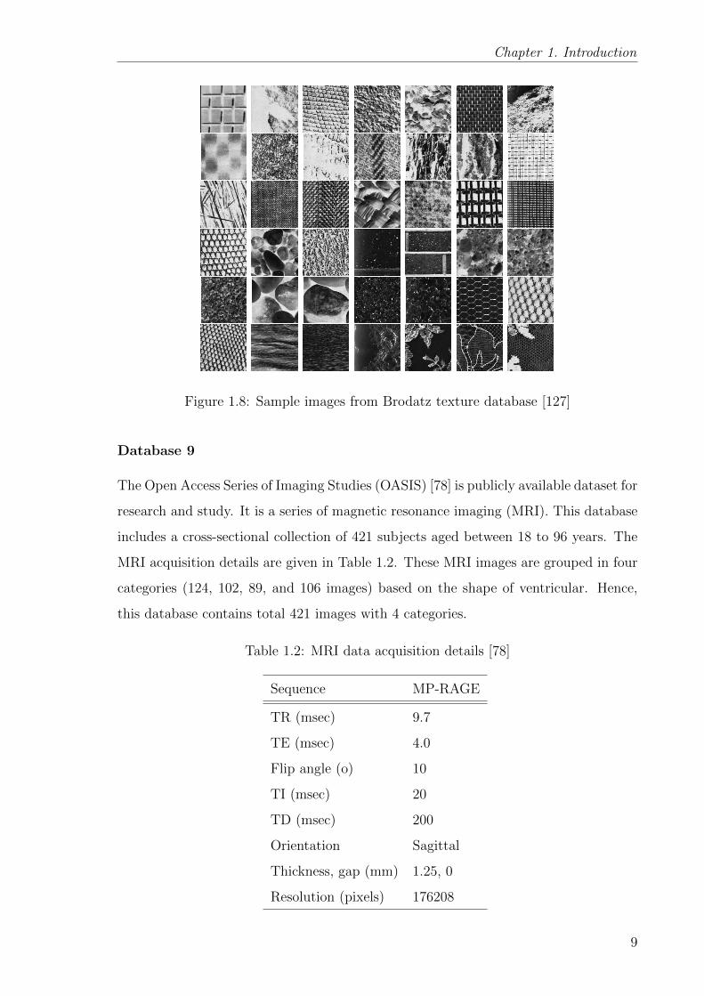
Figure 1.8: Sample images from Brodatz texture database [127]
Database 9
The Open Access Series of Imaging Studies (OASIS) [78] is publicly available dataset for
research and study. It is a series of magnetic resonance imaging (MRI). This database
includes a cross-sectional collection of 421 subjects aged between 18 to 96 years. The
MRI acquisition details are given in Table 1.2. These MRI images are grouped in four
categories (124, 102, 89, and 106 images) based on the shape of ventricular. Hence,
this database contains total 421 images with 4 categories.
Table 1.2: MRI data acquisition details [78]
Sequence MP-RAGE
TR (msec) 9.7
TE (msec) 4.0
Flip angle (o) 10
TI (msec) 20
TD (msec) 200
Orientation Sagittal
Thickness, gap (mm) 1.25, 0
Resolution (pixels) 176208
9

1.2 Content based image retrieval
Figure 1.9: STex color texture database sample images [65]
Figure 1.10: OASIS Database sample images [78]
10

Chapter 1. Introduction
Database 10
The Olivetti Research Ltd (ORL) database of faces is created by AT&T laboratories,
Cambridge [5]. Images present in this database, have been taken between April 1992
and April 1994. It contains images of 40 users and each user have 10 images. For
some users, the images were taken at different times, with different facial expression,
varying the lighting and with glasses or without glasses. The size of each image in this
database is 92× 112. Sample images from each category has been shown in Fig. 1.11.
Figure 1.11: ORL Database sample images [5]
1.2.2 Query image
Query image represents a sample image for what kind of images user wants to retrieve
from the existing database. Query image can be an any random image and used to re-
trieve similar images. This is called as query by example. To evaluate the performance
of a CBIR system, query can be used as a database image itself. Query image can be
formed by a sketch also.
11

1.2 Content based image retrieval
1.2.3 Feature extraction
Feature extraction is an effective step in image retrieval and its importance depends on
how precisely the feature extraction technique suits on image database taken. There
are two types of features called low level and high level features. Color, shape, texture,
etc. include low level features and conceptual, text descriptor are high level features.
Low level features may be local or global descriptors.
Proposed feature extraction method in this work are as follows and described in
further chapters:
1. Wavelet based local features
2. Color-texture feature
3. Integration of two texture features
4. Local information based texture features
5. Hierarchical color-texture feature
1.2.4 Similarity measure
Feature extraction has to be done for all the images of database and query image,
and a feature vector database has been constructed for the full image database. After
applying the feature extraction process, similarity has been performed for query image.
The following distance measures have been used for the similarity match.
d1 distance
D(dbk, q) =L∑
m=1
∣∣∣∣ Fdbk(m)− Fq(m)
1 + Fdbk(m) + Fq(m)
∣∣∣∣ (1.1)
Euclidean distance
D(dbk, q) =
(L∑
m=1
∣∣(Fdbk(m)− Fq(m))2∣∣) 1
2
(1.2)
Manhattan distance
D(dbk, q) =L∑
m=1
|Fdbk(m)− Fq(m)| (1.3)
12

Chapter 1. Introduction
Canberra distance
D(dbk, q) =L∑
m=1
∣∣∣∣Fdbk(m)− Fq(m)
Fdbk(m) + Fq(m)
∣∣∣∣ (1.4)
Chi-square distance
D(dbk, q) =1
2
L∑m=1
(Fdbk(m)− Fq(m))2
Fdbk(m) + Fq(m)(1.5)
where D(dbk, q) measures the distance between kth database image dbk and the
query image q. Length of the feature vector is denoted by L, and Fdbk and Fq are the
feature vectors of kth database image and the query image respectively.
1.2.5 Evaluation measure
Precision and recall are used to observe the performance of the CBIR system. The
precision of the system represents a ratio of the number of relevant images in retrieved
images and the total number of retrieved images from the database. In the same
manner, recall gives the proportion of the number of relevant images in retrieved images
and the total number of relevant images in the database. For a given query image i, if
total n images are being retrieved, then precision and recall can be calculated as:
P (i, n) =Number of relevant images retrieved
n(1.6)
R(i, n) =Number of relevant image retrieved
Nic
(1.7)
where Nic indicates the total number of relevant images in the database, i.e., number
of images in each category of the database. Average precision and average recall are
formulated as:
Pavg(j, n) =1
Nic
Nic∑i=1
P (i, n) (1.8)
Ravg(j, n) =1
Nic
Nic∑i=1
R(i, n) (1.9)
where j denotes the number of categories. Finally, total precision and total recall for
the whole database are calculated as:
Ptotal(n) =1
Nc
Nc∑j=1
Pavg(j, n) (1.10)
13

1.2 Content based image retrieval
Rtotal(n) =1
Nc
Nc∑j=1
Ravg(j, n) (1.11)
where Nc is the number of total categories exist in the database. Precision and recall
are strong evaluation measures but F-measure combines them in a harmonic mean.
F-measure is defined as a relation between both precision and recall, and it gets larger
when both precision and recall are large. F-measure on the basis of precision and recall,
is calculated as follows:
F =2× precision× recallprecision+ recall
(1.12)
The average normalized modified retrieval rate (ANMRR) is used by the MPEG group
to evaluate the performance of a system [77]. For a given query image Q, total number
of relevant images in the database (ground-truth values) are Ng(Q). Rank of each
ground-truth value for query Q is defined as Rank1(i), i.e., position of the ground-
truth image i in retrieved images. Moreover, a variable K(Q) > Ng(Q) is defined as a
limit of ranks. In retrieved images, a ground-truth value that has a rank greater than
K(Q) is considered as a miss and a new rank, Rank(Q) is defined as follows:
Rank(i) =
Rank1(i) if Rank1(i) ≤ K(Q)
1.25×K(Q) if Rank1(i) > K(Q)(1.13)
K(Q) = min(4×Ng(Q), 2×max(Ng(Q), ∀Q)) (1.14)
Average rank (AVR) can be defined as:
AV R(Q) =1
Ng(Q)
Ng(Q)∑i=1
Rank(i) (1.15)
Modified retrieval rank (MRR) and normalized modified retrieval rank (NMRR)
for different ground-truth values are defined as:
MRR(Q) = AV R(Q)− 0.5× [1 +Ng(Q)] (1.16)
NMRR(Q) =MRR(Q)
1.25×K(Q)− 0.5× (1 +Ng(Q))(1.17)
Average normalized modified retrieval rank (ANMRR) is average of NMRR for different
queries.
ANMRR =1
NQ
NQ∑q=1
NMRR(q) (1.18)
14

Chapter 1. Introduction
where NQ is number of query images. ANMRR value lies between 0 and 1, and AN-
MRR value more close to 0 indicates that more ground-truth results found in retrieval.
Further explanation about ANMRR can be found in [77].
1.2.6 Relevance feedback
CBIR system provides the results based on feature extraction and feature matching.
Relevance feedback is a technique that takes user feedback and improvised the results.
It is a supervised learning technique that helps in upgrading the performance of the
system. It works as a mapping between low level features to conceptual features based
on user requirement. Low level features are directly related to image contents, e.g.,
color, shape, texture. Feedback from user itself leads a CBIR system from low level to
high level semantics. In the relevance feedback process, the query image is modified
based on user feedback and again retrieval technique is processed for better results.
1.3 Object tracking
Object tracking is a crucial issue in the field of pattern recognition and computer vision.
It mainly finds applications in the areas of vehicle navigation, traffic monitoring, face
tracking, etc. Object tracking includes tasks such as object detection in frame, object
feature extraction and object tracking using features.
Object detection is the process of finding notable items of real-world objects such
as cars on road, faces in crowd, planes in the sky, and buildings in images or videos.
Object detection algorithms also use image features and learning algorithms to detect
instances of an object category. Next task is of feature extraction of detected object and
it depends on the category of video and detected objects. Color, object shape, texture,
object orientation and other related features can be utilized as the requirement of video
in this step. Tracking is the key step in object tracking process. Tracking algorithm
chases the object of user interest in further frames. In the presented thesis work, a
problem of object tracking is solved and a novel texture feature is proposed.
15

1.4 Shot boundary detection
1.4 Shot boundary detection
Video is a four dimensional data, and it is a collection of images with some temporal
relation in between sequential images. A video scene is made of some shots, and shots
contain similar images. Keyframe is a frame which is assumed to contain most of the
information of a shot. Keyframe may be one or more according to the requirement of
the system. Shot detection and key frame selection are the initial stages of a video
retrieval model system. It is near impossible to process a video for retrieval or analysis
task, without key frame detection. Key frame detection appears to reduce a large
amount of data from video that makes it easy for further process. In this work, a
shot boundary detection problem is solved using hierarchical approach for color and
texture features. Hierarchical technique is used as a two step approach to remove the
redundant information of keyframes.
1.5 Literature survey
A numerous methods have been proposed in low level and high level image feature
extraction by researchers to enhance the accuracy and reduce the computation in image
retrieval. The proposed work in this thesis is related to low level feature extraction in
different applications, hence, a brief literature survey has been given which is able to
describe visual descriptors.
1.5.1 Color features
Color is a captivating feature of image and very eye-catching for human. Feature for
color images extract the information regarding color distribution. Different color spaces
(RGB, HSV, YCbCr, etc.) retain different kind of color distribution that can be used
to extract a variety of color features. Swain and Ballard presented the idea of color
histogram, and distance measure for image matching via histograms [141]. Two new
schemes were presented by Stricker and Orengo for color indexing in that, first holds
complete color distribution, and second contains only major features instead of full
distribution [139]. For both color and texture information, standard wavelet transform
and Gabor wavelet transform were combined with color histogram and applied for
16

Chapter 1. Introduction
image retrieval [86]. Further, new color feature has been proposed using co-occurrence
and clustering. Lin et al. proposed three features, that are color co-occurrence ma-
trix (CCM), difference between pixels of scan pattern (DBPSP) and color histogram
for K-mean (CHKM), in which CCM and DBPSP are related to color and texture,
and CHKM corresponds to the color feature [68]. Integrated color and intensity co-
occurrence matrix has been proposed for color and texture features. Composition of
color and texture features have been computed in it rather than separation. Instead of
RGB, HSV color space is used for color representation, and this method is applied for
image retrieval in large, labeled and unlabeled image database [147].
Color histogram considers the frequency of each intensity but it does not handle the
spatial co-relation of colors. To overcome this issue, color correlogram was proposed
and it considers the spatial co-relation of color intensity in the image [45]. Again, color
correlogram was used for feature vector, and also a relevance feedback technique has
been applied for supervised learning in two ways, first is improving the query image,
and the second is learning the distance metric and applied for improved result in image
retrieval [44]. Color coherence vector was introduced for image retrieval which uses
coherence and incoherence of image pixel colors, and compared with color histogram
for image retrieval [113].
1.5.2 Texture features
Texture is a prominent feature of image and it has been useful in many pattern recog-
nition applications. Texture is defined by small repeated patterns in image. Gray level
co-occurrence matrix (GLCM) first introduced by Haralick, and it is a very popular
method for extracting statistical features of the image [40]. GLCM is a matrix, that
depends on the co-occurrence of every two pixels in image. Haralick calculated the sta-
tistical features of GLCM for texture feature extraction. GLCM was applied directly
to the image to calculate the features, but Zhang et al. used edge image to extract
more precise information using GLCM in texture images [177]. They applied the Pre-
witt edge detector in four directions and calculated GLCM of edge images, and used
statistical features of co-occurrence matrices for texture image retrieval. GLCM was
extended to single and multi-channel co-occurrence matrix for RGB and LUV color
channels, and applied for color texture image retrieval [108]. Partio et al. used gray
17

1.5 Literature survey
level co-occurrence matrix with statistical features for rock texture image retrieval
[111]. Gaussian smoothing and pyramid representation were utilized for extracting
multi-scale images, and GLCM is applied to the obtained multi scale images, and sta-
tistical features were calculated for image retrieval by Siqueira et al. [123]. Further,
GLCM was broadly used for different applications [12, 62, 28].
1.5.3 Local features
Local features provide each pixel’s local information that is useful to detect texture
patterns in images. Ojala et al. presented local binary patterns (LBP), which proved
its excellence and standard in many areas as a feature descriptor [105]. Local binary
pattern was modified into uniform and rotation invariant local binary pattern [106].
Translation, rotation and scale invariant method using color and edge has been pro-
posed for color-texture and natural image retrieval [168]. LBP compares all neighboring
pixels with center pixel, but Heikkil et al. presented center symmetric local binary pat-
terns (CSLBP) which computes the difference in four directions [42]. Tan and Triggs
proposed local ternary pattern (LTP), that compares neighboring pixels and center
pixel with a threshold interval, and assign a ternary pattern (1, 0, -1). Further, it is
converted into two binary patterns (0, 1), and this method is applied for face recog-
nition [144]. LBP and LTP were based on all neighboring pixels evenly. A direction
based method called directional local extrema pattern (DLEP) has been proposed for
directional edge information in 0◦, 45◦, 90◦ and 135◦ directions, and applied for image
retrieval [95]. Local extrema pattern has been proposed by Murala et al., and joint
histogram of color and LEP has been applied for object tracking [93].
Moment based local binary pattern has been proposed, in which LBP has been
derived from momentgrams, and momentgrams have been constructed from moment
invariants of original image [109]. Zhang et al. proposed local derivative pattern (LDP)
[175], which is a higher order local binary pattern, and used for face recognition. Lo-
cal ternary co-occurrence patterns (LTCoP) have been proposed for medical image
retrieval, that utilize the properties of LTP and LDP [87]. A method based on edge
distribution using local pattern was proposed, and called local maximum edge binary
pattern (LMEBP). It was obtained by considering the magnitude of local difference
between the center pixel and reference eight neighborhood pixels in descending order,
18

Chapter 1. Introduction
and LMEBP was obtained for all eight neighbor pixels. LMEBP was applied for im-
age retrieval and object tracking [85]. Further, LMEBP is extended by Jasmine and
Kumar [49], in which only first three uniform and rotational invariant LMEBPs were
considered as feature vector, also an HSV color histogram was used for feature vec-
tor, and finally joint histogram was constructed for image retrieval. After local binary
pattern and local ternary pattern, Murala et al. proposed local tetra patterns (LTrP)
which took advantage of vertical and horizontal directional neighborhood of each pixel
and constructed a tetra pattern, which was again converted into binary patterns [96].
They combined it with Gabor transform, and applied it for image retrieval. Jacob
et al. extended local tetra patterns in RGB color channels. For each center pixel of
a particular color channel, other color channels were used for horizontal and vertical
direction pixels, and applied it for image retrieval [51].
1.5.4 Biomedical image retrieval
Content based image retrieval might be beneficial in medical imaging for handling
large image database. It can be very useful for medical students and interns to learn
disease by retrieving similar images corresponding to a particular image. Medical
image retrieval has been performed using an open source system (GNU Image Finding
Tool) with some improvement using histogram and Gabor filters [83]. Discrete sine
transform is used for feature extraction and ’Boosting’ method is applied for increasing
the accuracy of the system [63]. Image retrieval has been performed using wavelet
transform with Daubuchies, Haar and Gabor wavelets, and statistical features have
been extracted for magnetic resonance image retrieval [146]. The directional binary
wavelet pattern has been proposed for face and biomedical image retrieval using binary
wavelet and local binary pattern [94]. Felipe et al. proposed medical image retrieval
using gray level co-occurrence matrix in 0◦, 45◦, 90◦ and 135◦ directions, and 1, 2, 3, 4
and 5 distances [34]. Further, feature vector has been obtained from GLCM.
Murala et al. proposed local mesh pattern (LMeP) for biomedical image retrieval
and indexing. It creates a local pattern using the mesh of neighboring pixels [90]. Peak
valley edge patterns were proposed for medical image retrieval that extracts directional
edge information using first order derivative [88]. Local mesh patterns and peak valley
19

1.5 Literature survey
edge patterns were combined into local mesh peak valley edge patterns and proposed
for MRI and CT image indexing and retrieval [91].
1.5.5 Object tracking
Object tracking in a moving camera for non-rigid objects has been performed with
mean shift tracking algorithm and dissimilarity has been measured with a distance
measure derived from Bhattacharya coefficient [21]. For better object tracking, shadow
detection and suppression have been carried out using the HSV color information of
moving objects [25]. A kernel based object tracking was employed for non-rigid objects
using histogram as a feature space [22]. Shape features were also utilized with HSV
color histogram using edge histogram in different directions and applied to object
tracking [131]. An interest point based tracking algorithm was proposed by Babu and
Parate [11]. Texture recognition has been applied in the temporal domain for a dynamic
sequence using local binary pattern in three orthonormal planes [179]. A modified LBP
illumination variation was proposed and applied to detect moving objects in a video
sequence [41]. Takala et al. used color histogram, color correlogram and local binary
pattern for color and texture features. Motion features were extracted using trajectories
and applied for object tracking in indoor and outdoor videos [143].
Object tracking in illumination, occlusion and object/camera motion conditions
has been proposed using local features [115]. A two layer feature learning module has
been proposed using neural network and pre-learned features have been been adopted
in tracking mode in video sequence [157]. Joint color texture histogram created by
LBP and RGB color channel, is used to extract feature and mean shift algorithm
is applied for object tracking [102]. A novel method called, spatial extended center
symmetric local binary pattern was proposed for background subtraction from the
image sequence [164]. Local maxima edge binary pattern (LMEBP) has been proposed,
and rotation invariant uniform LMEBP has been applied for object tracking using mean
shift tracking algorithm [85]. Dash et al. proposed a method based on local binary
patterns and Ohta color features instead of RGB, and employed it for object tracking
[27]. Multiple object tracking in a long sports video was proposed by Liu et al. using
short-term activity of each player in the game [69].
20

Chapter 1. Introduction
1.5.6 Shot detection
A video shot transition happens in two ways, i.e., abrupt and gradual transition. The
abrupt transition happens because of short cuts and gradual transition includes shot
dissolve and fades. Many algorithms have been proposed to detect abrupt and gradual
shot transition in video sequence [15]. A hierarchical shot detection algorithm was
proposed using abrupt transitions and gradual transitions in different stages [16]. Wolf
and Yu presented a method for hierarchical shot detection based on different shot tran-
sition analysis and used multi-resolution analysis. They used a hierarchical approach to
detect different shot transitions, e.g., cut, dissolve, wipe-in, wipe-out, etc. [172]. Local
and global feature descriptors have been used for feature extraction in shot boundary
detection. Apostolidis et al. used local Surf features and global HSV color histograms
for gradual and abrupt transitions for a shot segmentation [9].
Images are still and generally spatial information are extracted for analysis pur-
pose. However, for a video study, temporal information should be recognized with
spatial information. Temporal information defines the activity and transition of a
frame to another frame. Rui et. al. proposed a keyframe detection algorithm using
color histogram and activity measure. Spatial information was analyzed using color
histogram and activity measure is used for temporal information detection. Similar
shots are grouped later for better segmentation [125]. A two stage video segmentation
technique was proposed using a sliding window. A segment of frame is used to detect
shot boundary in first stage, and in second stage, the 2-D segments are propagated
across the window of frames in both spatial and temporal direction [119]. Tippaya et
al. proposed a shot detection algorithm using RGB histogram and edge change ratio,
and three different dissimilarity measures have been used to extract difference between
frame feature vectors [145].
Event detection and video content analysis have been done based on shot detection
and keyframe selection algorithms [23]. Similar scene detection has been done using
clustering approach. Story line has been made from a long video [169]. Event detection
in sports video has been analyzed using long, medium and close-up shots, and play
breaks are extracted for summarization of a video [32]. A shot detection technique has
been implemented based on visual and audio content in video. Wavelet transformation
domain has been utilized for feature extraction [97].
21

1.6 Objective
1.6 Objective
The main objective of this thesis is to introduce feature extraction methods for com-
puter vision applications that includes content based image retrieval, object tracking
and shot boundary detection. Many methods for low level features have been proposed
by researchers as explained in Literature survey section. This thesis work is concen-
trated on local feature extraction methods using neighboring intensities of image pixels.
Extended versions of traditional LBP are proposed with respect to orientation of pix-
els, co-occurrence of pixel pairs, neighboring pixels mutual relationship, etc. Targeting
towards better feature extraction methods with respect to accuracy, the objectives of
this work are as follows:
• Traditional LBP and its extended versions target to extract local pattern related
to neighboring and center pixels and convert the pattern map into a histogram to
create a feature vector. Local pattern map contains more information that can
not be summarized using histogram. To extract more information, co-occurrence
of pixel pairs are used in this work. Co-occurrence provides mutual occurrence
of pixel pairs instead of occurrence of each patterns (histogram) in the pattern
map.
• Local information based on pixels in different direction can give more detailed
features than traditional LBP. Design of a feature extraction method for image
retrieval based on different directions is targeted in this work.
• Mostly local patterns proposed in literature use relationship of neighboring pixels
with center pixel. There is a need to design a local pattern that can extract
mutual relationship between neighboring pixels. This problem is solved using a
novel local pattern in this thesis.
• A problem to track an object is addressed using a novel local pattern. The
proposed local pattern aims to extract directional information using less pixels
that results in a reduced feature vector length.
• Shot boundary detection and keyframe extraction are problems to reduce a video
into few frames so that it can be used for further processing. A video scene may
22

Chapter 1. Introduction
contain many repeating shots in nonconsecutive manner and a direct approach
to extract keyframes may lead to redundant keyframes in this scenario. In this
work, main aim to solve the problem of shot boundary detection is to reduce
redundant information from a video summary using a hierarchical approach.
1.7 Organization of the thesis
This thesis presents novel low level image descriptors and integration of different image
features. The whole work has been organized in nine chapters. Chapter 2 suggests two
new proposed feature descriptors using discrete wavelet transform (DWT) and local
patterns. Murala et al. proposed local extrema pattern (LEP) [93] and directional local
extrema patterns (DLEP) [95] for object tracking and image retrieval respectively. In
the proposed work, two techniques have been established to extract local features from
the wavelet transformation domain. In the first method, two level DWT has been
applied to the original image, and seven sub-band images have been obtained. To
extract local features, local extrema patterns have been extracted, and histograms of
all LEP maps have been created. In the second method, one-level DWT is applied
to the image. Four sub-band images, approximation, horizontal, vertical and detail
sub-band, are obtained. DLEP is a directional method and works in four directions,
i.e., 0◦, 45◦, 90◦, 135◦. All four DLEPs are applied on DWT sub-band images in a way
that maximum directional information can be obtained. Both methods are tested on
Corel-5k and Corel-10k databases [2]. Precision and recall are obtained to verify the
performance of presented methods. Both techniques are compared with some existing
local patterns, and it has been observed that both the techniques are better from
others.
Chapter 3 focuses on a feature extraction method that handles color and texture
information together. In this chapter, we have proposed a novel feature descriptor,
called local extrema co-occurrence pattern. Each image in the database is converted
into HSV color space from RGB color space, since HSV color space gives information
about hue, saturation and value separately. Quantized color histograms of hue and
saturation components are calculated for color information of image. Local extrema co-
occurrence pattern is applied to the value component to extract the texture information.
23

1.7 Organization of the thesis
Further, this method is applied to three natural image databases and two texture image
databases. Corel-1k [1], Corel-5k [2], Corel-10k [2], MIT VisTex color-texture database
[3] and STex database [65] are used to determine the performance of the method.
Moreover, this method is compared to some other local patterns with color histogram.
Evaluation measures, e.g., precision, recall and F-measure are used to validate the
performance of the proposed method as compared to other methods.
Chapter 4 focuses on a problem of a multi-purpose feature descriptor on different
category databases. Heikkila et al. proposed CSLBP that utilizes only center sym-
metric pixels to create the local pattern [42]. They have used histogram to create the
feature vector of CSLBP. Histogram only utilizes the information of occurrence of each
pattern value in the pattern map. In the proposed method, co-occurrence of every
pixel pair is observed in different directions and feature vector is made accordingly.
CSLBP is applied on the original image and pattern map is obtained. GLCMs of two
different distances and four different directions have been applied on pattern map and
combined in different ways. Final feature vector is obtained by combining four GLCMs
of different direction and distance. This method is applied on two texture (MIT Vis-
Tex database [3] and Brodatz database [127]), one face (ORL face database [5]) and
one MRI image database (OASIS MRI database [78]). This method is compared with
the existing local patterns for performance measurement. Precision and recall curves
proved the accuracy of the proposed method.
Chapter 5 discusses the problem of texture and face image retrieval. A novel feature
descriptor called, local tri directional pattern is proposed which extracts information
of each pixel in image using neighboring pixels. Nearest neighborhood of 8-pixels
are considered for pattern creation. Three most adjacent pixels of each neighboring
pixel are taken for pattern formation. Based on their difference with corresponding
neighboring pixel, a tri-directional pattern is formed. Further, this pattern is converted
into binary pattern. For more information, a magnitude pattern is also combined with
LTriDP, and histograms of both patterns are concatenated. This algorithm is applied
for texture and face image retrieval using Brodatz texture database [127], MIT VisTex
database [3] and ORL face database [5].
Chapter 6 presents a novel feature extraction method called, local neighborhood
difference pattern (LNBD). LBP analyzes the relationship of center pixel with neigh-
24

Chapter 1. Introduction
boring pixels. In the proposed method, the mutual relationship of neighboring pixels is
considered. Relationship of each neighboring pixel with two other neighboring pixels is
observed, and converted into a binary pattern map. For more information, LBP (center-
neighborhood pixel relationship) and LNBD (neighboring pixels mutual relationship)
are combined in one feature vector. The proposed method is applied to Corel-10k
database [2], MIT natural scene database [4], Brodatz texture database [127] and STex
database [65] for image retrieval purpose. Precision and recall curves are measured for
the proposed method and for other existing methods. Evaluation curves show that the
proposed method outperforms others.
Chapter 7 discusses the problem of object tracking in a video sequence. Object
tracking problem using color and texture information is considered in this chapter. A
novel texture descriptor, local rhombus pattern (LRP), is proposed in this work. LRP
considers the four neighboring pixels which come under the rhombus of the center
pixel. Local relationship of these four pixels with other four neighboring pixels has
been obtained using differences, and a binary pattern has been constructed. HSV color
histogram is acquired for color information, and joint histogram is obtained of HSV
color and LRP. The proposed method is tested on traffic video and sport video.
Chapter 8 presents a problem of shot detection in video sequences. The main
motivation of this problem is to eliminate redundant shots and extract keyframes.
In the proposed work, hierarchical shot detection algorithm has been developed in
two stages. First stage extracts temporal information of video and detect the initial
shot boundary and extract the keyframes based on each shot. In the second stage,
spatial information of extracted key frames from first stage are analyzed, and redundant
keyframes are excluded. Keyfarmes extraction provided using entropy of each frame in
video. Experiments have been done on news, movie clip and TV advertisement video.
Experiment results show major difference in the number of key frames extracted in
first and final stage of the process.
Chapter 9 concludes the work done in all above chapters. It presents the perfor-
mance of the proposed methods over existing methods in terms of accuracy. Also,
future work using the proposed methods in different applications have been described.
25


Chapter 2
CBIR System using Discrete Wavelet
Transform and Local Patterns
Content based image retrieval is grievous need of present scenario in digital imaging
world. Modern advancement in technology and evolution of digital images force to
create vigorous and methodical systems for searching and retrieving images. Content
based image retrieval is a solution for this troublesome problem. Many methods have
been proposed based on statistics, transformations and local patterns to achieve this
task.
In 1982, Jean Morlet initiated the idea of wavelet transform. Discrete wavelet trans-
form (DWT) is the decomposition of signal into four sub bands which are obtained by
applying low pass and high pass filters. It is used in signal processing, image de-
noising, fingerprint verification, speech recognition along with others [133]. In feature
extraction methods, local patterns have made their place because of their efficiency and
simplicity. However, most of the local patterns have been extracted from the original
image. The main motivation of the presented work is to extract local patterns from
the transformation domain to get more information.
27

2.1 Preliminaries
In this chapter, two new content based image retrieval schemes have been discussed.
Local features have been acquired from the transformation domain. Discrete wavelet
transform has been used to obtain sub-band images. Local features using local extrema
pattern (LEP) [93] and directional local extrema pattern (DLEP) [95] have been ex-
tracted from the DWT domain. DLEP extracts features from four directions. Local
feature extraction from transformation domain gives more robust features as compare
to the original image and it has been proved in experimental section of this chapter.
These methods have been tested on massive natural image databases for image retrieval
purpose. These methods are compared with some local feature extraction methods for
validation of accuracy.
2.1 Preliminaries
2.1.1 Discrete wavelet transform
Figure 2.1: 1-level discrete wavelet transform example
The wavelet transform is a modified and improved version of Fourier transform.
The Fourier transform is generated from sinusoid functions and wavelet transform is
generated from wave functions that are called wavelets. Two dimensional discrete
wavelet transform decomposes an image into 4 parts using low and high pass filters.
28

Chapter 2. CBIR System using Discrete Wavelet Transform and Local Patterns
Filters are first applied to one dimension (row-wise) and then other (column-wise)
as shown in Fig. 2.2. After filtering process, down-sampling has to be done for re-
ducing the computation. In this process, four sub-band images are retrieved, which
are called approximation, horizontal, vertical and detail parts. This is called one level
decomposition. For next level, again same process is applied on 1-level approximation
part.
L(x)
H(x)
2
2
L(y)
H(y)
L(y)
H(y)
2
2
2
2
I(x,y)
Approximation
Horizontal
Vertical
Diagonal 2
2
2
2
2
row-wisecolumn-wise
Figure 2.2: 2-dimensional filter bank and downsampling process for 2d-DWT
2.1.2 Local extrema pattern
75 40 10051 78 8590 62 80
8 4 216 132 64 128
0 0 10 11 0 1
0 0 20 163 1
32 0 128
-3 -38 22-27 712 -16 2
0 1 10
8 4 21
0 4 26 0
75 40 10051 78 8590 62 80
-3 -38 22-27 712 -16 2
Figure 2.3: Local Extrema Pattern
Local extrema pattern is a local feature descriptor in which, pattern value depends
on particular direction’s neighboring pixels [93]. LEP operator finds the difference
between center and its neighbor pixels, and based on the value of difference in four
different directions (0◦, 45◦, 90◦ and 135◦), it decides the value of pattern. If both are
of same sign, it gives 1 and if both are of different sign it gives 0. LEP of the center
pixel is obtained as follows:
I ′k = Ik − Ic; k = 1, 2, . . . , 8 (2.1)
29

2.1 Preliminaries
I ′k(θ) = F1(I′j, I′j+4); j = (1 + θ/45)
∀θ = 0◦, 45◦, 90◦, 135◦(2.2)
F1(I′j, I′j+4) =
1 I ′j × I ′j+4 ≥ 0
0 else
LEP (Ic) =∑θ
2θ/45 × I ′k(θ)
∀θ = 0◦, 45◦, 90◦, 135◦(2.3)
where Ic and Ik are center and neighbor pixel. The direction angle of LEP is denoted
by θ. Feature vector is obtained using histogram of LEP image.
Hist(L) |LEP =m∑j1=1
n∑j2=1
F2(LEP(j1, j2), L);
L ∈ [0, 15]
(2.4)
F2(x1, x2) =
1 x1 = x2
0 else(2.5)
where L is intensity in LEP map. The illustration of LEP is given in Fig. 2.3.
2.1.3 Directional local extrema pattern
The directional local extrema pattern (DLEP) is proposed by Murala et al. for content
based image retrieval [95]. DLEP operator compares the neighboring pixels of four
directions (0◦, 45◦, 90◦, 135◦) with center pixel, and assigns the binary pattern that
depends on the relationship of pixels in 0◦, 45◦, 90◦ and 135◦ directions. Mathematical
formulation of DLEP is given below.
Fθ(Ic) = F1(I′j, I′j+4) ∀ j = (1 + θ/45)
∀θ = 0◦, 45◦, 90◦, 135◦
DLEPpat(Ic))|θ = {Fθ(Ic); Fθ(I1); Fθ(I2); . . . Fθ(I8)}
DLEP(Ic)|θ =8∑
k=0
2k ×DLEPpat(Ic)|θ(k) (2.6)
where I ′j is defined as Eq. 2.1. Ic and Ii are center and neighborhood pixels. θ denotes
the direction angle of DLEP. Histogram is used for calculating the feature vector. The
30

Chapter 2. CBIR System using Discrete Wavelet Transform and Local Patterns
21 57 3 9 2925 11 45 10 1112 3 24 41 131 19 13 36 4021 40 31 2 59
21 57 3 9 2925 11 45 10 1112 3 24 41 131 19 13 36 4021 40 31 2 59
21 57 3 9 2925 11 45 10 1112 3 24 41 131 19 13 36 4021 40 31 2 59
21 57 3 9 2925 11 45 10 1112 3 24 41 131 19 13 36 4021 40 31 2 59
21 57 3 9 2925 11 45 10 1112 3 24 41 131 19 13 36 4021 40 31 2 59
21 57 3 9 2925 11 45 10 1112 3 24 41 131 19 13 36 4021 40 31 2 59
21 57 3 9 2925 11 45 10 1112 3 24 41 131 19 13 36 4021 40 31 2 59
21 57 3 9 2925 11 45 10 1112 3 24 41 131 19 13 36 4021 40 31 2 59
21 57 3 9 2925 11 45 10 1112 3 24 41 131 19 13 36 4021 40 31 2 59
0110
0
1 1 1 1
1 1 1 0DLEP Pattern: 011111110
Figure 2.4: Directional Local Extrema Pattern
illustration of DLEP calculation is shown in Fig. 2.4. Further details about DLEP can
be found in [95].
Hist(L) |DLEP(θ) =m∑i1=1
n∑i2=1
F2(DLEP(i1, i2) |θ, L);L ∈ [0, 511]
2.2 Proposed methods
Two new schemes have been proposed using local patterns and 2D-DWT in this work.
In both the methods, local patterns have been extracted from wavelet transformation
domain.
31

2.2 Proposed methods
2.2.1 Proposed method 1
This work presents a new multi-scale content based image retrieval system which lever-
ages the multi-resolution property of discrete wavelet transform (DWT) and the local
information attribute of local extrema patterns (LEPs). A two level discrete wavelet
transform with Daubechies-4 wavelet filters are applied to the original image and seven
subband images are obtained. Local extrema pattern is performed on these seven sub-
band images, which gives seven local extrema pattern maps. Multi-resolution analysis
using DWT helps in enhancing the features of image. It extracts the information of
image in different directions, and obtain four subband images that carries more direc-
tional information rather than the original image with respect to feature extraction.
LEP works with local intensity and it is also direction based. Consequently, applying
LEP on wavelet subband image makes it possible to extract directional and textural
information from the image that is less possible with the original image.
Histogram is calculated for each map where maximum intensity in each map is 15,
therefore length of each histogram is 16. Joint histogram is obtained by combining all
seven histograms. Resultant length of joint histogram is 16× 7. Feature vector length
of the proposed method is less as compared to other existing methods (LBP, BLK LBP
etc.). Hence, the proposed method is more suitable for pattern recognition application
like image revival, face recognition, etc.
Algorithm
Block diagram of proposed method 1 is illustrated in Fig. 2.5.
Input: Query image.
Output: Similar images.
1. Upload the query image of size m× n.
2. Convert it into gray scale image if it is a color image.
3. Apply 2-level DWT on the image obtained in step 2 and get seven sub band
images.
4. Apply LEP on acquired seven images.
5. Construct the histogram for all seven LEP maps obtained in step 4.
32

Chapter 2. CBIR System using Discrete Wavelet Transform and Local Patterns
ImageDatabase
2-levelDWT Local extremapatterns Histogram Joint Histogram
Feature Vector
SimilarityMeasure
RetrievedImages
Query Image
Feature vectorDatabase
Figure 2.5: Block diagram of the proposed method
6. Concatenate all histograms with equal weights.
7. Compare the histogram of query image and database’s image with the help of
distance formula given in Eq. 1.1 and get distance measure.
8. Sort the distance measure and get the images of minimum distance as the best
results.
2.2.2 Proposed method 2
In the proposed method 2, two dimensional discrete wavelet transform is applied on
original image, and 4 subband images (approximation, horizontal, vertical and detail
parts) are extracted. These four sub images render low pass, 0 degree, 90 degree, 45 and
-45 degrees information respectively, as shown in Fig. 2.1. Daubechies-4 (db4) wavelets
are applied for decomposition, and DLEP algorithm is applied in different directions
on four sub images as mentioned in table 2.1. Both DWT and DLEP, are helpful in the
Table 2.1: Applied DLEP on wavelet coefficient
Approximation part 4-direction DLEP (0◦, 45◦, 90◦, 135◦)
Detail Part 2-direction DLEP (0◦, 90◦)
Horizontal Part 3-direction DLEP (45◦, 90◦, 135◦)
Vertical Part 3-direction DLEP (0◦, 45◦, 135◦)
33

2.2 Proposed methods
extraction of directional features. With the help of the wavelet transform, we extract
different sub images with different directional information, and by applying DLEP of
different directions, feature vector is being extracted. For example, in detail part, only
0◦, 90◦ DLEP is applied because 45◦ and −45◦ degree information are already extracted
in wavelet transform, for horizontal part DLEP of 45◦, 90◦ and 135◦ is applied as the
information of 0◦ has earlier been taken in wavelet transform. The same process is
applied to other sub images, and accordingly DLEP of specific direction is obtained.
In this process, additional directional information is being extracted.
After applying DLEP on four sub images, twelve DLEP maps are extracted and
their corresponding histograms are obtained. A joint histogram is prepared by con-
catenating all 12 histograms one after another. DLEP of each direction gives a feature
vector of the length 512. In the proposed method, twelve DLEP maps (4+2+3+3) of
4 orientations (0◦, 45◦, 90◦, 135◦) are obtained and the total length of joint histogram
is 12× 512.
ImageDatabase
1-levelDWT
Histogram 1
JointHistogram
Feature Vector
SimilarityMeasure
RetrievedImages
Query Image
Feature vectorDatabase
Approximationsubband
Horizontalsubband
Verticalsubband
Detailsubband
0°, 45°, 90°,135° DLEP
45°, 90°, 135°DLEP
0°, 45°, 135°DLEP
0°, 90°DLEP
Histogram 2
Histogram 3
Histogram 4
Figure 2.6: Block diagram of the proposed system
Algorithm
Input: Query image
Output: Retrieved similar images
1. Upload the input image of size m× n.
34

Chapter 2. CBIR System using Discrete Wavelet Transform and Local Patterns
2. If it is color image, then convert it into a gray scale.
3. Apply 1-level DWT on the obtained gray scale image.
(a) Apply 0◦, 45◦, 90◦, 135◦ DLEP on approximation part.
(b) Apply 45◦, 90◦, 135◦ DLEP on horizontal part.
(c) Apply 0◦, 45◦, 135◦ DLEP on vertical part.
(d) Apply 0◦, 90◦ DLEP on detail part.
4. Get histogram of all 12 (4+3+3+2) DLEP maps and concatenate all histograms.
5. Compare the histogram of the query image and the database image with the help
of distance formula and get distance measure.
6. Sort the distance measure and get the minimum distance as the best result.
Both the methods proposed in this chapter are obtained using wavelet transformation
domain. Wavelet coefficients on different scales gives directional information. Wavelets
have been used in feature extraction by researchers. In this work, wavelet coefficients
used to extract local features. Hence, it is advantageous as local features (LEP and
DLEP) also use directional information for feature extraction.
2.3 Experimental results and discussion
To prove the excellence of both the methods, Corel-5k and Corel-10k databases have
been used. Explanation about databases have been given in Chapter 1, Section 1.2.1.
Each image of database have been considered as query image, and the results have
been obtained using evaluation measures, precision and recall (Chapter 1, Section
1.2.5). The proposed methods have been compared with the following methods:
DWT : Discrete wavelet transform
LEP : Local extrema pattern
CS LBP : Center-symmetric local binary pattern
LEPSEG : Local edge pattern for segmentation
LEPINV : Local edge pattern for image retrieval
BLK LBP : Block based local binary pattern
35

2.3 Experimental results and discussion
LBP : Local binary pattern
DLEP : Directional local extrema pattern
Proposed method 1 and 2 are abbreviated as PM1 and PM2 respectively.
2.3.1 Experiment 1
Results of Corel-5k has been demonstrated in this experiment section. Two kinds of
plots for each precision and recall are presented here. One is based on the number
of images retrieved and other one is according to the category of images. Graphs of
both the methods have been demonstrated and compared with other existing methods.
In experiments, 10, 20,..,100 images are retrieved one after another for performance
measurement and, precision and recall are obtained.
Fig. 2.7(a) and 2.7(b) show graphs between total number of images retrieved with
precision and recall. Proposed method 1 is the combination of DWT and LEP, and it
is better in terms of performance from both DWT and LEP. Similarly, the proposed
method 2 is extracted from DWT and DLEP, and it shows high performance when
compare to both DWT and DLEP. Also, both the methods outperform other methods,
and show better performance in terms of accuracy. In Fig. 2.7(c) and 2.7(d), plots
of each category in Corel-5k have been demonstrated with precision and recall. Both
the proposed methods presented better precision recall in most of the categories than
other methods, and all above, PM2 (proposed method 2) is better than PM1 (proposed
method 1).
2.3.2 Experiment 2
In second experiment, Corel-10k database has been used. Similarly, like previous exper-
iment, precision and recall curves have been plotted with number of images retrieved,
and shown in Fig. 2.8. Results of experiments are shown in graphs. Fig. 2.8 ex-
plains the change in recall and precision with a total number of images retrieved, and
proposed methods outperform other methods. Although, PM2 beats PM1 in terms
of precision and recall, PM2 has bigger feature vector length than PM1 that leads to
more time complexity in image retrieval, and it is explained using table 2.3. Fig. 2.8
presents change in recall and precision with category of images. Clearly graphs validate
36

Chapter 2. CBIR System using Discrete Wavelet Transform and Local Patterns
10 20 30 40 50 60 70 80 90 10010
20
30
40
50
60
Number of images retrieved
Pre
cisi
on
DWTLEPCS_LBPLEPSEGLBPINVBLK_LBPLBPDLEPPM1PM2
(a)
10 20 30 40 50 60 70 80 90 1000
5
10
15
20
25
Number of images retrieved
Rec
all
DWTLEPCS_LBPLEPSEGLBPINVBLK_LBPLBPDLEPPM1PM2
(b)
1 3 5 7 9 11 13 15 17 19 21 23 25 27 29 31 33 35 37 39 41 43 45 47 49 500
20
40
60
80
100
Number of category
Pre
cis
ion
(c)
1 3 5 7 9 11 13 15 17 19 21 23 25 27 29 31 33 35 37 39 41 43 45 47 49 500
20
40
60
80
Number of category
Re
ca
ll
DWT LEP CS_LBP LEPSEG LBPINV BLK_LBP LBP DLEP PM1 PM2
(d)
Figure 2.7: Corel-5k database (a) precision and (b) recall, with number of images
retrieved, and (c) precision and (a) recall, with image database category
37

2.4 Conclusion
the efficiency of proposed methods for large Corel-10k image database, and proposed
method outperforms other existing methods in most of the categories.
Total precision and recall have been shown in table 2.2 for the fixed number of
retrieved images. For precision and recall, total 10 and 100 retrieved images are chosen
respectively and the results are presented for all methods including proposed methods.
Proposed method 2 has the best performance measures among these methods.
Feature vector length directly implies the image retrieval time of the system. More
feature vector length takes more time to extract images. In table 2.3, feature vector
length of all the methods have been shown. Evaluation measures have already shown
that the performance of both the proposed methods are better than others. The
proposed method 2 is better than the proposed method 1 in accuracy. However, the
feature vector length of PM1 is less than PM2.
Table 2.2: Precision and Recall percentage for all methods
Method Corel 5k Corel 10k
Precision Recall Precision Recall
DWT 29.06 12.77 23.13 8.96
LEP 41.52 18.23 33.40 13.26
CS LBP 32.97 14.00 26.43 10.15
LEPSEG 41.56 18.31 34.01 13.81
LEPINV 35.19 14.84 28.93 11.22
BLK LBP 45.76 20.30 38.13 15.34
LBP 43.63 19.22 37.62 14.98
DLEP 48.73 21.05 39.99 15.71
PM1 49.32 23.32 40.68 17.91
PM2 51.41 24.12 43.13 18.26
2.4 Conclusion
This chapter proposes two image retrieval methods that extracts features using wavelet
transform domain. Multi-resolution analysis has been done with wavelet transform. In
proposed method 1, discrete wavelet transform is applied on image, and then local
38

Chapter 2. CBIR System using Discrete Wavelet Transform and Local Patterns
10 20 30 40 50 60 70 80 90 1005
10
15
20
25
30
35
40
45
Number of images retrieved
Pre
cisi
on
DWTLEPCS_LBPLEPSEGLBPINVBLK_LBPLBPDLEPPM1PM2
(a)
10 20 30 40 50 60 70 80 90 1000
5
10
15
20
Number of images retrieved
Rec
all
DWTLEPCS_LBPLEPSEGLBPINVBLK_LBPLBPDLEPPM1PM2
(b)
0 5 10 15 20 25 30 35 40 45 50 55 60 65 70 75 80 85 90 95 1000
20
40
60
80
100
Number of category
Pre
cis
ion
(c)
0 5 10 15 20 25 30 35 40 45 50 55 60 65 70 75 80 85 90 95 1000
20
40
60
80
Number of category
Recall
DWT LEP CS_LBP LEPSEG LBPINV BLK_LBP LBP DLEP PM1 PM2(d)
Figure 2.8: Corel-5k database (a) precision and (b) recall, with number of images
retrieved, and (c) precision and (a) recall, with image database category
39

2.4 Conclusion
Table 2.3: Feature vector length of different methods
Method Feature vector length
DWT 20
LEP 16
CS LBP 16
LEPSEG 512
LEPINV 72
BLK LBP 256 × 6
LBP 256
DLEP 512×4
PM1 16×7
PM2 512×12
extrema patterns are extracted from wavelet coefficients. Total seven local extrema
pattern maps have been obtained and histogram is generated. Wavelet transform
captures the low frequency as well as high frequency features that helps local extrema
pattern to create more direction oriented features.
In second method, one level discrete wavelet transform is applied on the image, and
DLEP of different directions obtained from sub-band images. This method utilizes the
directional information of both DWT and DLEP, and combines it in a directive way so
that most of the detail can be extracted from the image for construction of the feature
vector. Effectiveness of the proposed method is measured by testing on Corel-5k and
Corel-10k image database. Proposed methods are compared with some past results,
and evolution measures show that the proposed methods are more accurate than past
methods.
40

Chapter 3
Local Extrema Co-occurrence Pat-
tern for Image Retrieval
In this chapter, we propose a new image retrieval technique; local extrema co-
occurrence patterns (LECoP) using the HSV color space. To utilize the color, intensity
and brightness of images, HSV color space is used in this method. Local extrema pat-
terns are applied to define the local information of image and gray level co-occurrence
matrix is used to obtain the co-occurrence of LEP map pixels. The local extrema
co-occurrence pattern extracts the local directional information from local extrema
pattern, and convert it into a well-mannered feature vector with use of gray level co-
occurrence matrix. Many local patterns for image retrieval have been proposed by
researchers, but most of the local patterns consider the frequency of each pattern in
the image and treat it as a feature descriptor using histogram. However, frequency
gives information about the occurrence of pattern, and it does not reveal any informa-
tion for mutual occurrence of patterns in the image. Mutual occurrence of patterns
is considered in this work. Earlier work with local pattern and color features, con-
sidered texture pattern and color information as individual features. However in this
work, texture feature of local pattern has been extracted using color space component.
41

3.1 Preliminaries
The presented method is tested on five standard databases called Corel, MIT VisTex
and STex database, in which Corel database includes Corel-1k, Corer-5k and Corel-
10k database. Also, this algorithm is compared with previous proposed methods, and
results in terms of precision and recall are shown in this chapter.
3.1 Preliminaries
3.1.1 Color space
In general, images are of three types. First one is the binary image, which contains
only two intensities namely black and white pixels. Second is the gray scale image,
that can have a range of intensities, but only in one band. Next is the color image,
which has multiple bands, and each band contains a range of intensity. Most generally
used, RGB images have three bands called, red, green and blue. In RGB images, three
bands contain information about red, green and blue colors, and hence it is called the
RGB color space. The other one is the HSV color space that stands for hue, saturation
and value.
In HSV, hue component directly related to the color, and a human eye can distin-
guish different colors. Hue is defined as an angle. Saturation represents the brightness
and lightness of color component, and the value shows the intensity of a color, that is
decomposed from the color information of the image. Hue presents an angle from 0 to
360 degrees, and each degree occupies different colors. Saturation is numbered from 0
to 1, as it goes from low to high, intensity of color increases. Value also varies from 0 to
1. Many researchers have shown that HSV color space is more appropriate than RGB
space as in HSV space, color, intensity and brightness can be extracted individually
from images [147, 140, 173]. In this work, images are converted from RGB space to
HSV color space.
3.1.2 Gray level co-occurrence matrix
Gray level co-occurrence matrix transforms an image into a matrix which correspond
to the relationship of pixels in the original image. It calculates the mutual occurrence
42

Chapter 3. Local Extrema Co-occurrence Pattern for Image Retrieval
Pixel pair 1 2 3 41 0 3 1 02 2 2 1 33 0 2 1 04 0 4 0 0
4 2 2 1 21 2 3 3 22 1 3 2 24 2 4 2 41 2 2 4 2
3
Figure 3.1: Gray level co-occurrence matrix computation example
of pixel pairs for a specific distance and in a particular direction. For an input image,
the GLCM is calculated as below.
Gθd(i, j) = ]{((x, y), (a, b)) : I(x, y) = i, I(a, b) = j},
where (x, y), (a, b) ∈ Nx ×Ny
(3.1)
(a, b) = (x+ d× θ1, y + d× θ2)
where Gθd is the gray level co-occurrence matrix of distance d and angle θ. I(x, y)and
I(a, b) are the pixel intensity at position (x, y) and (a, b) and # represents the count
of ((x, y), (a, b)) pixels with satisfying further condition given in Eq. 3.1. Nx and Ny
are horizontal and vertical spacial domains. Values of θ1 and θ2 depend on θ and are
shown in table 3.1.
Table 3.1: Values of θ1 and θ2 corresponding to θ in GLCM
θ θ1 θ2
0◦ 0 1
45◦ -1 1
90◦ -1 0
135◦ -1 -1
An example of GLCM calculation is shown in Fig. 3.1. In Fig. 3.1, first matrix is
image matrix and second matrix is the GLCM. Pixel pair of (2, 2) with distance ‘1’
and angle 0◦ is denoted by red arrow in the first matrix and this pixel pair is occurring
three times in the original matrix, and accordingly in the GLCM at position (2, 2) a
number ‘3’ is occurring. Similarly, for other pixel pairs, GLCM is calculated.
43

3.2 Proposed method
3.2 Proposed method
A new texture feature called local extrema co-occurrence pattern (LECoP) is presented
in this work that extracts the co-occurrence of local extrema pattern (LEP) values.
LEP is a texture feature that is proposed by Murala et al. for object tracking [93] and
it is explained in detail in Chapter 2, Section 2.1.2.
The proposed image retrieval method utilizes both color and texture information
of images. Texture and color both are salient features of an image. HSV color space
has been used for extraction of details of the image in hue, saturation and value parts.
Initially, RGB image is converted into HSV color space [135]. Hue corresponds to the
color component, and varies from 0◦ to 360◦. Each number corresponds to different
color. In the proposed work, three different quantization levels of hue component,
i.e., 18, 36 and 72 have been used, and performance of the proposed method has been
observed. All three quantization schemes divide all colors into different sections so that
optimum color information can be obtained. Similarly, saturation is quantized into 10
and 20 bins for reasonable information extraction. All possible combinations of hue
and saturation have been used, and the performance has been observed on different
datasets in section 4.7. The color histogram has proven its excellence in image retrieval
[141]. The histogram is constructed for both hue and saturation parts.
In the HSV color space, value component is nearly close to the gray scale conversion
of the RGB image, therefore, value component is used for texture extraction. Hue
and saturation are used to extract global information regarding color and brightness
using histogram. Local information of each pixel corresponds to the texture feature
of the image, and it has been extracted using local extrema patterns. LEP is applied
to the value channel of original image. It gives a LEP map same as the image size
with entries from 0 to 15. Histogram extracts the information about the frequency of
intensity, that only implies the occurrence of every pattern in the whole image, and
neglect the information regarding the co-occurrence of pixels. Gray level co-occurrence
matrix reveals the relative occurrence of intensity pairs in the image so that the local
information of occurrence of every pixel pairs in the LEP map can be extracted in the
matrix form. Hence, instead of histogram, GLCM is calculated for LEP map. GLCM
in 0◦ with one distance has been used in this proposed work.
44

Chapter 3. Local Extrema Co-occurrence Pattern for Image Retrieval
Intensity size in LEP map is varying from 0 to 15, hence the size of GLCM in this
case is 16 × 16. Each position in the GLCM matrix represents the occurrence of cor-
responding pixel pair. For histogram concatenation, GLCM is again converted into a
single vector, and a combined histogram is made of hue and saturation quantized bins
and GLCM single vector. Total length of feature vector depends on the quantization
number of hue and saturation part. Feature vector can be normalized with a factor
n, according to the database images. In the proposed work, all databases taken for
experiment, are benchmark databases, therefore, the size of images in databases are
same for a particular database. Normalization factor n can vary, if size of images are
different in a database. Hence, according to the size of images in database, normal-
ization factor is chosen 1000 for database 1 (Corel-1k), and 100 for other databases
(Corel-5k, Corel-10k, MIT VisTex and STex) in experiment section since image size in
database 1 is bigger than other databases.
3.3 Proposed system framework
QueryImage
RGB toHSV color
spaceSaturation
18/36/72bin
quantizedhistogram
LocalextremaPattern
Gray levelco-occurrence
matrix
Histogramconcatena-
tion
Hue
Value
10/20 binquantizedhistogram
Resizematrix tovector
Featurevector
Featurevector
database
Queryimagefeaturevector
Imagedatabase
SimilarityMatch
Results
Figure 3.2: Proposed system block diagram
Algorithm of the system is given below and a block diagram of presented work has
been given in Fig. 3.2 .
Input: Query image.
45

3.4 Experimental results and discussion
Output: Retrieved images from the database.
1. Upload the input image.
2. Convert it from RGB to HSV color space.
3. Quantize the hue and the saturation part into 18/36/72 and 10/20 bins respec-
tively (according to the requirement of database), and construct histograms for
both, hue and saturation.
4. Apply LEP on the value part of HSV color space, and obtain LEP map.
5. Construct GLCM of LEP map.
6. Convert GLCM into a vector form.
7. Concatenate the histograms obtained in step 3 with GLCM vector of step 6, and
construct the final histogram as a feature vector.
8. Use similarity distance measure for comparing the query feature vector and fea-
ture vectors of existing feature database.
9. Sort the distance measure, and produce the corresponding images of the best
match vectors as final results.
3.4 Experimental results and discussion
For experimental purpose, natural and texture image databases of color images have
been utilized in this chapter. Three natural-color image databases (Corel-1k, Corel-5k
and Corel-10k) and two color-texture image databases (MIT VisTex database and STex
Ddatabase) have been used. In experiments, for each query image, different number of
images are retrieved separately, and evaluation measures are calculated for each group
of retrieved images. For evaluation measure, precision, recall and F-measure (Chapter
1 Section 1.2.5) are used for all databases and methods. Proposed method is compared
with some existing methods and the details are depicted in table 3.2.
46

Chapter 3. Local Extrema Co-occurrence Pattern for Image Retrieval
10 20 30 40 50 60 70 80 90 10040
45
50
55
60
65
70
75
80
No. of images retrieved
Pre
cisi
on
%
Wavelet+colorhistCS_LBP+colorhistJoint LEP colorhistJoint colorhistLEPINV+colorhistLEPSEG+colorhistPM
(a)
10 20 30 40 50 60 70 80 90 1000
10
20
30
40
50
60
No. of images retrieved
Rec
all %
Wavelet+colorhistCS_LBP+colorhistJoint LEP colorhistJoint colorhistLEPINV+colorhistLEPSEG+colorhistPM
(b)
Figure 3.3: Results of precision and recall with number of images retrieved of Corel-1k
database
3.4.1 Experiment 1
First experiment is conducted on Corel-1k database and the details about this database
are given in Chapter 1, Section 1.2.1.
Fig. 3.3 shows the performance of the presented method according to the number
of images retrieved. Precision-recall curve and F-measure curve have been shown in
Fig. 3.4, and these indicate that the proposed method is better than other methods.
Table 3.3 shows the numerical results of precision and recall in terms of percentage
along with other methods. In terms of precision, the proposed method accuracy has
been increased from Wavelet+colorhist, CS LBP+colorhist, Joint LEP colorhist, Joint
colorhist, LEPINV+colorhist and LEPSEG+colorhist up to 16.26%, 3.56%, 4.59%,
4.56%, 8.43% and 3.67% respectively.
47

3.4 Experimental results and discussion
Table 3.2: Abbreviation of all methods
CS LBP+colorhist : Center-symmetric local binary pattern [42] + RGB color histogram
LEPSEG+colorhist : Local edge pattern for segmentation [168] + RGB color histogram
LEPINV+colorhist : Local edge pattern for image retrieval [168] + RGB Color histogram
Wavelet+colorhist : Discrete wavelet transform + RGB Color histogram [86]
Joint LEP colorhist : Joint histogram of color and LEP [93]
Joint colorhist : Joint histogram of RGB color
PM : Proposed method
0 0.1 0.2 0.3 0.4 0.5 0.6 0.7 0.8 0.9 1
0.4
0.5
0.6
0.7
0.8
0.9
1
Recall
Pre
cisi
on
Wavelet+colorhistCS_LBP+colorhistJoint LEP colorhistJoint colorhistLEPINV+colorhistLEPSEG+colorhistPM
0 10 20 30 40 50 60 70 80 90 1000
0.1
0.2
0.3
0.4
0.5
0.6
0.7
Number of top matches
F−m
easu
re
Wavelet+colorhistCS_LBP+colorhistJoint LEP colorhistJoint colorhistLEPINV+colorhistLEPSEG+colorhistPM
Figure 3.4: Precision-recall curve and F-measure curve for Corel-1k database
3.4.2 Experiment 2
Corel-5k has been used in the second experiment and the details about this database
are given in Chapter 1, Section 1.2.1.
48

Chapter 3. Local Extrema Co-occurrence Pattern for Image Retrieval
10 20 30 40 50 60 70 80 90 10020
30
40
50
60
70
No. of images retrieved
Pre
cisi
on
%
Wavelet+colorhistCS_LBP+colorhistJoint LEP colorhistJoint colorhistLEPINV+colorhistLEPSEG+colorhistPM
(a)
10 20 30 40 50 60 70 80 90 1005
10
15
20
25
30
35
No. of images retrieved
Rec
all %
Wavelet+colorhistCS_LBP+colorhistJoint LEP colorhistJoint colorhistLEPINV+colorhistLEPSEG+colorhistPM
(b)
1 3 5 7 9 11 13 15 17 19 21 23 25 27 29 31 33 35 37 39 41 43 45 47 49500
20
40
60
80
100
No. of image category
Pre
cis
ion
(c)
1 3 5 7 9 11 13 15 17 19 21 23 25 27 29 31 33 35 37 39 41 43 45 47 49500
20
40
60
80
100
No. of image category
Recall
Wavelet+colorhistCS_LBP+colorhistJoint LEP colorhistJoint colorhistLEPINV+colorhistLEPSEG+colorhistPM
(d)
Figure 3.5: Corel-5k plots of (a) precision and (b) recall, with number of images re-
trieved, and (c) precision and (d) recall, with category number
49
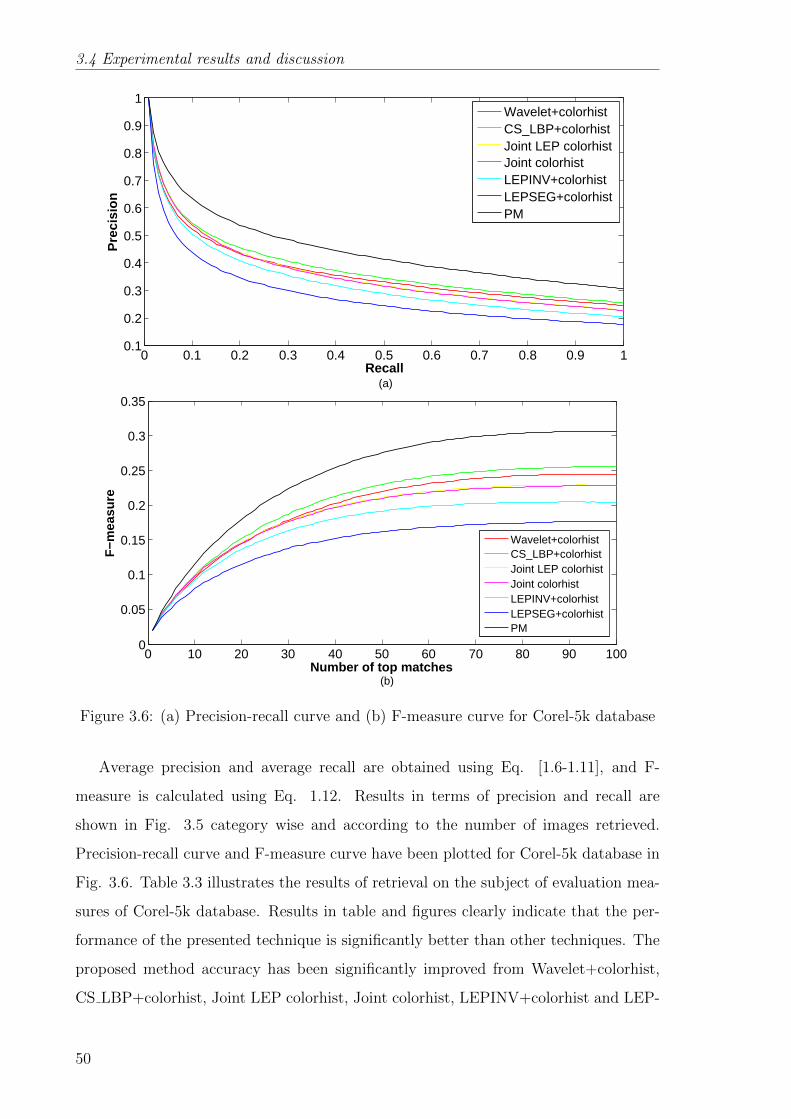
3.4 Experimental results and discussion
0 0.1 0.2 0.3 0.4 0.5 0.6 0.7 0.8 0.9 10.1
0.2
0.3
0.4
0.5
0.6
0.7
0.8
0.9
1
Recall
Pre
cisi
on
Wavelet+colorhistCS_LBP+colorhistJoint LEP colorhistJoint colorhistLEPINV+colorhistLEPSEG+colorhistPM
(a)
0 10 20 30 40 50 60 70 80 90 1000
0.05
0.1
0.15
0.2
0.25
0.3
0.35
Number of top matches
F−m
easu
re
Wavelet+colorhistCS_LBP+colorhistJoint LEP colorhistJoint colorhistLEPINV+colorhistLEPSEG+colorhistPM
(b)
Figure 3.6: (a) Precision-recall curve and (b) F-measure curve for Corel-5k database
Average precision and average recall are obtained using Eq. [1.6-1.11], and F-
measure is calculated using Eq. 1.12. Results in terms of precision and recall are
shown in Fig. 3.5 category wise and according to the number of images retrieved.
Precision-recall curve and F-measure curve have been plotted for Corel-5k database in
Fig. 3.6. Table 3.3 illustrates the results of retrieval on the subject of evaluation mea-
sures of Corel-5k database. Results in table and figures clearly indicate that the per-
formance of the presented technique is significantly better than other techniques. The
proposed method accuracy has been significantly improved from Wavelet+colorhist,
CS LBP+colorhist, Joint LEP colorhist, Joint colorhist, LEPINV+colorhist and LEP-
50
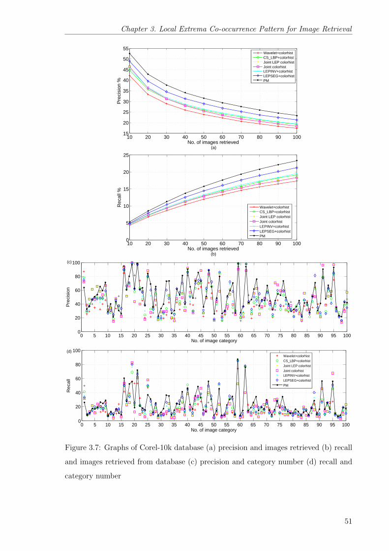
Chapter 3. Local Extrema Co-occurrence Pattern for Image Retrieval
10 20 30 40 50 60 70 80 90 10015
20
25
30
35
40
45
50
55
No. of images retrieved
Pre
cisi
on %
Wavelet+colorhistCS_LBP+colorhistJoint LEP colorhistJoint colorhistLEPINV+colorhistLEPSEG+colorhistPM
(a)
10 20 30 40 50 60 70 80 90 1000
5
10
15
20
25
No. of images retrieved
Rec
all %
Wavelet+colorhistCS_LBP+colorhistJoint LEP colorhistJoint colorhistLEPINV+colorhistLEPSEG+colorhistPM
(b)
0 5 10 15 20 25 30 35 40 45 50 55 60 65 70 75 80 85 90 95 1000
20
40
60
80
100
No. of image category
Pre
cisi
on
(c)
0 5 10 15 20 25 30 35 40 45 50 55 60 65 70 75 80 85 90 95 1000
20
40
60
80
100
No. of image category
Re
call
Wavelet+colorhistCS_LBP+colorhistJoint LEP colorhistJoint colorhistLEPINV+colorhistLEPSEG+colorhistPM
(d)
Figure 3.7: Graphs of Corel-10k database (a) precision and images retrieved (b) recall
and images retrieved from database (c) precision and category number (d) recall and
category number
51

3.4 Experimental results and discussion
SEG+colorhist up to 20.72%, 14.10%, 12.37%, 12.44%, 12.90% and 5.90% respectively.
3.4.3 Experiment 3
Third database in color-natural category is Corel-10k database and the details about
this database are given in Chapter 1, Section 1.2.1.
0 0.1 0.2 0.3 0.4 0.5 0.6 0.7 0.8 0.9 10
0.2
0.4
0.6
0.8
1
Recall
Pre
cisi
on
Wavelet+colorhistCS_LBP+colorhistJoint LEP colorhistJoint colorhistLEPINV+colorhistLEPSEG+colorhistPM
(a)
0 10 20 30 40 50 60 70 80 90 1000
0.05
0.1
0.15
0.2
0.25
Number of top matches
F−m
easu
re
Wavelet+colorhistCS_LBP+colorhistJoint LEP colorhistJoint colorhistLEPINV+colorhistLEPSEG+colorhistPM
(b)
Figure 3.8: (a) Precision-recall curve and (b) F-measure curve for Corel-10k database
Same as previous database, for this database also precision, recall and F-measure
are collected with the help of Eq. [1.6-1.12]. Fig. 3.7 and 3.8 explain the results of
Corel-10k regrading precision, recall and F-measure as compared to other methods, and
table 3.3 indicates that the presented technique outperforms other existing methods.
Precision of the proposed method has been considerably raised from Wavelet+colorhist,
CS LBP+colorhist, Joint LEP colorhist, Joint colorhist, LEPINV+colorhist and LEP-
52

Chapter 3. Local Extrema Co-occurrence Pattern for Image Retrieval
SEG+colorhist up to 20.72%, 14.10%, 12.37%, 12.44%, 12.90% and 5.90% respectively.
3.4.4 Experiment 4
10 20 30 40 50 60 70 80 90 1000
20
40
60
80
100
No. of images retrieved
Pre
cisi
on %
Wavelet+colorhistCS_LBP+colorhistJoint LEP colorhistJoint colorhistLEPINV+colorhistLEPSEG+colorhistPM
(a)
10 20 30 40 50 60 70 80 90 10050
60
70
80
90
100
No. of images retrieved
Rec
all %
Wavelet+colorhistCS_LBP+colorhistJoint LEP colorhistJoint colorhistLEPINV+colorhistLEPSEG+colorhistPM
(b)
Figure 3.9: MIT VisTex database results of (a) average precision and (b) average recall
For color texture image retrieval, MIT VisTex database is used and more explana-
tion about database is given in Chapter 1, Section 1.2.1.
Results of precision, recall and F-measure with number of images retrieved are
demonstrated in Figs. 3.9 and 3.10. Table 3.4 illustrates the results in percentage of
total precision and recall. Retrieval performance is presented as the number of top
matches during experiment for each image in the database. Average retrieval rate of
the proposed method has been increased from Wavelet+colorhist, CS LBP+colorhist,
Joint LEP colorhist, Joint colorhist, LEPINV+colorhist and LEPSEG+colorhist up
53

3.4 Experimental results and discussion
to 22.99%, 14.48%, 12.66%, 12.51%, 15.19% and 16.35% respectively. It is acquired
that the presented method in this work is more advantageous than others in terms of
accuracy.
0 0.1 0.2 0.3 0.4 0.5 0.6 0.7 0.8 0.9 10.75
0.8
0.85
0.9
0.95
1
Recall
Pre
cisi
on
Wavelet+colorhistCS_LBP+colorhistJoint LEP colorhistJoint colorhistLEPINV+colorhistLEPSEG+colorhistPM
(a)
0 2 4 6 8 10 12 14 160
0.2
0.4
0.6
0.8
1
Number of top matches
F−m
easu
re
Wavelet+colorhistCS_LBP+colorhistJoint LEP colorhistJoint colorhistLEPINV+colorhistLEPSEG+colorhistPM
(b)
Figure 3.10: (a) Precision-recall curve and (b) F-measure curve for MIT VisTex
database
3.4.5 Experiment 5
This experiment is conducted on STex database. More information regarding STex
database is presented in Chapter 1, Section 1.2.1. Average precision and recall have
been calculated for all images in the database. In Fig. 3.11, plots of precision and
recall have been presented with number of images retrieved. Precision-recall curve and
54

Chapter 3. Local Extrema Co-occurrence Pattern for Image Retrieval
16 32 48 64 80 96 1120
10
20
30
40
50
60
70
80
No. of images retrieved
Pre
cisi
on
%
Wavelet+colorhistCS_LBP+colorhistJoint LEP colorhistJoint colorhistLEPINV+ColorhistLEPSEG+colorhistPM
(a)
16 32 48 64 80 96 11240
50
60
70
80
90
100
No. of images retrieved
Rec
all %
(b)
Figure 3.11: STex database results of (a) average precision and (b) average recall
F-measure curve have been shown in Fig. 3.12. Average recall rate of the presented
method and other methods have been shown in table 3.4, which clearly show that the
ARR of proposed method is greater than others. Average retrieval rate of the proposed
method has been exceptionally increased from Wavelet+colorhist, CS LBP+colorhist,
Joint LEP colorhist, Joint colorhist, LEPINV+colorhist and LEPSEG+colorhist up to
64.50%, 39.03%, 23.79%, 23.79%, 54.15% and 59.90% respectively.
3.4.6 Experiment results with different distance measure
Four different distance measures, d1, Canberra, Manhattan and Euclidean (Eq. 1.1-
1.4) have been used for measuring the similarity between images. Comparison between
all four distance measures has been shown in table 3.5 for five databases in terms of
55

3.4 Experimental results and discussion
0 0.1 0.2 0.3 0.4 0.5 0.6 0.7 0.8 0.9 10.4
0.5
0.6
0.7
0.8
0.9
1
Recall
Pre
cisi
on
Wavelet+colorhistCS_LBP+colorhistJoint LEP colorhistJoint colorhistLEPINV+colorhistLEPSEG+colorhistPM
(a)
0 2 4 6 8 10 12 14 160.1
0.2
0.3
0.4
0.5
0.6
0.7
0.8
Number of top matches
F−m
easu
re
Wavelet+colorhistCS_LBP+colorhistJoint LEP colorhistJoint colorhistLEPINV+colorhistLEPSEG+colorhistPM
(b)
Figure 3.12: (a) Precision-recall curve and (b) F-measure curve for STex database
average retrieval rate (ARR) and average precision rate (APR). Experiments show that
d1 distance measure is giving better results among others.
3.4.7 Proposed method with different quantization levels
In HSV color space, hue, saturation and value have their own importance. The pro-
posed method is analyzed with different quantization levels of hue and saturation com-
ponents for all the databases in table 3.6. Performance with different quantization
methods differ in different databases, e.g., hue 72 and saturation 20 provide the best
result for Corel 1k database, on the other hand it is not better for other databases.
In the same manner, performance has been observed for other quantization schemes.
56

Chapter 3. Local Extrema Co-occurrence Pattern for Image Retrieval
Table 3.3: Results of Corel-1k, Corel-5k and Corel-10k in precision (for n=10) and
recall (for n=100)
Method Corel-1k Corel-5k Corel-10k
Precision Recall Precision Recall Precision Recall
CS LBP+colorhist 75.88 48.14 54.39 25.47 44.08 18.57
LEPSEG+colorhist 75.80 36.15 43.66 17.62 35.58 13.48
LEPINV+colorhist 72.47 38.56 50.41 20.44 41.25 15.74
Wavelet+colorhist 67.59 40.65 52.15 24.43 42.28 17.34
Joint LEP colorhist 75.13 37.90 53.89 22.85 44.14 16.77
Joint Colorhist 75.15 37.90 53.64 22.71 43.96 16.66
PM 78.58 51.87 62.96 31.16 52.50 23.29
Table 3.4: Average retrieval rate (ARR) for both MIT VisTex and STex database
CS LBP+
colorhist
LEPSEG+
colorhist
LEPINV+
colorhist
Wavelet+
colorhist
Joint LEP
colorhist
Joint
colorhistPM
MIT VisTex 81.23 79.92 80.73 75.61 82.54 82.65 92.99
STEX 53.33 46.37 48.10 45.08 59.90 59.90 74.15
Table 3.5: Experimental results of the proposed method with different distance measure
Corel 1k Corel 5k Corel 10k MIT VisTex STEX
APR ARR APR ARR APR ARR APR ARR APR ARR
d1 78.58 51.87 62.96 31.16 52.50 23.29 92.99 99.22 74.15 90.03
Canberra 75.90 46.77 60.48 27.23 49.84 21.57 91.05 98.76 70.61 87.34
Manhattan 72.86 48.78 52.47 24.62 42.25 18.04 82.80 97.00 65.87 84.95
Euclidean 64.55 41.43 43.61 19.66 34.65 14.32 71.81 92.72 54.18 75.92
Performance of the method depends on the color distribution and the texture of images
present in database.
3.4.8 Computational complexity
Speed of extracting similar images to the query image depends on the feature vector
length of the image. Lengthy feature vector takes more time in calculating the dif-
ference between query image and database images. Comparison of feature vector of
57

3.4 Experimental results and discussion
Table 3.6: Precision and recall of the proposed method with different quantization
schemes for all databases
Corel 1k Corel 5k Corel 10 MIT VisTex STEX
APR ARR APR ARR APR ARR APR ARR APR ARR
HSV(18 10 256) 78.32 50.58 62.96 31.16 52.50 23.29 92.54 99.03 72.63 88.80
HSV(18 20 256) 77.98 51.35 63.10 30.61 52.47 22.93 92.99 99.22 73.25 89.43
HSV(36 10 256) 78.50 50.70 61.56 30.27 51.18 22.60 92.14 99.08 73.37 89.44
HSV(36 20 256) 78.66 51.72 62.89 30.84 52.52 23.05 92.95 99.23 74.15 90.03
HSV(72 10 256) 78.02 50.87 61.23 29.53 51.22 22.13 91.52 99.08 73.32 89.36
HSV(72 20 256) 78.58 51.87 60.46 28.72 50.86 22.21 92.18 99.26 74.01 89.90
Table 3.7: Feature vector (F.V.) length, feature extraction (F.E.) and image retrieval
(I.R.) time of different method
Method F.V. length F.E. time (sec) I.R. time (sec)
CS LBP+colorhist 16+24=40 0.1216 0.51
LEPSEG+colorhist 512+24=536 0.0243 0.59
LEPINV+colorhist 72+24=96 0.0709 0.52
Wavelet+colorhist 24+192=216 0.0757 0.53
Joint LEP colorhist 16× 8× 8× 8 = 8192 0.1676 2.52
Joint colorhist 8× 8× 8 = 512 0.0360 0.58
LECoP(H18S10V256) 18+10+256=284 0.2407 0.54
LECoP(H18S20V256) 18+20+256=294 0.2414 0.54
LECoP(H36S10V256) 36+10+256=302 0.2418 0.54
LECoP(H36S20V256) 36+20+256=312 0.2422 0.55
LECoP(H72S10V256) 71+10+256=338 0.2427 0.56
LECoP(H72S20V256) 72+20+256=348 0.2449 0.56
the proposed method with other methods has been given in table 3.7 for speed evalua-
tion. Also, feature extraction time for one image has been given in table 3.7 for all the
methods including proposed method. For proposed method, feature extraction time
has been mentioned with all quantization levels.
As demonstrated in the table, the feature vector length of the proposed method is
greater than CS LBP+colorhist, LEPINV+colorhist and Wavelet+colorhist, however,
58

Chapter 3. Local Extrema Co-occurrence Pattern for Image Retrieval
it outperforms these methods in terms of accuracy as mentioned in different database
experimental sections. Also, LEPSEG+colorhist, Joint LEP colorhist and Joint col-
orhist have more feature vector length, and take more time than the proposed method
in extracting the similar images to the query image.
3.5 Conclusion
A novel feature descriptor LECoP is proposed for color and texture image retrieval. It
utilizes the properties of local pattern and co-occurrence matrix using the HSV color
space. This method extracts local directional information of each pixel in terms of
LEP, and construct GLCM to obtain the co-occurrence of each pair in LEP map. The
HSV color space is used for color feature. In particular, hue and saturation are used to
extract color and brightness respectively, using histograms. Value component is used
to apply LECoP, and the combined feature vector is applied to benchmark Corel, MIT
VisTex and STex database. The results for the proposed method and previous methods
have been explained using graphs with evaluation measures, and results show that the
proposed method outperforms other methods.
59


Chapter 4
Center Symmetric Local Binary Co-
occurrence Pattern for CBIR
Image feature extraction, according to the user requirement and database images, is
a difficult task in the present scenario. In this chapter, a new image retrieval technique
has been introduced. This technique is useful for different kind of dataset. In the
proposed method, center symmetric local binary pattern (CSLBP) has been extracted
from the original image to obtain the local information. Co-occurrence of pixel pairs
in local pattern map have been observed in different directions and distances using
gray level co-occurrence matrix. Earlier methods have utilized histogram to extract
the frequency information of local pattern map but co-occurrence of pixel pairs is more
robust than frequency of patterns. The proposed method is tested on three different
category of images , i.e., texture, face and medical image database and compared with
some state-of-the-art local patterns.
61

4.1 Preliminaries
4.1 Preliminaries
4.1.1 Center symmetric local binary pattern
0 1 00
8 4 21
0 4 04 0
R=1P=8
98 20 7859 50 5212 88 30
Figure 4.1: Center symmetric local binary pattern computation example
Center symmetric local binary pattern (CSLBP) is proposed by Heikkila [42]. It
extracts a local pattern for every pixel of the input image region. In center symmetric
local binary pattern (CSLBP), a local pattern is extracted from the input image pixels
based on center symmetric pixel difference. Each pixel is considered as center pixel and
difference of center symmetric pixels is calculated which is independent of the center
pixel. Based on the difference, four binary numbers are assigned to the center pixel
that further multiplied by four weights, and summed up to one value, that is called
center symmetric local binary pattern value. A histogram has been created for feature
vector of CSLBP map. CSLBP is explained mathematically in the following equations.
CSLBPP,R,T =
(P/2)−1∑s=0
2s × F3(Is − Is+(P/2)) (4.1)
F3(a) =
1 a > T
0 else
Hist(L) |CSLBP =m∑
x1=1
n∑x2=1
F2(CSLBP(x1, x2), L);L ∈ [0, 15] (4.2)
where T is the threshold parameter and its value is set to 1% of the highest intensity
in the image. Function F2(x, y) is defined as given in Eq. 2.5. An example of CSLBP
is explained in Fig. 4.1. More details about CSLBP can be found in [42].
4.1.2 Gray level co-occurrence matrix
Complete details about gray level co-occurrence matrix (GLCM) are given in Chapter
3, Section 3.1.2.
62

Chapter 4. Center Symmetric Local Binary Co-occurrence Pattern for CBIR
4.2 Proposed method
]1,0[0°
]1,-1[45°[-1,0]90°]-1,-1[135°
]2,0[0°
]2,-2[45°[-2,0]90°]-2,-2[135°
]2,0[0°
]2,-2[45°
]2,0[0°
[-2,0]90°
[-1,0]90°
]1,0[0°]1,0[0°
]1,-1[45°
(a)
(b)
(c) (d)
Figure 4.2: Different combinations of (d, θ) used for feature vector computation in
GLCM
In earlier local patterns, features have been extracted in the form of histograms that
express the frequency of each pattern. Information regarding the mutual occurrence of
patterns was not considered in the histogram. In the proposed method, we have kept
this as an issue and features have been extracted in a improved manner.
In the proposed method, CSLBP has been chosen for local pattern extraction of the
original image. Center symmetric local binary patterns have some important properties
that encouraged us to adopt it as image pattern. The patterns obtained from the
CSLBP are ranged from 0 to 15. Hence, the feature vector length does not exceed
in comparison with the other local patterns. CSLBP considers all neighboring pixels,
and observe the relation between center symmetric pixels. In the proposed method,
63

4.2 Proposed method
CSLBP pattern is extracted from the input image. Closest neighboring ‘8’ pixels with
radius ‘1’, are considered for pattern. It provides a pattern map which is same size as
of the input image. The value of intensity in the pattern map is varying from 0 to 15.
Gray level co-occurrence matrix has been used for feature extraction from the
CSLBP pattern map. The GLCM can be obtained in different directions and with
different distance from the image as explained in section 2.2. In the presented work,
different combinations of distances and angles have been observed and combined ac-
cordingly. Four combinations that have been used, are demonstrated in Fig. 4.2 and
are explained below.
1. In Fig. 4.2(a), four GLCM of distance 1, and angles 0◦, 45◦, 90◦ and 135◦ have
been obtained.
2. In Fig. 4.2(b), four GLCM of distance 2, and angles 0◦, 45◦, 90◦ and 135◦ have
been calculated.
3. Two GLCM of distance 1 with 0◦ and 45◦ directions, and two GLCM of distance
2 with 0◦ and 45◦ directions have been obtained in Fig. 4.2(c).
4. In Fig. 4.2(d), two GLCM of distance 1 with 0◦ and 90◦ angles, and two GLCM
of distance 2 with 0◦ and 90◦ angles have been obtained.
It can be easily seen that all the four above combinations are considering most
adjacent and most close neighboring pixels for GLCM formation. For local analysis,
closest neighboring pixels are more important than far pixels as they reveal more
neighborhood relationship information. Hence, these four combinations have been
used to collect the GLCMs. By using different directions and distances, these all four
combinations gather the pixel pair co-occurrence between most close pixels, and that
is more informative.
Four matrices have been obtained in each of the above methods. All four matrices
have been converted into vectors, and the vectors have been concatenated in single vec-
tor that is called final feature vector. All above four combinations have been observed
in experimental section for performance. The CSLBP pattern map has the intensity of
pixels in a range of [0, 15] (total 16 intensities). Hence, the length of each GLCM ma-
trix is 16× 16, and in the proposed method, four GLCM matrices have been combined
at one time. Final length of feature vector is 4× (16× 16).
64

Chapter 4. Center Symmetric Local Binary Co-occurrence Pattern for CBIR
Mathematically, CSLBCoP can be formulated for an M×N size image as explained
below:
I =M∑x1=1
N∑x2
CSLBP8,1,2.6(x1, x2) (4.3)
GLCMθd(I) = Gθ
d(i, j) ∀ (i, j) ∈ I (4.4)
where I is the CSLBP map of image. Four combinations of GLCM as explained above,
have been used to create four different feature vectors.
FV1(I) = [GLCM0◦
1 GLCM45◦
1 GLCM90◦
1 GLCM135◦
1 ] (4.5)
FV2(I) = [GLCM0◦
2 GLCM45◦
2 GLCM90◦
2 GLCM135◦
2 ] (4.6)
FV3(I) = [GLCM0◦
1 GLCM45◦
1 GLCM0◦
2 GLCM45◦
2 ] (4.7)
FV4(I) = [GLCM0◦
1 GLCM90◦
1 GLCM0◦
2 GLCM90◦
2 ] (4.8)
It has been explained that CSLBP gives a local pattern for each pixel that extracts
the local information of every pixel and transforms whole image into a CSLBP map.
Each CSLBP map contains total 16 intensities. Further, GLCM gives co-occurrence
between pixel pairs in an image. Following reasons influenced us to combine these two
methods:
• CSLBP extracts local information and has significantly less feature vector length.
• Earlier, people used histogram of local pattern map that extracts frequency dis-
tribution but lacks in mutual occurrence of pixel pairs.
• GLCM extracts the spatial information between pixels. Applying GLCM of dif-
ferent direction and distance on CSLBP map makes it possible to extract spatial
information along with frequency distribution from a transformed local map.
An example of feature extraction has been shown in Fig. 4.3. In Fig. 4.3(a) original
image is shown and the CSLBP of original image is calculated in 4.3(b). Gray level co-
occurrence matrices have been obtained and converted into vector form in Fig. 4.3(c).
Finally, joint vector has been shown in Fig. 4.3(d) by concatenating all GLCM vectors.
65

4.3 Proposed system framework
(a) (b)
(c)
(d)
Figure 4.3: Proposed method feature vector computation for sample image
4.3 Proposed system framework
4.3.1 Feature extraction
Figure 4.4: Proposed algorithm block diagram
66

Chapter 4. Center Symmetric Local Binary Co-occurrence Pattern for CBIR
Feature computation has been depicted in the block diagram which is shown in Fig.
4.4. The algorithm for the same is given below.
Input : Image
Output : Feature vector
1. Obtain the gray scale image of the input image.
2. Apply CSLBP and obtain CSLBP map of image.
3. Apply GLCM of ‘1’ distance and 0◦, 45◦, 90◦ and 135◦ directions, and obtain 4
matrices correspond to each direction.
4. Convert all four matrices into vectors, obtained in step 3.
5. Concatenate all four vectors obtained in step 4, into a single feature vector.
4.3.2 Similarity measure
In this chapter, five distances, i.e., d1, Euclidean, Manhattan, Canberra and Chi-square
(Eq. 1.1-1.5) have been used to compute the distance between query and database
image feature vectors. Performance of the proposed method has been observed with
these five distance measures.
4.3.3 Feature matching
Block diagram of the whole system has been shown in Fig. 4.5, and algorithm of the
same has been given below.
Input : Query Image
Output : Retrieved Images
1. Extract the features of query image using proposed algorithm.
2. Compute similarity index between query image feature vector and feature vector
of each database’s image.
3. Sort the similarity index.
4. Retrieve images as final results which correspond to shorter distances.
67

4.4 Experimental results and discussion
Imagedatabase
Featureextraction
Queryimage
Featureextraction
Feature vectorDatabase
SimilarityMeasure
RetrievedImages
Figure 4.5: Block diagram of the proposed system
4.4 Experimental results and discussion
Experiments have been conducted on texture, face and MRI images. In each experi-
ment, precision and recall (Chapter 1 Section 1.2.5) have been calculated and the per-
formance of proposed method is compared with CSLBP [42], LEPINV [168], LEPSEG
[168], DLEP [95], LMEBP [85] and LBP [105]. The proposed method is abbreviated
as CSLBCoP.
4.4.1 Experiment 1
MIT VisTex database (Chapter 1, Section 1.2.1) has been used in first experiment.
Every image of database is used as a query and results are retrieved. For each query,
images are retrieved in groups of 16, 32, 48, .., 112. Average precision and recall have
been shown with number of images retrieved in Fig. 4.6. Precision and recall for other
methods are also calculated in the same manner and plotted in Fig. 4.6. It has been
observed that the proposed method’s average retrieval rate (90.08%) is greater than
CSLBP (79.23%), LEPINV (72.10%), LEPSEG (80.25%), DLEP (80.47%), LMEBP
(87.77%) and LBP (85.84%). Results are also shown in table 4.1. Some query image
examples are shown in Fig. 4.7, where query images are there in first column and
retrieved images from the proposed method are shown next to the query images.
68

Chapter 4. Center Symmetric Local Binary Co-occurrence Pattern for CBIR
16 32 48 64 80 960
20
40
60
80
100
Number of images retrieved
Pre
cisi
on
CSLBPLEPINVLEPSEGLBPLMEBPDLEPCSLBCoP
(b)
16 32 48 64 80 9670
75
80
85
90
95
100
Number of images retrieved
Rec
all
CSLBPLEPINVLEPSEGLBPLMEBPDLEPCSLBCoP
(a)
Figure 4.6: (a) Average precision and (b) recall graph for MIT VisTex database
4.4.2 Experiment 2
In second experiment, Brodatz database (Chapter 1 Section 1.2.1) has been used. For
Brodatz database, retrieved images are grouped in 25, 30, 35,..,70 since each category
holds 25 images. Final results are shown in Fig. 4.8. Graph of precision with number of
image retrieved presented in 4.8(a), and graph of recall with number of image retrieved
is shown in 4.8(b). Average recall rate (ARR) of all methods has been given in table
4.1. Results demonstrated in graphs, clearly indicate that the proposed method is
better than other local patterns, and it is a better texture descriptor.
69

4.4 Experimental results and discussion
Query image Retrieved images
Figure 4.7: Query image retrieval in MIT VisTex texture image database
4.4.3 Experiment 3
In this experiment, ORL face database (Chapter 1, Section 1.2.1) has been utilized.
In ORL face database experiment, images are retrieved in a group of 1, 2, 3,..,10
since the face images are very sensitive and almost similar to each other with minor
changes. Precision and recall graphs are shown in Fig. 4.9(a) and 4.9(b) versus number
of images retrieved. Fig. 4.9 and table 4.1 clearly imply that the proposed method
(64.15%) outperforms others. A query example of face image retrieval is shown in
Fig. 4.10 in which, query images and the corresponding retrieved images are shown.
In Fig. 4.11, a query example for all the methods has been shown. Results can be
seen practically that for the proposed method, all retrieved images belong to the same
category whereas for other methods some false images are retrieved.
4.4.4 Experiment 4
Final experiment in this chapter is conducted on OASIS MRI image database (Chapter
1 Section 1.2.1). For performance measurement, average precision rate (APR) has been
70

Chapter 4. Center Symmetric Local Binary Co-occurrence Pattern for CBIR
25 30 35 40 45 50 55 60 65 7020
30
40
50
60
70
80
Number of images retrieved
Pre
cisi
on
CSLBPLEPINVLEPSEGLBPLMEBPDLEPCSLBCoP
(a)
25 30 35 40 45 50 55 60 65 7055
60
65
70
75
80
85
90
Number of images retrieved
Rec
all
CSLBPLEPINVLEPSEGLBPLMEBPDLEPCSLBCoP
(b)
Figure 4.8: (a) Average precision and (b) recall graph for Brodatz texture database
calculated for each method, including the proposed method. In Fig. 4.12(a), APR with
number of images retrieved has been plotted, and the proposed method outperforms
other methods. Also, group precision for each category has been calculated, and shown
in Fig. 4.12(b). It indicates that the performance of proposed method is much better
for group 2 and group 4 images, and for group 1 and group 3, it is slightly down from few
methods. Average group precision (48.81%) is more satisfactory than other methods
as shown in table 4.1. Query image example of OASIS database is demonstrated in
Fig. 4.13.
71

4.4 Experimental results and discussion
1 2 3 4 5 6 7 8 9 1020
30
40
50
60
70
80
90
100
Number of images retrieved
Pre
cisi
on
CSLBPLEPINVLEPSEGLBPLMEBPDLEPCSLBCoP
(a)
1 2 3 4 5 6 7 8 9 1010
20
30
40
50
60
70
Number of images retrieved
Rec
all
CSLBPLEPINVLEPSEGLBPLMEBPDLEPCSLBCoP
(b)
Figure 4.9: (a) Average precision and (b) recall graph for ORL face database
Table 4.1: Results of previous methods and the proposed method for all databases
MIT VisTex
ARR
Brodatz
ARR
ORL Face
ARR
OASIS MRI
Group Precision
CSLBP 79.23 56.41 54.38 37.98
LEPINV 72.10 56.83 26.63 38.13
LEPSEG 82.23 64.77 37.13 39.15
LBP 85.84 70.06 42.13 42.04
LMEBP 87.77 74.23 46.38 45.69
DLEP 80.47 71.39 51.35 44.80
CSLBCoP 90.08 75.51 64.15 48.81
72
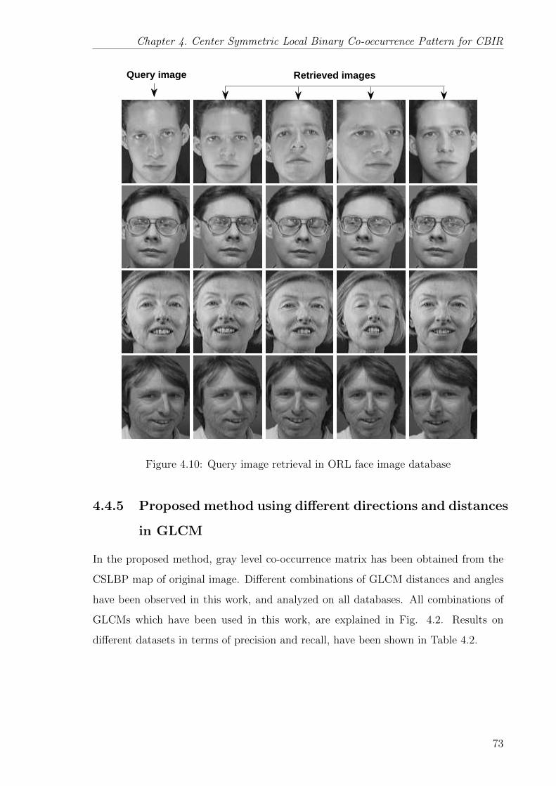
Chapter 4. Center Symmetric Local Binary Co-occurrence Pattern for CBIR
Query image Retrieved images
Figure 4.10: Query image retrieval in ORL face image database
4.4.5 Proposed method using different directions and distances
in GLCM
In the proposed method, gray level co-occurrence matrix has been obtained from the
CSLBP map of original image. Different combinations of GLCM distances and angles
have been observed in this work, and analyzed on all databases. All combinations of
GLCMs which have been used in this work, are explained in Fig. 4.2. Results on
different datasets in terms of precision and recall, have been shown in Table 4.2.
73

4.4 Experimental results and discussion
CSLBP
LEPINV
LEPSEG
LBP
LMEBP
CSLBCoP
DLEP
Figure 4.11: Query image retrieval in ORL face image database for all methods
4.4.6 Proposed system using different distance measure
Similarity index plays a major role in retrieval system. Hence, performance of the
proposed method has been analyzed on five similarity indices as mentioned in section
4.2. All five similarity measures have been explained in Eq. 1.1-1.5. Results for all
databases on different distance measures have been shown in table 4.3. It has been
observed that the results for d1 distance are better from others in all cases. A weight
has been associated with each pattern difference that makes it possible to enhance the
small variation in local patterns. Hence, d1 distance gives better results than others.
Also, in the literature [84, 91, 153], the d1 distance has worked as a better distance
measure for local patterns.
74
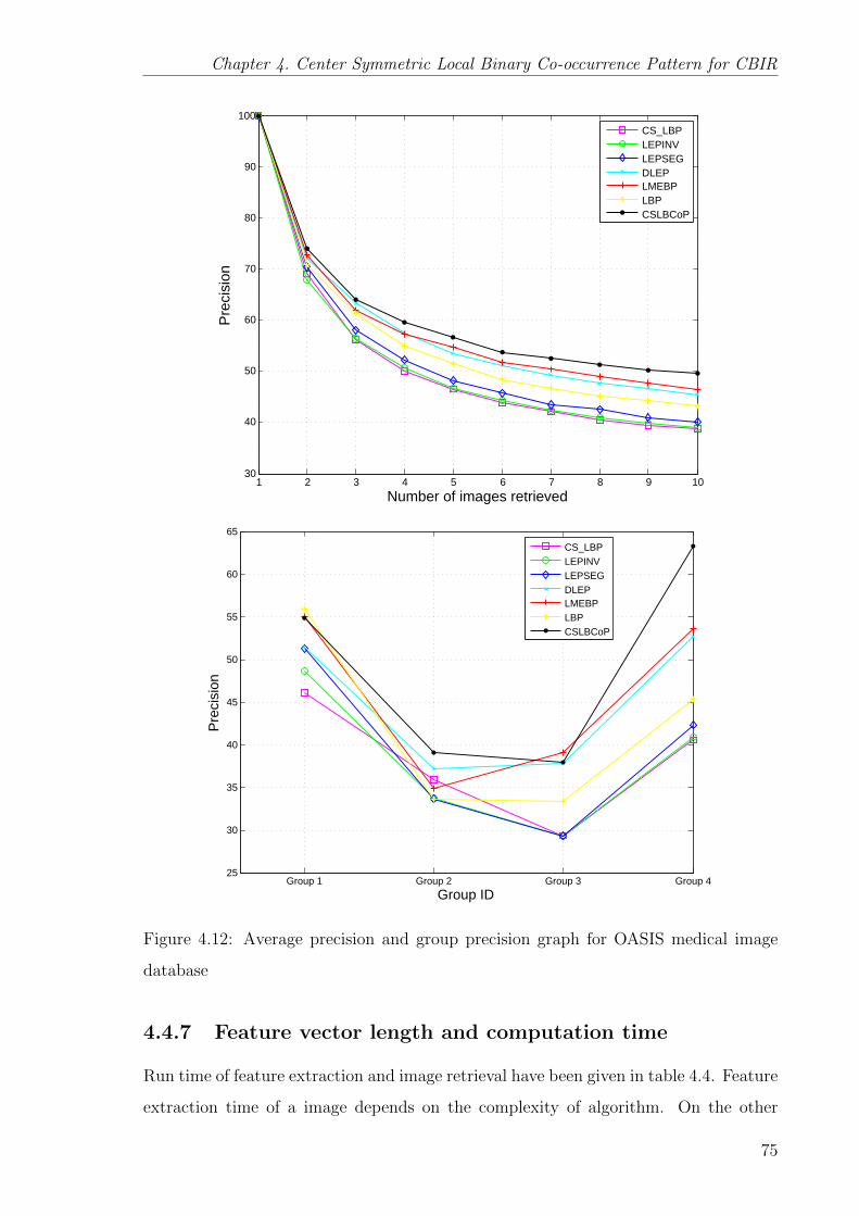
Chapter 4. Center Symmetric Local Binary Co-occurrence Pattern for CBIR
1 2 3 4 5 6 7 8 9 1030
40
50
60
70
80
90
100
Number of images retrieved
Pre
cisi
on
CS_LBPLEPINVLEPSEGDLEPLMEBPLBPCSLBCoP
Group 1 Group 2 Group 3 Group 425
30
35
40
45
50
55
60
65
Group ID
Pre
cisi
on
CS_LBPLEPINVLEPSEGDLEPLMEBPLBPCSLBCoP
1 2 3 4 5 6 7 8 9 1030
40
50
60
70
80
90
100
Number of images retrieved
Pre
cisi
on
CS_LBPLEPINVLEPSEGDLEPLMEBPLBPCSLBCoP
Group 1 Group 2 Group 3 Group 425
30
35
40
45
50
55
60
65
Group ID
Pre
cisi
on
CS_LBPLEPINVLEPSEGDLEPLMEBPLBPCSLBCoP
Figure 4.12: Average precision and group precision graph for OASIS medical image
database
4.4.7 Feature vector length and computation time
Run time of feature extraction and image retrieval have been given in table 4.4. Feature
extraction time of a image depends on the complexity of algorithm. On the other
75

4.4 Experimental results and discussion
Retrieved imagesQuery image
Figure 4.13: Query image retrieval in OASIS medical image database
Table 4.2: Proposed method with different direction and distance in GLCM
MIT VisTex
ARR
Brodatz
ARR
ORL Face
ARR
OASIS MRI
Group Precision
D=1 θ = 0◦, 45◦
D=2 θ = 0◦, 45◦89.85 75.10 62.03 45.59
D=1 θ = 0◦, 90◦
D=2 θ = 0◦, 90◦90.08 75.46 61.68 48.81
D=1
θ = 0◦, 45◦, 90◦, 135◦89.30 74.69 60.63 46.56
D=2
θ = 0◦, 45◦, 90◦, 135◦90.05 75.51 64.15 47.13
hand, image retrieval time hangs on length of feature vector. Feature extraction time
of proposed method is less when compare to all other methods except CSLBP and
LBP. Moreover, accuracy of the proposed method is better than these methods. Image
retrieval time of all the algorithms are approximately equal except DLEP and LMEBP,
as there feature vector length is greater than all other methods. Feature vector length
of all methods is also given in table 4.4.
76

Chapter 4. Center Symmetric Local Binary Co-occurrence Pattern for CBIR
Table 4.3: Results of all databases with different distance metrics
MIT VisTex
ARR
Brodatz
ARR
ORL Face
ARR
OASIS MRI
Group Precision
d1 90.08 75.51 64.15 48.81
Euclidean 81.06 65.77 55.83 42.44
Manhattan 87.14 73.43 61.93 45.08
Canberra 87.34 61.12 55.48 44.12
Chi-square 88.38 74.42 63.20 47.83
Table 4.4: Computation time and feature vector length of all methods
Method F.E. time I.R. time F.V. length
CSLBP 0.0196 0.0322 16
LEPINV 0.0720 0.0323 72
LEPSEG 0.0371 0.0330 512
LBP 0.0192 0.0325 256
LMEBP 0.0900 0.0390 4608
DLEP 0.0380 0.0350 2048
CSLBCoP 0.0320 0.0335 1024
F.E.= Feature extraction, I.R.= Image retrieval, F.V.= Feature vector.
4.5 Conclusion
In this chapter, a new image retrieval method has been developed for multi purpose
image datasets. This method is obtained using powerful center symmetric local binary
pattern and gray level co-occurrence matrix. Local features have been obtained using
CSLBP, and co-occurrence of pixel intensities in CSLBP map has been observed using
GLCM. Gray level co-occurrence matrix of different angles and distances have been
observed and combined as one feature vector. Instead of histogram, GLCM of pattern
map have been proved more robustness in terms of feature descriptor. It gives mutual
occurrence of pixels in different directions that helped in obtaining more vigorous
local information from CSLBP map. This method has been tested on MIT VisTex
77

4.5 Conclusion
texture database, Brodatz texture database, ORL face image database and OASIS MRI
medical image database. Effectiveness of the proposed method has been demonstrated
by experiments and proved by comparing other local patterns.
78

Chapter 5
Local Tri-Directional Patterns : A
New Feature Descriptor
In image retrieval, local features extract the information regarding local objects in
the image or local intensity of pixels. Local patterns consider the neighboring pixels
to extract the local information in the image. Most of the local patterns proposed
by researchers, were uniform for all neighboring pixels. A very few patterns utilized
the pixel information based on the direction. The main objective of this work is to
develop a direction based local pattern which can provide better features with respect
to uniform local patterns.
In this chapter, a new texture feature descriptor has been developed which is using
local intensity of pixels based on three directions in the neighborhood and named as the
local tri-directional patterns (LTriDPs). Further, a magnitude pattern is merged for
better feature extraction. The proposed method has been tested on three databases, in
which first two, Brodatz texture image database and MIT VisTex database are texture
image databases and third one is the ORL face database. Further, the effectiveness
of the proposed method is proven by comparing it with existing algorithms for image
retrieval application.
79

5.1 Preliminaries
5.1 Preliminaries
5.1.1 Local binary pattern
3 7 18 6 85 2 9
0 1 01 10 0 1
8 4 216 132 64 128
0 4 016 149 10 0 128
Figure 5.1: Local binary pattern example
Local binary patterns (LBPs) have been proposed by Ojala et al. for local informa-
tion of pixels in an image. In this method, all pixels of the image have been considered
as center pixel, and local information extracted for each pixel that depends on neigh-
boring pixels. Each center pixel is subtracted from all neighboring pixels, and a binary
number is assigned to each neighboring pixel that depends on the difference of center
pixel and neighboring pixel. These binary numbers construct the local binary pattern
for each center pixel. Further, local binary patterns multiplied by some weights and
summed up to a pattern value that is called local binary pattern value for a center pixel.
For a center pixel Ic and neighboring pixels In (n=1,2,..,8), LBP can be computed as
follows:
LBPP,R =P−1∑n=0
2n × F4(In − Ic) (5.1)
F4(x) =
1 x ≥ 0
0 else
where P and R are the number of neighboring pixels and radius respectively. Histogram
of LBP map has been calculated using Eq. 5.2, where m× n is the size of image and
F2(x, y) is defined as given in Eq. 2.5. A sample window example of LBP pattern is
shown in Fig. 5.1.
Hist(L)∣∣LBP
=m∑a=1
n∑b=1
F2(LBP (a, b), L);
L ∈ [0, (2P − 1)]
(5.2)
80

Chapter 5. Local Tri-Directional Patterns : A New Feature Descriptor
5.2 Proposed method
3 7 18 6 85 2 9
3 7 18 6 85 2 9
I6 I7 I8
I5 Ic I1
I4 I3 I2
3 7 18 6 85 2 9
3 7 18 6 85 2 9
3 7 18 6 85 2 9
3 7 18 6 85 2 9
3 7 18 6 85 2 9
3 7 18 6 85 2 9
3 7 18 6 85 2 9
101 1 111 0 000 0 100 2
111 0 000 0 111 0 000 0
Tri-directional pattern = 10020000
01.78)-(98)-(18.56)-(96)-(1
22
22→
=+
=+ 06.72)-(52)-(92.36)-(56)-(9
22
22→
=+
=+ 12.45)-(85)-(25.46)-(86)-(2
22
22→
=+
=+01.79)-(29)-(85.46)-(26)-(8
22
22→
=+
=+
08.58)-(38)-(52.36)-(36)-(5
22
22→
=+
=+ 02.77)-(17)-(38.56)-(16)-(3
22
22→
=+
=+ 02.91)-(81)-(72.26)-(86)-(7
22
22→
=+
=+04.63)-(73)-(82.26)-(76)-(8
22
22→
=+
=+
Magnitude pattern = 0001000010000000 00010000
(a) (b)
(c) (d) (e) (f)
(i) (j)(g) (h)
Figure 5.2: Sample window example of the proposed method
Local tri-directional pattern is an extension of LBP. Instead of uniform relation-
ship with all neighboring pixels, LTriDP considers the relationship based on different
directions. Each center pixel have some neighboring pixels in a particular radius.
Closest neighbor consists of 8 pixels all around the center pixel. Further, there are
16 pixels in next radius and so on. Closest neighboring pixels are less in number
and gives more related information as they are nearest to center pixel. Hence, we
consider 8-neighborhood pixels for pattern creation. Each neighborhood pixel at one
time is considered and compared it with center pixel and also with two most adjacent
neighborhood pixels. These two neighborhood pixels are either vertical or horizontal
81
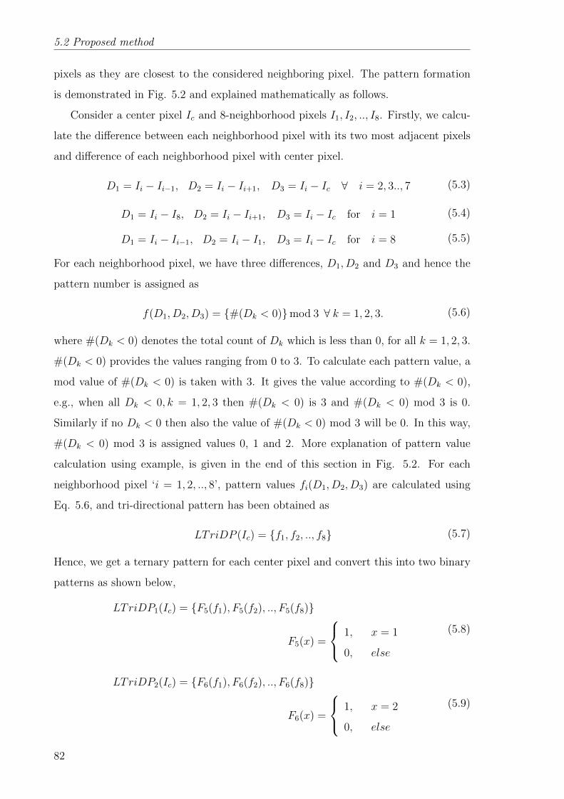
5.2 Proposed method
pixels as they are closest to the considered neighboring pixel. The pattern formation
is demonstrated in Fig. 5.2 and explained mathematically as follows.
Consider a center pixel Ic and 8-neighborhood pixels I1, I2, .., I8. Firstly, we calcu-
late the difference between each neighborhood pixel with its two most adjacent pixels
and difference of each neighborhood pixel with center pixel.
D1 = Ii − Ii−1, D2 = Ii − Ii+1, D3 = Ii − Ic ∀ i = 2, 3.., 7 (5.3)
D1 = Ii − I8, D2 = Ii − Ii+1, D3 = Ii − Ic for i = 1 (5.4)
D1 = Ii − Ii−1, D2 = Ii − I1, D3 = Ii − Ic for i = 8 (5.5)
For each neighborhood pixel, we have three differences, D1, D2 and D3 and hence the
pattern number is assigned as
f(D1, D2, D3) = {#(Dk < 0)}mod 3 ∀ k = 1, 2, 3. (5.6)
where #(Dk < 0) denotes the total count of Dk which is less than 0, for all k = 1, 2, 3.
#(Dk < 0) provides the values ranging from 0 to 3. To calculate each pattern value, a
mod value of #(Dk < 0) is taken with 3. It gives the value according to #(Dk < 0),
e.g., when all Dk < 0, k = 1, 2, 3 then #(Dk < 0) is 3 and #(Dk < 0) mod 3 is 0.
Similarly if no Dk < 0 then also the value of #(Dk < 0) mod 3 will be 0. In this way,
#(Dk < 0) mod 3 is assigned values 0, 1 and 2. More explanation of pattern value
calculation using example, is given in the end of this section in Fig. 5.2. For each
neighborhood pixel ‘i = 1, 2, .., 8’, pattern values fi(D1, D2, D3) are calculated using
Eq. 5.6, and tri-directional pattern has been obtained as
LTriDP (Ic) = {f1, f2, .., f8} (5.7)
Hence, we get a ternary pattern for each center pixel and convert this into two binary
patterns as shown below,
LTriDP1(Ic) = {F5(f1), F5(f2), .., F5(f8)}
F5(x) =
1, x = 1
0, else
(5.8)
LTriDP2(Ic) = {F6(f1), F6(f2), .., F6(f8)}
F6(x) =
1, x = 2
0, else
(5.9)
82

Chapter 5. Local Tri-Directional Patterns : A New Feature Descriptor
LTriDP (Ic)∣∣i=1,2
=7∑l=0
2l × LTriDPi(Ic)(l + 1) (5.10)
After getting pattern map, the histogram is calculated for both binary patterns using
Eq. 5.11, where Pattren is LTriDP |i (i=1,2).
Hist(L)∣∣Pattern
=m∑a=1
n∑b=1
F2(Pattern(a, b), L);
L ∈ [0, 255]
(5.11)
The tri-direction pattern is extracting most of the local information, however it has
been shown that the magnitude pattern is also helpful in creation of more informative
feature vector [38, 96]. We have also employed a magnitude pattern based on center
pixel, neighborhood pixel and two most adjacent pixels. Magnitude pattern is created
as follows:
M1 =√
(Ii−1 − Ic)2 + (Ii+1 − Ic)2
M2 =√
(Ii−1 − Ii)2 + (Ii+1 − Ii)2 ,∀ i = 2, 3.., 7(5.12)
M1 =√
(I8 − Ic)2 + (Ii+1 − Ic)2
M2 =√
(I8 − Ii)2 + (Ii+1 − Ii)2, for i = 1(5.13)
M1 =√
(Ii−1 − Ic)2 + (I1 − Ic)2
M2 =√
(Ii−1 − Ii)2 + (I1 − Ii)2, for i = 8(5.14)
Values of M1 and M2 are calculated for each neighborhood pixel and according to these
values, a magnitude pattern value is assigned to each neighborhood pixel.
Magi(M1,M2) =
1, M1 ≥M2
0, else(5.15)
LTriDPmag(Ic) = {Mag1,Mag2, ..,Mag8} (5.16)
LTriDP (Ic)∣∣mag
=7∑l=0
2l × LTriDPmag(Ic) (5.17)
Similarly, the histogram of the magnitude pattern is created by Eq. 5.11, where
Pattern is LTriDP |mag, and three histograms are concatenated as one.
Hist = [Hist∣∣LTriDP1
, Hist∣∣LTriDP2
, Hist∣∣LTriDPmag
] (5.18)
An example of pattern calculation is shown in Fig. 5.2 through (a)-(j) windows. In
window (a), center pixel Ic and neighborhood pixels I1, I2, .., I8 are shown. Center pixel
83

5.2 Proposed method
is marked as red color in windows (b)-(j). In the next window (c), first neighborhood
pixel I1 is marked as blue color, and two most adjacent pixels marked as yellow color.
First, we compare blue pixel with yellow pixels and red pixel, and assign ‘0’ or ‘1’
value for all the three comparisons. For example, in window (c) I1 is compared with
I8, I2 and Ic. Since I1 > I8, I1 < I2 and I1 > Ic, the pattern for I1 is 101. Now,
according to Eq. 5.6 the pattern value for I1 is 1. In the same way, for next windows
(d)-(j) pattern values are obtained for other neighboring pixels. Finally, the local
tri-directional pattern for center pixel is obtained by merging all neighborhood pixel
pattern values. For magnitude pattern, magnitude of center pixel and neighborhood
pixel is obtained and compared. In the presented example, ‘6’ is center pixel and
I1 is ‘8’. In window (c), magnitude of the center pixel ‘6’ is 5.8 and magnitude of
‘8’ is 7.1 with respect to ‘1’ and ‘9’. Since, the magnitude of center pixel is less than
neighborhood pixel, we assign ‘0’ pattern value here. Consequently, magnitude pattern
is calculated for next neighborhood pixels and shown in (d)-(j) windows, and magnitude
patterns of all neighborhood pixels are merged into one pattern, and that is magnitude
pattern for center pixel. Boundary pixels in each image have been left and LTriDP is
calculated for all pixels except boundary pixels.
Local patterns use local intensity of pixels for grabbing the information and create
the pattern according to the information. Local binary patterns compare the neighbor-
hood pixel and center pixel and assign a pattern to the center pixel. In the proposed
work, additional relationships among local pixels have been observed. Along with re-
lationship of center-neighborhood pixels, mutual relationship of adjacent neighboring
pixels are obtained, and local information based on three direction pixels are exam-
ined. This method gives more information compare to LBP and other local patterns, as
it calculates center-neighboring pixel information alongwith mutual neighboring pixel
information. Nearest neighbors gives most of the information. Hence, the pattern
is calculated using most adjacent neighboring pixels for each pattern value. Also, a
magnitude pattern is introduced which provides information regarding intensity weight
for each pixel. Both LTriDP and magnitude pattern, give different information and
concatenation provides better feature descriptor.
84

Chapter 5. Local Tri-Directional Patterns : A New Feature Descriptor
5.3 Proposed system framework
A block diagram of the presented method is shown in Fig. 5.3, and algorithm for the
same is demonstrated below. Two parts of the algorithm are given in Section 5.3.1. In
part 1, feature vector construction is explained, and in part 2, image retrieval system
is presented.
5.3.1 Algorithm
Part 1: Feature vector construction
Input: Image.
Output: Feature vector.
1. Upload the image and convert it into gray scale if it is a color image.
2. Compute the tri-directional patterns and construct histogram.
3. Evaluate the magnitude patterns and make histogram.
4. Concatenate both the histograms calculated in step 2 and step 3.
Part 2: Image retrieval
Input: Query image.
Output: Similar images to the query.
1. Enter the query image.
2. Calculate the feature vector as shown in part 1.
3. Compute the similarity index of query image feature vector with every database
image feature vector.
4. Sort similarity indices and produce images corresponding to minimum similarity
indices as results.
5.3.2 Similarity measure
Similarity of query image and database image has been measured using d1 distance
measure (Eq. 1.1).
85

5.4 Experimental results and discussion
QueryImage
Tri-directionalpattern
Queryfeaturevector Similarity
match
Imagesretrieved
ImageDatabase
Feature vectordatabase
Magnitudepattern
Histogram3
Histogram1
Jointhistogram
Histogram2
Figure 5.3: Block diagram of the proposed method
5.4 Experimental results and discussion
The proposed method has been tested on two texture database and one face image
database for validation. The capability of the presented method for image retrieval is
shown on the basis of precision, recall [82] and average normalized modified retrieval
rank (ANMRR) [77]. Precision, recall and ANMRR are explained in Chapter 1, Section
1.2.5. In the process of retrieving images, for a given query, many images are retrieved.
In those images, some are relevant to query image and some are non-relevant results
which do not match query image. Every image of the database is treated as a query
image, and for each image, precision, recall and normalized modified retrieval rank
(NMRR) are calculated. The proposed method is compared with CS LBP, LEPINV,
LEPSEG, LBP, LMEBP and DLEP in the following experiments.
5.4.1 Experiment 1
In the first experiment, MIT VixTex database [3] of gray scale images is used and the
details of this database are given in Chapter 1, Section 1.2.1.
Precision and recall for the presented method and other methods are calculated
and demonstrated through graphs. In Fig. 5.4, plots of precision and recall are shown.
86

Chapter 5. Local Tri-Directional Patterns : A New Feature Descriptor
16 32 48 64 80 9610
20
30
40
50
60
70
80
90
No. of images retrieved
Prec
isio
n
CS_LBPLEPINVLEPSEGLBPLMEBPDLEPPM
(b)
16 32 48 64 80 9670
75
80
85
90
95
100
No. of images retrieved
Rec
all
CS_LBPLEPINVLEPSEGLBPLMEBPDLEPPM
(a)
Figure 5.4: Precision and recall with number of images retrieved for database 1
Table 5.1: Average retrieval rate of all databases
Method Brodatz Database MIT VisTex Database ORL Face Database
CS LBP 54.74 74.39 44.35
LEPINV 56.83 72.10 26.63
LEPSEG 64.76 80.25 37.13
LBP 70.06 82.27 42.13
LMEBP 74.23 87.77 46.38
DLEP 71.39 80.47 51.35
PM 76.45 88.62 55.10
87

5.4 Experimental results and discussion
16 32 48 64 80 9610
20
30
40
50
60
70
80
90
97
No. of images retrieved
Prec
isio
n
16 32 48 64 80 96
86
88
90
92
94
96
98
No. of images retrieved
Rec
all
LTriDPLTriDP
mag
(b)(a)
16 32 48 64 80 9610
20
30
40
50
60
70
80
90
97
No. of images retrieved
Prec
isio
n
16 32 48 64 80 96
86
88
90
92
94
96
98
No. of images retrieved
Rec
all
LTriDPLTriDP
mag
(b)(a)
Figure 5.5: (a) Precision and (b) recall of proposed methods for database 1
88
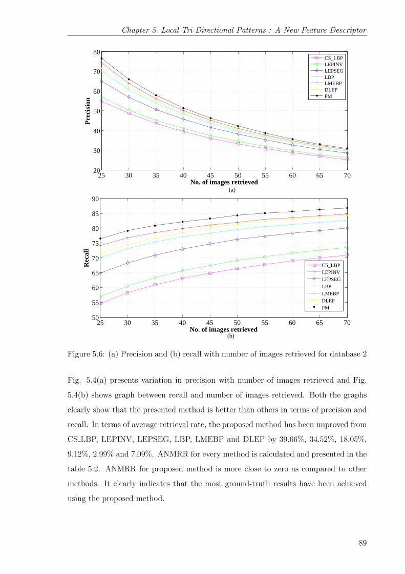
Chapter 5. Local Tri-Directional Patterns : A New Feature Descriptor
25 30 35 40 45 50 55 60 65 7020
30
40
50
60
70
80
No. of images retrieved
Pre
cisi
on
CS_LBPLEPINVLEPSEGLBPLMEBPDLEPPM
(a)
25 30 35 40 45 50 55 60 65 7050
55
60
65
70
75
80
85
90
No. of images retrieved
Rec
all
CS_LBPLEPINVLEPSEGLBPLMEBPDLEPPM
(b)
Figure 5.6: (a) Precision and (b) recall with number of images retrieved for database 2
Fig. 5.4(a) presents variation in precision with number of images retrieved and Fig.
5.4(b) shows graph between recall and number of images retrieved. Both the graphs
clearly show that the presented method is better than others in terms of precision and
recall. In terms of average retrieval rate, the proposed method has been improved from
CS LBP, LEPINV, LEPSEG, LBP, LMEBP and DLEP by 39.66%, 34.52%, 18.05%,
9.12%, 2.99% and 7.09%. ANMRR for every method is calculated and presented in the
table 5.2. ANMRR for proposed method is more close to zero as compared to other
methods. It clearly indicates that the most ground-truth results have been achieved
using the proposed method.
89

5.4 Experimental results and discussion
20 25 30 35 40 45 50 55 60 65 70 7525
30
35
40
45
50
55
60
65
70
75
80
No. of images retrieved
Prei
sion
LTriDPLTriDP
mag
20 25 30 35 40 45 50 55 60 65 70 7570
72
74
76
78
80
82
84
86
88
No. of images retrieved
Rec
all
LTriDPLTriDP
mag
(b)(a)
20 25 30 35 40 45 50 55 60 65 70 7525
30
35
40
45
50
55
60
65
70
75
80
No. of images retrieved
Prei
sion
LTriDPLTriDP
mag
20 25 30 35 40 45 50 55 60 65 70 7570
72
74
76
78
80
82
84
86
88
No. of images retrieved
Rec
all
LTriDPLTriDP
mag
(b)(a)
Figure 5.7: (a) Precision and (b) recall of the proposed methods for database 2
In addition, we have shown the comparison of the proposed methods mutually. In
Fig. 5.5, comparison of LTriDP and LTriDPmag has been shown in terms of precision
and recall with the number of images retrieved. It is clearly visible, that the LTriDP
is more precise than LTriDPmag.
90

Chapter 5. Local Tri-Directional Patterns : A New Feature Descriptor
5.4.2 Experiment 2
1 2 3 4 5 6 7 8 9 1020
30
40
50
60
70
80
90
100
Number of images retrieved
Prec
isio
n
CS_LBPLEPINVLEPSEGLBPLMEBPDLEPPM
(a)
1 2 3 4 5 6 7 8 9 10
10
20
30
40
50
60
Number of images retrievd
Rec
all
CS_LBPLEPINVLEPSEGLBPLMEBPDLEPPM
(b)
Figure 5.8: (a) Precision and (b) recall with number of images retrieved for database 3
In the second experiment, Brodatz textures [127] have been used for testing. Details
about Brodatz database are given in Chapter 1, Section 1.2.1.
The results of the proposed algorithm in the form of precision and recall are pre-
sented in graphs. In this system, initially 25 images are retrieved for each query, and
then an increment of 5 has been applied, and up to 70 images are retrieved. Plots
of precision and recall with number of retrieved images are shown in Fig. 5.6. The
proposed method is more satisfying than other methods and it is clearly visible in
the graphs. Moreover, result of ANMRR are shown in table 5.2, and it implies that
more relevant images are retrieved using the proposed method as compared to other
91

5.4 Experimental results and discussion
Table 5.2: Average normalized modified retrieval rank of different methods and
databases
Method Brodatz Database MIT VisTex Database ORL Face Database
CS LBP 0.3664 0.1696 0.4607
LEPINV 0.3437 0.1876 0.6638
LEPSEG 0.2704 0.1198 0.5398
LBP 0.2278 0.0817 0.4833
LMEBP 0.1944 0.0738 0.4422
DLEP 0.1685 0.1278 0.3918
PM 0.1742 0.0679 0.3570
methods. Fig. 5.7 shows the plots between LTriDP and LTriDPmag. On the basis of
precision and recall, LTriDP is more effective than LTriDPmag, however combination of
both has enhanced the image information as shown in Fig. 5.6.
5.4.3 Experiment 3
In the third experiment, ORL face database [5] has been taken for face image retrieval
purpose. Results of database 3 have been presented in Figs. 5.8 and 5.9. In image
retrieval experimental setup, images have been retrieved in a group of 1, 2, .., 10 images,
and precision and recall have been calculated for each group and shown in Fig. 5.8. The
performance measures in experimental results clearly depict that the proposed method
(55.10%) outperforms DLEP (51.35%), LMEBP (46.38%), LBP (42.13%), LEPSEG
(37.13%), LEPINV (26.63%) and CS LBP (44.35%). Average normalized modified
retrieval rank for this database is shown in table 5.2. For the proposed method it is
more close to zero as compared to other methods, hence the proposed method is more
promising than others in terms of accurate retrieval. Further, in Fig. 5.9, comparison
between LTriDP and LTriDPmag is shown.
Feature vector length of each method is shown in table 5.3. Feature vector length
of the proposed method is comparatively very less from LMEBP and DLEP, and per-
formance is better. Feature vector length of the proposed method is more than CS LBP,
92

Chapter 5. Local Tri-Directional Patterns : A New Feature Descriptor
0 1 2 3 4 5 6 7 8 9 10 11
50
60
70
80
90
100
No. of images retrieved
Prec
isio
n
0 1 2 3 4 5 6 7 8 9 10 115
10
15
20
25
30
35
40
45
50
55
60
No. of images retrieved
Rec
all
LTriDPLTriDP
mag
LTriDPLTriDP
mag
(a) (b)
0 1 2 3 4 5 6 7 8 9 10 11
50
60
70
80
90
100
No. of images retrieved
Prec
isio
n
0 1 2 3 4 5 6 7 8 9 10 115
10
15
20
25
30
35
40
45
50
55
60
No. of images retrieved
Rec
all
LTriDPLTriDP
mag
LTriDPLTriDP
mag
(a) (b)
Figure 5.9: (a) Precision and (b) recall of proposed methods for database 3
LEPINV, LEPSEG and LBP, but performance is considerably better as shown in dif-
ferent database results.
93

5.4 Experimental results and discussion
Query image Retrieved images
Figure 5.10: ORL database query example
Demonstration of the proposed method is shown in Fig. 5.10. Similar face images
have been retrieved for five query images. In Fig. 5.10, first image in each row is
query image and next three images are retrieved images using the proposed method.
Table 5.1 explains the average retrieval rate (ARR) of two texture databases and one
face image database for all compared methods with the proposed method. Final ARR
results clearly verify that the proposed algorithm outperforms others.
94

Chapter 5. Local Tri-Directional Patterns : A New Feature Descriptor
Table 5.3: Feature vector length of different methods
Method Feature vector length
CS LBP 16
LEPINV 72
LEPSEG 512
LBP 256
LMEBP 4096
DLEP 2048
PM 768
5.5 Conclusion
A novel method, named as Local tri-directional pattern, has been proposed in this
chapter and abbreviated as LTriDP. Each pixel in the neighborhood has been compared
with the most adjacent pixels and center pixel for local information extraction. In most
of the previous local patterns, only center pixel is considered for pattern formation,
however in the proposed method, information related to each pixel of neighborhood
is extracted, therefore, this method is giving more enhanced features. The magnitude
pattern is also incorporated, that is again based on the same pixels used in LTriDP.
All methods are tested on MIT VisTex texture database, Brodatz texture database
and ORL face image database. Precision and recall show that the proposed system
more proficient and appropriate than others in terms of accuracy. Further, the feature
vector length of the proposed algorithm is more acceptable than LMEBP and DLEP.
95


Chapter 6
Local Neighborhood Difference Pat-
tern : A New Feature Descriptor
A new image retrieval technique called local neighborhood difference pattern (LNDP)
has been proposed for local features. The conventional local binary pattern (LBP)
transforms every pixel of image into a binary pattern based on their relationship with
neighboring pixels. The proposed feature descriptor differs from local binary pattern as
it transforms the mutual relationship of all neighboring pixels in a binary pattern. Both
LBP and LNDP are complementary to each other as they extract different information
using local pixel intensity.
In the proposed method, both LBP and LNDP features are combined to extract
extreme information. To prove the excellence of the proposed method, two experiments
have been conducted on four different database of texture images and natural images.
The performance has been observed using well-known evaluation measures, precision
and recall, and compared with some state-of-art local patterns. Comparison shows a
significant improvement in the proposed method over existing methods.
97

6.1 Preliminaries
6.1 Preliminaries
6.1.1 Local binary pattern
The complete details of local binary pattern is given in Chapter 5, Section 5.1.1.
6.1.2 Local ternary pattern
2 5 38 5 29 1 7
-1 0 0+1 -1+1 -1 0
8 4 216 132 64 128
0 0 016 48 032 0 0
(a) (b) (c)
(d) (e)
-3 0 -23 -34 -4 2
0 0 01 01 0 0
1 0 00 10 1 0
8 4 216 132 64 128
8 0 00 73 10 64 0
(f)
Figure 6.1: Local ternary pattern calculation (a) a window example (b) difference of
neighboring and center pixel (c) ternary pattern for t=3 (d) ternary pattern divided in
two binary patterns (e) weights (f) weights multiplied by binary patterns and sum up
to pattern value
Local ternary pattern (LTP) is an extension of LBP for noisy images. In this local
pattern, threshold of neighboring and center pixel is processed by an interval instead
of single value. LTP can be explained mathematically as follows:
LTPp,r,t =
p−1∑n=0
2n × F7(In − Ic, t) (6.1)
F7(x, t) =
+1 if x ≥ t
−1 if x ≤ −t
0 if− t < x < t
(6.2)
where p, r and t are number of neighboring pixels, radius and threshold interval value
respectively. Parameter t depends on the maximum number of intensity and noise
98
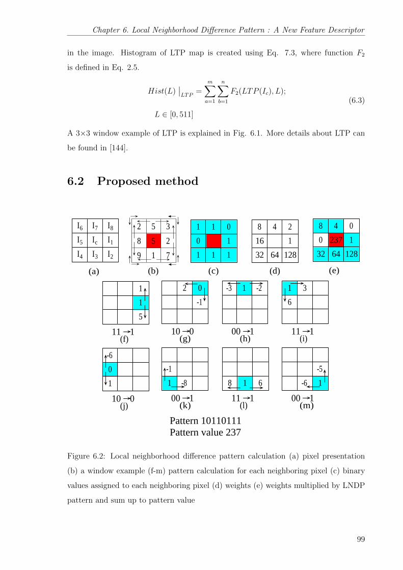
Chapter 6. Local Neighborhood Difference Pattern : A New Feature Descriptor
in the image. Histogram of LTP map is created using Eq. 7.3, where function F2
is defined in Eq. 2.5.
Hist(L)∣∣LTP
=m∑a=1
n∑b=1
F2(LTP (Ic), L);
L ∈ [0, 511]
(6.3)
A 3×3 window example of LTP is explained in Fig. 6.1. More details about LTP can
be found in [144].
6.2 Proposed method
I6 I7 I8I5 Ic I1I4 I3 I2
11 1
115
(f) 10 0
2 0-1
(g) 00 1
-3 1 -2
(h) 11 1
1 36
(i)
10 0
-601
(j) 00 1
-11 -8
(k) 11 18 1 6
(l) 00 1
-5-6 1
(m)
1 1 00 11 1 1
8 4 216 132 64 128
2 5 38 5 29 1 7
8 4 00 237 1
32 64 128(a) (b) (c) (d) (e)
Pattern 10110111Pattern value 237
Figure 6.2: Local neighborhood difference pattern calculation (a) pixel presentation
(b) a window example (f-m) pattern calculation for each neighboring pixel (c) binary
values assigned to each neighboring pixel (d) weights (e) weights multiplied by LNDP
pattern and sum up to pattern value
99

6.2 Proposed method
A new feature extraction method called local neighborhood difference pattern (LNDP),
has been proposed in this chapter. As it appears from the name, this method extracts
the local features based on neighborhood pixel differences, and form a binary pattern
to represent each pixel in the image. For each pixel, 8 neighboring pixels have been
considered, and for each neighboring pixel again two most appropriate pixels are cho-
sen. Relationship of these two pixels have been obtained with neighboring pixel, and a
binary number is assigned. Similarly, for each neighboring pixel a binary number is ob-
tained. Pattern of these binary numbers is formed to represent each pixel, and finally,
histogram is constructed to represent the image in the form of LNDP. For neighboring
pixels In (n=1, 2, .., 8) of a center pixel Ic, LNDP can be computed in the following
procedure:
kn1 = I8 − In, kn2 = In+1 − In, for n = 1 (6.4)
kn1 = In−1 − In, kn2 = In+1 − In, ∀ n = 2, 3, .., 7 (6.5)
kn1 = In−1 − In, kn2 = I1 − In, for n = 8 (6.6)
Difference of each neighborhood pixel with two other neighborhood pixels have been
obtained in kn1 and kn2 . Based on these two differences, a binary number is assigned to
each neighboring pixel.
F1(kn1 , k
n2 ) =
1 kn1 × kn2 ≥ 0
0 else(6.7)
For the center pixel Ic, LNDP can be computed using above binary values as follows:
LNDP (Ic) =8∑
n=1
2n−1 × F1(kn1 , k
n2 ) (6.8)
Histogram for LNDP map can be achieved as follows:
Hist(L) |LNDP =m∑x=1
n∑y=1
F2(LNDP(x, y), L);
L ∈ [0, (28 − 1)]
In Fig. 6.2, an example of LNDP calculation has been demonstrated. In window (a)
and (b), numbering of neighborhood pixels and intensities have been shown. In window
(f)-(m), pattern calculation has been presented. For example, in window (f), pixel I1
has been considered, and differences of I1 with I8 and I2 are obtained using Eq. 7.4,
100

Chapter 6. Local Neighborhood Difference Pattern : A New Feature Descriptor
and those are ‘1’ and ‘5’ respectively. Since both the differences are positive, ‘1’ pattern
value is assigned to I1 pixel (using Eq. 6.7). Similarly, for other pixels, pattern values
have been obtained, and shown in window (c). Pattern values are multiplied by weights
as shown in window (d), and LNDP are obtained by summation of pattern values in
window (e).
6.3 Proposed system framework
6.3.1 Feature extraction
(a) (b)
(c)
Figure 6.3: (a) LBP features (b) LNDP features (c) Concatenation of LBP and LNDP
In the proposed system, features have been extracted using local intensities from
the closest neighborhood of a center pixel. Earlier LBP [105] and the proposed LNDP,
both extract the local features. LBP is based on center-neighboring pixel relationship.
Alternatively, LNDP operator extracts the relationship among neighboring pixels itself.
Both the operators are complement to each other. Hence, in the proposed work, both
operators are employed to achieve the most of the information (Fig. 6.3). For both
LBP and LNDP, pattern map is extracted using each pixel of image except boundary
pixels. Histogram of LBP and LNDP are concatenated for final feature vector for each
image.
101

6.4 Experimental results and discussion
6.3.2 Algorithm
Queryimage
Localneighborhood
differencepattern
Queryfeaturevector
Similaritymatch
ImagesretrievedImage
database
Feature vectordatabase
Local binarypattern Histogram 2
Jointhistogram
Histogram 1
Figure 6.4: Block diagram of the proposed system
Block diagram of the presented method has been demonstrated in Fig. 6.4 and
algorithm for the same is given below:
1. Upload the image, and convert it into a gray scale image if it is a color image.
2. Compute local binary pattern of the image.
3. Compute local neighborhood difference pattern of the image.
4. Create histograms of LBP and LNDP maps.
5. Concatenate both histograms as feature descriptor.
6. Compute the distance of the query image feature vector with all database image
feature vectors using Eq. 1.1.
7. Sort the distances, and produce a set of images with least distances as similar
image results.
102

Chapter 6. Local Neighborhood Difference Pattern : A New Feature Descriptor
25 30 35 40 45 50 55 60 65 7020
30
40
50
60
70
80
Number of images retrieved
Pre
cisi
on
CSLBPLEPINVLEPSEGLBPDLEPLTrPPM
(a)
25 30 35 40 45 50 55 60 65 7055
60
65
70
75
80
85
90
Number of images retrieved
Rec
all
CSLBPLEPINVLEPSEGLBPDLEPLTrPPM
(b)
Figure 6.5: (a) Precision vs number of images retrieved (b) Recall vs number of images
retrieved in Database 1
6.4 Experimental results and discussion
To prove the excellence of the proposed method, four databases have been used for
experiment. In each experiment, every image of database has been used as a query
image, and precision and recall have been measured for the whole database. Simi-
lar process has been applied to some well-known local patterns, and compared with
the proposed method. The proposed algorithm is compared with CSLBP, LEPINV,
LEPSEG, LBP, DLEP and LTrP since they also depend on the local intensity of image.
103
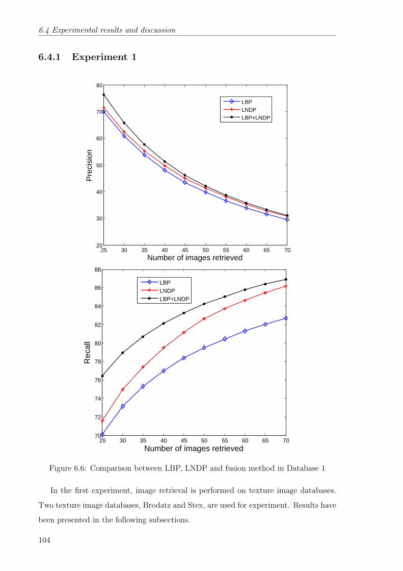
6.4 Experimental results and discussion
6.4.1 Experiment 1
25 30 35 40 45 50 55 60 65 7020
30
40
50
60
70
80
Number of images retrieved
Pre
cisi
on
25 30 35 40 45 50 55 60 65 7070
72
74
76
78
80
82
84
86
88
Number of images retrieved
Rec
all
LBPLNDPLBP+LNDP
LBPLNDPLBP+LNDP
25 30 35 40 45 50 55 60 65 7020
30
40
50
60
70
80
Number of images retrieved
Pre
cisi
on
25 30 35 40 45 50 55 60 65 7070
72
74
76
78
80
82
84
86
88
Number of images retrieved
Rec
all
LBPLNDPLBP+LNDP
LBPLNDPLBP+LNDP
Figure 6.6: Comparison between LBP, LNDP and fusion method in Database 1
In the first experiment, image retrieval is performed on texture image databases.
Two texture image databases, Brodatz and Stex, are used for experiment. Results have
been presented in the following subsections.
104

Chapter 6. Local Neighborhood Difference Pattern : A New Feature Descriptor
Database 1
Details about Brodatz database have been given in Chapter 1 Section 1.2.1. Precision
and recall have been calculated for the Brodatz database images using Eq. (1.6-1.11).
Images are retrieved in a group of 25, 30, 35,.., 70 to measure the performance of
system for different numbers in images. Graph between precision and number of images
retrieved is demonstrated in Fig. 6.5(a), and graph of recall and number of images
retrieved is shown in 6.5(b). Graphs clearly demonstrate that, as compared to other
methods, the proposed method is better in terms of both precision and recall. Average
retrieval rate (ARR) of all methods have been presented in table 1. ARR of the
proposed method is upgraded from CSLBP, LEPINV, LEPSEG, LBP, DLEP and LTrP
up to 35.46%, 34.45%, 17.98%, 9.06%, 7.03% and 3.09%. A query example has been
presented in Fig. 6.7, where (a) and (b) are query images, and similar images retrieved
using proposed method are shown. Comparisons of LBP and LNDP are individually
shown in Fig. 6.6. Performance of LNDP is better than LBP and the fusion of both
the methods has given much better results.
Retrieved ImagesQuery Image
(a)
(b)
Figure 6.7: Query image example of Brodatz database images
105
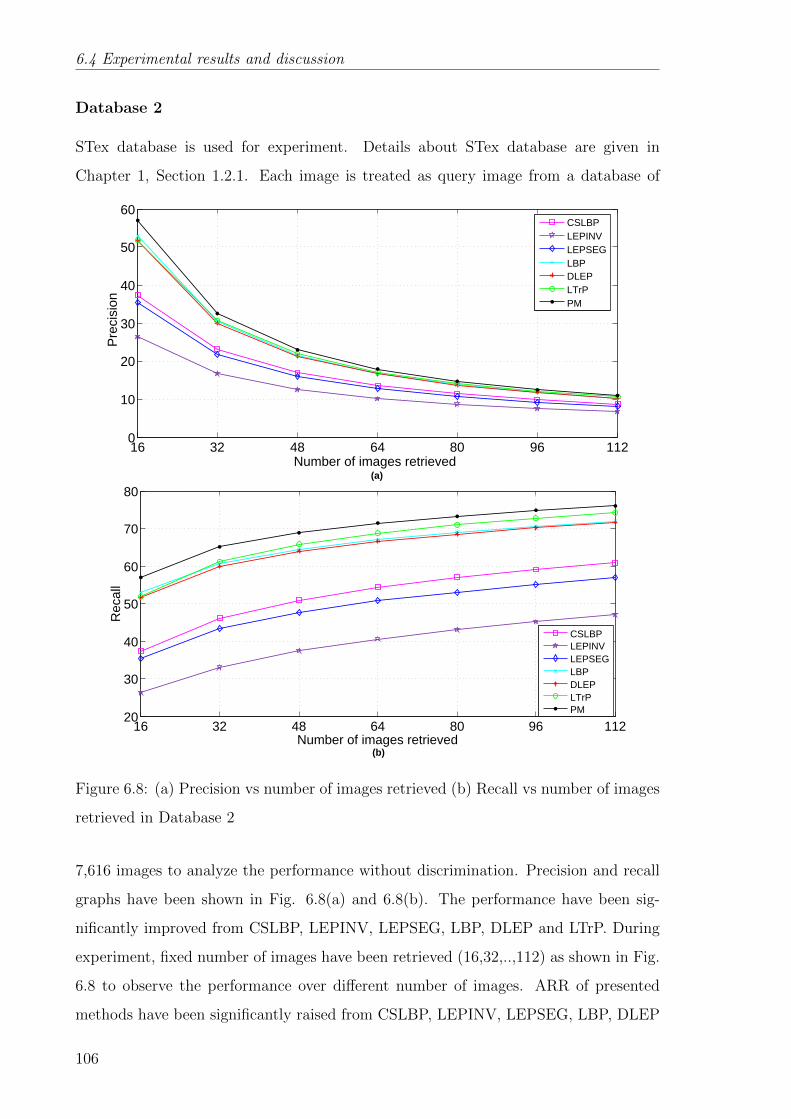
6.4 Experimental results and discussion
Database 2
STex database is used for experiment. Details about STex database are given in
Chapter 1, Section 1.2.1. Each image is treated as query image from a database of
16 32 48 64 80 96 1120
10
20
30
40
50
60
Number of images retrieved
Pre
cisi
on
CSLBPLEPINVLEPSEGLBPDLEPLTrPPM
(a)
16 32 48 64 80 96 11220
30
40
50
60
70
80
Number of images retrieved
Rec
all
CSLBPLEPINVLEPSEGLBPDLEPLTrPPM
(b)
Figure 6.8: (a) Precision vs number of images retrieved (b) Recall vs number of images
retrieved in Database 2
7,616 images to analyze the performance without discrimination. Precision and recall
graphs have been shown in Fig. 6.8(a) and 6.8(b). The performance have been sig-
nificantly improved from CSLBP, LEPINV, LEPSEG, LBP, DLEP and LTrP. During
experiment, fixed number of images have been retrieved (16,32,..,112) as shown in Fig.
6.8 to observe the performance over different number of images. ARR of presented
methods have been significantly raised from CSLBP, LEPINV, LEPSEG, LBP, DLEP
106

Chapter 6. Local Neighborhood Difference Pattern : A New Feature Descriptor
and LTrP up to 52.95%, 116.33%, 61.08%, 7.85%, 10.56% and 10.06%. Precision and
recall of LBP and LNDP separately demonstrated in Fig. 6.9. LNDP outperforms
LBP and fusion of both the methods has further improved the accuracy.
16 32 48 64 80 96 11210
20
30
40
50
60
Number of images retrieved
Pre
cisi
on
16 32 48 64 80 96 11250
55
60
65
70
75
80
Number of images retrieved
Rec
all
LBPLNDPLBP+LNDP
LBPLNDPLBP+LNDP
16 32 48 64 80 96 11210
20
30
40
50
60
Number of images retrieved
Pre
cisi
on
16 32 48 64 80 96 11250
55
60
65
70
75
80
Number of images retrieved
Rec
all
LBPLNDPLBP+LNDP
LBPLNDPLBP+LNDP
Figure 6.9: Comparison between LBP, LNDP and fusion method in Database 2
107
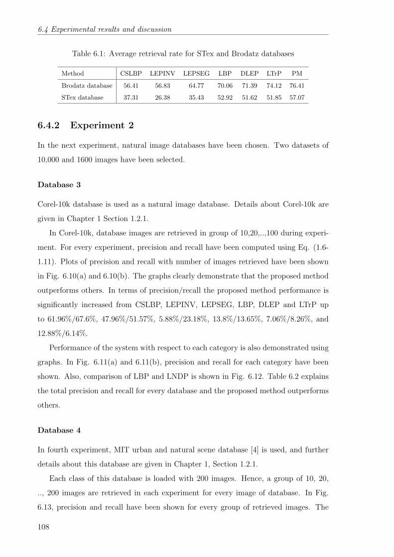
6.4 Experimental results and discussion
Table 6.1: Average retrieval rate for STex and Brodatz databases
Method CSLBP LEPINV LEPSEG LBP DLEP LTrP PM
Brodatz database 56.41 56.83 64.77 70.06 71.39 74.12 76.41
STex database 37.31 26.38 35.43 52.92 51.62 51.85 57.07
6.4.2 Experiment 2
In the next experiment, natural image databases have been chosen. Two datasets of
10,000 and 1600 images have been selected.
Database 3
Corel-10k database is used as a natural image database. Details about Corel-10k are
given in Chapter 1 Section 1.2.1.
In Corel-10k, database images are retrieved in group of 10,20,..,100 during experi-
ment. For every experiment, precision and recall have been computed using Eq. (1.6-
1.11). Plots of precision and recall with number of images retrieved have been shown
in Fig. 6.10(a) and 6.10(b). The graphs clearly demonstrate that the proposed method
outperforms others. In terms of precision/recall the proposed method performance is
significantly increased from CSLBP, LEPINV, LEPSEG, LBP, DLEP and LTrP up
to 61.96%/67.6%, 47.96%/51.57%, 5.88%/23.18%, 13.8%/13.65%, 7.06%/8.26%, and
12.88%/6.14%.
Performance of the system with respect to each category is also demonstrated using
graphs. In Fig. 6.11(a) and 6.11(b), precision and recall for each category have been
shown. Also, comparison of LBP and LNDP is shown in Fig. 6.12. Table 6.2 explains
the total precision and recall for every database and the proposed method outperforms
others.
Database 4
In fourth experiment, MIT urban and natural scene database [4] is used, and further
details about this database are given in Chapter 1, Section 1.2.1.
Each class of this database is loaded with 200 images. Hence, a group of 10, 20,
.., 200 images are retrieved in each experiment for every image of database. In Fig.
6.13, precision and recall have been shown for every group of retrieved images. The
108

Chapter 6. Local Neighborhood Difference Pattern : A New Feature Descriptor
25 30 35 40 45 50 55 60 65 7010
15
20
25
30
35
40
45
Number of images retrieved
Pre
cisi
on
25 30 35 40 45 50 55 60 65 702
4
6
8
10
12
14
16
18
Number of images retrieved
Rec
all
CSLBPLEPINVLEPSEGLBPDLEPLTrPPM
CSLBPLEPINVLEPSEGLBPDLEPLTrPPM
(a) (b)
25 30 35 40 45 50 55 60 65 7010
15
20
25
30
35
40
45
Number of images retrieved
Pre
cisi
on
25 30 35 40 45 50 55 60 65 702
4
6
8
10
12
14
16
18
Number of images retrieved
Rec
all
CSLBPLEPINVLEPSEGLBPDLEPLTrPPM
CSLBPLEPINVLEPSEGLBPDLEPLTrPPM
(a) (b)
Figure 6.10: (a) Precision vs number of images retrieved (b) Recall vs number of images
retrieved in Database 3
performance in terms of precision and recall is better than other methods as visible
in graphs. In terms of precision/recall, the performance of the proposed method is
109

6.4 Experimental results and discussion
0 5 10 15 20 25 30 35 40 45 50 55 60 65 70 75 80 85 90 95 10010
20
30
40
50
60
70
80
90
100
Image category
Pre
cisi
on
CSLBPLEPINVLEPSEGLBPDLEPLTrPPM
(a)
0 5 10 15 20 25 30 35 40 45 50 55 60 65 70 75 80 85 90 95 1000
10
20
30
40
50
60
70
80
Image category
Rec
all
CSLBPLEPINVLEPSEGLBPDLEPLTrPPM
(b)
Figure 6.11: (a) Precision vs image category (b) Recall vs image category in Database
3
significantly increased from CSLBP, LEPINV, LEPSEG, LBP, DLEP and LTrP up
to 25.84%/24.26%, 21.01%/18.73%, 13.19%/9.98%, 3.06%/13.08%, 5.29%/13.94% and
3.09%/0.45%.
Table 6.2: Results of precision and recall for all methods
MethodCorel-10k database MIT natural scene
Precision (n=10) Recall (n=100) Precision (n=10) Recall (n=200)
CSLBP 26.43 10.15 55.82 31.38
LEPINV 28.93 11.22 58.04 32.85
LEPSEG 34.01 13.81 62.06 35.46
LBP 37.62 14.97 68.16 34.49
DLEP 39.99 15.71 66.71 34.23
LTrP 37.93 16.03 68.14 38.82
PM 42.81 17.01 70.24 39.00
110
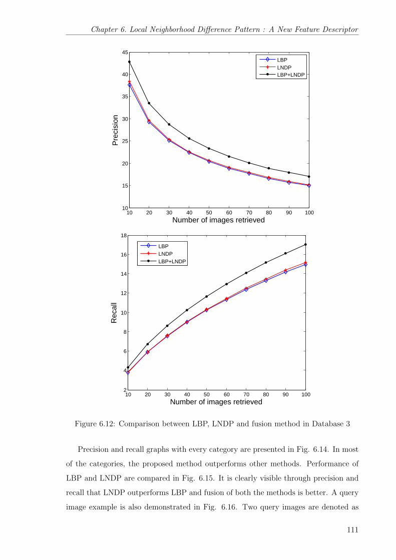
Chapter 6. Local Neighborhood Difference Pattern : A New Feature Descriptor
10 20 30 40 50 60 70 80 90 10010
15
20
25
30
35
40
45
Number of images retrieved
Pre
cisi
on
10 20 30 40 50 60 70 80 90 1002
4
6
8
10
12
14
16
18
Number of images retrieved
Rec
all
LBPLNDPLBP+LNDP
LBPLNDPLBP+LNDP
10 20 30 40 50 60 70 80 90 10010
15
20
25
30
35
40
45
Number of images retrieved
Pre
cisi
on
10 20 30 40 50 60 70 80 90 1002
4
6
8
10
12
14
16
18
Number of images retrieved
Rec
all
LBPLNDPLBP+LNDP
LBPLNDPLBP+LNDP
Figure 6.12: Comparison between LBP, LNDP and fusion method in Database 3
Precision and recall graphs with every category are presented in Fig. 6.14. In most
of the categories, the proposed method outperforms other methods. Performance of
LBP and LNDP are compared in Fig. 6.15. It is clearly visible through precision and
recall that LNDP outperforms LBP and fusion of both the methods is better. A query
image example is also demonstrated in Fig. 6.16. Two query images are denoted as
111

6.5 Conclusion
0 20 40 60 80 100 120 140 160 180 20030
40
50
60
70
80
Number of images retrieved
Pre
cisi
on
CSLBPLEPINVLEPSEGLBPDLEPLTrPPM
(a)
0 20 40 60 80 100 120 140 160 180 2000
5
10
15
20
25
30
35
40
Number of images retrieved
Rec
all
CSLBPLEPINVLEPSEGLBPDLEPLTrPPM
(b)
Figure 6.13: (a) Precision vs number of images retrieved (b) Recall vs number of images
retrieved in Database 4
(a) and (b), and the most similar eight images are retrieved and are shown as results.
Feature vector length of each method have been given in table 6.3.
6.5 Conclusion
In this chapter, a novel local feature descriptor has been proposed and called as local
neighborhood difference pattern (LNDP). The proposed local feature descriptor LNDP,
is a complementary method over LBP as it extracts the relationship among neighboring
pixels by comparing them mutually. On the contrary, LBP computes the relationship
of neighboring pixels with center pixel. In the proposed feature extraction method,
112

Chapter 6. Local Neighborhood Difference Pattern : A New Feature Descriptor
Coast & Beach Forest Highway City Center Mountain Open Country Street Tall Building
0.4
0.5
0.6
0.7
0.8
0.9
1
Image category
Pre
cisi
on
CSLBPLEPINVLEPSEGLBPDLEPLTrPPM
(c)
Coast & Beach Forest Highway City Center Mountain Open Country Street Tall Building0.1
0.2
0.3
0.4
0.5
0.6
Image category
Rec
all
CSLBPLEPINVLEPSEGLBPDLEPLTrPPM
(d)
Figure 6.14: (a) Precision vs image category (b) Recall vs image category in Database
4
Table 6.3: Feature vector length of different methods
Method Feature vector length
CS LBP 16
LEPINV 72
LEPSEG 512
LBP 256
DLEP 2048
LTrP 767
LNDP 256
LNDP+LBP 512
113

6.5 Conclusion
20 40 60 80 100 120 140 160 180 20030
35
40
45
50
55
60
65
70
75
Number of images retrieved
Pre
cisi
on
LBPLNDPLBP+LNDP
20 40 60 80 100 120 140 160 180 2000
5
10
15
20
25
30
35
40
Number of images retrieved
Rec
all
LBPLNDPLBP+LNDP
20 40 60 80 100 120 140 160 180 20030
35
40
45
50
55
60
65
70
75
Number of images retrieved
Pre
cisi
on
LBPLNDPLBP+LNDP
20 40 60 80 100 120 140 160 180 2000
5
10
15
20
25
30
35
40
Number of images retrieved
Rec
all
LBPLNDPLBP+LNDP
Figure 6.15: Comparison between LBP, LNDP and fusion method in Database 4
LBP and LNDP are combined as they complete each other on the basis of local feature
extraction. The proposed method has been applied in image retrieval of texture and
natural image datasets. Two texture datasets and two natural image datasets have
been chosen for experiments. The performance of proposed method has been observed
114

Chapter 6. Local Neighborhood Difference Pattern : A New Feature Descriptor
(b)
(a)
Query Image Retrived Images
Figure 6.16: Query image example of urban and natural scene database, MIT
using precision and recall graphs, and compared with some existing local patterns.
Evaluation measures clearly demonstrate that the proposed method outperforms other
methods in terms of accuracy.
115


Chapter 7
Object Tracking using Joint Histogram
of Color and Local Rhombus Pattern
Object tracking is a crucial issue in the field of pattern recognition and computer
vision. It mainly finds applications in the areas of vehicle navigation, traffic monitoring,
face tracking, etc. Object tracking has two major tasks, first is feature extraction of
the target object in the video sequence, and second is to track the target object in the
video sequence, using features.
In this chapter, a feature extraction method named local rhombus pattern (LRP)
is proposed, and it is different from the conventional local binary pattern as it extracts
the local relationship of neighboring pixels itself instead of local relationship with
the center pixel. The proposed method is combined with HSV (hue, saturation and
value) quantized histogram, and is applied to object tracking using mean shift tracking
algorithm. Experiments are carried out for road traffic and sports video, using joint
histogram of LRP and HSV color space, and compared to two state-of-art approaches.
The experimental results show the effectiveness of the proposed method over existing
methods.
117

7.1 Local rhombus pattern
7.1 Local rhombus pattern
Local rhombus pattern - 0111Local rhombus pattern value - 14
13 17 1118 16 1815 12 19
00 111 1
(a) (b)-51-33 1 7
(d) (e) (f)10 0
-701
(c)1
1 01
84 1
2
84 14 0
2(h) (i)(g)
I6 I7 I8
I5 Ic I1
I4 I3 I2
00 1
-4 1 -6
Figure 7.1: Local rhombus pattern sample window example
In the proposed method, features are derived using neighboring pixels that evaluate
the mutual relationship among neighboring pixels instead of the center pixel. Four
neighborhood pixels, two each in the vertical and horizontal directions have been used
for pattern formation. For each of the four pixels, two neighboring pixels are considered,
and relationships based on their comparison are extracted.
As shown in Fig. 7.1(a), I1, I3, I5 and I7 are considered for pattern formation.
A sample window of the image is given in Fig. 7.1(b), and steps involved in pattern
creation process are demonstrated in Fig. 7.1(c-f). Fig. 7.1(g-i) shows how the pattern
values are obtained from local rhombus pattern. In Fig. 7.1(c), the pixel I1 is sub-
tracted from pixel I2 and I8, and based on both difference values, a pattern is assigned
to I1. If both difference values are of different signs, i.e., positive and negative, then
‘0’ is assigned, and if both difference values are of same sign, i.e., both positive or both
118

Chapter 7. Object Tracking using Joint Histogram of Color and Local RhombusPattern
negative then ‘1’ is assigned to that pixel. Hence, in this example, 0, 1, 1 and 1 values
are assigned to I1, I3, I5 and I7, respectively. These values are further multiplied with
weights as mentioned in Fig. 7.1(h) and summed up to a single pattern value as shown
in Fig. 7.1(i). The four pixels which form a rhombus around the center pixel, are used
for pattern creation. Hence, this method is named as the local rhombus pattern.
For a pixel (x, y), LRP is formulated as follows:
T n1 = In−1 − In, T n2 = In+1 − In, ∀ n = 3, 5, 7. (7.1)
T n1 = I8 − In, T n2 = In+1 − In, for n = 1 (7.2)
F1(Tn1 , T
n2 ) =
1 T n1 × T n2 ≥ 0
0 else(7.3)
LRP (x, y) =3∑i=0
2i × F1(T2i+11 , T 2i+1
2 ) (7.4)
where In;n = 1, 2, ..., 8 are neighboring pixel positions as shown in Fig. 7.1(a), and
LRP (x, y) is local rhombus pattern value of pixel (x, y) in the image.
The proposed feature descriptor is motivated by the conventional local binary pat-
tern. LBP is a very strong feature descriptor but it has a high dimension for joint
histogram purpose. The modified rotation invariant uniform patterns [106] have less
feature vector length, however it loses information with feature reduction. The pro-
posed method, named local rhombus pattern (LRP) is based on mutual relationship
among neighboring pixels rather than the center pixel and neighboring pixel relation-
ship, and originally it has less feature vector length, and no further reduction is re-
quired. Hence, it is not losing extra information in reduction of feature vector length.
7.2 Framework of proposed algorithm
7.2.1 Target object representation
The proposed method is inspired by the local binary pattern that extracts the local
information based on neighboring pixels and center pixel [105]. Ning et al. used joint
histogram of LBP and RGB color channels for object tracking [102].
In the proposed work, the HSV color space is used for color information of the
target object. It separates the color component (hue), brightness (saturation) and
119

7.3 Experimental results and discussion
intensity (value) such that individual information regarding hue, saturation and value
can be extracted. Hue, saturation and value components of the HSV color space are
quantized in order to reduce the complexity of the algorithm. Hue, saturation and value
components are quantized into 18, 3 and 3 bins respectively. Texture information of
the object is created by LRP and joint histogram of LRP, and hue, saturation and
value components are generated. The local rhombus pattern has a total of 16 features,
and hue, saturation and value have 18, 3 and 3 bins respectively [171]. Hence, the total
length of histogram is 16×18×3×3. The target object is tracked in next frames using
mean shift tracking algorithm [22]. The algorithm for the proposed system is given in
the following sequence:
7.2.2 Algorithm
Input: Video sequence with location of the target object in the first frame.
Output: Tracked object in full video.
1. Upload the video and select the target object in the first frame for tracking.
2. Compute LRP of the target object in the first and next frame.
3. Convert the current and next frame from RGB to HSV color space, and quantize
hue, saturation and value bins to 18, 3 and 3 respectively.
4. Create joint histogram of hue, saturation, value and LRP for the target object
in the current and next frame.
5. Track the target object in the next frame using mean shift tracking algorithm
with joint HSV and LRP histogram.
6. Repeat the process from step 2 to 5 till the end frame.
7.3 Experimental results and discussion
In this work, two experiments on different videos have been conducted and the pro-
posed algorithm is compared with the following two algorithms.
120

Chapter 7. Object Tracking using Joint Histogram of Color and Local RhombusPattern
LBPriu2 RGB : Rotation invariant uniform local binary pattern + RGB color his-
togram [102]
LEP RGB : Local extrema pattern + RGB color histogram [93].
The proposed method is abbreviated as LRP HSV. In each experiment, the target
object is selected manually and marked as a red box. Our algorithm first extracts
features, and then tracks the required object in the next frames.
In the first experiment, a video of nearly similar moving cars is used. The video
Frame 1
Frame 90 Frame 120
(a)Frame 160 Frame 201
Frame 45Frame 20 Frame 64Frame 63
Frame 140
Frame 1 Frame 20 Frame 45 Frame 63 Frame 64
Frame 90 Frame 120 Frame 160 Frame 201Frame 140(b)
Frame 63Frame 20 Frame 45 Frame 64Frame 1
Frame 201Frame 160(c)
Frame 140Frame 120Frame 90
Figure 7.2: Object tracking in road traffic video using (a)LBPriu2 RGB (b) LEP RGB
and, (c) LRP HSV
121
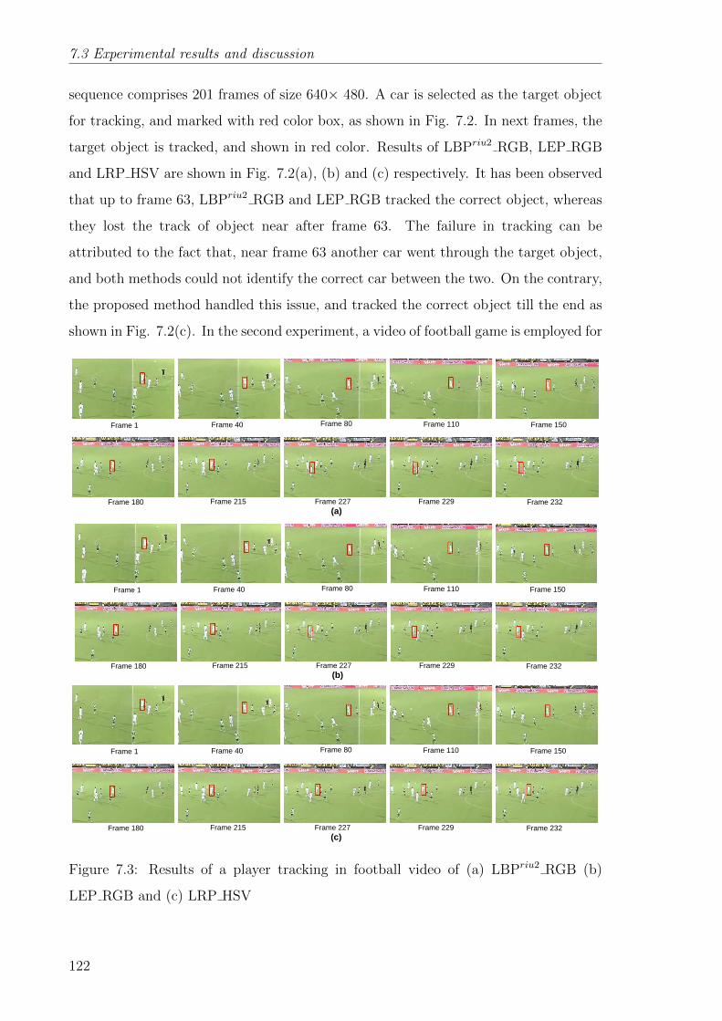
7.3 Experimental results and discussion
sequence comprises 201 frames of size 640× 480. A car is selected as the target object
for tracking, and marked with red color box, as shown in Fig. 7.2. In next frames, the
target object is tracked, and shown in red color. Results of LBPriu2 RGB, LEP RGB
and LRP HSV are shown in Fig. 7.2(a), (b) and (c) respectively. It has been observed
that up to frame 63, LBPriu2 RGB and LEP RGB tracked the correct object, whereas
they lost the track of object near after frame 63. The failure in tracking can be
attributed to the fact that, near frame 63 another car went through the target object,
and both methods could not identify the correct car between the two. On the contrary,
the proposed method handled this issue, and tracked the correct object till the end as
shown in Fig. 7.2(c). In the second experiment, a video of football game is employed for
Frame 1 Frame 40 Frame 80 Frame 110 Frame 150
Frame 180 Frame 215 Frame 227 Frame 229 Frame 232(a)
Frame 1 Frame 40 Frame 80 Frame 110 Frame 150
Frame 180 Frame 215 Frame 227 Frame 229 Frame 232(b)
Frame 1 Frame 40 Frame 80 Frame 110 Frame 150
Frame 180 Frame 215 Frame 227 Frame 229 Frame 232(c)
Figure 7.3: Results of a player tracking in football video of (a) LBPriu2 RGB (b)
LEP RGB and (c) LRP HSV
122

Chapter 7. Object Tracking using Joint Histogram of Color and Local RhombusPattern
the purpose of tracking one player. The tracking results of all three methods have been
demonstrated in Fig. 7.3. At the beginning of the video, all three algorithms worked
equally well and tracked the correct object. This is because the target object was almost
in isolation, and no disturbing objects were presented nearby. Whereas, towards end
frames, LBPriu2 RGB and LEP RGB missed the target object, and started tracking
other spurious objects. The reason for incorrect tracking is that towards the end video
frames, other players with similar appearance have come close to the target object, and
both methods have failed to distinguish the target object from other objects. Whereas,
in the proposed method, the target object is tracked correctly till the end of the video,
and are shown in Fig. 7.3(c).
Feature vector length and tracking time of all three methods are given in the table
7.1. Computation time depends on complexity of feature extraction method as well as
feature vector length. Feature vector length of LRP HSV is considerably less than of
LBPriu2 RGB and LEP RGB, hence, computation time is also less than LBPriu2 RGB
and LEP RGB.
Table 7.1: Feature vector length and process time of proposed method and previous
methods
Method Feature vector length Time taken
LBPriu2 RGB 10× 8× 8× 8 = 5120 1:08
LEP RGB 16× 8× 8× 8 = 8192 1:15
LRP HSV 16× 18× 3× 3 = 2592 1:02
7.4 Conclusion
A novel algorithm in the field of object tracking is proposed for feature extraction.
The proposed LRP extracts the local relationship among neighboring pixels for texture
features, and the HSV color space is used for color features. Next, a joint histogram
is constructed for color-texture features. The proposed method is applied to object
tracking application. Object tracking is performed on two video sequences of traffic
and sports using mean shift tracking algorithm. Experiments have been conducted
on a car traffic video and a football sport video. Experimental results prove that the
123

7.4 Conclusion
proposed algorithm has an important advantage over other methods that it is able to
track correct objects in similar looking objects in the video. It can be very useful in
traffic monitoring and other tracking applications.
124

Chapter 8
A Hierarchical Shot Boundary De-
tection Algorithm
A video is considered as high dimensional data which is tedious to process. Shot
detection and key frame selection are activities to reduce redundant data from a video
and make it presentable in few images. Researchers have worked in this area diligently.
Usually in video clips, shots repeat after one another, in that case the basic shot
detection scheme gives redundant key frames from same video. In a conversation video
or in general, shots usually repeat after one or more shots.
Basic shot detection schemes provide shot boundaries in a video sequence and key
frames are selected based on each shot. Usually in video clips, shots repeat after one
another, in that case the basic shot detection scheme gives redundant key frames from
same video. In this work, we have proposed a hierarchical shot detection and key
frames selection scheme which reduce a considerable amount of redundant key frames.
For temporal analysis and abrupt transformation detection, color histogram has been
used. After shot detection, spatial analysis has been done using local features and local
binary patterns have been utilized for local feature extraction. The proposed scheme is
applied to three video sequences of news video, movie clip and tv-advertisement video.
125

8.1 Hierarchical clustering for shot detection and key frame selection
In a video, many shots may be similar in visualization. In a conversation video or in
general, shots usually repeat after one or more shots. Usually, shot boundary detection
algorithms classify all shots in different clusters irrespective of redundant shots. In the
proposed method, the authors have developed a hierarchical shot detection algorithm
in two stages. First stage extracts temporal information of video and detect the initial
shot boundary and extract the keyframes based on each shot. In the second stage,
spatial information of extracted key frames from first stage are analyzed, and redundant
keyframes are excluded.
Figure 8.1: Consecutive frames and shot boundary of a video
8.1 Hierarchical clustering for shot detection and
key frame selection
Shot detection problem is very common in video processing. Processing a full video
at a time and extracting shot boundary may give results of similar shots. Frames of a
video are shown in Fig. 8.1. Ten different shots are there in the video, in which 3, 5
and 7, and 4, 6 and 8 are of similar kind. Hence, keyframes extracted from these shots
would be similar, and redundant information will be extracted from the video. It is a
small example and it can happen in large video. To solve this problem, a hierarchical
scheme has been adopted for keyframe extraction from a video.
For abrupt shot boundary detection, we have used RGB color histogram. RGB
color histogram provides global distribution of three color bands in RGB space. A
quantized histogram of 8 bins for each color channel has been created. Initially, each
color channel has been quantized in 8 intensities and histogram has been generated
126

Chapter 8. A Hierarchical Shot Boundary Detection Algorithm
using the following equation.
HistC(L) =m∑a=1
n∑b=1
F (I(a, b, C), L)
where C = 1, 2, 3 forR,G,B color bands
(8.1)
F (a, b) =
1 if, a = b
0 else.(8.2)
where size of the image is m× n and L is total number of bins that is ranging from 0
to 7. I(a, b, C) is the intensity of color channel C at position of (a, b).
For temporal information in a video sequence, each frame of video has been ex-
tracted and RGB color histogram has been generated. Difference of each frame to the
next frame is extracted using the following distance measure.
Dis(I1, I2) =l∑
s=1
|FI1(s)− FI2(s)| (8.3)
where Dis(I1, I2) is the distance between frame I1 and I2. FI1 and FI2 are feature
vectors of frame I1 and I2, and l is the feature vector length. If the measured distance
between two frames is greater than a fixed threshold value, then those frames are
separated in different clusters. This process is applied for each consecutive pair of
frames in video sequence. In this process, we get different clusters of similar frames.
After getting clusters, we extract one key frame from each cluster. For keyframe
extraction, entropy is calculated for every frame in one cluster using Eq. 8.4, and the
maximum entropy frame has been chosen as a keyframe for that cluster.
Ent(I) = −∑i
(pi × log2(pi)) (8.4)
where p is the histogram for the intensity image I.
During this process, consecutive keyframes will not hold the similar information.
However, except consecutive positions, two or more non-consecutive clusters may con-
tain similar types of frames as a video sequence may hold similar shots at non-consecutive
positions. Due to this, many keyframes may hold redundant information. To overcome
this issue, hierarchical process is adopted in this work. Local binary pattern (LBP) is
a well-known texture feature descriptor [106]. It computes relation of each pixel with
neighboring pixels. Explanation about LBP is given in detail in Chapter 5, Section
127

8.2 Proposed system framework
5.1.1. LBP is extracted from each of the keyframe obtained from the above process.
Now, the distance between each frame is mutually calculated using Eq. 8.3 as shown
in Fig. 8.2. Distance of frame 1 has been calculated with frame 2, 3 up to n. Distance
of frame 2 has been calculated with frame 3, 4 up to n. In a similar process, distance of
frame n− 1 has been calculated with frame n. A tri-diagonal matrix has been created
for all the distance measures. Now, if the distance between two or more frames is
less than a fixed threshold, then all those frames are grouped into one cluster. In this
process, even non-consecutive similar keyframes have been clustered, and completely
non-redundant data in different clusters have been obtained. Again, the entropy of
each of the frames in different cluster is calculated, and maximum entropy frame is ob-
tained as final keyframe. Finally, we get a reduced number of final key frames without
any redundant information.
1 2 3 n-1
2 3 4 n
Figure 8.2: Distance measure calculation in 2nd phase
8.2 Proposed system framework
8.2.1 Algorithm
Phase 1:
Input : Video clip
Output: Initial key frames
Upload video and extract all frames.
for i=1: n1
Calculate the RGB histogram of frame i and i+1.
Calculate Dist(i,i+1).
128

Chapter 8. A Hierarchical Shot Boundary Detection Algorithm
If(Dist(i,i+1)> Th1)
put i and i+1 in different clusters.
end
end
Calculate the entropy of each frame in different clusters.
Select maximum entropy frame from each cluster as a keyframe.
n1=total number of frames in video
Phase 2: Input : Initial key frames
Output: Selected final key frames
Load all keyframes extracted from Phase 1 and calculate LBP histogram for all.
Compute distance as explained in Fig. 8.2 and make a distance matrix ‘D’ for all
frames.
Initialize a zero vector key array of size n2.
for i=1: n2
If(key array(i))=0)
assign key array(i)=1
Initialize a Stack ‘S’ of size n2 and push first element i.
while(S is not empty)
t1= pop an element from S
Check if the distances between t1 and other frames are less than Th2 then
put them in one cluster t2.
Push all the elements of t2 in the Stack ‘S’.
end
Delete redundant frames from cluster if there is any.
else
continue
end
end
Calculate the entropy of each frame in different clusters.
Select maximum entropy frame from each cluster as a keyframe.
n2= number of keyframes extracted from Phase 1.
129

8.3 Experimental results
8.3 Experimental results
For experimental purpose, we have used three different videos of news, advertisement
and movie clip. General details about all three videos are given in table 8.1. All three
videos are of different size with respect to time and frame size. In news video, anchor
Table 8.1: Video details
Video Time(min.) Frame size Frame/sec
News video 02:55 1280× 720 30
Movie clip 00:30 720× 384 29
Advertisement 01:00 1920× 1080 25
and guest are present at first. The camera is moving from anchor to guest and guest
to anchor many times in the video. Hence, in shot detection, many shots are having
similar kind of frames (either anchor or guest). Further, other events are shown in
the video repeatedly one after another shot. All these redundant shots are separated
initially and key frames are selected. In the second phase of algorithm, redundant key
frames are clustered and keyframes of maximum entropy are extracted as final key
frames. Initially, 63 key frames are extracted and after applying hierarchical process
only 12 key frames are extracted at the end. This hierarchical process has removed a
significant amount of redundant key frames for further processing.
Second video for the experiment is a small clip of a animation movie called ‘Ice
age’. In this video, conversation between animated character of lion, elephant and
other animals are shown. Camera is moving from one kind of frames to other kind
of frames. The same hierarchical process is applied to the video clip. Initially, 11
key frames are extracted as shown in Fig. 8.3(a). However, many frames are similar
that is clearly visible in results, and then by using LBP for spatial information, 6 final
non-redundant key frames are extracted. In Fig. 8.3(b) keyframes of final phase have
been demonstrated.
The third video is taken for experiment is of a Tata-sky advertisement. The pro-
posed method is applied to the video and two phase keyframes are collected. The
keyframes of phase one and two are shown in Fig. 8.4. It is clearly visible that us-
ing hierarchical method, the number of key frames has been reduced significantly and
130

Chapter 8. A Hierarchical Shot Boundary Detection Algorithm
Figure 8.3: Video 1: (a) Initial stage keyframes (b) final stage keyframes
redundant key frames have been removed. Information regarding extracted key frames
in phase one and two are given in table 8.2. Summary of reduced keyframes explains
that the proposed algorithm has removed the repeated frames from key frames detected
from the color histogram method. Further, in phase two using LBP, we have obtained
optimum amount of key frames which summarize the video significantly.
Table 8.2: Number of keyframes extracted in both phases
Video Keyframes in Phase 1 Keyframes in Phase 2
News video 63 12
Movie clip 11 6
Advertisement 34 11
131

8.4 Conclusions
Figure 8.4: Video 1: (a) Initial stage keyframes (b) Final stage keyframes
8.4 Conclusions
In the proposed work, shot boundary detection problem has been discussed and further,
key frames have been obtained. A hierarchical approach is adopted for final keyframes
selection. This approach helped in reducing similar keyframes in non-consecutive shots.
Initially, a color histogram technique is used for temporal analysis and abrupt transition
is obtained. Based on abrupt transition, shots are separated and keyframes are selected.
Moreover, spatial analysis has been done in obtained keyframes using local binary
pattern and finally redundant keyframes are removed. In this process, a significant
amount of redundant keyframes are removed. The proposed method is applied on
three videos of news reading, movie clip and tv advertisement, and experiments show
that the proposed algorithm helped in removing redundant keyframes.
132

Chapter 9
Conclusions and Future Scope
9.1 Conclusions
In this work, we have presented texture features for different pattern recognition appli-
cations which includes content based image retrieval, object tracking and shot bound-
ary detection. Also, combination of image features (color and texture) is measured
to enhance the feature description. Proposed methods are demonstrated on publicly
available databases.
In content based image retrieval, feature extraction is a dominant step that can lead
the whole retrieval system in a positive or negative direction. Image feature extraction
in image retrieval application extremely depends on image database which have been
used to match the query image. Texture is a noticeable feature of image that can be
found in most of the kind images. Texture might be represented as a repeated pattern
in the image and can be extracted in a good way using local features.
An attempt has been made to extract local features using wavelet domain in Chap-
ter 2. Wavelet domain gives subband image which contains directional information.
Further, local patterns were used to extract local features of those subband images.
Local extrema patterns (LEP) [93] and directional local extrema patterns (DLEP) [95]
133

9.1 Conclusions
were proposed by Murala et al. Both of them are local feature descriptors that extracts
local information base on four directions. Discrete wavelet transform (DWT) captures
the low frequency and high frequency features and helps LEP and DLEP to create
more detailed features. Experiments are done on Corel-5k and Corel-10k databases
and both the methods have compared with some existing local patterns. Both the
methods are better in performance from other method. Although, performance of
proposed method 2 (DWT+DLEP) is better than proposed methods 1 (DWT+LEP).
On the other hand, feature vector length of proposed method 1 is less than proposed
method 2, hence proposed method 1 is faster than proposed method 2 in computation.
Image retrieval problem is solved using color and texture features in Chapter 2. HSV
color space is used for color descriptor and combined with texture descriptor. Hue and
saturation components are used for color information and value component is used to
extract texture features with the help of GLCM and LEP. GLCM extract the pixel pair
relation in terms of occurrence in image. Initially, LEP is extracted from value compo-
nent for local pattern information. Further, for each pixel pair, information is collected
using GLCM. The proposed method is using co-occurrence information of local extrema
pattern, hence it is called local extrema co-occurrence pattern (LECoP). To combine
color and texture features a joint histogram is created for hue saturation and LECoP.
The proposed method’s effectiveness is tested on three natural (Corel-1k, Corel-5k and
Corel-10k) and two color-texture (MIT VisTex and STex) image databases. The pro-
posed technique is compared with some color-texture features and proved its excellence
in terms of precision, recall and F-measure curves. The performance (precision %, recall
%) of the proposed (52.50,23.29) method has been improved from CS LBP+colorhist
(44.08, 18.57), LEPSEG+colorhist (35.58, 13.48), LEPINV+colorhist (41.25, 15.74) ,
Wavelet+colorhist (42.28, 17.34), Joint LEP colorhist (44.14, 16.77), Joint colorhist
(43.96,16.66) in Corel-10k database. Similarly in STex texture database (ARR %)
of the proposed (74.15) method has been improved from CS LBP+colorhist (53.33),
LEPSEG+colorhist (46.37), LEPINV+colorhist (48.10) , Wavelet+colorhist (45.08),
Joint LEP colorhist (59.90), Joint colorhist (59.90) in Corel-10k database. Further,
performance of the proposed method is evaluated using four distance measure in which
d1 distance has been proved the best among four. The main contribution of this work
is to extract pixel pair information in local patterns and it is noticed that it worked
134

Chapter 9. Conclusions and Future Scope
effectively. Chapter 3 is also based on a co-occurrence pattern using pixel pair infor-
mation. In Chapter 3, center symmetric local binary pattern (CSLBP) is extracted
from the original gray scale image. Co-occurrence matrix is collected from CSLBP
map in different directions and distances. Performance of the system is measured on
different combinations of directions and distances and four combinations are chosen
to collect the features. Combinations of 1 and 2 distances and 0◦, 45◦, 90◦ and 135◦
directions are used to extract feature and integrated in one feature vector. With this,
we are getting co-occurrence information in different directions. This method can be
treated as a rich texture feature descriptor as it contains local pattern information with
co-occurrence in different distance and directions. This feature descriptor is tested on
textural (MIT VisTex, Brodatz), facial (ORL face database) and bio-medical (OASIS
MRI) image database and compared with existing local feature descriptors. The pro-
posed method has proved its significance in all different types of databases. Hence, it
can be performed in different pattern recognition applications as a texture feature.
In chapter 4, a novel feature descriptor called, local tri-directional pattern has been
proposed. This local pattern is an extened version of LBP and it extracts local infor-
mation based on the difference neighboring pixels in three direction. Using the same
three directions, one magnitude pattern is extracted and both patterns are combined
to extract features for CBIR system. The proposed feature descriptor are applied to
textural (MIT VisTex and Brodatz) and facial (ORL face database) image databases.
A new feature extraction method is proposed in chapter 5 and named as local neigh-
borhood difference pattern. The proposed feature descriptor transforms the mutual
relationship of all neighboring pixels in a binary pattern. Both LBP and LNDP are
opposite to each other as they obtain different information using local pixels. In the
proposed CBIR system, both LBP and LNDP features are combined. To prove the
excellence of the proposed method, four different database of textural images (STex
and Brodatz) and natural images (Corel-10k and MIT natural and urban scene image
database) are used. Performance has been analyzed using precision and recall for all
databases and compared with some existing local patterns. Performance of the pro-
posed method (70.24, 39.00) in terms of (precision %, recall %) has been improved
from CSLBP (55.82, 31.38), LEPINV (58.04, 32.85), LEPSEG (62.06, 35.46), LBP
135

9.2 Future scope
(68.16, 34.49), DLEP (66.71, 34.23), LTrP (68.14, 38.82) in MIT natural and urban
scene database.
In chapter 6, local rhombus pattern is proposed for texture features and combined
with HSV color histogram and applied to object tracking. Object tracking requires
many steps for processing. In this work, only feature extraction method is proposed
that is a very crucial step. To track the object, mean shift tracking algorithm is used.
The proposed method is tested on football sports and car traffic video sequences and
compared with existing LBP [102] and LEP [93] based tracking algorithms. Visual
results have been shown using frames and observed that the proposed method worked
fine when two similar objects are near or crossing each other whereas earlier approaches
failed to recognize actual object.
A shot detection problem is solved for reducing the repetitive keyframes in a video.
Shot detection is common problem in video analysis. After shot detection, keyframe ex-
traction need to be done that makes a video ready for further process as it reduces huge
amount of data. However, still there exist many similar keyframes which make a sys-
tem slow in further process. A hierarchical approach is proposed using color histogram
and local binary pattern. The proposed method is tested on three video sequences.
Initial keyframe detection is performed using color histogram. Final keyframes are
extracted from a set of initial keyframes using LBP. Experiment results shows that the
hierarchical approach has reduced a huge amount of data.
9.2 Future scope
The presented work in this thesis leaves some scope to extend the work in computer
vision applications. Some of them are as follows:
1. The proposed features can be utilized in secure image retrieval using encryption
techniques.
2. Proposed feature are mainly based on texture and few are integrated with color
features. Integration of shape features with proposed techniques might used to
enhance the image feature extraction.
136

Chapter 9. Conclusions and Future Scope
3. In chapter 6, feature are extracted using closest neighborhood in LNDP and LBP
in radius one. Extended neighborhood can be used for feature extraction. As
LBP has proved better features in extended neighborhood for radius two and
three, LNDP can be utilized in a similar way along with LBP.
4. Proposed feature descriptors are based on texture and rich in extracting in texture
information. They can be utilized for video retrieval and image based video
retrieval.
5. Proposed hierarchical shot detection approach can be utilized for a video retrieval
system.
137


Appendix
The proposed methods in this thesis are compared with some existing methods.
Few of them are already explained in thesis chapters since they are required as a prior
knowledge for proposed techniques. Local binary pattern (LBP), local ternary pattern
(LTP), local extrema pattern (LEP), directional local extrema pattern (DLEP) and
center symmetric local binary pattern (CSLBP) are explaned in detail in previous
chapters. For LBP, values of P and R are taken as 1 and 8 respectively (nearest
neighboring pixels). For CSLBP, values of P, R and T are taken as 1, 8 and 2.6
respectively. (Refer the previous chapters for explanation)
Rest of the techniques which are used in comparison are explained below:
Local tetra pattern (LTrP)
Murala et al. proposed local tetra pattern (LTrP) [96]. Given image I, the first-order
derivatives along 0◦ and 90◦ directions are denoted as I1θ |θ=0◦,90◦ . Let gc denote the
center pixel in I, and let gh and gv denote the horizontal and vertical neighborhoods
of gc, respectively. Then, the first-order derivatives at the center pixel can be written
as
I10◦(gc) = I(gh)− I(gc) (9.1)
I190◦(gc) = I(gv)− I(gc) (9.2)
139

Appendix
and the direction of the center pixel can be calculated as
I1Dir.(gc) =
1, I10◦(gc) ≥ 0 and I190◦(gc) ≥ 0
2, I10◦(gc) < 0 and I190◦(gc) ≥ 0
3, I10◦(gc) < 0 and I190◦(gc) < 0
4, I10◦(gc) ≥ 0 and I190◦(gc) < 0
(9.3)
From 9.2, it is evident that the possible direction for each center pixel can be either 1,
2, 3, or 4, and eventually, the image is converted into four values, i.e., directions.
The second-order LTrP 2(gc) is defined as
LTrP 2(gc) = {f1(I1Dir.(gc), I1Dir.(g1)), f1(I1Dir.(gc), I1Dir.(g2)), ..., f1(I1Dir.(gc), I1Dir.(gP ))}|P=8
(9.4)
f1(I1Dir.(gc), I
1Dir.(gP )) =
0, I1Dir.(gc) = I1Dir.(gP )
I1Dir.(gP ), else(9.5)
From 9.4 and 9.5, 8-bit tetra patterns have been obtained for each center pixel. Then,
they are separated into four parts based on the direction of center pixel. Finally, the
tetra patterns for each part (direction) are converted to three binary patterns.
Let the direction of center pixel (I1Dir.(gc)) obtained using 9.3 be“1; then, LTrP 2
can be defined by segregating it into three binary patterns as follows:
LTrP 2|Direction=2,3,4 =P∑p=1
2p−1 × f2(LTrP 2(gc))|Direction=2,3,4 (9.6)
f2(LTrP2(gc))|Direction=φ =
1, if LTrP 2(gc) = φ
0, else(9.7)
where φ = 2, 3, 4.
Similarly, the other three tetra patterns for remaining three directions (parts) of
center pixels are converted to binary patterns. Thus, there are 12 (4×3) binary pat-
terns. Magnitude pattern (LP) has been obtained using following equations:
MI1(gp) =√
(I10◦(gp))2 + (I190◦(gp))
2 (9.8)
LP =P∑p=1
2p−1 × f3(MI1(gp) −MI1(gc))|P=8 (9.9)
f3(x) =
1, if x ≥ 0
0, else(9.10)
140

Appendix
To reduce the feature vector length, uniform patterns have been used. The uniform
pattern refers to the uniform appearance pattern that has limited discontinuities in the
circular binary representation. In this method, those patterns that have less than or
equal to two discontinuities in the circular binary representation are referred to as the
uniform patterns, and the remaining patterns are referred to as nonuniform. Thus, the
distinct uniform patterns for a given query image would be P (P − 1) + 2.
Histogram of LTrP is calculated as follows:
HLTrP (l) =
N1∑j=1
N2∑k=1
f(LTrP (j, k), l), l ∈ [0, 58] (9.11)
f(x, y) =
1 x = y
0 else(9.12)
For each pattern histogram length is 59 (0 to 58 pattern values). In LTrP, total 13
histograms are there, hence total lenght of histogram would be 59× 13.
Local maximum edge binary pattern (LMEBP)
LMEBP was proposed by Murala et al. In this method, for a given image the first
maximum edge is obtained by the magnitude of local difference between the center
pixel and its eight neighbors as shown below:
I′(gi) = I(gi)− I(gc), i = 1, 2, ..., 8 (9.13)
i1 = argi
(max(|I ′(g2)|, ..., |I ′(g8)|)) (9.14)
where max(x) calculates the maximum value in an array x. If this edge is positive,
assign ‘1 to this particular center pixel otherwise‘0.
Inew(gc) = f4(I′(gi1)) (9.15)
f4(x) =
1 x ≥ 0
0 else(9.16)
The LMEBP is defined as
LMEBP (I(gc)) = {Inew(gc); Inew(g1); I
new(g2); ...Inew(g8)} (9.17)
141

Appendix
Eventually, the given image is converted to LMEBP image having values ranging from
0 to 511.
After calculation of LMEBP, the whole image is represented by building a histogram
supported by
HLMEBP (l) =
N1∑j=1
N2∑k=1
f(LMEBP (j, k), l), l ∈ [0, 511] (9.18)
where the size of input image is N1 ×N2. Similarly, the remaining seven LMEBPs
are evaluated using seven maximum edges (second maximum edge to eighth maximum
edge) to obtain eight LMEBP histograms. Hence the feature vector of this method is
8 × 512.
Local edge pattern (LEPSEG and LEPINV)
Local edge patterns (LEP) were proposed by Yao and Chen in 2003 [168]. To compute
the LEP value, an edge image must be obtained first. The edge image is obtained by
applying the Sobel edge detector to gray level image.
LEPSEG(n,m) =∑i,j∈I
ke(i, j)× e(n,m),
ke(i, j) =
1 2 4
128 256 8
64 32 16
(9.19)
where e(n,m) denotes the binary edge image (obtained using Sobel operator), I is a 3
3 neighborhood, ke(i, j) is the LEP mask, and LEPSEG(n,m) is the output LEPSEG
value at the pixel located at (n,m). Accordingly, the LEPSEG histogram he′(01) for a
texture region R is obtained using the following equation:
he′(01)i =
n′(01)i
N (0), i = 0, 1, 2, ..., 511. (9.20)
where n′(01)i is the number of pixels with LEPSEG value i and N is the number of
total pixels in R. The LEPSEG value LEPSEG(n,m) as speci1ed by Eq. 9.19 can
be expressed by a binary string b8b7b6b5b4b3b2b1b0. After the most signi1cant bit corre-
sponding to the central pixel is excluded, a number of binary shifts is then applied to
the 8-bit binary string b8b7b6b5b4b3b2b1b0 until the value represented by the bit string
142

Appendix
is the least value. After the processing, there are only 36 different least values derived
from the 8-bit binary string. Obviously, the 36 values are rotation invariant since only
the sequence of the bit string is concerned rather than its starting point. After the most
signi1cant bit corresponding to the central pixel is excluded from 0000011110, the bit
strings 000011110, 000111100 001111000 11110000, 111000001, 110000011, 100000111
and 000001111 have the same least value 15. However, the 36 values do not describe
whether or not the central pixel is an edge pixel. Thus, if the central pixel is an edge
pixel then 36 is added, leading to a LEPROT value.The LEPROT values are divided
into two parts depending on whether or not the central pixel of the neighborhood is
an edge pixel. In this way two LEPINV histograms,he(0) and he(1) can be obtained for
a texture region R using the following equation:
he(0)i =
niN (0)
(9.21)
he(1)i =
ni+36
N −N (0)(9.22)
where ni is the number of pixels with LEPROT value i and N (0) is the number of total
non-edge pixels in R.
143


Bibliography
[1] “Corel-1k database,” Availble online : http://wang.ist.psu.edu/docs/related/,
(last accessed on 11/12/2015).
[2] “Corel-5k and Corel-10k database,” Available online :
http://www.ci.gxnu.edu.cn/cbir/, (last accessed on 8/10/2014).
[3] “MIT vision and modeling group, Cambridge, vision texture,” Available online :
http://vismod.media.mit.edu/pub/, (last accessed on 11/12/2015).
[4] “Urban and natural scene categories, computational visual cognition
laboratory, Massachusetts Institute of Technology,” Available online :
http://cvcl.mit.edu/database.htm, (last accessed on 11/12/2015).
[5] “The AT&T database of faces, AT&T laboratories Cambridge,” Avaiable
online : http://www.cl.cam.ac.uk/research/dtg/attarchive/facedatabase.html,
2002, (last accessed on 11/12/2015).
[6] A. Ahmadian and A. Mostafa, “An efficient texture classification algorithm us-
ing gabor wavelet,” in Proceedings of 25th Annual International Conference of
Engineering in Medicine and Biology Society vol., 1. Cancun, Mexico: IEEE,
2003, pp. 930–933.
145

BIBLIOGRAPHY
[7] T. Ahonen, A. Hadid, and M. Pietikainen, “Face recognition with local bi-
nary patterns,” in Proceedings of 8th European Conference on Computer Vision.
Prague, Czech Republic: Springer, 2004, pp. 469–481.
[8] P. Anantharatnasamy, K. Sriskandaraja, V. Nandakumar, and S. Deegalla, “Fu-
sion of colour, shape and texture features for content based image retrieval,” in
Proceedings of 8th International Conference on Computer Science & Education
(ICCSE). Colombo, Sri Lanka: IEEE, 2013, pp. 422–427.
[9] E. Apostolidis and V. Mezaris, “Fast shot segmentation combining global and lo-
cal visual descriptors,” in Proceedings of the International Conference on Acous-
tics, Speech and Signal Processing (ICASSP). Florence, Italy: IEEE, 2014, pp.
6583–6587.
[10] J. Baber, S. Satoh, N. Afzulpurkar, and M. Bakhtyar, “Q-CSLBP: compression
of CSLBP descriptor,” in Advances in Multimedia Information Processing–PCM.
Singapore: Springer, 2012, pp. 513–521.
[11] R. V. Babu and P. Parate, “Robust tracking with interest points: A sparse
representation approach,” Image and Vision Computing vol., 33, pp. 44–56,
2015.
[12] A. Baraldi and F. Parmiggiani, “An investigation of the textural characteris-
tics associated with gray level cooccurrence matrix statistical parameters,” Geo-
science and Remote Sensing, IEEE Transactions on vol., 33, no. 2, pp. 293–304,
1995.
[13] A. C. Bovik, Handbook of image and video processing. Academic press, 2010.
[14] S. Brandt, J. Laaksonen, and E. Oja, “Statistical shape features for content-
based image retrieval,” Journal of Mathematical Imaging and Vision vol., 17,
no. 2, pp. 187–198, 2002.
[15] R. Brunelli, O. Mich, and C. M. Modena, “A survey on the automatic indexing of
video data,” Journal of Visual Communication and Image Representation vol.,
10, no. 2, pp. 78–112, 1999.
146

BIBLIOGRAPHY
[16] G. Camara-Chavez, F. Precioso, M. Cord, S. Phillip-Foliguet, and
A. de A Araujo, “Shot boundary detection by a hierarchical supervised ap-
proach,” in Proceedings of 14th International Workshop on Systems, Signals and
Image Processing, 2007 and 6th EURASIP Conference focused on Speech and
Image Processing, Multimedia Communications and Services. 14th International
Workshop on. Maribor, Slovenia: IEEE, 2007, pp. 197–200.
[17] T. Celik and T. Tjahjadi, “Multiscale texture classification using dual-tree com-
plex wavelet transform,” Pattern Recognition Letters vol., 30, no. 3, pp. 331–339,
2009.
[18] M. Chen and A. Hauptmann, “Searching for a specific person in broadcast news
video,” in Proceedings of IEEE International Conference on Acoustics, Speech,
and Signal Processing, ICASSP vol., 3. Quebec, Canada: IEEE, 2004, pp.
iii–1036–1039.
[19] J. Choi, Z. Wang, S. C. Lee, and W. J. Jeon, “A spatio-temporal pyramid match-
ing for video retrieval,” Computer Vision and Image Understanding vol., 117,
no. 6, pp. 660–669, 2013.
[20] W. W. Chu, C. C. Hsu, A. F. Cardenas, and R. K. Taira, “Knowledge-based
image retrieval with spatial and temporal constructs,” Knowledge and Data En-
gineering, IEEE Transactions on vol., 10, no. 6, pp. 872–888, 1998.
[21] D. Comaniciu, V. Ramesh, and P. Meer, “Real-time tracking of non-rigid ob-
jects using mean shift,” in Proceedings of International Conference on Computer
Vision and Pattern Recognition vol., 2. Hilton Head Island, South Carolina:
IEEE, 2000, pp. 142–149.
[22] D. Comaniciu, V. Ramesh, and P. Meer, “Kernel-based object tracking,” Pattern
Analysis and Machine Intelligence, IEEE Transactions on vol., 25, no. 5, pp.
564–577, 2003.
[23] C. Cotsaces, N. Nikolaidis, and I. Pitas, “Video shot detection and condensed
representation. a review,” Signal Processing Magazine, IEEE vol., 23, no. 2, pp.
28–37, 2006.
147

BIBLIOGRAPHY
[24] A. Csillaghy, H. Hinterberger, and A. O. Benz, “Content-based image retrieval
in astronomy,” Information retrieval vol., 3, no. 3, pp. 229–241, 2000.
[25] R. Cucchiara, C. Grana, M. Piccardi, A. Prati, and S. Sirotti, “Improving shadow
suppression in moving object detection with hsv color information,” in Proceed-
ings of Conference on Intelligent Transportation Systems. Oakland, California:
IEEE, 2001, pp. 334–339.
[26] M. M. H. Daisy, S. T. Selvi, and J. S. G. Mol, “Combined texture and shape
features for content based image retrieval,” in Proceedings of International Con-
ference on Circuits, Power and Computing Technologies (ICCPCT). Nagercoil,
India: IEEE, 2013, pp. 912–916.
[27] P. P. Dash, D. Patra, and S. K. Mishra, “Local binary pattern as a texture feature
descriptor in object tracking algorithm,” in Intelligent Computing, Networking,
and Informatics. Raipur, India: Springer, 2014, pp. 541–548.
[28] L. S. Davis, S. A. Johns, and J. K. Aggarwal, “Texture analysis using general-
ized co-occurrence matrices,” Pattern Analysis and Machine Intelligence, IEEE
Transactions on vol., 1, no. 3, pp. 251–259, 1979.
[29] P. De Rivaz and N. Kingsbury, “Complex wavelet features for fast texture image
retrieval,” in Proceedings of International Conference on Image Processing vol.,
1. Kobe, Japan: IEEE, 1999, pp. 109–113.
[30] M. Dey, B. Raman, and M. Verma, “A novel colour-and texture-based image
retrieval technique using multi-resolution local extrema peak valley pattern and
rgb colour histogram,” Pattern Analysis and Applications, pp. 1–21, 2015.
[31] F. Dirfaux, “Key frame selection to represent a video,” in Proceedings of Interna-
tional Conference on Image Processing vol., 2. Vancouver, BC, Canada: IEEE,
2000, pp. 275–278.
[32] A. Ekin, “Generic play-break event detection for summarization and hierarchical
sports video analysis,” in Proceedings of International Conference on Multimedia
and Expo (ICME) vol., 1. Balitmore, Maryland: IEEE, 2003, pp. I–169–172.
148

BIBLIOGRAPHY
[33] J. Fehr, “Rotational invariant uniform local binary patterns for full 3d volume
texture analysis,” in Finnish Signal Processing Symposium (FINSIG), Oulu, Fin-
land, 2007.
[34] J. C. Felipe, A. J. M. Traina, and C. Traina Jr, “Retrieval by content of medical
images using texture for tissue identification,” in Proceedings of 16th IEEE Sym-
posium on Computer-Based Medical Systems. New York, USA: IEEE, 2003, pp.
175–180.
[35] T. Gevers and A. W. M. Smeulders, “Pictoseek: Combining color and shape
invariant features for image retrieval,” Image Processing, IEEE Transactions on
vol., 9, no. 1, pp. 102–119, 2000.
[36] A. B. Gonde, R. Maheshwari, and R. Balasubramanian, “Modified curvelet trans-
form with vocabulary tree for content based image retrieval,” Digital Signal Pro-
cessing vol., 23, no. 1, pp. 142–150, 2013.
[37] X. C. Guo and D. Hatzinakos, “Content based image hashing via wavelet and
radon transform,” in Advances in Multimedia Information Processing–PCM 2007.
Hong Kong, China: Springer, 2007, pp. 755–764.
[38] Z. Guo, L. Zhang, and D. Zhang, “A completed modeling of local binary pat-
tern operator for texture classification,” Image Processing, IEEE Transactions
on vol., 19, no. 6, pp. 1657–1663, 2010.
[39] R. Gupta, H. Patil, and A. Mittal, “Robust order-based methods for feature
description,” in Proceedings of International Conference on Computer Vision
and Pattern Recognition (CVPR). San Francisco, California: IEEE, 2010, pp.
334–341.
[40] R. M. Haralick, K. Shanmugam, and I. H. Dinstein, “Textural features for image
classification,” Systems, Man and Cybernetics, IEEE Transactions on vol., 3,
no. 6, pp. 610–621, 1973.
[41] M. Heikkila and M. Pietikainen, “A texture-based method for modeling the back-
ground and detecting moving objects,” Pattern Analysis and Machine Intelli-
gence, IEEE Transactions on vol., 28, no. 4, pp. 657–662, 2006.
149

BIBLIOGRAPHY
[42] M. Heikkila, M. Pietikainen, and C. Schmid, “Description of interest regions
with center-symmetric local binary patterns,” in Computer Vision, Graphics and
Image Processing. Madurai, India: Springer, 2006, pp. 58–69.
[43] L. Houam, A. Hafiane, A. Boukrouche, E. Lespessailles, and R. Jennane, “One di-
mensional local binary pattern for bone texture characterization,” Pattern Anal-
ysis and Applications vol., 17, no. 1, pp. 179–193, 2014.
[44] J. Huang, S. R. Kumar, and M. Mitra, “Combining supervised learning with
color correlograms for content-based image retrieval,” in Proceedings of the 5th
ACM International Conference on Multimedia. New York, USA: ACM, 1997,
pp. 325–334.
[45] J. Huang, S. R. Kumar, M. Mitra, W. J. Zhu, and R. Zabih, “Image indexing
using color correlograms,” in Proceedings of IEEE Computer Society Conference
on Computer Vision and Pattern Recognition. San Juan, Puerto Rico: IEEE,
1997, pp. 762–768.
[46] P. W. Huang and S. K. Dai, “Image retrieval by texture similarity,” Pattern
recognition vol., 36, no. 3, pp. 665–679, 2003.
[47] R. M. Jacob and D. Narmadha, “A literature analysis of object tracking and
interactive modeling in videos for augmented reality,” International Journal of
Engineering Research & Technology vol., 3, no. 1, pp. 879–884, 2014.
[48] A. K. Jain and A. Vailaya, “Image retrieval using color and shape,” Pattern
recognition vol., 29, no. 8, pp. 1233–1244, 1996.
[49] K. P. Jasmine and P. R. Kumar, “Integration of HSV color histogram and
LMEBP joint histogram for multimedia image retrieval,” in Intelligent Comput-
ing, Networking, and Informatics. Raipur, India: Springer, 2014, pp. 753–762.
[50] U. Jayaraman, S. Prakash, and P. Gupta, “An efficient color and texture based
iris image retrieval technique,” Expert Systems with Applications vol., 39, no. 5,
pp. 4915–4926, 2012.
150

BIBLIOGRAPHY
[51] I. Jeena Jacob, K. G. Srinivasagan, and K. Jayapriya, “Local oppugnant color
texture pattern for image retrieval system,” Pattern Recognition Letters vol., 42,
pp. 72–78, 2014.
[52] S. Jeong, “Histogram-based color image retrieval,” Psych221/EE362 Project Re-
port, 2001.
[53] S. Jeong, C. S. Won, and R. M. Gray, “Image retrieval using color histograms
generated by gauss mixture vector quantization,” Computer Vision and Image
Understanding vol., 94, no. 1, pp. 44–66, 2004.
[54] N. Jhanwar, S. Chaudhuri, G. Seetharaman, and B. Zavidovique, “Content based
image retrieval using motif cooccurrence matrix,” Image and Vision Computing
vol., 22, no. 14, pp. 1211–1220, 2004.
[55] B. F. Jones, G. Schaefer, and S. Y. Zhu, “Content-based image retrieval for
medical infrared images,” in Proceedings of 26th Annual International Conference
on Medicine and Biology Society, (IEMBS) vol., 1. San Francisco, California:
IEEE, 2004, pp. 1186–1187.
[56] H. B. Kekre and S. D. Thepade, “Color based image retrieval using amendment
of block truncation coding with YCbCr color space,” International Journal of
Imaging and Robotics vol., 2, no. A09, pp. 2–14, 2009.
[57] M. L. Kherfi, D. Ziou, and A. Bernardi, “Image retrieval from the world wide
web: Issues, techniques, and systems,” ACM Computing Surveys (CSUR) vol.,
36, no. 1, pp. 35–67, 2004.
[58] M. Kokare, P. K. Biswas, and B. N. Chatterji, “Texture image retrieval using
new rotated complex wavelet filters,” Systems, Man, and Cybernetics, Part B:
Cybernetics, IEEE Transactions on vol., 35, no. 6, pp. 1168–1178, 2005.
[59] M. Kokare, P. K. Biswas, and B. N. Chatterji, “Rotation-invariant texture image
retrieval using rotated complex wavelet filters,” Systems, Man, and Cybernetics,
Part B: Cybernetics, IEEE Transactions on vol., 36, no. 6, pp. 1273–1282, 2006.
151

BIBLIOGRAPHY
[60] M. Kokare, P. K. Biswas, and B. N. Chatterji, “Texture image retrieval using
rotated wavelet filters,” Pattern Recognition Letters vol., 28, no. 10, pp. 1240–
1249, 2007.
[61] D. Koubaroulis, J. Matas, and J. Kittler, “Colour-based image retrieval from
video sequences,” in 3rd UK Conference on Image Retrieval, 2000, pp. 1–12.
[62] V. Kovalev and M. Petrou, “Multidimensional co-occurrence matrices for object
recognition and matching,” Graphical Models and Image Processing vol., 58,
no. 3, pp. 187–197, 1996.
[63] M. S. Kumar and Y. S. Kumaraswamy, “A boosting frame work for improved
content based image retrieval,” Indian Journal of Science and Technology vol.,
6, no. 4, pp. 4312–4316, 2013.
[64] M. Kuzu, M. S. Islam, and M. Kantarcioglu, “Efficient similarity search over
encrypted data,” in Proceedings of 28th International Conference on Data Engi-
neering (ICDE). Washington, DC, US: IEEE, 2012, pp. 1156–1167.
[65] R. Kwitt and P. Meerwald, “Salzburg texture image database,” Sep 2012,
avaiable online : http://www.wavelab.at/sources/STex (last accessed on
11/12/2015).
[66] A. Laine and J. Fan, “Texture classification by wavelet packet signatures,” Pat-
tern Analysis and Machine Intelligence, IEEE Transactions on vol., 15, no. 11,
pp. 1186–1191, 1993.
[67] S. Liao, M. W. K. Law, and A. C. S. Chung, “Dominant local binary patterns for
texture classification,” Image Processing, IEEE Transactions on vol., 18, no. 5,
pp. 1107–1118, 2009.
[68] C. H. Lin, R. T. Chen, and Y. K. Chan, “A smart content-based image retrieval
system based on color and texture feature,” Image and Vision Computing vol.,
27, no. 6, pp. 658–665, 2009.
[69] J. Liu, P. Carr, R. T. Collins, and Y. Liu, “Tracking sports players with context-
conditioned motion models,” in Proceedings of International Conference on Com-
152

BIBLIOGRAPHY
puter Vision and Pattern Recognition (CVPR). Portland, Oregon: IEEE, 2013,
pp. 1830–1837.
[70] Y. Liu, D. Zhang, G. Lu, and W. Y. Ma, “A survey of content-based image
retrieval with high-level semantics,” Pattern Recognition vol., 40, no. 1, pp.
262–282, 2007.
[71] E. Loupias, N. Sebe, S. Bres, and J. M. Jolion, “Wavelet-based salient points for
image retrieval,” in Proceedings of International Conference on Image Processing
vol., 2. Vancouver, BC, Canada: IEEE, 2000, pp. 518–521.
[72] W. Lu, A. Swaminathan, A. L. Varna, and M. Wu, “Enabling search over en-
crypted multimedia databases,” in IS&T/SPIE Electronic Imaging vol., 7254,
725418. San Jose, California: International Society for Optics and Photonics,
February 2009.
[73] W. Lu, A. L. Varna, A. Swaminathan, and M. Wu, “Secure image retrieval
through feature protection,” in IEEE International Conference on Acoustics,
Speech and Signal Processing. Taipei, Taiwan: IEEE, 2009, pp. 1533–1536.
[74] W. Lu, A. L. Varna, and M. Wu, “Confidentiality-preserving image search: A
comparative study between homomorphic encryption and distance-preserving
randomization,” Access, IEEE vol., 2, pp. 125–141, 2014.
[75] W. Y. Ma and B. S. Manjunath, “Texture-based pattern retrieval from image
databases,” Multimedia Tools and Applications vol., 2, no. 1, pp. 35–51, 1996.
[76] B. S. Manjunath and W. Y. Ma, “Texture features for browsing and retrieval of
image data,” Pattern Analysis and Machine Intelligence, IEEE Transactions on
vol., 18, no. 8, pp. 837–842, 1996.
[77] B. S. Manjunath, P. Salembier, and T. Sikora, Introduction to MPEG-7: Multi-
media Content Description Interface. John Wiley & Sons, 2002 vol., 1.
[78] D. S. Marcus, T. H. Wang, J. Parker, J. G. Csernansky, J. C. Morris, and R. L.
Buckner, “Open access series of imaging studies (oasis) : crosssectional mri data
in young, middle aged, nondemented, and demented older adults,” Journal of
cognitive neuroscience vol., 19, no. 9, pp. 1498–1507, 2007.
153

BIBLIOGRAPHY
[79] B. M. Mehtre, M. S. Kankanhalli, and W. F. Lee, “Shape measures for content
based image retrieval: a comparison,” Information Processing & Management
vol., 33, no. 3, pp. 319–337, 1997.
[80] S. Moore and R. Bowden, “Local binary patterns for multi-view facial expression
recognition,” Computer Vision and Image Understanding vol., 115, no. 4, pp.
541–558, 2011.
[81] H. Muller, N. Michoux, D. Bandon, and A. Geissbuhler, “A review of content-
based image retrieval systems in medical applicationsclinical benefits and future
directions,” International Journal of Medical Informatics vol., 73, no. 1, pp.
1–23, 2004.
[82] H. Muller, W. Muller, D. M. Squire, S. Marchand-Maillet, and T. Pun, “Per-
formance evaluation in content-based image retrieval: overview and proposals,”
Pattern Recognition Letters vol., 22, no. 5, pp. 593–601, 2001.
[83] H. Muller, A. Rosset, J. P. Vallee, and A. Geissbuhler, “Comparing features
sets for content-based image retrieval in a medical-case database,” in Medical
Imaging. San Diego, California: International Society for Optics and Photonics,
2004, pp. 99–109.
[84] S. Murala, Q. Jonathan Wu, R. P. Maheshwari, and R. Balasubramanian, “Mod-
ified color motif co-occurrence matrix for image indexing and retrieval,” Com-
puters & Electrical Engineering vol., 39, no. 3, pp. 762–774, 2013.
[85] S. Murala, R. P. Maheshwari, and R. Balasubramanian, “Local maximum edge
binary patterns: a new descriptor for image retrieval and object tracking,” Signal
Processing vol., 92, no. 6, pp. 1467–1479, 2012.
[86] S. Murala, A. B. Gonde, and R. P. Maheshwari, “Color and texture features for
image indexing and retrieval,” in International Advance Computing Conference,
(IACC). Patiala, India: IEEE, 2009, pp. 1411–1416.
[87] S. Murala and Q. Jonathan Wu, “Local ternary co-occurrence patterns: A new
feature descriptor for MRI and CT image retrieval,” Neurocomputing vol., 119,
no. 6, pp. 399–412, 2013.
154

BIBLIOGRAPHY
[88] S. Murala and Q. Jonathan Wu, “Peak valley edge patterns: A new descriptor for
biomedical image indexing and retrieval,” in IEEE Conference on Computer Vi-
sion and Pattern Recognition Workshops (CVPRW). Portland, Oregon: IEEE,
2013, pp. 444–449.
[89] S. Murala and Q. Jonathan Wu, “Expert content-based image retrieval system
using robust local patterns,” Journal of Visual Communication and Image Rep-
resentation vol., 25, no. 6, pp. 1324–1334, 2014.
[90] S. Murala and Q. Jonathan Wu, “Local mesh patterns versus local binary pat-
terns: biomedical image indexing and retrieval,” Biomedical and Health Infor-
matics, IEEE Journal of vol., 18, no. 3, pp. 929–938, 2014.
[91] S. Murala and Q. Jonathan Wu, “Mri and ct image indexing and retrieval using
local mesh peak valley edge patterns,” Signal Processing: Image Communication
vol., 29, no. 3, pp. 400–409, 2014.
[92] S. Murala and Q. Jonathan Wu, “Spherical symmetric 3D local ternary patterns
for natural, texture and biomedical image indexing and retrieval,” Neurocomput-
ing vol., 149, pp. 1502–1514, 2015.
[93] S. Murala, Q. Jonathan Wu, R. Balasubramanian, and R. P. Maheshwari, “Joint
histogram between color and local extrema patterns for object tracking,” in
IS&T/SPIE Electronic Imaging vol., 8663, 86630T. Burlingame, California:
International Society for Optics and Photonics, March 2013.
[94] S. Murala, R. P. Maheshwari, and R. Balasubramanian, “Directional binary
wavelet patterns for biomedical image indexing and retrieval,” Journal of medical
systems vol., 36, no. 5, pp. 2865–2879, 2012.
[95] S. Murala, R. P. Maheshwari, and R. Balasubramanian, “Directional local ex-
trema patterns: a new descriptor for content based image retrieval,” International
Journal of Multimedia Information Retrieval vol., 1, no. 3, pp. 191–203, 2012.
[96] S. Murala, R. P. Maheshwari, and R. Balasubramanian, “Local tetra patterns:
a new feature descriptor for content-based image retrieval,” Image Processing,
IEEE Transactions on vol., 21, no. 5, pp. 2874–2886, 2012.
155

BIBLIOGRAPHY
[97] J. Nam and A. H. Tewfik, “Speaker identification and video analysis for hierar-
chical video shot classification,” in Proceedings of International Conference on
Image Processing vol., 2. Santa Barbara, California: IEEE, 1997, pp. 550–553.
[98] L. Nanni, A. Lumini, and S. Brahnam, “Local binary patterns variants as texture
descriptors for medical image analysis,” Artificial intelligence in medicine vol.,
49, no. 2, pp. 117–125, 2010.
[99] F. Nian, T. Li, X. Wu, Q. Gao, and F. Li, “Efficient near-duplicate image de-
tection with a local-based binary representation,” Multimedia Tools and Appli-
cations, pp. 1–18, 2015.
[100] A. Nigam, V. Krishna, A. Bendale, and P. Gupta, “Iris recognition using block lo-
cal binary patterns and relational measures,” in Proceedings of Biometrics IEEE
International Joint Conference on (IJCB). Clearwater, Florida: IEEE, 2014,
pp. 1–6.
[101] S. Nigam and A. Khare, “Multiresolution approach for multiple human detection
using moments and local binary patterns,” Multimedia Tools and Applications
vol., 74, no. 17, pp. 1–26, 2014.
[102] J. Ning, L. Zhang, D. Zhang, and C. Wu, “Robust object tracking using joint
color-texture histogram,” International Journal of Pattern Recognition and Ar-
tificial Intelligence vol., 23, no. 07, pp. 1245–1263, 2009.
[103] R. Nosaka, Y. Ohkawa, and K. Fukui, “Feature extraction based on co-occurrence
of adjacent local binary patterns,” in Advances in Image and Video Technology.
Gwangju, South Korea: Springer, 2012, pp. 82–91.
[104] R. Nosaka, C. H. Suryanto, and K. Fukui, “Rotation invariant co-occurrence
among adjacent LBPs,” in Computer Vision-ACCV Workshops. Daejeon, Korea:
Springer, 2013, pp. 15–25.
[105] T. Ojala, M. Pietikainen, and D. Harwood, “A comparative study of texture
measures with classification based on featured distributions,” Pattern recognition
vol., 29, no. 1, pp. 51–59, 1996.
156

BIBLIOGRAPHY
[106] T. Ojala, M. Pietikainen, and T. Maenpaa, “Multiresolution gray-scale and rota-
tion invariant texture classification with local binary patterns,” Pattern Analysis
and Machine Intelligence, IEEE Transactions on vol., 24, no. 7, pp. 971–987,
2002.
[107] P. Over, T. Ianeva, W. Kraaij, and A. F. Smeaton, “Trecvid 2005-an overview,”
in TRECVid - Text REtrieval Conference TRECVID Workshop. Gaithersburg,
Maryland: NIST, November 2005.
[108] C. Palm, “Color texture classification by integrative co-occurrence matrices,”
Pattern Recognition vol., 37, no. 5, pp. 965–976, 2004.
[109] G. A. Papakostas, D. E. Koulouriotis, E. G. Karakasis, and V. D. Tourassis,
“Momeant-based local binary patterns: A novel descriptor for invariant pattern
recognition applications,” Neurocomputing vol., 99, pp. 358–371, 2013.
[110] S. S. Park, K. K. Seo, and D. S. Jang, “Expert system based on artificial neural
networks for content-based image retrieval,” Expert Systems with Applications
vol., 29, no. 3, pp. 589–597, 2005.
[111] M. Partio, B. Cramariuc, M. Gabbouj, and A. Visa, “Rock texture retrieval
using gray level co-occurrence matrix,” in Proceedings of the 5th Nordic Signal
Processing Symposium vol., 75. Citeseer, 2002.
[112] S. Parui and A. Mittal, “Similarity-invariant sketch-based image retrieval in large
databases,” in Proceedings of 13th European Conference on Computer Vision
(ECCV). Zurich, Switzerland: Springer, 2014, pp. 398–414.
[113] G. Pass, R. Zabih, and J. Miller, “Comparing images using color coherence vec-
tors,” in Proceedings of the 4th International Conference on Multimedia. New
York, USA: ACM, 1997, pp. 65–73.
[114] L. Paulhac, P. Makris, and J.-Y. Ramel, “Comparison between 2D and 3D local
binary pattern methods for characterisation of three-dimensional textures,” in
Image Analysis and Recognition. Pvoa de Varzim, Portugal: Springer, 2008, pp.
670–679.
157

BIBLIOGRAPHY
[115] F. Pernici and A. Del Bimbo, “Object tracking by oversampling local features,”
Pattern Analysis and Machine Intelligence, IEEE Transactions on vol., 36,
no. 12, pp. 2538–2551, 2014.
[116] M. Petkovic, “Content-based video retrieval,” in Proceedings of 7th Conference
on Extending DataBase Technology, Ph. D. Workshop. Konstanz, Germany:
University of Konstanz, 2000, pp. 74–77.
[117] K. H. Phyu, A. Kutics, and A. Nakagawa, “Self-adaptive feature extraction
scheme for mobile image retrieval of flowers,” in Proceedings of 8th International
Conference on Signal Image Technology and Internet Based Systems (SITIS).
Naples, Italy: IEEE, 2012, pp. 366–373.
[118] M. Pietikainen, T. Ojala, and Z. Xu, “Rotation-invariant texture classification
using feature distributions,” Pattern Recognition vol., 33, no. 1, pp. 43–52, 2000.
[119] S. Piramanayagam, E. Saber, N. D. Cahill, and D. Messinger, “Shot bound-
ary detection and label propagation for spatio-temporal video segmentation,” in
IS&T/SPIE Electronic Imaging vol., 9405, 94050D. San Francisco, California:
International Society for Optics and Photonics, 2015.
[120] X. Qian, X. S. Hua, P. Chen, and L. Ke, “Plbp: An effective local binary patterns
texture descriptor with pyramid representation,” Pattern Recognition vol., 44,
no. 10, pp. 2502–2515, 2011.
[121] P. V. B. Reddy and A. R. M. Reddy, “Content based image indexing and retrieval
using directional local extrema and magnitude patterns,” AEU-International
Journal of Electronics and Communications vol., 68, no. 7, pp. 637–643, 2014.
[122] P. Reungjitranon and O. Chitsobhuk, “Weather map image retrieval using con-
nected color region,” in International Symposium on Communications and Infor-
mation Technologies, (ISCIT). Vientiane, Laos: IEEE, 2008, pp. 464–467.
[123] F. Roberti de Siqueira, W. Robson Schwartz, and H. Pedrini, “Multi-scale gray
level co-occurrence matrices for texture description,” Neurocomputing vol., 120,
pp. 336–345, 2013.
158
BIBLIOGRAPHY
[124] Y. Rui, T. S. Huang, and S.-F. Chang, “Image retrieval: Current techniques,
promising directions, and open issues,” Journal of Visual Communication and
Image Representation vol., 10, no. 1, pp. 39–62, 1999.
[125] Y. Rui, T. S. Huang, and S. Mehrotra, “Exploring video structure beyond the
shots,” in Proceedings of International Conference on Multimedia Computing and
Systems. Austin, Texas: IEEE, 1998, pp. 237–240.
[126] P. R. Sabbu, U. Ganugula, S. Kannan, and B. Bezawada, “An oblivious im-
age retrieval protocol,” in IEEE Workshops of International Conference on Ad-
vanced Information Networking and Applications (WAINA). Biopolis, Singa-
pore: IEEE, 2011, pp. 349–354.
[127] A. Safia and D. He, “New brodatz-based image databases for grayscale color
and multiband texture analysis,” ISRN Machine Vision, pp. 1–14, 2013, avail-
able online : http://multibandtexture.recherche.usherbrooke.ca/ (last accessed
on 11/12/2015).
[128] C. Shan, S. Gong, and P. W. McOwan, “Robust facial expression recognition
using local binary patterns,” in Proceedings of International Conference on Image
Processing vol., 2. Genova, Italy: IEEE, 2005, pp. II–370–373.
[129] C. Shan, S. Gong, and P. W. McOwan, “Facial expression recognition based on
local binary patterns: A comprehensive study,” Image and Vision Computing
vol., 27, no. 6, pp. 803–816, 2009.
[130] S. Sharma and P. Khanna, “ROI segmentation using local binary image,” in
Proceedings of International Conference on Control System, Computing and En-
gineering (ICCSCE). Penang, Malaysia: IEEE, 2013, pp. 136–141.
[131] K. She, G. Bebis, H. Gu, and R. Miller, “Vehicle tracking using on-line fusion
of color and shape features,” in Proceedings of the 7th International Conference
on Intelligent Transportation Systems. Washington, DC, US: IEEE, 2004, pp.
731–736.
159

BIBLIOGRAPHY
[132] P. Shih and C. Liu, “Comparative assessment of content-based face image re-
trieval in different color spaces,” International Journal of Pattern Recognition
and Artificial Intelligence vol., 19, no. 07, pp. 873–893, 2005.
[133] M. Sifuzzaman, M. R. Islam, and M. Z. Ali, “Application of wavelet transform
and its advantages compared to fourier transform,” Journal of Physical Sciences
vol., 13, pp. 121–134, 2009.
[134] A. W. Smeulders, M. Worring, S. Santini, A. Gupta, and R. Jain, “Content-based
image retrieval at the end of the early years,” Pattern Analysis and Machine
Intelligence, IEEE Transactions on vol., 22, no. 12, pp. 1349–1380, 2000.
[135] A. R. Smith, “Color gamut transform pairs,” in ACM Siggraph Computer Graph-
ics vol., 12, no. 3, New York, USA, 1978, pp. 12–19.
[136] D. A. Socolinsky, A. Selinger, and J. D. Neuheisel, “Face recognition with visible
and thermal infrared imagery,” Computer Vision and Image Understanding vol.,
91, no. 1, pp. 72–114, 2003.
[137] D. A. Socolinsky, L. B. Wolff, J. D. Neuheisel, and C. K. Eveland, “Illumination
invariant face recognition using thermal infrared imagery,” in Proceedings of the
IEEE Computer Society Conference on Computer Vision and Pattern Recognition
vol., 1. Kauai, Hawaii: IEEE, 2001, pp. I–527–534.
[138] S. Srivastave and S. Agarwal, “Rotation invariant texture based image indexing
and retrieval,” in 5th IEEE International Conference on Advanced Computing
and Communication Technologies, Haryana, India, 2011, pp. 139–142.
[139] M. A. Stricker and M. Orengo, “Similarity of color images,” in IS&T/SPIE’s
Symposium on Electronic Imaging: Science & Technology. San Jose, California:
International Society for Optics and Photonics, 1995, pp. 381–392.
[140] S. Sural, G. Qian, and S. Pramanik, “Segmentation and histogram generation
using the HSV color space for image retrieval,” in Proceedings of International
Conference on Image Processing vol., 2. Rochester, NY, USA: IEEE, 2002, pp.
II–589–592.
160

BIBLIOGRAPHY
[141] M. J. Swain and D. H. Ballard, “Indexing via color histograms,” in Active Per-
ception and Robot Vision. Springer, 1992 vol., 83, pp. 261–273.
[142] V. Takala, T. Ahonen, and M. Pietikainen, “Block-based methods for image
retrieval using local binary patterns,” in Image Analysis. Joensuu, Finland:
Springer, 2005, pp. 882–891.
[143] V. Takala and M. Pietikainen, “Multi-object tracking using color, texture and
motion,” in Proceedings of International Conference on Computer Vision and
Pattern Recognition, (CVPR). Minneapolis, Minnesota: IEEE, 2007, pp. 1–7.
[144] X. Tan and B. Triggs, “Enhanced local texture feature sets for face recognition
under difficult lighting conditions,” in Analysis and Modeling of Faces and Ges-
tures. Rio de Janeiro, Brazil: Springer, 2007, pp. 168–182.
[145] S. Tippaya, S. Sitjongsataporn, T. Tan, and K. Chamnongthai, “Abrupt shot
boundary detection based on averaged two-dependence estimators learning,” in
Prceeding of 14th International Symposium on Communications and Information
Technologies (ISCIT). Incheon, South Korea: IEEE, 2014, pp. 522–526.
[146] A. J. M. Traina, C. A. B. Castanon, and C. Traina Jr, “MultiWaveMed: a system
for medical image retrieval through wavelets transformations,” in Proceedings of
the 16th Symposium Computer-Based Medical Systems. New York, USA: IEEE,
2003, pp. 150–155.
[147] A. Vadivel, S. Sural, and A. K. Majumdar, “An integrated color and intensity
co-occurrence matrix,” Pattern Recognition Letters vol., 28, no. 8, pp. 974–983,
2007.
[148] J. C. Van Gemert, C. J. Veenman, and J. M. Geusebroek, “Episode-constrained
cross-validation in video concept retrieval,” Multimedia, IEEE Transactions on
vol., 11, no. 4, pp. 780–786, 2009.
[149] R. C. Veltkamp and T. M., “Content-based image retrieval systems: A survey,”
Dept. of Computing Science, Utrecht University, Technical Report UU-CS-2000-
34, 2000.
161

BIBLIOGRAPHY
[150] M. Verma, B. Raman, and S. Murala, “Multi-resolution local extrema patterns
using discrete wavelet transform,” in Proceedings of 7th International Conference
on Contemporary Computing (IC3). Noida, India: IEEE, 2014, pp. 577–582.
[151] M. Verma, B. Raman, and S. Murala, “Wavelet based directional local extrema
patterns for image retrieval on large image database,” in 2nd International Con-
ference on Advances in Computing and Communication Engineering. Dehradun,
India: IEEE, 2015, pp. 649–654.
[152] M. Verma and B. Raman, “Center symmetric local binary co-occurrence pattern
for texture, face and bio-medical image retrieval,” Journal of Visual Communi-
cation and Image Representation vol., 32, pp. 224–236, 2015.
[153] M. Verma, B. Raman, and S. Murala, “Local extrema co-occurrence pattern for
color and texture image retrieval,” Neurocomputing vol., 165, pp. 255–269, 2015.
[154] S. K. Vipparthi and S. K. Nagar, “Multi-joint histogram based modelling for
image indexing and retrieval,” Computers & Electrical Engineering vol., 40,
no. 8, pp. 163–173, 2014.
[155] M. Visser, “Feature fusion for efficient content-based video retrieval,” Ph.D. dis-
sertation, TU Delft, Delft University of Technology, 2013.
[156] J. Z. Wang, G. Wiederhold, O. Firschein, and S. X. Wei, “Content-based image
indexing and searching using Daubechies’ wavelets,” International Journal on
Digital Libraries vol., 1, no. 4, pp. 311–328, 1998.
[157] L. Wang, T. Liu, G. Wang, K. L. Chan, and Q. Yang, “Video tracking using
learned hierarchical features,” Image Processing, IEEE Transactions on vol.,
24, no. 4, pp. 1424–1435, 2015.
[158] X. Wang, H. Gong, H. Zhang, B. Li, and Z. Zhuang, “Palmprint identification
using boosting local binary pattern,” in Proceedings of 18th International Con-
ference on Pattern Recognition, (ICPR) vol., 3. Hong Kong, China: IEEE,
2006, pp. 503–506.
162

BIBLIOGRAPHY
[159] Y. Wang and D. Hatzinakos, “Random translational transformation for change-
able face verification,” in Proceedings of 16th International Conference on Digital
Signal Processing. Santorini, South Aegean: IEEE, 2009, pp. 1–6.
[160] Y. Wang, Z. C. Mu, and H. Zeng, “Block-based and multi-resolution methods
for ear recognition using wavelet transform and uniform local binary patterns,”
in Proceedings of 19th International Conference on Pattern Recognition, (ICPR).
Tampa, Florida: IEEE, 2008, pp. 1–4.
[161] W. Wolf, “Key frame selection by motion analysis,” in Proceedings of Interna-
tional Conference on Acoustics, Speech, and Signal Processing, (ICASSP) vol.,
2. Atlanta, Georgia: IEEE, 1996, pp. 1228–1231.
[162] Y. Xia, S. Wan, and L. Yue, “Local spatial binary pattern: A new feature de-
scriptor for content-based image retrieval,” in Proceedings of 5th International
Conference on Graphic and Image Processing vol., 9069, 90691K. Hong Kong,
China: International Society for Optics and Photonics, 2014.
[163] Y. Xia, S. Wan, and L. Yue, “A new texture direction feature descriptor and
its application in content-based image retrieval,” in Proceedings of the 3rd Inter-
national Conference on Multimedia Technology, (ICMT). Guangzhou, China:
Springer, 2014, pp. 143–151.
[164] G. Xue, J. Sun, and L. Song, “Dynamic background subtraction based on spatial
extended center-symmetric local binary pattern,” in Prceedings of International
Conference on Multimedia and Expo, (ICME). Suntec City, Singapore: IEEE,
2010, pp. 1050–1054.
[165] L. Yang, Y. Cai, A. Hanjalic, X. S. Hua, and S. Li, “Video-based image retrieval,”
in Proceedings of the 19th ACM International Conference on Multimedia. New
York, USA: ACM, 2011, pp. 1001–1004.
[166] L. Yang, X.-S. Hua, and Y. Cai, “Searching for images by video,” US Patent
US20 120 294 477 A1, May 18, 2012, US Patent App. 13/110,708.
[167] M. Yang, K. Kpalma, and J. Ronsin, “A survey of shape feature extraction
techniques,” Peng-Yeng Yin. Pattern Recognition, IN-TECH, pp. 43–90, 2008.
163

BIBLIOGRAPHY
[168] C. H. Yao and S. Y. Chen, “Retrieval of translated, rotated and scaled color
textures,” Pattern Recognition vol., 36, no. 4, pp. 913–929, 2003.
[169] M. Yeung, B.-L. Yeo, and B. Liu, “Extracting story units from long programs for
video browsing and navigation,” in Proceedings of 3rd International Conference
on Multimedia Computing and Systemss. Hiroshima, Japan: IEEE, 1996, pp.
296–305.
[170] A. Yilmaz, O. Javed, and M. Shah, “Object tracking: A survey,” Acm computing
surveys (CSUR) vol., 38, no. 4, p. 13, 2006.
[171] H.-W. Yoo, S.-H. Jung, D.-S. Jang, and Y.-K. Na, “Extraction of major object
features using vq clustering for content-based image retrieval,” Pattern Recogni-
tion vol., 35, no. 5, pp. 1115–1126, 2002.
[172] H. H. Yu and W. Wolf, “A hierarchical multiresolution video shot transition
detection scheme,” Computer Vision and Image Understanding vol., 75, no. 1,
pp. 196–213, 1999.
[173] H. Yu, M. Li, H. J. Zhang, and J. Feng, “Color texture moments for content-based
image retrieval,” in Proceedings of International Conference on Image Processing
vol., 3. Rochester, NY, USA: IEEE, 2002, pp. 929–932.
[174] F. Yuan, “Rotation and scale invariant local binary pattern based on high order
directional derivatives for texture classification,” Digital Signal Processing vol.,
26, pp. 142–152, 2014.
[175] B. Zhang, Y. Gao, S. Zhao, and J. Liu, “Local derivative pattern versus local
binary pattern: face recognition with high-order local pattern descriptor,” Image
Processing, IEEE Transactions on vol., 19, no. 2, pp. 533–544, 2010.
[176] D. Zhang, A. Wong, M. Indrawan, and G. Lu, “Content-based image retrieval
using gabor texture features,” in IEEE Pacific-Rim Conference on Multimedia,
Sydney, Australia, 2000, pp. 392–395.
[177] J. Zhang, G. L. Li, and S. W. He, “Texture-based image retrieval by edge detec-
tion matching GLCM,” in Proceedings of 10th International Conference on High
164

BIBLIOGRAPHY
Performance Computing and Communications, (HPCC). Dalian, China: IEEE,
2008, pp. 782–786.
[178] W. Zhang, S. Shan, W. Gao, X. Chen, and H. Zhang, “Local gabor binary
pattern histogram sequence (lgbphs): A novel non-statistical model for face rep-
resentation and recognition,” in Proceedings of 10th International Conference on
Computer Vision, (ICCV) vol., 1. Beijing, China: IEEE, 2005, pp. 786–791.
[179] G. Zhao and M. Pietikainen, “Local binary pattern descriptors for dynamic tex-
ture recognition,” in Proceedings of 18th International Conference on Pattern
Recognition, (ICPR) vol., 2. Hong Kong, China: IEEE, 2006, pp. 211–214.
[180] G. Zhao and M. Pietikainen, “Dynamic texture recognition using local binary
patterns with an application to facial expressions,” Pattern Analysis and Machine
Intelligence, IEEE Transactions on vol., 29, no. 6, pp. 915–928, 2007.
165


Author’s Publications
International Journals
1. Manisha Verma, Balasubramanian Raman and Subrahmanyam Murala, “Local
Extrema Co-occurrence Pattern for Color and Texture Image Retrieval,” Neuro-
computing (Elsevier), vol. 165, pp. 255−269, 2015 (IF 2.005).
2. Manisha Verma and Balasubramanian Raman, “Center Symmetric Local Bi-
nary Co-occurrence Pattern for Texture, Face and Bio-medical Image Retrieval,”
Journal of Visual Communication and Image Representation (Elsevier), vol. 32,
pp. 224−236, 2015 (IF 1.218).
3. Manisha Verma and Balasubramanian Raman, “Local Tri-Directional Patterns
: A New Feature Descriptor for Texture and Face Image Retrieval,” Digital Signal
Processing, (Elsevier),vol. 51, pp. 62−72, 2016 (IF 1.256).
4. Madhumanti Dey, Balasubramanian Raman and Manisha Verma, “A novel
colour and texture based image retrieval technique using multi-resolution local
extrema peak valley pattern and RGB colour histogram,” Pattern Analysis and
Applications (Springer), pp. 1−21, 2015, (IF 0.646).
5. Manisha Verma and Balasubramanian Raman, “Local Neighborhood Differ-
ence Pattern : A New Feature Descriptor for Large Scale Natural and Texture
167
BIBLIOGRAPHY
Image Retrieval”, Pattern Analysis and Applications (Springer).(First revision
submitted)
International Conferences
6. Manisha Verma and Balasubramanian Raman, “Object Tracking using Joint
Histogram of Color and Local Rhombus Pattern,” IEEE International Conference
on Signal and Image Processing Applications (ICSIPA), pp. 77−82, October
19−21 2015, Kuala Lumpur, Malaysia. (Best student paper award)
7. Manisha Verma, Balasubramanian Raman and Subrahmanyam Murala, “Multi-
resolution local extrema patterns using discrete wavelet transform,” in Proceed-
ings of 7th IEEE International Conference on Contemporary Computing (IC3),
pp. 577−582, August 7−9, 2014, Noida, India.
8. Manisha Verma, Balasubramanian Raman and Subrahmanyam Murala, “Wavelet
Based Directional Local Extrema Patterns for Image Retrieval on Large Image
Database,” in 2nd IEEE International Conference on Advances in Computing
and Communication Engineering (ICACCE), pp. 649−654, May 1−2, 2015,
Dehradun, India.
9. Asha Rani, Manisha Verma and Balasubramanian Raman, “Fusion of Sub-
manifold and Local Texture Features for Palmprint Authentication,” IEEE Inter-
national Conference on Visual Communications and Image Processing (VCIP),
December 13−16, 2015, Singapore.(In press)
10. Manisha Verma and Balasubramanian Raman, “A Hierarchical Shot Boundary
Detection Algorithm using Global and Local Features,” International Conference
on Computer Vision and Image Processing (CVIP), February 26−28, 2016, Roor-
kee, India. (In press)
11. Manisha Verma, Nitakshi Sood, Partha Pratim Roy and Balasubramanian
Raman, “Script identification in natural scene images : A dataset and texture-
feature based performance evaluation,” International Conference on Computer
Vision and Image Processing (CVIP), February 26−28, 2016, Roorkee, India.
(In press)
168