infrastructure scaling and pricing - columbia university
TRANSCRIPT

Infrastructure Scaling and Pricing
Fikret Caner Gocmen
Submitted in partial fulfillment of the
requirements for the degree of
Doctor of Philosophy
under the Executive Committee
of the Graduate School of Arts and Sciences
COLUMBIA UNIVERSITY
2014

c©2014
Fikret Caner Gocmen
All Rights Reserved

ABSTRACT
Infrastructure Scaling and Pricing
Fikret Caner Gocmen
Infrastructure systems play a crucial role in our daily lives. They include, but are not limited to, the
highways we take while we commute to work, the stadiums we go to watch games, and the power
plants that provide the electricity we consume in our homes. In this thesis we study infrastructure
systems from several different perspectives with a focus on pricing and scalability. The pricing
aspect of our research focuses on two industries: toll roads and sports events. Afterwards, we
analyze the potential impact of small modular infrastructure on a wide variety of industries.
We start by analyzing the problem of determining the tolls that maximize revenue for a managed
lane operator – that is, an operator who can charge a toll for the use of some lanes on a highway
while a number of parallel lanes remain free to use. Managing toll lanes for profit is becoming
increasingly common as private contractors agree to build additional lane capacity in return for the
opportunity to retain toll revenue. We start by modeling the lanes as queues and show that the
dynamic revenue-maximizing toll is always greater than or equal to the myopic toll that maximizes
expected revenue from each arriving vehicle. Numerical examples show that a dynamic revenue-
maximizing toll scheme can generate significantly more expected revenue than either a myopic or
a static toll scheme. An important implication is that the revenue-maximizing fee does not only
depend on the current state, but also on anticipated future arrivals. We discuss the managerial
implications and present several numerical examples.
Next, we relax the queueing assumption and model traffic propagation on a highway realistically
by using simulation. We devise a framework that can be used to obtain revenue maximizing tolls
in such a context. We calibrate our framework by using data from the SR-91 Highway in Orange
County, CA and explore different tolling schemes. Our numerical experiments suggest that simple
dynamic tolling mechanisms can lead to substantial revenue improvements over myopic and time-
of-use tolling policies.
In the third part, we analyze the revenue management of consumer options for tournaments.
Sporting event managers typically only offer advance tickets which guarantee a seat at a future
sporting event in return for an upfront payment. Some event managers and ticket resellers have
started to offer call options under which a customer can pay a small amount now for the guaranteed
option to attend a future sporting event by paying an additional amount later. We consider the
case of tournament options where the event manager sells team-specific options for a tournament
final, such as the Super Bowl, before the finalists are determined. These options guarantee a final
game ticket to the bearer if his team advances to the finals. We develop an approach by which an
event manager can determine the revenue maximizing prices and amounts of advance tickets and
options to sell for a tournament final. Afterwards, for a specific tournament structure we show that
offering options is guaranteed to increase expected revenue for the event. We also establish bounds
for the revenue improvement and show that introducing options can increase social welfare. We
conclude by presenting a numerical application of our approach.
Finally, we argue that advances made in automation, communication and manufacturing por-
tend a dramatic reversal of the “bigger is better” approach to cost reductions prevalent in many
basic infrastructure industries, e.g. transportation, electric power generation and raw material pro-
cessing. We show that the traditional reductions in capital costs achieved by scaling up in size are
generally matched by learning effects in the mass-production process when scaling up in numbers
instead. In addition, using the U.S. electricity generation sector as a case study, we argue that
the primary operating cost advantage of large unit scale is reduced labor, which can be eliminated
by employing low-cost automation technologies. Finally, we argue that locational, operational and
financial flexibilities that accompany smaller unit scale can reduce investment and operating costs
even further. All these factors combined argue that with current technology, economies of numbers
may well dominate economies of unit scale.
Table of Contents
1 Introduction 1
2 Analysis of Pricing Managed Lanes Using Queueing Systems 14
2.1 Model . . . . . . . . . . . . . . . . . . . . . . . . . . . . . . . . . . . . . . . . . . . . 14
2.1.1 Discounted Revenue Case . . . . . . . . . . . . . . . . . . . . . . . . . . . . . 16
2.1.2 Average Revenue Rate Case . . . . . . . . . . . . . . . . . . . . . . . . . . . . 30
2.1.3 Non-stationary Arrival Rates . . . . . . . . . . . . . . . . . . . . . . . . . . . 39
2.2 Computational Methods . . . . . . . . . . . . . . . . . . . . . . . . . . . . . . . . . . 41
2.2.1 Constant Arrival Rate . . . . . . . . . . . . . . . . . . . . . . . . . . . . . . . 42
2.2.2 Variable Arrival Rates . . . . . . . . . . . . . . . . . . . . . . . . . . . . . . . 45
2.3 Numerical Study . . . . . . . . . . . . . . . . . . . . . . . . . . . . . . . . . . . . . . 46
2.3.1 Constant Arrival Rate . . . . . . . . . . . . . . . . . . . . . . . . . . . . . . . 46
2.3.2 Variable Arrival Rate . . . . . . . . . . . . . . . . . . . . . . . . . . . . . . . 49
2.4 Conclusion . . . . . . . . . . . . . . . . . . . . . . . . . . . . . . . . . . . . . . . . . 52
3 Simulation Based Optimization for Pricing Managed Lanes 54
3.1 Traffic Simulation . . . . . . . . . . . . . . . . . . . . . . . . . . . . . . . . . . . . . . 54
3.1.1 Model Description . . . . . . . . . . . . . . . . . . . . . . . . . . . . . . . . . 55
3.1.2 Traffic Simulation Calibration . . . . . . . . . . . . . . . . . . . . . . . . . . . 57
3.2 Demand Generation . . . . . . . . . . . . . . . . . . . . . . . . . . . . . . . . . . . . 59
3.3 Consumer Choice Model . . . . . . . . . . . . . . . . . . . . . . . . . . . . . . . . . . 62
i
3.4 Problem Formulation . . . . . . . . . . . . . . . . . . . . . . . . . . . . . . . . . . . . 67
3.4.1 Policy Description . . . . . . . . . . . . . . . . . . . . . . . . . . . . . . . . . 67
3.4.2 Policy Calibration . . . . . . . . . . . . . . . . . . . . . . . . . . . . . . . . . 69
3.5 Numerical Study . . . . . . . . . . . . . . . . . . . . . . . . . . . . . . . . . . . . . . 71
3.5.1 Case Studies . . . . . . . . . . . . . . . . . . . . . . . . . . . . . . . . . . . . 71
3.5.2 Sensitivity Analysis . . . . . . . . . . . . . . . . . . . . . . . . . . . . . . . . 79
3.5.3 Discussion . . . . . . . . . . . . . . . . . . . . . . . . . . . . . . . . . . . . . . 82
4 Revenue Management of Consumer Options for Tournaments 83
4.1 Model . . . . . . . . . . . . . . . . . . . . . . . . . . . . . . . . . . . . . . . . . . . . 83
4.2 Pricing and Capacity Allocation Problem . . . . . . . . . . . . . . . . . . . . . . . . 89
4.2.1 Problem Formulation . . . . . . . . . . . . . . . . . . . . . . . . . . . . . . . 90
4.2.2 Deterministic Approximation for the Second Stage Problem . . . . . . . . . . 91
4.2.3 Implementation and Practical Considerations . . . . . . . . . . . . . . . . . . 100
4.3 The Symmetric Case . . . . . . . . . . . . . . . . . . . . . . . . . . . . . . . . . . . . 102
4.3.1 Advance Ticket and Options Pricing Problem . . . . . . . . . . . . . . . . . . 102
4.3.2 Social Efficiency . . . . . . . . . . . . . . . . . . . . . . . . . . . . . . . . . . 111
4.4 Numerical Results . . . . . . . . . . . . . . . . . . . . . . . . . . . . . . . . . . . . . 114
4.5 Conclusion . . . . . . . . . . . . . . . . . . . . . . . . . . . . . . . . . . . . . . . . . 116
5 Small Modular Infrastructure 119
5.1 Examples . . . . . . . . . . . . . . . . . . . . . . . . . . . . . . . . . . . . . . . . . . 120
5.1.1 Small modular reactors (SMRs) . . . . . . . . . . . . . . . . . . . . . . . . . . 120
5.1.2 Small modular chlorine plants . . . . . . . . . . . . . . . . . . . . . . . . . . . 122
5.1.3 Small modular biomass gasification systems . . . . . . . . . . . . . . . . . . . 123
5.2 A theory of unit scale . . . . . . . . . . . . . . . . . . . . . . . . . . . . . . . . . . . 124
5.2.1 Capital costs . . . . . . . . . . . . . . . . . . . . . . . . . . . . . . . . . . . . 124
5.2.2 Operating costs . . . . . . . . . . . . . . . . . . . . . . . . . . . . . . . . . . . 129
5.3 Case study: U.S. Electricity generating sector . . . . . . . . . . . . . . . . . . . . . . 132
ii

5.4 Flexibility and diversification . . . . . . . . . . . . . . . . . . . . . . . . . . . . . . . 135
5.4.1 Locational flexibility . . . . . . . . . . . . . . . . . . . . . . . . . . . . . . . . 136
5.4.2 Investment flexibility . . . . . . . . . . . . . . . . . . . . . . . . . . . . . . . . 137
5.4.3 Operating flexibility . . . . . . . . . . . . . . . . . . . . . . . . . . . . . . . . 142
5.4.4 Diversification . . . . . . . . . . . . . . . . . . . . . . . . . . . . . . . . . . . 144
5.5 Existing technologies suited for a small scale . . . . . . . . . . . . . . . . . . . . . . . 145
5.5.1 Ammonia synthesis . . . . . . . . . . . . . . . . . . . . . . . . . . . . . . . . . 146
5.5.2 Water desalination . . . . . . . . . . . . . . . . . . . . . . . . . . . . . . . . . 147
5.5.3 Mining . . . . . . . . . . . . . . . . . . . . . . . . . . . . . . . . . . . . . . . . 148
5.6 Conclusion: Learning to “think small” . . . . . . . . . . . . . . . . . . . . . . . . . . 150
Bibliography 152
A Chapter 3 Demand Model Parameters 167
B Chapter 3 Consumer Choice Models 174
C Chapter 3 Numerical Study Data 178
D Statistical analysis of U.S. electricity generation 180
iii

List of Figures
1.1 Speed-density relationships. . . . . . . . . . . . . . . . . . . . . . . . . . . . . . . . . 4
1.2 Constituent modules in the simulator. . . . . . . . . . . . . . . . . . . . . . . . . . . 6
2.1 Steady state probabilities when λ = 2.5, and µu = µm = 3. . . . . . . . . . . . . . . . 50
2.2 Nonhomogenous arrival rates. . . . . . . . . . . . . . . . . . . . . . . . . . . . . . . . 51
2.3 Normalized optimal tolls and arrival rates. . . . . . . . . . . . . . . . . . . . . . . . . 52
2.4 Static tolls and arrival rates. . . . . . . . . . . . . . . . . . . . . . . . . . . . . . . . 52
3.1 Speed-density relationship for SR-91. . . . . . . . . . . . . . . . . . . . . . . . . . . . 59
3.2 Average hourly volumes for SR-91 Eastbound. . . . . . . . . . . . . . . . . . . . . . 60
3.3 Demand model validation . . . . . . . . . . . . . . . . . . . . . . . . . . . . . . . . . 61
3.4 Average hourly time savings. . . . . . . . . . . . . . . . . . . . . . . . . . . . . . . . 63
3.5 Hourly market share of the managed lanes. . . . . . . . . . . . . . . . . . . . . . . . 64
3.6 Hourly tolls for the managed lanes. . . . . . . . . . . . . . . . . . . . . . . . . . . . . 65
3.7 The average ratio of time savings to tolls. . . . . . . . . . . . . . . . . . . . . . . . . 66
3.8 Consumer choice model goodness-of-fit plots. . . . . . . . . . . . . . . . . . . . . . . 67
3.9 Myopic tolls and mean hourly demand. . . . . . . . . . . . . . . . . . . . . . . . . . . 72
3.10 Time-of-use tolls and the corresponding market share of managed lanes for the East-
bound case. . . . . . . . . . . . . . . . . . . . . . . . . . . . . . . . . . . . . . . . . . 74
3.11 Average hourly revenues from different policies. . . . . . . . . . . . . . . . . . . . . . 75
3.12 Time-of-use tolls and the market share of managed lanes for the Westbound case. . . 78
3.13 Demand pattern used in the sensitivity analysis. . . . . . . . . . . . . . . . . . . . . 80
iv
4.1 Sales horizon and actions involved in each period. . . . . . . . . . . . . . . . . . . . . 85
4.2 Expected surplus for each possible choice. . . . . . . . . . . . . . . . . . . . . . . . . 89
4.3 Computing a feasible solution for the CDLP from a feasible solution for the MBLP. 96
4.4 Relative revenue and consumer surplus improvements from options. . . . . . . . . . . 115
4.5 Effect of lf on revenues and consumer surplus. . . . . . . . . . . . . . . . . . . . . . 116
4.6 Effect of ` on revenues and consumer surplus. . . . . . . . . . . . . . . . . . . . . . . 117
5.1 Capacity of generators installed in the US. . . . . . . . . . . . . . . . . . . . . . . . . 133
5.2 Relationship between efficiency and size . . . . . . . . . . . . . . . . . . . . . . . . . 135
5.3 Investment advantages of modularity example. . . . . . . . . . . . . . . . . . . . . . 140
5.4 Investment advantages of shorter lead-time advantage example. . . . . . . . . . . . . 141
5.5 Operating flexibility example. . . . . . . . . . . . . . . . . . . . . . . . . . . . . . . . 143
5.6 Diversification example. . . . . . . . . . . . . . . . . . . . . . . . . . . . . . . . . . . 145
v
List of Tables
2.1 Average revenue rates for different policies. . . . . . . . . . . . . . . . . . . . . . . . 48
2.2 The ratio of optimal to myopic tolls for λ = 2.5, and µu = µm = 3. . . . . . . . . . . 49
2.3 Average revenue rates for different arrival patterns. . . . . . . . . . . . . . . . . . . . 53
3.1 Parameters for the simulation model. . . . . . . . . . . . . . . . . . . . . . . . . . . . 58
3.2 Average revenues and confidence intervals for the myopic policy. . . . . . . . . . . . 72
3.3 Performance of the static time-of-use tolling policies. . . . . . . . . . . . . . . . . . . 73
3.4 Average revenues and confidence intervals for the linear travel time difference policy. 76
3.5 Summary of policies and comparison to the computational upper bound. . . . . . . . 77
3.6 Revenues from different policies for the Westbound example. . . . . . . . . . . . . . 79
3.7 Gap between time-of-use and myopic tolling polices for different traffic patterns. . . 81
4.1 Expenditures, values and expected utilities related to each decision. . . . . . . . . . 87
4.2 Decision priorities and corresponding valuation sets. . . . . . . . . . . . . . . . . . . 88
5.1 Scale factors for various electricity generating technologies. . . . . . . . . . . . . . . 134
A.1 Hourly demand model parameters for the Eastbound direction. . . . . . . . . . . . . 168
A.2 Mean and standard deviation of traffic volume for the hours used to start the demand
generation module. . . . . . . . . . . . . . . . . . . . . . . . . . . . . . . . . . . . . . 168
A.3 Correlations between hours used to start the demand generation module. . . . . . . 168
A.4 Hourly demand model parameters for the Westbound direction. . . . . . . . . . . . . 169
A.5 Proportion of hourly demand for each five-minute interval for the Eastbound direction.170
vi
A.6 Proportion of hourly demand for each five-minute interval for the Westbound direction.172
B.1 Parameter estimates for models with untransformed variables. . . . . . . . . . . . . . 175
B.2 Parameter estimates for models with log. of time savings. . . . . . . . . . . . . . . . 176
B.3 Parameters estimates for models with time savings squared. . . . . . . . . . . . . . . 177
C.1 Starting points for the time-of-use policy. . . . . . . . . . . . . . . . . . . . . . . . . 178
C.2 Parameters of ak used in the calibration of LinTD for the Eastbound example. . . . 179
C.3 Stochastic approximation procedure results for the (α+, α−) pairs for the Eastbound
example. . . . . . . . . . . . . . . . . . . . . . . . . . . . . . . . . . . . . . . . . . . . 179
C.4 Stochastic approximation procedure results for the (α+, α−) pairs for the Westbound
example. . . . . . . . . . . . . . . . . . . . . . . . . . . . . . . . . . . . . . . . . . . . 179
D.1 Variable definitions . . . . . . . . . . . . . . . . . . . . . . . . . . . . . . . . . . . . . 181
D.2 Statistical output for the first model (D.1). . . . . . . . . . . . . . . . . . . . . . . . 182
D.3 Statistical output for the second model (D.2). . . . . . . . . . . . . . . . . . . . . . . 183
D.4 Variance inflation factors. . . . . . . . . . . . . . . . . . . . . . . . . . . . . . . . . . 183
vii

Acknowledgments
This thesis resulted from collaborations with my advisors Prof. Garrett van Ryzin and Prof. Robert
Phillips, my committee members Prof. Guillermo Gallego and Prof. Klaus Lackner, and fellow
graduate students Santiago Balseiro and Eric Dahlgren. I have learned a lot from their assistance
and constructive feedback. Writing this thesis would not have been possible without them.
I would like to thank my thesis advisors Prof. Garrett van Ryzin and Prof. Robert Phillips
in particular for their invaluable guidance and extreme patience. They have spent countless hours
meeting with me and going over my work. I will always be indebted to them.
Professor Guillermo Gallego has played a key role in writing Chapter 4. Together with Professor
Robert Phillips, he has helped transition this work from a class project into a full fledged thesis
chapter.
I am very happy and fortunate to have worked with Professor Klaus Lackner on the material in
Chapter 5. His deep understanding of the problem and the vision he provided were instrumental
in the development of the material in this chapter.
I would like to thank Professor Omar Besbes for agreeing to be one of my committee members.
Throughout my time in the PhD program he has been of extraordinary help with his constructive
feedback. I would also like to thank him for reading my thesis in depth and providing valuable
suggestions.
I am very fortunate to have worked with Santiago on the 4th chapter of this thesis. Together
with his wife they have been much more than just friends.
Working with Eric Dahlgren on the material in Chapter 5 has been both fun and rewarding.
He has put a great deal of effort into improving the chapter into its current shape.
I am very happy to have met Professor Nelson Fraiman during my time here. I have learned a
viii

great deal from him both personally and professionally. He was always there to help whenever I
needed his advice. I would also like to thank Prof. Awi Federgruen for his assistance in Chapter 2.
He has graciously donated his time to answer my questions about Dynamic Programming.
I have made great memories on the fourth floor of Uris thanks to a special group of people. I am
very lucky that my time in the PhD program has overlapped with Nikhil Bhat, Deniz Cicek, Juan
Manuel Chaneton, Davide Crapis, Daniel Guetta, Yonatan Gur, Damla Gunes, Yunru Han, Cinar
Kılcıoglu, Sang Won Kim, Lijian Lu, Yina Lu, Daniela Saban, Mehmet Saglam, Serdar Simsek,
John Yao and Hua Zheng.
My time in New York would not have been this fun without my friends! I am extremely lucky
to have met Gokce Akın Aras, Korhan Aras, Burak Baskurt, Soner Bilge, Berk Birand, Zeynep
Boga, Semra Comu, Ezgi Demirdag, Cem Dilmegani, Gokhan Dundar, Anna Gleyzer, Neset Guner,
Hakan Hekimoglu, Gokhan Karapınar, Erdem Kaya, Derya Koc, Cathleen Murphy, Noam Ophir,
Burak Ocal, Pamir Ozbay, Erinc Tokluoglu, Aslıhan Tuncer, Meric Uzunoglu and Michael Wang.
I would like to thank Clara, Dan, Elizabeth, Joyce, Karin and Winnie for providing all the
assistance I needed throughout my time here. It made my life much easier and I appreciate it.
I would also like to thank Gunduz and Kezban Ates for their support. Since my father passed
away, you have been there whenever I needed. I am very lucky to have you in my life.
My last year in New York was very special thanks to an amazing person – Kristel. I am very
luck to have her in my life. Without her extraordinary support reaching the light at the end of this
tunnel would have been much more difficult.
Most importantly, I would like to thank my mother for her unconditional love, patience, and
support. She has always been there for me, and hopefully one day I will be as good of a parent as
she has been to me.
ix

To my parents
x

CHAPTER 1. INTRODUCTION 1
Chapter 1
Introduction
Infrastructure is a widely used word that can take on drastically different meanings depending on
the context in which it is used. The following is an accurate description of what it encompasses in
the context of this thesis:
Infrastructure systems or networks of interrelated components are the analogous
arteries and veins attaching society to the essential commodities and services required
to uphold or improve the standards of living. They are often monopolistic in terms of
local or regional control of a good or service and typically involve substantial capital
investment. (Fulmer, 2009)
In this thesis we analyze infrastructure from a very broad perspective. The next three chapters
focus on its pricing and the last chapter focuses on investment strategies with a focus on small
modular infrastructure.
Chapters 2 and 3 concentrate on the pricing of a managed lanes scheme in which some of the
lanes on a highway have a usage toll while the other unmanaged lanes are always free to use1. This
is typical of managed lane schemes in which the only alternative to the managed lanes is a set of
parallel unmanaged lanes on the same expressway. This distinguishes managed lane projects from
1What we call a managed lane scheme is sometimes called a high-occupancy and toll (HOT) scheme in the literature.In this case, the lanes with a toll are called the HOT lanes and free lanes are called the general purpose (GP) lanes.

CHAPTER 1. INTRODUCTION 2
pure toll roads in which the alternative to paying a toll is to take a different route – e.g. to take
surface roads. The motivation of an arriving driver to pay a toll to use the managed lanes is the
possibility of less congestion – and hence a faster travel time – than if she took the unmanaged
lanes. However, we note that there is no guarantee that taking the managed lanes will save the
driver time. Over the past ten years, managed lanes have become an increasingly common part of
new highway construction. In 2010, ten managed lane projects were already in operation with six
more being either planned or in development (Chung and Recker, 2011).
In both of the chapters we will utilize a very simple model where cars entering a highway have to
choose between two sets of parallel lanes, managed and unmanaged, based on the current toll and
expected time savings. The goal of the toll setting entity is to maximize the expected revenue from
the managed lanes. This objective is aligned with several recent projects where the managed lanes
are constructed on pre-existing highways using a build-transfer-operate scheme. In this approach, a
private company will take responsibility for building the managed lanes. In exchange, it is awarded
the concession to set and retain the tolls from these newly built lanes. Examples of such projects
include the 495 Express Lanes and the 95 Express Lanes in the Washington D.C. area, and the
LBJ Freeway and North Tarrant Expressway in the Dallas-Forth Worth area.
Most of the newly built managed lanes come with dynamic tolling capability that enables the
managed lanes operator to update the tolls as frequently as every five minutes (LBJ Freeway).
Given this capability, the possible tolling policies can be grouped into two:
• Static Policies: Tolls are not adjusted in real-time.
– Single Toll: A single toll is set and does not change over time.
– Multiple Tolls: Pre-set tolls vary with time-of-day but do not change in response to
current conditions.
• Adaptive Policies: Tolls are adjusted according to real-time traffic conditions.
– Myopic: Tolls are set to maximize the expected revenue from every entering vehicle given
the current congestion levels.
CHAPTER 1. INTRODUCTION 3
0
10
20
30
40
50
60
70
80
0 20 40 60 80 100
Sp
ee
d (
mp
h)
Density (cars/mi/lane)
(a) Speed-density relationship obtained from Califor-nia SR-91.
Density
Sp
ee
d
(b) Speed-density resulting from the M/M/1 assump-tion.
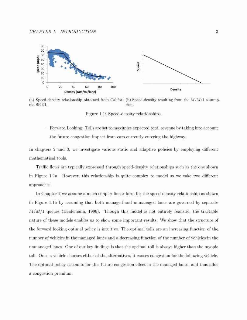
Figure 1.1: Speed-density relationships.
– Forward Looking: Tolls are set to maximize expected total revenue by taking into account
the future congestion impact from cars currently entering the highway.
In chapters 2 and 3, we investigate various static and adaptive policies by employing different
mathematical tools.
Traffic flows are typically expressed through speed-density relationships such as the one shown
in Figure 1.1a. However, this relationship is quite complex to model so we take two different
approaches.
In Chapter 2 we assume a much simpler linear form for the speed-density relationship as shown
in Figure 1.1b by assuming that both managed and unmanaged lanes are governed by separate
M/M/1 queues (Heidemann, 1996). Though this model is not entirely realistic, the tractable
nature of these models enables us to show some important results. We show that the structure of
the forward looking optimal policy is intuitive. The optimal tolls are an increasing function of the
number of vehicles in the managed lanes and a decreasing function of the number of vehicles in the
unmanaged lanes. One of our key findings is that the optimal toll is always higher than the myopic
toll. Once a vehicle chooses either of the alternatives, it causes congestion for the following vehicle.
The optimal policy accounts for this future congestion effect in the managed lanes, and thus adds
a congestion premium.

CHAPTER 1. INTRODUCTION 4
Our numerical experiments show that both myopic and static policies fall well short of generating
maximum revenue. This shows that the operator can achieve a significant amount of revenue
improvement by adjusting the fees in real-time according to current conditions. Another important
insight we get is regarding investments in managed lanes. In our experiments we saw that in heavily
congested systems even a small level of capacity in the priced queue (managed lanes) is enough to
reap most of the financial benefits.
Furthermore, in the case of a time-varying traffic load, the revenue-maximizing toll at any time
strongly depends on anticipated future demand. In particular, for the same current state, the
optimal forward looking tolls are generally higher when arrival intensity is forecast to increase than
when arrival intensity is forecast to decrease. The intuition behind this result is that the optimal
toll not only generates immediate revenue, it also channels users into the unmanaged lanes. When
traffic is high and increasing (say entering a morning peak), it is profitable to use a higher fee to
“steer” arriving vehicles to the unmanaged lanes. This increases congestion in the unmanaged lanes
for some period, which allows higher tolls to be charged in the future. If, on the other hand, arrival
intensity is decreasing (or is very low), steering additional vehicles to the unmanaged lanes will not
result in much increased congestion in those lanes. In this case, the optimal policy comes closer to
maximizing the expected revenue from each arriving vehicle (the myopic policy). A key managerial
insight is that incorporating expectations of future arrivals into the determination of the current
toll is critical if the goal is revenue maximization.
There is a close relationship between this chapter and the literature on pricing for queueing
systems with time-sensitive customers. Hassin and Haviv (2003) provide an excellent survey of this
literature. We analyze static policies as in Naor (1969) and also dynamic policies like Low (1974).
Unlike Chapter 2, none of the existing work in this area consider dynamic pricing under the presence
of multiple competing queueing systems and they do not consider non-homogeneous arrivals. Some
work has also been done on the design of joint price and service-level menus for queueing systems. A
notable example is Afeche (2010) who analyzes the design of a revenue-maximizing price/lead-time
product menu for a multi-product M/M/1 queue. The congestion fee concept (difference between
optimal forward looking and myopic tolls) described in the previous paragraphs is very similar in

CHAPTER 1. INTRODUCTION 5
1
Figure 1.2: Constituent modules in the simulator.
flavor to his main finding where he shows that it can be optimal to induce “artificial” delay in one
queue in order to increase the willingness-to-pay of arrivals to join the another queue. However, his
setting is different from ours: we assume that introducing artificial delays are not permitted. How
to cope with the time varying loads in queues has been well studied from a staffing perspective
(Green et al., 2009). However, in this study we keep the staffing fixed, i.e., there is only one server
in each queue, and instead adjust the tolls dynamically over time.
Given the potential benefits surrounding adaptive tolling, we take a more practical viewpoint
of the problem in Chapter 3 by building a simulation that models traffic propagation on a highway
with a high degree of realism. This serves two purposes. First, we develop the methodology that
can be easily used in practice to set revenue maximizing tolls for managed lanes. Second, using
this methodology we analyze and compare the structure and performance of various tolling policies
through a numerical study.
A high level overview of the simulation approach employed in this chapter is shown in Figure
1.2. The highway simulation is time based. In each time increment, the demand generation module
determines how much new traffic arrives to the system. The consumer choice module takes the
current traffic load as an input from the demand generation module. Based on the current toll and
time differential between the managed and unmanaged lanes, it determines the proportions of the
arriving traffic that choose the managed and unmanaged lanes. The highway simulation module
uses that information to update the traffic on the managed and unmanaged lanes. This process
keeps on repeating itself until the stopping time for the simulation is reached. In the numerical
study, we start with an empty highway and simulate the system for a whole day.

CHAPTER 1. INTRODUCTION 6
This chapter provides a number of important insights into optimal managed lane tolling policies.
First of all, managing tolls around peaks – especially entering into the peak – is the most important
aspect of any revenue-maximizing policy. Secondly, optimal tolls have a“jam and harvest”character
– by charging high tolls entering into a peak period, they divert cars into the unmanaged lanes
increasing unmanaged lane congestion and enabling higher tolls later in the peak. These two
observations are similar to the findings obtained in Chapter 2. Specifically, we see that accounting
for the expectations of future arrivals in the current tolls provides substantial value. Finally, when
the peak traffic is high relative to off-peak traffic, good heuristic policies can generate substantially
more revenue than the myopic policy.
During our analysis we found that an adaptive tolling mechanism potentially provides substan-
tial revenue improvements over a static time-of-use policy. We show that such a policy does not
need to be very complex. What counts most is having the capability of sensing whether the traffic
load is higher than usual or not.
In Chapter 4 we look at the revenue management of consumer options for sporting events. We
study the potential revenue improvements of offering options, relative to only offering advance tick-
ets. The World Cup final, the Super Bowl, and the final game of the NCAA Basketball Tournament
in the United States (a.k.a. “March Madness”) are among the most popular sporting events in the
world. Typically, demand exceeds supply for the tickets for these events, even when the tickets cost
hundreds of dollars. However, since these events are the final games of a tournament, the identities
of the two teams who will be facing each other are typically not known until shortly before the
event. For example, the identity of the two teams who faced each other in the 2010 World Cup final
was determined only after the completion of the two semi-final games, five days prior to the final.
Yet, tickets for the World Cup Final are offered for sale many months in advance. While there may
be many fans who are eager to attend the final game no matter who plays, many fans would only
be interested in attending if their favored team, say Germany, were playing in the final. These fans
face a dilemma. If they purchase an advance ticket, and Germany does not advance to the final,
then they have potentially wasted the price of the ticket, especially if there is no secondary market.
On the other hand, tickets are likely to be sold out well before it is known who will be playing in

CHAPTER 1. INTRODUCTION 7
the finals, so if fans wait, they may be unable to attend at all. In response to this dilemma, some
sporting events have begun to offer “ticket options” in which a fan can pay a nonrefundable deposit
up front for the right to purchase a seat later once the identity of the teams playing is known.
Essentially, this is a call option by which the fan can limit his cost should his team not make the
final while guaranteeing a seat if his team does make the final. In this chapter, we address the
revenue management problem faced by the event manager (or promoter) of a tournament final who
has the opportunity to offer options for the final. We examine when it is most profitable to offer
options to consumers and how the manager should set prices and availabilities for both the advance
tickets and the options. We also address the social welfare implications of offering options.
Over the past five years, a number of events and third-parties have begun to offer call options
for sporting event tickets. For example, the Rose Bowl is an annual post-season event in which
two American college football teams are chosen to play against each other based on their records
during the regular season. The identity of the teams playing is not known until a few weeks prior
to the event, however, the Rose Bowl sells tickets many months in advance. In addition to general
“advance tickets”, the Rose Bowl also sells “Team Specific Reservations”. As described on the Rose
Bowl’s web-site 2:
TeamTix are team specific reservations for the right and obligation to purchase a
face value ticket, if and only if your team qualifies to play in the game. The price of the
face value ticket(s) is an amount you pay that is over and above the amount you pay
for the TeamTix, if your team qualifies for the game.
In addition to the Rose Bowl, at least one web site, www.OptionIT.com offers options for a variety
of sporting events.
While options can be offered for any sporting event, in this chapter we consider only the case
of tournament options, which are sold for a future event in which the two opponents who will face
each other are ex-ante unknown. We assume that there are potential customers – “fans” – whose
utility of attending the game is dependent upon whether or not their favored team is playing. In
2http://bcschampionship.teamtix.com/content/home

CHAPTER 1. INTRODUCTION 8
this case, the tournament option enables a fan to hedge against the possibility that his favored
team is not selected to play in the game of interest – e.g. the World Cup final.
This chapter addresses a particular case of the classic revenue management problem of pricing
and managing constrained capacity to maximize expected revenue in the face of uncertain demand.
Overviews of revenue management can be found in Talluri and van Ryzin (2004) and Phillips (2005).
While the revenue management literature is vast, there has been relatively little research on its
applications to sporting events. Barlow (2000) discusses the application of revenue management to
Birmingham FC, an English Premier League soccer team. Chapter 5 of Phillips (2005) discusses
some pricing approaches used by baseball teams and Phillips et al. (2006) describe a software system
for revenue management applicable to sporting events. Duran et al. (2011) and Drake et al. (2008)
consider the optimal time to switch from offering bundles (e.g. season tickets) to individual tickets
for sports and entertainment industries. None of these works address the use of options.
Research specifically on the use of options for sports events is very scarce. The first attempt to
analyze such options was by Sainam et al. (2009). The authors devise a simple analytical model to
evaluate the benefits of offering options to sports event organizers. They show that organizers can
potentially increase their profits by offering options to consumers in addition to advance tickets.
They also conduct a small numerical study to support their theoretical findings. However, they do
not address the problem of pricing options or determining the number of tickets to sell.
In the absence of discounting, a consumer call option for a future service is equivalent to a
partially refundable ticket. Gallego and Sahin (2010) show how such partially refundable tickets
can increase revenue relative to either fully refundable or non-refundable tickets and that they can be
used to allocate the surplus between consumers and capacity providers. They show that offering an
option wherein an initial payment gives the option of purchasing a service for an additional payment
at a later date can provide additional revenue for sellers. Gallego and Stefanescu (2012) discuss
this as one of several “service engineering” approaches that sellers can use to increase profitability.
The same result holds for a consumer call option in the case when the identity of the teams is
known ex-ante. Our work extends their work by incorporating the correlation structure on ex-post
customer utilities imposed by the structure of the tournament.

CHAPTER 1. INTRODUCTION 9
We propose a demand model where consumers are segmented by their preferred teams. We
do not enforce any a priori segmentation across products. Instead, we postulate a neoclassical,
risk-neutral, choice model where consumers maximize their expected surpluses. We allow fans to
choose which product to purchase based on (i) prices, (ii) product availability, (iii) their intrinsic
willingness-to-pay, and (iv) their rational expectations about the likelihood of the different out-
comes. Thus, in our model, the demands for products are not independent, and a price-sensitive
consumer choice model naturally arises.
In order to capture fans’ sensitivity to the teams playing in the final game, we introduce a
parameter termed love-of-the-game that measures the value to a fan of attending a game in which
their favorite team does not play. The higher the value of this parameter, the more utility that fans
derive from a game in which their favorite team is not playing. This parameter turns out to be
critical in our model, and strongly influences the profitability of introducing options. Estimation of
the fans’ willingness-to-pay and their sensitivity to the teams playing in the final could be estimated,
for example, with an empirical study similar to the one of Sainam et al. (2009) who estimated the
willingness to pay of consumers for advance tickets and options under various probabilities of their
favorite team playing in a final.
We address the joint problem of pricing and capacity allocation. We assume the event manager
announces ticket prices at the beginning, and these remain fixed throughout the sales horizon.
However, as demand realizes, the manager can control ticket sales by dynamically managing the
availability of products. The sequential nature of these decisions suggests a two-stage optimization
problem: set prices in the first stage, and allocate capacity given the fixed prices in the second
stage. The capacity allocation problem in the second stage is a continuous time stochastic control
problem under a discrete choice model, which in most real world applications can not be efficiently
solved to optimality.
Different methods have been proposed in the literature to solve the capacity allocation problem.
For example, Zhang and Adelman (2006) proposed an approximate dynamic programming approach
in which the value function is approximated with an affine function of the state vector. Another
popular approach, which we adopt here, considers a deterministic approximation of the capacity
CHAPTER 1. INTRODUCTION 10
allocation problem, in which random variables are replaced by their means and products are allowed
to be sold in fractional amounts (Gallego et al., 2004). The deterministic approximation results in a
linear program. Unfortunately, the resulting LP grows exponentially with the number of teams. One
of our contributions is an approximation that only grows quadratically with the number of teams.
This allows us to efficiently solve instances of moderate size jointly on prices and capacity allocation.
Additionally, we give precise bounds for the performance of that deterministic approximation and
show that it is asymptotically optimal for the stochastic problem.
To provide some insight we analyze the symmetric problem, i.e., the case in which all teams
have the same probability of reaching the final and the fans of all teams share the same valuations
and love-of-the game. These simplifying assumptions allow us to characterize the conditions under
which offering options is beneficial to the event manager. Though not entirely realistic, this analysis
provides simple rules of thumb that can be applied to the general case. Specifically, we show that
options are beneficial for the event manager only when the demand is high with respect to the
stadium’s capacity and fans strictly prefer their own team over any other. Additionally, we show
that the value to the event manager of offering options decreases as the love-of-the-game parameter
increases. That is, as fans become more averse to seeing other teams play, options become more
attractive to them, and the event manager can take advantage of this by offering options. We
also show that, under some mild assumptions, the introduction of options increases the consumer’s
surplus. This should not be surprising because options allow fans to hedge against the risk of
watching a team that it is not of their preference. Lastly, we explore the idea of full-information
pricing where the event manager prices the tickets after the finalists are determined, and show that
offering options is a better strategy.
In the last chapter, we analyze infrastructure investments. In many industries, the historical
trend is toward ever increasing unit size of technology. By unit size we mean the capacity of a single
unit of technology, e.g., the number of people carried by a single aircraft, load capacity of a single
mining truck, the watts of electric power produced by a single generator, etc. Food, once produced
on small family plots, now comes overwhelmingly from industrial factory farms. Ships that in the
early twentieth century carried 2,000 tons of cargo have been replaced by modern container ships

CHAPTER 1. INTRODUCTION 11
that routinely move 150,000 tons. Coal-fired power plants that averaged 50 MW of output in 1950
today approach 1 GW. The list goes on.
What underlies the trend of “bigger is better?” Before exploring this question further, we need
to distinguish between the traditional notion of economies of scale, which encompasses all possible
benefits associated with increasing total firm-wide output, and those benefits that are directly
attributable to building and operating larger individual units of technology. Here we are interested
in the latter, which we refer to as economies of unit scale.
While the development of ever larger unit size may have made sense historically, we submit
that the incentives today for continuing the trend are less compelling - and indeed there may be
tremendous benefit in reversing it. It is now realistic to consider a radically new approach to
infrastructure design, one that replaces economies of unit scale with economies of numbers; that
phases out custom-built, large-unit-scale installations and replaces them with large numbers of
mass-produced, modular, small-unit-scale technology – operated in either centralized or distributed
fashion – offering new possibilities for reducing cost and improving service. In the context of
electricity generation, some of these concepts are reflected in the “Small Is Profitable” work of
Lovins et al. (2002), but the idea applies much more broadly.
The total lifecycle cost of a unit can be divided into two parts: capital and operating costs. In
this chapter we demonstrate that in many industries there is close to parity between small modular
units and larger conventional units for both of these costs.
Specifically, we show that modern mass production of many small standardized units can achieve
capital cost saving comparable to, or even larger than those achievable through large unit scale.
For instance, a mass produced car engine costs $10/kW, while a typical large-scale fossil fuel fired
power plant costs about $1000/kW (Larminie and Dick, 2003; EIA, 2010b). Since operating labor
cost alone rendered small unit scale technology uneconomical in the past, there was little incentive
to pursue the possibility of mass-produced capital; today, that situation is fundamentally altered.
Operating costs can be roughly divided into labor and fuel costs. We argue that technologies
for automating processes exist today that were previously unavailable. In the past, a massively
modular approach to infrastructure was simply infeasible because of excessive personnel cost. To-

CHAPTER 1. INTRODUCTION 12
day however, current computing, sensor and communication technologies make high degrees of
automation possible at very low cost, radically undercutting the logic that significant labor savings
can only be obtained through large unit scale. Through the use of several examples, we show that
as the unit size gets larger and larger conversion efficiency of a unit does not necessarily increase
significantly. As a result, for many industries, we demonstrate that the operating costs of large and
small units are comparable to each other.
Lastly, there are many inherent flexibility benefits to small unit scale, which in the past have
largely been ignored. Small-scale units can be used in multiples to better match the output re-
quirements of a given project and can also be deployed gradually over time, both of which reduce
investment cost and risk. They offer geographic flexibility; multiple small units can be aggregated
at a single location to achieve economies of centralization (e.g. to reduce overhead or transport
costs) or they can be distributed to be closer to either sources of supply or points of demand.
Small unit scale also offers flexibility in output; having many units of small scale makes it possible
to selectively operate varying numbers of units to better match short-run variations in demand.
Also, one can achieve high reliability through enormous redundancy and statistical economies of
numbers.
Since larger units no longer dominate smaller units from a capital and operating cost standpoint,
the added flexibility benefits from smaller units suggest that not every industry requires large units
to be cost-effective. We end the chapter by analyzing several industries where we believe a shift
towards smaller unit sizes will introduce significant cost savings.
CHAPTER 2. ANALYSIS OF PRICING MANAGED LANES USING QUEUEING SYSTEMS13
Chapter 2
Analysis of Pricing Managed Lanes
Using Queueing Systems
This chapter deals with an important part of infrastructure systems, namely, transportation. We
specifically focus on the pricing of managed lanes. Utilizing a simple queueing based model, we
analyze the revenue maximizing tolling strategies for managed lanes. We pay particular attention
to policies where the system operator has the flexibility to adjust the toll according to real time
traffic conditions. Our analysis focuses on the characteristics of such policies and the potential
revenue improvements that they can provide.
2.1 Model
We assume that both unmanaged and managed lanes are governed by different M/M/1 queues.
The service rates of queues corresponding to both lanes are fixed and denoted by µi for i = u,m.
Traffic arrives according to a Poisson process with rate λ. For stability, we assume that λ is strictly
less than both µu and µm. The time-varying toll of the managed lane is denoted by p(t), and the
operator is subject to the nonnegative toll constraint p(t) ≥ 0. The state of the system at time t
is given by the vector x(t) = (xu(t), xm(t)), where xm(t) and xu(t) denote the number of cars in
the managed and unmanaged lanes, respectively. From this point on, bold characters will denote
CHAPTER 2. ANALYSIS OF PRICING MANAGED LANES USING QUEUEING SYSTEMS14
two-dimensional vectors. Given the state of the system x(t), ∆T (x(t)) denotes the expected time
savings an arriving vehicle can realize by choosing the managed lane,
∆T (x(t)) =xu(t) + 1
µu− xm(t) + 1
µm.
When ∆T (x(t)) > 0, there are expected time savings from choosing the managed lanes.
We utilize a standard random utility model in which there is some distribution of “value-of-
time” among drivers. We denote the value-of-time of a driver with V . Let F be the cumulative
distribution function of this random valuation and F denote 1 − F . We assume that the p.d.f. f
is continuously differentiable, has support [0, v] for some v ∈ (0,∞), and the valuations are i.i.d.
across drivers. We will assume that the operator knows the distribution F but the individual value
of each driver is private.
An arriving driver chooses the managed lanes if and only if V∆T (x(t)) ≥ p(t). So, the corre-
sponding probability that an arriving car chooses the managed lanes is F(
p(t)∆T (x(t))
). If the expected
time it takes to traverse both lanes is equal and the toll is zero, then we assume that an motorist
will choose one of the lanes with equal probability. In all other cases the managed lane arrival rate
will be zero. With some abuse of notation, let λm(x(t), p(t)) denote the arrival rate to the managed
lane at time t which has the following structure
λm(x(t), p(t)) =
λF(
p(t)∆T (x(t))
)if ∆T (x(t)) > 0,
λ/2 if ∆T (x(t)) = 0 and p(t) = 0,
0 o.w.
Given a state x, the toll operator is subject to the following control set
U(x) =
p|0 ≤ p ≤ v∆T (x) if ∆T (x) > 0,
0, p if ∆T (x) = 0,
0 o.w.

CHAPTER 2. ANALYSIS OF PRICING MANAGED LANES USING QUEUEING SYSTEMS15
When there are time savings, the operator can set his price as high as v∆T (x) which ensures that
an arriving car chooses the unmanaged lanes. If there are no time savings, then the operator is
faced with two choices. He can either set the toll to zero so that vehicles choose both lanes with
equal probability, or he can set the toll to any positive scalar and an arriving vehicle will choose the
unmanaged lanes. Lastly, if there are no time savings from taking the managed lanes, the operator
sets the toll to either zero or some arbitrary positive toll p.
In the next two sections, we explore the revenue maximization problem from two perspectives.
First, we look at the expected discounted revenue, and then we analyze the average revenue max-
imization problem. In both cases we first formulate the problem using continuous time Markov
chains. Afterwards, using a uniformization procedure we convert the problems into discrete time
dynamic programs. Using the dynamic programs we obtain, we explore the structural properties of
the optimal dynamic tolling policy. The last section extends the results to the case of non-stationary
arrival rates.
2.1.1 Discounted Revenue Case
Let us start by writing down the discounted revenue case in the continuous time Markov chain
(CTMC) framework. Our aim is to maximize the expected discounted revenue,
limT→∞
E
[∫ T
0e−βtλm(x(t), p(t))p(t)dt
], (2.1)
where β > 0 is the continuous discount rate.
Next, we show how we can obtain an optimal dynamic pricing policy for (2.1) using dynamic
programming. The process x(t) is a continuous time Markov chain and the total transition rate
out of any state is bounded by ν = λ+µu+µm. Thus, we convert this problem into a discrete-time
infinite horizon discounted dynamic programming problem by using uniformization. We also drop
the time notation (Bertsekas 2007). The optimal discounted revenue when the initial state is x,
CHAPTER 2. ANALYSIS OF PRICING MANAGED LANES USING QUEUEING SYSTEMS16
denoted by J(x) satisfies the Bellman equation
J(x) =
(ν
β + ν
)maxp∈U(x)
[(λm(x, p)
ν
)(p+ J(x + e2)) +
(λ− λm(x, p)
ν
)J(x + e1) (2.2)
+µuνJ(x− e1)+ +
µmνJ(x− e2)+
],
where ei denotes the ith unit vector, and for x ∈ S, we have x+ = (maxx1, 0,maxx2, 0).
The state space of this dynamic program is S = x ∈ N0 ×N0, and ν/(β + ν) < 1 is the discount
factor. The expected revenue in a period is r(x, p) = λm(x, p)p/(β + ν). By cancelling out the
common terms, we can express the DP in (2.2) as
J(x) =1
β + νmaxp∈U(x)
[λm(x, p)(p+ J(x + e2)) + (λ− λm(x, p))J(x + e1) (2.3)
+ µuJ(x− e1)+ + µmJ(x− e2)+].
In general, showing the existence of an optimal stationary policy for an infinite horizon dis-
counted DP is straightforward when the per period reward is uniformly bounded on the state space.
However, for the DP in (2.3) that is not the case. Furthermore, the existence of a value function
J∗ that satisfies the Bellman equation is not guaranteed. Using the next theorem we establish the
existence of both an optimal stationary policy and a solution to the Bellman equation.
Theorem 1. Assume that an arbitrary positive real-valued function w defined on S, and positive
scalars α and L exist that satisfy,
1. infx∈S w(x) > 0,
2. supp∈U(x) |r(x, p)| ≤ αw(x),
3.∑
j∈S qπ(j|x)w(j) ≤ w(x) + L ∀p ∈ U(x),∀x ∈ S, where qπ(j|x) denotes the probability of
transitioning from state x to j under any arbitrary feasible policy π.
Then, a unique solution J∗ exists for the optimality equation given in (2.3) that is obtainable through
value iteration. Furthermore, an optimal stationary policy pd exists for the DP.

CHAPTER 2. ANALYSIS OF PRICING MANAGED LANES USING QUEUEING SYSTEMS17
Proof: See Theorem 6.10.4 and Proposition 6.10.5 in Puterman (1994).
Proposition 1. For w(x) = max (∆T (x), 1), α = v and L = max(
1µu, 1µm
), all three conditions
in Theorem 1 are satisfied.
Proof: Condition 1 is satisfied by the definition of w. Now, we show that Condition 2 is also
satisfied. We separate the state space into two disjoint sets: S1 = x ∈ S|∆T (x) ≤ 0 and
S2 = S \ S1. S1 is the set of states for which taking the managed lanes provides no time savings,
and S2 contains the states for which taking the managed lanes provides time savings. For x ∈ S1,
we have r(x, p) = 0 and Condition 2 is satisfied. When x ∈ S2, we have
r(x, p) =
(λ
β + ν
)F
(p
∆T (x)
)p ≤ v∆T (x) ≤ vw(x). (2.4)
The inequality comes from the fact that λ/(β + ν) < 1, F is bounded by one, and p ∈ [0, v∆T (x)].
So, Condition 2 is satisfied for this case as well.
Next, we show that Condition 3 is satisfied. First, note the following inequalities
w(x + e1) ≤ w(x) +1
µu,
w(x− e1) ≤ w(x),
w(x + e2) ≤ w(x),
w(x− e2) ≤ w(x) +1
µm.
Using the above inequalities we get
∑j∈S
qπ(j|x)w(j) ≤ w(x) + max
(1
µu,
1
µm
),
for any arbitrary feasible policy π, and x ∈ S. Thus, we can see that the last condition is also
satisfied.
CHAPTER 2. ANALYSIS OF PRICING MANAGED LANES USING QUEUEING SYSTEMS18
In addition to showing the existence of a unique solution to the Bellman equation in (2.3),
Proposition 1 showed it can be obtained through a value iteration procedure. In the context of our
problem, such a procedure iterates over
Jk+1(x) =
(1
β + ν
)maxp∈U(x)
[λm(x, p)(p+ Jk(x + e2)) + (λ− λm(x, p))Jk(x + e1)
+ µuJk(x− e1)+ + µmJk(x− e2)+],
where J0(x) = 0. Jk is also called the k-stage problem since it is a finite horizon dynamic program
with k stages. The convergence of the value iteration procedure implies that limk→∞ Jk(x) = J∗(x).
Proposition 2. For all x ∈ S, J∗(x) ≤ v(β+ν)β
(w(x) + Lν
β
).
Proof: We start by proving that for any arbitrary feasible policy (possibly nonstationary) π and
x ∈ S we have,
Eπ(r(xn, πn)|x0 = x) ≤ v(∆T (x) + nL), (2.5)
where xn, πn denote the state and action taken in period n, and Eπ denotes the expectation operator
under the policy π. We proceed by induction. It is easy to see that the case n = 1 holds. Now,
assume the claim holds for n = k − 1. Then,
Eπ[r(xk, πk)|x0 = x] =∑y∈S
qkπ(y|x)r(y, πk),
=∑y∈S
∑z∈S
qk−1π (z|x)qπ(y|z)r(y, πk),
=∑z∈S
qk−1π (z|x)
∑y∈S
qπ(y|z)r(y, πk),
≤∑z∈S
qk−1π (z|x)
∑y∈S
qπ(y|z)vw(y),
≤ v∑z∈S
qk−1π (z|x)(w(z) + L),
≤ v(w(x) + kL),

CHAPTER 2. ANALYSIS OF PRICING MANAGED LANES USING QUEUEING SYSTEMS19
where the interchange of summations is justified since all terms are nonnegative. The first inequality
above comes from (2.4), the second comes from the base case, and the last from the induction
assumption.
We now use (2.5) to show that the value function is bounded for every x ∈ S.
J∗(x) =∞∑n=0
(ν
β + ν
)nEpd [r(xn, pd)|x0 = x],
≤ v∞∑n=0
(ν
β + ν
)n(w(x) + nL),
=v(β + ν)
β
(w(x) +
Lν
β
).
The bound established in Proposition 2 is linear with respect to the number of cars in the system.
Specifically, the bound is increasing (decreasing) in the number of cars in the unmanaged (managed)
lanes. This suggests that J∗ might be a monotonic function and Proposition 3 establishes that is
correct. It states that the value function actually moves in the same direction as its bound with
respect to the number of cars in the system. This result is intuitive since as the unmanaged lanes
get relatively more congested, the attractiveness of the managed lanes increases and the operator
can charge a higher toll. On the other hand, as the managed lanes start to lose their attractiveness,
the operator starts to charge a higher toll and the revenue potential decreases.
Proposition 3. For all x ∈ S, we have J∗(x + e1) ≥ J∗(x) and J∗(x + e2) ≤ J∗(x).
Proof: We use a coupling argument. Consider a k-stage problem with a terminal reward function
J0(x) = 0 for all x ∈ S. We consider two different systems A and B starting from two different
initial states x and x + e1, respectively. By defining the systems on a common probability space,
we can assume that for both A and B arrivals and departures happen at same points in time. We
assume that System A follows the optimal policy pd, and System B sets its toll such that at any
time its probability of admitting a car into the managed lane is the same as System A. As a result,
the toll that System B will be charging is always greater than or equal to the toll that System A

CHAPTER 2. ANALYSIS OF PRICING MANAGED LANES USING QUEUEING SYSTEMS20
will be charging. So, the revenue stream generated by System B will be greater than or equal to the
revenue stream generated by System A. Furthermore, the revenue generated by System B operated
under this policy is less than or equal to the optimal. So, we get the following
Jk(x + e1)− Jk(x) ≥ 0. (2.6)
Since the convergence of the value iteration algorithm has already been established in Proposi-
tion 1, we take the limit as k →∞ in (2.6) to conclude
J∗(x + e1)− J∗(x) ≥ 0.
This proves the first part of the proposition. The proof for the second part is similar and thus
omitted.
Next, we show the following simple corollary that will come in handy later.
Corollary 1. For all x ∈ S, ∆J∗(x) = J∗(x + e1)− J∗(x + e2) ≥ 0.
Proof:
∆J∗(x) = J∗(x + e1)− J∗(x + e2),
= J∗(x + e1)− J∗(x) + J∗(x)− J∗(x + e2),
≥ 0,
where the inequality comes from Proposition 3.
We have showed the monotonicity of the value function in Proposition 3. However, it does not
tell us anything about how fast the value function increases or decreases. In the next proposition
we show that the speed is bounded.
Proposition 4. For all x ∈ S, J∗(x + ke1) − J∗(x) ≤ vν(xu+k)2
µu(µu−λ) , and J∗(x) − J∗(x + ke2) ≤

CHAPTER 2. ANALYSIS OF PRICING MANAGED LANES USING QUEUEING SYSTEMS21
(v(xm+k)µm
) [ν(xuµu
)+ λ+ µu
].
Proof: Similar to the proof of Proposition 3, we use a coupling argument. Let us start with the first
part of the proposition. Consider two systems, A and A′, that are defined on a common probability
space and start from the same state x + ke1. System A′ is a modification to A defined as follows.
Until some stopping time τ is reached, A′ earns r′(x) = v∆T (x) every period which is greater than
the revenue rate of A for any policy. Once the stopping time τ is reached, then the revenue rate
of A′ is replaced with the original r(.). So, for any policy p1, p2, . . . and stopping time τ we have
the following,
E
( ∞∑t=0
(ν
β + ν
)tr(xt, pt)
∣∣∣∣∣x0 = x + ke1
)≤ E
(τ−1∑t=0
(ν
β + ν
)tr′(xt)
+
(ν
β + ν
)τJ(xτ )
∣∣∣∣x0 = x + ke1
), (2.7)
where xt is a vector denoting the number of cars in the system at the beginning of each period.
Now, let us define τ as the first time the number of cars in the unmanaged lanes hits zero. Note
that P (τ <∞) = 1 for any policy since λ < µu. When A follows the optimal policy, the left hand
side of (2.7) becomes equal to J(x + ke1). The policy that maximizes the right hand side of (2.7)
is the one that directs all arrivals into the unmanaged lanes since it maximizes the period of time
that passes before the revenue rate function is replaced with the original one. Furthermore, for
any given sequence of events, it leaves the system in the best possible state, i.e. the state with the
highest expected discounted revenue. Then we have,
J∗(x + ke1) ≤ E
(τ−1∑t=1
(ν
β + ν
)tr′(xt) +
(ν
β + ν
)τJ(xτ )
∣∣∣∣∣x1 = x + ke1
). (2.8)
Now, we define a second system B that is defined on the same probability space as A and
A′. Assume that B directs all arrivals into the unmanaged lanes until the number of cars in the
unmanaged lanes of A′ hits zero. Thus, the actual arrivals and departures from both systems are
the same and they are found in the same state when the stopping time τ is reached. Clearly, this

CHAPTER 2. ANALYSIS OF PRICING MANAGED LANES USING QUEUEING SYSTEMS22
is a suboptimal policy for B and we have,
J∗(x) ≥ E((
ν
β + ν
)τJ(xτ )
∣∣∣∣x1 = x + ke1
). (2.9)
Let yt denote the change in the number of cars in the unmanaged lanes from period t− 1 to t
for the policy used in A′ and B. Then, yt has the following distribution,
yt =
1 w.p. λ/ν,
0 w.p. µm/ν,
−1 w.p. µu/ν.
We make a few observations before proceeding with the remainder of the proof. Note that
E (∑τ
t=1 yt) = −(xu + k) by the definition of stopping time τ , and from Wald’s Equation E(τ) =
E (∑τ
t=1 yt) /E(yt) = (xu + k)ν/(µu − λ) (Ross, 1996). Combining this observation with (2.8) and
(2.9) we get,
J∗(x + ke1)− J∗(x) ≤ E
(τ−1∑t=0
(ν
β + ν
)tr′(xt)
∣∣∣∣∣x0 = x + ke1
),
≤ E
(τ∑t=0
r′(xt)
∣∣∣∣∣x0 = x + ke1
),
≤ E
(τ∑t=0
v
(xu,tµu
)∣∣∣∣∣x0 = x + ke1
),
= v
[E
(τ∑t=0
xu + k
µu
)+ E
(τ∑t=1
ytµu
)],
= v
[(E(τ) + 1)
(xu + k
µu
)−(xu + k
µu
)],
=vν(xu + k)2
µu(µu − λ),
where the second inequality comes from the nonnegativity of r′ and ν/(β + ν) < 1, the third from
r′(xt) ≤ xu,t/µu since xu,t ≥ 0 for 0 ≤ t ≤ τ , and the last inequality follows from Wald’s Equation.
The second part of the proposition is proven similarly. Systems A and B now start from x and

CHAPTER 2. ANALYSIS OF PRICING MANAGED LANES USING QUEUEING SYSTEMS23
x + ke2, respectively. System B is operated under the suboptimal policy of directing all the cars
into the unmanaged lanes. Now, the stopping time τ is defined as the first time the number of cars
in the managed lanes of B is equal to zero, and E(τ) = xmν/µm. Unlike the previous case, note
that now τ is dependent on the state of System B. Again, A′ starts from x with r′ as the revenue
rate which is replaced with the original at τ . The optimal policy for A′ is still to direct all arriving
cars into the unmanaged lanes. Note that the expected revenue from A′ is still an upper bound
for the expected revenue from A that is operated optimally. Furthermore, systems A′ and B are
found in the same state at time τ . Let zt denote the absolute change in the number of cars in the
unmanaged lanes from period t− 1 to t for the policy used in A′ and B,
zt =
1 w.p. (λ+ µu)/ν,
0 w.p. µm/ν.
(2.10)
So, we have
J∗(x)− J∗(x + ke2) ≤ E
(τ∑t=1
r′(xt)
∣∣∣∣∣x1 = x
),
≤ v
[E
(τ∑t=1
xu + k
µu
)+ E
(τ∑t=1
ztµu
)],
=
(v(xm + k)
µm
)[ν
(xuµu
)+ λ+ µu
],
where the first inequality comes from the first part of the proof, the second from r′(xt) ≤ (xu,t +
zt/µu), and the equality from Wald’s Equation.
Continuing with our results about the structure of the value function, we now show that it is
convex nondecreasing (concave nonincreasing) with the number of cars in the unmanaged (managed)
lanes. It worth pointing out that this result is independent of the distribution of V . Furthermore,
this result will play an important role in establishing the structure of the optimal tolling policy.
Proposition 5. For x ∈ S, J∗(x) is convex in xu and concave in xm.

CHAPTER 2. ANALYSIS OF PRICING MANAGED LANES USING QUEUEING SYSTEMS24
Proof: We show the convexity of J∗ in xu by induction on the k-stage problem Jk(x) with the
boundary Condition J0(x) = 0. Note that given a state x, such that ∆T (x) > 0, we have,
p(x, λm) = ∆T (x)F−1
(λmλ
).
With some abuse of notation, let r(x, λm) denote the expected revenue as a function of the managed
lanes arrival rate rather than the toll, then
r(x, λm) =
0 if ∆T (x) ≤ 0,(
1β+ν
)∆T (x)F−1
(λmλ
)if ∆T (x) > 0.
Note that for any distribution F and λm ∈ [0, λ], r(x, λm) is convex in xu. Therefore, the base case
k = 1 holds. Assume that Jk(x) is convex for all x ∈ S. In writing Jk+1(x) we treat λm as the
decision variable, and we get
Jk+1(x) =1
β + vmax
λm∈λ(x)[λmp(x, λm) + λmJk(x + e2)) + (λ− λm)Jk(x + e1))
+ µuJk(x− e1)+ + µmJk(x− e2)+],
where λ(x) denotes the set of feasible managed lanes arrival rates for state x. For fixed λm, each of
the elements in the expression being maximized above is convex in xu by the induction assumption
and the convexity of r(x, λm). Thus, the expression being maximized is convex since it is the
nonnegative weighted sum of convex functions. We know that the maximum of convex functions is
also convex (Boyd and Vandenberghe, 2004). Thus, Jk+1(x) is convex in xu and we have
Jk+1(x + e1)− Jk+1(x) ≥ Jk+1(x)− Jk+1(x− e1)+. (2.11)
By taking the limit as k →∞ in (2.11) we get
J∗(x + e1)− J∗(x) ≥ J∗(x)− J∗(x− e1)+.

CHAPTER 2. ANALYSIS OF PRICING MANAGED LANES USING QUEUEING SYSTEMS25
The proof of concavity in xm is similar and thus omitted.
Corollary 2. ∆J∗(x) is nondecreasing in xu and nonincreasing in xm.
Proof: We start by showing that ∆J(x) is nondecreasing in xu. Let us start by noting the following
J∗(x + 2e1)− J∗(x + e1) ≥ J∗(x + e1)− J∗(x),
J∗(x + e1 + e2)− J∗(x + e2) ≤ J∗(x + e1)− J∗(x),
where the first inequality comes from the convexity of J∗ in xu and the latter from its concavity in
xm. By combining these two we get
J∗(x + 2e1)− J∗(x + e1) ≥ J∗(x + e1 + e2)− J∗(x + e2),
J∗(x + 2e1)− J∗(x + e1 + e2) ≥ J∗(x + e1)− J∗(x + e2).
The proof of the second part is similar and thus omitted.
Given these properties of the value function, we can now start analyzing the structure of the
optimal policy. An important aspect of our model is that the operator does not just try to maximize
the expected revenue from an arriving vehicle. He also takes into account the future congestion
that the vehicles joining the system might cause. For example, if an arriving vehicle joins the
unamanaged lanes, then it increases the congestion for those lanes. This enables the operator to
potentially charge a higher toll to the car that arrives next. An interesting question is how would
the operator set the toll if he didn’t take into account that congestion effect? That is, what if he
set the tolls myopically to maximize revenue from each vehicle? What is the relationship between
myopic tolls and optimal tolls? The myopic toll for state x ∈ S is defined as
pm(x) := argmax p∈U(x)λm(x, p)p.

CHAPTER 2. ANALYSIS OF PRICING MANAGED LANES USING QUEUEING SYSTEMS26
Proposition 6. Define S− = x ∈ S|∆T (x) < 0, S0 = x ∈ S|∆T (x) = 0 and S+ = x ∈
S|∆T (x) > 0. The optimal and myopic policies have the following properties:
1. For x ∈ S0, pd(x) = p.
For the remainder, assume V satisfies IFR. Let h(.) denote the hazard rate of V and k be the unique
solution of k = 1/h(k).
2. The optimal stationary policy is unique and strictly monotonic for x ∈ S+. Specifically, the
optimal toll increases as the number of cars in the unmanaged lanes increases and decreases
if the number of cars in the managed lanes decreases.
3. For x ∈ S+, the myopic toll is unique and satisfies pm(x)/∆T (x) = k.
4. For x ∈ S, pd(x) ≥ pm(x).
Proof: Let us start with proving the first claim. For x ∈ S0, the revenue rate λm(x, p)p is zero
regardless of the action that the operator takes. Thus, we can omit that term and rearrange the
right hand side of (2.3) as follows,
J∗(x) =1
β + vmaxp∈U(x)
[−λm(x, p)∆J∗(x) + λJ∗(x + e1) + µuJ∗(x− e1)+ + µmJ
∗(x− e2)+]
Since we have ∆J∗(x) ≥ 0 from Corollary 1, the operator sets pd(x) = p > 0 so that λm(x, p) = 0.
We now proceed with the proof of the second claim. For S− the optimal policy is unique by
the definition of U(x), and for S0 the uniqueness of the optimal policy was shown above. What
remains is to show uniqueness for S+. For an interior solution, the first order condition for the
optimal toll is,
pm(x) = ∆T (x)F(pm(x)∆T (x)
)f(pm(x)∆T (x)
) + ∆J∗(x),
pm(x)
∆T (x)=
1
h(
p(x)∆T (x)
) + ∆J∗(x). (2.12)

CHAPTER 2. ANALYSIS OF PRICING MANAGED LANES USING QUEUEING SYSTEMS27
Since V is IFR, h is strictly decreasing in p and there exists a unique solution to (2.12). Now that
we have shown the uniqueness of the optimal stationary policy, let us show that it is monotonic.
First, let us define g(x, p) as
g(x, p) = ∆T (x)1
h(
p∆T (x)
) + ∆J∗(x).
So, (2.12) can be expressed as p = g(x, p). Proposition 5 we know that ∆J∗(x) is monotonic in x.
Combined with the IFR assumption, this implies that g(x, p) strictly increases (decreases) in xu
(xm) and decreases in p. Thus, the fixed point for g(x, p) is strictly increasing (decreasing) in xu
(xm), and we have shown that the optimal tolls are strictly monotonic in x.
In order to show the third claim, we analyze the first order conditions for the optimal toll
pm(x) = ∆T (x)F(pm(x)∆T (x)
)f(pm(x)∆T (x)
) ,pm(x)
∆T (x)=
1
h(
p(x)∆T (x)
) . (2.13)
Given that V is IFR and k is the unique fixed point of its inverse hazard rate, pm(x) is unique
and satisfies pm(x)∆T (x) = k. The last claim follows immediately from comparing (2.12) and (2.13), and
noticing the nonnegativity of ∆J∗(x) ≥ 0.
Now, let us analyze the implications of Proposition 6. When the managed lanes are more
crowded than the unmanaged lanes, we already know that the operator cannot influence traffic
with the toll so he just sets it to zero. But what about the case when both lanes have equal
expected travel times? Should the operator set the toll to zero and try to congest the managed
lanes even further hoping that he can charge more to cars coming later? Or is it time to set a
positive toll and start clearing out the managed lanes? The second option is the optimal decision,
that is, the operator should set a positive toll so that no arriving car chooses the managed lanes.
Given that V satisfies IFR, the optimal policy has a simple intuitive structure when there
CHAPTER 2. ANALYSIS OF PRICING MANAGED LANES USING QUEUEING SYSTEMS28
are time savings from choosing the managed lanes. As the expected travel time savings from
choosing the managed lanes increases, the operator should increase the tolls monotonically. Once
the managed lanes become relatively more crowded, the operator should decrease the tolls. The
structure of the myopic tolling policy is similar. We showed that there is a linear relationship
between the expected time savings from choosing the managed lanes and the myopic tolls. This
implies that the the myopic tolls are also strictly monotonic with respect to the number of cars in
the managed and unmanaged lanes. Furthermore, it also implies that the fraction of cars choosing
the managed lanes is not state-dependent and fixed.
We now analyze the relationship between myopic and optimal tolls. When the unmanaged lanes
are faster, both policies set the tolls to zero by the definition of the control set. Unlike the optimal
policy, the myopic policy is indifferent between setting the toll to zero and p when the expected
travel times for both lanes are equal since the revenue rate is zero for both cases. However, the
decision that the myopic policy takes is still important since it effects its future revenue stream. In
the numerical examples we will assume that the myopic policy also sets the toll to p which provides
the highest revenue. When the managed lanes are faster, the optimal toll balances the revenue
that the operator can get from the current car versus the congestion it causes for the following car.
Due to that congestion effect the optimal tolls are always greater than or equal to the myopic tolls.
This implies that the probability of a car choosing the managed lanes will always be lower under
the optimal policy.
2.1.2 Average Revenue Rate Case
In the previous section we analyzed the case of discounted revenues. Next, we look at the problem
of maximizing the revenue rate of the system. The expected long-term average revenue is given by,
limT→∞
1
TE
[∫ T
0λm(x(t), p(t))p(t)dt
]. (2.14)
CHAPTER 2. ANALYSIS OF PRICING MANAGED LANES USING QUEUEING SYSTEMS29
Using the uniformization procedure as described in the previous section, we can express (2.14) as
a discrete-time dynamic program with the Bellman equation
J∗ + h(x) = maxp∈U(x)
[λm(x, p)p+
λm(x, p)
vh(x + e2) +
λ− λm(x, p)
vh(x + e1) (2.15)
+µuvh(x− e1)+ +
µmvh(x− e2)+
].
In the above equation J∗ is the optimal expected revenue per unit time and h(x) is the relative
revenue for state x.
Average revenue dynamic programs suffer from serious pitfalls when the state and action spaces
are not finite. Specifically, there is no guarantee that a unique J∗ that is independent from the
initial state will exist, and even if exists the value iteration algorithm used in the proofs of the
previous section may not converge to it (Bertsekas 2007).
By taking advantage of its structure, we can show that our model does not suffer from these
pitfalls. Specifically, we can show that regardless of the initial state, there exists a unique J∗ and
a bounded relative reward function that satisfies the Bellman equation in (2.15).
Theorem 2. Let J∗β(x) denote the unique solution to the Bellman equation in (2.3) as a function
of both the state x ∈ S and the continuous discount factor β. Also, for a fixed state z ∈ S, let
hβ(x) := J∗β(x)− J∗β(z) for all x ∈ S. Assume that the following conditions are satisfied,
1. For some fixed state z ∈ S the value function J∗β(z) is bounded for all β > 0,
2. There exists nonnegative finite functions L and N defined on S such that −N(x) ≤ hβ(x) ≤
L(x) for all x ∈ S and β > 0,
3.∑
y∈S qπ(y|x)L(y) <∞ ∀x ∈ S,
4. For any feasible stationary policy and initial state x ∈ S,
E(L(xn)|x1 = x) <∞ for n ≥ 2,
CHAPTER 2. ANALYSIS OF PRICING MANAGED LANES USING QUEUEING SYSTEMS30
5. For any feasible stationary policy and initial state x ∈ S,
limn→∞
E(L(xn)|x1 = x)
n= 0,
where xn denotes the state of the system in the nth period. Then, there exists a unique constant
J∗ that is independent of the initial starting state, and a sequence of discount factors βn → 0
such that limn→∞
(βnβn+v
)J∗βn(x) = J∗ for all x ∈ S. Furthermore, there exists a relative revenue
function h∗ that satisfies −N(x) ≤ h∗(x) ≤ L(x) such that the pair (h∗, J∗) satisfies the Bellman
equation in (2.15), and any policy pa that achieves the maximum in the Bellman equation is optimal.
Proof: With the exception of one small technical detail, these assumptions correspond to (H1-H4)
and (H*5) in Sennott (1999). The proof then follows from Theorem 7.4.3 and Proposition 7.7.2
therein1.
Proposition 7.7.2 in Sennott (1999) assumes that the action space for each state is finite which
is not the case here. However, the only reason she does so is to ensure the existence of a sequence
of discount factors βn∞n=1 for which the resulting policies converge uniformly as βn → 02. For our
problem, we can find such a sequence of discount factors as follows. As in the proof of Proposition
5, consider the formulation of the Bellman equation (2.3) where λm is the decision variable. For
all x ∈ S, let λβm(x) denote the optimal flow rate into the managed lanes for a discount factor
of β. Take βn∞n=1 as any arbitrary sequence of discount factors such that βn → 0. Notice that
0 ≤ λβnm (x) ≤ λ, and via Theorem 3.6 of Rudin (1976) we can find a subsequence of βn∞n=1 such
that λβnm (x) converges uniformly as n → ∞. Since there is one-to-one correspondence between
tolls and managed lanes flow rates, the arguments in the proof of Proposition 7.7.2 apply for this
subsequence of βn∞n=1.
Proposition 7. All the conditions in Theorem 2 are satisfied with L(x) = vν(xu+k)2
µu(µu−λ) and N(x) =(vxmµm
)(λ+ µu) for x ∈ S.
1Condition (iv) in Theorem 7.4.3 coincides with our third assumption.
2See Remark 7.7.6 in Sennott (1999) for a detailed discussion of this assumption.

CHAPTER 2. ANALYSIS OF PRICING MANAGED LANES USING QUEUEING SYSTEMS31
Proof: Let us show one by one that each assumption in Theorem 2 is satisfied. Proposition 2
implies that the first assumption is satisfied. To show that the second assumption holds, we set
z = 0, i.e., we choose the state of the system without any cars as the fixed state. Now, let us
analyze the relative revenue function hβ(x). We start by showing that it has a finite upper bound,
hβ(x) = Jβ(x)− Jβ(0),
≤ Jβ(xu, 0)− Jβ(0),
≤ vν(xu + k)2
µu(µu − λ)︸ ︷︷ ︸L(x)
,
where the first inequality follows from Proposition 3, and the last one follows from Proposition 4.
Next, we show the existence of a finite lower bound,
hβ(x) = Jβ(x)− Jβ(0),
≥ Jβ(0, xm)− Jβ(0),
≥ −(vxmµm
)(λ+ µu)︸ ︷︷ ︸
N(x)
,
where the first inequality follows Proposition 3, and the last one follows from Proposition 4. So,
we have verified that the second assumption holds.
The third assumption, ∑yS
qπ(y|x)L(y) <∞ ∀x ∈ S, (2.16)
holds since the number of states that one can transition to from any state x ∈ S is finite.
Next, let us show that the fourth assumption holds. Note that L(x) is increasing in only xu.
Thus, for any stationary policy, after n transitions the number of cars in the unmanaged lanes is at
most xu + n. So, E(L(xn)|x1 = x) ≤ L(x + ne1) <∞ for n ≥ 2, and the fourth assumption holds.
We now argue that the last assumption also holds. Let Eπ denote the expectation operator under
CHAPTER 2. ANALYSIS OF PRICING MANAGED LANES USING QUEUEING SYSTEMS32
a stationary policy π and π denote the policy that directs all incoming traffic into the unmanaged
lanes. Then, for all x ∈ S and any feasible policy π we have,
Eπ(L(xn)|x1 = x) ≤ Eπ(L(xn)|x1 = x). (2.17)
The Markov chain that policy π induces consists of transient states T and positive recurrent states
R. All states that have a positive number of cars in the managed lanes are transient and the
remaining states are positive recurrent. The states in R correspond to a birth-death process with a
birth rate of λ and a death rate of µu, and the state variable is the number of cars in the unmanaged
lanes3. For x ∈ R, let qπ(x) denote the stationary distribution for policy π. Then, we have
limk→∞
Lkx = limk→∞
(∑kn=1Eπ(L(xn)|x1 = x)
k
), ∀x ∈ R,
=∑x∈R
qπ(x)L(x),
=
∞∑n=1
(λ
µu
)nqπ(0)
(v
µu
)[ν(n)2
µu − λ+µu − λν
],
= qπ(0)
(v
µu
) ∞∑n=1
(λ
µu
)n [ ν(n)2
µu − λ+µu − λν
]︸ ︷︷ ︸
M
<∞.
The second equality above comes from Proposition C.2.1(i) of Sennott (1999), the third from Ross
(1996), and the summation in the last line is finite since it is the sum of two geometric series. Thus,
we have shown that for any x ∈ R, limk→∞ Lkx converges to a finite quantity M . Next, let us show
that limk→∞ Lkx = M for any x ∈ T . Let τ(x) denote the first time a system that starts from a
transient state x enters into the class of recurrent states under the policy π. Since there are no
new arrivals into the managed lanes under the policy π, we have Eπ(τ(x)) = xm/µm. Then, for
3At every step of the birth-death process, the system stays in the same state with a rate of µm since there are nocars in the managed lanes. However, this does not effect the stationary probabilities.
CHAPTER 2. ANALYSIS OF PRICING MANAGED LANES USING QUEUEING SYSTEMS33
any x ∈ T we have
Eπ
τ(x)−1∑n=1
L(xn)
∣∣∣∣∣∣x1 = x
≤ ( v
µu
)Eπ
τ(x)∑n=1
ν(xu,t)2
µu − λ
∣∣∣∣∣∣x1 = x
︸ ︷︷ ︸
(I)
+Eπ(τ(x))
(µu − λν
)︸ ︷︷ ︸
(II)
,(2.18)
where the inequality follows from the nonnegativity of the function L. Note that part (II) of (2.18)
is finite since Eπ(τ(x)) < ∞. We now show that (I) is also finite. Let zt be defined as in (2.10),
then
Eπ
τ(x)∑n=1
ν(xu,t)2
µu − λ
∣∣∣∣∣∣x1 = x
≤ ( ν
µu − λ
)Eπ
τ(x)∑n=1
(xu + zt)2
,
=
(ν
µu − λ
)Eπ
τ(x)∑n=1
x2u + 2xuzt + z2
t
,
=
(ν
µu − λ
)Eπ(τ(x))
[x2u +
(λ+ µuν
)(2xu + 1)
],
where the first inequality comes xu,t ≤ xu + zt. Thus, given the finiteness of Eπ(τ(x)), we have
shown that (I) is also finite. As a result, for all x ∈ S we have limk→∞ Lkx = M and this implies that
Eπ(L(xn)|x1 = x)/n→ 0 as n→∞. From (2.17) it follows that the last assumption also holds.
The previous proposition established the existence of a solution pair (h∗, J∗) for the optimality
equation (2.15). Note that it only guarantees the uniqueness of J∗. By definition, the relative
revenue function h∗ can only be unique up to a constant.
As discussed previously, since the state and action spaces are not finite, value iteration is not
guaranteed to converge. The next proposition establishes that the value iteration algorithm indeed
converges.
CHAPTER 2. ANALYSIS OF PRICING MANAGED LANES USING QUEUEING SYSTEMS34
Theorem 3. For all x ∈ S, define the following recursion
Jk+1(x) = maxp∈U(x)
[λm(x, p)p+
λm(x, p)
vJk(x + e2) +
λ− λm(x, p)
vJk(x + e1) (2.19)
+µuvJk(x− e1)+ +
µmvJk(x− e2)+
],
with the boundary condition J0(x) = 0. Then, for all x ∈ S, limk→∞ Jk(x) − kJ∗ = h∗(x), such
that the pair (h∗, J∗) is a solution to the optimality equation (2.15) given that the following two
assumptions hold,
1. No stationary policy induces a Markov chain with a null recurrent class,
2. A function r on S exists such that h∗(x) ≥ −Kr(x) for all x ∈ S, where K is some positive
constant. Furthermore, any feasible policy π satisfies Eπ(r(xn)|x1 = x) ≤ cr(x) for all n ≥ 1,
where c is some positive constant.
Proof: See Theorem 1 in Aviv and Federgruen (1999). The two statements given above correspond
to assumptions (A) and (C) therein.
Proposition 8. All assumptions given in Theorem 3 are satisfied.
Proof: To see that the first assumption holds, notice that the state 0 is positive recurrent under
any policy since λ < µu, µm. Furthermore, the expected first entry time to 0 from any other state
x ∈ S is also finite. Thus, for any stationary policy, the states that communicate with 0 are positive
recurrent, and the remaining states are transient since they lead to 0 in finite expected time.
We employ Theorem 2 in Aviv and Federgruen (1999) to show that the second assumption
holds. We start by separating the state space into two parts, G = x ∈ S|xm = 0, and G = S \G.
Note that
N(x) = maxp∈U(x)
∑y∈S
qp(y|x)N(y) <∞, ∀x ∈ G, (2.20)
N(x) ≥∑y∈S
qp(y|x)N(y),∀x ∈ G and ∀p ∈ U(x), (2.21)

CHAPTER 2. ANALYSIS OF PRICING MANAGED LANES USING QUEUEING SYSTEMS35
where the function N is defined as in the proof of Proposition 7. Theorem 2 shows that when
G is finite, (2.20) and (2.21) guarantee the existence of a function that satisfies assumption (C).
However, the proof of Theorem 2 uses the finiteness of G to only ensure that maxx∈GN(x) is finite.
In our case, N(x) = 0 for all x ∈ G, thus the proof of Theorem 2 still holds and implies that a
function satisfying assumption (C) exists.
Next, let us show the analogue of Proposition 3 for the average revenue rate formulation. It
states that the relative revenue function is nondecreasing (nonincreasing) as the number of cars in
the unmanaged (managed) lanes increases.
Proposition 9. For all x ∈ S, we have h∗(x + e1) ≥ h∗(x) and h∗(x + e2) ≤ h∗(x).
Proof: Let Jk denote the undiscounted k-stage problem defined as in (2.19) with the starting state
x, and the boundary condition J0(x) = 0 for all x ∈ S. By employing a coupling argument identical
to the one in the proof of Proposition 3, it is easy to see that
Jk(x + e1)− Jk(x) ≥ 0. (2.22)
Using Proposition 8, we take the limit as k →∞ in (2.22) and get
h∗(x + e1)− h∗(x) ≥ 0. (2.23)
The first part of the proposition is proven. The second part is similar to the first and is therefore
omitted.
Now, given that the relative revenue function is monotonic with respect to the number of cars
in the system, it is easy to see that it has similar properties as the value function in the expected
discounted revenue case.
Corollary 3. For x ∈ S, we have
1. ∆h∗(x) = h∗(x + e1)− h∗(x + e2) ≥ 0,

CHAPTER 2. ANALYSIS OF PRICING MANAGED LANES USING QUEUEING SYSTEMS36
2. h∗(x) is convex in xu and concave in xm.
3. ∆h∗(x) is nondecreasing in xu and nonincreasing in xm.
Given Corollary 3, the structural results we obtained for the optimal policy in the discounted
revenue case holds for the average revenue criterion as well.
Corollary 4. The optimal and myopic policies have the following properties:
1. For x ∈ x ∈ S|∆T (x) = 0, pa(x) = p.
For the remainder, assume V satisfies IFR. Let h(.) denote the hazard rate of V and k be the unique
solution of k = 1/h(k).
2. The optimal stationary policy pa(x) is unique and strictly monotonic. Specifically, the optimal
toll increases as the number of cars in the unmanaged lanes increases and decreases if the
number of cars in the managed lanes decreases.
3. For x ∈ S, pa(x) ≥ pm(x).
Corollary 4 shows that the structure of the optimal policy does not change in the average
revenue rate case. Note that we omitted the results for the myopic policy (which still hold) since
it is independent of whether the objective is to maximize the expected discounted revenue or the
average revenue rate.
2.1.3 Non-stationary Arrival Rates
In this section we allow the arrival rates to be time-varying. In order to handle this modification
we assume that by a sufficiently fine discretization of time, at most one arrival or departure occurs
in each period. Furthermore, we assume that the expected arrival rate pattern is known ahead of
time and repeats itself periodically. Given the nature of traffic volumes this is a natural assumption
(hcm, 2010).
Similar to highways, call centers also typically incur time-varying demand. An important part
of the call center literature focuses on exploring different techniques to cope with time-varying

CHAPTER 2. ANALYSIS OF PRICING MANAGED LANES USING QUEUEING SYSTEMS37
demand. Green et al. (2009) gives an overview of the work in this area. Unlike our problem, the
call center literature’s primary focus is on finding the minimum staffing quantities for which the
call center provides an adequate level of service.
Let λt denote the probability of an arrival in period t and, µu and µm denote the probability of
departure from unmanaged and managed lanes, respectively. Then, we must have,
λt + µm + µu ≤ 1 ∀t ∈ 1, 2, . . .,
due to the assumption of at most one arrival or departure per period. In addition, let T denote the
periodicity of the arrival probabilities. Since the arrival pattern repeats itself every T periods, we
have λt = λt+kT for k ∈ N. For k ∈ 0, 1, . . ., we will refer to the set of T periods (k−1)T+1, (k−
1)T + 2, . . . , kT as a cycle. This modeling approach designed to handle non-homogeneous arrival
rates was first introduced for a finite horizon problem in the context of airline revenue management
by Subramanian et al. (1999).
Given a toll p, the probability of a car arriving to the managed lanes in period t is analogous
to the stationary arrival rate case and is given by,
λm,t(x, p) =
λtF
(p
∆T (x)
)if ∆T (x) > 0,
λt/2 if ∆T (x) = 0 and p = 0,
0 o.w.
In order to make sure the system is stable we assume that the maximum arrival rate max1≤t≤T λt
is less than both µu and µm. This guarantees that for any policy the system eventually returns to
its empty state w.p.1.
Similar to the time-homogeneous case we analyze two different objectives: discounted and
average revenue per cycle. For both models we keep the same assumptions regarding the state
space. Before we start analyzing the problem formulations for both of these objectives let us note
that the counterparts of the structural results obtained for the constant arrival rate case hold in
this setting as well. Specifically, solutions exist for the dynamic programs corresponding to these

CHAPTER 2. ANALYSIS OF PRICING MANAGED LANES USING QUEUEING SYSTEMS38
two different objectives and also the value iteration algorithms converge. The value functions, and
similarly the relative value functions, are monotonic. Lastly, the time-varying counterparts of the
structural results obtained for the optimal and myopic policies are still valid.
2.1.3.1 Discounted Revenue
In this section we assume that the managed lanes operator discounts the revenue earned in each
cycle by a factor of γ < 1 which results in the following objective function
limk→∞
E
k(T−1)∑t=0
λm,t(x(t), p(t))p(t)γbt/T c
. (2.24)
We can formulate this problem as a dynamic program with non-stationary parameters that results
in the Bellman equation,
Jt(x) = maxp∈U(x)
[λm,t(x, p)(p+ Jt−1(x + e2) + (λt − λm,t(x, p))Jt−1(x + e1) (2.25)
+ µuJt−1(x− e1)+ + µmJt−1(x− e2)+ + (1− λt − µu − µm)Jt−1(x)],
and J0(x) = γJT (x). Here Jt denotes the expected discounted revenue earned when the system is
started in period t.
2.1.3.2 Average Revenue Per Cycle
Unlike the previous section, there is no discounting here and the goal is to minimize the average
revenue rate obtained in each cycle that is given by
limk→∞
1
kE
k(T−1)∑t=0
λm,t(x(t), p(t))p(t)
.We can formulate this problem as a dynamic program leading to the following Bellman equation
J∗ + h(x) = maxπ∈Π
T∑t=1
E[λm(xt, πt(xt))πt(xt)|x1 = x] +∑x′∈S
qπxx′h(x′)
, (2.26)
CHAPTER 2. ANALYSIS OF PRICING MANAGED LANES USING QUEUEING SYSTEMS39
where Π denotes the set of feasible policies that are stationary across cycles, h is the relative value
function, and J∗ is the optimal expected revenue per cycle. Given that the system started a cycle
in x and policy π is followed, qπxx′ denotes the probability of ending it in state x′. In its current
shape the right hand side of (2.26) is quite complex. We can simplify it by writing it as,
Jt(x) = maxp∈U(x)
[λm,t(x, p)(p+ Jt−1(x + e2)) + (λt − λm,t(x, p))Jt−1(x + e1) (2.27)
+ µuJt−1(x− e1)+ + µmJt−1(x− e2)+ + (1− λt − µu − µm)Jt−1(x)],
and J0(x) = h(x). This Bellman equation is identical to (2.25) with the exception of the boundary
condition.
2.2 Computational Methods
In this section we describe the computational methods we employ to compute the optimal policy
and various suboptimal policies. We also explore how to compute the steady state behavior of the
system for these policies. For computational reasons, we limit the number of cars allowed in the
unmanaged and managed lanes to a finite number. This assumption is realistic since in a real life
setting there is a physical upper bound on the maximum number of cars that can use a highway
at any given point in time. But how do we choose the truncation state? It is important to notice
that as x increases, the probability of being in that state will start decreasing eventually due to
our assumption λ < maxµu, µm. An upper bound for the limiting probability of being in any
particular state can be found by employing birth-death models. One can find a truncation state
such that the probability of being at that state or higher will be arbitrarily low. Properties of the
states lying beyond the truncation point can be estimated by extrapolation or any other similar
technique.
CHAPTER 2. ANALYSIS OF PRICING MANAGED LANES USING QUEUEING SYSTEMS40
2.2.1 Constant Arrival Rate
For both the expected discounted revenue and the average revenue rate criterion, once the optimal
value or the relative value function is computed numerically, we can use it to calculate an optimal
stationary policy. For the discounted revenue formulation, the value iteration method is a simple
and easy way to calculate the optimal value function. We have established that the value iteration
method converges in the expected revenue rate case as well. However, in this case the value
iteration process can only be used to compute the optimal revenue rate limk→∞ Jk/k = J∗ (where
Jk is defined as in (2.19)). It only provides an estimate for h∗ for some large k, and the process of
computing J∗ is not numerically stable since the iterates Jk do not converge.
In order to overcome these difficulties, we use a modified version of the value iteration algorithm
known as relative value iteration (Bertsekas, 2007). Unlike the original value iteration algorithm,
we now iterate over the following recursion
hk+1(x) = Jk+1(x)− Jk+1(x′) (2.28)
= maxp∈U(x)
[λm(x, p)p+
λm(x, p)
vhk(x + e2) +
λ− λm(x, p)
vhk(x + e1)
+µuvhk(x− e1)+ +
µmvhk(x− e2)+
]− maxp∈U(x′)
[λm(x′, p)p+
λm(x′, p)
vhk(x
′ + e2) +λ− λm(x′, p)
vhk(x
′ + e1)
+µuvhk(x
′ − e1)+ +µmvhk(x
′ − e2)+],
for some fixed state x′ ∈ S instead of Jk. It is easy to see that the iterates hk eventually con-
verge to an optimal relative reward function h∗. As a result, this procedure does not have those
computational issues of the conventional value iteration algorithm. Furthermore, this method also
provides us with a way to compute an optimal relative reward function directly. Once we have such

CHAPTER 2. ANALYSIS OF PRICING MANAGED LANES USING QUEUEING SYSTEMS41
a function h∗, the optimal average revenue rate J∗ can be obtained as follows
J∗ = maxp∈U(x′)
[λm(x′, p)p+
λm(x′, p)
vh∗(x′ + e2) +
λ− λm(x′, p)
vh∗(x′ + e1)
+µuvh∗(x′ − e1)+ +
µmvh∗(x′ − e2)+
],
where we take advantage of the fact that h∗(x′) = 0.
Before we explore how we can compute the steady state behavior of the system, we discuss
the computation of two different benchmark policies. In the numerical study section, we will be
comparing the performance of the optimal policy to the static and myopic pricing policies. Myopic
tolls are straightforward to compute since the operator just needs to solve a univariate optimization
problem for every state. In the case where V is IFR, we have shown that the process simplifies
even further for states with positive expected time savings since the toll becomes the product of
some constant k and the expected time savings for that state ∆T (x). Once we are done computing
the myopic tolls, we can compute the resulting value function through the value iteration process
for the discounted revenue criterion. For the average revenue rate formulation, we compute the
resulting stationary probabilities for the system and use them to compute the myopic revenue rate.
The procedure for computing the optimal static toll is slightly more complicated. The starting
state is quite important in the discounted revenue criterion since the initial revenue stream that
the operator collects from the system is more valuable. For different starting states, the toll that
maximizes the initial revenue stream will be different. As a result, there is no single static toll that
maximizes the expected discounted revenue over all starting states. However, it is possible to find
such a toll for the average revenue rate case. Let ps denote the static toll, then the problem that
the operator needs to solve is the following,
maxps≥0
∑x∈S
psλm(x, ps)q(x, ps),
where q(x, ps) denotes the limiting probability of being in state x when the static toll is ps. As
will be discussed shortly, there is no closed form solution for the stationary probabilities q, we need

CHAPTER 2. ANALYSIS OF PRICING MANAGED LANES USING QUEUEING SYSTEMS42
to solve a numerical optimization problem. In our work we used Brent’s method (Brent, 1973),
which is a well known derivative-free numerical optimization procedure for univariate functions, to
compute the optimal static toll.
We now analyze how we compute the steady state behavior of the system. For any stationary
policy, the resulting system is a quasi-birth-death (QBD) process. A QBD process is essentially a
birth-death process where the state space is two-dimensional (see Latouche and Ramaswami (1987)
for a review of QBD processes). In a birth-death process, the process can only transition into one
of the neighbouring states. A QBD process has a similar restriction. It can only transition into
one of the neighbouring states in one of the dimensions. For the other dimension there is no such
restriction.
Unlike a birth-death process, there is no closed form solution for the steady state probabilities
in a QBD process. However, formulating our problem within the framework of QBD processes
brings us computational advantages. Given the structure of a QBD process, it is always possible to
write its generator matrix in a block-diagonal form. By taking advantage of this block-diagonality,
it is possible to compute the steady state probabilities of QBD processes faster and in a more
robust way compared to the traditional approaches that are employed to compute the steady state
probabilities of Markov chains. In this work, we apply the methodology proposed by Baumann and
Sandmann (2010) to compute the steady state probabilities.
2.2.2 Variable Arrival Rates
Now, we analyze the non-homogeneous arrival rate case from a computational viewpoint. The
value iteration and the relative value iteration techniques described in the preceding section can
still be used for both types of objectives with a minor modification. In the constant arrival case
the iterates are updated each time by solving a single-stage dynamic program. By analyzing (2.25)
and (2.27) we can see that we now need to solve a T -stage finite horizon dynamic program in each
iteration. Similar to the constant arrival rate case, we can use the output of this iteration process
to compute the optimal stationary policy for both objective criterion. It is important to point out
that the policy is now stationary across cycles.

CHAPTER 2. ANALYSIS OF PRICING MANAGED LANES USING QUEUEING SYSTEMS43
Since the myopic tolls are independent of the arrival rate in each period, i.e., λt, they do not
change over periods, and we compute them the same way we did in the preceding subsection. We
have already discussed that employing a static tolling policy is only possible for the average revenue
rate criterion. The counterpart of the static pricing policy in this case is to set a different static
toll in every period of the cycle. We find the static tolls as follows. First, using Brent’s method
we compute a static toll that is constant throughout each cycle. Afterwards, treating this toll as
a starting point we iteratively update the toll for each period again using Brent’s method. This
iterative process is stopped if tolls convergence or we reach a prespecified number of iterations.
Clearly, this is a heuristic and may not give us the optimal static toll for each period.
Since the problem parameters vary periodically, there is no stationary distribution in the con-
ventional sense. In order to find an analogue we employ the following strategy. We define the
transition between the first periods of consecutive cycles as a single period transition in the Markov
chain sense. So, given the system’s state at the beginning of a cycle, the one-step transition proba-
bility matrix will give the probability distribution for the system’s state at the beginning of the next
cycle. Unfortunately, this is not a QBD process and we need to compute the limiting probability
for this Markov chain using traditional approaches. Once we do that we compute the stationary
probabilities for the remaining periods by using the within cycle transition probabilities.
2.3 Numerical Study
In this section we present results from a numerical study for both the constant and time-varying
arrival rate models. We use the average revenue rate objective criterion. We believe that this
criterion is more suitable for two reasons. First, managed lanes tolls are updated very frequently
and the present value of the future revenue decays very slowly. Thus, discounting the future revenue
is not very significant. In addition, this choice of objective allows us to evaluate the performance
of the static policy.

CHAPTER 2. ANALYSIS OF PRICING MANAGED LANES USING QUEUEING SYSTEMS44
2.3.1 Constant Arrival Rate
For the three different policies described in the previous section, Table 2.1 reports the average
revenue rates for four different sets of capacities and two distinct arrival rates. We will assume that
the value of time V is uniformly distributed in [0, 100]. We start by comparing the performance of
the optimal policy to the myopic and optimal policies. The first observation is that even though the
relative performance of the static policy compared to the dynamic policy stays constant, the relative
performance of the myopic policy is highly dependent on the problem parameters. In all cases the
gap between the optimal and the static policy is around 18%-22%, whereas the gap between the
optimal and the myopic policy varies between 9%-44%. More specifically, for fixed capacity, the gap
between optimal and myopic policies increases as the intensity of the arrival rates increases. For
example, when µu = µm = 3, the gap shoots up from 18.08% to 32.60% when λ increases from 2 to
2.5. As a result, we can infer that the benefit of switching to the optimal policy from the myopic
policy increases as capacity becomes more scarce. On the other hand, as the problem parameters
change, the average revenue obtained through the optimal and the static policies changes in the
same direction and roughly the same magnitude. The benefit of switching from the static to the
optimal policy stays relatively independent of the problem parameters. Given that the performance
of the static policy roughly stays the same, whether or not it performs better than the myopic policy
depends on the problem parameters. In cases where the capacity is scarce, the static policy tends
to perform better since the myopic policy’s performance deteriorates. Lastly, the myopic policy
seems to perform the best when the capacities of both lanes are the same.
The expected revenue rates are very sensitive to the changes in problem parameters. In all
cases given in Table 2.1, when the arrival rates increase by 25% (λ increases from 2 to 2.5) the
revenue rates increase by a factor of 1.5-2.5. The effect seems to be the most dramatic for optimal
and static pricing policies when the managed lanes’ capacity is less than the unmanaged lanes.
Unsurprisingly, when the managed lanes’ service rate increases, the revenue rates increase for all
pricing policies. Even though the effect of additional capacity for the managed lanes is quite
dramatic in the beginning, its influence decreases quickly. An interesting point is that the relative
financial benefit of additional capacity for the managed lanes goes down as the arrival rates increase.

CHAPTER 2. ANALYSIS OF PRICING MANAGED LANES USING QUEUEING SYSTEMS45
Case λ µu µm Optimal Myopic Static Myopic Pol. Gap Static Pol. Gap
1 2 3 2 10.19 7.36 7.99 27.77% 21.59%2 2 3 3 13.83 11.33 10.98 18.08% 20.61%3 2 3 4 15.96 11.74 12.49 26.44% 21.74%4 2.5 3 2 23.65 13.23 18.68 44.06% 21.01%5 2.5 3 3 28.07 18.92 21.99 32.60% 21.66%6 2.5 3 4 30.79 18.92 24.29 38.55% 21.11%7 2 4 2 2.95 2.59 2.35 12.20% 20.34%8 2 4 3 5.13 4.37 3.99 14.81% 22.22%9 2 4 4 6.75 6.12 5.51 9.33% 18.37%10 2.5 4 2 6.21 4.92 4.91 20.77% 20.93%11 2.5 4 3 9.32 7.13 7.44 23.50% 20.17%12 2.5 4 4 11.63 9.84 9.15 15.39% 21.32%
Table 2.1: Average revenue rates for different policies.
A possible explanation is that when the arrival rate is low, there is more “competition” between
managed and unmanaged lanes, so additional capacity is more beneficial. As the arrival rate
increases, there will be more congestion in the system, so the managed lanes will have to compete
less for the arriving traffic and, as a result, additional capacity will have a smaller effect on the
revenue rate. Lastly, the revenue rates are also quite sensitive to the unmanaged lanes’ service rate.
We can see that for the same arrival and managed lanes’ service rate, the revenue rates decrease
by a factor of 2-3.5 when the unmanaged lanes’ service rate increases from 3 to 4. Similar to how
managed lanes’ service rate affects the revenue rate, the effect of unmanaged lanes’ service rate on
the revenue rate is the most dramatic when the relative congestion in the system is low.
Now, we compare the myopic tolls to optimal tolls. Since V is IFR, we know that the results
obtained in Corollary 4 must hold. Table 2.2 lists the ratio of dynamic to myopic tolls. This
ratio decreases as the expected time savings from choosing the managed lanes increases, i.e., as the
number of cars in the unmanaged (managed) lanes decreases (increases). So, we can see that the
optimal strategy involves increasing the toll prices to a much higher level than the myopic when
there are too many cars in the managed lanes or too few cars in the unmanaged lanes. The effect
of this strategy is twofold. First, the cars in the managed lanes will start to clear out, since new
cars arriving to the system will be more likely to choose the unmanaged lanes. This will in turn
cause congestion in the unmanaged part of the system. As congestion starts building up in the

CHAPTER 2. ANALYSIS OF PRICING MANAGED LANES USING QUEUEING SYSTEMS46
xm0 1 2 3 4 5
xu
0 0.00 0.00 0.00 0.00 0.00 0.001 1.75 0.00 0.00 0.00 0.00 0.002 1.59 2.00 0.00 0.00 0.00 0.003 1.54 1.81 2.00 0.00 0.00 0.004 1.52 1.70 2.00 2.00 0.00 0.005 1.50 1.64 1.84 2.00 2.00 0.00
Table 2.2: The ratio of optimal to myopic tolls for λ = 2.5, and µu = µm = 3.
unmanaged lanes and the managed lanes start clearing out, the operator brings the optimal toll
closer to the myopic toll to harvest the congestion in the unmanaged lanes. We call this approach
jam and harvest where the operator intentionally causes additional congestion in the free part of
the system with the intention of harvesting it later by charging a high price. Another important
observation about the toll ratios is the fact that it increases diagonally in Table 2.2. So, for two
different states of the system where the time savings are equal, the optimal toll will be higher
for the state that has more cars. A possible explanation for this is as follows. Take two systems
that are in two different states, where choosing the managed lanes has the same expected time
savings. Compared to the other system, the system with more cars has a higher probability of
experiencing states in which the unmanaged lanes have relatively more congestion. So, in order to
protect managed lanes capacity for such a situation, the state with more cars charges a higher toll.
Lastly, we analyze how the three policies effect the steady state behavior of the system. Figure
2.1 depicts the steady state probabilities for managed and unmanaged lanes. From the figure we
can deduce that the myopic policy keeps the unmanaged lanes the least congested while the static
policy keeps them the most congested. It is the other way around for the managed lanes. Since
the myopic policy always underprices compared to the optimal policy, it utilizes the managed lanes
the more than either of the other policies. In the static policy we do not have the capability of
adjusting the toll as the state changes, so it is set to a relatively high level to exploit the situations
where the unmanaged lanes are the most congested. As a result, the managed lane utilization rate
is lower than the other two policies.

CHAPTER 2. ANALYSIS OF PRICING MANAGED LANES USING QUEUEING SYSTEMS47
0 2 4 6 8 100
0.05
0.1
0.15
0.2
0.25
0.3
0.35
0.4
Number of cars in the unmanaged lanes
SteadyState
Probability
OptimalMyopicStatic
(a) Unmanaged lanes
0 1 20
0.2
0.4
0.6
0.8
1
Number of cars in the managed lanes
SteadyState
Probability
OptimalMyopicStatic
(b) Managed lanes
Figure 2.1: Steady state probabilities when λ = 2.5, and µu = µm = 3.
2.3.2 Variable Arrival Rate
Unlike the previous case, the arrival rates are no longer constant and follow the model described in
§2.1.3. In this section we assume that V ∼ U [0, 10]. The three different arrival patterns that are
going to be analyzed are given in Figure 2.2. All of them have the same average arrival rate over a
cycle but with different intensities for each period. One of the patterns provides a constant steady
stream of arrivals and it will constitute the base case for our analysis.
Let us first start by analyzing how the variability in the arrival pattern effects the optimal toll
structure. The left y-axis in Figure 2.3 is the arrival rate. The right y-axis in the figures are the
average tolls charged in each period normalized by the first period’s optimal tolls. Specifically, for
each period, we normalize the toll for each state according to that state’s toll in the first period, and
calculate the expected normalized toll. We see that the expected normalized toll starts increasing
before the arrivals rates go up. This is an important observation similar to the jam and harvest
property of the optimal policy in the constant arrival rate case. It implies that anticipating the
increase in arrival rates, the operator starts increasing the tolls beforehand. As a result, when the
rush hour is reached the unmanaged lanes are already congested and the operator can exploit this
to maximize his revenue. From Figure 2.4 we see that the static policy has a similar structure since
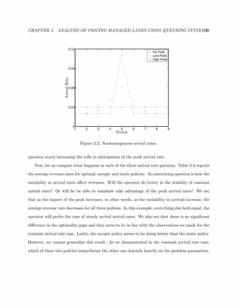
CHAPTER 2. ANALYSIS OF PRICING MANAGED LANES USING QUEUEING SYSTEMS48
1 2 3 4 5 6 7 8 90
0.03
0.06
0.09
0.12
Period
ArrivalRate
No PeakLow PeakHigh Peak
Figure 2.2: Nonhomogenous arrival rates.
operator starts increasing the tolls in anticipation of the peak arrival rate.
Now, let us compare what happens in each of the three arrival rate patterns. Table 2.3 reports
the average revenue rates for optimal, myopic and static policies. An interesting question is how the
variability in arrival rates affect revenues. Will the operator do better in the stability of constant
arrival rates? Or will he be able to somehow take advantage of the peak arrival rates? We see
that as the impact of the peak increases, in other words, as the variability in arrivals increase, the
average revenue rate decreases for all three policies. In this example, everything else held equal, the
operator will prefer the case of steady arrival arrival rates. We also see that there is no significant
difference in the optimality gaps and they seem to be in line with the observations we made for the
constant arrival rate case. Lastly, the myopic policy seems to be doing better than the static policy.
However, we cannot generalize this result. As we demonstrated in the constant arrival rate case,
which of these two policies outperforms the other one depends heavily on the problem parameters.

CHAPTER 2. ANALYSIS OF PRICING MANAGED LANES USING QUEUEING SYSTEMS49
1 3 5 7 90
0.02
0.04
0.06
Period
ArrivalRate
1 3 5 7 90.994
0.996
0.998
1
1.002
1.004
1.006
NormalizedToll
Arrival RateNormalized Toll
(a) Low peak case.
1 3 5 7 90
0.02
0.04
0.06
0.08
0.1
0.12
Period
ArrivalRate
1 3 5 7 90.994
0.996
0.998
1
1.002
1.004
1.006
NormalizedToll
Arrival RateNormalized Toll
(b) High peak case.
Figure 2.3: Normalized optimal tolls and arrival rates.
1 3 5 7 90
0.02
0.04
0.06
Period
ArrivalRate
1 3 5 7 9292
293
294
295
296
297
298
Static
Toll
Arrival RateStatic Toll
(a) Low peak case.
1 3 5 7 90
0.02
0.04
0.06
0.08
0.1
0.12
Period
ArrivalRate
1 3 5 7 9292
293
294
295
296
297
298
Static
Toll
Arrival RateStatic Toll
(b) High peak case.
Figure 2.4: Static tolls and arrival rates.
2.4 Conclusion
In this chapter we analyzed the problem of setting revenue maximizing tolls for managed lanes.
Our model was based on M/M/1 queueing models and allowed us to analyze the first order effects
of congestion. We also introduced a variant of the stochastic model that takes into account the
non-homogeneity of the traffic flows.
We found that dynamic pricing can provide significant revenue improvements over both static
and myopic policies. We showed that the optimal policy has a very simple form. It is monotonic
with respect to the number of cars in the system. Furthermore, we demonstrated that the myopic

CHAPTER 2. ANALYSIS OF PRICING MANAGED LANES USING QUEUEING SYSTEMS50
policy always underprices compared to the dynamic policy. We observed that the relative difference
between myopic and optimal tolls decreases as the unmanaged lanes are relatively more congested.
For the time-varying arrival rate case we observed that the toll operator should increase the tolls
before the peak arrival period. In the next chapter we will see that this aspect of the optimal tolling
strategy turns out to be crucial.
We believe that the modeling approach we employ in the non-homogeneous arrival rate case
can find applications in other areas where repetitive cyclic demand is observed, e.g. as call center
staffing. An interesting open question is how the results in this chapter would change if the focus
was on social welfare maximizing policies.
Case Optimal Myopic Static Myopic Pol. Gap Static Pol. Gap
No Peak 9.43 8.11 7.34 14.03% 22.16%Low Peak 9.39 8.08 7.31 13.97% 22.23%High Peak 9.26 7.98 7.18 13.77% 22.44%
Table 2.3: Average revenue rates for different arrival patterns.

CHAPTER 3. SIMULATION BASED OPTIMIZATION FOR PRICING MANAGED LANES51
Chapter 3
Simulation Based Optimization for
Pricing Managed Lanes
In this chapter we continue analyzing the pricing of managed lanes. Unlike the previous chapter,
we take a more practical point of view of the problem. Through the use of a traffic simulator,
we demonstrate how revenue maximizing tolls can be computed in practice. We also conduct an
extensive numerical study to analyze the impact of such policies.
3.1 Traffic Simulation
We borrow our simulation methodology from the dynamic traffic assignment (DTA) literature that
primarily deals with the problem of computing the user equilibrium and system optimal traffic flows
on a transportation network. The solution approaches to these problems can be classified in two
categories: analytical and simulation Peeta and Ziliaskopoulos (2001). Analytical approaches typ-
ically employ tools such as mathematical programming, optimal control and variational inequality
to model traffic systems. Due to the ill-behaved nature of DTA problems, they are unsuitable for
applications such as ours where real-time decisions influence drivers’ behavior (Burghout, 2005).
Simulations can be categorized as macroscopic, microscopic and mesoscopic. In macroscopic
simulations, aggregate traffic flows are calculated and individual vehicles are not modeled. Since

CHAPTER 3. SIMULATION BASED OPTIMIZATION FOR PRICING MANAGED LANES52
they do not model individual behavior, we cannot incorporate how drivers react to congestion and
toll changes when they are making their routing decisions (Burghout, 2005). Two well known
macroscopic simulation models are the LWR model that was devised by Lighthill and Whitham
(1955) and Richards (1956), and the cell transmission model (CTM) that was introduced by Da-
ganzo (1994).
Unlike macroscopic simulations, mesoscopic and microscopic simulations capture a greater level
of detail by keeping track of individual vehicles with the latter being more detailed. Microscopic
simulations model traffic dynamics in a detailed manner by building upon car following and lane
changing models that are prevalent in the literature. This enables the microscopic approach to
model the interactions between drivers themselves and how they change their behavior with chang-
ing road conditions. MITSIM, VISSIM and PARAMICS are some of the most well known micro-
scopic simulation models (Olstam and Tapani, 2004).
However, the level of detail that microscopic simulations can capture comes at an additional
cost. Compared to the other two approaches, there are many more parameters in this model that
require calibration and the computational time required to run such a model is considerably much
longer. Therefore, we will be employing the mesoscopic simulation approach in this study. In
mesoscopic simulations the road is typically divided into several links and at each time step the
vehicles are moved from one link to another by making use of speed, flow, and density relationships.
The two most prominent mesoscopic simulation models are the DYNASMART (Jayakrishnan et
al., 1994) and the DynaMIT (Ben-Akiva et al., 2002) upon which our simulation model is based.
In our context, these two models are almost identical with the exception of a few details.
3.1.1 Model Description
In our traffic module, the highway is divided into various segments with equal length L. The number
of lanes in each segment is denoted by w and the average space that a car occupies (including its
headway at jam density) will be denoted by `. As a result, the physical capacity of each segment
is w × L/`.
The segments will be split into two parts: moving and queueing. Cars that are queued up to
CHAPTER 3. SIMULATION BASED OPTIMIZATION FOR PRICING MANAGED LANES53
join the next segment will be in the queueing part and the remainder of the cars in the segment
will be in the moving part. The lengths of both parts are dynamic and depend on the number of
cars in the queueing part. Given that there are nq cars queued, the length of the queueing part is
nq`/w. Accordingly, the length of the moving part is L− nq`/w.
At each time step in our simulation, the vehicles in the moving part will traverse the segment
according to the following two-regime speed-density relationship
v(k) =
vmax + β1k, if k ≤ kbp,
vmin + β2(1− (k/kj)α1)α2 , if k > kbp,
(3.1)
where k is the density of the moving part of the segment at the beginning of the time step, vmax
is the free-flow speed, vmin is the minimum speed, kj is the jam density, and α1, α2, β1 and β2
are user-specified parameters. All speeds are in mph and densities are in vehicles/mile/lane unless
otherwise noted. After a car has traversed a segment it has two options. If there is space in the
next segment, it will pass on to that segment directly and travel on that segment for the remainder
of the time step. Otherwise, it will join a queue at the end of the segment.
In each time step the movement of cars is calculated in three stages. In the first stage, cars in
the moving segment move according to the speed-density relationships in (3.1), and the ones that
reach the end of the segment move into a queue to await transition into the next segment. We
update the position of each car starting from the one that is closest to the highway’s end and move
towards the beginning of the highway. In the next step, cars move from the queues at the end of
each segment to the next segment. Cars are allowed to pass on to the next segment until it reaches
jam density. We allow partial cars to pass on to the next segment. The last step involves moving
the cars that just changed segments. If a car waited in the queue for at least one iteration, then it
is moved according to the prevailing moving part speed of its previous segment. Otherwise, that is
if the car joined the queue in that iteration, it completes its movement by traveling the amount it
was not allowed to complete before joining the queue.
Once the vehicles are moved, we calculate the expected travel times for each segment. The
CHAPTER 3. SIMULATION BASED OPTIMIZATION FOR PRICING MANAGED LANES54
expected travel time for each segment consists of the time it takes for a vehicle to traverse the
moving part of a segment (Tm), and the waiting time in the queue (Tw). Let qw denote the number
of cars waiting in the queueing part of a segment, then the moving time is,
Tm =L− qw × `× w
v(k),
and the waiting time is,
Tw = qw/d,
where d is the moving average of the discharge rates observed in the previous periods. Those times
are calculated for each segment and are turn used to calculate the expected travel time for both
parts of the highway. The travel times are fed into the consumer choice model to calculate the
demand for each part of the highway at the next time step.
Our traffic flow model is structurally identical to DYNASMART. It is also similar to DynaMIT,
although we use a slightly different approach to calculate moving times and waiting times. These
models have been used in many studies and have been extensively validated (Han et al., 2006;
Roelofsen, 2012; Ben-Akiva et al., 2010).
3.1.2 Traffic Simulation Calibration
In our simulation, the speed in each segment is determined by the density in that segment according
to equation (3.1). Figure 3.1 shows a scatterplot of the speed and density for the unmanaged lanes
in the SR-91, for weekdays during the first four weeks of July 2011. We chose this period because
there was no rain. The data is obtained through PeMS for VDS 1208147 with an aggregation
level of 5 minutes. We deleted approximately 17% of the datapoints as outliers resulting from lane
closures and accidents, resulting in 5,760 observations.
The black line in Figure 2 is the speed-density relationship that we fit to this data. We set
the jam density to 100 vehicles/mile/lane since there were only three observations with densities
greater than 100. We eliminated those three observations from our dataset. We set the minimum
speed vmin to 15 mph in accordance with the average speed observed when density is around 100

CHAPTER 3. SIMULATION BASED OPTIMIZATION FOR PRICING MANAGED LANES55
0 20 40 60 80 1000
10
20
30
40
50
60
70
80
Density (vechiles/mile/lane)
Speed(m
ph)
Figure 3.1: Speed-density relationship for SR-91.
vehicles/mile/lane. We set the simulation time-step to a minute. We found that the moving average
of the last five periods gave a fairly accurate representation of the discharge rate from each segment
when it is congested.
We set the breakpoint density to 25 vcl/m/ln because it minimizes the sum of squared residuals
from both models. We used OLS regression to estimated the parameters for the first (linear)
regime and NLS regression to estimate the parameters in the second (nonlinear) regime. After the
estimation procedure we readjusted β2 to avoid discontinuity at the breakpoint density. Table 3.1
gives the parameters we used in the simulation that were obtained through the abovementioned
estimation procedure.
Since the current SR-91 policy sets tolls to encourage free-flow conditions in the managed lanes,
there is no data for more congested conditions in the managed lanes. For this reason, we use
the same speed-density relationship given by Figure 3.1 for both parts of the highway. Since the
Speed (mph) Density (vcl/m/ln) Slope Shape
vmin 15.00 kbp 25 β1 -0.14 α1 2.22vmax 66.80 kj 100 β2 69.33 α2 7.69
Table 3.1: Parameters for the simulation model.
CHAPTER 3. SIMULATION BASED OPTIMIZATION FOR PRICING MANAGED LANES56
managed lanes run parallel to the unmanaged lanes, this is a reasonable assumption.
Similar to SR-91, the number of managed lanes is set to two. The number of unmanaged
lanes on the SR-91 differs between four and five. In addition, different sections of the highway
have different speed-density relationships. For the purposes of this study, we will assume that the
highway we are analyzing is 10 miles long and consists uniformly of five unmanaged lanes with the
speed density relationship given in Table 3.1. Since we are not accounting for the full geometric
structure of SR-91, the travel times obtained by this simulation do not accurately represent the
travel times observed on the SR-91.
3.2 Demand Generation
We generate traffic arriving to the system in two steps. In the first step we generate hourly demands,
and in the second step we distribute the hourly traffic into five-minute intervals.
To calibrate the hourly demand generator we used the eastbound hourly flow information for the
SR91 from January 2009 to August 2011. We combine the volume information from the managed
and unmanaged lanes to calculate the total volume of traffic using the highway. Traffic data for
managed lanes comes from VDS 1208156 and for unmanaged lanes we use the data from VDS
1208147. Figure 3.2 depicts the average hourly traffic volumes for each day of the week for Monday
through Friday. From the figure we can see that the arrival pattern is very similar for all days.
Thus, we will use the same hourly demands for each day of the week.
Starting from midnight, we generate hourly traffic loads according to
Yt = βt + α1tYt−1 + α2
tYt−2 + α3tYt−3 + εt, (3.2)
where Yt is the traffic volume for hour t; βt, α1t , α
2t and α3
t are coefficients and εt is a normally
distributed error term. We estimated the parameters of (3.2) using OLS regression. To start
generating hourly loads from midnight and onwards, we need starting values for the hours 21, 22
and 23. For simplicity, we sampled the demand for these three hours from normal distributions
whose means, standard deviations and pairwise correlations match their real-life values. These
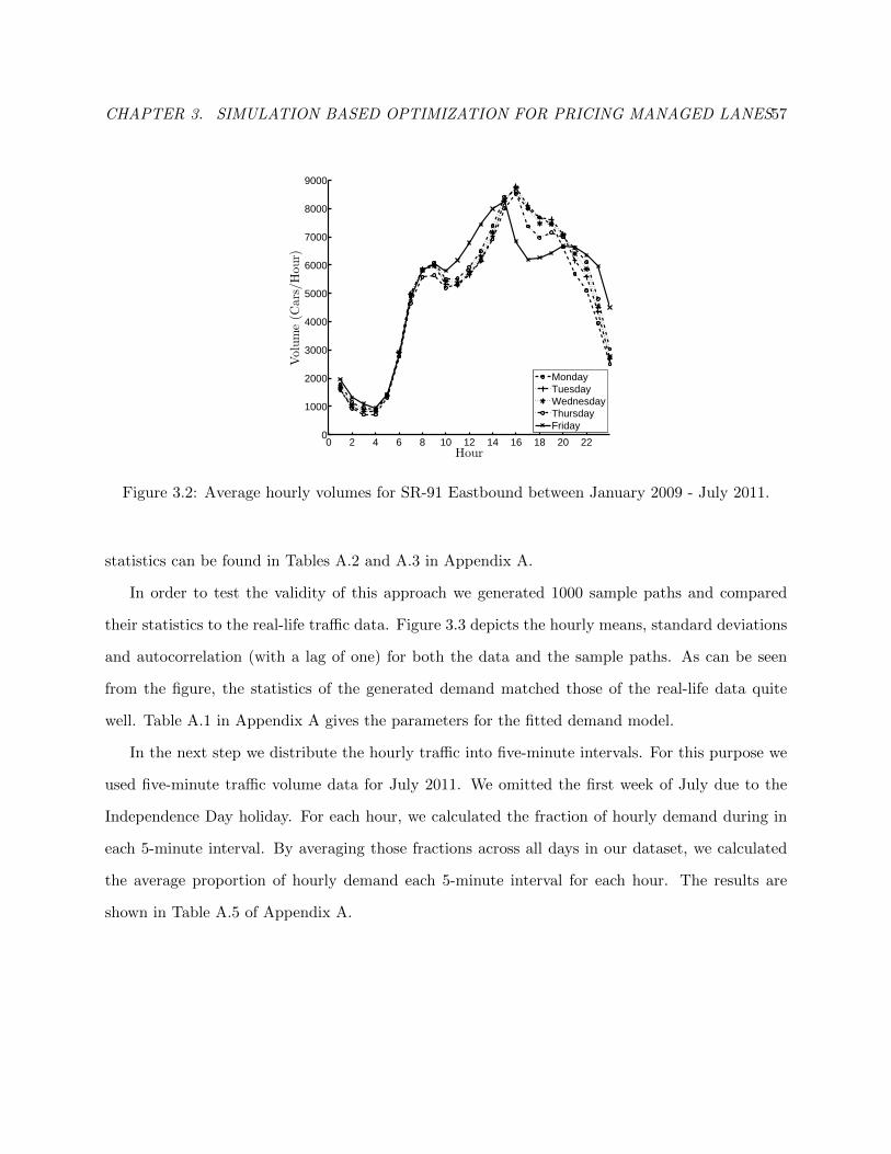
CHAPTER 3. SIMULATION BASED OPTIMIZATION FOR PRICING MANAGED LANES57
0 2 4 6 8 10 12 14 16 18 20 220
1000
2000
3000
4000
5000
6000
7000
8000
9000
Hour
Volume(C
ars/Hour)
MondayTuesdayWednesdayThursdayFriday
Figure 3.2: Average hourly volumes for SR-91 Eastbound between January 2009 - July 2011.
statistics can be found in Tables A.2 and A.3 in Appendix A.
In order to test the validity of this approach we generated 1000 sample paths and compared
their statistics to the real-life traffic data. Figure 3.3 depicts the hourly means, standard deviations
and autocorrelation (with a lag of one) for both the data and the sample paths. As can be seen
from the figure, the statistics of the generated demand matched those of the real-life data quite
well. Table A.1 in Appendix A gives the parameters for the fitted demand model.
In the next step we distribute the hourly traffic into five-minute intervals. For this purpose we
used five-minute traffic volume data for July 2011. We omitted the first week of July due to the
Independence Day holiday. For each hour, we calculated the fraction of hourly demand during in
each 5-minute interval. By averaging those fractions across all days in our dataset, we calculated
the average proportion of hourly demand each 5-minute interval for each hour. The results are
shown in Table A.5 of Appendix A.
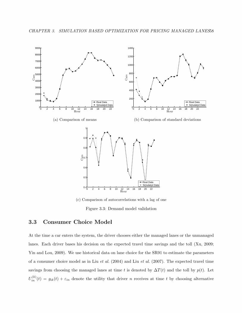
CHAPTER 3. SIMULATION BASED OPTIMIZATION FOR PRICING MANAGED LANES58
0 2 4 6 8 10 12 14 16 18 20 220
1000
2000
3000
4000
5000
6000
7000
8000
9000
Hour
Cars
Real DataSimulated Data
(a) Comparison of means
0 2 4 6 8 10 12 14 16 18 20 220
200
400
600
800
1000
1200
1400
Hour
Cars
Real DataSimulated Data
(b) Comparison of standard deviations
0 2 4 6 8 10 12 14 16 18 20 220.4
0.5
0.6
0.7
0.8
0.9
1
Hour
Cars
Real DataSimulated Data
(c) Comparison of autocorrelations with a lag of one
Figure 3.3: Demand model validation
3.3 Consumer Choice Model
At the time a car enters the system, the driver chooses either the managed lanes or the unmanaged
lanes. Each driver bases his decision on the expected travel time savings and the toll (Xu, 2009;
Yin and Lou, 2009). We use historical data on lane choice for the SR91 to estimate the parameters
of a consumer choice model as in Liu et al. (2004) and Liu et al. (2007). The expected travel time
savings from choosing the managed lanes at time t is denoted by ∆T (t) and the toll by p(t). Let
U(k)in (t) = gik(t) + εin denote the utility that driver n receives at time t by choosing alternative
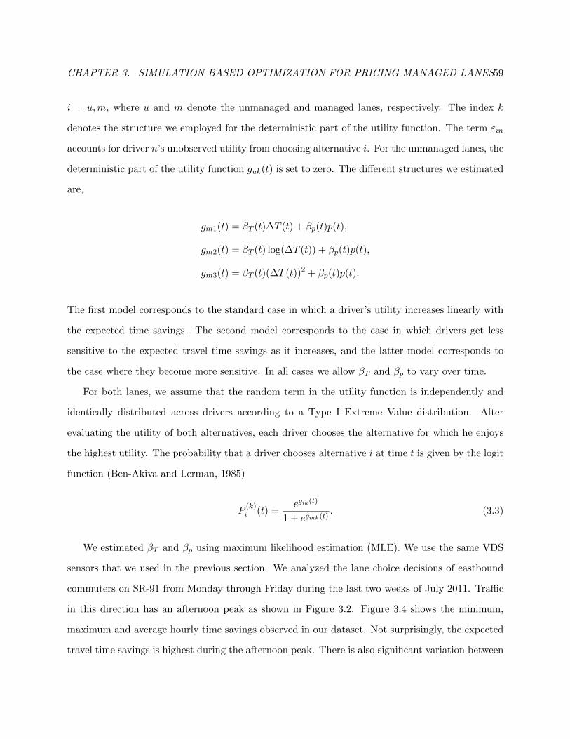
CHAPTER 3. SIMULATION BASED OPTIMIZATION FOR PRICING MANAGED LANES59
i = u,m, where u and m denote the unmanaged and managed lanes, respectively. The index k
denotes the structure we employed for the deterministic part of the utility function. The term εin
accounts for driver n’s unobserved utility from choosing alternative i. For the unmanaged lanes, the
deterministic part of the utility function guk(t) is set to zero. The different structures we estimated
are,
gm1(t) = βT (t)∆T (t) + βp(t)p(t),
gm2(t) = βT (t) log(∆T (t)) + βp(t)p(t),
gm3(t) = βT (t)(∆T (t))2 + βp(t)p(t).
The first model corresponds to the standard case in which a driver’s utility increases linearly with
the expected time savings. The second model corresponds to the case in which drivers get less
sensitive to the expected travel time savings as it increases, and the latter model corresponds to
the case where they become more sensitive. In all cases we allow βT and βp to vary over time.
For both lanes, we assume that the random term in the utility function is independently and
identically distributed across drivers according to a Type I Extreme Value distribution. After
evaluating the utility of both alternatives, each driver chooses the alternative for which he enjoys
the highest utility. The probability that a driver chooses alternative i at time t is given by the logit
function (Ben-Akiva and Lerman, 1985)
P(k)i (t) =
egik(t)
1 + egmk(t). (3.3)
We estimated βT and βp using maximum likelihood estimation (MLE). We use the same VDS
sensors that we used in the previous section. We analyzed the lane choice decisions of eastbound
commuters on SR-91 from Monday through Friday during the last two weeks of July 2011. Traffic
in this direction has an afternoon peak as shown in Figure 3.2. Figure 3.4 shows the minimum,
maximum and average hourly time savings observed in our dataset. Not surprisingly, the expected
travel time savings is highest during the afternoon peak. There is also significant variation between
CHAPTER 3. SIMULATION BASED OPTIMIZATION FOR PRICING MANAGED LANES60
1 3 5 7 9 11 13 15 17 19 21 230
5
10
15
20
25
30
35
40
45
Hour
AverageTim
eSavings(m
in)
AverageMinimumMaximum
Figure 3.4: Average hourly time savings.
the time savings observed throughout this two week period.
From Figure 3.5 we can see that managed lanes traffic peaks in the afternoon when both
the traffic load and the time savings are highest. During the off-peak hours, the managed lanes
command a very low share of the traffic passing through this segment of the highway.
Currently, in SR-91 tolls are set ahead of time and vary hourly. Figure 3.6 shows how the tolls
varied from Monday through Friday in the July-December 2011 period. The variation in tolls is
quite dramatic: during the off-peak hours the toll goes as low as $1.30, and during the peak hours
it is as high as $9.75. The aim of the SR-91 operator is to maintain free-flow conditions on the
managed lanes. As a result, the structure of the tolls mirrors the expected travel time savings quite
closely. The operator updates the tolls every few months to adjust for changing traffic patterns.
The SR-91’s policy leads to high correlation between the tolls and time savings. Similar to
Lam and Small (2001), to come up with estimates for βT and βp we exploit the variation in time
savings during the peak hours when the tolls do not change very much. Figure 3.7 plots the average
ratio of expected time savings to tolls in five minute intervals. There is significant variation in that
ratio during both peak and early morning hours. For our analysis we choose the afternoon peak
hours, specifically between the hours of 2pm and 8pm, since the traffic volume is significantly higher
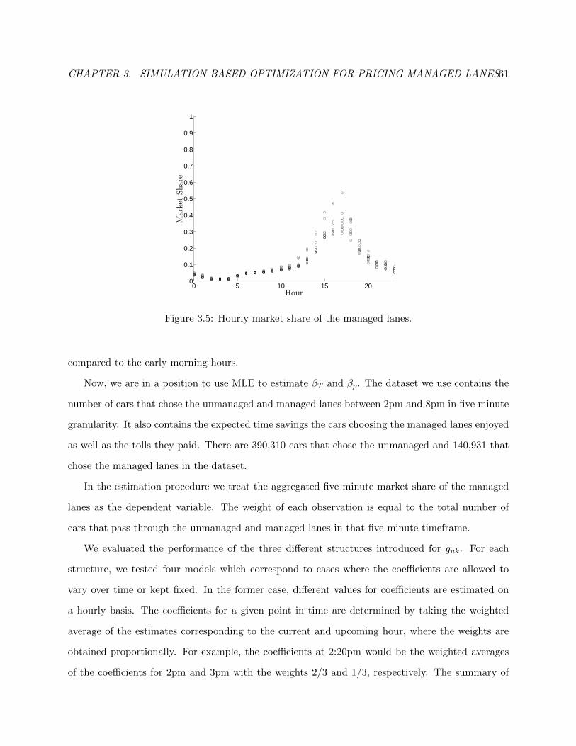
CHAPTER 3. SIMULATION BASED OPTIMIZATION FOR PRICING MANAGED LANES61
0 5 10 15 200
0.1
0.2
0.3
0.4
0.5
0.6
0.7
0.8
0.9
1
Hour
MarketShare
Figure 3.5: Hourly market share of the managed lanes.
compared to the early morning hours.
Now, we are in a position to use MLE to estimate βT and βp. The dataset we use contains the
number of cars that chose the unmanaged and managed lanes between 2pm and 8pm in five minute
granularity. It also contains the expected time savings the cars choosing the managed lanes enjoyed
as well as the tolls they paid. There are 390,310 cars that chose the unmanaged and 140,931 that
chose the managed lanes in the dataset.
In the estimation procedure we treat the aggregated five minute market share of the managed
lanes as the dependent variable. The weight of each observation is equal to the total number of
cars that pass through the unmanaged and managed lanes in that five minute timeframe.
We evaluated the performance of the three different structures introduced for guk. For each
structure, we tested four models which correspond to cases where the coefficients are allowed to
vary over time or kept fixed. In the former case, different values for coefficients are estimated on
a hourly basis. The coefficients for a given point in time are determined by taking the weighted
average of the estimates corresponding to the current and upcoming hour, where the weights are
obtained proportionally. For example, the coefficients at 2:20pm would be the weighted averages
of the coefficients for 2pm and 3pm with the weights 2/3 and 1/3, respectively. The summary of
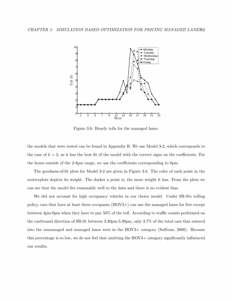
CHAPTER 3. SIMULATION BASED OPTIMIZATION FOR PRICING MANAGED LANES62
1 3 5 7 9 11 13 15 17 19 21 230
1
2
3
4
5
6
7
8
9
10
Hour
Toll($)
MondayTuesdayWednesdayThursdayFriday
Figure 3.6: Hourly tolls for the managed lanes.
the models that were tested can be found in Appendix B. We use Model 3-2, which corresponds to
the case of k = 3, as it has the best fit of the model with the correct signs on the coefficients. For
the hours outside of the 2-8pm range, we use the coefficients corresponding to 8pm.
The goodness-of-fit plots for Model 3-2 are given in Figure 3.8. The color of each point in the
scatterplots depicts its weight. The darker a point is, the more weight it has. From the plots we
can see that the model fits reasonably well to the data and there is no evident bias.
We did not account for high occupancy vehicles in our choice model. Under SR-91s tolling
policy, cars that have at least three occupants (HOV3+) can use the managed lanes for free except
between 4pm-6pm when they have to pay 50% of the toll. According to traffic counts performed on
the eastbound direction of SR-91 between 3.30pm-5.30pm, only 3.7% of the total cars that entered
into the unmanaged and managed lanes were in the HOV3+ category (Sullivan, 2000). Because
this percentage is so low, we do not feel that omitting the HOV3+ category significantly influenced
our results.

CHAPTER 3. SIMULATION BASED OPTIMIZATION FOR PRICING MANAGED LANES63
0 2 4 6 8 10 12 14 16 18 20 22 240.5
1
1.5
2
2.5
3
3.5
Hour
Tim
eSavingsto
TollsRatio
Figure 3.7: The average ratio of time savings to tolls.
3.4 Problem Formulation
3.4.1 Policy Description
Our goal is to compare policies for the managed lanes in terms of expected revenue generated.
We consider both adaptive and non-adaptive policies. Adaptive policies adjust tolls dynamically
depending on real-time traffic conditions, whereas non-adaptive ones keep tolls fixed regardless of
the system’s state.
We use a discrete time approach in which we divide the planning horizon into T intervals, and t
denotes the interval index. The number of cars that arrive in an interval is random, and is denoted
by the random variable D(t). We assume that the toll stays constant over each interval. This is
non-restrictive because all dynamic tolling schemes implemented to date enforce a minimum period
between toll changes – for example, five minutes in the case of the LBJ Project. For the remainder
of this section, the subscripts u and m denote unmanaged and managed lanes, respectively. The
number of cars in the lanes and their locations are denoted by xi(t) for i = u,m.
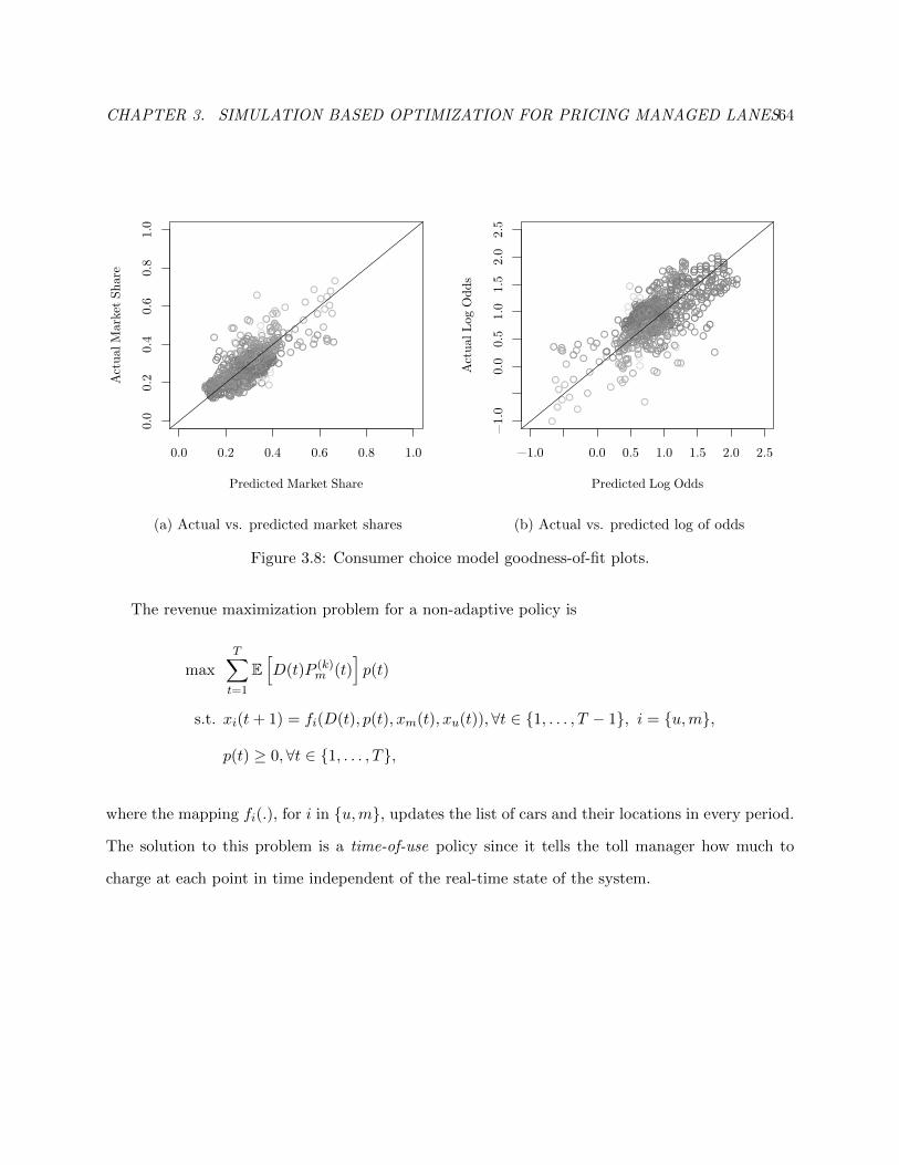
CHAPTER 3. SIMULATION BASED OPTIMIZATION FOR PRICING MANAGED LANES64
0.0 0.2 0.4 0.6 0.8 1.0
0.0
0.2
0.4
0.6
0.8
1.0
Predicted Market Share
Actu
al M
arket
Share
(a) Actual vs. predicted market shares
−1.0 0.0 0.5 1.0 1.5 2.0 2.5
−1.0
0.0
0.5
1.0
1.5
2.0
2.5
Predicted Log Odds
Act
ual L
og O
dds
(b) Actual vs. predicted log of odds
Figure 3.8: Consumer choice model goodness-of-fit plots.
The revenue maximization problem for a non-adaptive policy is
max
T∑t=1
E[D(t)P (k)
m (t)]p(t)
s.t. xi(t+ 1) = fi(D(t), p(t), xm(t), xu(t)),∀t ∈ 1, . . . , T − 1, i = u,m,
p(t) ≥ 0,∀t ∈ 1, . . . , T,
where the mapping fi(.), for i in u,m, updates the list of cars and their locations in every period.
The solution to this problem is a time-of-use policy since it tells the toll manager how much to
charge at each point in time independent of the real-time state of the system.
CHAPTER 3. SIMULATION BASED OPTIMIZATION FOR PRICING MANAGED LANES65
The discrete-time counterpart of the adaptive policy is
maxT∑t=1
E[D(t)P (k)
m (t)]p(t, xu(t), xm(t))
s.t. xi(t+ 1) = fi(D(t), p(t, xu(t), xm(t)), xm(t), xu(t)), ∀t ∈ 1, . . . , T − 1, i = u,m,
p(xu(t), xm(t)) ≥ 0, ∀t ∈ [0, T ].
Compared to the previous model, the toll is now dependent on the state of the system at each point
in time as well as the time. The optimal adaptive policy is quite hard to compute due to the curse
of dimensionality. We consider two simple heuristics.
The myopic tolling policy maximizes the revenue rate from the system according to the current
travel time difference:
p(t) = argmaxp≥0P(k)m (t)p.
The major shortcoming of the myopic policy is its inability to take into account the future congestion
effects due to the lane choice of arriving traffic. This also contributes to the simplicity of this policy
since no calibration is necessary to implement it. Every time the toll is updated, the revenue rate
maximizing toll can be computed numerically. We employ Brent’s method which is a popular robust
derivative-free approach for this purpose (Brent, 2002).
We also consider a more complex adaptive policy. This policy takes a set of base time-of-use
tolls p(t)Tt=1 and travel time savings ∆T (t)Tt=1 as inputs. Every time the toll is updated, it
compares the current travel time savings to the base values. If the system is more congested than
expected, the policy increases the toll relative to the base toll. If there is less congestion than
expected, the policy decreases the toll. The form of this policy is given by
p(t,∆T (t)) = p(t) + α+(t)(∆T (t)−∆T (t))+ − α−(t)(∆T (t)−∆T (t))+, (3.4)
where α+(t) and α−(t) are positive scalars. Since the tolling adjustments are based on linear travel
time differences, we call this policy as the linear travel time difference (LinTD) policy.

CHAPTER 3. SIMULATION BASED OPTIMIZATION FOR PRICING MANAGED LANES66
3.4.2 Policy Calibration
In order to calibrate these two policies we used a combination of nonlinear optimization heuristics
and stochastic approximation.
Our calibration strategy for both policies can be summarized as follows. First, we employed non-
linear optimization heuristics such as the Nelder-Mead and Brent’s method to find initial starting
points. Later, we fed these starting points into the stochastic approximation optimization routine.
Stochastic optimization problems are generally solved by iterative algorithms that start from
some trial solution and update the trial solution using the stochastic gradient of the objective
function. For maximization problems, this procedure is of the following iterative form
xk+1 = xk + akgk(xk),
where k is the iteration index, xk ∈ Rn denotes the current solution, ak ∈ Rn+ is the updating
step size that typically decreases in k, and gk(.) is the stochastic gradient estimate. If there are
any constraints on the decision variables, the updated values are projected onto the set of feasible
values to ensure that the constraints are satisfied.
Since no direct measurements of the gradient are available in our case, we employ the finite
differences stochastic approximation (FDSA) method that estimates the gradient by calculating the
difference quotient one-by-one for each decision variable using the Monte Carlo method. Kiefer and
Wolfowitz (1952) introduced this method for univariate optimization problems and Blum (1954)
extended it to the multivariate case. Let Ω denote the set of possible realizations of a random
process, and y(x, ω) be a function whose value depends on some variable x ∈ Rn and the realization
of the random outcome ω ∈ Ω. Using the FDSA method the gradient estimate of y(.) for each
iteration is obtained by
(gk(xk))i =m∑j=1
y(xk + eick, ωkj)− y(xk − eick, ωki)2ck
, ∀i = 1, . . . , n,
where cki is a small positive scalar that decreases in k, and ei ∈ Rn is the unit vector in direction i.
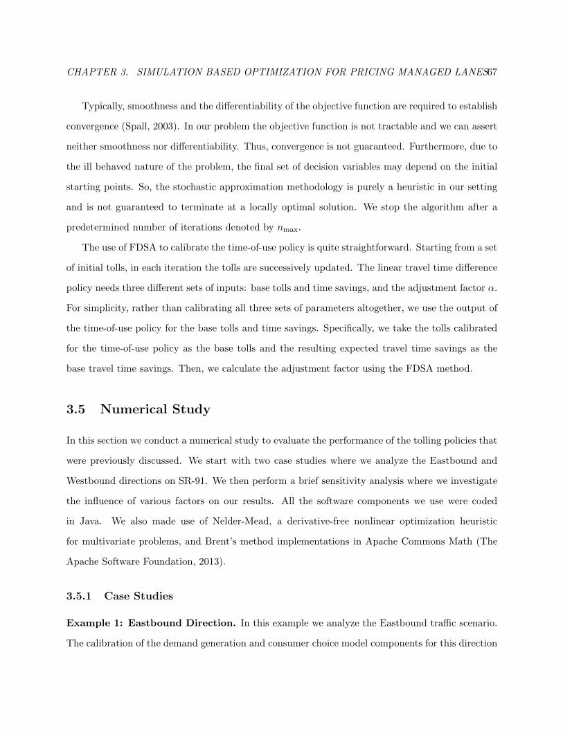
CHAPTER 3. SIMULATION BASED OPTIMIZATION FOR PRICING MANAGED LANES67
Typically, smoothness and the differentiability of the objective function are required to establish
convergence (Spall, 2003). In our problem the objective function is not tractable and we can assert
neither smoothness nor differentiability. Thus, convergence is not guaranteed. Furthermore, due to
the ill behaved nature of the problem, the final set of decision variables may depend on the initial
starting points. So, the stochastic approximation methodology is purely a heuristic in our setting
and is not guaranteed to terminate at a locally optimal solution. We stop the algorithm after a
predetermined number of iterations denoted by nmax.
The use of FDSA to calibrate the time-of-use policy is quite straightforward. Starting from a set
of initial tolls, in each iteration the tolls are successively updated. The linear travel time difference
policy needs three different sets of inputs: base tolls and time savings, and the adjustment factor α.
For simplicity, rather than calibrating all three sets of parameters altogether, we use the output of
the time-of-use policy for the base tolls and time savings. Specifically, we take the tolls calibrated
for the time-of-use policy as the base tolls and the resulting expected travel time savings as the
base travel time savings. Then, we calculate the adjustment factor using the FDSA method.
3.5 Numerical Study
In this section we conduct a numerical study to evaluate the performance of the tolling policies that
were previously discussed. We start with two case studies where we analyze the Eastbound and
Westbound directions on SR-91. We then perform a brief sensitivity analysis where we investigate
the influence of various factors on our results. All the software components we use were coded
in Java. We also made use of Nelder-Mead, a derivative-free nonlinear optimization heuristic
for multivariate problems, and Brent’s method implementations in Apache Commons Math (The
Apache Software Foundation, 2013).
3.5.1 Case Studies
Example 1: Eastbound Direction. In this example we analyze the Eastbound traffic scenario.
The calibration of the demand generation and consumer choice model components for this direction
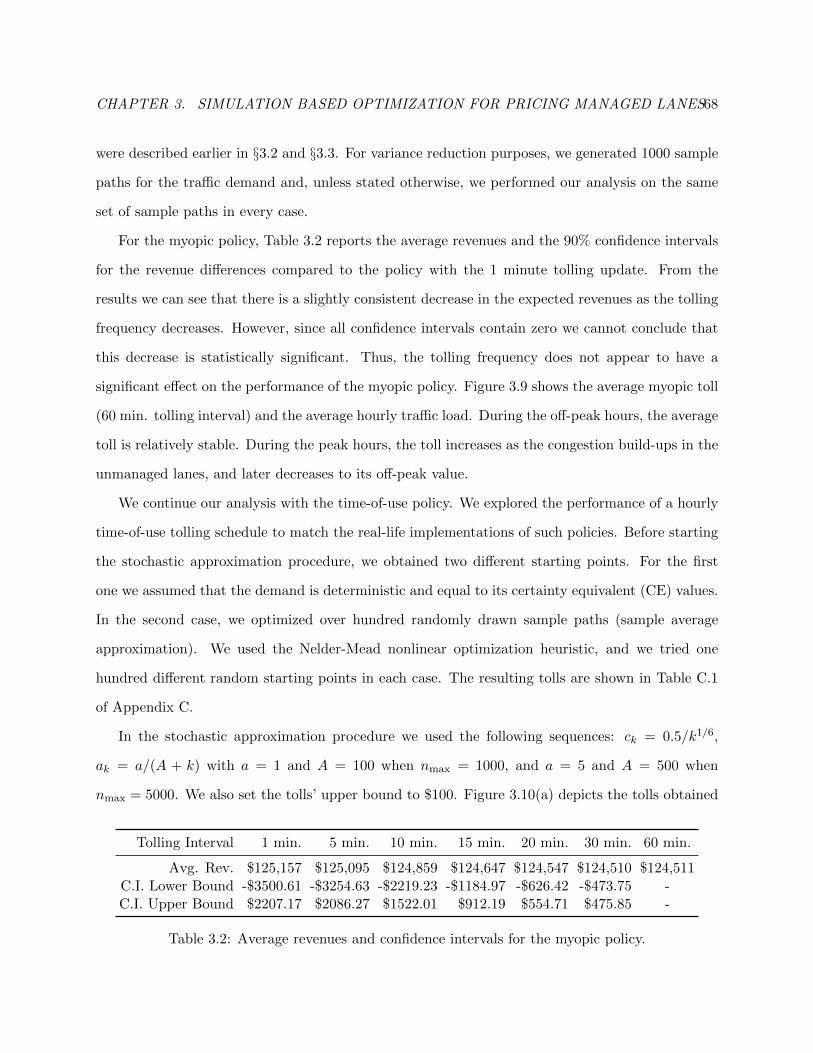
CHAPTER 3. SIMULATION BASED OPTIMIZATION FOR PRICING MANAGED LANES68
were described earlier in §3.2 and §3.3. For variance reduction purposes, we generated 1000 sample
paths for the traffic demand and, unless stated otherwise, we performed our analysis on the same
set of sample paths in every case.
For the myopic policy, Table 3.2 reports the average revenues and the 90% confidence intervals
for the revenue differences compared to the policy with the 1 minute tolling update. From the
results we can see that there is a slightly consistent decrease in the expected revenues as the tolling
frequency decreases. However, since all confidence intervals contain zero we cannot conclude that
this decrease is statistically significant. Thus, the tolling frequency does not appear to have a
significant effect on the performance of the myopic policy. Figure 3.9 shows the average myopic toll
(60 min. tolling interval) and the average hourly traffic load. During the off-peak hours, the average
toll is relatively stable. During the peak hours, the toll increases as the congestion build-ups in the
unmanaged lanes, and later decreases to its off-peak value.
We continue our analysis with the time-of-use policy. We explored the performance of a hourly
time-of-use tolling schedule to match the real-life implementations of such policies. Before starting
the stochastic approximation procedure, we obtained two different starting points. For the first
one we assumed that the demand is deterministic and equal to its certainty equivalent (CE) values.
In the second case, we optimized over hundred randomly drawn sample paths (sample average
approximation). We used the Nelder-Mead nonlinear optimization heuristic, and we tried one
hundred different random starting points in each case. The resulting tolls are shown in Table C.1
of Appendix C.
In the stochastic approximation procedure we used the following sequences: ck = 0.5/k1/6,
ak = a/(A + k) with a = 1 and A = 100 when nmax = 1000, and a = 5 and A = 500 when
nmax = 5000. We also set the tolls’ upper bound to $100. Figure 3.10(a) depicts the tolls obtained
Tolling Interval 1 min. 5 min. 10 min. 15 min. 20 min. 30 min. 60 min.
Avg. Rev. $125,157 $125,095 $124,859 $124,647 $124,547 $124,510 $124,511C.I. Lower Bound -$3500.61 -$3254.63 -$2219.23 -$1184.97 -$626.42 -$473.75 -C.I. Upper Bound $2207.17 $2086.27 $1522.01 $912.19 $554.71 $475.85 -
Table 3.2: Average revenues and confidence intervals for the myopic policy.
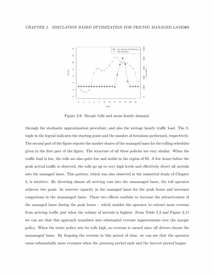
CHAPTER 3. SIMULATION BASED OPTIMIZATION FOR PRICING MANAGED LANES69
Hour
Tol
l ($
)
0 2 4 6 8 10 12 14 16 18 20 22
02
46
810
1214
020
0040
0060
0080
0010
000
Car
s/H
our
Avg. Myopic Toll (60 min.)Avg. Demand
Figure 3.9: Myopic tolls and mean hourly demand.
through the stochastic approximation procedure, and also the average hourly traffic load. The 2-
tuple in the legend indicates the starting point and the number of iterations performed, respectively.
The second part of the figure reports the market shares of the managed lanes for the tolling schedules
given in the first part of the figure. The structure of all three policies are very similar. When the
traffic load is low, the tolls are also quite low and stable in the region of $3. A few hours before the
peak arrival traffic is observed, the tolls go up to very high levels and effectively divert all arrivals
into the managed lanes. This pattern, which was also observed in the numerical study of Chapter
2, is intuitive. By diverting almost all arriving cars into the unmanaged lanes, the toll operator
achieves two goals: he reserves capacity in the managed lanes for the peak hours and increases
congestions in the unmanaged lanes. These two effects combine to increase the attractiveness of
the managed lanes during the peak hours – which enables the operator to extract more revenue
from arriving traffic just when the volume of arrivals is highest. From Table 3.3 and Figure 3.11
we can see that this approach translates into substantial revenue improvements over the myopic
policy. When the static policy sets its tolls high, no revenue is earned since all drivers choose the
unmanaged lanes. By forgoing the revenue in this period of time, we can see that the operator
earns substantially more revenues when the jamming period ends and the harvest period begins.
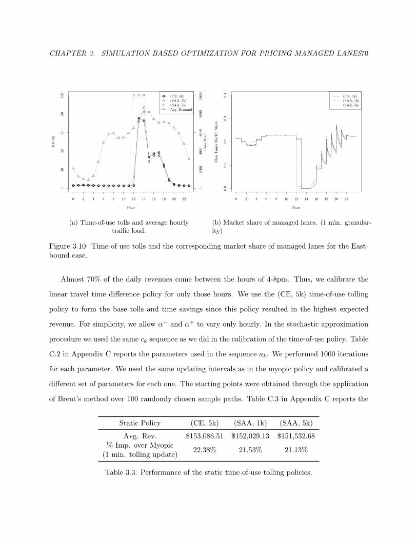
CHAPTER 3. SIMULATION BASED OPTIMIZATION FOR PRICING MANAGED LANES70
Hour
Tol
l ($
)
0 2 4 6 8 10 12 14 16 18 20 22
020
4060
8010
0
020
0040
0060
0080
0010
000
Car
s/H
our
(CE, 5k)(SAA, 1k)(SAA, 5k)Avg. Demand
(a) Time-of-use tolls and average hourlytraffic load.
Hour
Man
. L
anes
Mar
ket
Shar
e
0 2 4 6 8 10 12 14 16 18 20 22
0.0
0.1
0.2
0.3
0.4
(CE, 5k)(SAA, 1k)(SAA, 5k)
(b) Market share of managed lanes. (1 min. granular-ity)
Figure 3.10: Time-of-use tolls and the corresponding market share of managed lanes for the East-bound case.
Almost 70% of the daily revenues come between the hours of 4-8pm. Thus, we calibrate the
linear travel time difference policy for only those hours. We use the (CE, 5k) time-of-use tolling
policy to form the base tolls and time savings since this policy resulted in the highest expected
revenue. For simplicity, we allow α− and α+ to vary only hourly. In the stochastic approximation
procedure we used the same ck sequence as we did in the calibration of the time-of-use policy. Table
C.2 in Appendix C reports the parameters used in the sequence ak. We performed 1000 iterations
for each parameter. We used the same updating intervals as in the myopic policy and calibrated a
different set of parameters for each one. The starting points were obtained through the application
of Brent’s method over 100 randomly chosen sample paths. Table C.3 in Appendix C reports the
Static Policy (CE, 5k) (SAA, 1k) (SAA, 5k)
Avg. Rev. $153,086.51 $152,029.13 $151,532.68% Imp. over Myopic
22.38% 21.53% 21.13%(1 min. tolling update)
Table 3.3: Performance of the static time-of-use tolling policies.
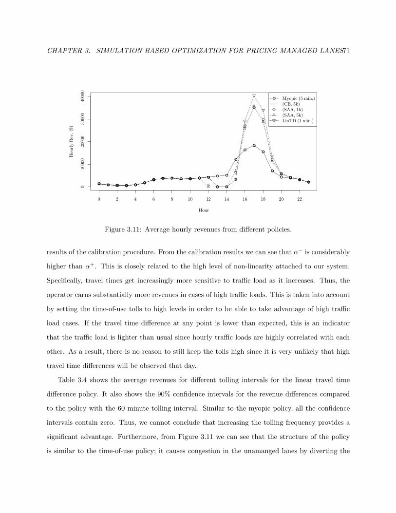
CHAPTER 3. SIMULATION BASED OPTIMIZATION FOR PRICING MANAGED LANES71
Hour
Hou
rly R
ev.
($)
0 2 4 6 8 10 12 14 16 18 20 22
010
000
2000
030
000
4000
0
Myopic (5 min.)(CE, 5k)(SAA, 1k)(SAA, 5k)LinTD (1 min.)
Figure 3.11: Average hourly revenues from different policies.
results of the calibration procedure. From the calibration results we can see that α− is considerably
higher than α+. This is closely related to the high level of non-linearity attached to our system.
Specifically, travel times get increasingly more sensitive to traffic load as it increases. Thus, the
operator earns substantially more revenues in cases of high traffic loads. This is taken into account
by setting the time-of-use tolls to high levels in order to be able to take advantage of high traffic
load cases. If the travel time difference at any point is lower than expected, this is an indicator
that the traffic load is lighter than usual since hourly traffic loads are highly correlated with each
other. As a result, there is no reason to still keep the tolls high since it is very unlikely that high
travel time differences will be observed that day.
Table 3.4 shows the average revenues for different tolling intervals for the linear travel time
difference policy. It also shows the 90% confidence intervals for the revenue differences compared
to the policy with the 60 minute tolling interval. Similar to the myopic policy, all the confidence
intervals contain zero. Thus, we cannot conclude that increasing the tolling frequency provides a
significant advantage. Furthermore, from Figure 3.11 we can see that the structure of the policy
is similar to the time-of-use policy; it causes congestion in the unamanged lanes by diverting the
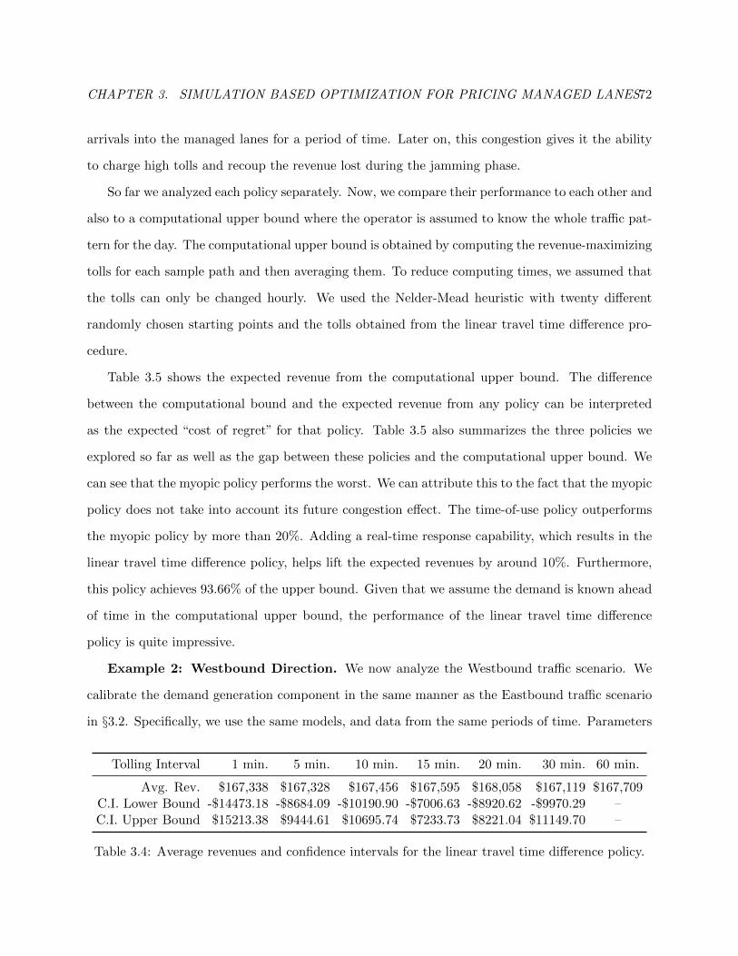
CHAPTER 3. SIMULATION BASED OPTIMIZATION FOR PRICING MANAGED LANES72
arrivals into the managed lanes for a period of time. Later on, this congestion gives it the ability
to charge high tolls and recoup the revenue lost during the jamming phase.
So far we analyzed each policy separately. Now, we compare their performance to each other and
also to a computational upper bound where the operator is assumed to know the whole traffic pat-
tern for the day. The computational upper bound is obtained by computing the revenue-maximizing
tolls for each sample path and then averaging them. To reduce computing times, we assumed that
the tolls can only be changed hourly. We used the Nelder-Mead heuristic with twenty different
randomly chosen starting points and the tolls obtained from the linear travel time difference pro-
cedure.
Table 3.5 shows the expected revenue from the computational upper bound. The difference
between the computational bound and the expected revenue from any policy can be interpreted
as the expected “cost of regret” for that policy. Table 3.5 also summarizes the three policies we
explored so far as well as the gap between these policies and the computational upper bound. We
can see that the myopic policy performs the worst. We can attribute this to the fact that the myopic
policy does not take into account its future congestion effect. The time-of-use policy outperforms
the myopic policy by more than 20%. Adding a real-time response capability, which results in the
linear travel time difference policy, helps lift the expected revenues by around 10%. Furthermore,
this policy achieves 93.66% of the upper bound. Given that we assume the demand is known ahead
of time in the computational upper bound, the performance of the linear travel time difference
policy is quite impressive.
Example 2: Westbound Direction. We now analyze the Westbound traffic scenario. We
calibrate the demand generation component in the same manner as the Eastbound traffic scenario
in §3.2. Specifically, we use the same models, and data from the same periods of time. Parameters
Tolling Interval 1 min. 5 min. 10 min. 15 min. 20 min. 30 min. 60 min.
Avg. Rev. $167,338 $167,328 $167,456 $167,595 $168,058 $167,119 $167,709C.I. Lower Bound -$14473.18 -$8684.09 -$10190.90 -$7006.63 -$8920.62 -$9970.29 –C.I. Upper Bound $15213.38 $9444.61 $10695.74 $7233.73 $8221.04 $11149.70 –
Table 3.4: Average revenues and confidence intervals for the linear travel time difference policy.

CHAPTER 3. SIMULATION BASED OPTIMIZATION FOR PRICING MANAGED LANES73
Policy Myopic (1 min.) (CE, 5k) LinTD (20 min.) Comp. Bound
Avg. Rev. $125,157 $153,087 $168,058 $179,444Rel. Gap 30.25% 14.69% 6.34% –
Table 3.5: Summary of policies and comparison to the computational upper bound.
for the demand model being utilized in this example can be found Appendix A. The data for
this direction was obtained through PeMS for VDS 1208151 and VDS 1208159 for managed and
unmanaged lanes, respectively. For simplicity, we used the consumer choice model 3-1 in Appendix
B in which both coefficients in the model do not vary over time. Similar to the previous example,
we generated 1000 sample paths for the traffic demand. In every case, unless stated otherwise, we
perform our analysis on the same set of sample paths.
In this section we compare and contrast the same set of policies. The starting tolls for the
stochastic approximation procedure are obtained by finding the revenue maximizing tolls for the
certainty equivalent demand case using the Nelder-Mead heuristic. In the stochastic approximation
procedure, we perform 1000 iterations and use the same set of sequences as we did in the Eastbound
case. Figure 3.12 depicts the average hourly demand, the time-of-use tolls we obtained through
stochastic approximation and the corresponding market share of managed lanes. Even though it is
not as severe as it was in the previous example, we can see that the time-of-use policy again seeks
to jam the unmanaged lanes by setting the toll very high between 6-7 am. As a result, the managed
lanes’ market share dips and most of the incoming cars choose the unmanaged lanes which in turn
causes congestion in the unmanaged lanes.
Our calibration methodology for the linear travel time difference policy is identical to the East-
bound case with a few minor differences. In contrast to the Eastbound scenario, traffic is more
evenly distributed throughout the day. So, we adjust the tolls for a wider range of hours, i.e. we
apply the linear travel time difference policy between the hours of 5 am and 7 pm. We apply the
same methodology as the previous example to obtain the starting points. We use the sequences
ck = 1/k1/6 and ak = 0.5/(200 + k), and perform 1000 iterations in the stochastic approximation
procedure. The resulting parameters can be found in Table C.4 of Appendix C.
The revenues obtained from different policies are given in Table 3.6. In line with the previous
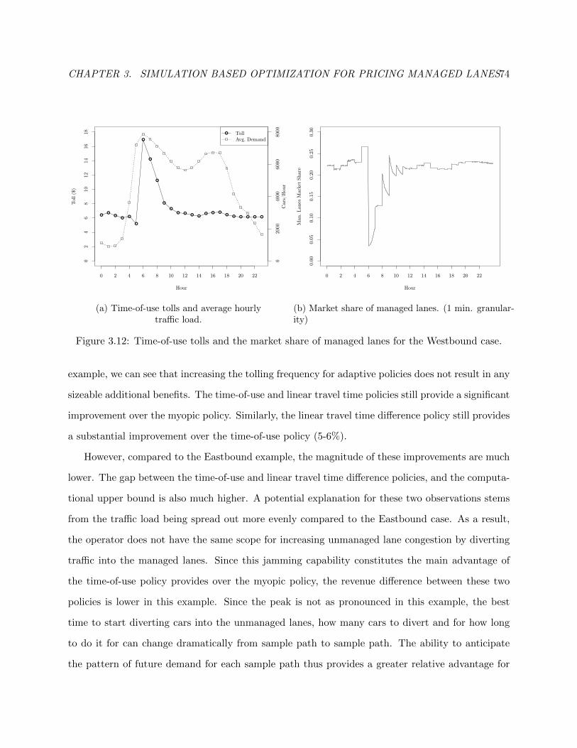
CHAPTER 3. SIMULATION BASED OPTIMIZATION FOR PRICING MANAGED LANES74
Hour
Tol
l ($
)
0 2 4 6 8 10 12 14 16 18 20 22
02
46
810
1214
1618
020
0040
0060
0080
00C
ars/
Hou
r
TollAvg. Demand
(a) Time-of-use tolls and average hourlytraffic load.
Hour
Man. L
anes
Mark
et
Share
0 2 4 6 8 10 12 14 16 18 20 22
0.0
00.0
50.1
00.1
50.2
00.2
50.3
0(b) Market share of managed lanes. (1 min. granular-ity)
Figure 3.12: Time-of-use tolls and the market share of managed lanes for the Westbound case.
example, we can see that increasing the tolling frequency for adaptive policies does not result in any
sizeable additional benefits. The time-of-use and linear travel time policies still provide a significant
improvement over the myopic policy. Similarly, the linear travel time difference policy still provides
a substantial improvement over the time-of-use policy (5-6%).
However, compared to the Eastbound example, the magnitude of these improvements are much
lower. The gap between the time-of-use and linear travel time difference policies, and the computa-
tional upper bound is also much higher. A potential explanation for these two observations stems
from the traffic load being spread out more evenly compared to the Eastbound case. As a result,
the operator does not have the same scope for increasing unmanaged lane congestion by diverting
traffic into the managed lanes. Since this jamming capability constitutes the main advantage of
the time-of-use policy provides over the myopic policy, the revenue difference between these two
policies is lower in this example. Since the peak is not as pronounced in this example, the best
time to start diverting cars into the unmanaged lanes, how many cars to divert and for how long
to do it for can change dramatically from sample path to sample path. The ability to anticipate
the pattern of future demand for each sample path thus provides a greater relative advantage for
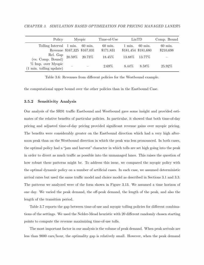
CHAPTER 3. SIMULATION BASED OPTIMIZATION FOR PRICING MANAGED LANES75
Policy Myopic Time-of-Use LinTD Comp. Bound
Tolling Interval 1 min. 60 min. 60 min. 1 min. 60 min. 60 min.Revenue $167,325 $167,031 $171,831 $181,454 $181,680 $210,698
Rel. Gap20.59% 20.73% 18.45% 13.88% 13.77% –
(vs. Comp. Bound)% Imp. over Myopic
– – 2.69% 8.44% 8.58% 25.92%(1 min. tolling update)
Table 3.6: Revenues from different policies for the Westbound example.
the computational upper bound over the other policies than in the Eastbound Case.
3.5.2 Sensitivity Analysis
Our analysis of the SR91 traffic Eastbound and Westbound gave some insight and provided esti-
mates of the relative benefits of particular policies. In particular, it showed that both time-of-day
pricing and adjusted time-of-day pricing provided significant revenue gains over myopic pricing.
The benefits were considerably greater on the Eastbound direction which had a very high after-
noon peak than on the Westbound direction in which the peak was less pronounced. In both cases,
the optimal policy had a “jam and harvest” character in which tolls are set high going into the peak
in order to divert as much traffic as possible into the unmanaged lanes. This raises the question of
how robust these patterns might be. To address this issue, we compared the myopic policy with
the optimal dynamic policy on a number of artificial cases. In each case, we assumed deterministic
arrival rates but used the same traffic model and choice model as described in Sections 3.1 and 3.3.
The patterns we analyzed were of the form shown in Figure 3.13. We assumed a time horizon of
one day. We varied the peak demand, the off-peak demand, the length of the peak, and also the
length of the transition period.
Table 3.7 reports the gap between time-of-use and myopic tolling policies for different combina-
tions of the settings. We used the Nelder-Mead heuristic with 20 different randomly chosen starting
points to compute the revenue maximizing time-of-use tolls.
The most important factor in our analysis is the volume of peak demand. When peak arrivals are
less than 9000 cars/hour, the optimality gap is relatively small. However, when the peak demand
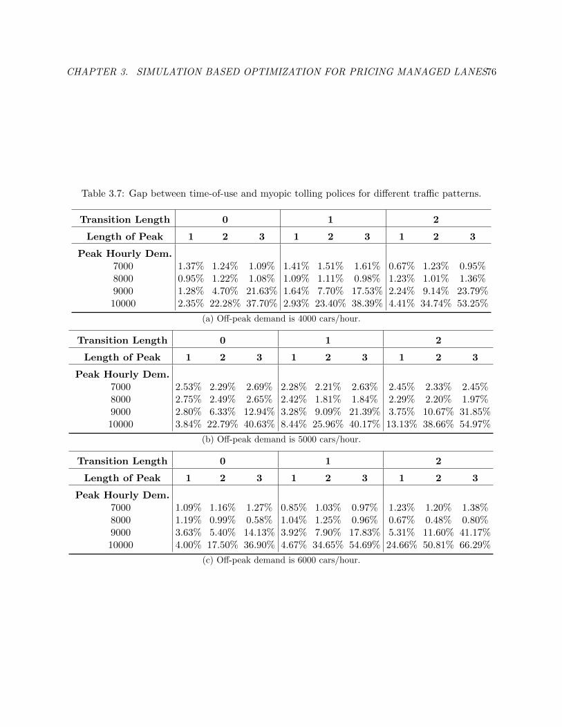
CHAPTER 3. SIMULATION BASED OPTIMIZATION FOR PRICING MANAGED LANES76
Table 3.7: Gap between time-of-use and myopic tolling polices for different traffic patterns.
Transition Length 0 1 2
Length of Peak 1 2 3 1 2 3 1 2 3
Peak Hourly Dem.7000 1.37% 1.24% 1.09% 1.41% 1.51% 1.61% 0.67% 1.23% 0.95%8000 0.95% 1.22% 1.08% 1.09% 1.11% 0.98% 1.23% 1.01% 1.36%9000 1.28% 4.70% 21.63% 1.64% 7.70% 17.53% 2.24% 9.14% 23.79%10000 2.35% 22.28% 37.70% 2.93% 23.40% 38.39% 4.41% 34.74% 53.25%
(a) Off-peak demand is 4000 cars/hour.
Transition Length 0 1 2
Length of Peak 1 2 3 1 2 3 1 2 3
Peak Hourly Dem.7000 2.53% 2.29% 2.69% 2.28% 2.21% 2.63% 2.45% 2.33% 2.45%8000 2.75% 2.49% 2.65% 2.42% 1.81% 1.84% 2.29% 2.20% 1.97%9000 2.80% 6.33% 12.94% 3.28% 9.09% 21.39% 3.75% 10.67% 31.85%10000 3.84% 22.79% 40.63% 8.44% 25.96% 40.17% 13.13% 38.66% 54.97%
(b) Off-peak demand is 5000 cars/hour.
Transition Length 0 1 2
Length of Peak 1 2 3 1 2 3 1 2 3
Peak Hourly Dem.7000 1.09% 1.16% 1.27% 0.85% 1.03% 0.97% 1.23% 1.20% 1.38%8000 1.19% 0.99% 0.58% 1.04% 1.25% 0.96% 0.67% 0.48% 0.80%9000 3.63% 5.40% 14.13% 3.92% 7.90% 17.83% 5.31% 11.60% 41.17%10000 4.00% 17.50% 36.90% 4.67% 34.65% 54.69% 24.66% 50.81% 66.29%
(c) Off-peak demand is 6000 cars/hour.

CHAPTER 3. SIMULATION BASED OPTIMIZATION FOR PRICING MANAGED LANES77
Figure 3.13: Demand pattern used in the sensitivity analysis.
passes that threshold, the gap increases substantially. As discussed in the traffic simulation section,
highway speeds are are quite insensitive to traffic loads up to a certain point. Once that threshold
is passed, however, speed is highly dependent on volume. When the peak demand stays below 9000
cars/hour, the unmanaged lanes have enough capacity to handle all the traffic flow without slowing
substantially. However, that is not the case when the peak demand rises to 9000 cars/hour. This
enables the controller to diver the traffic into the unmanaged lanes and reap the benefits from the
increased congestion as discussed in the previous section.
The influence of the number of transition periods, and the number of periods where the peak
demand is observed is clear once the peak demand is high. Similarly, the gap is also the most
sensitive to the peak demand when it is high. As all of these parameters increase, the static policy
has the capability of causing increasing levels of congestion in the unmanaged lanes. This increases
the attractiveness of the managed lanes further down the road, and gives the operator the ability
to charge tolls – much higher than the ones prescribed by the myopic policy.
3.5.3 Discussion
Our work provides a number of important insights into optimal managed lane tolling policies. First
of all, managing tolls around peaks – especially entering into the peak – is the most important aspect
of any revenue-maximizing policy. Secondly, optimal tolls have a “jam and harvest” character – by
charging high tolls entering into a peak period, they divert cars into the unmanaged lanes, thereby
increasing unmanaged lane congestion and enabling higher tolls later in the peak. Finally, when the

CHAPTER 3. SIMULATION BASED OPTIMIZATION FOR PRICING MANAGED LANES78
peak traffic is high relative to off-peak traffic, good heuristic policies can generate substantially more
revenue than the myopic policy. These observations are consistent with the results in Chapter 2. In
both of the dynamic policies we studied, increasing tolling frequency did not result in substantial
additional benefits. Thus, having the capability of updating the tolls frequently does not seem to
add a lot of value. A smart dynamic tolling mechanism potentially provides substantial revenue
improvements over a static time-of-use policy. However, we saw that such a policy does not need
to be very complex. What counts most is having the capability of sensing whether the traffic load
is higher than usual or not. A simple adaptive policy appears to be quite effective. Once it has
been calibrated, the linear travel time difference policy is quite simple to implement.
Our analysis assumed that all customers were tactical, that is that their arrival times are
exogenous and not dependent on either the tolls or the travel times. In actuality, some drivers may
have the flexibility to change their travel plans in order to avoid high tolls and/or high congestion.
Incorporation of such strategic behavior into the model might change the optimal tolls. However,
this would effectively require incorporating an equilibrium constraint into the model, which would
significantly increase its complexity. Furthermore, the persistence of highly predictable traffic jams
during certain periods shows that a very high number of travelers do not have great flexibility to
adjust their departure times.

CHAPTER 4. REVENUE MANAGEMENT OF CONSUMER OPTIONS FORTOURNAMENTS 79
Chapter 4
Revenue Management of Consumer
Options for Tournaments
This chapter is based on the paper “Revenue Management of Consumer Options for Tournaments”
which is a joint work with Santiago Balseiro, Prof. Robert Phillips and Prof. Guillermo Gallego.
This chapter diverts from the traffic theme of the previous two chapters. Instead, we focus on the
pricing of tournaments that utilize a different type of infrastructure (e.g., stadiums, tennis courts,
basketball courts). Unlike the previous chapters that focused on the pricing of a new infrastruc-
ture (the managed lanes), we analyze how an organizer can extract more revenue through the
introduction of a new product (consumer options) while utilizing the same existing infrastructure.
4.1 Model
We consider a tournament with N ≥ 3 teams, where there is uncertainty about the finalists. The
final is held in a venue with a capacity of C seats, which we assume of uniform quality. In the
case where the seats have heterogeneous quality, the stadium can be partitioned in sections, and
then each section can be considered independently. Alternatively, one could consider all sections
simultaneously using a nested revenue management model with upgrades (Gallego and Stefanescu,

CHAPTER 4. REVENUE MANAGEMENT OF CONSUMER OPTIONS FORTOURNAMENTS 80
2009).1
We address the problem of pricing and management of tickets and options for the final game.
The event manager offers N + 1 different products for the event: advance tickets, denoted by A
and options for each team i, denoted by Oi. Advance tickets require a payment of pa in advance
and guarantee a seat at the final game. An option Oi for team i is purchased at a price pio, and
confers the buyer a right to exercise and purchase the underlying ticket at a strike price pie only in
the event that team i advances to the final game. If the team fails to advance to the final game,
the option expires worthless and the premium paid is lost.
The event manager is a monopolist who can influence demand by varying the price. Hence, he
faces the problem of pricing the products and determining the number of products of each type
to offer so as to maximize his expected revenue. A common practice in sporting events is that
prices are announced in advance, and the organizer commits to those prices throughout the sales
horizon. We adhere to that static pricing practice in our model. However, the event manager does
not commit in advance to allocate a fixed number of seats for each product, and he can dynamically
react to demand by changing the set of products offered at each point in time.
For ease of exposition, the event manager is assumed to be risk-neutral, and performs no dis-
counting. Additionally, all costs incurred by the event manager are assumed to be sunk, so that
there is no marginal cost for additional tickets sold. From the event manager’s point of view seats
are perishable, that is, unsold seats have no value after the tournament starts since they cannot be
sold anymore. Finally, in agreement with current practice no overbooking is allowed in our model.
The timing of the events is as follows. First, the event manager announces the advance ticket’s
price pa, and the options’ premium and strike price (pio, pie) for each team i. Then, the box office
opens, and advance tickets and options are sold at those prices. Sales are allowed during a finite
horizon T that ends when the tournament starts. Afterwards, the tournament is played out, and
the two teams playing in the final are revealed. At this point the holders of options for the two
finalists decide whether to exercise their rights and redeem a seat at the corresponding strike price.
1In the model of Gallego and Stefanescu (2009) the event manager may upgrade customers to higher quality seats.Even though we do not pursue this direction in here, we note that upgrades help balance demand and supply byshifting excess capacity of high grade products to low grade products with excess demand.
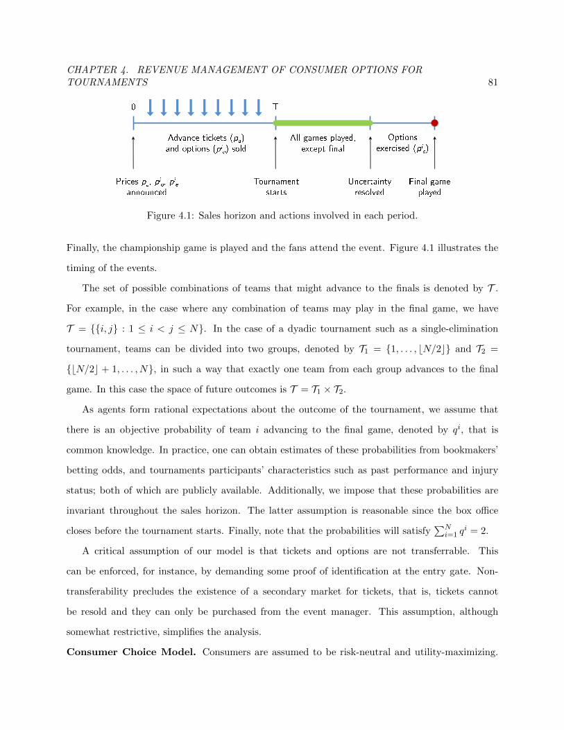
CHAPTER 4. REVENUE MANAGEMENT OF CONSUMER OPTIONS FORTOURNAMENTS 81
Figure 4.1: Sales horizon and actions involved in each period.
Finally, the championship game is played and the fans attend the event. Figure 4.1 illustrates the
timing of the events.
The set of possible combinations of teams that might advance to the finals is denoted by T .
For example, in the case where any combination of teams may play in the final game, we have
T = i, j : 1 ≤ i < j ≤ N. In the case of a dyadic tournament such as a single-elimination
tournament, teams can be divided into two groups, denoted by T1 = 1, . . . , bN/2c and T2 =
bN/2c + 1, . . . , N, in such a way that exactly one team from each group advances to the final
game. In this case the space of future outcomes is T = T1 × T2.
As agents form rational expectations about the outcome of the tournament, we assume that
there is an objective probability of team i advancing to the final game, denoted by qi, that is
common knowledge. In practice, one can obtain estimates of these probabilities from bookmakers’
betting odds, and tournaments participants’ characteristics such as past performance and injury
status; both of which are publicly available. Additionally, we impose that these probabilities are
invariant throughout the sales horizon. The latter assumption is reasonable since the box office
closes before the tournament starts. Finally, note that the probabilities will satisfy∑N
i=1 qi = 2.
A critical assumption of our model is that tickets and options are not transferrable. This
can be enforced, for instance, by demanding some proof of identification at the entry gate. Non-
transferability precludes the existence of a secondary market for tickets, that is, tickets cannot
be resold and they can only be purchased from the event manager. This assumption, although
somewhat restrictive, simplifies the analysis.
Consumer Choice Model. Consumers are assumed to be risk-neutral and utility-maximizing.
CHAPTER 4. REVENUE MANAGEMENT OF CONSUMER OPTIONS FORTOURNAMENTS 82
The demand is naturally segmented with respect to team preference, with N disjoint segments
corresponding to each team: we refer to consumers within segment i as fans of team i. In our
model, demand is stochastic and price sensitive, with customers arriving according to independent
Poisson processes with homogeneous intensity Λi for segment i. Time-dependent arrival intensities
can be handled by partitioning the sales horizon into intervals where the arrival rate is constant
(Liu and van Ryzin, 2008).
A fan of team i has two sources of utility, (i) attending a final game with his favorite team
playing, and (ii) attending the event when his team is not playing. The fan’s willingness-to-pay
for attending his favorite team’s final game, denoted by V , is drawn independently and at random
from a team-specific cumulative distribution function F iv(·). Fans do not update their valuations
over time, and as a result, expected utilities of the possible alternatives remain constant, which
means that the fans will not switch decisions, and there will be no cancellations or no-shows.
Furthermore, every option bought will be exercised. When his preferred team is not playing, the
fan is not sensitive to the finalists and will obtain only a fraction `i ∈ [0, 1] of his original valuation
if he watches the final. We refer to `i as the “love-of-the-game”; and it captures the fact that a fan’s
utility for attending a game without his preferred team is mostly influenced by his “love” for the
sport rather than by the identities of the actual finalists. In the extreme case when `i = 1, a fan’s
utility of attending the game is independent of whichever teams are playing. Conversely, when `i is
close to zero, fans have a strong preference towards their team, and are willing to attend the game
only if their team is playing. We shall see that the parameter `i turns out to be critical in our
model, and determines to a great extent the profitability of introducing options. The parameters
`i, F iv(·), and Λi are common knowledge.
At the moment of purchase, a fan of team i has three choices, (i) buy an advance ticket, (ii)
buy an option for his preferred team, or (iii) buy nothing. The first choice requires the payment
of the advance ticket price pa. Then, with probability qi, the fan expects to get a value of V
from seeing his team in the final and with probability 1 − qi he expects to get a value of `iV .
Hence, the fan’s expected utility for product A given a valuation of V , denoted by U ia(V ), is
U ia(V ) = (qi + (1− qi)`i)V − pa. The second choice, buying the option Oi, requires the payment of
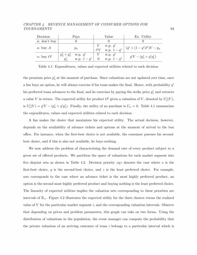
CHAPTER 4. REVENUE MANAGEMENT OF CONSUMER OPTIONS FORTOURNAMENTS 83
Decision Pays Value Ex. Utility
n: don’t buy 0 0 0
a: buy A paV w.p. qi
(qi + (1− qi)`i)V − pa`iV w.p. 1− qi
o: buy Oipio + pie w.p. qi V w.p. qi
qiV − (pio + qipie)pio w.p. 1− qi 0 w.p. 1− qi
Table 4.1: Expenditures, values and expected utilities related to each decision.
the premium price pio at the moment of purchase. Since valuations are not updated over time, once
a fan buys an option, he will always exercise if his team makes the final. Hence, with probability qi
his preferred team advances to the final, and he exercises by paying the strike price pie and extracts
a value V in return. The expected utility for product Oi given a valuation of V , denoted by U io(V ),
is U io(V ) = qiV − (pio + qipie). Finally, the utility of no purchase is Un = 0. Table 4.1 summarizes
the expenditures, values and expected utilities related to each decision.
A fan makes the choice that maximizes his expected utility. The actual decision, however,
depends on the availability of advance tickets and options at the moment of arrival to the box
office. For instance, when the first-best choice is not available, the consumer pursues his second-
best choice, and if this is also not available, he buys nothing.
We now address the problem of characterizing the demand rate of every product subject to a
given set of offered products. We partition the space of valuations for each market segment into
five disjoint sets as shown in Table 4.2. Decision priority xyz denotes the case where x is the
first-best choice, y is the second-best choice, and z is the least preferred choice. For example,
aon corresponds to the case where an advance ticket is the most highly preferred product, an
option is the second most highly preferred product and buying nothing is the least preferred choice.
The linearity of expected utilities implies the valuation sets corresponding to these priorities are
intervals of R+. Figure 4.2 illustrates the expected utility for the three choices versus the realized
value of V for the particular market segment i, and the corresponding valuation intervals. Observe
that depending on prices and problem parameters, this graph can take on two forms. Using the
distribution of valuations in the population, the event manager can compute the probability that
the private valuation of an arriving customer of team i belongs to a particular interval which is
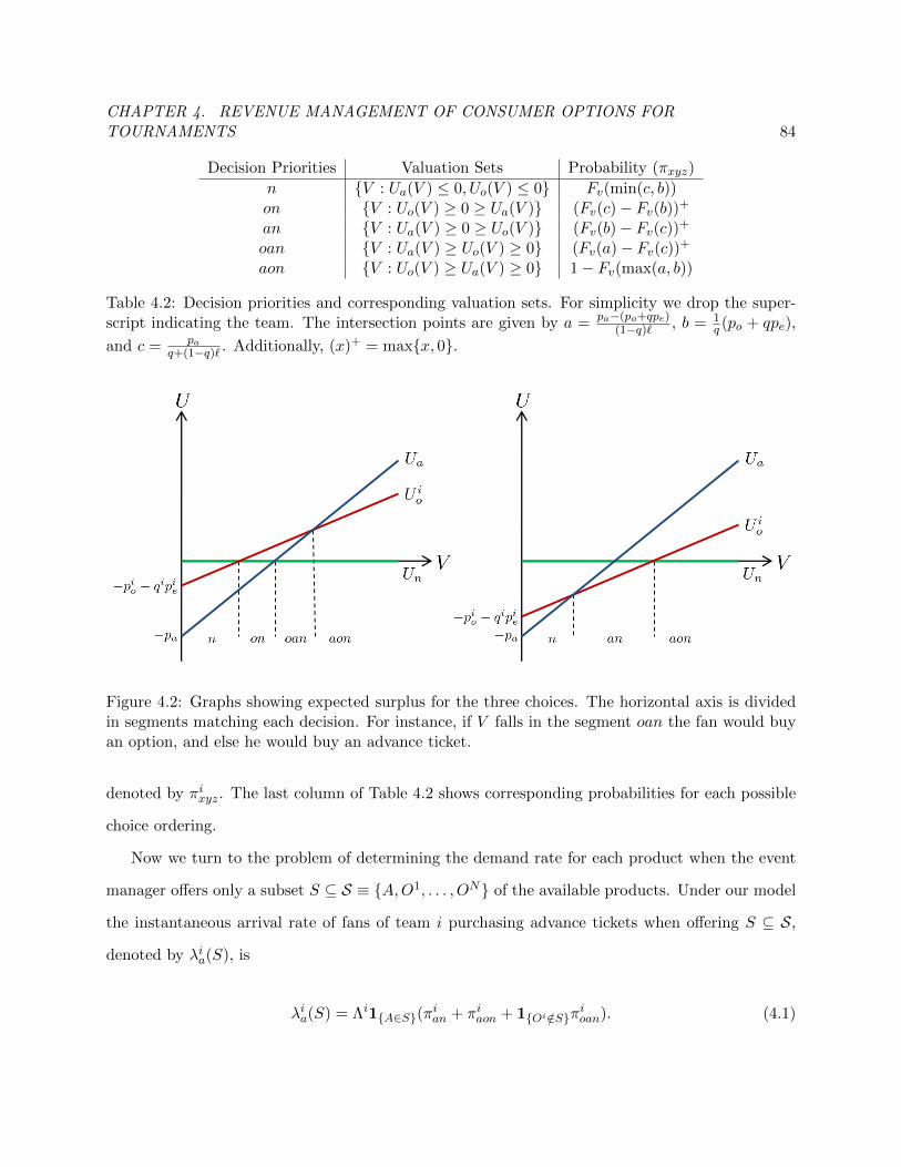
CHAPTER 4. REVENUE MANAGEMENT OF CONSUMER OPTIONS FORTOURNAMENTS 84
Decision Priorities Valuation Sets Probability (πxyz)
n V : Ua(V ) ≤ 0, Uo(V ) ≤ 0 Fv(min(c, b))on V : Uo(V ) ≥ 0 ≥ Ua(V ) (Fv(c)− Fv(b))+
an V : Ua(V ) ≥ 0 ≥ Uo(V ) (Fv(b)− Fv(c))+
oan V : Ua(V ) ≥ Uo(V ) ≥ 0 (Fv(a)− Fv(c))+
aon V : Uo(V ) ≥ Ua(V ) ≥ 0 1− Fv(max(a, b))
Table 4.2: Decision priorities and corresponding valuation sets. For simplicity we drop the super-script indicating the team. The intersection points are given by a = pa−(po+qpe)
(1−q)` , b = 1q (po + qpe),
and c = paq+(1−q)` . Additionally, (x)+ = maxx, 0.
Figure 4.2: Graphs showing expected surplus for the three choices. The horizontal axis is dividedin segments matching each decision. For instance, if V falls in the segment oan the fan would buyan option, and else he would buy an advance ticket.
denoted by πixyz. The last column of Table 4.2 shows corresponding probabilities for each possible
choice ordering.
Now we turn to the problem of determining the demand rate for each product when the event
manager offers only a subset S ⊆ S ≡ A,O1, . . . , ON of the available products. Under our model
the instantaneous arrival rate of fans of team i purchasing advance tickets when offering S ⊆ S,
denoted by λia(S), is
λia(S) = Λi1A∈S(πian + πiaon + 1Oi /∈Sπ
ioan). (4.1)
CHAPTER 4. REVENUE MANAGEMENT OF CONSUMER OPTIONS FORTOURNAMENTS 85
The arrival rate for advance ticket purchases is composed of three terms. The first term accounts
for fans that are only willing to buy those tickets. The second term accounts for fans that are
willing to buy the advance tickets, but when they are no longer available will buy the options as a
second choice. Finally, the third term considers fans that prefer options as their first choice, but
may end up buying advance tickets when options are not available. The aggregate arrival rate for
advance ticket purchases when offering subset S is λa(S) =∑N
i=1 λia(S). Similarly, the arrival rate
of fans of team i buying options when offering S, denoted by λio(S), is
λio(S) = Λi1Oi∈S(πion + πioan + 1A/∈Sπ
iaon). (4.2)
4.2 Pricing and Capacity Allocation Problem
In this section we look at the combined problem of pricing and managing advance tickets and options
faced by the organizer. Recall that prices are determined in advance, disclosed at the beginning
of the sales horizon, and remain constant thereon. However, the number of seats allocated to each
product are not disclosed in advance. The organizer can control the number of tickets and options
sold to dynamically react to the demand by playing with the availability of the products. Since the
resulting pricing and capacity allocation problem is intractable, we develop a novel approximation,
which we show to be asymptotically optimal when capacity and time are simultaneously scaled up.
Then, we conclude this section by addressing some of the practical issues that one might face in
the application of this approximation.
4.2.1 Problem Formulation
The sequential nature of the decisions involved suggests a partition of the problem into a two-stage
optimization problem. The decision variables are prices in the first stage and product availabilities
in the second stage. In the first stage, the organizer looks for the set of prices p = (pa, po, pe)
that maximizes the optimal value of the second-stage problem, which is the maximum expected
revenue that can be extracted under fixed prices p. This partition is well-defined because prices
CHAPTER 4. REVENUE MANAGEMENT OF CONSUMER OPTIONS FORTOURNAMENTS 86
are determined before the demand is realized, and are independent of the actual realization of the
demand. The optimal value of the first-stage problem, denoted by R∗, is
R∗ ≡ maxp≥0
R∗(p)
where R∗(p) denotes the optimal value of the second-stage problem.
The second-stage problem takes prices as given, and optimizes the expected revenue by con-
trolling the subset of products that is offered at each point in time. Notice that the second-stage
decision variable is a control policy over the offer sets, which is determined as the demand realizes.
We refer to this second-stage problem as the Capacity Allocation Problem. Next, we turn to the
problem of determining the optimal value of the second-stage problem under fixed prices p.
Once prices are fixed, the organizer attempts to maximize his revenue by implementing adaptive
non-anticipating policies that offer some subset S ⊆ S ≡ A,O1, . . . , ON of the available products
at each point in time. A control policy µ maps states of the system to control actions, i.e. the set of
offered products. We denote by Sµ(t) the subset of products offered under policy µ at time t. The
organizer can affect the arrival intensity of purchase requests by controlling the offer set Sµ(t). As
such, the total number of advance tickets sold up to time t is a non-homogeneous Poisson process
with arrival intensity λa(Sµ(t)) as defined in (4.1). We denote the event of an advance ticket being
sold at time t by dXa(Sµ(t)) = 1. Similarly, the number of options sold follow a non-homogenous
Poisson process with arrival intensity λio(Sµ(t)) as defined in (4.2), and we let dXio(Sµ(t)) = 1 when
an option is sold at time t. With some abuse of notation, we define Xa =∫ T
0 dXa(Sµ(t)) and
Xio =
∫ T0 dXi
o(Sµ(t)) to be the total number of advance tickets and options sold, respectively.
The second-stage or Capacity Allocation Problem can be formalized as the following stochastic

CHAPTER 4. REVENUE MANAGEMENT OF CONSUMER OPTIONS FORTOURNAMENTS 87
control problem which is similar to the one given in Liu and van Ryzin (2008):
R∗(p) = maxµ∈M
E
[paXa +
N∑i=1
(pio + qipie)Xio
]
s.t. Xa =
∫ T
0dXa(Sµ(t)), (4.3)
Xio =
∫ T
0dXi
o(Sµ(t)), ∀i = 1, . . . , N,
Xa +Xio +Xj
o ≤ C, (a.s.) ∀i, j ∈ T ,
where M is the set of all adaptive non-anticipating policies, and R∗(p) is the expected revenue
under the optimal policy µ∗. The first term in the objective accounts for the revenue from advance
ticket sales and the second term accounts for the revenue from options under the assumption that
all options are exercised, which was previously discussed in §4.1. Notice that because prices remain
constant during the time horizon, the expected revenue depends only on the expected number of
tickets sold. Unfortunately, this problem is very difficult to solve in most cases. The next section
gives a tractable and provably good deterministic approximation of (4.3).
4.2.2 Deterministic Approximation for the Second Stage Problem
In this section we follow Gallego et al. (2004), and solve a deterministic approximation of (4.3) in
which random variables are replaced by their means and quantities are assumed to be continuous.
We denote by ra = pa the expected revenue from selling an advance ticket, and by rio = pio + qipie
the expected revenue from selling an option of team i. Under this approximation, when a subset
of products S is offered, advance tickets (resp. options for team i) are purchased at a rate of
λa(S) (resp. λio(S)). Since ra (resp. rio) is the expected revenue from the sale of an advance ticket
(resp. option for team i), the rate of revenue generated from the sales of advance tickets is raλa(S)
(resp. rioλio(S) for options of team i). Additionally, because demand is deterministic and the choice
probabilities are time homogeneous, we only care about the total amount of time each subset of
products is offered and not the order in which they are offered. Thus, we only need to consider
the amount of time each subset S is offered, denoted by t(S), as the decision variables. Under this
CHAPTER 4. REVENUE MANAGEMENT OF CONSUMER OPTIONS FORTOURNAMENTS 88
notation, the number of advance tickets sold is∑
S⊆S t(S)λa(S), while the number of options sold
for team i is∑
S⊆S t(S)λio(S). Finally, the total revenue of the organizer is∑
S⊆S r(S)t(S), where
r(S) = rTλ(S) is the revenue rate when subset S is offered, and r =(ra, r
1o , . . . , r
No
)is the vector
of expected revenues.
Thus, we obtain the following choice-based deterministic LP model (CDLP):
RCDLP (p) ≡ maxt(S)
∑S⊆S
r(S)t(S) (4.4)
s.t.∑S⊆S
t(S) = T,
∑S⊆S
t(S)(λa(S) + λio(S) + λjo(S)
)≤ C, ∀i, j ∈ T (4.5)
t(S) ≥ 0 ∀S ⊆ S
where RCDLP (p) denotes the maximum revenue of the CDLP under prices p.
Since the linear program in (4.4) has one variable for each offer subset, it has 2N+1 variables in
total. For instance, if the tournament has 32 teams the program would have more than 8 billion
variables! Fortunately, by exploiting the structure of our choice model it is possible to derive an
alternative formulation with a linear number of variables and constraints.
Recall that consumers are partitioned into N different market segments, each associated with
a different team. Two different products are potentially offered to each segment i = 1, . . . , N : (i)
advance tickets (A) and (ii) options for the associated team (Oi). We denote by Si = A,Oi the
set of products available for market segment i. Demands across segments are independent, and
different segments are only linked through the capacity constraints. Since each segment has two
products, only four offer sets need to be considered. Thus, for each market segment we only need
the following decision variables: (i) the time both advance tickets and options are offered, denoted
by ti(A,Oi
), (ii) the time only advance tickets are offered, denoted by ti (A), (iii) the time
only options are offered, denoted by ti(Oi
), and (iv) the time no product is offered, denoted by
ti (∅). Given a solution t(S)S⊆S for the CDLP, the value of the new decision variables can be

CHAPTER 4. REVENUE MANAGEMENT OF CONSUMER OPTIONS FORTOURNAMENTS 89
computed as follows
ti(S) =∑
S′⊆S:S′∩Si=S
t(S′). (4.6)
Observe that for each segment offer times should sum up to length of the horizon, that is∑S⊆Si t
i(S) = T . An important observation is that by requiring∑
S⊆Si\∅ ti(S) ≤ T we do not
need to keep track of the time in which no product is offered for each segment. Additionally,
in order for the offer sets to be consistent across market segments, the total time that advance
tickets are offered should be equal for all segments, i.e., for some Ta ≥ 0 it should be the case that
ti(A,Oi
)+ ti (A) = Ta for all i = 1, . . . , N where Ta denotes the total time advance tickets are
offered throughout the sales horizon.
After applying the aforementioned changes, we obtain the following market-based deterministic
LP (MBLP)
RMBLP (p) ≡ maxti(S),Ta
N∑i=1
∑S⊆Si
ri(S)ti(S) (4.7)
s.t.∑S⊆Si
ti(S) ≤ T ∀i = 1, . . . , N (4.8)
ti(A,Oi
)+ ti (A) = Ta ∀i = 1, . . . , N (4.9)
N∑k=1
∑S⊆Sk
tk(S)λka(S)
+∑S⊆Si
ti(S)λio(S) +∑S⊆Sj
tj(S)λjo(S) ≤ C ∀i, j ∈ T (4.10)
Ta ≥ 0, ti(S) ≥ 0 ∀S ⊆ Si, i = 1, . . . , N,
where ri(S) = paλia(S) + rioλ
io(S) is the revenue rate from market segment i when subset S ⊆ Si is
offered. Notice that the new optimization problem has 3N + 1 variables, which is much less than
CDLP, and O(N2) constraints.
Proposition 1. The MBLP is equivalent to the CDLP, i.e. RMBLP (p) = RCDLP (p) for all prices

CHAPTER 4. REVENUE MANAGEMENT OF CONSUMER OPTIONS FORTOURNAMENTS 90
p ≥ 0.
Proof: We first show that RCDLP (p) ≤ RMBLP (p) by showing that any solution of the CDLP can
be used to construct a feasible solution to the MBLP with the same objective value. Let t(S)S⊆S
be a feasible solution to the CDLP. First, using the decision variables given by (4.6), the total
number of advance tickets sold can be written as
Xa =∑S⊆S
t(S)λa(S) =∑S⊆S
t(S)N∑i=1
Λi1A∈S(πian + πiaon + 1Oi /∈Sπ
ioan)
=
N∑i=1
( ∑S⊆S:A∈S,Oi∈S
t(S))
Λi(πian + πiaon) +( ∑S⊆S:A∈S,Oi 6∈S
t(S))
Λi(πian + πiaon + πioan)
=N∑i=1
ti(A,Oi
)λia(A,Oi
)+ ti (A)λia (A) =
N∑i=1
∑S⊆Si
ti(S)λia(S), (4.11)
where the second equality follows from (4.1), the third from exchanging summations, and the fourth
from (4.1) again. Similarly, the number of options sold in market segment i can be written as
Xio =
∑S⊆S
t(S)λio(S) =∑S⊆S
t(S)Λi1Oi∈S(πion + πioan + 1A/∈Sπ
iaon
)=( ∑S⊆S:A∈S,Oi∈S
t(S))
Λi(πion + πioan) +( ∑S⊆S:A∈S,Oi 6∈S
t(S))
Λi(πion + πioan + πiaon)
= ti(A,Oi
)λio(A,Oi
)+ ti (A)λio (A) =
∑S⊆Si
ti(S)λio(S), (4.12)
where the second equality follows from (4.2), the third from exchanging summations, and the fourth
from (4.2) again. Thus, the capacity constraint (4.10) is verified.
The non-negativity constrains and the time-horizon length constraints (4.8) follow trivially.
Next, for the advance selling market consistency constraints (4.9) notice that for all i = 1, . . . , N
we have that
ti(A,Oi
)+ ti (A) =
∑S⊆S:A∈S,Oi∈S
t(S) +∑
S⊆S:A∈S,Oi 6∈S
t(S) =∑
S⊆S:A∈St(S) = Ta.

CHAPTER 4. REVENUE MANAGEMENT OF CONSUMER OPTIONS FORTOURNAMENTS 91
Thus, advance tickets are offered the same amount of time in all markets.
Finally, the next string of equalities show that both solutions attain the same objective value
∑S⊆S
r(S)t(S) =∑S⊆S
rTλ(S)t(S) =∑S⊆S
N∑i=1
(raλ
ia(S) + rioλ
io(S)
)t(S)
=N∑i=1
∑S⊆Si
raλia(S)ti(S) + rioλ
io(S)ti(S) =
N∑i=1
∑S⊆Si
ri(S)ti(S),
where the third equality follows from (4.11) and (4.12).
Next, we show that RCDLP (p) ≥ RMBLP (p) by showing that any solution of the MBLP
can be used to construct a feasible solution to the CDLP with the same objective value. Letti(S)
S⊆Si,i=1,...,N
be a feasible solution to the MBLP. In the following, we give a simple algo-
rithm to compute a feasible solution t(S)S⊆S for the CDLP.
First, we deal with offer sets containing advance tickets, and compute t(S) for all S ∈ S such
that A ∈ S. Let [i]i=1,...,N be the permutation in which teams are sorted in increasing order with
respect to ti(A,Oi
), i.e. t[i]
(A,O[i]
)≤ t[i+1]
(A,O[i+1]
). Consider the following offer sets
S[i] =A,O[i], O[i+1], . . . , O[N ]
∀i = 1, . . . , N
S[N+1] = A
and associated times t(S[i])
= t[i](A,O[i]
)− t[i−1]
(A,O[i−1]
)for all i = 1, . . . , N + 1, with
t[0](A,O[0]
)= 0, and t[N+1]
(A,O[N+1]
)= Ta. Since teams are sorted with respect to
ti(A,Oi
), we have t
(S[i])≥ 0. Notice that this construction is valid because the market consis-
tency constraints (4.9) guarantee that advance tickets are offered the same amount of time in all
markets. Figure 4.3 sketches a graphical representation of the algorithm.
Next, we look at the intuition behind this construction. Although the order is not important,
consider a solution for the CDLP that offers the sets S[i] in sequential order; it starts with S[1],
then S[2], and so forth until S[N+1]. Hence, at first it offers all products, then team 1’s options are
removed, then team 2’s options are removed, and so forth until the end when only advance tickets
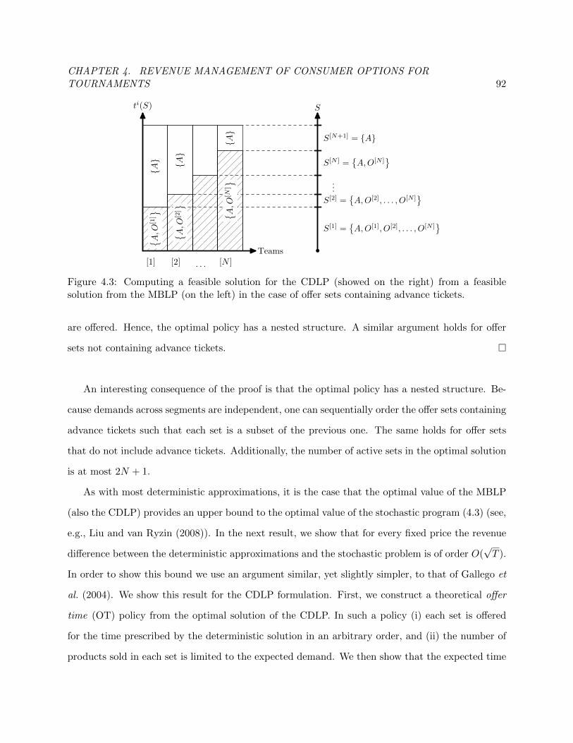
CHAPTER 4. REVENUE MANAGEMENT OF CONSUMER OPTIONS FORTOURNAMENTS 92
S[1] =A,O[1], O[2], . . . , O[N ]
S[2] =
A,O[2], . . . , O[N ]
...
S[N ] =A,O[N ]
S[N+1] = A
A,O
[1]
A
[1]
A,O
[2]
A
[2] . . .
A,O
[N]
A
[N ]Teams
ti(S) S
Figure 4.3: Computing a feasible solution for the CDLP (showed on the right) from a feasiblesolution from the MBLP (on the left) in the case of offer sets containing advance tickets.
are offered. Hence, the optimal policy has a nested structure. A similar argument holds for offer
sets not containing advance tickets.
An interesting consequence of the proof is that the optimal policy has a nested structure. Be-
cause demands across segments are independent, one can sequentially order the offer sets containing
advance tickets such that each set is a subset of the previous one. The same holds for offer sets
that do not include advance tickets. Additionally, the number of active sets in the optimal solution
is at most 2N + 1.
As with most deterministic approximations, it is the case that the optimal value of the MBLP
(also the CDLP) provides an upper bound to the optimal value of the stochastic program (4.3) (see,
e.g., Liu and van Ryzin (2008)). In the next result, we show that for every fixed price the revenue
difference between the deterministic approximations and the stochastic problem is of order O(√T ).
In order to show this bound we use an argument similar, yet slightly simpler, to that of Gallego et
al. (2004). We show this result for the CDLP formulation. First, we construct a theoretical offer
time (OT) policy from the optimal solution of the CDLP. In such a policy (i) each set is offered
for the time prescribed by the deterministic solution in an arbitrary order, and (ii) the number of
products sold in each set is limited to the expected demand. We then show that the expected time
CHAPTER 4. REVENUE MANAGEMENT OF CONSUMER OPTIONS FORTOURNAMENTS 93
each set is offered in the OT policy is close to the the deterministic solution, and then conclude
that the performance of such a policy is close to the deterministic upper bound.
Theorem 1. Fix prices p ≥ 0. Let t∗(S)S∈S be an optimal solution for the CDLP for the given
prices, and S∗ = S ∈ S : t∗(S) > 0 be the subsets of products with positive offer times in the
optimal solution. Then, then the revenue loss of the stochastic control problem with respect to the
CDLP is bounded by
0 ≤ RCDLP (p)−R∗(p) ≤ rmax|S∗|(λ−1
min +√
(N + 1)λ−1minT
),
where rmax is the maximum revenue rate among all products available in the offer sets in S∗.
Similarly, λmin be the minimum arrival rate among all products available in the offer sets in S∗. 2
Proof: Fix prices p. The first bound follows from Proposition 1 in Liu and van Ryzin (2008),
which they proved by using the optimal policy µ∗ of the stochastic control problem to construct
a candidate solution for the CDLP. In the candidate solution each set is offered for an amount of
time tµ∗(S) = E[∫ T
0 1Sµ∗(t) = S dt]. Such a solution is easily shown to be feasible for the CDLP
and attains the same objective value as the original stochastic problem. Thus, one concludes that
R∗(p) ≤ RCDLP (p) since every solution of the CDLP is upper bounded by its optimal value.
In order to show the second bound we use an argument similar to that of Gallego et al. (2004).
First, we construct a theoretical offer time (OT) policy from the optimal solution of the CDLP. In
such a policy one offers each set for the time prescribed by the deterministic solution in an arbitrary
order. Additionally, the number of products sold in each set is limited to the expected demand,
and each set is offered until either the time or any of the products run out. We denote by ROT (p)
to be the expected revenue of the offer time control. Clearly, it is the case that ROT (p) ≤ R∗(p).
We shall bound the difference between ROT (p) and the upper bound RCDLP (p).
We construct the OT policy as follows. Let t∗(S) be the optimal solution of the CDLP. With
some abuse of notation we refer to advance tickets as the zero option, i.e., A ≡ O0, Xa ≡ X0o ,
2Let A ≡ O0 and pa ≡ r0o. Then, rmax = maxS⊆S∗,Oi∈Srio(S) be the maximum revenue rate and λmin =
minS⊆S∗,Oi∈Sλio(S) be the minimum arrival rate.

CHAPTER 4. REVENUE MANAGEMENT OF CONSUMER OPTIONS FORTOURNAMENTS 94
pa ≡ r0o , and λa(S) ≡ λ0
o(S). Under the OT policy, set S is offered for a time τOT (S)d=
mint∗(S),minOi∈S τio(S), where τ io(S) is the first time we run out of options for team ith in
an alternate system in which products are sold independently of each other. More formally, we
have that
τ io(S) = inft : Xio(S, t) ≥ bλio(S)t∗(S)c,
options sold by time t when offering set S in the alternate system, and bxc is largest integer not
greater than x. For the sake of simplicity we assume that the limits on the number of tickets sold
are stricly positive, else they can be excluded from the offer set. Notice that τ io(S) is an Erlang
random variable with rate λio(S) and shape parameter bλio(S)t∗(S)c.
Before proceeding we state some definitions. Let rmax = maxS⊆S∗,Oi∈Srio(S) be the maximum
revenue rate and λmin = minS⊆S∗,Oi∈Sλio(S) be the minimum arrival rate.
We can lower bound the expected value of the random time τOT (S) using the bound for the
minimum of random variables from Aven (1985) by
E[τOT (S)
]≥ mint∗(S), min
Oi∈SE[τ io(S)] −
√√√√ |S||S|+ 1
∑Oi∈S
Var [τ io(S)]
≥ t∗(S)− maxOi∈S
λio(S)−1 −√t∗(S)
∑Oi∈S
λio(S)−1
≥ t∗(S)− λ−1min −
√t∗(S)(N + 1)λ−1
min,
where the second inequality follows from the fact that E[τ io(S)
]= bλio(S)t∗(S)c/λio(S) ≥ t∗(S) −
1/λio(S), and Var[τ io(S)
]= bλio(S)t∗(S)c/λio(S)2 ≤ t∗(S)/λio(S).
Next, we bound the expected revenue of the offer time policy. Using the fact that τOT (S) is a

CHAPTER 4. REVENUE MANAGEMENT OF CONSUMER OPTIONS FORTOURNAMENTS 95
bounded stopping time together with the previous bound we obtain that
ROT (p) = E
∑S⊆S
∑Oi∈S
rioXio(S, τ
OT (S))
=∑S⊆S
∑Oi∈S
rioλio(S)E
[τOT (S)
]≥∑S⊆S
r(S)t∗(S)−∑S⊆S
r(S)(λ−1min +
√t∗(S)(N + 1)λ−1
min)
≥ RCDLP (p)− rmaxλ−1min|S
∗| − rmax
√(N + 1)λ−1
min
∑S⊆S
√t∗(S)
≥ RCDLP (p)− rmax|S∗|(λ−1
min +√
(N + 1)λ−1min
√T
),
where the last inequality follows from the fact that∑
S⊆S√t∗(S) ≤ |S∗|
√∑S⊆S t
∗(S). Note that
the OT policy, in spite of its simplicity, is asymptotically optimal for the stochastic control problem.
As a corollary, we get that the CDLP becomes asymptotically optimal as the stadium capacity
and length of the time horizon are simultaneously scaled up. To see this, let R∗θ(p) be the optimal
objective of a scaled stochastic problem in which capacity is set to θC and time horizon to θT for
some θ ≥ 1. Similarly, let RCDLPθ (p) be the optimal objective of a scaled CDLP. Notice that the
CDLP is insensitive to the scaling, that is, 1θR
CDLPθ (p) = RCDLP (p). Then from Theorem 1 one
gets that the CDLP is asymptotically optimal for the second-stage problem, or equivalently 1θR∗θ(p)
converges to RCDLP (p) as θ →∞ for all p ≥ 0. Moreover, it is not hard to see that the asymptotic
optimality of the CDLP carries over to the first-stage problem. Solving the CDLP instead of the
stochastic control in the second-stage is asymptotically optimal for the first-stage problem.
4.2.3 Implementation and Practical Considerations
As we previously discussed, the optimal value of the capacity allocation problem R∗(p) is hard
to compute. Hence, in order to tackle our problem, we replace the objective of the first-stage
problem with the upper-bound provided by the deterministic approximation RMBLP (p). This new
problem provides an upper bound to the truly optimal objective value R∗. However, in view of

CHAPTER 4. REVENUE MANAGEMENT OF CONSUMER OPTIONS FORTOURNAMENTS 96
the asymptotic optimality of the deterministic approximation, and the large scale of the problem
in terms of stadium’s capacity, our policy is expected to perform reasonably well.
Using our approximation for the second-state problem, the first-stage problem amounts to
optimizing the non-linear function RMBLP (p) over the polyhedron of prices. Because the objective
is not necessarily convex as a function of price, multiple different starting points need to be taken.
Given our efficient method to evaluate the approximate objective value of the capacity allocation
problem, we are able to find good solutions for real problems of moderate size despite the non-
convexity of the objective.
After the optimal solution is computed, a remaining issue is how tickets should be sold. Clearly,
the event manager should announce the optimal prices p∗ at the beginning, and commit to that
price throughout the sales horizon. However, one important issue is the capacity allocation of the
tickets, and constructing a good dynamic control policy from the output of the approximation. The
optimal solution of the deterministic approximation prescribes only how long each subset should
be offered, but does not specify how to implement the actual policy. One straightforward approach
is to offer each subset S for the amount of time given by t(S). As pointed out by Liu and van
Ryzin (2008), this approach has a few problems. First, the order in which the sets are offered is
not specified, and the resulting policy is static and does not react to changes in demand.
Various heuristics have been proposed to address the first problem. Liu and van Ryzin (2008)
proposed a decomposition approach in which the dual optimal solutions of the deterministic problem
are used to decompose the network dynamic program into a collection of leg-level DPs which can
be solved exactly. These are then used to construct a control policy. Kunnumkal and Topaloglu
(2010) improved upon this idea by considering an alternative dynamic programming decomposition
method that performs the allocations by solving an auxiliary optimization problem. Alternatively,
Zhang and Adelman (2006) employ an approximate dynamic programming scheme in which the
value function is approximated with affine functions of the state vector. This allows them to obtain
dynamic bid-prices that are later used to construct control policies.
Inspired by our efficient formulation, we propose a simple sales limit policy. The policy offers all
tickets from the beginning, and limits the number of each product sold to the expected value given
CHAPTER 4. REVENUE MANAGEMENT OF CONSUMER OPTIONS FORTOURNAMENTS 97
by the deterministic approximation. That is, tickets are sold either until the end of horizon or the
limit is reached, whichever happens first. The limits are given by Xa for the advance tickets, and
Xio for the ith team options. This policy is not guaranteed to be optimal, but performs surprisingly
well. Two attractive features of this policy are its ease of implementation, and the fact that it
concurs with the current sales practice.
To address the static nature of the control policy, one could periodically resolve the deterministic
approximation. Recently, Jasin and Kumar (2010) showed that carefully chosen periodic resolving
schemes together with probabilistic allocation controls can achieve a bounded revenue loss w.r.t. the
optimal online policy (static control policies are guaranteed to achieve a revenue loss that grows as
the squared root of the size of the problem). We do not pursue this direction in here, but note that
one could attempt to periodically resolve the MBLP to improve the performance.
4.3 The Symmetric Case
In this section we consider a symmetric version of the problem that has the following character-
istics, (i) all teams have the same probability of advancing to the final, (ii) arrival rates are the
same for all teams, (iii) valuations are i.i.d. across teams, and (iv) the love-of-the-game is constant
throughout the population. These assumptions, albeit not entirely realistic, allows us to theoreti-
cally characterize the benefits of introducing options. As we shall later see in the numerical analysis
part, the conditions under which options are beneficial frequently carry over to the most general
case.
The following analysis will be based on the deterministic approximation of the problem and
not the actual stochastic performance. Due to the asymptotic optimality of the deterministic
approximation and the large scale of the problem, it should be expected that these results carry
over to the fully stochastic setting.
We start this section by first formulating the ticket pricing problem for the symmetric case.
Then, we show that offering options increases the revenue of the organizer, and also provide bounds
on the revenue improvement. Lastly, we analyze the social efficiency of offering options.
CHAPTER 4. REVENUE MANAGEMENT OF CONSUMER OPTIONS FORTOURNAMENTS 98
4.3.1 Advance Ticket and Options Pricing Problem
In a symmetric problem with N teams, each team has the same probability q = 2N of advancing
to the final game. The arrival rate of fans of each team is λ = ΛN , where Λ denotes the aggregate
arrival rate. Due to the symmetry of the teams, we look for solutions in which the organizer charges
the same expected price ro = po+qpe for options for all teams. Hence, we will sell the same number
of options to all teams.
The aggregate arrival intensity of advance tickets and options under prices pa and ro can be
computed as
λa(pa, ro) = ΛFv
(pa − ro(1− q)`
),
λo(pa, ro) = Λ
[Fv
(roq
)− Fv
(pa − ro(1− q)`
)],
where we denote by λo the aggregate arrival intensity of all consumers buying options. We assume
that the c.d.f. of the values Fv(·) is continuous and strictly increasing. Thus, there is a one-to-one
correspondence between prices and arrival rates, and the inverse functions are given by
ro(λa, λo) = qFv−1(λa + λo
Λ
),
pa(λa, λo) = qFv−1(λa + λo
Λ
)+ (1− q)`Fv−1
(λaΛ
).
The one-to-one correspondence between prices and arrival intensity allows us to recast the
problem with the arrival intensities as the decision variables; the promoter determines target sales
intensities λa and λo and the market determines the prices based on this quantity. Under this
change of variables, the deterministic approximation of the advance ticket and options pricing
CHAPTER 4. REVENUE MANAGEMENT OF CONSUMER OPTIONS FORTOURNAMENTS 99
problem becomes
RDo = maxλa≥0,λo≥0
T (1− q)`v(λa) + Tqv(λa + λo) (4.13a)
s.t. Tλa + T2
Nλo ≤ C, (4.13b)
λa + λo ≤ Λ,
where we have written the objective in terms of the value rate v(λa) = λaFv−1 (λa
Λ
).
In the following, we assume that the value rate is regular and differentiable. Regularity implies
that v(·) is continuous, bounded, concave, satisfies limλa→0 v(λa) = 0, and has a least maximizer
λ∗a. These assumptions are common in the RM literature (see, e.g., Gallego and van Ryzin (1994)).
A sufficient condition for the concavity of the value rate is that valuations have increasing failure
rate (IFR), or equivalently that the failure rate of values as given by h(x) = fv(x)/Fv(x) is non-
decreasing. A consequence of regularity is that the objective of program (4.13) is concave. Hence,
(4.13) is a concave maximization problem with linear inequality constraints. Additionally, because
the objective is continuous and the feasible set is compact, by Weierstrass’ Theorem, there exists
an optimal solution (Luenberger, 1969).
We are now in a position to characterize some conditions under which options are beneficial
to the organizer. In the following we denote by RDa the optimal revenue of the deterministic
approximation for the organizer when only advance tickets are sold, which amounts to setting
λo = 0 in program (4.13).
Theorem 2. In the symmetric case, when the seats are scarce (C < λ∗aT ) and fans strictly prefer
their own team (` < 1), introducing options increases the revenue of the organizer (RDo > RDa ).
However, when the capacity of the stadium is large (C ≥ λ∗aT ) or fans are indifferent among teams
(` = 1) options do not increase the revenue.
Proof: Recall that the deterministic approximation of the advance ticket pricing problem is equal
to the option pricing problem (4.13) under the condition that λo = 0. This can be equivalently
CHAPTER 4. REVENUE MANAGEMENT OF CONSUMER OPTIONS FORTOURNAMENTS 100
written as
RDa = maxλa≥0
T (q + (1− q)`) v(λa) (4.14)
s.t. Tλa ≤ C, λa ≤ Λ.
We write the gradient of the option pricing problem objective
∂RDo∂λo
= Tqv′(λa + λo),
∂RDo∂λa
= T (1− q)`v′(λa) + Tqv′(λa + λo).
First, we look at the case where the seats are scarce (C < λ∗aT ). In the advance ticket pricing
problem (4.14) the organizer can afford to price higher, and prices at the run-out rate λ0a = C/T ,
i.e., the intensity at which all seats are sold over the time horizon. Note that λ0a is a constrained
global optimum of the advance selling problem, and v′(λ0a) > 0. Starting from (λ0
a, 0) in the options
pricing problem, we will study the impact of increasing the options’ intensity on the revenue.
Clearly, (λ0a, 0) is a feasible solution of (4.13). Since capacity is binding, to compensate for an
increase in λo the organizer needs to decrease the intensity of advance tickets. Thus, from (4.13b)
we obtain that dλadλo
= − 2N = −q. Evaluating the total derivative of the objective at (λ0
a, 0) we
obtain
dRDodλo
=∂RDo∂λo
+∂RDo∂λa
dλadλo
= Tqv′(λ0a)− Tq ((1− q)`+ q) v′(λ0
a)
= Tq(1− q)(1− `)v′(λ0a) > 0.
This implies that the current solution can be improved by introducing except when ` = 1, in which
case there is no benefit from selling options.
Second, we consider the case where the capacity of the stadium is large (C ≥ λ∗aT ). In the
advance ticket pricing problem (4.14) the organizer ignores the problem of running out of seats

CHAPTER 4. REVENUE MANAGEMENT OF CONSUMER OPTIONS FORTOURNAMENTS 101
and prices according to the revenue maximizing rate λ∗a. Note that λ∗a is an unconstrained global
optimum, and thus v′(λ∗a) = 0. Clearly, (λ∗a, 0) is a feasible solution of (4.13), and the gradient
of the objective is zero at (λ∗a, 0) since v′(λ∗a) = 0. Hence, this solution is an unconstrained lo-
cal optimum and the concavity of the program implies this is also a global optimum. Thus, the
current solution cannot be improved by introducing options and this result is independent of `.
The previous result shows that options are beneficial for the event manager only when the
demand is high with respect to the stadium’s capacity and fans strictly prefer their own team over
any other. In the case that fans are indifferent among teams (` = 1), the result is trivial since
consumers strictly prefer advance tickets over options. The most interesting case is when fans
strictly prefer their own team over any other (` < 1). From the point of view of a consumer, the
main difference between the products is that an advance ticket allows him to attend the final game
even when his favorite team is not playing, providing an extra source of utility. Therefore, if both
products have the same expected cost, a risk-neutral consumer would choose an advance ticket
over an option. When capacity is abundant, the organizer can ignore the problem of running out
of seats, and for the same expected revenue per product sold he can elicit a stronger demand for
advance tickets. Thus, in this case the introduction of options is not beneficial for the organizer.
However, when capacity is scarce the organizer should balance the expected revenue and the
expected capacity consumed for each unit of product sold. While each advance ticket consumes
exactly one seat, options from different teams can be assigned to the same seat, which allows the
organizer to effectively sell more than one option per unit of capacity. Even though at most one
fan will exercise the option assigned to that seat, the organizer gets to keep the premiums paid
by the other consumers. Thus, when capacity is scarce, there are two conflicting effects associated
to the introduction of options. On one hand, consumers buy options only when the expected cost
of an option is less than that of an advance ticket. Thus, the expected revenue per option sold is
dominated by the revenue per advanced ticket sold. On the other hand, each option sold consumes
less capacity in expectation than an advance ticket, allowing the organizer to sell more tickets. In
the proof of Theorem 2 we show that the second effect dominates: the organizer can compensate for
CHAPTER 4. REVENUE MANAGEMENT OF CONSUMER OPTIONS FORTOURNAMENTS 102
the reduced revenue per option by selling more tickets, and the introduction of options is beneficial
when capacity is scarce. Note that as the scarcity increases (as T increases), the benefit from
offering options will also increase.
Theorem 2, however, does not show how the benefit from options chaanges as a function of `.
Next, we perform some comparative statics w.r.t. the love-of-the-game. As the love-of-the-game
parameter is increased, fans become less sensitive to the teams playing at the final. As a result,
options start to lose their attractiveness, and demand for advance tickets increases. Hence, as
shown in the next Proposition, one should expect the benefit from introducing options to decrease
as ` is increased.
Proposition 2. In the symmetric case, when seats are scarce (C < λ∗aT ) and fans strictly prefer
their own team over any other (` < 1), both the absolute and relative benefit of introducing options
decreases as ` increases.
Proof: Let RDa (`) and RDo (`) be the optimal values of (4.14) and (4.13) as a function of `, respec-
tively. First, we show that the absolute benefit of introducing options decreases as ` increases. We
proceed by showing that the difference RDo (`)−RDa (`) is decreasing in `. Notice that the objective
function of both problems is convex as a function of `. By the Maximum Theorem the functions
RDa (`) and RDo (`) are convex, and differentiable almost everywhere. We proceed by calculating the
total derivatives of RDa (`) and RDo (`) with respect to `.
For the advance ticket pricing problem, we have that the optimal solution of (4.14) is λ0a because
C < λ∗aT . Then, any change in ` does not affect the optimal solution and the derivative of RDa (`)
with respect to ` is given by
dRDa (`)
d`= T (1− q)v(λ0
a). (4.15)
For the options pricing problem, we have from the Envelope Theorem that the derivative of
RDo (`) with respect to ` is
dRDo (`)
d`= T (1− q)v(λa(`)), (4.16)

CHAPTER 4. REVENUE MANAGEMENT OF CONSUMER OPTIONS FORTOURNAMENTS 103
where λa(`) denotes the optimal arrival intensity for advance tickets in 4.13 for fixed `.
A trivial consequence of the capacity constraint (4.13b) is that λa(`) ≤ λ0a. Additionally, because
seats are scarce we have λ0a < λ∗a. Finally, since the value rate is increasing in [0, λ∗a), we conclude
that dRDa (`)d` ≥ dRD
o (`)d` , and the difference is decreasing in `.
For the relative benefit, we first write the ratio of revenues as RDo (`)
RDa (`)
= 1 + RDo (`)−RD
a (`)RD
a (`). From
(4.15) it is clear that RDa (`) is increasing in `, and the result follows.
Next, we establish bounds on the revenue improvement that offering options provides when the
seats are scarce (if seats are not scarce, Theorem 2 shows that offering options does not increase
revenue).
Proposition 3. In the symmetric case, when the seats are scarce (C < λ∗aT ) we have the following
bounds on the revenue improvements that offering options provide.
1. If fans obtain a positive surplus from attending a game without their own team (` > 0), the
revenue under options pricing converges to the revenue under advance selling as N grows to
infinity. Moreover, the convergence rate is given by
1 ≤ RDoRDa≤ 1 +
2
N`
v(λ∗a)
v(λ0a).
2. If fans obtain zero surplus from attending a game without their own team (` = 0), the revenue
obtained when both advance tickets and options are offered strictly dominates the case when
only advance tickets are offered. Moreover, their ratio is given by
RDoRDa
=v(min
λ∗a, λ
0aN2
)v(λ0
a)
=v(λ∗a)
v(λ0a)> 1 when N ≥ 2
⌈λ∗aλ0a
⌉.
Proof: First, let us prove the first part of the proposition when ` > 0. Observe that since capacity
is scarce, the optimal solution of the advance ticket pricing problem (4.14) is the run-out rate

CHAPTER 4. REVENUE MANAGEMENT OF CONSUMER OPTIONS FORTOURNAMENTS 104
λ0a = C/T , and it is independent of the number of teams. Let
(λ
(N)a , λ
(N)o
)N
be a sequence of
optimal solutions to the advance ticket and options pricing problem (4.13) indexed by the number
of teams. Scarcity of seats together with concavity guarantee that the capacity constraint (4.13b)
is binding at the optimal solution. Since intensities are bounded from above by Λ, this guarantees
that limN→∞ λ(N)a = λ0
a. As a side note, it is not necessarily the case that λ(N)o converges to zero
as N goes to infinity.
Second, we show that the following inequality holds
λ(N)a ≤ λ0
a ≤ λ(N)a + λ(N)
o ≤ λ∗a. (4.17)
The first inequality is a trivial consequence of the capacity constraint (4.13b). For the second
inequality observe that the capacity constraint (4.13b) is binding, and thus λ0a = λ
(N)a + 2
N λ(N)o ≤
λ(N)a + λ
(N)o . For the third inequality suppose that λ
(N)a + λ
(N)o > λ∗a for some N , and consider
an alternate solution in which the options’ intensity is decreased to λ(N)o = λ∗a − λ
(N)a . Clearly,
λ(N)o ≥ 0, and the new solution satisfies the capacity constraint and the third inequality. Moreover,
RDo
(λ(N)a , λ(N)
o
)= T (1− 2
N)`v(λ(N)
a ) + T2
Nv(λ(N)
a + λ(N)o )
≤ T (1− 2
N)`v(λ(N)
a ) + T2
Nv(λ∗a) = RDo
(λ(N)a , λ(N)
o
),
where the first inequality follows since λ∗a is the least maximizer of v. Thus, the new solution is
also optimal. This shows that if the third inequality does not hold for any N , we can construct a
solution(λ
(N)a , λ
(N)o
)for which it holds. So, without loss of generality, we can conclude that the
third inequality holds.
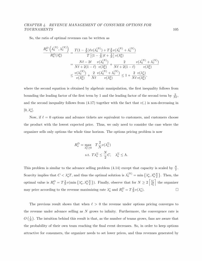
CHAPTER 4. REVENUE MANAGEMENT OF CONSUMER OPTIONS FORTOURNAMENTS 105
So, the ratio of optimal revenues can be written as
RDo
(λ
(N)a , λ
(N)o
)RDa (λ0
a)=T (1− 2
N )`v(λ(N)a ) + T 2
N v(λ(N)a + λ
(N)o )
T[(1− 2
N )`+ 2N
]v(λ0
a)
=N`− 2`
N`+ 2(1− `)v(λ
(N)a )
v(λ0a)
+2
N`+ 2(1− `)v(λ
(N)a + λ
(N)o )
v(λ0a)
≤ v(λ(N)a )
v(λ0a)
+2
N`
v(λ(N)a + λ
(N)o )
v(λ0a)
≤ 1 +2
N`
v(λ∗a)
v(λ0a),
where the second equation is obtained by algebraic manipulation, the first inequality follows from
bounding the leading factor of the first term by 1 and the leading factor of the second term by 2N` ,
and the second inequality follows from (4.17) together with the fact that v(.) is non-decreasing in
[0, λ∗a].
Now, if ` = 0 options and advance tickets are equivalent to customers, and customers choose
the product with the lowest expected price. Thus, we only need to consider the case where the
organizer sells only options the whole time horizon. The options pricing problem is now
RDo = maxλΣo ≥0
T2
Nv(λΣ
o )
s.t. TλΣo ≤
N
2C, λΣ
o ≤ Λ.
This problem is similar to the advance selling problem (4.14) except that capacity is scaled by N2 .
Scarcity implies that C < λ∗aT , and thus the optimal solution is λ(N)o = min
λ∗a, λ
0aN2
. Then, the
optimal value is RDo = T 2N v(min
λ∗a, λ
0aN2
). Finally, observe that for N ≥ 2
⌈λ∗aλ0a
⌉the organizer
may price according to the revenue maximizing rate λ∗a and RDo = T 2N v(λ∗a).
The previous result shows that when ` > 0 the revenue under options pricing converges to
the revenue under advance selling as N grows to infinity. Furthermore, the convergence rate is
O(
1N
). The intuition behind this result is that, as the number of teams grows, fans are aware that
the probability of their own team reaching the final event decreases. So, in order to keep options
attractive for consumers, the organizer needs to set lower prices, and thus revenues generated by

CHAPTER 4. REVENUE MANAGEMENT OF CONSUMER OPTIONS FORTOURNAMENTS 106
options subside. Because fans also obtain a positive surplus from attending a game without their
own team, more consumers choose to buy advance tickets as the number of teams grows. However,
when ` = 0 options and advance tickets are equivalent to customers, and they are only interested in
one outcome: their own team advancing to the final game. Because the probability of that outcome
converges to zero, the number of tickets sold converges to zero as well. This observation, combined
with the existence of the null price (or limλa→0 v(λa) = 0), causes the organizer’s revenue to
diminish to zero in all pricing schemes as the number of teams increases. Surprisingly, even though
the revenues when only advance tickets are offered and, when both advance ticket and options are
offered converge to zero, they do so at different rates. The rationale is that when the organizer
offers only options each team has up to C/2 tickets available. Hence, the capacity of the stadium is
extended, and for a suitable large N the organizer may price according to the revenue maximizer
rate λ∗a.
4.3.2 Social Efficiency
How do the introduction of options affect customers’ surplus? Options allow fans to hedge against
the risk of watching a team that it is not of their preference. As a consequence, a larger number of
seats will be taken by fans of the teams that are playing in the final. So, intuitively we expect the
introduction of options to increase the total surplus of the fans.
Recall that, from Theorem 2, options are beneficial to the organizer only if the capacity is
scarce and fans strictly prefer their own team over any other. Hence, we only need to consider the
consumer surplus under those assumptions, else the organizer has no incentive to sell options. The
following proposition shows that under these assumptions if the valuation random variable is IFR,
then options do increase consumer surplus. This result shows that offering options can benefit both
the promoter and the consumers. Furthermore, the result also shows that benefit increases for both
parties as ` decreases.
Proposition 4. Assume that the valuation random variable is strictly IFR. Then, in the symmetric
case, when the seats are scarce (C < λ∗aT ) and the fans strictly prefer their own team over any
other (` < 1), introducing options increases consumer surplus. Furthermore, both the absolute and
CHAPTER 4. REVENUE MANAGEMENT OF CONSUMER OPTIONS FORTOURNAMENTS 107
relative benefit of introducing options decreases as ` increases.
Proof: Let us begin by defining the total surplus of consumers that will buy an advance ticket
when the arrival intensity is λa,
SDa (λa) = TΛ(q + (1− q)`)Gv(
pa(λa)
q + (1− q)`
)= T (q + (1− q)`)s(λa)
where the surplus rate is defined as s(λa) = ΛGv
(Fv−1 (λa
Λ
)), and Giv(x) = E [(V − x)+] =∫∞
x F iv(v)dv the integrated tail of the valuations. Notice that the surplus rate is defined on [0,Λ].
Additionally, it is increasing, continuous, differentiable, non-negative, and bounded. The mono-
tonicity stems from the fact that Fv−1
is decreasing and Gv is non-increasing. Moreover, it satisfies
limλa→0 s(λa) = 0, and limλa→Λ = ΛEV . In contrast to the revenue rate, the maximum is reached
when the intensity is set to Λ, or equivalently the price set to zero. Not surprisingly, total consumer
surplus is maximized when the tickets are given away for free.
In the advance ticket and options pricing problem, two sources contribute to the total consumer
surplus. The first source is consumers who choose advance tickets over options. The second source
is consumers who chose options over advance tickets. Some algebra shows that the total consumer
surplus in terms of the arrival intensities, denoted by SDo (λa, λo), is
SDo (λa, λo) = T (1− q)`s(λa) + Tqs(λa + λo).
Observe that the formula for consumer surplus is similar to the organizer’s revenue with the excep-
tion that the value rate is replaced by the surplus rate.
Note that the derivative of the surplus rate w.r.t. λa is
ds
dλa(λa) =
λaΛ
1
fv
(Fv−1
(λa/Λ)) .

CHAPTER 4. REVENUE MANAGEMENT OF CONSUMER OPTIONS FORTOURNAMENTS 108
Composing the derivative with λa(c) = ΛFv(c) we get
(ds
dλa λa
)(c) =
ds
dλa
(ΛFv(c)
)=Fv(c)
f(c)=
1
h(c).
Strict IFR implies that the composite function is decreasing in c. Because λa(c) is decreasing, we
conclude that original derivative is increasing and s is strictly convex.
Now, we are position to prove that offering options increases consumer surplus. First, let
(λa, λo) be the optimal solution to the options pricing problem. Since seats are scarce, the capacity
constraint (4.13b) is binding in the optimal solution. Then λ0a = C/T = λa + qλo = (1 − q)λa +
q(λa + λo), where we have written λ0a as a convex combination of λa and λa + λo. Consider the
convex combination of the same points, denoted by λa, in which we multiply the first weight by `
and re-normalize. Hence, λa is given by
λa =(1− q)`
q + (1− q)`λa +
q
q + (1− q)`(λa + λo).
Notice that λa > λ0a. This follows from λo > 0 implying that the second point is strictly greater
than the first, and the weight of this larger point being larger in λa than in λ0a.
Finally, we have that
SDo = SDo (λa, λo) = T (1− q)`s(λa) + Tqs(λa + λo)
≥ T (q + (1− q)`)s(λa) > T (q + (1− q)`)s(λ0a) = SDa (λ0
a) = SDa ,
where the first inequality follows from the convexity of the surplus rate, the second inequality from
the fact that the surplus rate is increasing and λa > λ0a, and the last equality from λ0
a being the
optimal solution to the advance selling problem when seats are scarce. Thus, the introduction of
options increases consumer surplus. The proof for the sensitivity of options’ benefits w.r.t ` is
identical to the proof of Proposition 2 and is thus omitted.
CHAPTER 4. REVENUE MANAGEMENT OF CONSUMER OPTIONS FORTOURNAMENTS 109
4.4 Numerical Results
In this section we describe a set of randomized experiments conducted to evaluate the improvements
from offering options. The objective of these experiments is to study effect of introducing options
on the event manager’s revenue and consumer surplus, and to show that most of the results of
Section 4.3 are robust to the heterogeneity of the tournament structure. In order to tackle instances
of real-world size the analysis is based on the deterministic approximation of the problem.
The experiments were generated as follows. We assume that there were eight teams in a tourna-
ment; and similar to the FIFA World Cup, Rugby World Cup and the Superbowl, the tournament
is of dyadic form. The probability vector q was drawn from the probability simplex for the two
sets of teams in the tournament. The arrival rate λi and the love-of-the-game `i of each team i was
sampled from a uniform distribution between [0, 1]. We assume that a fan’s willingness to pay V is
uniformly distributed between [0, 4000], and that the stadium’s capacity was of C = 50, 000 seats.
To asses the impact of scarcity on our model we consider different load factors across tournaments.
The load factor is defined by lf = (TΛ)/C and measures the total demand relative to the size
of the stadium: the higher the load factor, the scarcer the tickets. Load factors were sampled
from a uniform distribution between [2, 10], and the sales horizon T was scaled to match the load
factor. We generated a total of 1000 different tournaments and used an interior point nonlinear
optimization algorithm with multiple starting points to solve the first stage of the options pricing
problem3.
We start by analyzing the benefits of introducing options by comparing the event manager’s
revenue and consumer surplus with the baseline case of offering only advance tickets. Figure
4.4a shows a histogram of the distribution of the relative improvement of offering options across
the different experiments. The average relative revenue improvement is 4.93% and its standard
deviation is 5.19%. Figure 4.4b shows a similar histogram for the relative improvement in consumer
surplus. The average relative consumer surplus improvement is 3.34% and the standard deviation
is 4.45%.
3The experiment takes about 12 hours to run in MATLAB on a PC with a 8-core Xeon processor.
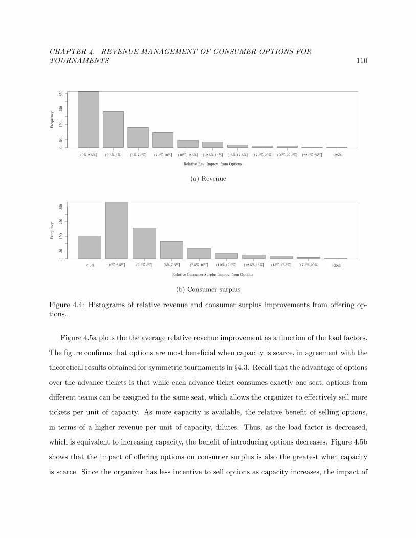
CHAPTER 4. REVENUE MANAGEMENT OF CONSUMER OPTIONS FORTOURNAMENTS 110
Relative Rev. Improv. from Options
Fre
quen
cy
050
150
250
350
(0%,2.5%] (2.5%,5%] (5%,7.5%] (7.5%,10%] (10%,12.5%] (12.5%,15%] (15%,17.5%] (17.5%,20%] (20%,22.5%] (22.5%,25%] >25%
(a) Revenue
Relative Consumer Surplus Improv. from Options
Fre
quen
cy
050
150
250
350
≤ 0% (0%,2.5%] (2.5%,5%] (5%,7.5%] (7.5%,10%] (10%,12.5%] (12.5%,15%] (15%,17.5%] (17.5%,20%] >20%
(b) Consumer surplus
Figure 4.4: Histograms of relative revenue and consumer surplus improvements from offering op-tions.
Figure 4.5a plots the the average relative revenue improvement as a function of the load factors.
The figure confirms that options are most beneficial when capacity is scarce, in agreement with the
theoretical results obtained for symmetric tournaments in §4.3. Recall that the advantage of options
over the advance tickets is that while each advance ticket consumes exactly one seat, options from
different teams can be assigned to the same seat, which allows the organizer to effectively sell more
tickets per unit of capacity. As more capacity is available, the relative benefit of selling options,
in terms of a higher revenue per unit of capacity, dilutes. Thus, as the load factor is decreased,
which is equivalent to increasing capacity, the benefit of introducing options decreases. Figure 4.5b
shows that the impact of offering options on consumer surplus is also the greatest when capacity
is scarce. Since the organizer has less incentive to sell options as capacity increases, the impact of
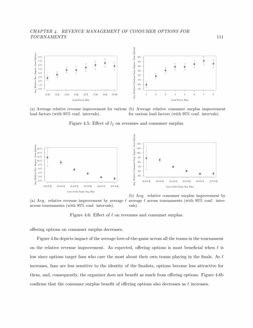
CHAPTER 4. REVENUE MANAGEMENT OF CONSUMER OPTIONS FORTOURNAMENTS 111
Load Factor Bins
Avg.
Rel
ativ
e R
ev.
Impro
v. fr
om O
pti
ons
0 %
1 %
2 %
3 %
4 %
5 %
6 %
7 %
8 %
(2,3] (3,4] (4,5] (5,6] (6,7] (7,8] (8,9] (9,10]
(a) Average relative revenue improvement for variousload factors (with 95% conf. intervals).
Load Factor Bins
Avg. R
elati
ve
Consu
mer
Surp
. Im
pro
v. fr
om
Opti
ons
−1%
0%
1%
2%
3%
4%
5%
6%
1 2 3 4 5 6 7 8
(b) Average relative consumer surplus improvementfor various load factors (with 95% conf. intervals).
Figure 4.5: Effect of lf on revenues and consumer surplus.
Love of the Game Avg. Bins
Avg.
Rel
ativ
e R
ev. Im
pro
v. fr
om O
pti
ons
0 %
2 %
4 %
6 %
8 %
10 %
12 %
14 %
16 %
(0.2,0.3] (0.3,0.4] (0.4,0.5] (0.5,0.6] (0.6,0.7] (0.7,0.8]
(a) Avg. relative revenue improvement by average `across tournaments (with 95% conf. intervals).
Love of the Game Avg. Bins
Avg.
Rel
ativ
e C
onsu
mer
Surp
. Im
pro
v.
from
Opti
ons
0%
2%
4%
6%
8%
10%
12%
14%
(0.2,0.3] (0.3,0.4] (0.4,0.5] (0.5,0.6] (0.6,0.7] (0.7,0.8]
(b) Avg. relative consumer surplus improvement byaverage ` across tournaments (with 95% conf. inter-vals).
Figure 4.6: Effect of ` on revenues and consumer surplus.
offering options on consumer surplus decreases.
Figure 4.6a depicts impact of the average love-of-the-game across all the teams in the tournament
on the relative revenue improvement. As expected, offering options is most beneficial when ` is
low since options target fans who care the most about their own teams playing in the finals. As `
increases, fans are less sensitive to the identity of the finalists, options become less attractive for
them, and, consequently, the organizer does not benefit as much from offering options. Figure 4.6b
confirms that the consumer surplus benefit of offering options also decreases as ` increases.

CHAPTER 4. REVENUE MANAGEMENT OF CONSUMER OPTIONS FORTOURNAMENTS 112
4.5 Conclusion
In this chapter we analyze consumer options that are contingent on a specific team reaching the
tournament final. Offering options, in addition to advance tickets, allows an event manager to
segment fans: advance tickets target fans with a higher willingness to pay who are less sensitive to
the outcome, whereas options target fans who receive more value from attending a game when their
favored team is in the finals. We address the problem of pricing and capacity control of such options
and advance tickets under a stochastic and price-sensitive demand model, and propose a two-stage
optimization approach to solve the problem. The first stage optimizes over the prices, while the
second optimizes the expected revenue by controlling the subset of products that is offered at each
point in time using a discrete choice revenue management model. To develop some insight, we
provide a theoretical characterization of the problem in the symmetric case, i.e., when all teams are
equal in terms of arrival rate and other characteristics. Under some mild assumptions we show that
introducing options increases both the revenue of the organizer, and the surplus of the consumers.
Numerical experiments confirm that most of these findings are robust to the heterogeneity of the
tournament structure.
One promising line of future research involves relaxing the no-resale restriction, and allowing
secondary markets and the selling of tickets after the tournament starts. In this case consumers
decide wether to buy in the primary market, or wait for the resale market where brokers speculate
on the resale price. The event manager, however, may exploit options as a mechanism to extract the
consumer’s surplus and potentially reduce the impact of the secondary market. Additionally, one
may relax the single quality seat restriction by dividing the stadium according to seat quality, and
considering instead a more sophisticated consumer choice model in which fans are offered a wider
array of choices. Lastly, dynamic pricing of options is a natural future line of research. Dynamic
pricing may provide higher revenues at the cost of substantially increased complexity.

CHAPTER 5. SMALL MODULAR INFRASTRUCTURE 113
Chapter 5
Small Modular Infrastructure
This chapter is based on the paper “Small Modular Infrastructure” which is joint work with Eric
Dahlgren, Prof. Klaus Lackner and Prof. Garrett van Ryzin.
To develop the case for small modular infrastructure, one must examine existing examples of
small-scale modular technologies, the determinants of economies of scale, the impact of manu-
facturing learning curves on capital costs and the effect of unit size on operating costs. It is also
important to account for the many flexibility and diversification advantages of small modular units.
Toward this end, in §5.1 we look at examples of small modular technology. §5.2 then provides a
theoretical analysis on how economies of unit scale and learning affect capital costs, and how unit
size affect operating costs. In §5.3 we use the U.S. electricity industry as a case study to validate
the theoretical concepts. §5.4 looks at the flexibility advantages that come with employing small
modular units, such as investment flexibility and diversification. In §5.5 we give examples of several
technologies where the trend of ever increasing size has been observed but which could benefit from
smaller unit scale. Lastly, §5.6 concludes with some general observations about how to make the
transition to “thinking small”.
CHAPTER 5. SMALL MODULAR INFRASTRUCTURE 114
5.1 Examples
Before analyzing the case for small unit scale in more depth, it is helpful to consider some examples
from the industry. Small, modular nuclear reactors, chlorine plants, and biomass gasification sys-
tems are technologies that are either already commercially available or currently under development,
and importantly, these technologies have taken advantage of small unit scale and the economies of
mass manufacturing. The specific technologies are very different, and they face different impedi-
ments to a large unit scale; regulatory hurdles for nuclear power, safety hazards for the production
and transportation of chlorine and the distributed nature of the inputs for biomass gasification.
In each case, these idiosyncratic reasons were enough to make small unit scale a feasible option.
Despite their differences, these examples hint at the common underlying potential of a radically
new strategy for building infrastructure: modularize, automate and mass produce.
5.1.1 Small modular reactors (SMRs)
Small-scale nuclear power may seem counter-intuitive, but there is growing interest in a new genera-
tion of small, modular nuclear reactors (SMRs). Unlike existing generators with an average capacity
close to 1 GWe, SMRs have capacities as small as 25 MWe (Nuclear Energy Institute, 2011; Adee
and Guizzo, 2010). Because they are small, reactors can be manufactured off-site and transported
to location semi- or fully-constructed; some are even small enough to be transported by truck. As
a result, the time required to bring a new plant on line – one of the biggest obstacles for nuclear
power – is shortened from an average of twelve to less than five years (Kadak et al., 1998; Cohen,
1990). Along with long lead times, high capital costs have been a major impediment to nuclear
power. A typical large-scale nuclear power plant requires a minimum investment of around $12
billion in capital (Wald, 2011). With SMRs, the upfront capital cost can be as low as $100 million.
Moreover, investors can easily expand a plant in the future depending on market conditions (The
Economist, 2010). Scalability of SMRs also makes nuclear power attractive for smaller projects,
thereby increasing the market for such technology. For example, SMRs can be used as “drop-in
replacements” in aging power plants since they can utilize the existing transmission capacity or

CHAPTER 5. SMALL MODULAR INFRASTRUCTURE 115
as power sources in remote applications like mining and oil and gas production where dependable
baseload power is crucial (The Economist, 2010; Hyperion Power Generation, 2011).
While SMRs can be thought of as scaled down versions of classical reactors, they also share a
common set of design characteristics that make them safer than classical reactors (Kuznetsov, 2004).
Consequently, safety and support systems are less complex. In addition, due to their modularity,
major maintenance tasks can be handled by shipping the entire reactor unit back to the factory.
These factors can reduce the on-site staff size, per unit of power output fivefold compared to
traditional nuclear power plants (Kadak et al., 1998). Another operational advantage of SMRs is
the reduced impact of maintenance down-time. Current nuclear power plants typically have one or
two reactors, so during maintenance they lose most, if not all, of their generating capacity. With
SMRs, a power plant would have 4-12 reactors, so if one reactor is taken off-line for maintenance,
the impact on total generation capacity is much less (Kadak et al., 1998).
There are numerous small modular reactors being designed around the world. Examples include
Toshiba’s 4S, Babcok & Wilcox’s mPower, Hyperion’s HPM, and Rosatom’s KLT-40. Currently,
most of the designs are being approved, and the first SMR plant is expected to be operational by
2018 (Smith, 2010). There are also plans to use SMRs in unconventional settings. For example,
Rosatom, a Russian state corporation in charge of the nuclear complex, has ordered the construction
of several floating nuclear power stations. The first, Akademik Lomosonov, was launched in 2010
and is expected to become operational by 2016 (World Nuclear News, 2012). Another example is the
small offshore reactor Flexblue developed by DCNS, a French Naval shipyard company. Commercial
production is scheduled to commence by 2016 (World Nuclear News, 2011).
Nascent SMRs provide a sense of how a radically smaller unit scale can fundamentally disrupt
an industry accustomed to massive scale. Their designs are simplified and standardized; they are
manufactured in the factory and not in the field; investment is significantly more flexible and less
risky; and their small size opens entirely new domains of applications for nuclear power. All these
are key advantages of the small modular approach to technology.

CHAPTER 5. SMALL MODULAR INFRASTRUCTURE 116
5.1.2 Small modular chlorine plants
Chlorine is widely used for the production of industrial and consumer products, disinfection and
water purification. Being highly toxic, chlorine is dangerous to store and transport. For example,
in a highly publicized train crash in 2005 in Graniteville, South Carolina, rail tank cars carrying
chlorine ruptured resulting in the death of nine people and the evacuation of thousands of residents
(Bogdanich and Drew, 2005). To avoid the costs and risks associated with chlorine storage and
transportation, companies such as GE, MIOX and AkzoNobel have designed small skid-mounted
modular chlorine plants which can be placed close to points of demand. Manufacturing these
modular plants off-site reduces on-site construction requirements, shortening the time needed to
bring a plant online. Modular design also enables efficient inspection and maintenance, reducing
operational costs. All designs are highly automated, which decreases the requirement for on-site
skilled personnel. Moreover, AkzoNobel’s design aims to completely eliminate on-site personnel
requirement by controlling the facilities remotely, thus realizing the scale benefits of traditional
chlorine plants by providing centralized monitoring and control.
Small modular chlorine plants have been around for some time. GE’s Cloromat has been in
commercial use for over 35 years and, MIOX has been producing its own line of plants since 1994
(GE Power & Water, 2011; MIOX Corporation, 2011). AkzoNobel’s solution is quite new, with the
first plant targeted to come online in 2012 (Akzo Nobel N.V., 2011; UHDENORA, 2011).
This trend of small modular chlorine plants hints at what is possible more broadly with a
strategy of small unit scale. Production is distributed and located close to points of demand,
eliminating the need for transportation. Plant designs are standardized and mass produced to
reduce capital costs. And on-site labor is minimized - or even eliminated - by utilizing advanced
sensing, automation and communications technology that enable remote control of plant operations.
The overall approach achieves many of the capital and labor savings of large unit scale yet provides
benefits, such as distributed operation, that can only be achieved with small plants.

CHAPTER 5. SMALL MODULAR INFRASTRUCTURE 117
5.1.3 Small modular biomass gasification systems
Biomass, e.g. wood and agricultural waste, is a widely available resource that can be used to
produce electricity and heat through gasification. Being abundant, biomass is a good candidate for
use in distributed electricity production and accounts for approximately 1-2% of U.S. electricity
production (EIA, 2010a).
Several companies such as AESI, Community Power Corporation(CPC) and Innovative Energy
Inc.(IEI) have commercially available designs for small modular gasification devices. These devices
convert biomass into synthesis gas to generate electricity and heat. AESI’s and CPC’s units have
capacities in the range of 50-100 kWe and IEI produces standard 1-2 MWe units (Community Power
Corporation, 2011b; AESI Inc., 2011; Innovative Energy Inc., 2011). Because of their small size,
AESI and CPC ship their systems in a small number of shipping containers which are connected
to each other on-site. This modular approach allows for easy integration and shortens the time
required to get a system operational. IEI’s system is larger, but it is also brought to the site
semi-manufactured where it is connected to existing units and infrastructure. All designs are
highly automated and CPC’s design allows its equipment to be controlled remotely from a central
location over the internet.
Like modular chlorine plants, small modular biomass gasification systems have already been
deployed in numerous projects. IEI is constructing a 5 MWe waste-to-energy power plant in Mis-
souri, and AESI has deployed its system at a pharmaceutical plant in North Carolina (Cure, 2011;
Tomich, 2010). CPC lists numerous institutions, such as Kedco, Shell Solar, Idaho Power Cor-
poration and Western Regional Biopower Energy Program, as its customers (Community Power
Corporation, 2011a).
Again, this example of small modular biomass plants illustrates a broader strategy of combining
mass manufacturing and highly automated operations to enable small unit scale plants to achieve
economies of capital and operating costs comparable to their larger brethren, while creating entirely
new benefits such as short lead times and distributed operation only achievable by small scale
technology.

CHAPTER 5. SMALL MODULAR INFRASTRUCTURE 118
5.2 A theory of unit scale
We next look at the theory on the fundamental factors that drive the choice of unit size and
how these factors are changing due to advances in technology. Our analysis considers capital
costs, operating costs and the benefits of flexibility. Collectively, the theory points to significant
advantages to radically reducing unit scale.
5.2.1 Capital costs
Given a prototype unit of known cost, one can follow two different strategies to scale up output.
One option is to create a single large unit of sufficient capacity; in effect, simply scaling up the size
of the prototype. The other option is to provide a large number of standardized units that aggregate
to produce the total desired output. Such a massively parallel production strategy is possible as
long as there is no significant cost to combining the separate outputs into a single stream.
Capital cost, regardless of strategy, is an important determinant of the economic viability of any
project. The literature on cost engineering offers empirical relations between the cost of the required
equipment and output for both strategies. In this section, we compare these costs and conclude
that, based on established empirical relationships, the cost per unit of capacity approximately scales
the same in both cases. Hence, capital cost considerations are not likely to determine the optimal
size of the production equipment. In the following, we will refer to the cost reductions achievable
in the two cases as the economies of unit scale and economies of mass production, respectively.
5.2.1.1 Economies of unit scale
A traditional method of estimating the cost k of a piece of equipment with capacity c uses a power
law:
k(c) = k(c0)
(c
c0
)α, (5.1)
where k(c0) is the cost of a reference unit of capacity c0. If the exponent is less than unity (α < 1),
the cost per unit size is decreasing, (d(k(c)/c)/dc < 0), creating an impetus for building larger units.
Numerical values for α have been estimated for a wide array of process equipment. Typically these

CHAPTER 5. SMALL MODULAR INFRASTRUCTURE 119
range from 0.6 to 0.8 (Humphreys and Katell, 1981; Jenkins, 1997; Euzen et al., 1993), hence the
so-called “0.7 rule,” or sometimes “two-thirds rule.” However, at very large sizes the structural
integrity of materials becomes an issue. Consequently, pushing the boundaries on the large end
of the spectrum has normally been accompanied by development in materials that are lighter and
stronger, as for example in the use of carbon fibers in wind turbine construction (see (Levin, 1977)).
The observed decline in cost of equipment with increasing unit size can be attributed to several
factors mentioned above. However, a frequently cited explanation for the appearance of the scaling
law in (5.1), with the exponent α ranging from 0.6 to 0.8, relies on the geometric relationship
between surface area and volume (Haldi and Whitcomb, 1967; Husan, 1997; Tribe and Alpine,
1986; van Mieghem, 2008). This explanation suggests that costs scale with the amount of material
used in the structure, which in turn is supposed to scale with surface area. Often when considering a
piece of industrial equipment like a pressure vessel, a chemical reactor or a truck bed, it is reasonable
to assume that its capacity is proportional to its useful volume. If both assumptions apply, scaling
the capacity with a factor λ results in costs scaling as λ2/3. This offers a nice explanation for the
often-observed value of α ≈ 2/3 in (5.1).
However, from the perspective of structural mechanics, this argument is flawed. In most situ-
ations, as the volume of a structure is increased, it is necessary to increase the wall thickness as
well in order to preserve structural integrity. As a result, the mass of an optimally designed unit
typically increases more rapidly than the 2/3 power of the enclosed volume. Indeed, in any situa-
tion in which the weight of the structure matters, it is usually not even possible to achieve uniform
scaling, i.e. all linear dimensions increase by the same scaling factor, λ1/3. Instead, wall thicknesses
or diameters of structural members must grow faster than the linear size of the system. Therefore,
the mass of the unit, and thereby costs, would scale faster than the capacity of the system.
In living systems, the break-down of uniform scaling can be seen by comparing a mouse to an
elephant, where the latter has disproportionately thicker legs to support its weight; the same concept
holds for industrial objects. A structure operating at its mechanical capacity (with appropriate
safety factors) cannot be uniformly scaled up. The weight of the larger structure would exceed the
limits of its structural integrity. A way around this problem is to use lighter materials, stronger

CHAPTER 5. SMALL MODULAR INFRASTRUCTURE 120
materials, or a combination of the two. Typically, advanced materials are not used at smaller scales
because they are more expensive. However, even with the most advanced materials, physics imposes
a boundary which can only be pushed so far. A detailed analysis of the scaling of solid structures
can be found in (Dahlgren and Lackner, 2012). While we do not challenge the observed empirical
relationship between cost and unit size, we submit that the conventional explanation, that the wall
area to volume ratio drives scaling behavior, is overly simplistic and under more careful analysis
proves incorrect. Instead, structural constraints tend to reduce cost advantages of larger units, and
if these constraints were to dominate, they would result in diseconomies of unit scale.
5.2.1.2 Economies of mass production
Studies of the economies of mass production date back to Wright (1936) in the context of airplane
production. Arrow (1962) provided a general analysis of the subject in which he argues that costs of
manufactured goods decline with the cumulative number produced. There have since been various
studies resulting in ample data on the cost reduction with cumulative production (see e.g. (Argote
and Epple, 1990; Ferioli and van der Zwaan, 2009; McDonald and Schrattenholzer, 2001; Tsuchiya
and Kobayashi, 2004)).
Costs decline as cumulative output increases because of specialization in the production process
and improved process and product design. For example, when organizing a production process to
manufacture a large number of identical units, one can justify high degrees of specialization in tools,
layout and job design that can dramatically reduce per-unit manufacturing costs. Also, in high-
volume manufacturing, it becomes justifiable to invest significantly in product design in order to
make parts and subsystems more integrated, easier to assemble and hence less costly to make (design
for manufacturing). The second benefit of producing in volume is learning. As a manufacturer gains
cumulative experience producing a given product via a certain process, myriad improvements in
design, materials and production methods are uncovered. Such a process of continuous improvement
can lead to significant cost reductions as production volumes increase. Conversely, cost reductions
attributed to learning can reverse themselves given extended breaks in production. This trend,
akin to a “forgetting curve”, can explain the relatively small cost reductions over time for larger
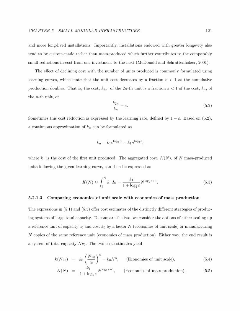
CHAPTER 5. SMALL MODULAR INFRASTRUCTURE 121
and more long-lived installations. Importantly, installations endowed with greater longevity also
tend to be custom-made rather than mass-produced which further contributes to the comparably
small reductions in cost from one investment to the next (McDonald and Schrattenholzer, 2001).
The effect of declining cost with the number of units produced is commonly formulated using
learning curves, which state that the unit cost decreases by a fraction ε < 1 as the cumulative
production doubles. That is, the cost, k2n, of the 2n-th unit is a fraction ε < 1 of the cost, kn, of
the n-th unit, or
k2n
kn= ε. (5.2)
Sometimes this cost reduction is expressed by the learning rate, defined by 1− ε. Based on (5.2),
a continuous approximation of kn can be formulated as
kn = k1εlog2 n = k1n
log2 ε,
where k1 is the cost of the first unit produced. The aggregated cost, K(N), of N mass-produced
units following the given learning curve, can then be expressed as
K(N) ≈∫ N
1kndn =
k1
1 + log2 εN log2 ε+1. (5.3)
5.2.1.3 Comparing economies of unit scale with economies of mass production
The expressions in (5.1) and (5.3) offer cost estimates of the distinctly different strategies of produc-
ing systems of large total capacity. To compare the two, we consider the options of either scaling up
a reference unit of capacity c0 and cost k0 by a factor N (economies of unit scale) or manufacturing
N copies of the same reference unit (economies of mass production). Either way, the end result is
a system of total capacity Nc0. The two cost estimates yield
k(Nc0) = k0
(Nc0
c0
)α= k0N
α, (Economies of unit scale), (5.4)
K(N) =k1
1 + log2 εN log2 ε+1, (Economies of mass production). (5.5)

CHAPTER 5. SMALL MODULAR INFRASTRUCTURE 122
A statistical analysis based on a sample of 22 different mass-production-oriented industrial sectors
found an average learning rate of 19% (Ferioli et al., 2009), which corresponds to a value of the
exponent in (5.5) of 0.7, i.e. log2 ε+ 1 = 0.7. Since typical values for the exponent α in (5.4) range
between 0.6 to 0.8 it is reasonable to conclude that log2 ε + 1 ≈ α and hence, the reductions in
production costs ensuing from economies of mass production are on par with those from economies
of unit scale.
This comparison assumes that the total installed capacity is independent of the choice of unit
size, which would be true, for example, in building a single factory. However, smaller unit sizes
frequently opens up new domains of application for a given technology, and hence increase the
overall market size. The increased volume of demand from an increased market, in turn, further
reduces cost per unit capacity. For example, as noted in §5.1.1, current sizes of nuclear reactors
make them infeasible for a wide range of applications. With the introduction of SMRs, nuclear
energy is a viable option for much smaller projects such as powering remote mining operations.
5.2.2 Operating costs
As noted previously, high conversion and labor efficiencies are traditional benefits of large unit scale
production. However, their impacts on cost have changed dramatically with advances in technology.
Given these advances, one must take a closer look at the benefits of scale and how technology can
capture these benefits without resorting to large unit scales.
5.2.2.1 Labor efficiency
When the amount of labor scales with the number of separate units employed, rather than with
individual unit size, scaling up unit sizes naturally increases labor productivity. Arguably, this has
been a common motivation in many energy and materials processing industries in the past century,
thereby driving, at least in part, the trend of ever increasing unit size. Notable examples can be
found in the electricity generation sector, see §5.3, and in the the mining industry, as detailed in
§5.5.3. However, as remarked in section 5.2.1.1, such a strategy for increasing labor productivity
will eventually run into physical barriers that are progressively harder to surmount.
CHAPTER 5. SMALL MODULAR INFRASTRUCTURE 123
An alternative strategy to reduce labor cost is to employ automation which can ultimately drive
labor cost to zero, or at least decouple it from the number of individual units employed. Naturally,
every process has its own characteristics and its amenability to automation needs to be evaluated
on a case-by-case basis. However, progress in wireless communication, GPS technology, sensor
technologies and computational processing power is fundamentally changing the economics of au-
tomation; the capabilities of these technologies are soaring while costs are plummeting, enabling
unprecedented degrees of low-cost automation. To be specific, Nordhaus (2002) reports that the av-
erage price of computing power decreased by more than 40% per year between the years 1990-2002.
The communication sector has also seen significant advances. International Telecommunication
Union (ICT) reports that the average price for a high-speed Internet connection dropped by 52%
in the world between the years 2008-2010, and Akamai reports that average global peak connec-
tion speed increased by 67% between 2010-2011 (International Telecommunication Union, 2011;
Kaufmann, 2011). The result is that automation and remote sensing and control technologies now
provide tremendous capability at very low cost.
Common instances of such automation include electronic toll collection, ATMs and electronic
check-ins for flights. In the case of ATMs and car-sharing services such as ZipCar, automation has
changed industry dynamics by making it possible to serve areas and markets that were previously
too costly. While automation does not eliminate all the benefits of increasing unit scale, given the
current state of technology, automation has often become cheaper than employing human workers,
and this reduces the benefits of large unit scale significantly.
Two other strategies to decouple labor cost from unit scale and geography are remote opera-
tion and centralized maintenance. With appropriate instrumentation and automation technologies
linked to the Internet, a central control center can monitor and operate units remotely, eliminating
the need to have on-site personnel at every location and increasing utilization of operators due
to pooling economies. As a result, labor costs become independent of the physical proximity of
the units, and there is less incentive to keep units together geographically. Similarly, small units
requiring maintenance can be shipped back to the manufacturer or to a local maintenance center
for major repairs and upgrades. Again, this eliminates the need for a local maintenance staff and

CHAPTER 5. SMALL MODULAR INFRASTRUCTURE 124
creates pooling economies in maintenance and repair. The examples of SMRs and modular chlorine
plants described in §5.1 illustrate these ideas in practice. When combined with automation tech-
nology, remote operation and centralized maintenance enable small-unit-scale technology to achieve
levels of labor cost previously obtainable only by centralization and massive unit scale.
5.2.2.2 Conversion efficiency
Conversion efficiency is the ratio of inputs to outputs, for example how much energy or raw material
is required to produce a unit of output. In some cases, the geometrical ratios of surface area to
enclosed volume, might suggest a higher conversion efficiency, such as the reduction of thermal losses
from working fluids discussed previously. In a similar way, geometry also influences the efficiency
in turbines and compressors where the main frictional losses occur along the spinning structure’s
circumference, which scales linearly with the size of the turbine, while the power output scales
proportional to the spinning structure’s area, which grows like the square of the size. Hence, the
output power grows faster with increasing size than the majority of frictional losses. Other scaling
efficiencies arise from wasted materials in batch production processes of compounds (specialty
chemicals, pharmaceuticals, cosmetics, etc.), since residue waste tends to grow like the area of a
vessel, while the output capacity grows like the vessel’s volume. So again, larger unit scale tends
to improve conversion efficiency of these processes.
While one cannot disregard these geometrical arguments for conversion efficiency due to large
unit scale, these arguments provide only a guideline and need to be evaluated on a case-by-case
basis. For example, thermal power generation, previously discussed as a case for increasing unit
size, does indeed seem to favor a larger size when considering constant operation. However, it is less
clear how significant these size-dependent conversion efficiencies are in practical operation, see §5.3,
Figure 5.2. Furthermore, a car engine operated under optimal conditions can exhibit conversion
efficiencies in the range of 30-35% which is similar to those of large single-cycle power plants (White
et al., 2006). Another such example is water desalination using reverse osmosis explained in §5.5.2.
Small-scale desalination systems intended to provide fresh water on board recreational sailboats
exhibit specific power consumption on par with modern utility-scale plants. Moreover, conversion
CHAPTER 5. SMALL MODULAR INFRASTRUCTURE 125
efficiencies are primarily important when inputs are costly, such as fossil fuels or other purchased
feed stocks. When inputs are sourced from the ambient environment, and hence effectively“free”, as
is the case for example with renewable energy technologies, the importance of efficiencies is greatly
reduced.
In summary, conversion efficiency clearly plays a role in deciding between large and small scale
unit production. However, one must take into account the variation exhibited under suboptimal
operating conditions and the cost of the input sources rather than relying simply on accepted
doctrine. Indeed, the next section illustrates this point for the U.S. electric power industry.
5.3 Case study: U.S. Electricity generating sector
In this section we analyze the size choice of the U.S. electricity generation industry and how it
affects its operating cost structure. Figure 5.1 demonstrates that electricity generation is a prime
example of the trend of building larger and larger units. (The surveyed capacity encompasses more
than 80% of U.S. total installed capacity in 2011.) The average generator size for each technology
is increasing over time as the total cumulative capacity goes up. The trend of increasing unit
sizes is especially apparent during growth phases of a specific technology. For instance, during the
primary growth phase of coal-fired generation between 1950 and 1980, the average generator size
increased from 50 MW to almost 600 MW. Once the growth stagnates in a technology, niche and
small installations are still built, explaining the apparent decrease in average unit sizes in coal and
hydro power. The history of natural gas-fired generation is complicated by “The Powerplant and
Industrial Fuel Use Act” enacted by the U.S. Congress in 1978 and later repealed in 1987. This
law effectively banned new construction of natural gas-fired power plants, explaining the slump in
average sizes during this period.
We can at least partially explain this trend of “bigger is better” by economies of unit scale
across the entire electricity generating industry. Examples of numerical values for the scale factor, α,
introduced in equation (5.1), used for engineering capital cost estimates for the various technologies
can be found in Table 5.1. Decreasing capital costs by scaling up has clearly been a benefit to the
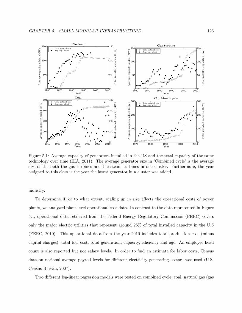
CHAPTER 5. SMALL MODULAR INFRASTRUCTURE 126
1960 1970 1980 1990 2000 20100
500
1000
1500
Averagecapacity
added
(MW
)
Year
Nuclear
0
50
100
150
Totalinstalled
capacity
(GW
)
Total installed cap.Avg. cap. added
1960 1970 1980 1990 2000 20100
50
100
150
Averagecapacity
added
(MW
)
Year
Gas turbine
0
50
100
150
Totalinstalled
capacity
(GW
)
Total installed cap.Avg. cap. added
1950 1960 1970 1980 1990 2000 20100
200
400
600
800
Averagecapacity
added
(MW
)
Year
Coal
0
100
200
300
400
Totalinstalled
capacity
(GW
)
Total installed cap.Avg. cap. added
1970 1980 1990 2000 20100
100
200
300
Averagecapacity
added
(MW
)
Year
Combined cycle
0
100
200
300
Totalinstalled
capacity
(GW
)
Total installed cap.Avg. cap. added
Figure 5.1: Average capacity of generators installed in the US and the total capacity of the sametechnology over time (EIA, 2011). The average generator size in ’Combined cycle’ is the averagesize of the both the gas turbines and the steam turbines in one cluster. Furthermore, the yearassigned to this class is the year the latest generator in a cluster was added.
industry.
To determine if, or to what extent, scaling up in size affects the operational costs of power
plants, we analyzed plant-level operational cost data. In contrast to the data represented in Figure
5.1, operational data retrieved from the Federal Energy Regulatory Commission (FERC) covers
only the major electric utilities that represent around 25% of total installed capacity in the U.S
(FERC, 2010). This operational data from the year 2010 includes total production cost (minus
capital charges), total fuel cost, total generation, capacity, efficiency and age. An employee head
count is also reported but not salary levels. In order to find an estimate for labor costs, Census
data on national average payroll levels for different electricity generating sectors was used (U.S.
Census Bureau, 2007).
Two different log-linear regression models were tested on combined cycle, coal, natural gas (gas

CHAPTER 5. SMALL MODULAR INFRASTRUCTURE 127
Technology α
Gas turbine + HRSG 0.7 (Hamelinck and Faaij, 2002)Steam turbine + steam system 0.7 (Hamelinck and Faaij, 2002)Nuclear power plant 0.619 (Locatelli and Mancini, 2010)Hydroelectric plant 0.82 (Hreinsson, 1987)
Table 5.1: Scale factors for various electricity generating technologies (HRSG – Heat recovery steamgenerator).
turbine) and nuclear generation technologies to determine if the size of a generator significantly
influences operating costs. These four technologies studied together represent more than 75% of
U.S. electricity generating capacity. The remaining two main technologies not included in this study
are hydroelectric generation and natural gas fired steam cycle plants. The former technology was
excluded since is has no fuel cost and the latter since it is an outdated technology. The total sample
size in this study represents around 270 GW of capacity, or almost 25% of total U.S. generation
capacity. Each technology sample accounts for at least 20% of installed capacity in the U.S. for
that technology.
In the first model the dependent variable is the total cost per kWh of electricity produced,
whereas the second model analyzes only the non-labor portion of the costs. In both models the
independent variables were the average generator size, capacity factor, fuel cost, efficiency and age.
A complete result of the analysis, together with a more detailed description of the data can be
found in Appendix D.
The analysis of the first model, examining total production costs, showed that increasing size
significantly decreases operating costs for nuclear and gas turbine technologies. Neither coal nor
combined cycle technologies exhibited any significant trend with respect to unit size. In the second
model where labor costs are removed, none of the technologies show any residual reduction in cost
with increasing unit size. Moreover, in this case coal even exhibits a significant increasing trend in
cost with respect to size. The difference between the two regression analysis supports the argument
presented in §5.2.2. Building larger units does, to a first approximation, decrease labor cost per
unit output produced. But unit size has no discernible effect on the remaining operating costs.
Besides labor cost, the other variable cost factor discussed in §5.2.2 possibly acting to drive
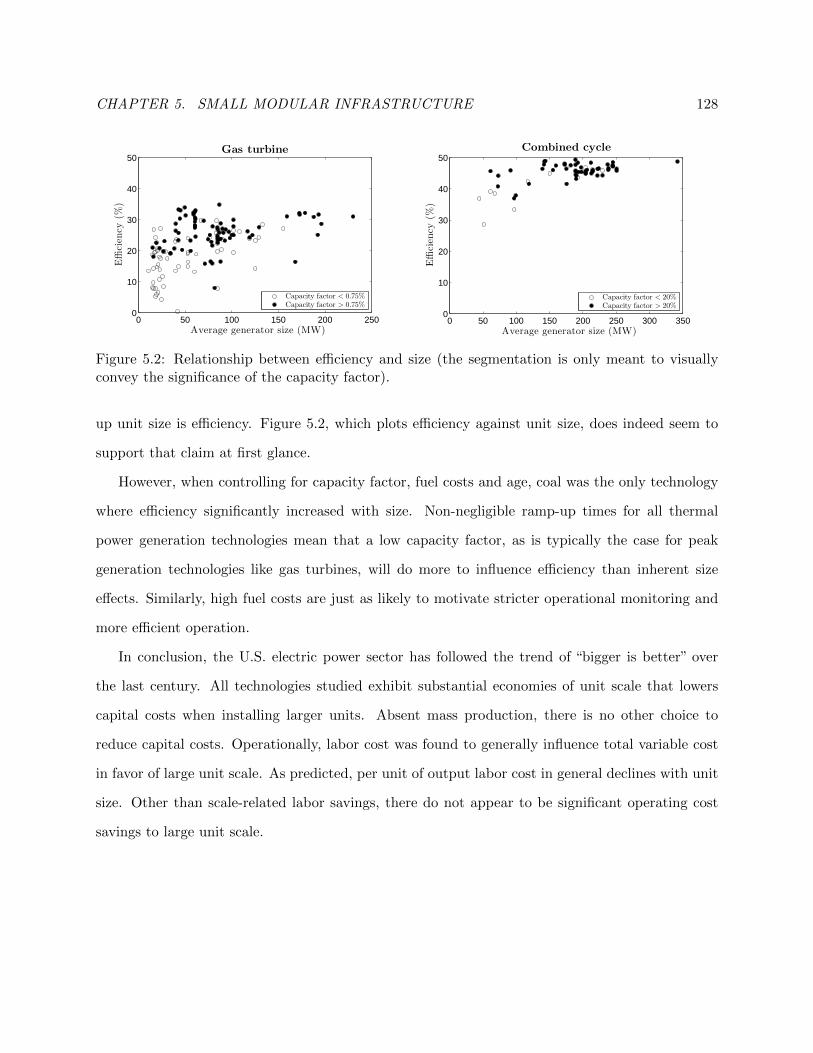
CHAPTER 5. SMALL MODULAR INFRASTRUCTURE 128
0 50 100 150 200 2500
10
20
30
40
50
Efficien
cy(%
)
Average generator size (MW)
Gas turbine
Capacity factor < 0.75%Capacity factor > 0.75%
0 50 100 150 200 250 300 3500
10
20
30
40
50
Efficien
cy(%
)
Average generator size (MW)
Combined cycle
Capacity factor < 20%Capacity factor > 20%
Figure 5.2: Relationship between efficiency and size (the segmentation is only meant to visuallyconvey the significance of the capacity factor).
up unit size is efficiency. Figure 5.2, which plots efficiency against unit size, does indeed seem to
support that claim at first glance.
However, when controlling for capacity factor, fuel costs and age, coal was the only technology
where efficiency significantly increased with size. Non-negligible ramp-up times for all thermal
power generation technologies mean that a low capacity factor, as is typically the case for peak
generation technologies like gas turbines, will do more to influence efficiency than inherent size
effects. Similarly, high fuel costs are just as likely to motivate stricter operational monitoring and
more efficient operation.
In conclusion, the U.S. electric power sector has followed the trend of “bigger is better” over
the last century. All technologies studied exhibit substantial economies of unit scale that lowers
capital costs when installing larger units. Absent mass production, there is no other choice to
reduce capital costs. Operationally, labor cost was found to generally influence total variable cost
in favor of large unit scale. As predicted, per unit of output labor cost in general declines with unit
size. Other than scale-related labor savings, there do not appear to be significant operating cost
savings to large unit scale.

CHAPTER 5. SMALL MODULAR INFRASTRUCTURE 129
5.4 Flexibility and diversification
There are inherent flexibility and diversification benefits that can be attained only at a smaller unit
scale. A careful examination of these benefits shows that they can be highly significant and may
easily tip the scale in favor of small unit scale. Changes in cost functions, scaling relationships or
scale-dependent flexibility and diversification benefits – like those driven by advances in technology
– can lead to a “tipping point,” at which the optimal scale switches discontinuously from large to
small. The evolution of super computer technology discussed above illustrates a powerful real-world
example of this tipping point phenomenon. The ‘supercomputer market crash’ of the mid 1990s
occurred when mass-produced CPUs from the expanding personal computer industry, somewhat
suddenly, reached a tipping point where it became less costly to achieve high computing capacity
using large numbers of small-scale CPUs in parallel and demand for traditional super computers
collapsed. This historical example underscores the point that shifts in optimal unit scale due
to technological advances can occur rather suddenly and result in dramatic disruptions of entire
industries.
5.4.1 Locational flexibility
Unlike large-unit-scale technologies, small unit scale offers the option of either centralization or
decentralization. Multiple units can be aggregated at a single location to achieve economies of
centralization in, for example, pooling the risk of demand variation. Alternatively, units can be
distributed closer to sources of supply or points of demand and thereby reduce transport or trans-
mission costs of either in- or out-bound goods.
An example that demonstrates the benefits of decentralization is distributed electricity gener-
ation as noted by Lovins et al. (2002). According to International Energy Agency (2002), on-site
generation could result in 30% cost savings in transmission and distribution, which together ac-
count for above 40% of the cost of electricity for residential customers. Furthermore, distributed
generation allows for the combined generation of heat and electricity which can result in energy
savings from 10% to 30%, depending on the type and size of co-generation units (Pepermans et al.,

CHAPTER 5. SMALL MODULAR INFRASTRUCTURE 130
2005).
Decentralization also has safety and security implications. For example, while small nuclear
reactors (SMRs) may increase the domain of applications for nuclear energy, dispersed nuclear
generation offers a greater number of targets for individuals with disruptive motives. Another
concern is nuclear proliferation. With widespread adoption of nuclear technology, it becomes more
difficult to monitor nuclear fuel to ensure proper handling and secure distribution. Yet these
security risks can be managed by other means. For example, most SMRs are designed for off-
site refueling, which reduces the accessibility of the core by unauthorized personnel. In other
cases, decentralization can have the potential of improving safety and increasing security. Chlorine
production is a clear example where both storage and transportation carries significant safety risks
due to the toxicity of the product. Decentralization enables the production of chlorine close to points
of demand thus reducing the need to store and transport this hazardous substance. This results
in a substantial decrease in the safety risks associated with the use of chlorine. More generally, by
its sheer nature, a smaller scale of any technology reduces the local impact of possible catastrophic
failure.
5.4.2 Investment flexibility
Unit scale affects the flexibility of an investment in several important ways. First, small-scale units
can be used in multiples to better match the output requirements of a given project thus avoiding
either capacity shortages or excess capital investment. Second, small units can be deployed more
flexibly over time. They can be installed sequentially as uncertain demand evolves, avoiding excess
investment in the early life of a project or investment errors later in the project life cycle. Also,
mass-produced, standardized units can be built to stock and deployed more quickly than custom-
built, large-scale units, reducing the lag between investment and revenue generation. Finally, while
lifetimes of custom-built infrastructural investments tend to be very long, this need not be true for
small-scale technologies. A shorter investment cycle for small-scale technologies would allow for
disengagement if market conditions worsen without forsaking large sunk costs.
A full-fledged practical evaluation of these benefits would require detailed stochastic models

CHAPTER 5. SMALL MODULAR INFRASTRUCTURE 131
of the underlying variables, and a rigorous real option valuation. Such a valuation is made in
(Dahlgren and Leung, 2013), where the value of consecutive investments, as a function of lifetime
and lead-time, is treated as an optimal multiple stopping problem. The main finding in that study is
that increasing lifetime does not greatly increase the value of an investment scenario where multiple
consecutive investments can be made. We will here consider a couple of simple models that illustrate
the advantages of shorter lead-time and of modularity individually. These two models are adapted
from (Hoff, 1997).
5.4.2.1 Investment advantages of modularity
Being able to make investments in small increments over time provides significant economic advan-
tages. The concept is best illustrated by an example: consider a firm, such as an electric utility,
planning the future expansion of a plant to satisfy increasing demand. The firm has to satisfy all
demand and has two options for investment: modular and non-modular. The modular investment
involves increasing the capacity in increments of x and the non-modular investment involves a
one-shot investment of nx units, where n > 0. For simplicity we assume that n is an integer.
The current capacity matches the demand, and demand each year either increases by x with
probability p or stays the same with probability 1− p. The lead-time for both types of investments
is zero and the total additional capacity to be installed is nx. With the first increase in demand, the
firm can either choose to make a one-time capacity expansion of nx units or increase the capacity
in increments of x every time the demand increases, for a total of n times.
The cost of a big (non-modular) and a small (modular) investment for each increment is denoted
by Kbig and Ksmall, respectively. With a constant discount rate, r, the expected discounted cost of
the non-modular investment (occurring the first time demand increases from current level) is
Ibig =∞∑k=0
(1− p)kpKbig
(1 + r)k= Kbig
p(1 + r)
r + p.
For the modular investment scenario, we denote by Ii the expected discounted cost of the i-th
investment. This investment occurs at the end of the k-th year (k > i− 1) when demand rises for
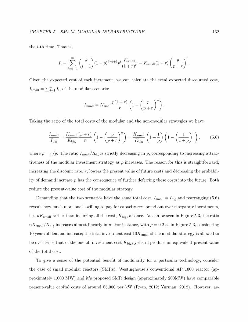
CHAPTER 5. SMALL MODULAR INFRASTRUCTURE 132
the i-th time. That is,
Ii =∞∑
k=i−1
(k
i− 1
)(1− p)k−i+1pi
Ksmall
(1 + r)k= Ksmall(1 + r)
(p
p+ r
)i.
Given the expected cost of each increment, we can calculate the total expected discounted cost,
Ismall =∑n
i=1 Ii, of the modular scenario:
Ismall = Ksmallp(1 + r)
r
(1−
(p
p+ r
)n).
Taking the ratio of the total costs of the modular and the non-modular strategies we have
Ismall
Ibig=Ksmall
Kbig
(p+ r)
r
(1−
(p
p+ r
)n)=Ksmall
Kbig
(1 +
1
ρ
)(1−
(1
1 + ρ
)n), (5.6)
where ρ = r/p. The ratio Ismall/Ibig is strictly decreasing in ρ, corresponding to increasing attrac-
tiveness of the modular investment strategy as ρ increases. The reason for this is straightforward;
increasing the discount rate, r, lowers the present value of future costs and decreasing the probabil-
ity of demand increase p has the consequence of further deferring these costs into the future. Both
reduce the present-value cost of the modular strategy.
Demanding that the two scenarios have the same total cost, Ismall = Ibig and rearranging (5.6)
reveals how much more one is willing to pay for capacity nx spread out over n separate investments,
i.e. nKsmall rather than incurring all the cost, Kbig, at once. As can be seen in Figure 5.3, the ratio
nKsmall/Kbig increases almost linearly in n. For instance, with ρ = 0.2 as in Figure 5.3, considering
10 years of demand increase; the total investment cost 10Ksmall of the modular strategy is allowed to
be over twice that of the one-off investment cost Kbig; yet still produce an equivalent present-value
of the total cost.
To give a sense of the potential benefit of modularity for a particular technology, consider
the case of small modular reactors (SMRs); Westinghouse’s conventional AP 1000 reactor (ap-
proximately 1,000 MW) and it’s proposed SMR design (approximately 200MW) have comparable
present-value capital costs of around $5,000 per kW (Ryan, 2012; Yurman, 2012). However, as-
CHAPTER 5. SMALL MODULAR INFRASTRUCTURE 133
2 4 6 8 100
0.5
1
1.5
2
2.5
3
Cost
ratio(nK
small/K
big)
Number of modular increments (n)
ρ = 0.1ρ = 0.2ρ = 0.3
Figure 5.3: The ratio nKsmall/Kbig evaluated at different n with equal total cost Ismall = Ibig andwith ρ = r/p = 0.1, 0.2, 0.3.
suming a discount rate of 5% (r = 5%) and that the probability that demand grows by 200MW in
a given year is 20% (p = 20%), the above model shows that the expected discounted total capital
cost of the SMR plant is 30-35% lower than the corresponding conventional plant.
5.4.2.2 Investment advantages of shorter lead-time
Mass-produced modular technology that is manufactured to stock can significantly reduce the lead-
time to deploy a new investment. We next examine how shorter lead-times can be beneficial in terms
of total investment costs, again via a simple example. Similar to the previous section, assume a firm
is planning the future expansion of a plant that has to satisfy increasing but uncertain demand. As
above, the demand increases by x with probability p or it stays the same with probability 1 − p.
Let T denote the minimum number of years until the current excess capacity runs out; thus, the
current excess capacity is Tx.
The firm has two options for investment. It can either invest in an expansion project with a
long lead-time Ll or a short lead-time Ls. To compare these two investment options, we assume
that T ≥ Ll > Ls. Let Kl and Ks denote the costs of expansions with long and short lead-times
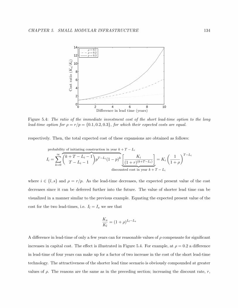
CHAPTER 5. SMALL MODULAR INFRASTRUCTURE 134
0 2 4 6 8 100
2
4
6
8
10
12
14
Cost
ratio(K
s/K
l)
Difference in lead time (years)
ρ = 0.1ρ = 0.2ρ = 0.3
Figure 5.4: The ratio of the immediate investment cost of the short lead-time option to the longlead-time option for ρ = r/p = 0.1, 0.2, 0.3, for which their expected costs are equal.
respectively. Then, the total expected cost of these expansions are obtained as follows:
Ii =∞∑k=0
probability of initiating construction in year k + T − Li︷ ︸︸ ︷(k + T − Li − 1
T − Li − 1
)pT−Li(1− p)k
[Ki
(1 + r)(k+T−Li)
]︸ ︷︷ ︸
discounted cost in year k + T − Li
= Ki
(1
1 + ρ
)T−Li
where i ∈ l, s and ρ = r/p. As the lead-time decreases, the expected present value of the cost
decreases since it can be deferred further into the future. The value of shorter lead time can be
visualized in a manner similar to the previous example. Equating the expected present value of the
cost for the two lead-times, i.e. Il = Is we see that
Ks
Kl= (1 + ρ)Ll−Ls
A difference in lead-time of only a few years can for reasonable values of ρ compensate for significant
increases in capital cost. The effect is illustrated in Figure 5.4. For example, at ρ = 0.2 a difference
in lead-time of four years can make up for a factor of two increase in the cost of the short lead-time
technology. The attractiveness of the shorter lead time scenario is obviously compounded at greater
values of ρ. The reasons are the same as in the preceding section; increasing the discount rate, r,

CHAPTER 5. SMALL MODULAR INFRASTRUCTURE 135
lowers the present value of future costs and decreasing the probability p of a demand increase has
the consequence of further deferring these costs in the future.
As previously discussed, SMRs are expected to have much shorter lead-times compared to
conventional nuclear reactors. By utilizing a methodology similar to the one in the previous section,
we can demonstrate that this can lead to significant potential cost savings. Assuming the parameters
stay the same, i.e. p = 20% and r = 5%, if the lead-time for construction decreases by 3 years, this
can lead to potential cost savings of 45-50%.
5.4.3 Operating flexibility
Small unit scale provides increased flexibility in terms of deploying partial capacity since it is
possible to selectively run varying numbers of smaller units in order to achieve a targeted level of
total output. Facilities consisting of a single large unit often have to be operated in an effectively
binary, “on-off” mode, producing either nothing or at maximum capacity. A coal-fired power plant,
for example, has a limited range of outputs for which it can operate efficiently. As a consequence,
these plants are limited to providing steady, base-load power and cannot effectively serve variable
peak-load demands or efficiently slow down to avoid waste during period of low demand.
To illustrate this idea, we rely on a model of a plant consisting of multiple units operated in an
on-off fashion with total capacity C. The plant has to satisfy a random demand D. Let n denote
the number of units in the plant, so Cu = C/n denotes the unit capacity of the equipment in the
plant. The excess operational capacity, XC , can be written as
XC = kCu −D, where k =
⌈D
Cu
⌉.
The expected excess operational capacity, E[XC ] is
E[XC ] = CuE[k]− E[D] = Cu
n∑k=1
kP [(k − 1)Cu < D ≤ kCu]− µ,
where µ is the mean demand.
Figure 5.5 depicts the average excess operational capacity for different unit capacities Cu using
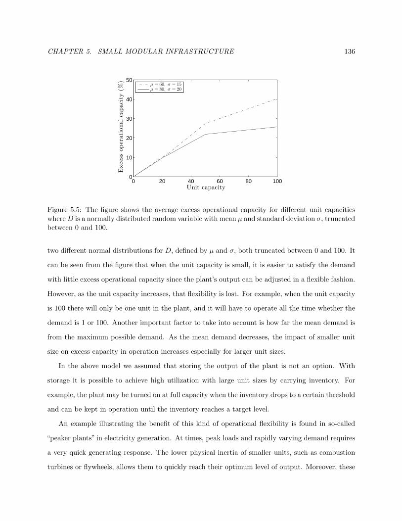
CHAPTER 5. SMALL MODULAR INFRASTRUCTURE 136
0 20 40 60 80 1000
10
20
30
40
50
Excess
operationalcapacity
(%)
Unit capacity
µ = 60, σ = 15µ = 80, σ = 20
Figure 5.5: The figure shows the average excess operational capacity for different unit capacitieswhereD is a normally distributed random variable with mean µ and standard deviation σ, truncatedbetween 0 and 100.
two different normal distributions for D, defined by µ and σ, both truncated between 0 and 100. It
can be seen from the figure that when the unit capacity is small, it is easier to satisfy the demand
with little excess operational capacity since the plant’s output can be adjusted in a flexible fashion.
However, as the unit capacity increases, that flexibility is lost. For example, when the unit capacity
is 100 there will only be one unit in the plant, and it will have to operate all the time whether the
demand is 1 or 100. Another important factor to take into account is how far the mean demand is
from the maximum possible demand. As the mean demand decreases, the impact of smaller unit
size on excess capacity in operation increases especially for larger unit sizes.
In the above model we assumed that storing the output of the plant is not an option. With
storage it is possible to achieve high utilization with large unit sizes by carrying inventory. For
example, the plant may be turned on at full capacity when the inventory drops to a certain threshold
and can be kept in operation until the inventory reaches a target level.
An example illustrating the benefit of this kind of operational flexibility is found in so-called
“peaker plants” in electricity generation. At times, peak loads and rapidly varying demand requires
a very quick generating response. The lower physical inertia of smaller units, such as combustion
turbines or flywheels, allows them to quickly reach their optimum level of output. Moreover, these

CHAPTER 5. SMALL MODULAR INFRASTRUCTURE 137
small scale generators are typically deployed in multiples, which are activated in varying numbers
to match peak load demands. The flexibility of these small generators combined with the high rates
paid for peak generation mean they can be operated profitably at very low utilizations.
5.4.4 Diversification
Small unit scale also provides significant diversification benefits. By exploiting statistical inde-
pendence of many small operating units rather than relying on a few large operating units, it is
possible reduce unit reliability yet raise overall system reliability. If all output stems from one
single large unit, a single failure can reduce output to zero, which makes it necessary to incur the
costs of substantial redundancies. If, however, the same total output is provided by 10,000 units
that are easily replaced, the impetus for built-in redundancies in any given unit are diminished.
This reduced need for high unit-level reliability can both reduce capital costs and improve service
reliability.
We illustrate this concept with the following simple example. Suppose a utility is to provide an
output capacity D, available with a probability R in a given time period (1−R is the probability
of failure). We assume that a single unit, with capacity Cu, can either be fully functioning with
probability p < R in a given time period or not at all. As a result, the utility will need redundancy
to make up for the missing reliability. So, the utility has to decide on the minimum number of units
to install, n∗, to ensure that the aggregate available capacity C(n) = nCu exceeds demand D with
a probability of at least R. With the assumed independence of the individual units this problem
can be formulated as
n∗ = min
n ≥
⌈D
Cu
⌉∣∣∣∣P (C(n) ≥ D) ≥ R,
where P (C(n) ≥ D) =n∑
s=⌈
DCu
⌉(n
s
)ps(1− p)(n−s).
For different R and Cu, Figure 5.6 shows the total capacity the utility has to invest in when D = 100
and p = 0.9. The figure shows that as the size of the individual units increase, the excess capacity
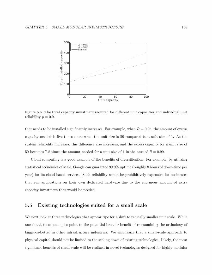
CHAPTER 5. SMALL MODULAR INFRASTRUCTURE 138
0 20 40 60 80 1000
100
200
300
400
500
Totalinstalled
capacity
Unit capacity
R = 99%R = 95%Demand
Figure 5.6: The total capacity investment required for different unit capacities and individual unitreliability p = 0.9.
that needs to be installed significantly increases. For example, when R = 0.95, the amount of excess
capacity needed is five times more when the unit size is 50 compared to a unit size of 1. As the
system reliability increases, this difference also increases, and the excess capacity for a unit size of
50 becomes 7-8 times the amount needed for a unit size of 1 in the case of R = 0.99.
Cloud computing is a good example of the benefits of diversification. For example, by utilizing
statistical economies of scale, Google can guarantee 99.9% uptime (roughly 8 hours of down-time per
year) for its cloud-based services. Such reliability would be prohibitively expensive for businesses
that run applications on their own dedicated hardware due to the enormous amount of extra
capacity investment that would be needed.
5.5 Existing technologies suited for a small scale
We next look at three technologies that appear ripe for a shift to radically smaller unit scale. While
anecdotal, these examples point to the potential broader benefit of re-examining the orthodoxy of
bigger-is-better in other infrastructure industries. We emphasize that a small-scale approach to
physical capital should not be limited to the scaling down of existing technologies. Likely, the most
significant benefits of small scale will be realized in novel technologies designed for highly modular

CHAPTER 5. SMALL MODULAR INFRASTRUCTURE 139
implementation. However, the sample technologies below exhibit either physical or economical
features (or both) in their current incarnation that strongly support a smaller scale.
5.5.1 Ammonia synthesis
Except for minor alterations to the catalyst, ammonia synthesis looks very much the same through-
out the $50 billion dollar industry of today (Erisman et al., 2008; FERTECON, 2012) as it did dur-
ing the early days of commercial implementation. One feature, however, has dramatically changed:
unit size. The first commercial plant had a capacity of 30 metric tons per day (MTPD) (Jennings,
1991), which should be compared to the currently planned facility in Collie, Australia with a nom-
inal capacity of 3,500 MTPD (Haldor Topsoe, 2009). An increase in unit capacity by two orders of
magnitudes epitomizes the aforementioned trend in unit size.
As with most catalytic processes, ammonia synthesis requires careful control of temperatures
throughout the reactor in order to maintain favorable reaction conditions. Maintaining such control
requires sophisticated internal heat exchangers, which add cost. Additionally, dealing with explosive
gases at elevated pressures exacerbates the consequences of a critical failure at larger reactor sizes.
Assuming sufficient capabilities of automation, a decrease in individual reactor size could po-
tentially reduce overall costs. First, decreasing unit size to the point that no internal heat sinks are
necessary would reduce the complexity of the individual reactor. Additionally, as explained in §5.2,
the total amount of material used will, to a first approximation, remain constant or decrease when
deploying multiple smaller units with the same aggregate capacity of a typical ammonia synthesis
reactor. Furthermore, an array of parallel smaller units would substantially mitigate the impact of
catastrophic failure of a single reactor. Also, catalytic processes, including the synthesis of ammo-
nia, all suffer from catalyst deactivation. In a monolithic setting, regenerating or replacing catalysts
requires a complete albeit temporary shutdown of the reactor. Referring to the operational flexi-
bility arguments, a more modular plant consisting of parallel units would be less exposed to such
complete but unavoidable outages. Instead of bringing the entire output to a standstill, individual
units could be swapped out and repaired off-line. These factors all point to potential cost savings
with a modular infrastructure approach.

CHAPTER 5. SMALL MODULAR INFRASTRUCTURE 140
Finally, it is worth mentioning that the main use of ammonia is in fertilizers. Serving mainly
the agriculture industry, the demand for this end-product is extremely distributed. The case for
distributed, and hence small-scale operation is further strengthened by the fact that all the inputs
necessary for the process are found in the ambient environment.
5.5.2 Water desalination
One of the main engineering challenges of the coming century is to create large, stable and affordable
supplies of fresh water from the earth’s largest water reservoir, the oceans (National Academy of
Engineering, 2012). Among the various desalination technologies available for this purpose, reverse
osmosis (RO) has seen the largest growth in recent years and represents almost half of the $20 billion
desalination market today (Greenlee et al., 2009; Fritzmann et al., 2007; Elimelech and Phillip,
2011). Some regions, notably the Middle East, parts of Australia and several island communities,
have come to rely on reverse osmosis desalination as a base load source of fresh water.
Defining a unit scale in RO operations is less straightforward than in the previous examples
because the membranes are currently manufactured and assembled in small units called modules.
Regardless, the core process of separation in a modern RO-plant encompasses three components:
a high-pressure pumping system, membrane modules housed in parallel pressure vessels, and an
energy recovery system. One of the most modern and efficient RO desalination plants in the world
is the Ashkelon plant in Israel with a capacity of 330,000 cubic meters of fresh water per day
(Sauvet-Goichon, 2007). With eight high-pressure pumps, the 40,000 cubic meters of fresh water
per day and per pumping system can serve as a benchmark for unit size in current RO desalination.
Almost half the cost of desalinated seawater through RO can be attributed to energy. Of
the remaining cost components, capital costs dominate, leaving only a minor fraction to other
variable costs (Wittholz et al., 2008). With such a cost structure, the specific energy requirement
(energy required per unit output) serves as a decent indicator of the total price of a given RO
desalination operation. Conventional wisdom would suggest that to increase the physical efficiency
of a process like RO, and hence lower the specific energy consumption, the strategy would be to
scale up unit size. Indeed, the aforementioned plant in Ashkelon is not only one of the largest
CHAPTER 5. SMALL MODULAR INFRASTRUCTURE 141
plants in the world but also one of the most efficient with electricity requirements of 3-4 kWh/m3
of produced water (Sauvet-Goichon, 2007). The notion that increased energy efficiency in RO has to
be accompanied by increased unit size is, however, contradicted by examining desalination systems
found on recreational boats. With a capacity of little more than one cubic meter per day, these
small, modular systems consume only 3.8 kWh/m3 (Spectra Watermakers, 2012), which is on par
with the utility-sized operation. While based on the exact same technology, the tight on-board
space constraints have resulted in process designs that have similar levels of energy consumption
but with smaller footprints. This indicates that a truly modular design in RO desalination could
lead to additional future cost savings as production of small units is scaled up to match large scale
demand.
5.5.3 Mining
The value of U.S. domestic production of raw materials from mining was estimated at $64 billion
dollars in 2010 (USGS, 2011). Including further downstream processing, the raw materials sector
accounts for a substantial part of GDP and is the foundation of industrial economies. While
mining operations differ substantially for different minerals in varying geologic formations, the task
of hauling ore from the point of excavation to the initial processing site is worth examining from
the perspective of unit scale. We focus here on operations in open pit, or surface mining, but the
concepts apply more broadly to other mining operations.
The cost of one mining truck driver in remote areas of Australia amounts to $150,000 per year
(quoted in Australian $, which has an exchange rate of roughly 1:1), of which more than $36,000
goes to auxiliary support such as transportation, accommodation and food (Bellamy and Pravica,
2011). Operating in three shifts, this translates into $450,000 per year per truck in labor costs.
While truck prices are hard to ascertain exactly, assuming that the investment required is on the
order of $5 million, the capital charges at 10% interest are almost on par with labor costs. Hence,
labor productivity is a key metric in evaluating mining operations. The most natural way to
increase profitability of a given mine has been to scale up the size of individual process equipment
such as loaders and haulers. Indeed, the size of the largest available haulers has increased by a
CHAPTER 5. SMALL MODULAR INFRASTRUCTURE 142
factor ten over the past 50 years. A general consequence of this trend is that smaller mines, which
preclude the use of larger equipment, become less profitable, and hence mining operations tend to
be more concentrated on large mines (Bozorgebrahimi et al., 2003; Bartos, 2007). It seems however
that this trend has stagnated recently for several reasons. For instance, auxiliary civil works,
e.g. roads and bridges, to accommodate larger trucks going in and out of a mine become more
costly. Moreover, larger equipment diminishes the possibility of selective mining techniques, thus
resulting in the transportation of lower grade ores for further processing. The complexity of larger
machinery also increases markedly at the largest end of the spectrum and hence requires additional
training of operators and repair crews as well as larger (and more expensive) maintenance facilities
(Bozorgebrahimi et al., 2003).
Even though tests have been performed recently on operating retro-fitted autonomous mining
trucks in Australian mines, such technology has not yet caught on (Bellamy and Pravica, 2011).
With non-stationary and interacting robotic systems making progress by the day, as manifested by
Google’s autonomous car (Folsom, 2011) and ‘Junior’, the driverless vehicle developed by Volkswa-
gen and Stanford through DARPA (Stanek et al., 2010), it is only a matter of time before such
technology becomes viable in isolated areas such as a mine. There is little reason why automa-
tion should proceed with the ultra-large-size equipment of today and not with much smaller units,
perhaps in the 1-10 ton class. In addition to the flexibility arguments raised in previous examples
favoring small unit size, smaller automated units can make smaller mines economical alongside
large ones, thus increasing the total resource base.
5.6 Conclusion: Learning to “think small”
When choosing from a palette of available technologies, the ultimate decision has historically been
predicated on a positive response to the question: Does the technology “scale up?” Yet as we have
argued here, our increased ability to automate and control processes without the presence of either
the human hand or mind, the capability of mass production to drastically reduce capital costs, and
a more enlightened view of the flexibility benefits of small unit scale, cast significant doubt on the

CHAPTER 5. SMALL MODULAR INFRASTRUCTURE 143
validity of the bigger-is-better mantra. As we have argued, scaling up in numbers – rather than in
unit size – can provide many of the same benefits of large unit scale and offers entirely new benefits
that can only be achieved with small unit scale. Consequently, the fundamental decision processes
surrounding the choice of technologies and their implementation need to be revisited.
Doing so, however, requires an entirely new mind set. Educators, engineers, business leaders,
financiers, standards bodies, regulators – the entire industrial ecosystem – must learn to “think
small.” In order to reap the benefits of small unit scale and achieve the needed paradigm shift,
institutional biases towards large-scale must be purged and replaced by an ability to think small.
Engineers, for one, need revised training and new conceptual tools. In today’s engineering
schools, students are instilled with the notion that unit scale-up is a precondition for the viability
of most technologies. So consequently, they focus on designing for scale economy. Instead, they
must learn how to design small – design for granularity as it were. Small modular technologies
designed to function in massively parallel configurations should not look like miniature versions of
behemoth industrial plants; they require their own distinct approach to design – one that emphasizes
off-loading control functions to central controllers, simplifies functionality to minimize the need for
ongoing control and maintenance, and reduces part counts by creating more integrated components.
Engineering small requires designs that aim to leverage the economies of mass production and
exploit the power of automation and sensors to eliminate the need for human labor. Only by
applying such design principles can the full benefits of small unit size be realized. Engineers must
also be exposed to examples of designs that are optimized for granularity, so they can develop an
instinct for how it is done.
Business leaders and financiers must likewise revise their approaches to project evaluation.
Long-standing net present value (NPV) evaluations based on simplistic pro-forma projections of
factors such as demand, cost, price, unit reliability and so on, must be replaced by the use of more
sophisticated models (of the sort illustrated in this chapter) that accurately account for the many
inherent flexibility and option-value benefits of small unit scale. Only then will their decisions be
driven by the true economic costs and benefits of unit scale.
Lastly, a mass market for small unit scale technology will not flourish unless industry leaders

CHAPTER 5. SMALL MODULAR INFRASTRUCTURE 144
recognize the potential of thinking small and create the necessary standards and common interfaces
needed to open their markets to small modular technology. Indeed, one of the reasons behind the
astonishing developments of the computer industry in the past century was the abandonment of
the mentality that every component had to be manufactured in-house. Opening up the black box
that was the computer to outside parties allowed firms to focus on fewer parts and also forced the
industry to adopt standards, resulting in the “plug-and-play” environment that eventually made
the PC possible and so dramatically successful. In addition, down-sizing, standardizing and then
proliferating technologies to a larger domain of applications further reduces costs by increasing the
aggregate market size for each technology. It also increases the likelihood of applications not yet
thought of; after all, the early pioneers of the computing industry could hardly have anticipated
the multitude of applications that permeate virtually every part of our society today, like smart
phones and video games.
These changes in mindset and industry norms will take time to develop; massively parallel
plants will not suddenly appear overnight. Indeed, there is considerable inertia in most industries
that may impede the transition to thinking small for many years to come. One explanation for this
inertia is known as the “lock-in effect” in the economics literature. As in the case of the QWERTY
keyboard, once a technology establishes dominance early on, a later superior technology may not
be able to gain market share (David, 1985). In his seminal work, Arthur (1989) shows that this
kind of a behavior is observed in industries with increasing returns to learning, as is the case with
large-scale infrastructure. But two factors offer hope that this lock-in can be overcome. For one, as
demonstrated in the preceding sections, once the flexibility and diversification benefits of small-scale
technology are recognized, these may tip the scales toward adoption. Secondly, niche applications
of small-scale technologies in areas where larger scales are infeasible or too costly may allow firms
to accumulate the necessary experience to compete with large-scale technologies in conventional
markets, as was the case with microcomputers. Once this transition happens and small scale
thinking takes root, it has the potential to radically disrupt entire industries. Like the behemoth
reptiles of the Cretaceous period, firms caught on the wrong side of such a meteoric transition will
likely suffer.

CHAPTER 5. SMALL MODULAR INFRASTRUCTURE 145
Yet despite the great promise of thinking small, we are not arguing that small-scale technology is
a panacea. Indeed, some enterprises adopting a small-scale strategy have had spectacular failures.
Even though the reasons behind its failure are disputed, one example is the geothermal energy
provider Raser Technologies that sought bankruptcy protection in 2011 (Madhani, 2011; MacFall
and Engleston, 2011; Oberbeck, 2011). And, there will always be a role for large unit scale; massive
rivers require massive hydroelectric dams, after all. Still, the concept that every industrial process
with large aggregate output requires large unit scale technology to match is fundamentally flawed
and inherently limiting. We will all benefit from a more enlightened world in which the ability to
“scale up” does not dictate our choice of technology.

BIBLIOGRAPHY 146
Bibliography
S. Adee and E. Guizzo. Nuclear redux. IEEE Spectrum, 47:25–32, 2010.
AESI Inc. Proven biomass gasification solutions by aesi. http://www.aesintl.net/solutions/
proven-biomass-gasification-solutions-by-aesi, 2011. Accessed on 2011.10.21.
P. Afeche. Incentive-compatible revenue management in queueing systems: Capacity and optimal
strategic delay. Technical report, University of Toronto, 2010.
Akzo Nobel N.V. Remote controlled chlorine production. http://www.akzonobel.com/ic/
products/remote_controlled_chlorine_production/, 2011. Accessed on 2011.10.19.
L. Argote and D. Epple. Learning Curves in Manufacturing. Science, 247(4945):920–924, 1990.
K.J. Arrow. The economic implications of learning by doing. The Review of Economic Studies,
29(3):155–173, 1962.
W.B. Arthur. Competing technologies, increasing returns, and lock-in by historical events. The
Economic Journal, 99(394):pp. 116–131, 1989.
T. Aven. Upper (lower) bounds on the mean of the maximum (minimum) of a number of random
variables. Journal of Applied Probability, 22(3):723–728, 1985.
Yossi Aviv and Awi Federgruen. The value iteration method for countable state markov decision
processes. Operations research letters, 24(5):223–234, 1999.
G. Barlow. Yield Management Strategies for the Service Industries, chapter Capacity Management
in the Football Industry, pages 303–314. Continuum, New York, NY, 2000.
BIBLIOGRAPHY 147
Paul J. Bartos. Is mining a high-tech industry? Investigations into innovation and productivity
advance. Resources Policy, 32(4):149 – 158, 2007.
Hendrik Baumann and Werner Sandmann. Numerical solution of level dependent quasi-birth-and-
death processes. Procedia Computer Science, 1(1):1561–1569, 2010.
D. Bellamy and L. Pravica. Assessing the impact of driverless haul trucks in Australian surfacem-
ining. Resources Policy, 36(2):149 – 158, 2011.
Moshe Ben-Akiva and Steven Lerman. Discrete choice analysis: theory and application to predict
travel demand. MIT press, 1985.
M. Ben-Akiva, M. Bierlaire, H. Koutsopoulos, and R. Mishalani. Real Time Simulation of Traf-
fic Demand-Supply Interactions Within DynaMIT, chapter 2, pages 19–36. Kluwer Academic
Publishers, 2002.
Moshe Ben-Akiva, Haris N Koutsopoulos, Constantinos Antoniou, and Ramachandran Balakrishna.
Traffic Simulation with DynaMIT, chapter 10, pages 363–398. Springer, 2010.
Dimitri Bertsekas. Dynamic programming and optimal control, volume 2. Athena Scientific, 2007.
Julius R Blum. Multidimensional stochastic approximation methods. The Annals of Mathematical
Statistics, 25(4):737–744, 1954.
W. Bogdanich and C. Drew. Deadly Leak Underscores Concerns About Rail Safety. The New York
Times, January 9 2005. Accessed on 2011.10.19.
Stephen Boyd and Lieven Vandenberghe. Convex Optimization. Cambridge university press, 2004.
E. Bozorgebrahimi, R. A. Hall, and G. H. Blackwell. Sizing equipment for open pit mining - a
review of critical parameters. Mining Technology, 112(3):171–179, 2003.
Richard P Brent. Algorithms for minimization without derivatives. Courier Dover Publications,
1973.
Richard P Brent. Algorithms for minimization without derivatives. Dover Publications, 2002.

BIBLIOGRAPHY 148
Wilco Burghout. Mesoscopic simulation models for short-term prediction. Technical report, Royal
Institute of Technology (KTH), 2005.
C. L. Chung and W. Recker. State-of-the-art assessment of toll rates for high-occupancy and toll
lanes. In Proceedings of the Transportation Research Board 90th Annual Meeting, 2011.
B.L. Cohen. The Nuclear Energy Option. Plenum Press, 1990.
Community Power Corporation. About Us. http://www.gocpc.com/about.html, 2011. Accessed
on 2011.10.21.
Community Power Corporation. Why Modular Biopower? http://www.gocpc.com/biopower.
html, 2011. Accessed on 2011.10.21.
D. Cure. Pharmachem Invests in Green Energy in NC Facil-
ity with AESI System. http://www.aesintl.net/blog/aesi-news/
pharmachem-invests-in-green-energy-at-nc-facility-with-aesi-system, October
10 2011. AESI Biomass Energy Blog. Accessed on 2011.10.21.
Carlos F Daganzo. The cell transmission model: A dynamic representation of highway traffic consis-
tent with the hydrodynamic theory. Transportation Research Part B: Methodological, 28(4):269–
287, 1994.
E Dahlgren and K.S. Lackner. Questioning a simple explanation to the two-thirds rule in scaling
equipment cost. Working paper, 2012.
E. Dahlgren and T. Leung. An optimal multiple stopping approach to infrastructure investment
decisions. Working paper, 2013.
P. A. David. Clio and the Economics of QWERTY. The American Economic Review, 75(2):pp.
332–337, 1985.
M. Drake, S. Duran, P. Griffin, and Swann J.. Optimal timing of switches between product sales
for sports and entertainment tickets. Naval Research Logistics, 55(1):59–75, 2008.
BIBLIOGRAPHY 149
S. Duran, J. Swann, and E. Yakici. Dynamic switching times for season and single tickets in sports
and entertainment. To Appear in Optimization Letters, 2011.
EIA. Renewable & alternative fuels net summer capacity. http://www.eia.gov/cneaf/
alternate/page/renew_energy_consump/table4.html, August 2010. Accessed on 2011.10.21.
EIA. Updated Capital Cost Estimates for Electricity Generation Plants. eia.gov, 2010. Table 1.
p. 7.
EIA. Form 860, Annual Electric Generator Report 2011. eia.gov, 2011.
M. Elimelech and W.A. Phillip. The future of seawater desalination: Energy, technology, and the
environment. Science, 333(6043):712–717, 2011.
J.W. Erisman, M.A. Sutton, J. Galloway, Z. Klimont, and W. Winiwarter. How a century of
ammonia synthesis changed the world. Nature Geoscience, 1:636–639, 2008.
J. Euzen, P. Trambouze, and J. Wauquier. Scale-up Methodology for Chemical Processes. Gulf
Publishing Company, 1993.
FERC. FERC Form No. 1 for the year 2010. ferc.gov, 2010. Accessed on 2012.10.5.
F. Ferioli and B. C. C. van der Zwaan. Learning in times of change: A dynamic explanation for
technological progress. Environmental Science & Technology, 43:4002–4008, 2009.
F. Ferioli, K. Schoots, and B.C.C. van der Zwaan. Use and limitations of learning curves for energy
technology policy: A component-learning hypothesis. Energy Policy, 37(7):2525 – 2535, 2009.
FERTECON. Fertecon ammonia report, weekly review of the ammonia market, 6 septem-
ber 2012. http://www.fertecon.com/latest_market_reports/FERTECON_latest_Ammonia_
market_report.pdf, 2012. Accessed on 2012.12.28.
T.C. Folsom. Social ramifications of autonomous urban land vehicles. In IEEE International
Symposium on Technology and Society, May 2011, Chicago, 2011.
BIBLIOGRAPHY 150
C. Fritzmann, J. Lwenberg, T. Wintgens, and T. Melin. State-of-the-art of Reverse Osmosis De-
salination. Desalination, 216(1-3):1 – 76, 2007.
Jeffrey Fulmer. What in the world is infrastructure? PEI Infrastructure investor, pages 30–32,
2009.
G. Gallego and O. Sahin. Revenue management with partially refundable fares. Operations Re-
search, 58(4):817–833, 2010.
G. Gallego and C. Stefanescu. Upgrades, upsells and pricing in revenue management. Working
paper, Columbia University, New York, NY, 2009.
G. Gallego and C. Stefanescu. Service engineering: Design and pricing of service features, chapter
Service engineering: Design and pricing of service features. Oxford University Press, 2012.
G. Gallego and G. J. van Ryzin. Optimal dynamic pricing of inventories with stochastic demand
over finite horizons. Management Science, 40(8):999–1020, 1994.
G. Gallego, G. Iyengar, R. Phillips, and A. Dubey. Managing flexible products on a network.
Technical report, Columbia University Computational Optimization Research Center, 2004.
GE Power & Water. Cloromat Fact Sheet. http://www.gewater.com/pdf/Fact20Sheets_Cust/
Americas/English/_FS1298EN.pdf, 2011. Accessed on 2011.10.19.
Linda V Green, Peter J Kolesar, and Ward Whitt. Coping with time-varying demand when setting
staffing requirements for a service system. Production and Operations Management, 16(1):13–39,
2009.
L.F. Greenlee, D.F. Lawler, B.D. Freeman, B.Marrot, and P.Moulin. Reverse osmosis desalination:
Water sources, technology, and today’s challenges. Water Research, 43(9):2317 – 2348, 2009.
J. Haldi and D. Whitcomb. Economies of scale in industrial plants. Journal of Political Economy,
75(4):pp. 373–385, 1967.

BIBLIOGRAPHY 151
Haldor Topsoe. Press release: Topsoe contracts the world’s largest ammonia plant. http://www.
topsoe.com/news/News/2009/020709.aspx, 2009. Accessed in Dec 2010.
C.N. Hamelinck and A.P.C Faaij. Future prospects for production of methanol and hydrogen from
biomass. Journal of Power Sources, 111(1):1 – 22, 2002.
Lee D Han, Fang Yuan, Shih-Miao Chin, and Holing Hwang. Global optimization of emergency
evacuation assignments. Interfaces, 36(6):502–513, 2006.
R. Hassin and M. Haviv. To Queue or Not to Queue: Equilibrium Behavior in Queueing Systems.
Kluwer Academic Publishers, 2003.
Highway capacity manual, 2010.
D. Heidemann. A queueing theory approach to speed-flow-density relationships. In Proceedings of
the 13th International Symposium on Transportation and Traffic Theory, 1996.
T. Hoff. Integrating renewable energy technologies in the electric supply industry: A risk manage-
ment approach. Technical report, NREL, 1997.
E.B. Hreinsson. Hydroelectric project sequencing using heuristic techniques and dynamic program-
ming, 1987. Presented at the 9th. Power Systems Computation Conference.
K. Humphreys and S. Katell. Basic cost engineering. New York : M. Dekker, 1981.
R Husan. The continuing importance of economies of scale in the automotive industry. European
Business Review, 97(1):38–42, 1997.
Hyperion Power Generation. Applications of HPM. http://www.hyperionpowergeneration.com/
applications/, 2011. Accessed on 2011.10.19.
Innovative Energy Inc. Distributed generation: The use of biomass to create electricity. http:
//tef.tulane.edu/pdfs/2011/jim-neumeier.pdf, 2011. Accessed on 2011.10.21.
International Energy Agency. Distributed Generation in Liberalised Electricity Markets. 2002.
BIBLIOGRAPHY 152
International Telecommunication Union. ICT Price Basket. http://www.itu.int/ITU-D/ict/
ipb/, May 2011. Accessed on 2012.03.21.
S. Jasin and S. Kumar. A re-solving heuristic with bounded revenue loss for network revenue
management with customer choice. Working paper, Stanford University, Stanford, CA., 2010.
R. Jayakrishnan, H. S. Mahmassani, and T. Hu. An evaluation tool for advanced traffic information
and management systems in urban networks. Transporation Research C, 2:129–147, 1994.
B. M. Jenkins. A comment on the optimal sizing of a biomass utilization facility under constant
and variable cost scaling. Biomass and Bioenergy, 13(1-2):1 – 9, 1997.
J.R Jennings. Catalytic ammonia conversion. Plenum Press, New York, 1991.
A.C. Kadak, R.G. Ballinger, T. Alvey, C.W. Kang, P. Owen, A. Smith, M. Wright, and X. Ya.
Nuclear power plant design project: Phase 1 review of options and selection of technology of
choice. Technical report, MIT, 1998.
C. Kaufmann. State of the Internet Report Q2 2011. Technical report, Akamai Technologies, Inc.,
2011. Accessed on 2012.03.21.
Jack Kiefer and Jacob Wolfowitz. Stochastic estimation of the maximum of a regression function.
The Annals of Mathematical Statistics, 23(3):462–466, 1952.
Sumit Kunnumkal and Huseyin Topaloglu. A new dynamic programming decomposition method
for the network revenue management problem with customer choice behavior. Production and
Operations Management, 19(5):575–590, 2010.
V. Kuznetsov. Innovative small and medium sized reactors: Design features, safety approaches and
R&D trend. Technical report, IAEA, 2004.
Terence Lam and Kenneth Small. The value of time and reliability: measurement from a value pric-
ing experiment. Transportation Research Part E: Logistics and Transportation Review, 37(2):231–
251, 2001.
BIBLIOGRAPHY 153
J. Larminie and A. Dick. Fuel Cell Systems Explained. John Wiley & Sons Ltd, 2003.
Guy Latouche and Vaidyanathan Ramaswami. Introduction to matrix analytic methods in stochastic
modeling, volume 5. Society for Industrial and Applied Mathematics, 1987.
R. Levin. Technical Change and Optimal Scale: Some Evidence and Implications. Southern Eco-
nomic Journal, 44:208–211, 1977.
Michael J Lighthill and Gerald Beresford Whitham. On kinematic waves. ii. a theory of traffic flow
on long crowded roads. Proceedings of the Royal Society of London. Series A. Mathematical and
Physical Sciences, 229(1178):317–345, 1955.
Q. Liu and G. J. van Ryzin. On the choice-based linear programming model for network revenue
management. Manufacturing Service Operations Management, 10(2):288–310, 2008.
Henry X Liu, Will Recker, and Anthony Chen. Uncovering the contribution of travel time reliability
to dynamic route choice using real-time loop data. Transportation Research Part A: Policy and
Practice, 38(6):435–453, 2004.
Henry X Liu, Xiaozheng He, and Will Recker. Estimation of the time-dependency of values of travel
time and its reliability from loop detector data. Transportation Research Part B: Methodological,
41(4):448–461, 2007.
G. Locatelli and M. Mancini. Small–medium sized nuclear coal and gas power plant: A probabilistic
analysis of their financial performances and influence of CO2 cost. Energy Policy, 38(10):6360 –
6374, 2010.
A. B. Lovins, E. K. Datta, T. Feiler, K. R. Rabago, J. N. Swisher, A. Lehmann, and K. Wicker.
Small is Profitable. Rocky Mountain Institute, 2002.
D. W. Low. Optimal dynamic pricing policies for an m/m/s queue. Operation, 22:545–561, 1974.
D. G. Luenberger. Optimization by Vector Space Methods. John Wiley & Sons, Inc., New York,
NY, USA, 1st edition, 1969.
BIBLIOGRAPHY 154
T. J. MacFall and G.M. Engleston. Rigrodsky & Long, P.A. and the Egleston Law Firm
File Shareholder Class Action Lawsuit on Behalf of Raser Technologies, Inc. Sharehold-
ers. http://eon.businesswire.com/news/eon/20111129006954/en/Raser-Technologies/
RZTIQ.PK/securities-fraud, November 29, 2011. Enhanced Online News. Accessed on
2012.06.12.
A. Madhani. Profits Elude Geothermal Companies. http://www.usatoday.com/news/
washington/story/2011-10-05/profits-elude-clean-energy-companies/50674030/1, Oc-
tober 6, 2011. USA Today.
A. McDonald and L. Schrattenholzer. Learning rates for energy technologies. Energy Policy,
29(4):255–261, 2001.
MIOX Corporation. Miox at-a-glance. http://www.miox.com/about-miox/At-A-Glance.aspx,
2011. Accessed on 2011.10.19.
P. Naor. On the regulation of queue size by levying tolls. Econometrica, 37:15–24, 1969.
National Academy of Engineering. Grand Challenges of Engineering. engineeringchallenges.
com, 2012. Accessed on 2012.12.28.
W. D. Nordhaus. The progress of computing. March 2002.
Nuclear Energy Institute. U.S. Nuclear Operating Plant Basic Information. http:
//nei.org/resourcesandstats/documentlibrary/reliableandaffordableenergy/
graphicsandcharts/usnuclearoperatingplantbasicinformation/, 2011. Accessed on
2011.10.19.
S. Oberbeck. Raser Says It’s Victim of $100 Million ’Joke’. http://www.sltrib.com/csp/cms/
sites/sltrib/pages/printerfriendly.csp?id=52568877, September 27, 2011. The Salt Lake
Tribune. Accessed on 2012.06.12.
Johan Janson Olstam and Andreas Tapani. Comparison of Car-following models. Swedish National
Road and Transport Research Institute, 2004.

BIBLIOGRAPHY 155
S. Peeta and A. Ziliaskopoulos. Foundations of dynamic traffic assignment: The past, the present
and the future. Networks and Spatial Economics, 1:233–265, 2001.
G. Pepermans, J. Driesen, D. Haeseldonckx, R. Belmans, and W. D’haeseleer. Distributed genera-
tion: definition, benefits and issues. Energy Policy, 33(6):787 – 798, 2005.
R. Phillips, M. Eldredge, D. Levett, N. Pyron, J.S. Cohen, G. Cao, K. Holmquist, B. Buckalew,
S. Ye, and R. Mace. Event revenue management system, 2006.
R. Phillips. Pricing and Revenue Optimization. Stanford University Press, Stanford, CA, 2005.
M. Puterman. Markov Decision Processes: Discrete Stochastic Dynamic Programming. John Wiley
& Sons., 1994.
Paul Richards. Shock waves on the highway. Operations Research, 4(1):42–51, 1956.
Mark Roelofsen. Dynamic modelling of traffic management scenarios using dynasmart. Technical
report, University of Twente, 2012.
Sheldon M Ross. Stochastic Processes. John Wiley & Sons, 1996.
Walter Rudin. Principles of Mathematical Analysis (International Series in Pure & Applied Math-
ematics). McGraw-Hill Publishing Co., 1976.
M. Ryan. Summer Nuclear Unit Already Behind As It Gets
Federal Green Light. http://energy.aol.com/2012/04/03/
summer-nuclear-unit-already-behind-as-it-gets-federal-green-ligh/, April 2012.
AOL Energy. Accessed on Jan. 7th, 2013.
P. Sainam, S. Balasubramanian, and B. Bayus. Consumer options: Theory and an empirical
application to a sports market. Journal of Marketing Research, 47(3):401–414, 2009.
B. Sauvet-Goichon. Ashkelon desalination plant – a successful challenge. Desalination, 203(1-3):75
– 81, 2007. EuroMed 2006 - Conference on Desalination Strategies in South Mediterranean
Countries.

BIBLIOGRAPHY 156
Linn Sennott. Stochastic dynamic programming and the control of queueing systems. Wiley-
Interscience, 1999.
R. Smith. Small Reactors Generate Big Hopes. online.wsj.com, February 18 2010. Wall Street
Journal. Accessed on 2011.10.19.
James C Spall. Introduction to stochastic search and optimization: estimation, simulation, and
control, volume 64. Wiley-Interscience, 2003.
Spectra Watermakers. Marine Products, Catalina 300 Mk II. http://www.spectrawatermakers.
com/, 2012.
G. Stanek, D. Langer, B. Muller-Bessler, and B. Huhnke. Junior 3: A test platform for advanced
driver assistance systems. In Intelligent Vehicles Symposium (IV), 2010 IEEE, pages 143 –149,
june 2010.
Janakiram Subramanian, Shaler Stidham, and Conrad J Lautenbacher. The underlying markov
decision process in the single-leg airline yield-management problem. Transportation Science,
33(2):136–146, 1999.
Edward Sullivan. Continuation study to evaluate the impacts of the sr 91 value-priced express
lanes. Technical report, Cal Poly State University, 2000.
K. Talluri and G. J. van Ryzin. Revenue management under a general discrete choice model of
consumer behavior. Management Science, 50(11):15–33, 2004.
The Apache Software Foundation. Apache commons math, release 3.2. Available from http:
//commons.apache.org/math, 2013.
The Economist. Thinking small. http://www.economist.com/node/17647651, December 2010.
Accessed on 2011.10.19.
J. Tomich. Kirkwood utility is branching out with biomas. stltoday.com, December 10 2010. St.
Louis Today. Accessed on 2011.10.21.
BIBLIOGRAPHY 157
MA Tribe and RLW Alpine. Scale economies and the ‘0.6 rule’. Engineering Costs and Production
Economics, 10(1):271–278, 1986.
H. Tsuchiya and O. Kobayashi. Mass production cost of PEM fuel cell by learning curve. Interna-
tional Journal of Hydrogen Energy, 29(10):985 – 990, 2004. Fuel Cells.
UHDENORA. UHDENORA to supply Uhde with skid-mounted chlor-alkali electrolysis modules
for Leuna- Harze. http://www.uhdenora.com/details.asp?id_news=73, March 2011. Accessed
on 2011.10.19.
U.S. Census Bureau. 2007 economic census. http://www.census.gov/econ/census07/, 2007.
Accessed on 2012.10.12.
USGS. Mineral Commodities Summaries 2011. http://minerals.usgs.gov/minerals/pubs/mcs/
2011/mcs2011.pdf, 2011. Accessed on 2012.03.01.
J. A. van Mieghem. Operations Strategy: Principles and Practice. Dynamic Ideas, Llc, 2008.
M.L. Wald. Administration to Push for Small Modular Reactors. nytimes.com, February 12 2011.
New York Times. Accessed on 2011.10.19.
C.M. White, R.R. Steeper, and A.E. Lutz. The hydrogen-fueled internal combustion engine: a
technical review. International Journal of Hydrogen Energy, 31(10):1292 – 1305, 2006.
M. K. Wittholz, B. K. O’Neill, C. B. Colby, and D. Lewis. Estimating the cost of desalination
plants using a cost database. Desalination, 229(1-3):10 – 20, 2008.
World Nuclear News. Deep Sea Fission. http://www.world-nuclear-news.org/NN_Deep_sea_
fission_2001111.html, January 2011. Accessed on 2011.10.19.
World Nuclear News. Delivery of floating plant set for 2016. http://www.world-nuclear-news.
org/NN-Delivery_of_floating_plant_set_for_2016-1212124.html, December 2012. Ac-
cessed on 2013.1.2.

BIBLIOGRAPHY 158
T.P Wright. Factors affecting the cost of airplanes. Journal of the Aeronautical Sciences, 3:122 –
128, 1936.
Shunan Xu. Development and test of dynamic congestion pricing model. Master’s thesis, Mas-
sachusets Institute of Technology, 2009.
Y. Yin and Y. Lou. Dynamic tolling strategies for managed lanes. Journal of Transportation
Engineering, 135:45–52, 2009.
D. Yurman. Competition heats up for DOE SMR funding. http://ansnuclearcafe.org/2012/
04/20/competition-heats-up-for-doe-smr-funding/, April 2012. American Nuclear Society.
Accessed on January 7th, 2013.
D. Zhang and D. Adelman. An approximate dynamic programming approach to network revenue
management with customer choice. Transportation Science, 43(3):381–394, 2006.

APPENDIX A. CHAPTER 3 DEMAND MODEL PARAMETERS 159
Appendix A
Chapter 3 Demand Model Parameters
t βt α1t α2
t α3t Std. Dev. of Residual (εt)
0 116.94 0.67 -0.01 -0.03 180.511 152.92 0.73 -0.19 0.04 159.632 259.67 0.73 -0.09 0.00 83.253 303.68 0.71 -0.20 0.06 62.114 379.54 1.67 -0.38 -0.12 130.385 288.02 2.35 -0.20 -0.44 165.626 792.27 1.59 -0.11 -0.23 204.167 1091.10 0.77 0.35 -0.05 195.748 1540.70 0.47 0.37 -0.06 220.139 1818.52 0.56 0.04 0.01 354.2010 197.21 1.37 -0.14 -0.22 270.9111 810.85 1.01 -0.02 -0.05 287.9312 452.39 0.95 -0.12 0.20 315.6113 2122.24 1.10 -0.24 -0.10 388.5814 4729.05 1.13 -0.28 -0.49 519.9415 6479.56 1.14 -0.25 -0.89 734.4316 2618.14 0.87 -0.11 -0.20 644.0017 1599.20 0.78 0.00 -0.04 538.3518 1371.06 0.69 -0.01 0.12 513.0819 3602.23 0.73 -0.27 0.01 528.4920 4118.83 0.78 -0.29 -0.15 505.4221 1082.86 1.00 -0.12 -0.11 424.0122 212.01 1.09 0.00 -0.26 565.9823 -280.13 0.90 -0.16 0.01 442.78
Table A.1: Hourly demand model parameters for the Eastbound direction.
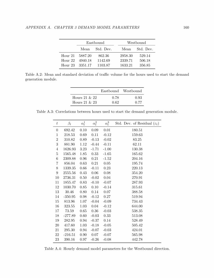
APPENDIX A. CHAPTER 3 DEMAND MODEL PARAMETERS 160
Eastbound Westbound
Mean Std. Dev. Mean Std. Dev.
Hour 21 5887.20 862.36 2958.30 529.14Hour 22 4940.18 1142.69 2339.71 506.18Hour 23 3351.17 1103.87 1633.21 356.85
Table A.2: Mean and standard deviation of traffic volume for the hours used to start the demandgeneration module.
Eastbound Westbound
Hours 21 & 22 0.78 0.93Hours 21 & 23 0.62 0.77
Table A.3: Correlations between hours used to start the demand generation module.
t βt α1t α2
t α3t Std. Dev. of Residual (εt)
0 692.42 0.10 0.09 0.01 180.511 218.53 0.69 0.11 -0.12 159.632 310.82 0.89 -0.13 -0.02 83.253 881.90 1.12 -0.44 -0.11 62.114 1626.93 3.23 -1.71 -1.00 130.385 1565.48 1.85 0.33 -1.65 165.626 2309.88 0.96 0.21 -1.52 204.167 856.04 0.63 0.21 0.05 195.748 1339.35 0.66 -0.11 0.23 220.139 2555.56 0.43 0.06 0.08 354.2010 2736.31 0.50 -0.02 0.04 270.9111 1855.47 0.83 -0.10 -0.07 287.9312 1030.70 0.85 0.10 -0.14 315.6113 30.46 0.80 0.14 0.07 388.5814 -350.95 0.98 -0.12 0.27 519.9415 813.96 1.07 -0.04 -0.09 734.4316 323.55 1.03 0.04 -0.12 644.0017 73.59 0.65 0.36 -0.03 538.3518 -277.89 0.60 -0.03 0.33 513.0819 282.95 0.94 -0.37 0.14 528.4920 417.60 1.03 -0.18 -0.05 505.4221 295.30 0.94 -0.07 -0.03 424.0122 -216.51 0.90 0.07 -0.07 565.9823 390.16 0.97 -0.26 -0.08 442.78
Table A.4: Hourly demand model parameters for the Westbound direction.
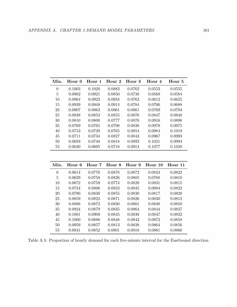
APPENDIX A. CHAPTER 3 DEMAND MODEL PARAMETERS 161
Min. Hour 0 Hour 1 Hour 2 Hour 3 Hour 4 Hour 5
0 0.1003 0.1020 0.0883 0.0762 0.0553 0.05555 0.0982 0.0921 0.0850 0.0738 0.0568 0.058410 0.0964 0.0923 0.0934 0.0762 0.0612 0.062515 0.0939 0.0948 0.0914 0.0784 0.0706 0.068820 0.0907 0.0863 0.0861 0.0861 0.0769 0.079425 0.0838 0.0853 0.0855 0.0876 0.0847 0.084830 0.0810 0.0800 0.0777 0.0876 0.0916 0.089635 0.0769 0.0765 0.0798 0.0838 0.0978 0.097540 0.0753 0.0729 0.0765 0.0854 0.0984 0.101945 0.0711 0.0734 0.0827 0.0843 0.0967 0.099350 0.0693 0.0748 0.0818 0.0892 0.1021 0.099455 0.0630 0.0695 0.0718 0.0914 0.1077 0.1028
Min. Hour 6 Hour 7 Hour 8 Hour 9 Hour 10 Hour 11
0 0.0614 0.0770 0.0878 0.0872 0.0824 0.08225 0.0629 0.0758 0.0826 0.0805 0.0768 0.081010 0.0672 0.0759 0.0774 0.0820 0.0831 0.081515 0.0724 0.0806 0.0823 0.0845 0.0804 0.082220 0.0790 0.0830 0.0855 0.0830 0.0817 0.082825 0.0859 0.0822 0.0871 0.0826 0.0830 0.081230 0.0886 0.0872 0.0830 0.0801 0.0838 0.085035 0.0924 0.0879 0.0835 0.0864 0.0844 0.083740 0.1001 0.0909 0.0845 0.0838 0.0847 0.083245 0.1000 0.0886 0.0848 0.0843 0.0872 0.085850 0.0959 0.0857 0.0813 0.0838 0.0864 0.085655 0.0941 0.0852 0.0801 0.0818 0.0861 0.0860
Table A.5: Proportion of hourly demand for each five-minute interval for the Eastbound direction.
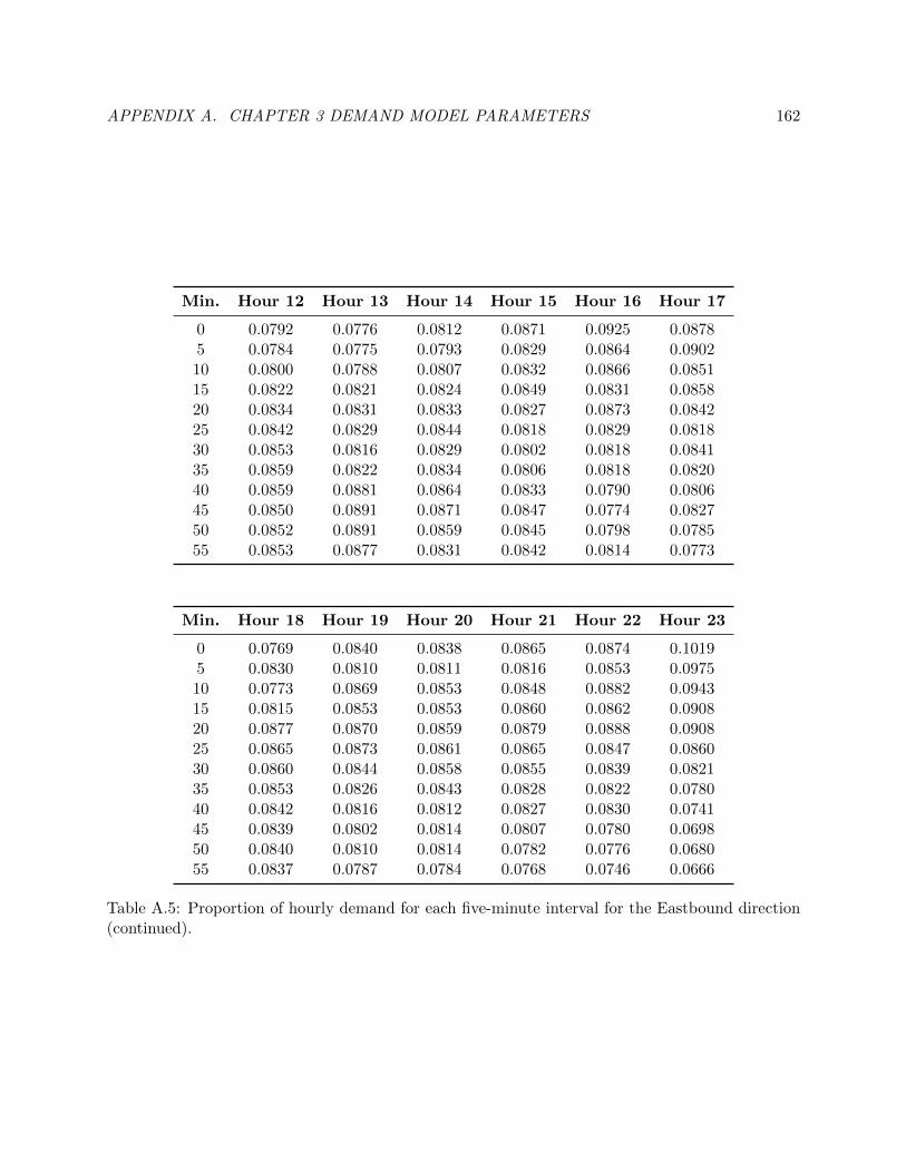
APPENDIX A. CHAPTER 3 DEMAND MODEL PARAMETERS 162
Min. Hour 12 Hour 13 Hour 14 Hour 15 Hour 16 Hour 17
0 0.0792 0.0776 0.0812 0.0871 0.0925 0.08785 0.0784 0.0775 0.0793 0.0829 0.0864 0.090210 0.0800 0.0788 0.0807 0.0832 0.0866 0.085115 0.0822 0.0821 0.0824 0.0849 0.0831 0.085820 0.0834 0.0831 0.0833 0.0827 0.0873 0.084225 0.0842 0.0829 0.0844 0.0818 0.0829 0.081830 0.0853 0.0816 0.0829 0.0802 0.0818 0.084135 0.0859 0.0822 0.0834 0.0806 0.0818 0.082040 0.0859 0.0881 0.0864 0.0833 0.0790 0.080645 0.0850 0.0891 0.0871 0.0847 0.0774 0.082750 0.0852 0.0891 0.0859 0.0845 0.0798 0.078555 0.0853 0.0877 0.0831 0.0842 0.0814 0.0773
Min. Hour 18 Hour 19 Hour 20 Hour 21 Hour 22 Hour 23
0 0.0769 0.0840 0.0838 0.0865 0.0874 0.10195 0.0830 0.0810 0.0811 0.0816 0.0853 0.097510 0.0773 0.0869 0.0853 0.0848 0.0882 0.094315 0.0815 0.0853 0.0853 0.0860 0.0862 0.090820 0.0877 0.0870 0.0859 0.0879 0.0888 0.090825 0.0865 0.0873 0.0861 0.0865 0.0847 0.086030 0.0860 0.0844 0.0858 0.0855 0.0839 0.082135 0.0853 0.0826 0.0843 0.0828 0.0822 0.078040 0.0842 0.0816 0.0812 0.0827 0.0830 0.074145 0.0839 0.0802 0.0814 0.0807 0.0780 0.069850 0.0840 0.0810 0.0814 0.0782 0.0776 0.068055 0.0837 0.0787 0.0784 0.0768 0.0746 0.0666
Table A.5: Proportion of hourly demand for each five-minute interval for the Eastbound direction(continued).
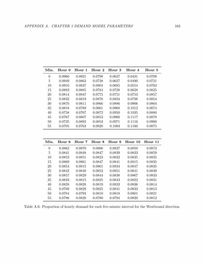
APPENDIX A. CHAPTER 3 DEMAND MODEL PARAMETERS 163
Min. Hour 0 Hour 1 Hour 2 Hour 3 Hour 4 Hour 5
0 0.0960 0.0921 0.0798 0.0637 0.0431 0.07095 0.0949 0.0863 0.0738 0.0627 0.0490 0.072110 0.0910 0.0837 0.0804 0.0685 0.0554 0.076315 0.0883 0.0885 0.0784 0.0728 0.0628 0.082520 0.0814 0.0847 0.0775 0.0751 0.0753 0.085725 0.0832 0.0819 0.0876 0.0834 0.0798 0.085430 0.0870 0.0811 0.0866 0.0886 0.0906 0.086435 0.0818 0.0789 0.0861 0.0968 0.1012 0.087440 0.0758 0.0767 0.0872 0.0950 0.1035 0.088045 0.0767 0.0807 0.0853 0.0960 0.1117 0.087850 0.0735 0.0892 0.0853 0.0971 0.1116 0.090055 0.0705 0.0763 0.0920 0.1003 0.1160 0.0875
Min. Hour 6 Hour 7 Hour 8 Hour 9 Hour 10 Hour 11
0 0.0862 0.0870 0.0866 0.0837 0.0850 0.08735 0.0841 0.0848 0.0847 0.0839 0.0833 0.085910 0.0853 0.0851 0.0823 0.0832 0.0835 0.083515 0.0869 0.0861 0.0847 0.0841 0.0815 0.083520 0.0854 0.0815 0.0861 0.0834 0.0847 0.083525 0.0842 0.0840 0.0853 0.0851 0.0841 0.083930 0.0857 0.0829 0.0844 0.0838 0.0867 0.083335 0.0833 0.0815 0.0825 0.0843 0.0822 0.083140 0.0828 0.0828 0.0819 0.0833 0.0836 0.081445 0.0789 0.0829 0.0825 0.0841 0.0833 0.081350 0.0784 0.0793 0.0810 0.0818 0.0801 0.082155 0.0786 0.0820 0.0780 0.0794 0.0820 0.0812
Table A.6: Proportion of hourly demand for each five-minute interval for the Westbound direction.
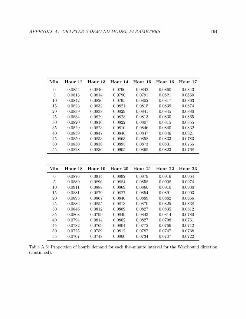
APPENDIX A. CHAPTER 3 DEMAND MODEL PARAMETERS 164
Min. Hour 12 Hour 13 Hour 14 Hour 15 Hour 16 Hour 17
0 0.0854 0.0846 0.0796 0.0842 0.0860 0.08435 0.0813 0.0814 0.0790 0.0791 0.0821 0.085010 0.0842 0.0826 0.0795 0.0802 0.0817 0.086315 0.0823 0.0832 0.0821 0.0815 0.0839 0.087420 0.0839 0.0838 0.0829 0.0841 0.0845 0.088025 0.0834 0.0829 0.0828 0.0813 0.0830 0.086530 0.0820 0.0816 0.0822 0.0807 0.0815 0.085535 0.0829 0.0823 0.0810 0.0846 0.0840 0.083240 0.0839 0.0847 0.0846 0.0847 0.0846 0.082145 0.0850 0.0853 0.0863 0.0858 0.0833 0.078350 0.0830 0.0838 0.0895 0.0873 0.0831 0.076555 0.0828 0.0836 0.0905 0.0865 0.0823 0.0768
Min. Hour 18 Hour 19 Hour 20 Hour 21 Hour 22 Hour 23
0 0.0876 0.0914 0.0892 0.0879 0.0916 0.09645 0.0889 0.0896 0.0884 0.0858 0.0908 0.097410 0.0911 0.0888 0.0869 0.0860 0.0910 0.093015 0.0881 0.0879 0.0827 0.0854 0.0891 0.090320 0.0895 0.0867 0.0840 0.0889 0.0882 0.086625 0.0886 0.0855 0.0813 0.0870 0.0825 0.083830 0.0846 0.0812 0.0809 0.0827 0.0835 0.081235 0.0808 0.0799 0.0849 0.0843 0.0814 0.078040 0.0794 0.0814 0.0802 0.0827 0.0798 0.076145 0.0782 0.0769 0.0804 0.0772 0.0766 0.071250 0.0725 0.0759 0.0812 0.0787 0.0747 0.073855 0.0707 0.0748 0.0800 0.0734 0.0707 0.0722
Table A.6: Proportion of hourly demand for each five-minute interval for the Westbound direction(continued).

APPENDIX B. CHAPTER 3 CONSUMER CHOICE MODELS 165
Appendix B
Chapter 3 Consumer Choice Models
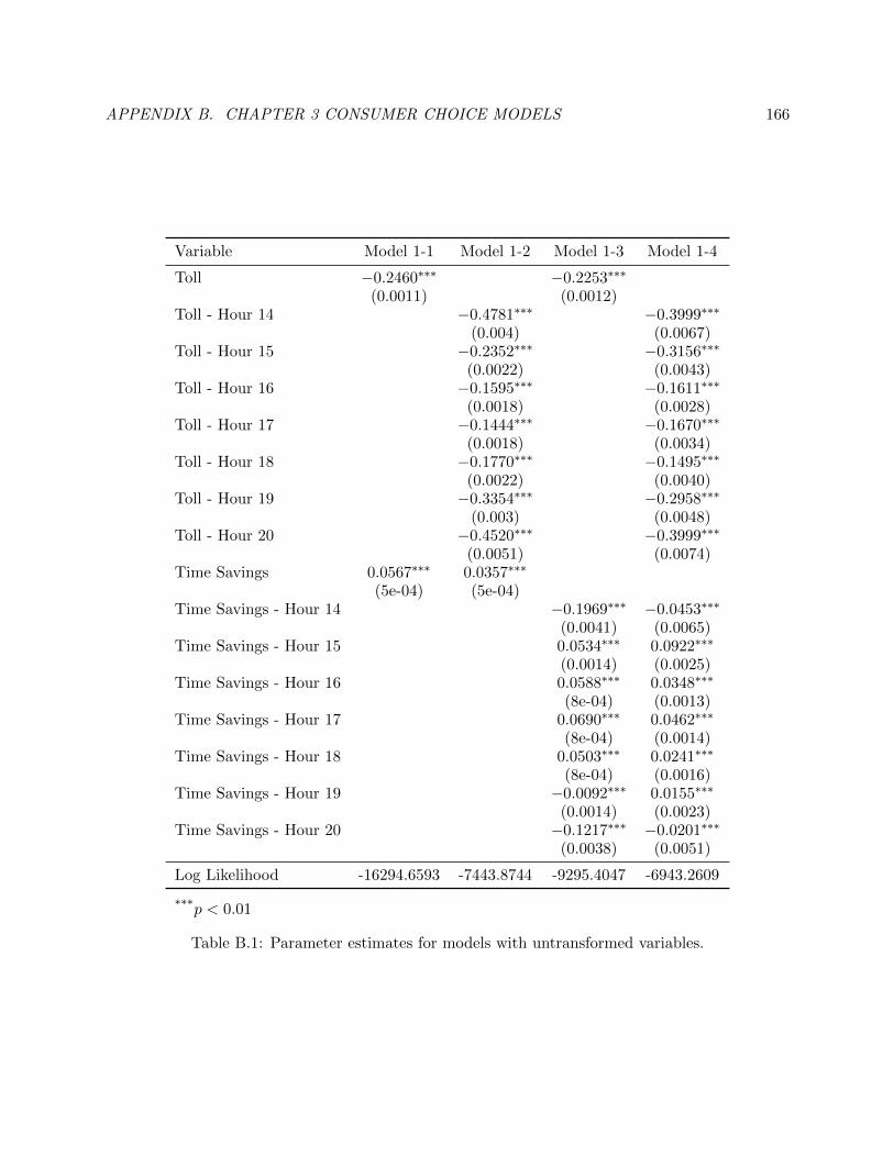
APPENDIX B. CHAPTER 3 CONSUMER CHOICE MODELS 166
Variable Model 1-1 Model 1-2 Model 1-3 Model 1-4
Toll −0.2460∗∗∗ −0.2253∗∗∗
(0.0011) (0.0012)Toll - Hour 14 −0.4781∗∗∗ −0.3999∗∗∗
(0.004) (0.0067)Toll - Hour 15 −0.2352∗∗∗ −0.3156∗∗∗
(0.0022) (0.0043)Toll - Hour 16 −0.1595∗∗∗ −0.1611∗∗∗
(0.0018) (0.0028)Toll - Hour 17 −0.1444∗∗∗ −0.1670∗∗∗
(0.0018) (0.0034)Toll - Hour 18 −0.1770∗∗∗ −0.1495∗∗∗
(0.0022) (0.0040)Toll - Hour 19 −0.3354∗∗∗ −0.2958∗∗∗
(0.003) (0.0048)Toll - Hour 20 −0.4520∗∗∗ −0.3999∗∗∗
(0.0051) (0.0074)Time Savings 0.0567∗∗∗ 0.0357∗∗∗
(5e-04) (5e-04)Time Savings - Hour 14 −0.1969∗∗∗ −0.0453∗∗∗
(0.0041) (0.0065)Time Savings - Hour 15 0.0534∗∗∗ 0.0922∗∗∗
(0.0014) (0.0025)Time Savings - Hour 16 0.0588∗∗∗ 0.0348∗∗∗
(8e-04) (0.0013)Time Savings - Hour 17 0.0690∗∗∗ 0.0462∗∗∗
(8e-04) (0.0014)Time Savings - Hour 18 0.0503∗∗∗ 0.0241∗∗∗
(8e-04) (0.0016)Time Savings - Hour 19 −0.0092∗∗∗ 0.0155∗∗∗
(0.0014) (0.0023)Time Savings - Hour 20 −0.1217∗∗∗ −0.0201∗∗∗
(0.0038) (0.0051)
Log Likelihood -16294.6593 -7443.8744 -9295.4047 -6943.2609
***p < 0.01
Table B.1: Parameter estimates for models with untransformed variables.
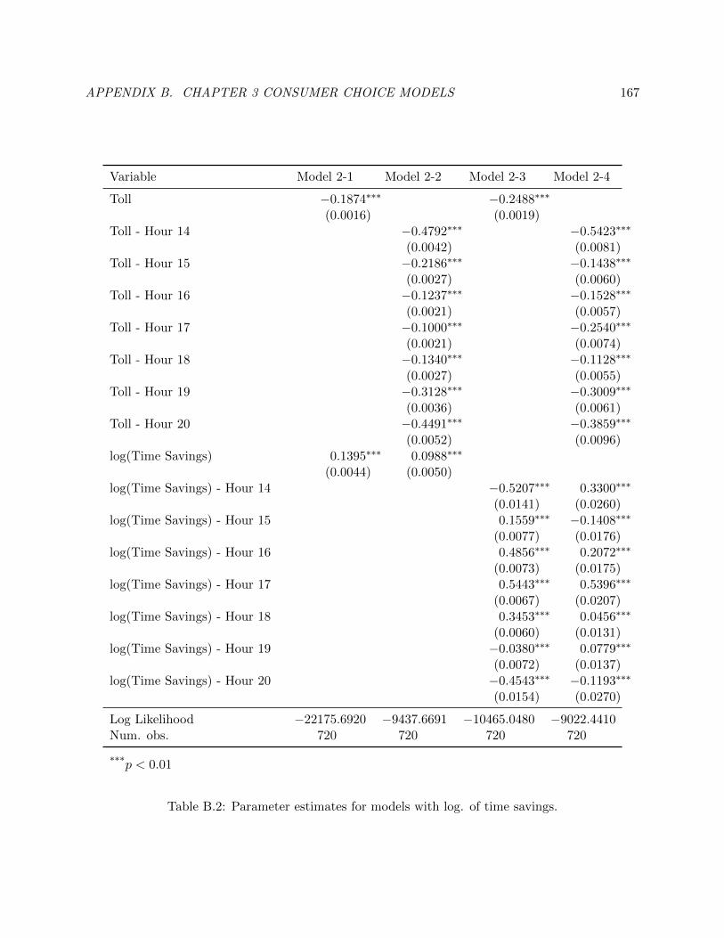
APPENDIX B. CHAPTER 3 CONSUMER CHOICE MODELS 167
Variable Model 2-1 Model 2-2 Model 2-3 Model 2-4
Toll −0.1874∗∗∗ −0.2488∗∗∗
(0.0016) (0.0019)Toll - Hour 14 −0.4792∗∗∗ −0.5423∗∗∗
(0.0042) (0.0081)Toll - Hour 15 −0.2186∗∗∗ −0.1438∗∗∗
(0.0027) (0.0060)Toll - Hour 16 −0.1237∗∗∗ −0.1528∗∗∗
(0.0021) (0.0057)Toll - Hour 17 −0.1000∗∗∗ −0.2540∗∗∗
(0.0021) (0.0074)Toll - Hour 18 −0.1340∗∗∗ −0.1128∗∗∗
(0.0027) (0.0055)Toll - Hour 19 −0.3128∗∗∗ −0.3009∗∗∗
(0.0036) (0.0061)Toll - Hour 20 −0.4491∗∗∗ −0.3859∗∗∗
(0.0052) (0.0096)log(Time Savings) 0.1395∗∗∗ 0.0988∗∗∗
(0.0044) (0.0050)log(Time Savings) - Hour 14 −0.5207∗∗∗ 0.3300∗∗∗
(0.0141) (0.0260)log(Time Savings) - Hour 15 0.1559∗∗∗ −0.1408∗∗∗
(0.0077) (0.0176)log(Time Savings) - Hour 16 0.4856∗∗∗ 0.2072∗∗∗
(0.0073) (0.0175)log(Time Savings) - Hour 17 0.5443∗∗∗ 0.5396∗∗∗
(0.0067) (0.0207)log(Time Savings) - Hour 18 0.3453∗∗∗ 0.0456∗∗∗
(0.0060) (0.0131)log(Time Savings) - Hour 19 −0.0380∗∗∗ 0.0779∗∗∗
(0.0072) (0.0137)log(Time Savings) - Hour 20 −0.4543∗∗∗ −0.1193∗∗∗
(0.0154) (0.0270)
Log Likelihood −22175.6920 −9437.6691 −10465.0480 −9022.4410Num. obs. 720 720 720 720
***p < 0.01
Table B.2: Parameter estimates for models with log. of time savings.

APPENDIX B. CHAPTER 3 CONSUMER CHOICE MODELS 168
Variable Model 3-1 Model 3-2 Model 3-3 Model 3-4
Toll −0.1954∗∗∗ −0.1882∗∗∗
(8e-04) (8e-04)Toll - Hour 14 −0.4547∗∗∗ −0.4153∗∗∗
(0.004) (0.0045)Toll - Hour 15 −0.1994∗∗∗ −0.2700∗∗∗
(0.0021) (0.0028)Toll - Hour 16 −0.1360∗∗∗ −0.1307∗∗∗
(0.0016) (0.0019)Toll - Hour 17 −0.1136∗∗∗ −0.1083∗∗∗
(0.0015) (0.0020)Toll - Hour 18 −0.1340∗∗∗ −0.1345∗∗∗
(0.0019) (0.0027)Toll - Hour 19 −0.2859∗∗∗ −0.2887∗∗∗
(0.0028) (0.0037)Toll - Hour 20 −0.4290∗∗∗ −0.4110∗∗∗
(0.0050) (0.0056)(Time Savings)2 0.0016∗∗∗ 0.0010∗∗∗
(1e-04) (1e-05)(Time Savings)2 - Hour 14 −0.0235∗∗∗ −0.0029∗∗∗
(6e-04) (6e-04)(Time Savings)2 - Hour 15 0.0033∗∗∗ 0.0045∗∗∗
(1e-04) (1e-04)(Time Savings)2 - Hour 16 0.0011∗∗∗ 6e− 04∗∗∗
(2e-05) (0.0000)(Time Savings)2 - Hour 17 0.0018∗∗∗ 9e− 04∗∗∗
(3e-05) (0.0000)(Time Savings)2 - Hour 18 0.0018∗∗∗ 9e− 04∗∗∗
(4e-05) (0.0000)(Time Savings)2 - Hour 19 −9e− 04∗∗∗ 0.0012∗∗∗
(1e-04) (1e-04)(Time Savings)2 - Hour 20 −0.0082∗∗∗ −0.0014∗∗∗
(3e-04) (3e-04)
Log Likelihood -15642.3036 -7174.4661 -12972.6198 -6309.6336Num. obs. 720 720 720 720
***p < 0.01
Table B.3: Parameters estimates for models with time savings squared.

APPENDIX C. CHAPTER 3 NUMERICAL STUDY DATA 169
Appendix C
Chapter 3 Numerical Study Data
Hour Certainty Eqv. (CE) Sample Avg. Appx. (SAA)
0 $ 5.06 $ 3.351 $ 4.37 $ 4.812 $ 4.36 $ 1.883 $ 4.32 $ 1.804 $ 3.31 $ 4.235 $ 2.71 $ 2.426 $ 2.80 $ 3.257 $ 3.74 $ 2.828 $ 3.01 $ 3.219 $ 4.25 $ 3.5710 $ 4.04 $ 2.5611 $ 4.91 $ 2.5712 $ 2.46 $ 3.0913 $ 2.52 $ 14.6814 $ 11.59 $ 30.5815 $ 14.43 $ 33.1916 $ 16.85 $ 32.5717 $ 12.14 $ 32.2218 $ 9.85 $ 19.9519 $ 5.76 $ 9.3520 $ 3.39 $ 3.6821 $ 3.68 $ 3.6422 $ 3.29 $ 3.4023 $ 4.46 $ 2.74
Table C.1: Starting points for the time-of-use policy.
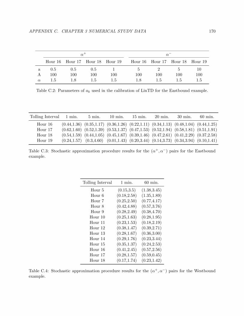
APPENDIX C. CHAPTER 3 NUMERICAL STUDY DATA 170
α+ α−
Hour 16 Hour 17 Hour 18 Hour 19 Hour 16 Hour 17 Hour 18 Hour 19
a 0.5 0.5 0.5 1 5 2 5 10A 100 100 100 100 100 100 100 100α 1.5 1.8 1.5 1.5 1.8 1.5 1.5 1.5
Table C.2: Parameters of ak used in the calibration of LinTD for the Eastbound example.
Tolling Interval 1 min. 5 min. 10 min. 15 min. 20 min. 30 min. 60 min.
Hour 16 (0.44,1.36) (0.35,1.17) (0.36,1.26) (0.22,1.11) (0.34,1.13) (0.48,1.04) (0.44,1.25)Hour 17 (0.62,1.60) (0.52,1.39) (0.53,1.37) (0.47,1.53) (0.52,1.94) (0.58,1.81) (0.51,1.91)Hour 18 (0.54,1.59) (0.44,1.05) (0.45,1.67) (0.39,1.46) (0.47,2.61) (0.41,2.29) (0.37,2.58)Hour 19 (0.24,1.57) (0.3,4.60) (0.01,1.43) (0.20,3.44) (0.14,3.73) (0.34,3.94) (0.10,1.41)
Table C.3: Stochastic approximation procedure results for the (α+, α−) pairs for the Eastboundexample.
Tolling Interval 1 min. 60 min.
Hour 5 (0.15,3.5) (1.38,3.45)Hour 6 (0.18,2.58) (1.35,1.89)Hour 7 (0.25,2.50) (0.77,4.17)Hour 8 (0.42,4.88) (0.57,3.76)Hour 9 (0.28,2.49) (0.38,4.70)Hour 10 (0.25,1.63) (0.28,1.95)Hour 11 (0.23,1.53) (0.18,2.19)Hour 12 (0.38,1.47) (0.39,2.71)Hour 13 (0.28,1.67) (0.36,3.00)Hour 14 (0.29,1.76) (0.23,3.44)Hour 15 (0.35,1.37) (0.24,2.53)Hour 16 (0.41,2.45) (0.57,2.56)Hour 17 (0.28,1.57) (0.59,0.45)Hour 18 (0.17,1.74) (0.23,1.42)
Table C.4: Stochastic approximation procedure results for the (α+, α−) pairs for the Westboundexample.

APPENDIX D. STATISTICAL ANALYSIS OF U.S. ELECTRICITY GENERATION 171
Appendix D
Statistical analysis of U.S. electricity
generation
In order to test whether unit size significantly affects the operational cost of a plant we analyzed
the following regression models:
avgUnitCost = β0 × avgGenSizeβ1 × capFactorβ2 × adjFuelCostβ3 × Effβ4
×N∏i=1
yearDummyβyearii (D.1)
avgUnitCost− avgLaborCost = γ0 × avgGenSizeγ1 × capFactorγ2 × adjFuelCostγ3 × Effγ4
×N∏i=1
yearDummyγyearii (D.2)
The definition of the variables used in the regression model above can be found in Table D.1. The
first model is used to analyze the total unit operating cost of power plants, whereas the second
model only looks at the non-labor portion of a plant’s operating costs. These two models were
tested for four different generation technologies: combined cycle, coal, gas turbines and nuclear.
The operational data on electric generating facilities was found in the annual filings to the Fed-
eral Energy Regulatory Commission (FERC) by the major utilities (FERC, 2010) for the year 2010.
A data point includes information regarding employee count, capacity, age of the generator, fuel
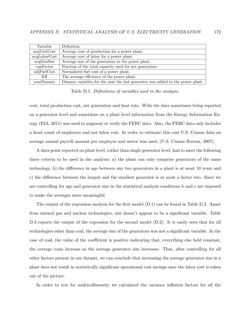
APPENDIX D. STATISTICAL ANALYSIS OF U.S. ELECTRICITY GENERATION 172
Variable DefinitionavgUnitCost Average cost of production for a power plant.
avgLaborCost Average cost of labor for a power plant.avgGenSize Average size of the generators in the power plant.capFactor Fraction of the total capacity used for net generation.
adjFuelCost Normalized fuel cost of a power plant.Eff The average efficiency of the power plant.
yearDummy Dummy variables for the year the last generator was added to the power plant.
Table D.1: Definitions of variables used in the analysis.
cost, total production cost, net generation and heat rate. With the data sometimes being reported
on a generator level and sometimes on a plant level information from the Energy Information En-
ergy (EIA, 2011) was used to augment or verify the FERC data. Also, the FERC data only includes
a head count of employees and not labor cost. In order to estimate this cost U.S. Census data on
average annual payroll amount per employee and sector was used, (U.S. Census Bureau, 2007).
A data point reported on plant level, rather than single generator level, had to meet the following
three criteria to be used in the analysis; a) the plant can only comprise generators of the same
technology, b) the difference in age between any two generators in a plant is at most 10 years and
c) the difference between the largest and the smallest generator is at most a factor two. Since we
are controlling for age and generator size in the statistical analysis conditions b and c are imposed
to make the averages more meaningful.
The output of the regression analysis for the first model (D.1) can be found in Table D.2. Apart
from natural gas and nuclear technologies, size doesn’t appear to be a significant variable. Table
D.3 reports the output of the regression for the second model (D.2). It is easily seen that for all
technologies other than coal, the average size of the generators was not a significant variable. In the
case of coal, the value of the coefficient is positive indicating that, everything else held constant,
the average costs increase as the average generator size increases. Thus, after controlling for all
other factors present in our dataset, we can conclude that increasing the average generator size in a
plant does not result in statistically significant operational cost savings once the labor cost is taken
out of the picture.
In order to test for multicollinearity we calculated the variance inflation factors for all the
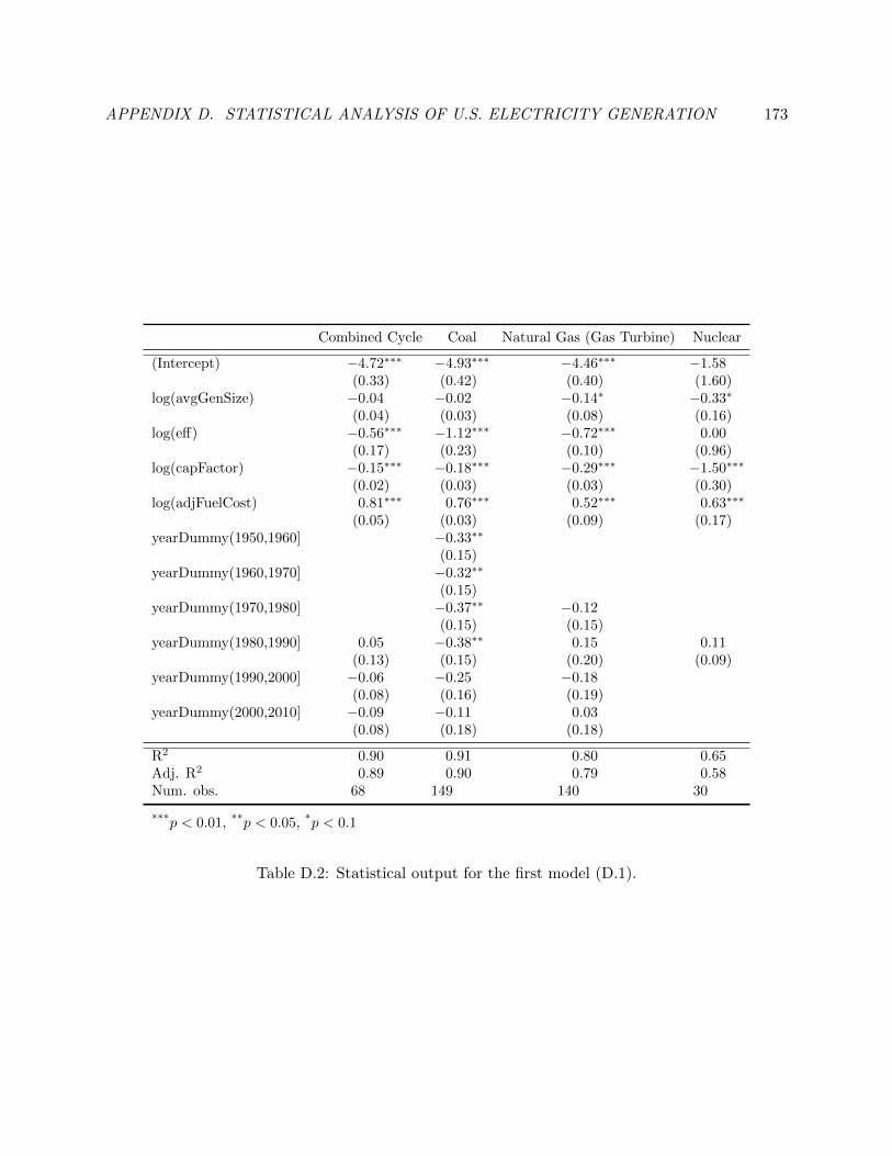
APPENDIX D. STATISTICAL ANALYSIS OF U.S. ELECTRICITY GENERATION 173
Combined Cycle Coal Natural Gas (Gas Turbine) Nuclear
(Intercept) −4.72∗∗∗ −4.93∗∗∗ −4.46∗∗∗ −1.58(0.33) (0.42) (0.40) (1.60)
log(avgGenSize) −0.04 −0.02 −0.14∗ −0.33∗
(0.04) (0.03) (0.08) (0.16)log(eff) −0.56∗∗∗ −1.12∗∗∗ −0.72∗∗∗ 0.00
(0.17) (0.23) (0.10) (0.96)log(capFactor) −0.15∗∗∗ −0.18∗∗∗ −0.29∗∗∗ −1.50∗∗∗
(0.02) (0.03) (0.03) (0.30)log(adjFuelCost) 0.81∗∗∗ 0.76∗∗∗ 0.52∗∗∗ 0.63∗∗∗
(0.05) (0.03) (0.09) (0.17)yearDummy(1950,1960] −0.33∗∗
(0.15)yearDummy(1960,1970] −0.32∗∗
(0.15)yearDummy(1970,1980] −0.37∗∗ −0.12
(0.15) (0.15)yearDummy(1980,1990] 0.05 −0.38∗∗ 0.15 0.11
(0.13) (0.15) (0.20) (0.09)yearDummy(1990,2000] −0.06 −0.25 −0.18
(0.08) (0.16) (0.19)yearDummy(2000,2010] −0.09 −0.11 0.03
(0.08) (0.18) (0.18)
R2 0.90 0.91 0.80 0.65Adj. R2 0.89 0.90 0.79 0.58Num. obs. 68 149 140 30
***p < 0.01, **p < 0.05, *p < 0.1
Table D.2: Statistical output for the first model (D.1).

APPENDIX D. STATISTICAL ANALYSIS OF U.S. ELECTRICITY GENERATION 174
Combined Cycle Coal Natural Gas (Gas Turbine) Nuclear
(Intercept) −4.73∗∗∗ −5.97∗∗∗ −4.84∗∗∗ −4.83∗
(0.34) (0.51) (0.64) (2.42)log(avgGenSize) −0.02 0.06∗ 0.00 0.06
(0.04) (0.03) (0.12) (0.25)log(eff) −0.47∗∗ −1.52∗∗∗ −0.78∗∗∗ −0.22
(0.18) (0.27) (0.16) (1.45)log(capFactor) −0.12∗∗∗ −0.07∗ −0.22∗∗∗ −1.71∗∗∗
(0.02) (0.04) (0.05) (0.45)log(adjFuelCost) 0.81∗∗∗ 0.87∗∗∗ 0.62∗∗∗ 0.77∗∗∗
(0.06) (0.04) (0.14) (0.26)yearDummy(1950,1960] −0.34∗
(0.18)yearDummy(1960,1970] −0.34∗
(0.18)yearDummy(1970,1980] −0.42∗∗ −0.42∗
(0.18) (0.24)yearDummy(1980,1990] 0.00 −0.46∗∗ −0.11 −0.03
(0.14) (0.18) (0.32) (0.13)yearDummy(1990,2000] −0.09 −0.26 −0.54∗
(0.08) (0.19) (0.29)yearDummy(2000,2010] −0.12 −0.16 −0.41
(0.08) (0.21) (0.29)
R2 0.88 0.87 0.59 0.51Adj. R2 0.87 0.86 0.57 0.40Num. obs. 68 149 140 30
***p < 0.01, **p < 0.05, *p < 0.1
Table D.3: Statistical output for the second model (D.2).

APPENDIX D. STATISTICAL ANALYSIS OF U.S. ELECTRICITY GENERATION 175
Variable Name Combined Cycle Coal Natural Gas (GT) Nuclear
log(avgGenSize) 2.26 4.76 2.10 1.72log(eff) 2.42 3.95 1.86 1.34
log(capFactor) 1.92 2.05 1.79 1.21log(adjFuelCost) 1.11 1.76 1.16 1.11
yearDummy 2.03 3.31 2.60 1.72
Table D.4: Variance inflation factors.
variables. Table D.4 reports variance inflation factors for all variables in all datasets. As it can be
seen from the table, multicollinearity does not appear to be a significant issue in our model.