informed source separation for multiple instruments of...

“thesis” — 2013/9/1 — 14:45 — page 1 — #1

Informed Source Separation for Multiple Instruments of Similar Timbre

Jakue López Armendáriz

MASTER THESIS UPF / 2013 Master in Sound and Music Computing

Master thesis supervisor: Dr. Jordi Janer

Department of Information and Communication Technologies Universitat Pompeu Fabra, Barcelona

“thesis” — 2013/9/1 — 14:45 — page i — #2

i

“thesis” — 2013/9/1 — 14:45 — page ii — #3

Copyright: c© 2013 Jakue Lopez Armendariz. This is an open-access documentdistributed under the terms of the Creative Commons Attribution License 3.0Unported, which permits unrestricted use, distribution, and reproduction in anymedium, provided the original author and source are credited.

ii

“thesis” — 2013/9/1 — 14:45 — page iii — #4

Acknowledgements

I would first like to thank Prof. Xavier Serra for giving me the opportunity tojoin the SMC Master’s program at the Pompeu Fabra University (UPF) and to allthe people from the Music Technology Group (MTG), specially the members andSMC students which have helped and influenced the development of this work.

I owe my deepest gratitude to my supervisor, Dr. Jordi Janer, whose exper-tise, understanding and patience made possible the writing of this thesis. I reallyappreciate his knowledge and his assistance during this time.

I would like to thank my parents for the support they provide through my entirelife. Mila esker Aita eta Ama.

I would also like to thank my girlfriend, because she does not only give un-limited help and support, but she also brings optimism and happiness into my life.Nagyon koszonom Orsi.

To all of you.Thanks.

iii

“thesis” — 2013/9/1 — 14:45 — page iv — #5

AbstractThis Master’s thesis focuses on the challenging task of separating the musicalaudio sources with instruments of similar timbre. We address the case in whichexternal pitch information to assist the separation process is available. This in-formation is provided to the source / filter model, which is embedded in a Non-Negative Matrix Factorization (NMF) framework that processes the audio inputspectrogram. Different state of the art literature methods are inspected and ex-tended. As an extension to these, two new separation methods are proposed, theMulti-Excitation and Single Filter Instantaneous Mixture Model and the Multi-Excitation and Multi-Filter Instantaneous Mixture Model. The use of dedicatedsource and filter decomposition for each instrument is proposed. In addition, weintroduce the use of timbre models in the separation process. Timbre modelsare previously trained on isolated instrument recordings. The methods are com-pared with the BSS Eval and PEASS evaluation toolkits over an existing dataset.Promising results obtained in the conducted experiments, which shows that this isa path to be further investigated.

iv

“thesis” — 2013/9/1 — 14:45 — page v — #6

Contents

Index of figures viii

Index of tables xi

1 INTRODUCTION 1

2 STATE OF THE ART 32.1 Source Separation . . . . . . . . . . . . . . . . . . . . . . . . . . 3

2.1.1 Models and Methods . . . . . . . . . . . . . . . . . . . . 52.2 Musical Audio Source Separation . . . . . . . . . . . . . . . . . 9

2.2.1 Instantaneous Mixture Model . . . . . . . . . . . . . . . 102.2.2 Multi-Excitation Model . . . . . . . . . . . . . . . . . . 14

2.3 Bowed String Instrument Modeling . . . . . . . . . . . . . . . . 172.3.1 Physics and Models of Violin Family Instruments . . . . . 172.3.2 Source / Filter Modeling . . . . . . . . . . . . . . . . . . 19

3 METHODOLOGY 213.1 First approach: Modifications over the IMM . . . . . . . . . . . . 21

3.1.1 Source Model . . . . . . . . . . . . . . . . . . . . . . . . 213.2 Proposed Extensions: Combining IMM and Multi-Excitation Model 24

3.2.1 Multi-Excitation and Single Filter IMM . . . . . . . . . . 243.2.2 Multi-Excitation and Multi-Filter IMM . . . . . . . . . . 25

3.3 Supervised Timbre Models . . . . . . . . . . . . . . . . . . . . . 27

4 EVALUATION AND RESULTS 304.1 Evaluation Metrics . . . . . . . . . . . . . . . . . . . . . . . . . 30

4.1.1 The BSS EVAL Toolbox . . . . . . . . . . . . . . . . . . 304.1.2 The PEASS Toolkit . . . . . . . . . . . . . . . . . . . . . 31

4.2 Description of the Dataset . . . . . . . . . . . . . . . . . . . . . 324.3 Evaluation Methodology and Results . . . . . . . . . . . . . . . . 33

4.3.1 Comparison of IMM and the Proposed Models . . . . . . 33

v

“thesis” — 2013/9/1 — 14:45 — page vi — #7

4.3.2 Multi-Excitation and Multi-Filter Model Parameter Opti-mization . . . . . . . . . . . . . . . . . . . . . . . . . . 38

4.3.3 Multi-Excitation and Multi-Filter Model with SupervisedTimbre Model Extension . . . . . . . . . . . . . . . . . . 41

5 CONCLUSIONS AND FUTURE WORK 515.1 Contributions . . . . . . . . . . . . . . . . . . . . . . . . . . . . 515.2 Conclusions . . . . . . . . . . . . . . . . . . . . . . . . . . . . . 525.3 Future work . . . . . . . . . . . . . . . . . . . . . . . . . . . . . 53

5.3.1 Source / Filter Model Improvements . . . . . . . . . . . . 535.3.2 Trained Filter Models Improvements . . . . . . . . . . . . 53

A APPENDIX A 55

B APPENDIX B 61

vi

“thesis” — 2013/9/1 — 14:45 — page vii — #8

List of Figures

2.1 Source / filter + accompaniment diagram of the IMM . . . . . . . 112.2 Solo/Accompaniment algorithm outline [Durrieu et al., 2009a] . . 132.3 Resonance curve of a typical violin body defined as the mechani-

cal input admittance at the bridge [Fletcher, 1999] . . . . . . . . . 19

3.1 Example of an WF0 basis generated with the glottal source model . 223.2 Source / filter + accompaniment diagram of the modified IMM . . 233.3 Multi-Excitation and Single Filter IMM diagram . . . . . . . . . 253.4 Multi-Excitation and Multi-Filter IMM diagram . . . . . . . . . . 263.5 Timber model Wφ bases decomposed into an smooth filter dictio-

nary bases WΓ and its gains HΓ. . . . . . . . . . . . . . . . . . . 273.6 Timbre matrices example over a cello excerpt. Smooth filter dic-

tionary bases WΓ (top), its activations HΓ (middle) and the ob-tained bases Wφ . . . . . . . . . . . . . . . . . . . . . . . . . . . 28

3.7 Timbre matrices example over a violin excerpt. Smooth filter dic-tionary bases WΓ (top), its activations HΓ (middle) and the ob-tained bases Wφ . . . . . . . . . . . . . . . . . . . . . . . . . . . 29

3.8 Multi-Excitation and Multi-Filter IMM diagram with supervisedfilters loaded . . . . . . . . . . . . . . . . . . . . . . . . . . . . . 29

4.1 Overall Perceptual Score (OPS) results by model for the Schubertaudio excerpt . . . . . . . . . . . . . . . . . . . . . . . . . . . . 37

4.2 Overall Perceptual Score (OPS) results by model for the Mozartaudio excerpt . . . . . . . . . . . . . . . . . . . . . . . . . . . . 37

4.3 Pitch estimations of a 8 second violin excerpt (Schubert record-ing). Estimations with Yin (top), MEF IMM (middle) and MEFIMM loading supervised timbre models (bottom). . . . . . . . . . 49

4.4 Pitch estimations over a 8 second cello excerpt (Schubert record-ing). Estimations with Yin (top), MEF IMM (middle) and MEFIMM loading supervised timbre models (bottom). . . . . . . . . . 49

vii

“thesis” — 2013/9/1 — 14:45 — page viii — #9

4.5 Pitch estimations over a 8 second viola excerpt (Mozart record-ing). Estimations with Yin (top), MEF IMM (middle) and MEFIMM loading supervised timbre models (bottom). . . . . . . . . . 50

4.6 Pitch estimations over a 8 second clarinet excerpt (Mozart record-ing). Estimations with Yin (top), MEF IMM (middle) and MEFIMM loading supervised timbre models (bottom). . . . . . . . . . 50

viii

“thesis” — 2013/9/1 — 14:45 — page ix — #10

List of Tables

4.1 SDR score results by model for the Schubert audio excerpt . . . . 344.2 SIR score results by model for the Schubert audio excerpt . . . . . 344.3 SAR score results by model for the Schubert audio excerpt . . . . 354.4 SDR score results by model for the Mozart audio excerpt . . . . . 354.5 SIR score results by model for the Mozart audio excerpt . . . . . 354.6 SAR score results by model for the Mozart audio excerpt . . . . . 364.7 PEASS toolkit results by model for the Schubert audio excerpt . . 374.8 PEASS toolkit results by model for the Mozart audio excerpt . . . 384.9 SDR score results by iteration over 90 P smooth filters and 20 K

bases . . . . . . . . . . . . . . . . . . . . . . . . . . . . . . . . . 394.10 SDR score results by P smooth filters over 30 iterations and 20 K

bases . . . . . . . . . . . . . . . . . . . . . . . . . . . . . . . . . 404.11 SDR score results by K bases over 90 P smooth filters and 30

iterations . . . . . . . . . . . . . . . . . . . . . . . . . . . . . . 404.12 Best parameter configuration over different tested K bases, P

smooth filters and iterations values . . . . . . . . . . . . . . . . . 404.13 BSSEval results of the Schubert recording for the Multi-Excitation

and Multi-Filter Model with estimated filters (MEF IMM), su-pervised filters (MEF IMM + SV FILT.) and unsupervised filters(MEF IMM + USV FILT.) . . . . . . . . . . . . . . . . . . . . . 42

4.14 BSSEval results of the Mozart recording for the Multi-Excitationand Multi-Filter Model with estimated filters (MEF IMM), su-pervised filters (MEF IMM + SV FILT.) and unsupervised filters(MEF IMM + USV FILT.) . . . . . . . . . . . . . . . . . . . . . 42

4.15 SDR score of the Schubert recording for the Multi-Excitation andMulti-Filter Model with estimated filters and supervised filters fordifferent iteration values . . . . . . . . . . . . . . . . . . . . . . 44

4.16 SDR score of the Mozart recording for the Multi-Excitation andMulti-Filter Model with estimated filters and supervised filters fordifferent iteration values . . . . . . . . . . . . . . . . . . . . . . 45

ix

“thesis” — 2013/9/1 — 14:45 — page x — #11

4.17 SDR score of the Schubert recording for the Multi-Excitation andMulti-Filter Model with estimated filters and supervised filters fordifferent block size values . . . . . . . . . . . . . . . . . . . . . . 46

4.18 SDR score of the Mozart recording for the Multi-Excitation andMulti-Filter Model with estimated filters and supervised filters fordifferent block size values . . . . . . . . . . . . . . . . . . . . . . 47

A.1 BSS Eval results for the Schubert excerpt over 10 iterations anddifferent values for P smooth filters and K bases . . . . . . . . . 56





B.1 SIR error of the Schubert recording for the Multi-Excitation andMulti-Filter Model with estimated filters and trained filters for dif-ferent iteration values . . . . . . . . . . . . . . . . . . . . . . . . 62

B.2 SIR error of the Mozart recording for the Multi-Excitation andMulti-Filter Model with estimated filters and trained filters for dif-ferent iteration values . . . . . . . . . . . . . . . . . . . . . . . . 63

B.3 SAR error of the Schubert recording for the Multi-Excitation andMulti-Filter Model with estimated filters, trained filters for differ-ent iteration values . . . . . . . . . . . . . . . . . . . . . . . . . 64

B.4 SAR error of the Mozart recording for the Multi-Excitation andMulti-Filter Model with estimated filters and trained filters for dif-ferent iteration values . . . . . . . . . . . . . . . . . . . . . . . . 65

B.5 SIR error of the Schubert recording for the Multi-Excitation andMulti-Filter Model with estimated filters and trained filters for dif-ferent block size values . . . . . . . . . . . . . . . . . . . . . . . 66

B.6 SIR error of the Mozart recording for the Multi-Excitation andMulti-Filter Model with estimated filters and trained filters for dif-ferent block size values . . . . . . . . . . . . . . . . . . . . . . . 67

B.7 SAR error of the Schubert recording for the Multi-Excitation andMulti-Filter Model with estimated filters and trained filters for dif-ferent block size values . . . . . . . . . . . . . . . . . . . . . . . 68

x

“thesis” — 2013/9/1 — 14:45 — page xi — #12

B.8 SAR error of the Mozart recording for the Multi-Excitation andMulti-Filter Model with estimated filters and trained filters for dif-ferent block size values . . . . . . . . . . . . . . . . . . . . . . . 69

xi

“thesis” — 2013/9/1 — 14:45 — page 1 — #13

Chapter 1

INTRODUCTION

Computational analysis of audio signals where multiple sources are present is achallenging problem. This task, which is defined as Source Separation (SS), couldbe solved by applying methods that separate the signals of individual sources fromthe original mixture. This well known technique to isolate the components from amixture has been demonstrated to be achievable.

The source separation problem is ubiquitous in many different application ar-eas as, for example: Audio Processing, Image processing, Chemometris or Bioin-formatics. In audio signal processing, there are many tasks where sound sourceseparation can be used, but the performance of the existing algorithms is still lim-ited compared to the human auditory system. Human listeners are able to perceiveand discriminate individual sources in complex mixtures. Based on the soundsegregation ability in humans several algorithms have been proposed. Specially,when the signals are composed by sources of similar characteristics, i.e. instru-ments of similar timbre, the estimation of an individual source from the acousticsignal mixture is disturbed by other coexisting sounds.

One of the divisions for source separation methods is done considering theprior available information. The different approaches can be divided into blindand non-blind. Blind Source Separation (BSS) denotes the separation of com-pletely unknown sources without using additional information. Non-blind or In-formed Source Separation (ISS) denotes the separation of sources for which fur-ther information is available, either for the individual sources or for the mixture.

More precisely, the work will focus on the separation for multiple instrumentsof similar timbre, having a String Quartet as a use case. In a set of instrumentslike the one here addressed there is an absence of a main or lead instrument andthe harmonicity between sources is high.

1

“thesis” — 2013/9/1 — 14:45 — page 2 — #14

The attempt of this thesis is to improve the quality of the separation. For sometechniques the required information for the separation of audio signals is the pitchof each source. In complex mixtures one way of obtaining this information isperforming a multi-pitch estimation. However, this task has turned to be a chal-lenging problem too.

For this reason, Informed Source Separation techniques are considered in here.As the goal is to provide a potentially higher quality result, the multi-pitch estima-tion step is avoided. The additional information that is used contains informationof the melody or pitch for each of the audio signal sources, (i.e. an aligned pitch-contour signal). This approach could be considered similar to the use of symbolicinformation of the pitch (e.g., an aligned score), an approach that has already beenaddressed in the literature under the name of Score-Informed Source Separation.In contrary, for the case addressed in this work, this kind of informed SS could benamed as Pitch-Informed Source Separation.

For facilitating this task various multimodal datasets are available. Besides thegeneral mixture audio recordings, even if not all the information is utilized, moreprior information is available. For example: pitch information (scores, pick-puprecordings), gestures (vide recordings) or spatial cues (binaural recordings).

Moreover, The Music Technology Group of the Universitat Pompeu Fabra,where this thesis has been carried out, is the main coordinator of the Performancesas Highly Enriched aNd Interactive Concert eXperiences (PHENICX) project.The MTG provides the project with expertise coming from different research ar-eas, being audio source separation one of them. For this reason, this work couldbe potentially useful as a first exploration for future applications in this project.

2

“thesis” — 2013/9/1 — 14:45 — page 3 — #15

Chapter 2

STATE OF THE ART

In this chapter, the theoretical background and a review on the relevant work forthis thesis is presented. First, the general concepts and methods for source separa-tion are introduced. Second, a more specific view on musical audio source sepa-ration is exposed. Finally, some of the physical / acoustic principles and modelingapproaches for bowed string instrument are introduced.

2.1 Source SeparationSource separation is the challenging problem of extracting individual signals froman observed mixture by computational means. It is usefully applied in many dif-ferent fields and types of signals such as image, video, medical, financial or radio.This work focuses on the separation of audio signals, and more specifically ofmusic audio signals.

The source separation task was first formulated in the mid 1980’s within a sta-tistical framework by [Herault et al., 1985]. In the early 1990’s, the introductionof Independent Component Analysis (ICA) by [Comon, 1994] and the appearanceof other related techniques set the ground for the development of the topic.

More specifically, in the field of auditory perception, [Bregman, 1990] pro-posed a cognitive approach for describing hearing complex auditory environ-ments, which increased the interest of the research community. This process,named as Auditory Scene Analysis (ASA), explains the steps required for the hu-man auditory system to analyze mixtures of sounds and recover descriptions ofindividual sounds. The work provided the basis for the computational imple-mentation of algorithms that approximate the sound separation capabilities of thehuman auditory system, concept known as Computational Auditory Scene Analy-sis (CASA). At the same time, both works on ICA and ASA set the beginning oftwo new approaches to acoustic separation: statistical/mathematical and biolog-

3

“thesis” — 2013/9/1 — 14:45 — page 4 — #16

ically inspired approaches. [Wang and Brown, 2006] presented a detailed litera-ture review on the different approaches that have been proposed to deal with thecomputational modeling of ASA.

The difficulty of a source separation problem is mainly determined by threefactors. First, the proportion between the number of mixture channels and thenumber of original sources determines it . The separation is easier if the observedmixture has more channels, or the same number of channels, than there are sourcesto separate. Second, the nature, i.e., complexity, of the mixture. Third, the amountof information about the sources or the mixture available a priori.

We don’t find a generalized agreement in the literature when assigning labels,neither according to all the different existing methods, nor according to the differ-ent degrees of knowledge available. However, nomenclature overviews proposedby authors like [Vincent et al., 2003] or [Burred, 2009] are reviewed in this sec-tion.

According to the proportion between the number of mixture channels and thenumber of original sources, Burred names the cases as over-determined, even-determined and undetermined source separation. He defines the task as over-determined when the observed mixture has more channels than sources. Even-determined (or determined) source separation corresponds to the case when thereare the same numbers of channels than sources to separate. In mixtures with lesschannels than sources, named as undetermined, additional difficulties, such asstronger assumptions, are often to be addressed.

Depending on the a priori information (i.e., given knowledge) available aboutthe sources or the mixture there is a distinction between blind, semi-blind andnon-blind source separation. The task is said to be blind if there is little or noknowledge available before the observation of the mixture. Particularly, BlindSource Separation (BSS) has become a standard nomenclature in the literature todenote the statistical methods that approach this case. However, it is to be men-tioned, that there is no strictly blind system due to the fact that, at least, somegeneral probabilistic assumptions like statistical independence and sparsity mustbe taken. ICA and sparsity-based methods (e.g., time-frequency masking) areincluded in here. When talking about Semi-blind Source Separation (SBSS), herefers to methods that include sinusoidal models and supervised methods wherethe source models are learned in advance. At last, Non-blind or, as it will bereferred in this document, Informed Source Separation (ISS), corresponds to sys-tems that, besides the mixture, they have detailed high level information about thesources or mixture as an input. This information can be, for example, the numberand kind of sources. More specifically, for musical source separation, the a prioriinformation can be of the kind of the score, a MIDI sequence, pitch-contour or anyother kind of detailed information of the melody been played. Also, another casecontained in here is where the information is extracted from the original isolated

4

“thesis” — 2013/9/1 — 14:45 — page 5 — #17

tracks that are encoded and embedded in the mixture (e.g., using watermarking).This information is later used in the separations stage to provide a higher qualityseparation [Liutkus et al., 2012]. ISS will be the case addressed in this work.

In the more specific context of audio source separation, Vincent proposed adivision between Audio Quality Oriented (AQO) and Significance Oriented (SO)applications. On the one hand, AQO has the goal of fully unmixing the individualsources present in the mixture with the highest possible quality. In this case, theoutput signals are intended to be listened to. Some AQO applications, as the oneto be addressed in this document, look for a fully unmixing of the original mixtureinto separated sources that are aimed to be listened separately. This turns to bethe most demanding application scenario, as the goal is to obtain a multitrackrecording equivalent to the one created for the final mix of the mixture. Ideally,the separated tracks should have the same or similar quality than they would havehad if recorded separately.

On the other hand, SO methods don’t require such a high quality separation,since the goal is to facilitate a high-level, semantic feature extraction from thesources. SO involves many tasks from the Music Information Retrieval field. Forexample, polyphonic transcription, or the task of automatically extracting the mu-sic score from the mixture, is a high demanding task included in SO application.It is worth mentioning that, obviously, AQO methods are also valid for the SOcontext too.

2.1.1 Models and MethodsAs mentioned before, source separation can be defined as the task of estimatingone ore more of the original source signals sm(n) from the observed mixture sig-nal x(n). When several sources are present simultaneously, the mixture x(n) canbe defined as

x(n) =M∑m=1

sm(n) (2.1)

where sm is the mth source signal and M is the number of sources.Several probabilistic approaches to source separation have been proposed in

the literature. The techniques about to be presented are very versatile and can belikely used in various applications with different purposes.

Signal Representation

It has to be mentioned that the separation is usually not computed directly fromthe original representation of the signal. In contrary, the signal is transformed to

5

“thesis” — 2013/9/1 — 14:45 — page 6 — #18

another kind of representation to fulfill certain goals. [Schmidt, 2008] describesthe following four considerations to signal representation.

First, to make explicit the desired characteristics of the signal. A representa-tion different from the original, e.g., the Fourier transform, which emphasizes themeaningful characteristics of it could help in the task of separating the sources.

Second, to introduce invariances with the goal to decrease the adverse charac-teristics that are known to be not relevant to separate the signals, e.g., the use ofpower spectrum that ignores the phase, which introduces an invariance to phaseshift.

Third, most of the approaches have the common goal of reducing the dimen-sionality of the data in order to reduce the computational cost. An example on oneof the most common techniques for dimensionality reduction, Principal Compo-nent Analysis (PCA) is presented in 2.1.1.

Finally, to allow signal reconstruction. A distinction between reversible (loss-less) and non-reversible (lossy) is made. In both cases the signals are separatedin the representation domain. In the lossless case, the representation is inverted toobtain the separated signals in the original domain. However, in the lossy case,the separated signals must be reconstructed in the original signal domain. A fil-tering applied to the signal mixture is done to achieve this. A common practice isto use time varying Wiener filters [Hopgood and Rayner, 2003]. The selection ofthe signal representation is important, since it determines how accurate the signalreconstruction could be.

Principal Component Analysis, Independent Component Analysis and Inde-pendent Subspace Analysis

Principal Component Analysis (PCA), Independent Component Analysis (ICA)and Independent Subspace Analysis (ISA) are very popular dimensionality reduc-tion techniques suitable for source separation.

Karl Pearson first introduced PCA in 1901. The main goal of the techniqueis to convert a set of possibly correlated variables into a new set of uncorrelatedvariables, named principal components. To do so, it tries to find the componentswith the largest possible variance. The variables in the new space are uncorrelated(i.e., orthogonal) and a linear combination of the original variables. The new setof variables has the same dimension as the original, however, a selection of asmaller set of principal components is performed to reduce dimensionality. Eventhough some information is discarded with the selection, PCA tries to minimizethis error. As a signal decomposition technique the link with source separation ispatent. Some other possible applications of PCA include image processing, datavisualization and data compression. The work by [Jolliffe, 2002] provides a deepreview on the specifics of the technique and applications.

6

“thesis” — 2013/9/1 — 14:45 — page 7 — #19

As an extension to PCA, Independent Component Analysis tries to estimatethe source data from other observed data, e.g. noise, by assuming that the sourcesare statistically independent. The main difference between ICA and PCA is thatthe former goes further than just looking for a second order independence and pro-vides solutions that are not just orthogonal. Thanks to this assumption ICA canbe applied to arbitrary time-series signals. However, it requires at least as manymixture observation signals as sources. This technique has been often appliedto speech signal separation, where this independence assumption is truly fulfilled[Comon and Jutten, 2010]. When applying it to more complex signals like poly-phonic music, the statistical independence assumption is unsuitable. Also, mostcommercial music recordings are composed of more than two sources, while thenumber of sensor mixtures is often limited to one, for monophonic, or two, forstereophonic recordings.

In addition, we also find in the literature another source separation methodrelated to PCA and ICA, Independent Subspace Analysis (ISA). As an extensionto ICA, ISA [Casey, 2000] identifies multiple independent spaces from a givendata, with the advantage that relaxes the constraint of requiring at least as manymixture observation signals as sources.

It is important to remark that signal decomposition is very related to sourceseparation. Actually, some of the approaches used for source separation, such asICA, have also been successfully applied to signal decomposition.

Non-negative Matrix Factorization

Non-negative matrix factorization (NMF) has been widely used technique in sourceseparation. It was initially proposed by [Paatero and Tapper, 1994] and has beenlater on extended by [Lee and Seung, 1999] and [Lee and Seung, 2006] as an un-supervised learning method.

It is distinguished from other methods by its use of non-negativity constrainsthat lead to a parts-based representation, since they only allow additive, not sub-tractive combinations. The main benefit of this factorization technique is its abil-ity to decompose signals into objects that have a meaningful interpretation. Inthe case of musical audio signals, when applying it to the spectrogram, the result-ing objects can correspond, for example, to individual pitches of each instrument.This kind of representation makes the analysis of complex signals significantlyeasier.

NMF is based in the decomposition of a matrix X of size N ×M which isapproximated by the form X ≈ WH , or

Xiµ ≈ (WH)iµ =r∑i=1

WiaHaµ s.t. W,H ≥ 0 (2.2)

7

“thesis” — 2013/9/1 — 14:45 — page 8 — #20

where the r columns of W are the basis vectors of the mixture. Each columnin H is called an activation coefficient (i.e., gain). Each of the sources on thematrix mixture X is represented with a linear combination of basis vectors. Thedimensions of the matrix factors W and H are N × r and r×M , respectively. Inorder to consider the product WH a compressed form of the data in X , the rank rof the factorization has to be chosen so that (N +M)r < MN .

NMF is related to previously explained techniques like PCA and ICA, thatcan all be written as a matrix factorization of the form X ≈ WH . The maindifferences between these methods and NMF are the constrains placed on thefactorizing matrixes W and H . In PCA, columns of W and rows of H have tobe orthogonal (i.e., uncorrelated). In ICA, rows of H are maximally statisticallyindependent. As mentioned above, in NMF W and H are constrained to be non-negative.

More precisely, the goal is to find W and H that minimize the divergencebetween the data X , and the approximation, WH . In its basic form, NMF isusually sought through the minimization problem

minD(X|W,H) W,H ≥ 0, (2.3)

where D is a cost function or divergence that measures the quality of the ap-proximation defined by

D(X|W,H) =N∑f=1

M∑n=1

d([X]fn|[WH]fn), (2.4)

The most commonly used basic cost functions are the Euclidean distance,

dEUC(x|y) =1

2(x− y)2 (2.5)

and the Kullback-Leibler (KL) divergence

dKL(x|y) = x logx

y− x+ y (2.6)

[Lee and Seung, 2001] proposed two different multiplicative algorithms forNMF. The first algorithm can be shown to minimize the conventional least squareserror (i.e., from the Euclidean distance) while the other minimizes the generalizedKL divergence. They proved that the convergence is considerably faster with theuse of multiplicative rules similar to the Expectation Maximization (EM) algo-rithm.

More recent approaches proposed by [Fevotte et al., 2009] and [Lefevre et al., 2011]are based on the Itakura-Saito (IS) divergence, which is denoted by

8

“thesis” — 2013/9/1 — 14:45 — page 9 — #21

dIS(x|y) =x

y− log

x

y− 1 (2.7)

As opposed to other cost functions like Euclidean distance or KL-divergence,the use of IS-divergence provides several advantages, e.g., is scale invariant andhas a faster convergence. The IS-NMF is a model based in superimposed Gaus-sian components and is equivalent to maximum likelihood estimation of varianceparameters. As the other cost functions, IS-NMF can also be performed usinga gradient multiplicative algorithm whose convergence is observed in practice,though not proven.

2.2 Musical Audio Source SeparationIn the following subsection the specific case of musical audio source separa-tion is addressed. First, a general introduction to audio spectrogram factoriza-tion is presented. After this, two different models for instrument mixture separa-tion are explained. The first one, an Instantaneous Mixture Model proposed by[Durrieu et al., 2009a] aims to separate the main instrument from a stereophonicmixture. The second one, a Multi-Excitation Model that makes use of instrument-dependent models to separate the different sources of multiple instrument mix-tures presented by [Carabias-Orti et al., 2011] and [Rodriguez-Serrano et al., 2012].

For the specific case of musical audio source separation, we can express equa-tion 2.1 as follows. When several sources are present simultaneously, the acousticwaveform x(n) of the observed time domain-signal is the superposition of thesource signals sm(n). The signal x(n) can be defined as

x(n) =M∑m=1

sm(n), n = 1, ..., N (2.8)

where sm is the mth source signal at time n, and M is the number of sourcespresent in the mixture.

However, when NMF (see Section 2.1.1) is applied to audio signals, the non-negative data X is usually taken as the magnitude or power spectrogram on thesignal. In this case, the basis functions W are the magnitude or power spectra andthey are activated over time by the activation coefficients or amplitudes containedin H . This decomposition is a good approach to separate the structure of audiosignals, as it represents the combinations of spectral features that correspond tocontributions of different sound sources over time.

9

“thesis” — 2013/9/1 — 14:45 — page 10 — #22

2.2.1 Instantaneous Mixture ModelA system for separating the main instrument in stereophonic mixtures was pre-sented by [Durrieu et al., 2009a]. This algorithm is an extension of a previouswork by the same author, where the same methodology was used for monophonicmixtures [Durrieu et al., 2009b].

The algorithm introduces an approach for stereophonic source separation withthe goal of separating a polyphonic musical mixture into two main sources: a maininstrument track (predominant or solo melody) and an accompaniment track. Thesolo part is modeled using a source / filter model. The accompaniment follows ageneral instantaneous mixture of several components within a NMF framework.

Mixture Model

The musical audio signal x is composed of two main contributions. The first one, v(for voice), represents the main instrument and the second one, m (for music), theaccompaniment. The mixture is assumed to be instantaneous, where x = v + m.The spectrogram or Short Time Fourier Transform (STFT) matrices are

X = V +M (2.9)

The fact that the model is applied to a stereophonic signal is solved by consid-ering it as a panning effect. The original sources are considered monophonic anddistributed into each of the two channels to simulate their spatial positions. Thesolo V is further assumed to have only one spatial position. Each of the severalcomponents J of the accompaniment is assumed to have its own spatial position.All the spatial positions are also considered to be static. The STFTs, at frequencyf and frame n are defined by:{

XR,fn = αRVR,fn +∑J

j=1 βRjMRj,fn

XL,fn = αRVL,fn +∑J

j=1 βLjMLj,fn

(2.10)

where VR, VL,MRj and MLj are supposed realizations of mutually and individu-ally independent random variables across frequency and time.

Source / Filter Model of the Main Instrument

The solo part is assumed to be composed by a monophonic and harmonic instru-ment. The model is well adapted for describing speech or singing voice, however,due to its generality, it may be also applied for other musical instruments.

The source of the model is closely related to the pitch or melody of the mainvoice as it follows a KLGLOT88 glottal source model [Klatt and Klatt, 1990].The filter acts as an envelope that reshapes the source comb to approximate the

10

“thesis” — 2013/9/1 — 14:45 — page 11 — #23

Figure 2.1: Source / filter + accompaniment diagram of the IMM

timbre. Thus, it is more related to the timbre characteristics. More specifically,the variance of the solo voice SV,fn is inspired by a speech processing source /filter model. It is parameterized as follows:

SV,fn = Sφ,fnSF0,fn (2.11)

been Sφ,fn the source contribution and SF0,fn the filter contribution of thevariance. The entries on their respective matrices SV , Sφ and SF0 are also defined.

First, only voiced (V) components of the source were considered. A voiced/ unvoiced (VU) extension of the model, that seems to lead to better results, wasintroduced afterwards. The source variance SF0 is modeled as a non-negativelinear combination of all the allowed fundamental frequencies. Having the spectraWF0 and activation coefficients HF0 , it can be defined as:

SF0 = WF0HF0 (2.12)

For the filter, a dictionary Wφ and its activation coefficients Hφ are definedsuch that Sφ = WφHφ. An additional smoothness constraint on its frequencyresponses was also introduced. These frequencies are also modeled as a non-negative combination of a smooth filter dictionary WΓ and its activations HΓ.

Sφ = WφHφ = WΓHΓHφ (2.13)

By considering the full source and filter model, the source variance matrix SVcan be defined as

SV = SφSF0 = (WΓHΓHφ) · (WF0HF0) (2.14)

where ”·” is the Hadamart product, a pointwise multiplication between the matri-ces.

Since the source part can be seen as the instantaneous mixture of all the possi-ble notes, with amplitudes activated by the coefficientsHF0 , this solo voice model,ant the general model, is referred as the Instantaneous Mixture Model (IMM). Ageneral diagram of the model can be seen in figure 2.1.

11

“thesis” — 2013/9/1 — 14:45 — page 12 — #24

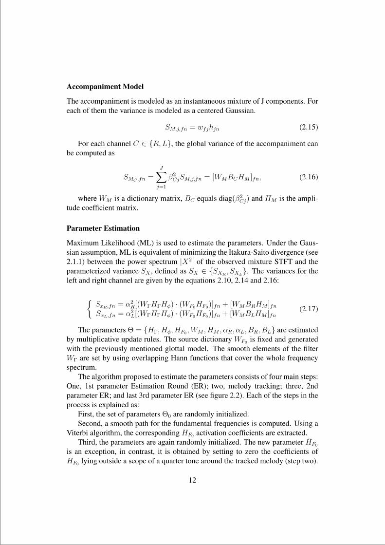
Accompaniment Model

The accompaniment is modeled as an instantaneous mixture of J components. Foreach of them the variance is modeled as a centered Gaussian.

SM,j,fn = wfjhjn (2.15)

For each channel C ∈ {R,L}, the global variance of the accompaniment canbe computed as

SMC ,fn =J∑j=1

β2CjSM,j,fn = [WMBCHM ]fn, (2.16)

where WM is a dictionary matrix, BC equals diag(β2Cj) and HM is the ampli-

tude coefficient matrix.

Parameter Estimation

Maximum Likelihood (ML) is used to estimate the parameters. Under the Gaus-sian assumption, ML is equivalent of minimizing the Itakura-Saito divergence (see2.1.1) between the power spectrum |X2| of the observed mixture STFT and theparameterized variance SX , defined as SX ∈ {SXR

, SXL}. The variances for the

left and right channel are given by the equations 2.10, 2.14 and 2.16:

{SxR,fn = α2

R[(WΓHΓHφ) · (WF0HF0)]fn + [WMBRHM ]fnSxL,fn = α2

L[(WΓHΓHφ) · (WF0HF0)]fn + [WMBLHM ]fn(2.17)

The parameters Θ = {HΓ, Hφ, HF0 ,WM , HM , αR, αL, BR, BL} are estimatedby multiplicative update rules. The source dictionary WF0 is fixed and generatedwith the previously mentioned glottal model. The smooth elements of the filterWΓ are set by using overlapping Hann functions that cover the whole frequencyspectrum.

The algorithm proposed to estimate the parameters consists of four main steps:One, 1st parameter Estimation Round (ER); two, melody tracking; three, 2ndparameter ER; and last 3rd parameter ER (see figure 2.2). Each of the steps in theprocess is explained as:

First, the set of parameters Θ0 are randomly initialized.Second, a smooth path for the fundamental frequencies is computed. Using a

Viterbi algorithm, the corresponding HF0 activation coefficients are extracted.Third, the parameters are again randomly initialized. The new parameter HF0

is an exception, in contrast, it is obtained by setting to zero the coefficients ofHF0 lying outside a scope of a quarter tone around the tracked melody (step two).

12

“thesis” — 2013/9/1 — 14:45 — page 13 — #25

Figure 2.2: Solo/Accompaniment algorithm outline [Durrieu et al., 2009a]

After this second ER round, a first solo/accompaniment separation result V-IMMis obtained (only Voiced parts of the solo are considered).

At last, in the 3rd ER, the initial parameters are the ones estimated in the 2ndER, except for WF0 , where an unvoiced basis vector (uniform value for al thefrequencies) is added. By fixing the filter dictionary Wφ, it is assumed that the un-voiced parts of the solo instrument are generated by the same filters that generatethe voiced parts. By doing this the separation VU-IMM is obtained (voiced andunvoiced parts of the solo are now considered). The multiplicative update rulesfor the parameters can be revised in [Durrieu et al., 2009a].

Source Separation using Wiener Filters

Wiener filters are used to produce an estimate of a target random process by filter-ing another random process through the filter. These filters provide the minimummean square error (MMSE) between the estimated random process and the de-sired process. Thanks to the independence assumption, the frequency response ofthe MMSE estimator obtained with the Wiener filter can be defined as:

GV (f) =SV (f)

SV (f) + SM(f)(2.18)

13

“thesis” — 2013/9/1 — 14:45 — page 14 — #26

For the final separation, with the set of parameters Θ obtained by the algo-rithm, SV and SM are estimated for each frame. Then, following equation 2.18,the corresponding Wiener filter is computed. Finally, applying an overlap-addprocedure, v (i.e., solo track) and m (i.e., accompaniment track) are reconstructed.

2.2.2 Multi-Excitation ModelThe work presented by [Carabias-Orti et al., 2011] and [Rodriguez-Serrano et al., 2012]proposed an approach to model the excitations of musical instruments. Theseexcitations represent vibrating objects, while the filter represents the resonancestructure of the instrument that colors the produced sound. The work focuseson modeling the excitations as the weighted sum of harmonic basis functions,whose parameters are tied across different pitches of an instrument. An NMF-based framework is used to learn the model parameters. As explained in section2.1.1, NMF approaches try to decompose the audio spectrogram of a signal (seein equation 2.8) as a linear combination of spectral basis functions as

xt(f) =N∑n=1

gn,tbn(f) (2.19)

where gn,t is the gain of the basis function n at frame t, and bn(f), n = 1, ..., Nare the bases.

Previous modeling approaches and limitations

As explained in the previous sections, several types of methods have been pro-posed in the literature for estimating this kind of decomposition. Further, it ispossible to constrain the most commonly applied NMF model with some priorssuch as harmonicity, temporal continuity and sparsity.

For instruments in which the partials of each pitch have a smooth distribution,a basic Harmonic Comb (HC) model has turned to be a solution. The elements inthe basis bn,j(f) are approximated by this harmonic shape. The magnitude of theSTFT for the HC model is estimated as

xt(f) =J∑j=1

N∑n=1

gn,t,j

M∑m=1

an,m,jG(f −mf0(n)) (2.20)

where m = 1, ...,M is the number of harmonics, an,m,j the amplitude for them-th partial of the pitch n and instrument j, f0(n) the fundamental frequency ofpitch n, G(f) the magnitude spectrum of the window function and J the number

14

“thesis” — 2013/9/1 — 14:45 — page 15 — #27

of instruments. The parameters that have to be estimated by the NMF algorithmare the time activation coefficients or gains gn,t and the pitch amplitudes an,m,j .

A fundamental problem of this model is that the spectra of certain instruments,like woodwinds or bowed-string instruments, have a specific structure of non-smoothed patterns that varies as a function of the pitch and excitation intensity.For this reason, modeling their spectra as the sum of harmonic elementary func-tions, or using harmonic excitations that are flat as the function of frequency, turnsnot to be sufficient. In order to model the whole pitch range of these instrumentsthe use of more advanced techniques is required.

Excitation or source / filter models, like the ones presented in section 2.2.1 orproposed by [Virtanen and Klapuri, 2006a], try to represent all the possible pitchand instrument combinations, while keeping a reduced amount of parameters. Theexcitation models the time-varying pitch produced by a vibrating element (e.g., apiano string) while the filter models the unique resonant structure of the instrument(e.g., the piano soundboard), which colors the radiated sound.

However, it has been shown that the total admittance of two connected sys-tems, like as a string and a body, is more complex than the product of the ad-mittances of the parts [Woodhouse, 2004]. Therefore, the sound production inthe actual physical system cannot be exactly modeled as the product of an excita-tion and a filter. Though, practical applications of the excitation-filter model haveturned out to be a sufficient approximation.

Harmonic Multi-Excitation Model

As an extension of the previously explained methods, [Carabias-Orti et al., 2011]introduced a new approach that models the excitation as the weighted sum of har-monic excitation basis functions, with parameters as a function of each instrument,and weights that vary as a function of pitch.

For the excitations, it is assumed that a certain instrument should provide anidentifiable characteristic structure. For the filter, the conditions of the musicscene might produce variations in it. Therefore, the excitations of each musicalinstrument and the filter are learned in a training stage. The filter parameters canbe updated in testing to adapt the model to the conditions of the music scene. Theexcitations can be adapted to the variations that the differences between the phys-ical properties of each instrument may introduce.

Excitation: The spectral basis functions of a generic excitation model can berepresented as

bn,j(f) = hj(f)en,j(f). (2.21)

15

“thesis” — 2013/9/1 — 14:45 — page 16 — #28

A generic harmonic excitation is defined as

en,j(f) =M∑m=1

am,n,jG(f −mf0(n)) (2.22)

where am,n,j is the amplitude of the harmonic m, pitch n and instrument j. Theauthor proposes the modeling of the amplitudes as a linear combination of I exci-tation basis vectors vi,m,j as

am,n,j =J∑j=1

wi,n,jvi,m,j (2.23)

where wi,n,j is the weighted sum of the ith excitation basis vector for pitch i andinstrument j. In this case, the excitations are unique for each instrument andpartial but they are shared across pitches. The weights, though, are unique for eachinstrument and pitch but shared between harmonics or partials. By substitutingequation 2.23 into 2.21, we obtain that the harmonic excitation functions can bedefined as

en,j(f) =M∑m=1

I∑i=1

wi,n,jvi,m,jG(f −mf0(n)) (2.24)

Filter: To obtain the spectral basis functions defined in 2.21, the harmonicexcitation functions are multiplied by the instrument filter. The model for a mag-nitude spectrum of the whole signal x(t) is given by the sum of instruments andpitches as

xt(f) =∑n,j

gn,t,jhj(f)M∑m=1

I∑i=1

wi,n,jvi,m,jG(f −mf0(n)) (2.25)

where n = 1, ..., N (with N the number of pitches) and j = 1, ..., J (with Jthe number of instruments), M the number of harmonics and I the number ofconsidered excitations.

The use of a reduced number of excitation bases turns to reduce significantlythe parameters of the model and benefits their learning. This Multi-Excitationmodel is able to produce non-smoothed bases that match better the shape of theoriginal spectrum.

16

“thesis” — 2013/9/1 — 14:45 — page 17 — #29

Parameter estimation

For estimating the parameters of the model an NMF algorithm is proposed. Tominimize the cost function defined in equation 2.4, the Kullback-Leibler diver-gence (see equation 2.6) is used. The multiplicative update rules, which minimizethe divergence, can be revised in [Carabias-Orti et al., 2011]. In practice, as learn-ing the parameters from a polyphonic mixture is a difficult task, recordings with afull pitch range of each instrument (with isolated notes) are provided.

Taking advantage of the temporal gain continuity over gains, an inherent prop-erty in musical instruments, the number of note insertion errors caused by inter-ferences is reduced. For enforcing this temporal continuity of the gains, a Gammachain presented in [Virtanen et al., 2008] is used.

With the presented model, pitch-dependent excitations and instrument-dependentbody responses can be estimated.

2.3 Bowed String Instrument ModelingBowed string instruments are a subcategory of string instruments that are playedby a bow rubbing the strings. Of all the instruments of Western music, the familyof bowed strings is perhaps the most important and most studied. The instrumentsproduced by the Italian masters of the 17th century in Cremona-Amati, Stradivariand others are taken to define the style and quality that modern instruments aimto reproduce.

The bowed string instruments that will be addressed in this work are enclosedinto the violin family and they consist of just four instruments: violin, viola, celloand double bass. More precisely, the case to be addressed consists of a stringquartet, a musical ensemble of four string players, usually composed by two violinplayers, a violist and a cellist. The string quartet is one of the most prominentchamber ensembles in classical music.

2.3.1 Physics and Models of Violin Family InstrumentsFour main basic parts of the violin family instruments can be distinguished: Thestrings, bridge, bow and body.

The strings of a violin are stretched across the bridge and nut of the violin sothat the ends are essentially stationary, allowing for the creation of the mentionedstanding waves. The fundamental frequency and harmonic overtones of the re-sulting sound depend on the material properties of the string, such as the tension,length, mass, elasticity and damping factor.

17

“thesis” — 2013/9/1 — 14:45 — page 18 — #30

The bridge supports one end of the strings playing length and transfers vibra-tion from the strings to the top of the violin. The most significant bridge motionis side-to-side rocking, coming from the transverse component of the strings’ vi-bration.

The bow is generally the one in charge of the excitation of string vibration.It consists of a flat ribbon of parallel hairs stretched between the ends of a stick.They are usually made of wood or synthetic materials, such as fiberglass or carbon-fiber composite. The length, weight, and balance point of modern bows are stan-dardized. The three most prominent factors that the player can control are bowspeed, downward force, and location of the point where it crosses string.

The body of a violin family instrument consists of two arched wooden platesas top and bottom of a box. An internal sound post helps transmit sound to theback of the violin and serves as structural support. It acts as a sound box to couplethe vibration of strings to the surrounding air, making it audible. The constructioncharacteristics of this soundbox have a huge influence in the overall sound qualityof the instrument [Schelleng, 1974].

The core of the violin or any of its relatives (viola, cello, bass) is the bowedstring. The string plays a major role in establishing the musical identity of thisfamily of instruments. Conceptually, the string is the simplest of the compo-nents. However, the action of the string under the bow presents many unan-swered questions. One of the first attempts to understand the phenomena whenstring was bowed was made by Hermann von Helmholtz. With the use of a vi-bration microscope, what we nowadays will name an oscilloscope, he acquiredthe basis for a mathematical description of the motion of the string as a whole[Helmholtz, 1860].

Two simple physical facts underlie the action of the bowed string. First, relieson the fact that the sliding friction is smaller than the static friction and the changefrom one to the other is almost discontinuously abrupt. Second, that the flexiblestring in tension has a succession of natural modes of vibration whose frequen-cies are almost exact whole-number multiples of the lowest frequency. Withoutoutside compulsion, the string is therefore by its very nature given to produce acuasi-periodic sound pressure wave.

According to the models, a linear harmonic model has guided a good deal ofcontemporary violin research [Fletcher, 1999]. The complex frequency envelopethat describes the behavior of the violin body is usually represented by a simpletransfer function. The easiest measurement to interpret is the mechanical admit-tance (velocity to force ratio) at the bridge of the instrument where the string rests.

As seen in Figure 2.3, for the violin, the lowest peak is associated with theair mode coupled in phase with the lowest body mode. Higher resonances areassociated with an out of phase coupling of these two modes and with the direct

18

“thesis” — 2013/9/1 — 14:45 — page 19 — #31

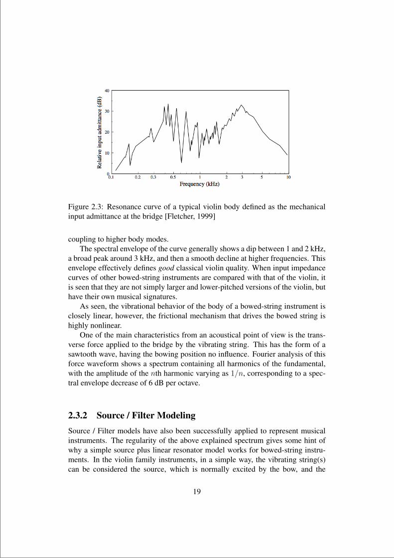
Figure 2.3: Resonance curve of a typical violin body defined as the mechanicalinput admittance at the bridge [Fletcher, 1999]

coupling to higher body modes.The spectral envelope of the curve generally shows a dip between 1 and 2 kHz,

a broad peak around 3 kHz, and then a smooth decline at higher frequencies. Thisenvelope effectively defines good classical violin quality. When input impedancecurves of other bowed-string instruments are compared with that of the violin, itis seen that they are not simply larger and lower-pitched versions of the violin, buthave their own musical signatures.

As seen, the vibrational behavior of the body of a bowed-string instrument isclosely linear, however, the frictional mechanism that drives the bowed string ishighly nonlinear.

One of the main characteristics from an acoustical point of view is the trans-verse force applied to the bridge by the vibrating string. This has the form of asawtooth wave, having the bowing position no influence. Fourier analysis of thisforce waveform shows a spectrum containing all harmonics of the fundamental,with the amplitude of the nth harmonic varying as 1/n, corresponding to a spec-tral envelope decrease of 6 dB per octave.

2.3.2 Source / Filter ModelingSource / Filter models have also been successfully applied to represent musicalinstruments. The regularity of the above explained spectrum gives some hint ofwhy a simple source plus linear resonator model works for bowed-string instru-ments. In the violin family instruments, in a simple way, the vibrating string(s)can be considered the source, which is normally excited by the bow, and the

19

“thesis” — 2013/9/1 — 14:45 — page 20 — #32

sound box together with the bridge can be approached as the filter. The gener-alized model proposed by [Hahn et al., 2010] is also applied for the violin. Thesource-filter-model aims to represent the time-varying spectral characteristics ofquasi-harmonic instruments. For this, it is composed of an excitation source, gen-erating sinusoidal parameter trajectories, and a modeling resonance filter, whereasbasic-splines are used to model continuous trajectories.

The work by [Virtanen and Klapuri, 2006b] proposes a method where the in-put spectrogram of polyphonic audio is modeled as a linear sum of basis functionswith time-varying gains. Each of the basis is represented as a product of a sourcespectrum and the magnitude response of a filter. This modeling can also be foundin the source separation literature for the specific case of performing musical in-strument recognition [Heittola et al., 2009]. In this approach, the mixture signal isdecomposed by NMF and modeled as a product of excitations and filters. The ex-citations are restricted to harmonic spectra and their fundamental frequencies areestimated in advance using a multipitch estimator, whereas the filters are restrictedto have smooth frequency responses by modeling them as a sum of elementaryfunctions. More precisely, the filter consists of elementary triangular bandpassmagnitude responses, uniformly distributed on the Mel-frequency scale.

This previous works show that source-filter models outperform the standardNMF representations for singing voice signals and polyphonic audio. One of theadvantages of this formulation is the reduction the number of free parametersneeded to approximate the audio signals, which leads to a more reliable parameterestimation.

20

“thesis” — 2013/9/1 — 14:45 — page 21 — #33

Chapter 3

METHODOLOGY

After understanding and acknowledging the advantages and limitations of currentstate of the art algorithms in source separation, our hypothesis is that it is possibleto provide external information, such as the melodies or timbral characteristicsof each of the instruments, in order to enhance their results. Such steps will beinvestigated following the methodology presented in this chapter.

First, the initial approach and the modifications of the previously explainedInstantaneous Mixture Model (IMM) are explained. Second, the Multi-excitationModel and the proposed modifications are exposed. In here, both the modifica-tions to the source and the filter representations are introduced.

3.1 First approach: Modifications over the IMMHaving the previously presented Instantaneous Mixture Model as a starting point(see Section 2.2.1), some modifications to match our requirements have been in-troduced. The original model is designed to separate a single predominant or leadinstrument, being explicitly focused on the singing voice. In contrast, we mainlywant to perform the separation of bowed-string instruments.

3.1.1 Source ModelExcitation bases

The source variance of the model is parameterized as a combination of its basesWF0 and the time-varying activation coefficients HF0 as expressed in equation2.14. Since it is mainly focused on separating the singing voice, the bases ofthe source are defined by a previously exposed KLGLOT88 glottal source model.Specifically, it is modeled as a non-negative linear combination of the spectralcombs of all the NF0 possible (allowed) fundamental frequencies. An example of

21

“thesis” — 2013/9/1 — 14:45 — page 22 — #34

Figure 3.1: Example of an WF0 basis generated with the glottal source model

a generated spectral comb base of the glottal source can be seen in figure 3.1. Aswe want the excitation bases to be able to fit other instruments, and not only thesinging voice, the excitations are modified to follow a flat pattern. That is, a po-tentially more flexible and less restrictive solution is chosen. The new source ex-citation bases are described by impulse trains that cover the allowed F0 frequencyrange. The excitations are restricted to harmonic spectra and their fundamentalfrequencies are obtained as follows.

Excitation gains

In order to obtain the HF0 gains or activation coefficients, the model estimates themain melody over the mixture. As it will be explained later, our proposed modelaims to separate as many instrument as are present in the mixture, not only thepredominant or lead one. Following the procedure of the original model involvesthe estimation off all the fundamental frequencies of the various instruments overthe mixture. In order to skip the difficulties that actual multipitch estimation al-gorithms entail, the pitch or fundamental frequency estimation of each of the in-struments present in the mixture is provided to the system. That is, as a firstmodification, the fundamental frequency estimation step is avoided. Instead, itis obtained from prior information and later provided to the system. As we haveexposed, this approach is known in the literature as Informed Source Separation,since more information than the audio mixture is provided to the system.

22

“thesis” — 2013/9/1 — 14:45 — page 23 — #35

Figure 3.2: Source / filter + accompaniment diagram of the modified IMM

To obtain this prior knowledge, different information like the musical score,isolated pick-up recordings or even the multitrack recordings have to be avail-able. Musical score following and audio alignment is a broad topic of researchand is not intended to be covered in this work. In order to more simply obtainthe required data to inform the separation and focus on developing other aspectsof the model, the pitch information is directly estimated from individual instru-ment recordings. The nature of this recordings can be different. Thanks to theavailability of multimodal datasets, they are recently more and more accessible.On the one hand, by means of pick-up piezoelectric microphones located in thebody of the instruments, the clean vibrations that the sound produces are directlycaptured. Pitch estimation over this signals is simpler to perform than from thecomplex mixture, where more instruments are present too. The obtained signalsprovide a clean representation of the melody being played. On the other hand,when multitrack recordings are available, the pitch estimation can be directly per-formed from this recordings. A pitch estimation algorithm will perform better inthis isolated monophonic recordings than in the complex polyphonic mixture. Asopposed to the musical score, the fundamental frequency obtained from this sig-nals is more complete, since it contains information that it’s not usually present inthe former, such as vibratos. Besides, the melody lines are obtained directly fromthe aligned audio, so there is no need of performing any other alignment process.

More precisely, we use Yin [De Cheveigne and Kawahara, 2002], a state-of-the-art predominant f0 estimation algorithm, over this isolated recordings to ob-tain the prior melodic information. Finally, the source / filter model is providedwith the fundamental frequency of the lead instrument (see figure 3.2). Thanksto the obtained pitch information, the HF0 gains of the source are fixed. In thismanner, the gains are not longer estimated in the separation process.

Summing up, the excitations are restricted to harmonic spectra and their fun-damental frequencies are obtained in a prior step to the separation. When combin-

23

“thesis” — 2013/9/1 — 14:45 — page 24 — #36

ing both WF0 bases and HF0 activations the source variance SF0 is obtained. Thissource can be interpreted as the different pitch values (notes) of the instrument tobe separated.

3.2 Proposed Extensions: Combining IMM and Multi-Excitation Model

As mentioned before, one of the goals of the system is to be able to separate asmany instruments as present in the audio mixture. However, the original proposalof the IMM is limited to separate only the predominant instrument. To allow thefull separation of the mixture, the IMM has been extended with two modificationsinspired on the Multi-Excitation model (see Section 2.2.2). First, each of theinstruments source is modeled individually. Second, each of the instruments has asource and a filter model assigned to it. The extensions to the model are explainedbellow.

3.2.1 Multi-Excitation and Single Filter IMMBesides keeping the sources flat, a modification that adds one excitation for eachof the instruments present in the mixture is introduced. With this extension, themodel assigns now as many sources as instruments are present in the mixture.More specifically, the model generates a source for each of the different funda-mental frequency or melody lines provided. The filter sub-model is shared amongall the sources.

In the case where prior information to estimate the pitch of one or more of theinstruments is not available, the separation of this instrument is not performed.The decomposition of this instrument or instruments is not done with the source /filter model, but it is represented by the general NMF accompaniment sub-model.In other words, if the pitches of all the four instruments of a string quartet areestimated in a previous step and provided to the system, all of the four instrumentsare separated. However, lets assume that from a mixture of four instruments onlythe pitch information of two of them, e.g. the cello and the viola, is provided.Each of this instruments is assigned with its own source model and the other two,in this case both violins, are fitted into the accompaniment sub-model.

The source variance previously defined by equation 2.12 can be redefined forthis extension as

SF0 =

NI∑i

SiF0=

NI∑i

W iF0H iF0

(3.1)

24

“thesis” — 2013/9/1 — 14:45 — page 25 — #37

where SiF0is now the source variance of instrument i. Each of the instruments

provided pitch i is assigned to H iF0

. The bases W iF0

are generated according to theestimated fundamental frequencies.

Having this modification in the source into account, the global variance can beredefined now as

VmesfIMM =

NI∑i

((W iF0H iF0

) · (WΓHΓHφ)) +WMHM (3.2)

The update rules for the parameter estimation of this method remain the sameas for the specified for the IMM (see Section 2.2.1). In contrast, for this new casethe parameters to be updated are increased, since the H i

F0matrix is different for

each source.According to the filter model, even if one excitation for each of the instru-

ments is now defined, only one filter for all of them is assigned. Since this modelis derived by combining the IMM and the Multi-Excitation models, it will be ad-dressed as the Multi-Excitation and Single Filter IMM. A general diagram of thenew proposed model can be seen in figure 3.3.

Figure 3.3: Multi-Excitation and Single Filter IMM diagram

3.2.2 Multi-Excitation and Multi-Filter IMMAs a second step, the filter model is extended to have multiple source and filtermodels. This proposed model assigns one specific filter to each instrument exci-tation.

Each of the instruments is modeled now with its own excitation and filter. Forthis reason, the filter bases and activations have to be estimated for each of theinstruments too. The filter variance previously defined by equation 2.13 can beredefined for this extension as

25

“thesis” — 2013/9/1 — 14:45 — page 26 — #38

Sφ =

NI∑i

Siφ =

NI∑i

W iφH

iφ =

NI∑i

WΓHiΓH

iφ (3.3)

where SiF0is now the source variance of instrument i. The WΓ,H i

Γ and H iφ

matrices are different for each source.With the filter sub-model extension, the global variance can be redefined now

as

VmefIMM =

NI∑i

((W iF0H iF0

) · (WΓHiΓH

iφ)) +WMHM (3.4)

The update rules for the parameter estimation of this method remain the sameas for the specified for the IMM (see Section 2.2.1). In contrast, as in the previousextension, the parameters to be updated are increased. As mentioned, the H i

Γ, H iφ

and H iF0

matrices are different for each source sound. Each of the instrumentsprovided pitch i is assigned to H i

F0and its bases W i

F0are generated accordingly.

When a target source is estimated from the mixture spectrogram only the activa-tions H i

Γ, H iφ and H i

F0of the corresponding pitch are used.

Figure 3.4: Multi-Excitation and Multi-Filter IMM diagram

Summing up, one excitation and one filter for each of the instruments is nowassigned. Since this model is derived by combining the IMM, Multi-Excitationmodel and a multiple filter model, it will be addressed as the Multi-Excitation andMulti-Filter IMM. An overview of the new proposed model can be seen in figure3.4.

26

“thesis” — 2013/9/1 — 14:45 — page 27 — #39

3.3 Supervised Timbre ModelsIn order to reduce the amount of parameters to be estimated and to facilitate theseparation, a new method to obtain the filter bases from a previous training processis proposed. The prior training of different filter bases that represent the timbrecharacteristics of each instrument is here introduced.

The filter sub-model is specified in equation 2.13 and redefined for the pro-posed Multi-Excitation and Multi-Filter IMM in equation 3.3. A decompositionof the Wφ bases in two other matrixes is introduced (see figure 3.5). The smoothfilter dictionaryW i

φ is originally defined in the IMM as part of a production modelfor instrument i. Applying it to the Multiple-Excitation and Filter IMM, this basesare explained as a new combination of smooth filter bases WΓ and its activationsH i

Γ for each instrument i. The smoothness of the filters is more realistic thanhaving unconstrained filters. Rather than a direct improvement in the source sepa-ration, this decomposition allows to learn the spectral shapes that are characteristicfor a given instrument in this proposed supervised framework.

Figure 3.5: Timber model Wφ bases decomposed into an smooth filter dictionarybases WΓ and its gains HΓ.

The WΓ smooth filters are fixed for all the instruments, they are composed byoverlapping Hann functions covering the whole frequency range. Only the desirednumber of smooth filters has to be provided to the system, a parameter that can beconsidered an equivalent to the frequency resolution of the filter representation.When more filters are defined, the spectral shape or timbre can be more preciselyrepresented.

To obtain each of the different instrument filter models a recording where onlyaudio content of this specific instrument has to be provided. Over this data, thefilter smooth dictionary bases WΓ are generated, whereas the filter dictionary ac-tivations H i

Γ are estimated and saved. This way, the combination of both basesand activations result in some bases (timbre bases) that can bee seen as a model

27

“thesis” — 2013/9/1 — 14:45 — page 28 — #40

containing the timbre characteristics of the instrument in the provided data. Ex-amples of the different generated and estimated matrices can be seen in Figures3.6 and 3.7.

Figure 3.6: Timbre matrices example over a cello excerpt. Smooth filter dictionarybases WΓ (top), its activations HΓ (middle) and the obtained bases Wφ

The obtained timbre model is now used in the separation process. When sep-arating the sources of a mixture where a certain instrument i is present, the previ-ously created model of this instrument i can be loaded into the system. The WΓ

bases are again generated. The H iΓ activations are loaded from the i instrument

timbre model. Both matrices create the smooth filter dictionary W iφ that is kept

fixed during the separation. However, the Hφ activations of this dictionary, sincethey are still depend of the content of the mixture, have to be still estimated.

According to the update rules, the parameter estimation of this method remainsthe same as for the proposed Multi-Excitation and Filter IMM (see Section 3.2.2).However, as theH i

Γ are loaded from the previously supervised timbre models theydon’t have to be estimated and are kept fixed through the process.

In other words, one excitation and one filter for each of the instruments isassigned. In the filter part, a previously supervised timbre model is provided for

28

“thesis” — 2013/9/1 — 14:45 — page 29 — #41

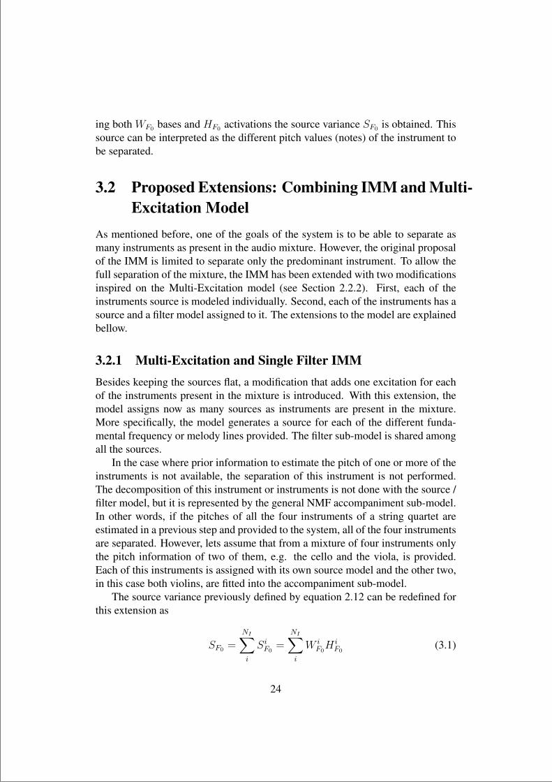
Figure 3.7: Timbre matrices example over a violin excerpt. Smooth filter dictio-nary bases WΓ (top), its activations HΓ (middle) and the obtained bases Wφ

each instrument. Figure 3.8 shows a general diagram of the Multi-Excitation andMulti-Filter IMM where the supervised filters are loaded.

Figure 3.8: Multi-Excitation and Multi-Filter IMM diagram with supervised filtersloaded

29

“thesis” — 2013/9/1 — 14:45 — page 30 — #42

Chapter 4

EVALUATION AND RESULTS

4.1 Evaluation MetricsAn intuitive way to assess the quality of a source separation algorithm could be tolisten to the extracted sounds and to evaluate them with our own subjective crite-ria. However, in order to obtain more general results and to allow an fair compar-ison between different methods, we need to compute some objective evaluationmeasures. Different approaches have been proposed to calculate these evaluationmetrics, all based on the comparison of the extracted sources with the originalones. The advantage of these evaluation techniques is to be completely impartialand to provide interpretable results. Their inconvenient side is that they require theoriginal separated sources of the signals we intend to separate. Even if multitrackrecordings are more and more available nowadays, the data usable for experimentsis still dramatically reduced.

4.1.1 The BSS EVAL ToolboxThe BSS EVAL toolbox [C.Fevotte et al., 2005], which stands for Blind SourceSeparation Evaluation, allows to compute objective performance measures. Thismetrics are the ones created and proposed by the Signal Separation EvaluationCampaign (SiSEC) 1, a scientific evaluation contest where speech and music datasetsare evaluated and standardized. This metrics evaluate the performance of the sep-aration i.e. how well the estimated sources sj are approximated to the given truesources sj [Vincent et al., 2007]. The estimated sources are decomposed as

sj = starget + einterf + enoise + eartif (4.1)

1http://sisec.wiki.irisa.fr/

30

http://sisec.wiki.irisa.fr/

“thesis” — 2013/9/1 — 14:45 — page 31 — #43

The starget = q(sj) is a modified version of sj with an allowed distortion q thatrepresents the part of sj coming from the target source sj . The einterf, enoise, eartif

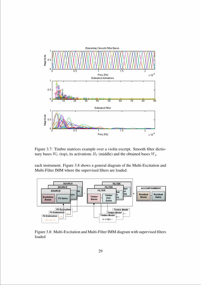
are the interferences, noise and artifacts error terms that represent the parts of sjcoming from the unwanted sources, from sensor noises and from other artifacts,respectively. The performance metrics are defined as energy ratios (in dB). Threemain metrics are defined.

• Source to Distortion Ratio:

SDR = 10log10

‖starget‖2

‖sj − starget‖2 (4.2)

• Source to Interference Ratio, which considers sounds from other sources:

SIR = 10log10

‖starget‖2

‖einterf‖2 (4.3)

• Source to Artifacts Ratio, related to the artifacts produced by the separation:

SAR = 10log10‖sj − eartif‖2

‖eartif‖2 (4.4)

The three performance measurement tools defined in this toolbox are inspiredin the traditional measure of Signal to Noise Ratio (SNR), thus, the interpretationof the metrics is not complex.

4.1.2 The PEASS ToolkitA further possibility is to use the Perceptual Evaluation methods for Audio SourceSeparation (PEASS) toolkit as proposed by [Emiya et al., 2011]. This softwareallows the computation of objective measures to assess the perceived quality ofestimated source signals, based on perceptual similarity measures obtained withthe PEMO-Q auditory model [Huber and Kollmeier, 2006]. For this approach, theestimated sources sj are decomposed in a similar manner to 4.1 as

sj − sj = starget + einterf + eartif (4.5)

In here, the terms einterf, enoise, eartif the target distortion, the interference andthe artifacts components, respectively.

In order to provide, in addition to the classic energy ratios, perceptually moti-vated results the following new performance metrics are introduced:

31

“thesis” — 2013/9/1 — 14:45 — page 32 — #44

• Overall Perceptual Score (OPS)

• Target-related Perceptual Score (TPS)

• Interference-related Perceptual Score (APS)

• Artifacts-related Perceptual Score (APS)

Using the perceptual similarity measure (PSM) provided by the PEMO-Q au-ditory model, the scores are obtained by measuring the salience of each distor-tion component individually. To do so, the estimated sources are compared withthemselves and the considered distortions are subtracted. The following saliencefeatures are obtained

qjoverall = PSM(sj, sj) (4.6)

qjtarget = PSM(sj, sj − starget) (4.7)

qjinterf = PSM(sj, sj − einterf) (4.8)

qjartif = PSM(sj, sj − eartif) (4.9)

A nonlinear mapping is applied to these salience features, combine these fea-tures into a single scalar measure for each grading task and to adapt the featurescale to the subjective grading scale. In addition to the classic energy ratios (indB), this method allows to provide the perceptual scores presented above (in %).

4.2 Description of the DatasetIn order to perform a Since the available datasets with score-aligned tracks or mul-titrack recordings are very few, [Fritsch, 2012] introduced a new dataset namedTRIOS. The dataset is formed by five short extracts from chamber music triopieces. Besides the mixtures, each separated instrumental track is provided. Sinceour interest is mainly to focus on bowed-string instruments, only two of the fiverecordings are used:

• a trio for violin, cello and piano by Franz Schubert (D.929, op.100)

• a trio for viola, clarinet and piano by Wolfgang Amadeus Mozart (K.498)

The database is accessible in the C4DM Research Data Repository2. Moredetails about the dataset can be found in [Fritsch, 2012].

2http://c4dm.eecs.qmul.ac.uk/rdr/handle/123456789/27

32

“thesis” — 2013/9/1 — 14:45 — page 33 — #45

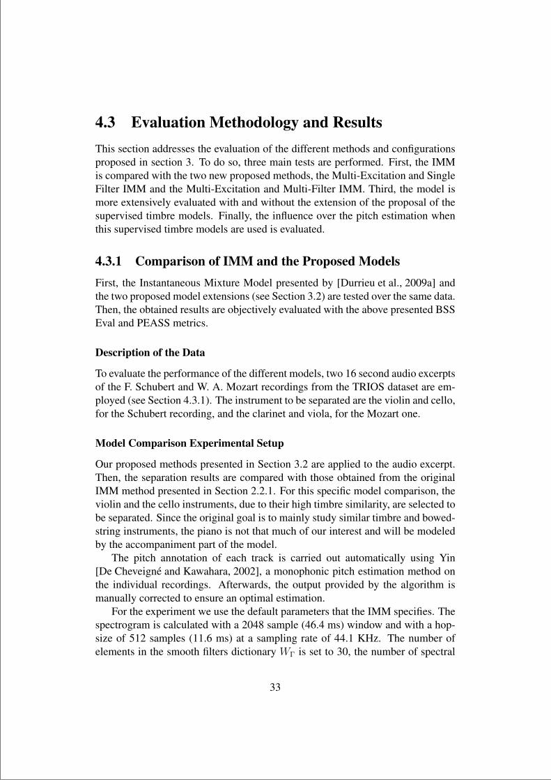
4.3 Evaluation Methodology and ResultsThis section addresses the evaluation of the different methods and configurationsproposed in section 3. To do so, three main tests are performed. First, the IMMis compared with the two new proposed methods, the Multi-Excitation and SingleFilter IMM and the Multi-Excitation and Multi-Filter IMM. Third, the model ismore extensively evaluated with and without the extension of the proposal of thesupervised timbre models. Finally, the influence over the pitch estimation whenthis supervised timbre models are used is evaluated.

4.3.1 Comparison of IMM and the Proposed ModelsFirst, the Instantaneous Mixture Model presented by [Durrieu et al., 2009a] andthe two proposed model extensions (see Section 3.2) are tested over the same data.Then, the obtained results are objectively evaluated with the above presented BSSEval and PEASS metrics.

Description of the Data

To evaluate the performance of the different models, two 16 second audio excerptsof the F. Schubert and W. A. Mozart recordings from the TRIOS dataset are em-ployed (see Section 4.3.1). The instrument to be separated are the violin and cello,for the Schubert recording, and the clarinet and viola, for the Mozart one.

Model Comparison Experimental Setup

Our proposed methods presented in Section 3.2 are applied to the audio excerpt.Then, the separation results are compared with those obtained from the originalIMM method presented in Section 2.2.1. For this specific model comparison, theviolin and the cello instruments, due to their high timbre similarity, are selected tobe separated. Since the original goal is to mainly study similar timbre and bowed-string instruments, the piano is not that much of our interest and will be modeledby the accompaniment part of the model.

The pitch annotation of each track is carried out automatically using Yin[De Cheveigne and Kawahara, 2002], a monophonic pitch estimation method onthe individual recordings. Afterwards, the output provided by the algorithm ismanually corrected to ensure an optimal estimation.

For the experiment we use the default parameters that the IMM specifies. Thespectrogram is calculated with a 2048 sample (46.4 ms) window and with a hop-size of 512 samples (11.6 ms) at a sampling rate of 44.1 KHz. The number ofelements in the smooth filters dictionary WΓ is set to 30, the number of spectral

33

“thesis” — 2013/9/1 — 14:45 — page 34 — #46

shapes for the filter part is set to 10, the number of elements for the accompani-ment is 40 and the number of iterations 30.

It has to be mentioned that as two instruments are being separated, the originalIMM has to be performed twice. First, providing the melody of the violin andsecond, providing the one of the cello. In contrast, since the proposed models areable to separate as many instrument as wanted, there is no need of performing theprocess twice.

Results

The results are objectively evaluated with the metrics specified in BSS Eval andPEASS toolkits.

First, the SDR, SIR and SAR scores for the Schubert audio excerpt are pre-sented in Tables 4.1, 4.2 and 4.3, respectively.

IMM MESF IMM MEF IMM violin 4,0278 6,2247 5,7874

cello -‐16,6330 6,0827 6,6009

average -‐6,3026 6,1537 6,1942

-‐20,0 -‐15,0 -‐10,0 -‐5,0 0,0 5,0 10,0

SDR (dB)

Table 4.1: SDR score results by model for the Schubert audio excerpt


cello 5,4401 13,6190 16,0080

average 10,0021 12,9640 14,1020

0,0 2,0 4,0 6,0 8,0 10,0 12,0 14,0 16,0 18,0

SIR (dB)

Table 4.2: SIR score results by model for the Schubert audio excerpt

34

“thesis” — 2013/9/1 — 14:45 — page 35 — #47


cello -‐15,5140 7,1101 7,2372

average -‐5,4676 7,4056 7,2031

-‐20,0

-‐15,0

-‐10,0

-‐5,0

0,0

5,0

10,0

SAR (dB)

Table 4.3: SAR score results by model for the Schubert audio excerpt

Second, the SDR, SIR and SAR scores for the Mozart audio excerpt are pre-sented in Tables 4.1, 4.2 and 4.3, respectively.

IMM MESF IMM MEF IMM clarinet -‐3,0966 12,3680 12,4920

viola 2,3204 0,3056 3,0215

average -‐0,3881 6,3368 7,7568

-‐4,0 -‐2,0 0,0 2,0 4,0 6,0 8,0 10,0 12,0 14,0

SDR (dB)

Table 4.4: SDR score results by model for the Mozart audio excerpt

IMM MESF IMM MEF IMM clarinet 16,2340 19,7250 19,9770

viola 3,1250 7,7636 10,0260

average 9,6795 13,7443 15,0015

0,0

5,0

10,0

15,0

20,0

25,0

SIR (dB)

Table 4.5: SIR score results by model for the Mozart audio excerpt

35

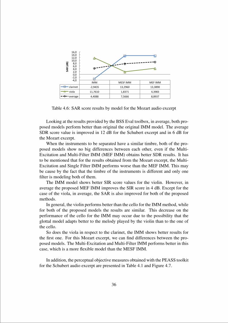
“thesis” — 2013/9/1 — 14:45 — page 36 — #48

IMM MESF IMM MEF IMM clarinet -‐2,9435 13,2960 13,3890

viola 11,7610 1,8371 4,3983

average 4,4088 7,5666 8,8937

-‐4,0 -‐2,0 0,0 2,0 4,0 6,0 8,0 10,0 12,0 14,0 16,0

SAR (dB)

Table 4.6: SAR score results by model for the Mozart audio excerpt

Looking at the results provided by the BSS Eval toolbox, in average, both pro-posed models perform better than original the original IMM model. The averageSDR score value is improved in 12 dB for the Schubert excerpt and in 6 dB forthe Mozart excerpt.

When the instruments to be separated have a similar timbre, both of the pro-posed models show no big differences between each other, even if the Multi-Excitation and Multi-Filter IMM (MEF IMM) obtains better SDR results. It hasto be mentioned that for the results obtained from the Mozart excerpt, the Multi-Excitation and Single Filter IMM performs worse than the MEF IMM. This maybe cause by the fact that the timbre of the instruments is different and only onefilter is modeling both of them.

The IMM model shows better SIR score values for the violin. However, inaverage the proposed MEF IMM improves the SIR score in 4 dB. Except for thecase of the viola, in average, the SAR is also improved for both of the proposedmethods.

In general, the violin performs better than the cello for the IMM method, whilefor both of the proposed models the results are similar. This decrease on theperformance of the cello for the IMM may occur due to the possibility that theglottal model adapts better to the melody played by the violin than to the one ofthe cello.

So does the viola in respect to the clarinet, the IMM shows better results forthe first one. For this Mozart excerpt, we can find differences between the pro-posed models. The Multi-Excitation and Multi-Filter IMM performs better in thiscase, which is a more flexible model than the MESF IMM.

In addition, the perceptual objective measures obtained with the PEASS toolkitfor the Schubert audio excerpt are presented in Table 4.1 and Figure 4.7.

36

“thesis” — 2013/9/1 — 14:45 — page 37 — #49

Figure 4.1: Overall Perceptual Score (OPS) results by model for the Schubertaudio excerpt

!"#$%!"# $"# %"# &"# !"# $"# %"# &"# !"# $"# %"# &"#

'()*(+ ,-./0 1.2/ 32.31 -1.4, ,0.,, 23./2 /4./4 2,.24 ,5.-1 2,.44 /4.4/ 2/.-367**) 1.// 8.41 -8.22 -3.-4 -8.-, -.-0 0.32 ,2.-8 1.81 -.-0 3.-2 ,/.-1

&'$(&)$ -3./3 3.80 2-.10 -4./3 -5.-4 -5.,1 ,4.88 ,4.4/ -5.0/ -0.10 ,0./2 ,1.-4

!"#$%&!! !"$%&!!&!!

Table 4.7: PEASS toolkit results by model for the Schubert audio excerpt

The perceptual objective measures obtained with the PEASS toolkit for theMozart audio excerpt are exposed in Table 4.2 and Figure 4.8.

Figure 4.2: Overall Perceptual Score (OPS) results by model for the Mozart audioexcerpt

37

“thesis” — 2013/9/1 — 14:45 — page 38 — #50

!"#$%!"# $"# %"# &"# !"# $"# %"# &"# !"# $"# %"# &"#

'()*+,-. /01/2 0132 331/2 4132 43152 3612/ 37163 36125 44175 381/8 37107 39185:+;() /0155 0127 8140 /4192 /7175 /127 6180 /9163 //137 /147 7130 //129

&'$(&)$ /0146 0195 79163 2152 74137 7312/ 75147 47178 77144 75175 7717/ 78130

!"#$%&!! !"$%&!!&!!

Table 4.8: PEASS toolkit results by model for the Mozart audio excerpt

As Figures 4.1 and 4.2 depict, the Overall Perceptual Score (OPS) obtained bythe IMM is improved by both of the proposed MESF IMM and MEF IMM. As itcan be seen from the results of both recordings, when the instruments have a moresimilar timbre (violin and cello, Schubert), the improvement over the OPS is notas high as when the instruments have a more different timbre (clarinet and viola,Mozart).

4.3.2 Multi-Excitation and Multi-Filter Model Parameter Op-timization

During the many experiments that have been run through the design of the pro-posed method, it has been observed that the separation results may vary dependingon the various parameters of the general decomposition process. The parametersthat describe the decomposition, i.e. the number of bases of the filter dictionary,seem to be influential over the results.

Thus, before comparing the model with the supervised timbre models exten-sion, a parameter optimization grid-search is performed. The goal of this searchis no other than to obtain the best possible combination of parameters to representthe filter sub-model.


The previously presented TRIOS dataset (see Section 4.3.1) is also used to evalu-ate this model and the timbre filters.

For the filter sub-model parameter optimization, the same 16 second extractemployed in the previous model comparison test of the F. Schubert recording isused.

Parameter Optimization Experimental Setup

In order to obtain the best parameter configuration, a grid-search is performedover the audio excerpt. The violin and the cello instruments are the ones to beseparated. The pitch is extracted over the recording as explained in Section 4.3.1.

38

“thesis” — 2013/9/1 — 14:45 — page 39 — #51

The piano is not modeled and is approximated by the accompaniment. The goalof this test is to find how the different parameters values are influential for the sep-aration and which ones are the more convenient for our scenario. The parametersand values tested are the following:

• P smooth elementary filters of the WΓ dictionary: 10, 30, 70, 90, 100 and120.

• K filters to be considered (bases): 1, 2, 3, 10, 20 and 30.

• Iterations: 10, 30, 50, 70 and 90.

Results

The results are evaluated with the objective metrics specified in BSS Eval toolbox.The SDR score is the measure that has been taken as the main reference to judgethe best results.

10iter 30iter 50iter 70iter 90iter violin 5,5673 7,3023 6,4457 7,1337 7,1651

cello 6,2863 7,3423 5,7395 5,0415 5,7294

accompaniment 7,6324 8,6341 6,8046 6,3999 6,0596

average 6,4953 7,7596 6,3299 6,1917 6,3180

1,0 2,0 3,0 4,0 5,0 6,0 7,0 8,0 9,0 10,0

SDR (dB)

Table 4.9: SDR score results by iteration over 90 P smooth filters and 20 K bases

39

“thesis” — 2013/9/1 — 14:45 — page 40 — #52

P10 P30 P70 P90 P100 P120 violin 5,8796 6,3414 7,1159 7,3023 7,1923 6,6956

cello 6,5791 6,5270 6,7922 7,3423 7,2596 6,8402

accompaniment 7,1346 7,3252 7,8744 8,6341 8,3647 7,8615

average 6,5311 6,7312 7,2608 7,7596 7,6055 7,1324

5,0 5,5 6,0 6,5 7,0 7,5 8,0 8,5 9,0

SDR (dB)

Table 4.10: SDR score results by P smooth filters over 30 iterations and 20 Kbases

K1 K2 K3 K10 K20 K30 violin 5,8473 6,3531 6,2651 7,1837 7,3023 7,1899

cello 5,7825 6,6088 6,9065 7,3907 7,3423 6,9473

accompaniment 6,9177 7,6831 7,5616 8,5001 8,6341 8,3546

average 6,1825 6,8817 6,9111 7,6915 7,7596 7,4973

5,0 5,5 6,0 6,5 7,0 7,5 8,0 8,5 9,0

SDR (dB)

Table 4.11: SDR score results by K bases over 90 P smooth filters and 30 itera-tions

!"#$%&'$#()* !"*+(($,"-#.$%&* ""/'*%*01 21 31

Table 4.12: Best parameter configuration over different tested K bases, P smoothfilters and iterations values

As shown in Tables 4.9, 4.10, 4.11 and 4.12 the best SDR results are obtainedfor 90 P smooth elementary filters of the WΓ dictionary, 20 K number of filtersand 30 iterations. When running the estimation over more iterations, the estima-tion error keeps decreasing. However, since the SDR decreases, there must beleakage from one source to another, having a worse separation quality.

The complete table of results can be found in Appendix A.

40

“thesis” — 2013/9/1 — 14:45 — page 41 — #53

4.3.3 Multi-Excitation and Multi-Filter Model with SupervisedTimbre Model Extension

The second test consist of comparing the performance of the proposed Multi-Excitation and Multi-Filter model when the filters are estimated over the mixtureand the performance when the supervised timbre models are loaded to the filters(see Sections 3.3 and 3.2.2, respectively).


The previously presented TRIOS dataset is also used to evaluate this model andthe timbre filters (see Section 4.3.1).

For the comparison between the proposed Multi-Excitation and Multi-Filtermodel and the extension with the supervised timbre models, both F. Schubert andW. A. Mozart recordings are used. The entire duration of the recordings is nowconsidered for this test.

For the different pitch estimations test, two new mixes of instruments are cre-ated. The violin and the cello from F. Schubert recording are combined in a newmixture. The clarinet and viola from the W. A. Mozart recording are joined in anew mixture too. The piano is not included in any of the new mixtures.

Supervised Timbre Model Performance Experimental Setup

The performance of the Supervised Timbre Models is evaluated in three differentexperiments.

- Performance of the Timbre Models:

The first part of this test consist of comparing the performance of the proposedMulti-Excitation and Multi-Filter model when the filters are estimated over themixture and when the supervised timbre models are loaded into the model. Anextra case where the filters are unsupervised, this is, randomly initialized, and notupdated is also introduced. This case will theoretically provide a bottom line orworst-case scenario for the filter sub-model.

In order not to train and test the filters with exactly the same data a N-FoldCross Validation is performed. The number of folds is determined by the durationof the recordings and the folds themselves. In other words, it is a compromisebetween not letting the amount of information provided to the system be an in-fluence over the performance of the model, and having enough different folds totrain the timbre models and test it over the recording. Thus, each fold is selectedto have a minimum amount of data of approximately 8.5 seconds. The influenceof this parameter, which is referred in this work as block size, is tested afterwards.

41

“thesis” — 2013/9/1 — 14:45 — page 42 — #54

For the above mentioned F. Schubert recording from the TRIOS dataset, theaudio is divided into 6 folds. Each of the test audio extracts has an approximateduration of 8.5 seconds. Each of the training audio extracts, in contrary, an ap-proximate of 45 seconds.

For the W. A. Mozart recording, since the length of the recording is shorterthan the former, the audio is divided into 4 folds. Each of the test audio extractshas an approximate duration of 8.5 seconds. Each of the training audio extracts,in contrary, an approximate of 26 seconds.

The configuration for this test is obtained from the results of the parameteroptimization test explained in Section 4.3.2. This is, the number of P smoothelementary filters of the WΓ dictionary is set to 90, the K number of filters to beconsidered is 20 and the number of iterations is 30.

Results

The results are evaluated with the objective metrics specified in BSS Eval toolbox.

!"#$%!"# !$# !%# !"# !$# !%# !"# !$# !%#

&'()'* +,-. /.,01 2,32 .,20 /4,+- +,4. 5/.,/- 0,/+ .,0167))( .,-2 /3,/+ +,32 .,-0 /3,+3 8,8/ 53-,22 2,-. 5/2,8+966(:;< .,04 2,-0 //,10 .,03 2,28 /-,01 5+,+2 -,84 11,2+&'$(&)$ .,+2 /3,0+ 2,.4 .,0/ /3,01 +,2- 5/0,11 0,-- .,2/

!"#$%!"# !$# !%# !"# !$# !%# !"# !$# !%#

6)9='*7> /3,.4 /8,2. /4,34 /3,0. /8,.2 /4,32 5/1,/. 2,1+ 5//,22&'()9 54,/3 -,82 0,-4 5.,40 -,10 /,-- 53-,1- 4,83 5/+,88966(:;< .,+/ /3,34 +,8- .,2+ /4,80 +,/- 54,42 54,42 83,0-&'$(&)$ 0,// /-,11 2,11 4,1. /-,21 8,+- 5/3,.0 1,3- /1,2/

!"#$%!! !"#$%!!$&$'($#%)*+ !"#$%!!$&$,'($#%)*+

!"#$%!! !"#$%!!$&$'($#%)*+ !"#$%!!$&$,'($#%)*+Table 4.13: BSSEval results of the Schubert recording for the Multi-Excitationand Multi-Filter Model with estimated filters (MEF IMM), supervised filters(MEF IMM + SV FILT.) and unsupervised filters (MEF IMM + USV FILT.)

!"#$%!"# !$# !%# !"# !$# !%# !"# !$# !%#

&'()'* +,-. /.,01 2,32 .,20 /4,+- +,4. 5/.,/- 0,/+ .,0167))( .,-2 /3,/+ +,32 .,-0 /3,+3 8,8/ 53-,22 2,-. 5/2,8+966(:;< .,04 2,-0 //,10 .,03 2,28 /-,01 5+,+2 -,84 11,2+&'$(&)$ .,+2 /3,0+ 2,.4 .,0/ /3,01 +,2- 5/0,11 0,-- .,2/

!"#$%!"# !$# !%# !"# !$# !%# !"# !$# !%#

6)9='*7> /3,.4 /8,2. /4,34 /3,0. /8,.2 /4,32 5/1,/. 2,1+ 5//,22&'()9 54,/3 -,82 0,-4 5.,40 -,10 /,-- 53-,1- 4,83 5/+,88966(:;< .,+/ /3,34 +,8- .,2+ /4,80 +,/- 54,42 54,42 83,0-&'$(&)$ 0,// /-,11 2,11 4,1. /-,21 8,+- 5/3,.0 1,3- /1,2/

!"#$%!! !"#$%!!$&$'($#%)*+ !"#$%!!$&$,'($#%)*+

!"#$%!! !"#$%!!$&$'($#%)*+ !"#$%!!$&$,'($#%)*+

Table 4.14: BSSEval results of the Mozart recording for the Multi-Excitation andMulti-Filter Model with estimated filters (MEF IMM), supervised filters (MEFIMM + SV FILT.) and unsupervised filters (MEF IMM + USV FILT.)

As Table 4.13 and Table 4.14 depict, the MEF IMM performs better than theMEF IMM with the loading of the supervised timbre models case, for both Schu-bert and Mozart recordings. This can be a consequence of the timbre of the differ-ent instruments being properly approximated directly from the mixture audio. It is

42

“thesis” — 2013/9/1 — 14:45 — page 43 — #55

also possible that the supervised filters are not designed in the most optimal way,an aspect it is later discussed. The results obtained for the Multi-Excitation andMulti-Filter Model with loaded unsupervised filters case show the worst possiblecase values.

- Influence of the Supervised Filter Model Extension over the amount of dataand iterations:

The second part of this test consists of inspecting the influence of the above men-tioned block size and the number of iterations in the separation process. This bothfactors have a direct influence on the latency of the system. The main goal is tocompare the differences between the proposed Multi-Excitation and Multi-Filtermodel, with and without the use of supervised timbre models, when the amountor data provided is reduced or the number of iterations are reduced.

The following block size and iteration values are evaluated for the two cases.First, when the Multi-Excitation and Multi-Filter model filters are estimated overthe mixture. Second, when the supervised timbre models are loaded into themodel.

• Block size (in frames): 10, 20, 50, 100, 150, 200, 300, 400, 500, 600 and700.

• Iterations: 3, 5, 7, 10, 15, 20, 25, 30, 50, 70, 90, 100 and 120.

The frame value that specifies the block size is equivalent to 11 ms, as the usedhop size is 512 samples and the sampling rate 44.1 KHz. When the amount ofdata provided is the value to inspect, the number of iterations is set to 30. For thecase when the number of iterations is the value to inspect, all the data of each foldis provided to the system.

Results

The results are evaluated with the objective metrics specified in BSS Eval toolbox.In this section only the SDR score values are presented. The SIR and SAR scorevalues of both recordings can be found in Appendix B.

For the different iteration values, the MEF IMM obtains better SDR valuesthan the MEF IMM with the loading of the supervised timbre models, for bothSchubert and Mozart recordings (see Table 4.15 and Table 4.16). The use of thefilters seems not to improve the separation with lower iteration values. The bestaverage result is obtained with the MEF IMM and 50 iterations.

43

“thesis” — 2013/9/1 — 14:45 — page 44 — #56

3iter 5iter 7iter 10iter 15iter 20iter 25iter 30iter 50iter 70iter 90iter 100iter 120iter violin 2,2691 4,7209 5,5788 7,0149 7,3066 7,8159 7,1003 7,5169 8,1461 7,4512 7,5029 8,2824 6,9112

violin filt 1,2952 4,0130 5,0768 5,2544 6,4232 6,8400 6,5088 7,0918 6,8081 7,0127 7,4931 7,1349 7,1750

cello 0,5737 2,4178 2,9853 4,0317 4,4000 5,4342 5,7428 5,4768 5,6246 5,3663 5,7447 6,1886 6,1927

cello filt 0,2265 1,5518 3,3547 4,2823 4,3604 4,9861 5,4059 6,0343 6,0543 6,5842 5,2488 6,3672 5,9040

accomp. 1,4138 3,7554 4,7436 5,9690 6,4943 6,9473 6,9970 7,0374 6,0275 5,9652 5,3533 6,3352 5,9748

accomp. filt 0,1484 2,2631 3,5372 4,8129 5,8861 6,0892 6,1197 6,3475 5,5988 5,8258 5,8554 5,5047 5,7135

average 1,4189 3,6314 4,4359 5,6719 6,0670 6,7325 6,6133 6,6770 6,5994 6,2609 6,2003 6,9354 6,3595

average filt 0,5567 2,6093 3,9896 4,7832 5,5566 5,9718 6,0115 6,4912 6,1537 6,4743 6,1991 6,3356 6,2642

0,00

1,00

2,00

3,00

4,00

5,00

6,00

7,00

8,00

9,00

SD

R (dB)

Table 4.15: SDR score of the Schubert recording for the Multi-Excitation andMulti-Filter Model with estimated filters and supervised filters for different itera-tion values

In the case of the amount of data (block size) provided to the system, theuse of supervised timbre models over the MEF IMM shows no significant SDRscore difference over the tested values. However, the average maximum value forthe MEF IMM with loaded timbre models is obtained 100 frames earlier (at 400frames) than the average maximum value for the MEF IMM with estimated filters(at 500 frames).

44

“thesis” — 2013/9/1 — 14:45 — page 45 — #57

3iter 5iter 7iter 10iter 15iter 20iter 25iter 30iter 50iter 70iter 90iter 100iter 120iter clarinet 10,3668 12,0730 12,4338 12,4878 12,4583 12,5180 12,4293 12,4563 12,5838 12,2968 12,3173 11,5440 12,1496

clarinet filt 10,0654 11,1222 12,0480 12,4053 12,5495 12,6395 12,4545 12,5613 12,7480 12,3603 12,6125 12,3345 12,7105

viola -‐9,5100 -‐6,0390 -‐5,3119 -‐4,5972 -‐4,2853 -‐3,9645 -‐4,2184 -‐4,5572 -‐4,2055 -‐4,6396 -‐4,1955 -‐4,3407 -‐4,3920

viola filt -‐18,4153 -‐15,3822 -‐10,1179 -‐8,5653 -‐7,1452 -‐6,6670 -‐6,4702 -‐6,3863 -‐6,5010 -‐5,5901 -‐6,3626 -‐5,7597 -‐5,8499

accomp. 1,8951 5,2463 6,2942 6,6895 6,6219 6,6796 6,6517 6,3897 6,7612 6,1294 5,8373 5,3400 5,5909

accomp. filt -‐8,7764 3,1007 4,8547 6,0541 6,7681 7,0261 6,9029 7,0216 7,1932 6,6003 7,0900 6,3378 6,5941

average 0,9173 3,7601 4,4720 4,8600 4,9316 5,0777 4,9542 4,7629 5,0465 4,5955 4,6530 4,1811 4,4495

average filt -‐5,7087 -‐0,3864 2,2616 3,2980 4,0575 4,3329 4,2957 4,3988 4,4801 4,4568 4,4466 4,3042 4,4849

-‐20,00

-‐15,00

-‐10,00

-‐5,00

0,00

5,00

10,00

15,00

SDR (dB)

Table 4.16: SDR score of the Mozart recording for the Multi-Excitation and Multi-Filter Model with estimated filters and supervised filters for different iterationvalues

45

“thesis” — 2013/9/1 — 14:45 — page 46 — #58

Block10 Block20 Block50 Block100 Block150 Block200 Block300 Block400 Block500 Block600 Block700 violin -‐10,2287 -‐4,6570 -‐0,0066 4,3277 4,5297 5,5032 5,7435 6,4503 7,2292 7,4694 7,1777

violin filt -‐10,9171 -‐5,5691 1,0528 3,3034 4,3248 5,2279 6,3201 6,6022 6,5911 7,3197 7,0598

cello -‐7,8403 -‐7,2995 -‐1,2415 2,1437 2,0376 3,7920 4,5793 4,6095 4,3446 4,5272 4,6920

cello filt -‐8,3822 -‐7,1089 -‐0,8926 1,9672 2,0301 3,4726 4,3036 5,1345 4,3169 4,8930 5,1702

accomp. -‐3,0970 -‐0,0528 0,9395 2,6564 2,6187 4,4376 5,0518 5,3844 5,7747 5,9763 5,9779

accomp. filt -‐2,6817 -‐0,0934 1,1274 2,5132 2,9012 3,9873 5,3932 5,5848 5,6973 6,2528 6,4426

average -‐7,0553 -‐4,0031 -‐0,1029 3,0426 3,0620 4,5776 5,1249 5,4814 5,7829 5,9909 5,9492

average filt -‐7,3270 -‐4,2571 0,4292 2,5946 3,0854 4,2293 5,3390 5,7738 5,5351 6,1552 6,2242

-‐15,00

-‐10,00

-‐5,00

0,00

5,00

10,00

SDR (dB)

Table 4.17: SDR score of the Schubert recording for the Multi-Excitation andMulti-Filter Model with estimated filters and supervised filters for different blocksize values

46

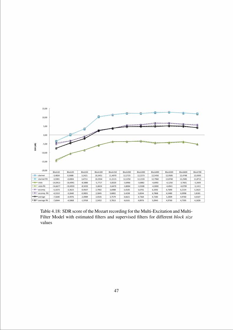
“thesis” — 2013/9/1 — 14:45 — page 47 — #59

Block10 Block20 Block50 Block100 Block150 Block200 Block300 Block400 Block500 Block600 Block700 clarinet -‐3,4834 0,3688 3,2421 10,3451 11,4070 12,2725 12,2273 12,5450 12,9585 12,4748 12,0393

clarinet filt -‐3,5901 -‐0,0004 3,4713 10,2934 11,3115 12,2250 12,2193 12,7960 12,8740 12,2585 11,8713

viola -‐14,0413 -‐10,4991 -‐8,5880 -‐5,7717 -‐3,8320 -‐3,6966 -‐3,6882 -‐4,6992 -‐4,1250 -‐3,7601 -‐5,2693

viola filt -‐14,6677 -‐10,4959 -‐8,5020 -‐5,8424 -‐3,6479 -‐3,8004 -‐3,3508 -‐4,3000 -‐4,4941 -‐4,0799 -‐5,1411

accomp. -‐5,1673 -‐3,3623 -‐0,9507 2,7902 3,6988 5,4105 5,6701 6,3392 6,7690 6,2134 5,2623

accomp. filt -‐4,5553 -‐3,2640 -‐0,9001 2,5845 3,6802 5,4238 5,8244 6,7868 6,5480 6,0998 5,8181

average -‐7,5640 -‐4,4976 -‐2,0989 2,4545 3,7579 4,6621 4,7364 4,7283 5,2009 4,9760 4,0107

average filt -‐7,6044 -‐4,5868 -‐1,9769 2,3452 3,7813 4,6161 4,8976 5,0943 4,9760 4,7595 4,1828

-‐20,00

-‐15,00

-‐10,00

-‐5,00

0,00

5,00

10,00

15,00

SDR (dB)

Table 4.18: SDR score of the Mozart recording for the Multi-Excitation and Multi-Filter Model with estimated filters and supervised filters for different block sizevalues

47

“thesis” — 2013/9/1 — 14:45 — page 48 — #60

- Influence of the Supervised Filter Model Extension for Blind Pitch Estima-tion:

The third and last test of this section tries to measure the influence of the super-vised filter models over a blind pitch estimation process. Until now, the pitchinformation of each instrument to be separated has been provided for all the ex-periments. In this case, the goal is to compare how the timbre models affect thepitch estimation process over the mixture. This is, the pitch is not provided tothe system but it is estimated over the mixture. Two cases of F0 estimation areinspected: when the timbre models are loaded and when they are not (when filtersare estimated).

The parameter configuration for this test is obtained from the results of theparameter optimization test (see Section 4.3.2).

Results

As the goal is not to compare the separation performance but the pitch estimation,the results can not be evaluated with the objective metrics. Instead, the differentestimated F0 matrices are compared.

For the MEF IMM with estimated filters, in order to know which pitch corre-sponds to each instrument the estimations have to be compared to the annotationreference. As the model performs a free separation, the output of the instrumentsis in principle unknown. In our case, since the amount of instruments is reducedan a reference of each instruments pitch is available, we are able to label eachoutput.

Tables 4.3, 4.4, 4.5 and 4.6 depict that the MEF IMM when the supervisedtimbre models are loaded performs a better pitch estimation than the MEF IMMwhen the filters are estimated. The melody lines appear more defined, with lessmissing segments and errors, especially for the clarinet excerpt. This may becaused by the fact that the harmonic series of the clarinet has missing partials,this is, because of its cylindrical resonator, only the odd-numbered harmonics arepresent. This characteristic may be easily modeled when the timbre model issupervised and not estimated from the mixture.

48

“thesis” — 2013/9/1 — 14:45 — page 49 — #61

Figure 4.3: Pitch estimations of a 8 second violin excerpt (Schubert recording).Estimations with Yin (top), MEF IMM (middle) and MEF IMM loading super-vised timbre models (bottom).

Figure 4.4: Pitch estimations over a 8 second cello excerpt (Schubert recording).Estimations with Yin (top), MEF IMM (middle) and MEF IMM loading super-vised timbre models (bottom).

49

“thesis” — 2013/9/1 — 14:45 — page 50 — #62

Figure 4.5: Pitch estimations over a 8 second viola excerpt (Mozart recording).Estimations with Yin (top), MEF IMM (middle) and MEF IMM loading super-vised timbre models (bottom).

Figure 4.6: Pitch estimations over a 8 second clarinet excerpt (Mozart recording).Estimations with Yin (top), MEF IMM (middle) and MEF IMM loading super-vised timbre models (bottom).

50

“thesis” — 2013/9/1 — 14:45 — page 51 — #63

Chapter 5

CONCLUSIONS AND FUTUREWORK

The present work in this master thesis has focused on the study, combination andimprovement of different source separation models. The main motivation was tofind whether the use of instrument dependent source and filter model representa-tions and the use of trained timbre models could help to improve the separationprocess. An existing source separation model, the IMM, has been used as a start-ing point. Overcoming the limitations of the model, modifications over the source/ filter representation have been introduced. More precisely, for the filter sub-model, the use of trained timbre models has been studied. The different resultsshow that the proposed extension of the source / filter model can improve the re-sults of the separation and that the followed methodology is promising, with manypossibilities for further research and potential applications.

5.1 ContributionsThe following list contains the main contributions of this work:

• The literature review done in the related areas of research have determinedthat there is a large amount of research done in source separation and hisdifferent methods and strategies, but the application and performance ofthis methods is still novel for instruments of similar timbre.

• It has been demonstrated how the proposed extensions of modeling the datausing multiple sources and filters allow to improve the quality of the results.

• The relative improvement of the performance of the proposed model overthe IMM model is between 6 dB and 12 dB of SDR, depending on thecontent of the audio mixture.

51

“thesis” — 2013/9/1 — 14:45 — page 52 — #64

• The use of individual instrument data to obtain Trained Timbre Models,which allows to improve the quality of the pitch estimation.

5.2 ConclusionsConsidering the motivations and goals presented in the introduction and havinginto account the above presented contributions, some conclusions can be obtained.

In this thesis, an efficient method for score-informed source separation has benpresented. It specifically uses a source / filter decomposition in a NMF framework,where each one of the instruments present in the mixture is modeled. This pro-posed Multi-Excitation and Filter IMM method produces acceptable audio results,and appears to give better performance results than the compared method from theliterature. This improvement is obtained thanks to the ability of the method to es-timate the representation of each of the instruments with its own source and filtersub-models. Its strength is that the informed pitch estimation provides a good ref-erence of the harmonic parts of each instrument over the decomposition process.However, a weak point is that all the residual or inharmonic parts are not modeledand are fitted into the estimated accompaniment track.

Depending on the application of the method, this fact can be an inconvenientto a certain extent. If the goal is to obtain a total separation of the sources with lis-tening purposes, i.e. ’de-soloing’, the separation of only the harmonic part of theinstrument may not be acceptable. In contrast, if the objective is to apply the sepa-rated sources for remixing, i.e., equalizing or changing the dynamics, the methodcould be totally valid, since the in-harmonic parts have not such a big effect in thiscase.

Regarding the use of trained timbre models, the results show no significantimprovement over the estimation of the timbre directly from the audio mixture.The proposed Multi-Excitation and Filter IMM seems to be able to efficiently es-timate the filter activations directly from the mixture. Further research has to beperformed in the design of the filter to properly adapt it to the specific timbre char-acteristics of the different instruments. However, leaving apart the pitch-informedseparation, the use of this trained timbre models appears to provide a better pitchestimation than the one obtained without any timbre information of the instru-ments. This may show us a new path to follow in further research.

52

“thesis” — 2013/9/1 — 14:45 — page 53 — #65

5.3 Future workSome positive results have been obtained with the proposed models, but the differ-ent steps over the process have shown that there is still a lot of room for improve-ment. In order to obtain more accurate results and a higher quality separationthere are many different aspects that can be worked on.

5.3.1 Source / Filter Model ImprovementsAs it has been mentioned in the conclusions, the proposed model only takes intoaccount the harmonic part of the sources for the decomposition. The extensionof the source / filter model with a transient detection, i.e. a non-harmonic signalmodeling, will potentially improve the results of the separation. Adding somenon-harmonic bases to the NMF decomposition framework is definitely an aspectto work on.

In addition, the proposed model employs a very simple approach for the mod-eling of the source, where the bases are defined by a flat harmonic-comb exci-tation. Adapting this source excitation bases to each of the different instrumentexcitations is also a facet to improve. For example, the introduction of differentexcitation slopes over the harmonic-comb could be a simple and effective startpoint.

5.3.2 Trained Filter Models ImprovementsThe timbre models on the proposed extension are trained by learning the activa-tions over some smooth elementary filters (Hann functions) that represent timbralcharacteristics of the different instruments. The use of this representation appearsto be valid for the estimation of this characteristics over the mixture, but may beimproved with the use of other elementary filters. Instead of using Hann filters,other function combinations should be tested to verify the best possible timbremodeling. For example, the use of wide Gaussian functions to capture the energyzones and narrower ones, with a sparsity constrain, to define the resonances of thespectrum of the instruments can be an option to inspect.

In accordance with the modeling of the non-harmonic parts, inspecting theresidual obtained from the actual timbre model training could provide a good ref-erence to know which requirements are needed to model this transitions.

As the use of this trained timbre models over the pitch estimation depicts apromising result, the use of this information for multi-pitch estimation over themixture audio should be a field to keep on working. The use of pitch-informedsource separation is a good alternative to avoid the problems that state of the art

53

“thesis” — 2013/9/1 — 14:45 — page 54 — #66

multi-pitch estimation algorithms entail, but prior information of the sources isnot always available. In this sense, with only having the information of the instru-ments present in the mixture, another supervised source separation methodology,where timbre information of the instruments is provided, could be followed.

54

“thesis” — 2013/9/1 — 14:45 — page 55 — #67

Appendix A

APPENDIX A

55

“thesis”—

2013/9/1—

14:45—

page56

—#68

BSS Eval results for the Schubert excerpt of the parameter optimization test explained in 4.3.2.

!"# !$# !%# !"# !$# !%# !"# !$# !%# !"# !$# !%# !"# !$# !%# !"# !$# !%#&'()() **'+,- .'/,, &'&&)) **'/-( /'0).. &'.00/ **'()& /'-*&) &'/*+) **',-& /'-*/* &'.-*. **',&- /'0/// &'&-+- **'*+) /'---&&'/.)* *&'+() .')*0- &'/,++ *.'0-) .')-+& &',.** *.'*./ .'),+/ .'0-)* *('/.) .'/,+ .'0((( *&'0&) .'/.*- .'-)&( *&'0/ .'+//*&'+,+- /'/((& **'((. &',//( /'()-- **',*( &'/+&. /'-(&, *-'0*( .'(./ ,'-*() **',/. .'),.- ,'*/*( **'/-& .'(/0, ,'-+)* **'/--&'/-,+ **',,+, ,'*,*( &'/(0- **'/-.( ,')+)( &'/&-& **'.*&+ ,'&)+/ .'0.+, **'.00, ,'.-/( .'0*/( **'.+-* ,'&-*) .'0/,& **'&*,/ ,'.(0&&'0&) **'(.- .'(/+, &'/-*) **'.+) /'-/*/ &'/+0, *-'0&( /'--(. &'.*-- **'&0* /'-0)( &'.&-) **'/(- /'*.0- &'&(,. *0',*, /'(-&+(',0-) *('/. &'(0/( &'(--, *('.&( .'*-* &'),.+ *)'.// .'-..* &'.-&( *)',+, .'(+,, &'/)* *)'.0/ .'.,+( .'*),- *('(&( .'+,)/&'//-/ ,'00- *0')/( .'&/, +'*(,* *0'&// .'+&* +'..., *0'/-) /'0(-, +',&+& *0'.,) /'*/&* *0'0/. *0'/0& /')+, *0'/+. *0')++&'-0+) **'(0,0 /'(-0( &'+0/( **',)*/ /'+,++ .'0(-+ **'/++) ,'0/*- .'0+)& **'/&-, ,'*-,( .'*,.* **',0,) ,'*,(+ .').*. *-'0--/ ,'-.+&&'&-/- **'0)- /'-+-/ &',0)( *-'*&* /'-0&/ &'/0++ **'+0- /'*/&( &'/,.& **'.*- /')+-/ &'/0)* **')+) /')/-, &'&.*/ **'-, /'--,.&'&(&- *.'&*) .'00)- .'0)+, *('.-+ .',))/ .'**,( *('(+* .'+&-, .'-&&/ *(',-. /'0(.) .')0&/ *('... /'*).( .'-.0, *('*/- /'*+0-.'(&0( +'**-( *0')(- /')/(* *0'&,/ *0'&&& /')-.( *0'&.) *0'(,/ /'&*& **'0-/ *0'(0. /'&. **'0.- *0'(&. /',0.+ **',(+ *0'-&+&',(0+ *-'-*+* /',/+) .'(0&, *-'(&&/ ,'*+,* .'),(+ *-')*,/ ,'-0&* .'&*+* *-'(,,) ,'-,*/ .'&--+ *-')/)/ ,')-*/ .'&()* *-'())/ ,'--&+&'.-.+ *-'),. .',++( &'.(*+ *-'0& /'0)-- &'(*-, *0'/&- /'-.. &'.+-+ **'//( /'-0*. &'&./) **')./ /'*+,, &'/0(* **'&-* /')*+)&'&(&) *('(-- .')0*+ &'+-&. *('(/- .'/)*, &'+*+& *&'-*/ .'&+*( .'-+,* *('&*, /'*&,* .'-,.) *(')(& /'*,*/ .'-+(, *('-.) /'-0++.'+.0& +',,)- *0'(,& /'-*-/ *0'-& *0'&,/ .',*(/ +'/(.. *0')(- /'/&)) **'(.) *0'(.* /'.)-( **'()& *0'-/( /',-/( **'.+, *0'(0(.'0((- *-'-)0( /',+&( .'-.0* *-'-&/) ,'**/0 .'0(+0 **'+0&- ,'0..& .'&,*( *-'&,&0 ,'-/). .'(+&) *-'),-) ,'-*,- .'.0,, *-'(+(0 ,')***

*01$234526789

:*0

:)0

:/0

:+0

;* ;- ;) ;*0 ;-0 ;)0

Table A.1: BSS Eval results for the Schubert excerpt over 10 iterations and different values for P smooth filters and K bases

56

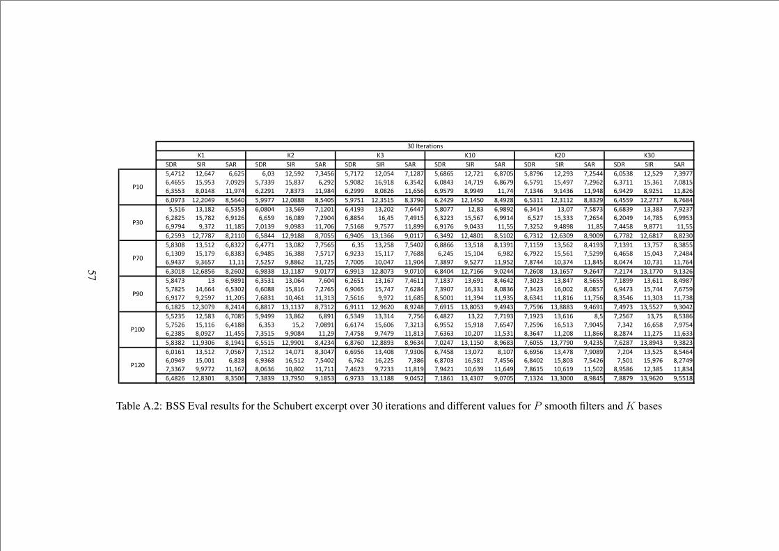
“thesis”—

2013/9/1—

14:45—

page57

—#69

!"# !$# !%# !"# !$# !%# !"# !$# !%# !"# !$# !%# !"# !$# !%# !"# !$# !%#&'()*+ *+',() ,',+& ,'-. *+'&/+ )'.(&, &')*)+ *+'-&( )'*+0) &',0,& *+')+* ,'0)-& &'0)/, *+'+/. )'+&(( ,'-&.0 *+'&+/ )'./)),'(,&& *&'/&. )'-/+/ &')../ *&'0.) ,'+/+ &'/-0+ *,'/*0 ,'.&(+ ,'-0(. *(')*/ ,'0,)/ ,'&)/* *&'(/) )'+/,+ ,'.)** *&'.,* )'-0*&,'.&&. 0'-*(0 **'/)( ,'++/* )'0.). **'/0( ,'+/// 0'-0+, **',&, ,'/&)/ 0'//(/ **')( )'*.(, /'*(., **'/(0 ,'/(+/ 0'/+&* **'0+,,'-/). *+'+-(/ 0'&,(- &'//)) *+'-000 0'&(-& &'/)&* *+'.&*& 0'.)/, ,'+(+/ *+'*(&- 0'(/+0 ,'&.** *+'.**+ 0'0.+/ ,'(&&/ *+'+)*) 0'),0(&'&*, *.'*0+ ,'&.&. ,'-0-( *.'&,/ )'*+-* ,'(*/. *.'+-+ )',(() &'0-)) *+'0. ,'/0/+ ,'.(*( *.'-) )'&0). ,',0./ *.'.0. )'/+.),'+0+& *&')0+ ,'/*+, ,',&/ *,'-0/ )'+/-( ,'00&( *,'(& )'(/*& ,'.++. *&'&,) ,'//*( ,'&+) *&'... )'+,&( ,'+-(/ *(')0& ,'//&.,'/)/( /'.)+ **'*0& )'-*./ /'-/0. **')-, )'&*,0 /')&)) **'0// ,'/*), /'-(.. **'&& )'.+&+ /'(0/0 **'0& )'((&0 /'0))* **'&&,'+&/. *+'))0) 0'+**- ,'&0(( *+'/*00 0')-&& ,'/(-& *.'*.,, /'-**) ,'.(/+ *+'(0-* 0'&*-+ ,').*+ *+',.-/ 0'/--/ ,'))0+ *+',0*) 0'0+.-&'0.-0 *.'&*+ ,'0.++ ,'())* *.'-0+ )')&,& ,'.& *.'+&0 )'&(-+ ,'00,, *.'&*0 0'*./* )'**&/ *.'&,+ 0'(*/. )'*./* *.')&) 0'.0&&,'*.-/ *&'*)/ ,'0.0. ,'/(0& *,'.00 )'&)*) ,'/+.. *&'**) )'),00 ,'+(& *&'*-( ,'/0+ ,')/++ *&'&,* )'&+// ,'(,&0 *&'-(. )'+(0(,'/(.) /'.,&) **'** )'&+&) /'00,+ **')+& )')--& *-'-() **'/-( )'.0/) /'&+)) **'/&+ )'0)(( *-'.)( **'0(& 0'-()( *-').* **'),(,'.-*0 *+',0&, 0'+,-+ ,'/0.0 *.'**0) /'-*)) ,'//*. *+'0-). /'-)*- ,'0(-( *+')*,, /'-+(( )'+,-0 *.'*,&) /'+,() )'+*)( *.'*))- /'*.+,&'0(). *. ,'/0/* ,'.&.* *.'-,( )',-( ,'+,&* *.'*,) )'(,** )'*0.) *.',/* 0'(,(+ )'.-+. *.'0() 0'&,&& )'*0// *.',** 0'(/0)&')0+& *(',,( ,'&.-+ ,',-00 *&'0*, )'+),& ,'/-,& *&')() )',+0( )'./-) *,'..* 0'-0., )'.(+. *,'--+ 0'-0&) ,'/(). *&')(( )',)&/,'/*)) /'+&/) **'+-& )',0.* *-'(,* **'.*. )'&,*, /'/)+ **',0& 0'&--* **'./( **'/.& 0',.(* **'0*, **')&, 0'.&(, **'.-. **').0,'*0+& *+'.-)/ 0'+(*( ,'00*) *.'**.) 0').*+ ,'/*** *+'/,+- 0'/+(0 )',/*& *.'0-&. /'(/(. )')&/, *.'000. /'(,/* )'(/). *.'&&+) /'.-(+&'&+.& *+'&0. ,')-0& &'/(// *.'0,+ ,'0/* ,'&.(/ *.'.*( )')&, ,'(0+) *.'++ )')*/. )'*/+. *.',*, 0'& )'+&,) *.')& 0'&.0,&')&+, *&'**, ,'(*00 ,'.&. *&'+ )'-0/* ,',*)( *&',-, )'.+*. ,'/&&+ *&'/*0 )',&() )'+&/, *,'&*. )'/-(& )'.(+ *,',&0 )'/)&(,'+.0& 0'-/+) **'(&& )'.&*& /'/-0( **'+/ )'()&0 /')()/ **'0*. )',.,. *-'+-) **'&.* 0'.,() **'+-0 **'0,, 0'+0)( **'+)& **',..&'0.0+ **'/.-, 0'*/(* ,'&&*& *+'//-* 0'(+.( ,'0),- *+'00/. 0'/,.( )'-+() *.'**&- 0'/,0. )',-&& *.'))/- /'(+.& )',+0) *.'0/(. /'.0+.,'-*,* *.'&*+ )'-&,) )'*&*+ *('-)* 0'.-() ,',/&, *.'(-0 )'/.-, ,')(&0 *.'-)+ 0'*-) ,',/&, *.'()0 )'/-0/ )'+-( *.'&+& 0'&(,(,'-/(/ *&'--* ,'0+0 ,'/.,0 *,'&*+ )'&(-+ ,'),+ *,'++& )'.0, ,'0)-. *,'&0* )'(&&, ,'0(-+ *&'0-. )'&(+, )'&-* *&'/), 0'+)(/)'..,) /'/))+ **'*,) 0'-,., *-'0-+ **')** )'(,+. /')+.. **'0*/ )'/(+* *-',./ **',(/ )'0,*& *-',*/ **'&-+ 0'/&0, *+'.0& **'0.(,'(0+, *+'0.-* 0'.&-, )'.0./ *.')/&- /'*0&. ,'/).. *.'**00 /'-(&+ )'*0,* *.'(.-) /'-)-& )'*.+( *.'.--- 0'/0(& )'00)/ *.'/,+- /'&&*0

1.-.-2$34563789:

1* 1+ 1. 1*- 1+-

;*--

;*+-

;*-

;.-

;)-

;/-


57

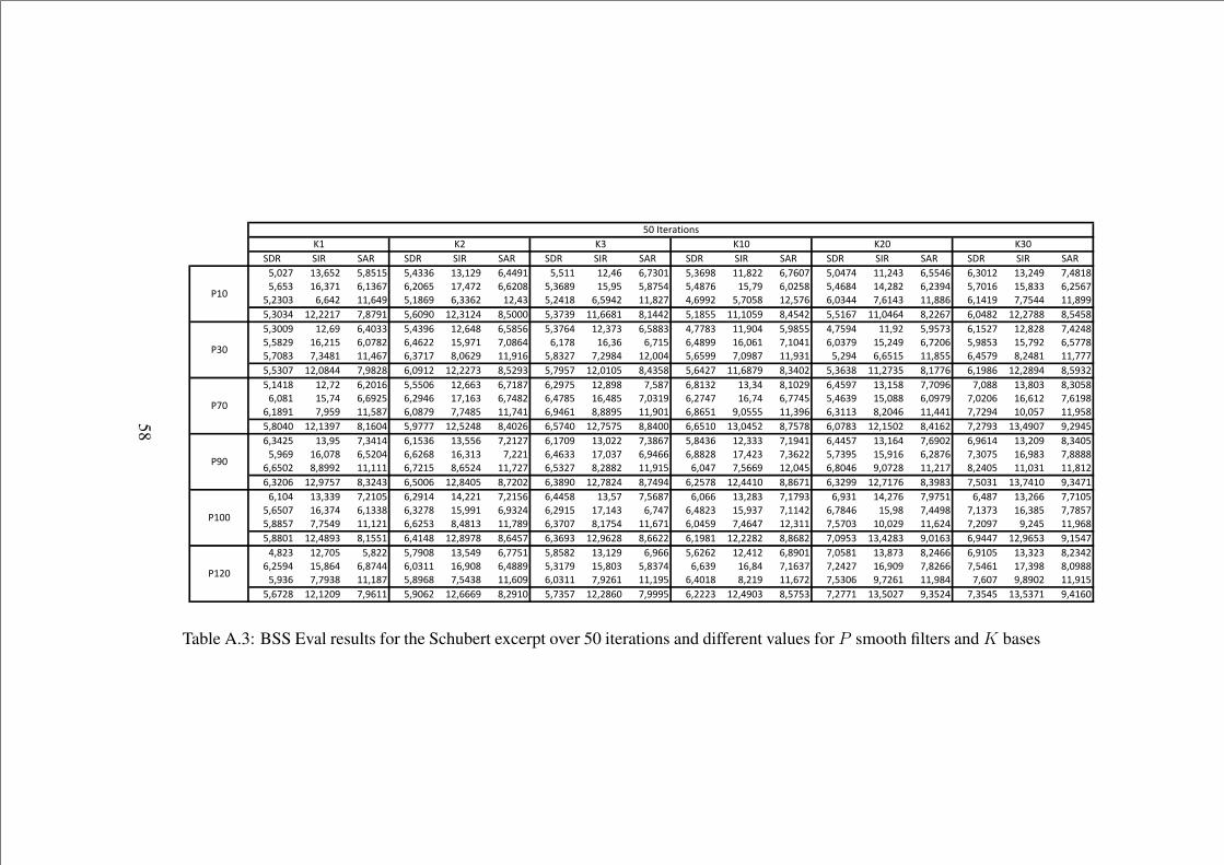
“thesis”—

2013/9/1—

14:45—

page58

—#70

!"# !$# !%# !"# !$# !%# !"# !$# !%# !"# !$# !%# !"# !$# !%# !"# !$# !%#&'()* +,'-&) &'.&+& &'/,,- +,'+)0 -'//0+ &'&++ +)'/- -'*,(+ &',-0. ++'.)) -'*-(* &'(/*/ ++')/, -'&&/- -',(+) +,')/0 *'/.+.&'-&, +-',*+ -'+,-* -')(-& +*'/*) -'-)(. &',-.0 +&'0& &'.*&/ &'/.*- +&'*0 -'()&. &'/-./ +/').) -'),0/ &'*(+- +&'.,, -')&-*&'),(, -'-/) ++'-/0 &'+.-0 -',,-) +)'/, &')/+. -'&0/) ++'.)* /'-00) &'*(&. +)'&*- -'(,// *'-+/, ++'..- -'+/+0 *'*&// ++'.00&',(,/ +)'))+* *'.*0+ &'-(0( +)',+)/ .'&((( &',*,0 ++'--.+ .'+//) &'+.&& ++'+(&0 .'/&/) &'&+-* ++'(/-/ .'))-* -'(/.) +)')*.. .'&/&.&',((0 +)'-0 -'/(,, &'/,0- +)'-/. -'&.&- &',*-/ +)',*, -'&.., /'**., ++'0(/ &'0.&& /'*&0/ ++'0) &'0&*, -'+&)* +)'.). *'/)/.&'&.)0 +-')+& -'(*.) -'/-)) +&'0*+ *'(.-/ -'+*. +-',- -'*+& -'/.00 +-'(-+ *'+(/+ -'(,*0 +&')/0 -'*)(- &'0.&, +&'*0) -'&**.&'*(., *',/.+ ++'/-* -',*+* .'(-)0 ++'0+- &'.,)* *')0./ +)'((/ &'-&00 *'(0.* ++'0,+ &')0/ -'-&+& ++'.&& -'/&*0 .')/.+ ++'***&'&,(* +)'(.// *'0.). -'(0+) +)'))*, .'&)0, &'*0&* +)'(+(& .'/,&. &'-/)* ++'-.*0 .',/() &',-,. ++')*,& .'+**- -'+0.- +)').0/ .'&0,)&'+/+. +)'*) -')(+- &'&&(- +)'--, -'*+.* -')0*& +)'.0. *'&.* -'.+,) +,',/ .'+()0 -'/&0* +,'+&. *'*(0- *'(.. +,'.(, .',(&.-'(.+ +&'*/ -'-0)& -')0/- +*'+-, -'*/.) -'/*.& +-'/.& *'(,+0 -')*/* +-'*/ -'**/& &'/-,0 +&'(.. -'(0*0 *'()(- +-'-+) *'-+0.-'+.0+ *'0&0 ++'&.* -'(.*0 *'*/.& ++'*/+ -'0/-+ .'..0& ++'0(+ -'.-&+ 0'(&&& ++',0- -',++, .')(/- ++'//+ *'*)0/ +('(&* ++'0&.&'.(/( +)'+,0* .'+-(/ &'0*** +)'&)/. .'/()- -'&*/( +)'*&*& .'./(( -'-&+( +,'(/&) .'*&*. -'(*., +)'+&() .'/+-) *')*0, +,'/0(* 0')0/&-',/)& +,'0& *',/+/ -'+&,- +,'&&- *')+)* -'+*(0 +,'()) *',.-* &'./,- +)',,, *'+0/+ -'//&* +,'+-/ *'-0() -'0-+/ +,')(0 .',/(&&'0-0 +-'(*. -'&)(/ -'-)-. +-',+, *'))+ -'/-,, +*'(,* -'0/-- -'..). +*'/), *',-)) &'*,0& +&'0+- -').*- *',(*& +-'0., *'....-'-&() .'.00) ++'+++ -'*)+& .'-&)/ ++'*)* -'&,)* .')..) ++'0+& -'(/* *'&--0 +)'(/& -'.(/- 0'(*). ++')+* .')/(& ++'(,+ ++'.+)-',)(- +)'0*&* .',)/, -'&((- +)'./(& .'*)() -',.0( +)'*.)/ .'*/0/ -')&*. +)'//+( .'.-*+ -',)00 +)'*+*- .',0., *'&(,+ +,'*/+( 0',/*+-'+(/ +,',,0 *')+(& -')0+/ +/'))+ *')+&- -'//&. +,'&* *'&-.* -'(-- +,')., *'+*0, -'0,+ +/')*- *'0*&+ -'/.* +,')-- *'*+(&&'-&(* +-',*/ -'+,,. -',)*. +&'00+ -'0,)/ -')0+& +*'+/, -'*/* -'/.), +&'0,* *'++/) -'*./- +&'0. *'//0. *'+,*, +-',.& *'*.&*&'..&* *'*&/0 ++'+)+ -'-)&, .'/.+, ++'*.0 -',*(* .'+*&/ ++'-*+ -'(/&0 *'/-/* +)',++ *'&*(, +('()0 ++'-)/ *')(0* 0')/& ++'0-.&'..(+ +)'/.0, .'+&&+ -'/+/. +)'.0*. .'-/&* -',-0, +)'0-). .'--)) -'+0.+ +)')).) .'.-.) *'(0&, +,'/)., 0'(+-, -'0//* +)'0-&, 0'+&/*/'.), +)'*(& &'.)) &'*0(. +,'&/0 -'**&+ &'.&.) +,'+)0 -'0-- &'-)-) +)'/+) -'.0(+ *'(&.+ +,'.*, .')/-- -'0+(& +,',), .'),/)-')&0/ +&'.-/ -'.*// -'(,++ +-'0(. -'/..0 &',+*0 +&'.(, &'.,*/ -'-,0 +-'./ *'+-,* *')/)* +-'0(0 *'.)-- *'&/-+ +*',0. .'(0..&'0,- *'*0,. ++'+.* &'.0-. *'&/,. ++'-(0 -'(,++ *'0)-+ ++'+0& -'/(+. .')+0 ++'-*) *'&,(- 0'*)-+ ++'0./ *'-(* 0'.0() ++'0+&&'-*). +)'+)(0 *'0-++ &'0(-) +)'---0 .')0+( &'*,&* +)').-( *'000& -'))), +)'/0(, .'&*&, *')**+ +,'&()* 0',&)/ *',&/& +,'&,*+ 0'/+-(

1+ 1) 1, 1+( 1)( 1,(&(2$34563789:

;+(

;,(

;*(

;0(

;+((

;+)(


58

“thesis”—

2013/9/1—

14:45—

page59

—#71

!"# !$# !%# !"# !$# !%# !"# !$# !%# !"# !$# !%# !"# !$# !%# !"# !$# !%#&'(()& (*'+), -'(-*& .'+/&- (('// -'00(/ &'0&,. (*'*(/ -'*.0. &'(&,, ((',0( -'.-& .',,+, (('/*- -'*/.& .'..( (*'(- &'&0(,.'///- (+'.(& &'*(-& &'+*(/ (/'&0& -'0(++ &'(/0) (-'.&- &'-()/ &'/(/, (+'*++ -'**(& &'0( (-'-() &'.(., .'+&*& (&'&,, &'*.)&)',.+ .'+(*) ()'(*/ .'-+*+ &'/)(& ((',/& .'*+, &'(..( (*'/+ .')&.- &'**,& (*'//* .'+,-- -'00.& ((',(+ .')-,& &'&&&* (('-&).'-.,+ (('-**( /'(-,0 &'0-00 (*'0+** /'00(& .'/),- (('*+*+ /'*.(. &'(((( (('.-,* /'&**/ .',)./ (('./(* +'/+*( .'&*(0 (('(0.+ +'.--(.'-+/* (*'/*/ &'-*0/ &'0*-. (*'-/ -'0+*. &'(+&* (*'-,* -'*.,. .',)/+ (*'**& -'0/,) .',(/ (*'*(( -'0-+, &'))0/ (*'+,) -'.((,&',0&. (-'-+, -')++) -'*-(/ (-',/+ -'+)(, &'-.&- (&'/*+ -'(,&& &'-/0* (-'&,+ -'(.0, -'-/(/ (.',,. +'&(0* -')00) (&'.& -',/&&.',*-- -'(-0* ((',)- &')(&. -'-&)- ((',) .'/&+( &',0) (*'&.& .'+0+( &'+,,- (*'*& &'/)( +'**(( (*'*0, &'),. -'-*() (*'))+&'(+0( (('//,( +',+/0 &'&).& (*'(0-, /'*../ &'**-0 (('.+.0 /'))00 &'(0/+ (('&.0& /'(-0( &'/(0) (('.+&. /'&,&+ &'-+&0 (('-*(. /'&+/(&'(/0* (*'&(( -')0&* &'&)0+ (*'-+ -'-,(/ .'-/*. (*'**. &'++-& -'(/+. ()'&,) +'*..) -'&0&/ ()'+&, +'&,0& -'.(-) ()'(&( +'-&-,&')-. (-'0-( &'/&-, -'(+-) (+',0/ -'&.+/ .'.-/ (-'*)/ .'/-,( &'-,-/ (&'-*- -'*+,- -'/0- (+').& +'*/-, &'++.) (-'.(- -'*-.(&'0.+( -'*/0. (*'0). &')(+( -'&*() (*')& .')..- &'&+)& (('., &',0& +'&,+, (('&(* -'-&-- /'&/.( (('-+- -'*0(, +',,,/ (('&),&'(,+( (('-(+& /'0-&. &'-+.+ (*')--. /'&*,, .'.,/) ((').&* +')+/& &',*,+ (*'*+*) /').&) -'-&-( ()'**,. /'/&(( -'()0/ (*'&**) /'./-+&'&)&/ ()',*. -')//* &'&+(& (*'&)) -'+/)& &'/,-& ()'0,/ +'0**( -'*-.. ()'(-) +'.-(. +'())+ ()'/,/ /')).- &',)0* ()')./ -',,&(-'.&+* (+')./ -',0&. &'--*+ (+'*&. -'0&&- &').++ (&'/)/ &'/-&, &'/&*( (-',- -'*/, &'0.(& (&'&)- &'&-+* &')-.) (&'-/* &',0)/&'(00* -'*.&) (*')+. .',+*/ -'(*.) (*'*& &'.,.+ -',0-( (('/-, -'00,/ +'+-)) (('.-/ -'),,, /'.*&& (('*-, &'/++) +',(-( (0'+,*&'-,++ (*'&0&/ /'&&&, &'.0*) ((',+0. /')-)0 &'&+,- ((',.+. /'*&*) -'0.*( (*'-*// /'.0-( -'(,(+ (*'-(,/ /'),0) &'+*), (*')(&. +'/,+0&'*)+/ (*'--, -'))*( &'-+** (*'+,/ -'/)0) .'/+,) (('/,+ -'(()& .',)/+ (*')+* -'0./* &',+& ()'0.) +'()&( -'.),+ ()'.** +'-0),&'/(./ (-'0-* -')&* &'/(&/ (+'*&, -'*(,, &',*)/ (/'0)+ -'*-+ &'/-/. (&'/,- -'.))* &'+,-/ (+'*,/ -'(,&+ -'+,&. (-'0-) +'../+&'-0,- +'0,,. (('+&) &'.).* -'/+.. (('+), .'-*-) &'-./+ (*'.&& &'),,* -'/+&+ (('-() -'*- /'*/(- (('(&. +'*)*/ ,').,. (('/.+&'&&.( ((',.)& /'(.&+ &'-.0+ (*')(0& /'*-)( &'(.)( (('/-0, /'*+/& &'.0*( (('+(.- /'0)(& -'0(0- (*'/+.* /'(-(- -'/**- (*',../ /',--&&'0&&( (*')(( -'*0/ -'00*& (*',+( +'(,0+ &'/)., ()'(** -',),. -'&++, (.'(0- +'&/+/ -'**,/ (*'/,( +'&0*/ -'&*/. ()'.*+ +'+().&'((*/ (-'-+( &'&(,/ &'--* (+',.* &',,- &'&*,+ (+'-*& &'//0/ -'*(-/ (-'&0/ -'+),) -'-/* (-',/ +'(,)/ -'/&./ (-'++. +'.((/.'+&,- &',/)+ (('/)) .'+-0& &'+.0+ (*'+)) .'//*( -'0.*, (*'(.& -')*&, /'0)0( (('/./ -'*(&- +'/0*/ (*'0*) +'(*+/ ,'./). ((')+).',+&/ (('-&&* +'/&)- &'.+&0 (*'*(+, /'-),, &'.(&- (*'*-)) /')*(+ -')+)& (*'//(. /'+*&0 -')+&/ (*'&&+, /',0-& -'/)+0 ()'**/( /'/)*+

1( 1* 1) 1(0 1*0 1)0+02$34563789:

;(0

;)0

;+0

;,0

;(00

;(*0


59

“thesis”—

2013/9/1—

14:45—

page60

—#72

!"# !$# !%# !"# !$# !%# !"# !$# !%# !"# !$# !%# !"# !$# !%# !"# !$# !%#&'()(* (*')+ ,'-.., &'**)/ (.'). ,'&..) )',,(& (.'0)& &'&/+( )'/+.* (('/(0 ,'..*. &'.,* (*'/*& ,'-,00 )'&+), (('0&. &'+)/))'++(+ (+'*-, &'(-(( &'&0,, (,'&*& ,'-)&/ )'&//+ (&')). &'-/&* )',)&) (&'-+& &'(/-+ &'(0(+ ()',** &'0&(0 &'()(0 (&'(+& &'+.&+*'/./ )'++,+ (.',0/ )'). &'*.&& (.'+/( *'0)0+ )'+*(. (.'),. *'/&0, )'0--/ (.'+*0 )'.((, &'(-), (.',00 )'&&0 &'+)-, (('0(.)',()- (('0&-/ +'/*+, &'((*0 ((').,0 0')&*( )'*+-- (('--,( +'+(0( )'&.&) (-'&/0- 0'-&-, )'00&) (('..). 0'.-./ )'+&0( (-'/..& +'+,.))'/+/+ (.',&/ ,'-.(, )'/)*( (.'&(& ,'-()0 )',+-0 (.'*), &'+*-* )'(,// ((')/) &'*&,, )')-+/ (('/+, &'&(-/ )')*-( (('0+. &'&,,))'/0&( (,'/+. &'*&&) )'0,0/ (,',0* &'.&,/ )'/(., (+'0.0 &'.(() &'-,,. (,'&,0 &')+/, ,'-*&) (&')/. ,',+0+ &'-0/0 (&'+.* &'&/+.)'(*+, &'-0-( (.')( )'&&0& &'+&.+ (('++* )'.)0( &'**+0 (('/-( )'(,)+ &'**+ (('&) &'(,)* ,'&& ((',,0 )',-,( ,'-,)/ (('-(*)'+--0 (('&+-) +'/./- )'+/-. ((',&-. +',0(, )',(-& (('0*+* +',(). )'),,/ (('(**- +')&0+ &'.-.& (('**/* +'/&.& )'+-0+ (('..-- +'*/..)'0,&/ (.',). &'00/ &'&(0& (.'&,( ,'+-0/ )'*() ((',&, &')0,. &',( (*')(+ ,'&/-( +'*(/ ()'0*, 0'*-, &')*00 (*'*/* ,'*/(*&'+/-0 (+'(-* ,'.-0( &'-&-( (,'0&. &')*&& &'*.&) (,'/&/ &'+.-0 ,',+++ (0'-,( +'-+./ ,'&.., (0'(&. ,'0/++ &',/) (&'*(0 ,'*.(.)'+/,, ,'-&), (('+&) )'0)*) ,'-/&) (('0( )'-0(, &'-.(& (.'*+/ &',+,) +'.,,/ (('&&+ ,')+/* 0'.&) (('0.0 &'+0/, +'&-/* (('*&)&'(&(( (('/**. +'/&-) &'(*+* (('0*,( +'/0)0 )'&+*+ (('.(.. +'0,.- &'/00- (.'/(&- 0')-,+ ,'++*, (*'+)+* /'-(-, &',)-0 (.'-+*) 0'-...&'*-// (.'/(0 ,'*&*, )')/** (('+). &',0(* )'/.)& (.'+&0 &'/*-. ,'*)(( (*'+)( +'*/* +'(,&( ()'.*( 0'.+,) ,'(-), (.'/(0 +'**&(&',)), (,',,/ ,'-/)& &'0/,/ (0'-+/ ,'.*& &'+/,& (+')00 ,'(++/ &')(/, (,'*-. &'0/ &'+./) (&'(+, ,'*0./ ,'&*)* (,')/+ +'-/..&'(&.+ ,'),/ (('0,( )',*** &'+&,, (.'-+/ )',,0& &'+0*+ (.'(*, &')+-) ,'+&,( (.'.(& ,'-&/, +',0.. (('0-& ,',+,) 0',*)) ((',*,&'*,/( (.'-(0+ 0'(-*- &'--+0 (('0&/. +'//0) &'(./0 (.'--// 0'-0() &'+)*+ (.'.,,) 0')//* ,'*(0- (.'*,*( 0'0.() ,')*0) (.',0*( 0',0+0&'*&*0 (.'&&) ,'&-,, &',0++ (*'*** ,'+-)* &'&+(/ (*'-,( ,',*). ,'-+0+ (*'-0/ +'.&-0 ,'/.++ ()'((. 0'-()/ ,'/&*. (*'/,) 0'-00()'/00. (,',00 &'*0)* &',/-. (+'*,+ ,'-+)0 &'++(* (,'/*/ ,'.-*& &'&-&+ (,'+** &'/*+. +'.+&& (,'+(+ +'0/() &'+),. (+'-(& ,'(,0+)'/.. ,'*..& ((')./ &'-&0* ,'.&/* (.'(& )'+0(+ &'0(/, (.'&(+ &'())0 ,'*/&. (.'-&/ ,'++-/ 0'*&,/ (.'&-, &'00/+ +'+(0& (('.-+&'-00- (('0&)0 +'++** &')+0+ (.'*(/0 0'*-/+ &'*+&- (('/*// 0')&(, &'&+,) (.'-+.) 0')(&+ ,'//() (*'-,.- /')+-0 ,'(/,) (.'0//. 0')0+/&'.-+0 (.'+/+ ,'.,(& &'&-0, (.'0// ,',--. &'.,*& (*'*0, ,'(0& ,'/0). ()'-.. 0'((-. ,'/(&+ ()'*(/ +'/)& ,'&**, (*'+0 +',(/(&'.++& (,',*& &'+--+ &'&,,* (+',)* &'/(0) &'/0+0 (+'/0( ,'**// ,',0*/ (0'-&0 +'-0 ,'+-&* (0',&/ +'-&-. &'*-*. (&'-*, &'/.&+&'-/*( ,'),&, ((',)0 &'(.( ,'&-+, ((',* )'++-) &'0(0, (.'),0 ,'(,00 +'&)& (.'&*) ,'(+( +'/,*) (('&.) &'&0 +'((0. ((',-&&'(/.0 (('/,&/ +'0+-( &'*/0, (.'*)// 0'-)/& &'*)-, (.'*/&. 0'**(- ,',(.* (*'.-0* /'.)() ,'&/+* (*',)+( 0'0*/+ &'0-&, (('/+0( 0'*0**

1( 1. 1* 1(- 1.- 1*-/-2$34563789:

;(-

;*-

;+-

;/-

;(--

;(.-


60

“thesis” — 2013/9/1 — 14:45 — page 61 — #73

Appendix B

APPENDIX B

61

“thesis”—

2013/9/1—

14:45—

page62

—#74

SIR and SAR error values of Schubert and Mozart recordings over different iteration values corresponding to the testpresented in 4.3.3.

3iter 5iter 7iter 10iter 15iter 20iter 25iter 30iter 50iter 70iter 90iter violin 19,8926 17,8573 15,6695 14,5564 13,9760 15,1664 14,0037 14,8720 17,8458 16,3979 16,7476

violin filt 19,7308 18,1106 14,9717 12,6488 13,7885 14,0050 13,4238 14,9443 15,7703 16,0260 16,7369

cello 11,1352 10,5233 8,8571 9,3759 9,4785 10,7559 11,5485 12,3566 12,5777 12,2707 13,1644

cello filt 14,7014 13,8496 12,9280 11,6985 10,2647 11,2751 11,3983 12,8391 13,8399 14,0943 12,8329

accomp. 3,9033 7,1252 8,1884 9,7018 10,0439 9,7973 9,8108 9,7730 8,7884 7,5221 7,0757

accomp. filt 0,1958 3,3072 6,0053 8,1506 9,5255 9,7132 10,0710 9,5178 8,5566 8,3675 8,1532

average 11,6437 11,8353 10,9050 11,2113 11,1661 11,9065 11,7877 12,3339 13,0706 12,0636 12,3292

average filt 11,5426 11,7558 11,3017 10,8326 11,1929 11,6644 11,6310 12,4337 12,7223 12,8292 12,5743

0,00

5,00

10,00

15,00

20,00

25,00

SIR (dB)

Table B.1: SIR error of the Schubert recording for the Multi-Excitation and Multi-Filter Model with estimated filters andtrained filters for different iteration values

62

“thesis”—

2013/9/1—

14:45—

page63

—#75

3iter 5iter 7iter 10iter 15iter 20iter 25iter 30iter 50iter 70iter 90iter clarinet 19,1733 17,7808 17,7113 17,7810 17,8058 17,8200 17,6388 17,9463 17,9918 18,2758 18,8958

clarinet filt 20,0425 17,1303 17,3280 17,4515 17,5745 17,7260 17,5200 17,6993 18,2950 17,9300 18,0640

viola 0,5795 1,7123 0,9037 0,5618 0,5442 1,1040 0,5997 0,1295 0,5682 0,2348 0,9245

viola filt 3,8174 6,5438 4,3413 1,1360 0,9429 0,5683 0,4299 0,3893 0,6316 0,4730 0,7251

accomp. 4,1717 10,9620 13,7098 13,8138 13,6938 12,8430 13,4053 11,9483 13,0860 10,7913 9,8143

accomp. filt -‐0,2579 8,1416 10,1032 12,8974 14,2330 13,6268 14,1110 14,3150 13,9710 12,7970 13,9423

average 7,9748 10,1517 10,7749 10,7188 10,6812 10,5890 10,5479 10,0080 10,5486 9,7673 9,8782

average filt 7,8674 10,6052 10,5908 10,4950 10,9168 10,6403 10,6870 10,8012 10,9659 10,4000 10,9104

-‐5,00

0,00

5,00

10,00

15,00

20,00

25,00

SIR (dB)

Table B.2: SIR error of the Mozart recording for the Multi-Excitation and Multi-Filter Model with estimated filters andtrained filters for different iteration values

63

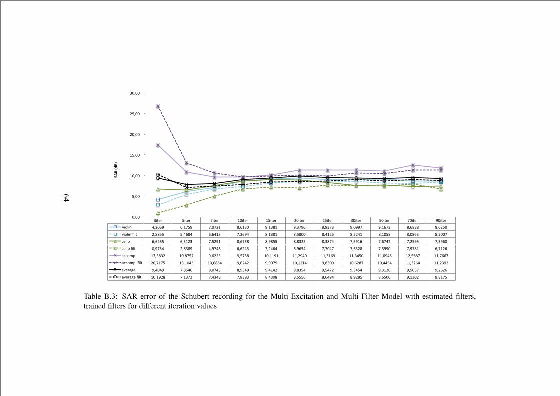
“thesis”—

2013/9/1—

14:45—

page64

—#76

3iter 5iter 7iter 10iter 15iter 20iter 25iter 30iter 50iter 70iter 90iter violin 4,2059 6,1759 7,0721 8,6130 9,1381 9,3796 8,9373 9,0997 9,1673 8,6888 8,6250

violin filt 2,8855 5,4684 6,6413 7,2694 8,1381 8,5800 8,4125 8,5241 8,1058 8,0863 8,5007

cello 6,6255 6,5123 7,5291 8,6758 8,9855 8,8325 8,3874 7,5916 7,6742 7,2595 7,3960

cello filt 0,9754 2,8389 4,9748 6,6243 7,2464 6,9654 7,7047 7,6328 7,3990 7,9781 6,7126

accomp. 17,3832 10,8757 9,6223 9,5758 10,1191 11,2940 11,3169 11,3450 11,0945 12,5687 11,7667

accomp. filt 26,7175 13,1043 10,6884 9,6242 9,9079 10,1214 9,8309 10,6287 10,4454 11,3264 11,2392

average 9,4049 7,8546 8,0745 8,9549 9,4142 9,8354 9,5472 9,3454 9,3120 9,5057 9,2626

average filt 10,1928 7,1372 7,4348 7,8393 8,4308 8,5556 8,6494 8,9285 8,6500 9,1302 8,8175

0,00

5,00

10,00

15,00

20,00

25,00

30,00

SAR (dB)

Table B.3: SAR error of the Schubert recording for the Multi-Excitation and Multi-Filter Model with estimated filters,trained filters for different iteration values

64

“thesis”—

2013/9/1—

14:45—

page65

—#77

3iter 5iter 7iter 10iter 15iter 20iter 25iter 30iter 50iter 70iter 90iter clarinet 11,2444 13,5613 14,0863 14,1318 14,0628 14,1373 14,0998 13,9955 14,1543 13,6550 13,4618

clarinet filt 10,7713 12,5543 13,7250 14,1758 14,3253 14,3818 14,1995 14,2720 14,2860 13,8923 14,1968

viola -‐0,7345 3,1182 3,9351 4,7457 5,0027 5,0645 5,0194 4,9079 4,9732 4,6150 4,6946

viola filt -‐11,3382 -‐11,0941 -‐5,0338 -‐1,3281 -‐0,2847 0,5026 0,7427 1,0461 0,7530 1,9040 1,1534

accomp. 11,0368 8,7273 8,2431 8,4307 8,3800 8,4118 8,4176 8,2711 8,7650 8,7463 8,5493

accomp. filt 2,1821 7,6346 8,9347 8,2232 8,2136 8,4278 8,1727 8,2763 8,5530 8,1535 8,6597

average 7,1823 8,4689 8,7548 9,1027 9,1485 9,2045 9,1789 9,0582 9,2975 9,0054 8,9019

average filt 0,5384 3,0316 5,8753 7,0236 7,4181 7,7707 7,7050 7,8648 7,8640 7,9832 8,0033

-‐15,00

-‐10,00

-‐5,00

0,00

5,00

10,00

15,00

20,00

SAR (dB)

Table B.4: SAR error of the Mozart recording for the Multi-Excitation and Multi-Filter Model with estimated filters andtrained filters for different iteration values

65

“thesis”—

2013/9/1—

14:45—

page66

—#78

SIR and SAR error values of Schubert and Mozart recordings over different block size values corresponding to the testpresented in 4.3.3.

Block10 Block20 Block50 Block100 Block150 Block200 Block300 Block400 Block500 Block600 Block700 violin 8,50418 14,41708 13,39212 18,18635 16,60117 17,13912 16,16410 15,66495 16,51865 15,36448 16,18713

violin filt 10,48158 13,35117 16,58977 16,49122 15,38913 17,02967 17,16715 15,67672 15,17485 15,18492 15,75893

cello 6,61620 9,29285 9,74283 12,45767 10,14300 11,10080 12,08295 11,40525 10,24067 11,18913 12,89950

cello filt 5,19405 9,70233 9,98312 12,78693 9,55943 10,84342 11,51422 11,62672 10,34410 11,19415 13,31348

accomp. 3,91852 0,00470 1,27750 3,32451 3,78593 6,16138 6,83475 7,81785 8,40350 8,50247 8,19582

accomp. filt 3,48006 -‐0,02867 1,45225 3,18548 3,89134 5,68663 7,38138 8,17107 8,52703 8,61720 8,94108

average 6,34630 7,90488 8,13748 11,32284 10,17670 11,46710 11,69393 11,62935 11,72094 11,68536 12,42748

average filt 6,38523 7,67494 9,34171 10,82121 9,61330 11,18657 12,02092 11,82483 11,34866 11,66542 12,67117

-‐5,00

0,00

5,00

10,00

15,00

20,00

SIR (dB)

Table B.5: SIR error of the Schubert recording for the Multi-Excitation and Multi-Filter Model with estimated filters andtrained filters for different block size values

66

“thesis”—

2013/9/1—

14:45—

page67

—#79

Block10 Block20 Block50 Block100 Block150 Block200 Block300 Block400 Block500 Block600 Block700 clarinet 14,80223 16,23135 20,54725 21,70400 20,39675 19,87100 19,66500 18,11050 19,30500 19,55775 18,92825

clarinet filt 15,85118 16,54790 20,62175 21,06525 19,53025 19,80550 19,49200 18,31175 19,45625 19,31250 18,63575

viola -‐4,11718 -‐1,57781 0,57600 3,27125 4,11800 3,82120 2,12915 0,39913 1,34183 1,17725 -‐0,74380

viola filt -‐2,23300 -‐0,98678 0,01005 2,79508 4,01158 4,15400 3,63033 1,00443 0,82605 0,98853 -‐0,06683

accomp. 3,27935 0,47578 1,83598 4,66670 5,88268 8,68218 10,04010 10,96223 11,93275 10,63268 11,68183

accomp. filt 0,52145 0,64693 2,04993 4,45788 5,81323 8,83670 10,47985 11,30038 11,20950 11,58008 11,54975

average 4,65480 5,04310 7,65308 9,88065 10,13248 10,79146 10,61142 9,82395 10,85986 10,45589 9,95543

average filt 4,71321 5,40268 7,56058 9,43940 9,78502 10,93207 11,20073 10,20552 10,49727 10,62703 10,03956

-‐10,00

-‐5,00

0,00

5,00

10,00

15,00

20,00

25,00

SIR (dB)

Table B.6: SIR error of the Mozart recording for the Multi-Excitation and Multi-Filter Model with estimated filters andtrained filters for different block size values

67

“thesis”—

2013/9/1—

14:45—

page68

—#80

Block10 Block20 Block50 Block100 Block150 Block200 Block300 Block400 Block500 Block600 Block700 violin -‐9,3399 -‐3,7892 1,1178 4,9459 5,7573 6,8336 7,5788 7,9725 8,3502 8,9449 8,4120

violin filt -‐10,2416 -‐4,4093 1,5493 4,1263 5,7003 6,5230 7,6943 8,0298 7,9447 8,9919 8,3845

cello 7,7488 -‐5,8113 -‐0,1253 3,0476 3,6453 5,5112 6,0539 6,5641 6,5061 6,4490 6,1708

cello filt 8,4428 -‐5,7764 0,1935 2,7886 3,6283 5,0238 6,1908 6,8650 6,4511 6,6174 6,6163

accomp. 19,8548 22,7160 15,7728 13,8962 12,2554 12,2128 11,8379 11,2691 10,6352 11,1161 11,2334

accomp. filt 20,1904 22,9007 15,8808 13,6308 12,4721 11,8770 11,5308 11,3300 10,7317 11,5820 11,2126

average 6,0879 4,3718 5,5884 7,2966 7,2193 8,1859 8,4902 8,6019 8,4972 8,8367 8,6054

average filt 6,1305 4,2383 5,8745 6,8486 7,2669 7,8079 8,4719 8,7416 8,3759 9,0637 8,7378

-‐15,00

-‐10,00

-‐5,00

0,00

5,00

10,00

15,00

20,00

25,00

SAR (dB)

Table B.7: SAR error of the Schubert recording for the Multi-Excitation and Multi-Filter Model with estimated filters andtrained filters for different block size values

68

“thesis”—

2013/9/1—

14:45—

page69

—#81

Block10 Block20 Block50 Block100 Block150 Block200 Block300 Block400 Block500 Block600 Block700 clarinet 0,6415 3,1820 3,3758 10,7590 12,0965 13,2650 13,3420 14,0755 14,2885 13,6735 13,1860

clarinet filt 0,2921 2,8967 3,6111 10,7813 12,1735 13,2475 13,3148 14,3613 14,1518 13,4585 13,0240

viola -‐1,4645 -‐4,2040 2,9746 2,4514 3,8609 4,1698 4,4184 4,3246 4,6900 4,9005 5,5531

viola filt -‐8,2175 -‐4,1657 3,0837 2,1874 4,2463 3,9588 4,0288 4,4898 4,4339 4,9119 4,7489

accomp. 5,9550 9,5905 6,9833 9,0359 8,9241 9,2237 8,9782 8,8526 9,0419 9,0903 7,2424

accomp. filt 12,7508 9,7809 7,0288 8,7825 9,0391 9,3141 8,8694 9,1801 8,9977 8,5330 7,8100

average 1,7107 2,8562 4,4446 7,4154 8,2938 8,8861 8,9128 9,0842 9,3401 9,2214 8,6605

average filt 1,6085 2,8373 4,5745 7,2504 8,4863 8,8401 8,7377 9,3437 9,1945 8,9678 8,5276

-‐10,00

-‐5,00

0,00

5,00

10,00

15,00

20,00

SAR (dB)

Table B.8: SAR error of the Mozart recording for the Multi-Excitation and Multi-Filter Model with estimated filters andtrained filters for different block size values

69

“thesis” — 2013/9/1 — 14:45 — page 70 — #82

Bibliography

[Bregman, 1990] Bregman, A. S. (1990). Auditory Scene Analysis: The Percep-tual Organization of Sound. MIT Press.

[Burred, 2009] Burred, J. J. (2009). From sparse models to timbre learning: newmethods for musical source separation. PhD thesis, Technical University ofBerlin.

[Carabias-Orti et al., 2011] Carabias-Orti, J. J., Virtanen, T., Vera-Candeas, P.,Ruiz-Reyes, N., and Canadas-Quesada, F. J. (2011). Musical Instrument SoundMulti-Excitation Model for Non-Negative Spectrogram Factorization. IEEEJournal of Selected Topics in Signal Processing, 5(6):1144–1158.

[Casey, 2000] Casey, M. (2000). Separation of mixed audio sources by inde-pendent subspace analysis. Proceedings of the International Computer MusicConference, pages 154–161.

[C.Fevotte et al., 2005] C.Fevotte, Gribonval, R., and E.Vincent (2005). Bss-evaltoolbox user guide : Revision 2.0. Technical Report 1706, IRISA.

[Comon, 1994] Comon, P. (1994). Independent component analysis, A new con-cept? Signal Processing, 36(3):287–314.

[Comon and Jutten, 2010] Comon, P. and Jutten, C. (2010). Handbook of BlindSource Separation: Independent Component Analysis and Applications. Aca-demic Press, 1st edition.

[De Cheveigne and Kawahara, 2002] De Cheveigne, A. and Kawahara, H.(2002). YIN, a fundamental frequency estimator for speech and music. Journalof the Acoustical Society of America, 111(4):1917.

[Durrieu et al., 2009a] Durrieu, J., Ozerov, A., and Fevotte, C. (2009a). Maininstrument separation from stereophonic audio signals using a source/filtermodel. European Signal Processing Conference (EUSIPCO).

70

“thesis” — 2013/9/1 — 14:45 — page 71 — #83

[Durrieu et al., 2009b] Durrieu, J. L., Richard, G., and David, B. (2009b). Aniterative approach to monaural musical mixture de-soloing.

[Emiya et al., 2011] Emiya, V., Vincent, E., Harlander, N., and Hohmann, V.(2011). Subjective and Objective Quality Assessment of Audio Source Sep-aration.

[Fevotte et al., 2009] Fevotte, C., Bertin, N., and Durrieu, J.-L. (2009). Nonneg-ative matrix factorization with the Itakura-Saito divergence: with applicationto music analysis. Neural Computation, 21(3):793–830.

[Fletcher, 1999] Fletcher, N. H. (1999). The nonlinear physics of musical instru-ments. Rep. Prog. Phys., 62:723–764.

[Fritsch, 2012] Fritsch, J. (2012). High quality musical audio source separation.

[Hahn et al., 2010] Hahn, H., Roebel, A., Burred, J. J., and Weinzierl, S. (2010).Source-filter model for quasi-harmonic instruments. In Digital Audio Effects(DAFx), Graz, Austria.

[Heittola et al., 2009] Heittola, T., Klapuri, A., and Virtanen, T. (2009). Musicalinstrument recognition in polyphonic audio using source-filter model for soundseparation. Information Retrieval, 2009(Ismir):327–332.

[Helmholtz, 1860] Helmholtz, H. (1860). On The Action Of The Strings Of AViolin. Proceedings of the Glasglow Philosophical Society.

[Herault et al., 1985] Herault, J., Jutten, C., and Ans, B. (1985). Detection degrandeurs primitives dans un message composite par une architecture de calculneuromimetique en apprentissage non supervis. In Actes du Xeme colloqueGRETSI, volume 3, pages 1017–1022.

[Hopgood and Rayner, 2003] Hopgood, J. R. and Rayner, P. J. W. (2003). Singlechannel nonstationary stochastic signal separation using linear time-varyingfilters.

[Huber and Kollmeier, 2006] Huber, R. and Kollmeier, B. (2006). PEMO-Qamp;amp;#8212;A New Method for Objective Audio Quality AssessmentUsing a Model of Auditory Perception.

[Jolliffe, 2002] Jolliffe, I. T. (2002). Principal Component Analysis, Second Edi-tion. Encyclopedia of Statistics in Behavioral Science, 30(3):487.

71

“thesis” — 2013/9/1 — 14:45 — page 72 — #84

[Klatt and Klatt, 1990] Klatt, D. H. and Klatt, L. C. (1990). Analysis, synthe-sis, and perception of voice quality variations among female and male talkers.Journal of the Acoustical Society of America, 87(2):820–857.

[Lee and Seung, 1999] Lee, D. D. and Seung, H. S. (1999). Learning the parts ofobjects by non-negative matrix factorization. Nature, 401(6755):788–91.

[Lee and Seung, 2001] Lee, D. D. and Seung, H. S. (2001). Algorithms for non-negative matrix factorization. In In NIPS, pages 556–562. MIT Press.

[Lee and Seung, 2006] Lee, D. D. and Seung, H. S. (2006). Algorithms forNon-negative Matrix Factorization. Lecture Notes in Computer Science,4029(1):548–562.

[Lefevre et al., 2011] Lefevre, A., Bach, F., and Fevotte, C. (2011). Itakura-Saitononnegative matrix factorization with group sparsity. IEEE International Con-ference on Acoustics Speech and Signal Processing, 31(1):1–4.

[Liutkus et al., 2012] Liutkus, A., Pinel, J., Badeau, R., Girin, L., and Richard,G. (2012). Informed source separation through spectrogram coding and dataembedding. Signal Processing, 92(8):1937 – 1949.

[Paatero and Tapper, 1994] Paatero, P. and Tapper, U. (1994). Positive matrixfactorization - a nonnegative factor model with optimal utilization of error-estimates of data values. Environmetrics, 5(2):111–126.

[Rodriguez-Serrano et al., 2012] Rodriguez-Serrano, F. J., Carabias-Orti, J. J.,Vera-candeas, P., Virtanen, T., and Ruiz-reyes, N. (2012). Multiple InstrumentSource Separation Evaluation Using Instrument-Dependent NMF Models. 10thInternational Conference, LVA/ICA 2012, 7191:380–387.

[Schelleng, 1974] Schelleng, J. C. (1974). The physics of the bowed string. j-SCI-AMER, 230(1):87–95.

[Schmidt, 2008] Schmidt, M. N. (2008). Single-channel source separation usingnon-negative matrix factorization. PhD thesis, Technical University of Den-mark.

[Vincent et al., 2003] Vincent, E., Fevotte, C., Gribonval, R., Benaroya, L.,Rodet, X., Robel, A., Le Carpentier, E., and Bimbot, F. (2003). A tentativetypology of audio source separation tasks. In 4th Int. Symp. on IndependentComponent Analysis and Blind Signal Separation (ICA), pages 715–720, Nara,Japon.

72

“thesis” — 2013/9/1 — 14:45 — page 73 — #85

[Vincent et al., 2007] Vincent, E., Sawada, H., Bofill, P., Makino, S., and Rosca,J. P. (2007). First Stereo Audio Source Separation Evaluation Campaign: Data,Algorithms and Results. In 7th Int Conf on Independent Component Analysisand Blind Source Separation ICA, pages 552–559. Springer.

[Virtanen et al., 2008] Virtanen, T., Cemgil, A. T., and Godsill, S. (2008).Bayesian extensions to non-negative matrix factorisation for audio signal mod-elling.

[Virtanen and Klapuri, 2006a] Virtanen, T. and Klapuri, A. (2006a). Analysis ofpolyphonic audio using source-filter model and non-negative matrix factoriza-tion.

[Virtanen and Klapuri, 2006b] Virtanen, T. and Klapuri, A. (2006b). Analysis ofpolyphonic audio using source-filter model and non-negative matrix factoriza-tion.

[Wang and Brown, 2006] Wang, D. and Brown, G. J. (2006). Computational Au-ditory Scene Analysis: Principles, Algorithms, and Applications. Wiley-IEEEPress.

[Woodhouse, 2004] Woodhouse, J. (2004). On the Synthesis of Guitar Plucks.Engineering, 90(5):928 – 944.

73

informed source separation for multiple instruments of...

Documents