information security based on temporal order and …gala.gre.ac.uk/11961/1/xiaoyi_zhou_2012.pdf ·...
TRANSCRIPT

Information Security based on
Temporal Order and Ergodic Matrix
Xiaoyi Zhou
A dissertation submitted in partial fulfillment of the requirements of the University of
Greenwich for the degree of Doctor of Philosophy
December 2012
The University of Greenwich,
School of computing and Mathematical Science,
30 Park Row, Greenwich, SE10, 9LS

DECLARATION
I certify that this work has not been accepted in substance for any degree, and is not
currently submitted for any degree other than that of Doctor of Philosophy being studied
at the University of Greenwich. I also declare that this work is the result of my own
investigations except where otherwise identified by references and that I have not
plagiarized the work of others.
X---------------------------------
Xiaoyi Zhou
X---------------------------------
Dr. Jixin Ma
(Supervisor)
X---------------------------------
Prof. Miltos Petridis
(Supervisor)

ii
ACKNOWLEDGEMENTS
The process of my PhD project development has been full of challenges and joy. It
was accompanied with frustrations, difficulties, and so many people’s encouragements
and help. It would be impossible for me to conduct and complete my doctoral work
without the precious support of these people.
First and foremost, I would like to express my deep and sincere gratitude to my
supervisors, Dr. Jixin Ma and Prof. Miltos Petridis. They are such good supervisors, who
complement each other so wonderfully well. Due to their valuable guidance, cheerful
enthusiasm and detailed and constructive comments, I was able to complete my research
work. Jixin accepted me as his PhD student without any hesitation when I presented him
with my research proposal. It is he who inducted me into the world of temporal logic
research. Jixin is not only a good mentor but also a caring friend. He always reaches out
his hand whenever we ask for his help. One of the most impressive things about him is
that every Chinese New Year, he will invite us to his house and cook supper himself.
I am also very grateful to Prof. Miltos. As a head of the department, he used to be
quite busy, but he always tried to squeeze in time to help me with the questions I
proposed.
I’d like to convey my heartful thanks to Prof. Wencai Du (Hainan University) for
creating the opportunity for me to come to London to fulfill my dreams of pursuing a
PhD project here.
I have been privileged to have Prof. Yongzhe Zhao (Jilin University) as my Master
supervisor. During my studies in London, he offered his help whenever I needed. I am so
grateful that on 2010’s Chinese New Year, he logged onto IM and taught me to deduce a
few mathematical formulas that I needed to use in my research.
I also appreciate all my colleagues, Aihua Zheng, James Hawthorn, Stylianos
Kapetanakis, Cain Kazimoglu, Kabir Rustogi, Thaddeus Eze and Muesser Cemal Nat,

iii
for their encouragements when I was facing bottlenecks in my work and felt frustrated. I
am especially grateful to Aihua Zheng, who shared her precious insights without
reservation throughout my research work.
I owe my loving thanks to my parents and my elder sister for their constant support
and understanding in all my professional endeavors. They always let me know they are
proud of me, which really motivates me to work harder.
Last but not least, many thanks to those who have offered me their generous help
but are not specially mentioned here. I would like to take this opportunity to dedicate the
most sincere gratitude to you. I owe my every achievement to all of you!
The financial support of the University of Greenwich is gratefully acknowledged.

ii
PUBLICATIONS
1. Xiaoyi Zhou, Jixin Ma, Miltos Petridis, and Wencai Du. Temporal ordered image encryption. In Proceedings of the 2011 Third International Conference on Communications and Mobile Computing, CMC’11, pages 23–28, Washington, DC, USA, 2011. IEEE Computer Society.
2. Xiaoyi Zhou, Jixin Ma, Wencai Du, and Yongzhe Zhao. Ergodic matrix and hybrid-key based image cryptosystem. International Journal of Image, Graphics and Signal Processing, 3(4):1–9, 2011.
3. Xiaoyi Zhou, Jixin Ma, Wencai Du, Bo Zhao, Mingrui Chen, and Yongzhe Zhao. Cryptanalysis of the bisectional MQ equations system. In Proceedings of the 2010 10th IEEE International Conference on Computer and Information Technology, CIT ’10, pages 1038–1043, Washington, DC, USA, 2010.
4. Xiaoyi Zhou, Jixin Ma, Wencai Du, Yongzhe Zhao. A Hybrid-key Based Image Encryption and Authentication Scheme with the Use of Ergodic Matrix. In Proceedings of the 2010 2nd International Symposium on Computer Network and Multimedia Technology, pages 212-217, Wuhan, China, Dec.26-28, 2010.
5. Xiaoyi Zhou, Jixin Ma, Wencai Du, Mingrui Chen. An Efficient Algorithm to Solve Linear Equations over Finite Field Fq. Natural Science Journal of Hainan University(Chinese), 28(4):pp. 45–49, 2010.
6. Xiaoyi Zhou, Jixin Ma, Wencai Du, Bo Zhao, Miltos Petridis, Yongzhe Zhao. BMQE System: An MQ Equations System Based on Ergodic Matrix Equations. In Proceedings of the 2010 5th International Conference on Security and Cryptography, pages 431-435, Athens, Greece, 2010.
7. Aihua Zheng, Xiaoyi Zhou, Jixin Ma, Miltos Petridis. The Optimal Temporal Common Subsequence, In Proceedings of the 2010 2nd International Conference on Software Engineering and Data Mining, pages 316-621. Chengdu, China, Jun.23-25, 2010.
8. Aihua Zheng, Jixin Ma, Xiaoyi Zhou, Bin Luo. Efficient and Effective State-based Framework for News Video Retrieval, International Journal of Advancements in Computing Technology, pages 151-161. 2(4), 2010

iii
ABSTRACT
This thesis proposes some information security systems to aid network temporal
security applications with multivariate quadratic polynomial equations, image
cryptography and image hiding.
In the first chapter, some general terms of temporal logic, multivariate quadratic
equations (MQ) problems and image cryptography/hiding are introduced. In particular,
explanations of the need for them and research motivations are given, i.e., a formal
characterization of time-series, an alternative scheme of MQ systems, a hybrid-key
based image encryption and authentication system and a DWT-SVD (Discrete Wavelet
Transform and Singular Value Decomposition) based image hiding system.
This is followed by a literature review of temporal basis, ergodic matrix,
cryptography and information hiding. After these tools are introduced, they are used to
show how they can be applied in our research.
The main part of this thesis is about using ergodic matrix and temporal logic in
cryptography and hiding information. Specifically, it can be described as follows:
A formal characterization of time-series has been presented for both complete and
incomplete situations, where the time-series are formalized as a triple (ts, R, Dur) which
denote the temporal order of time-elements, the temporal relationship between
time-elements and the temporal duration of each time-element, respectively.
A cryptosystem based on MQ is proposed. The security of many recently proposed
cryptosystems is mainly based on the difficulty of solving large MQ systems. Apart from
UOV schemes with proper parameter values, the basic types of these schemes can be
broken down without great difficulty. Moreover, there are some shortages lying in some
of these examined schemes. Therefore, a bisectional multivariate quadratic equation
(BMQE) system over a finite field of degree q is proposed. The BMQE system is
analysed by Kipnis and Shamir’s relinearization and fixing-variables method. It is shown
iv
that if the number of the equations is larger or equal to twice the number of the variables,
and qn is large enough, the system is complicated enough to prevent attacks from some
existing attacking schemes.
A hybrid-key and ergodic-matrix based image encryption/authentication scheme
has been proposed in this work. Because the existing traditional cryptosystems, such as
RSA, DES, IDEA, SAFER and FEAL, are not ideal for image encryption for their slow
speed and not removing the correlations of the adjacent pixels effectively. Another
reason is that the chaos-based cryptosystems, which have been extensively used since
last two decades, almost rely on symmetric cryptography. The experimental results,
statistical analysis and sensitivity-based tests confirm that, compared to the existing
chaos-based image cryptosystems, the proposed scheme provides more secure way for
image encryption and transmission.
However, the visible encrypted image will easily arouse suspicion. Therefore, a
hybrid digital watermarking scheme based on DWT-SVD and ergodic matrix is
introduced. Compared to other watermarking schemes, the proposed scheme has shown
both significant improvement in perceptibility and robustness under various types of
image processing attacks, such as JPEG compression, median filtering, average filtering,
histogram equalization, rotation, cropping, Gaussian noise, speckle noise, salt-pepper
noise. In general, the proposed method is a useful tool for ownership identification and
copyright protection.
Finally, two applications based on temporal issues were studied. This is because in
real life, when two or more parties communicate, they probably send a series of
messages, or they want to embed multiple watermarks for themselves. Therefore, we
apply a formal characterization of time-series to cryptography (esp. encryption) and
steganography (esp. watermarking). Consequently, a scheme for temporal ordered image
encryption and a temporal ordered dynamic multiple digital watermarking model is
introduced.

v
CONTENTS
CHAPTER 1 INTRODUCTION ........................................................................... 1
Section 1.1 Motivations: Security Based on Temporal Order ................................... 1
Section 1.1.1 Formal Characterization of Time-series .................................................................. 2
Section 1.1.2 BMQE System ......................................................................................................... 3
Section 1.1.3 Temporal Ordered Image Cryptography .................................................................. 4
Section 1.1.4 Temporal Ordered Image Hiding ............................................................................. 5
Section 1.2 Objectives: Information Security Using Temporal Theory ..................... 6
Section 1.3 Outlines of the Main Contributions ........................................................ 8
Section 1.4 Thesis Structure ................................................................................... 10
CHAPTER 2 LITERATURE REVIEW .............................................................. 12
Section 2.1 Temporal Basis ..................................................................................... 12
Section 2.1.1 Point-based Systems .............................................................................................. 12
Section 2.1.2 Interval-based Systems .......................................................................................... 14
Section 2.1.3 Point&interval-based Theory ................................................................................. 15
Section 2.1.4 The Notion of Time-series ..................................................................................... 18
Section 2.2 Ergodic Matrix ..................................................................................... 19
Section 2.2.1 Finite Fields ........................................................................................................... 19
Section 2.2.2 Definitions and Related Theorems of the EM ........................................................ 21
Section 2.2.3 Security Analysis of a Question Based on EM ...................................................... 23
Section 2.3 Cryptography ....................................................................................... 25
Section 2.3.1 History of Cryptography and Cryptanalysis .......................................................... 26
Section 2.3.2 Symmetric Cryptography vs. Asymmetric Cryptography ..................................... 30
Section 2.3.3 Multivariate Quadratic Polynomials ...................................................................... 32
Section 2.4 Information Hiding ............................................................................... 37
Section 2.4.1 History of Information Hiding ............................................................................... 37
Section 2.4.2 Steganography vs. Watermarking .......................................................................... 42
Section 2.4.3 Data Hiding Technologies in Images ..................................................................... 44
Section 2.5 Conclusions .......................................................................................... 51

vi
CHAPTER 3 BMQE SYSTEM ........................................................................... 52
Section 3.1 Important Characteristics of EM for BMQE System ............................ 52
Section 3.2 BMQE Based on Ergodic Matrix .......................................................... 53
Section 3.2.1 BMQE Problem ...................................................................................................... 54
Section 3.2.2 BMQE is NP-Complete .......................................................................................... 55
Section 3.3 Cryptanalysis of BMQE ........................................................................ 57
Section 3.3.1 Methods Used in Solving MQ-problems ............................................................... 57
Section 3.3.2 Fixing Variables .................................................................................................... 59
Section 3.3.3 Relinearization ....................................................................................................... 61
Section 3.4 Conclusions .......................................................................................... 72
CHAPTER 4 IMAGE CRYPTOGRAPHY .......................................................... 74
Section 4.1 Review of Image Cryptography ............................................................ 74
Section 4.1.1 Characteristics of Image Cryptography ................................................................. 74
Section 4.1.2 Image Cryptography Algorithms ........................................................................... 76
Section 4.2 Hybrid-key Based Image Cryptography ............................................... 78
Section 4.2.1 Encryption/Decryption and Authentication Process .............................................. 78
Section 4.2.2 Image Confusion .................................................................................................... 80
Section 4.2.3 Image Diffusion ..................................................................................................... 83
Section 4.3 Security Analysis .................................................................................. 84
Section 4.3.1 Key Space Analysis ............................................................................................... 85
Section 4.3.2 Statistical Analysis................................................................................................. 86
Section 4.3.3 Sensitivity-based Attack ........................................................................................ 89
Section 4.4 Performance Evaluation ....................................................................... 94
Section 4.5 Conclusions .......................................................................................... 96
CHAPTER 5 IMAGE HIDING .......................................................................... 98
Section 5.1 DWT-SVD Algorithms by Other Researchers ...................................... 98
Section 5.1.1 Embedding Data in All Frequencies ...................................................................... 98
Section 5.1.2 Embedding Data into the YUV Colour Space of the Image .................................. 99
Section 5.1.3 DWT-DCT-SVD Based Watermarking ................................................................. 99
Section 5.1.4 DWT-SVD Based Image Watermarking Using Visual Cryptography ................100
Section 5.2 Our Algorithms ................................................................................... 101
Section 5.2.1 Design Idea ..........................................................................................................101

vii
Section 5.2.2 Algorithm SoW: SVD on the Four Shares of The Watermark ............................102
Section 5.2.3 Algorithm SoRS: SVD on the Revised Singular Value Sk ..................................106
Section 5.3 Experimental Results ........................................................................... 113
Section 5.3.1 Evaluation Criterion in System Performance.......................................................113
Section 5.3.2 SoW vs. SoRS ......................................................................................................113
Section 5.3.3 SoRS vs. Other Algorithms .................................................................................126
Section 5.4 Conclusions ......................................................................................... 135
CHAPTER 6 TEMPORAL APPLICATIONS ................................................... 136
Section 6.1 Formal Characterization of Time-series .............................................. 136
Section 6.1.1 Why Choosing Temporal .....................................................................................136
Section 6.1.2 Formalize the Characterization of Time-series ....................................................138
Section 6.2 Temporal-based Image Cryptosystem ................................................. 141
Section 6.2.1 Encryption-decryption Process Using Temporal Logic .......................................141
Section 6.2.2 Expand the Key Size ............................................................................................143
Section 6.2.3 Adjust the Images ................................................................................................143
Section 6.2.4 Security Analysis .................................................................................................144
Section 6.3 Temporal-based Image Hiding ............................................................ 150
Section 6.3.1 Static Multiple Digital Watermarking with Temporal Logic ...............................151
Section 6.3.2 Dynamic Multiple Digital Watermarking Considering Temporal Logic .............152
Section 6.4 Conclusions ......................................................................................... 164
CHAPTER 7 CONCLUSIONS AND FUTURE WORK .................................... 165
Section 7.1 Conclusions ......................................................................................... 165
Section 7.2 Future Work Discussion ...................................................................... 167
Reference ............................................................................................................. 170

viii
LIST OF FIGURES
Figure 1.1 A Series of Images ................................................................................. 2
Figure 2.1 The Form of Polynomials when the Degree Is 2 ................................. 33
Figure 2.2 Image of Herodotus (Left) and Hiding Information on the Scalp (Right)
............................................................................................................. 38
Figure 2.3 Enlarge View of a Microdot ................................................................ 40
Figure 2.4 Linguistic Steganography Framework ................................................. 41
Figure 2.5 Carrier image (Left) and the Watermark (Right) ................................. 45
Figure 2.6 Logo Hidden in Different Bits of Lena Image ..................................... 46
Figure 3.1 Rate of Growth between Mk and Mk-1 ................................................. 67
Figure 3.2 Value of Mk and Nk (2≤k≤5) Given Different Value of m, and when
n=50 ..................................................................................................... 69
Figure 4.1 Image of a Random Ergodic Matrix Q ∈ 𝔽50×50256
14TU and the
Corresponding Histogram ................................................................... 79
Figure 4.2 Comparison of Lena Images after 1-round of Permutation ................. 82
Figure 4.3 Comparison of Black-block Images after 1-round of Permutation ...... 83
Figure 4.4 Comparison of Images after 1-round of Diffusion .............................. 84
Figure 4.5 Correlation of Two Horizontally Adjacent Pixels in (1) and (2) ......... 88
Figure 4.6 Key Sensitivity Test and the Results ................................................... 92
Figure 5.1 Original Watermark and the Revised One ......................................... 103
Figure 5.2 Revised Image and the Corresponding Encrypted One ..................... 104
Figure 5.3 Seclected Subbands for SoW ............................................................. 104
Figure 5.4 Seclected Subbands for SoRS ............................................................ 107
Figure 5.5 Embedding Technique using SoW Algorithm ................................... 109
Figure 5.6 Extracting Technique using SoW Algorithm ..................................... 110
Figure 5.7 Embedding Technique using SoRS Algorithm .................................. 111
Figure 5.8 Extracting Technique using SoRS Algorithm ................................... 112
Figure 5.9 Watermarked Image and the Extracted Watermarked by the Two
Algorithms ......................................................................................... 115

ix
Figure 5.10 PSNR of the Watermark Extracted from SoW and SoRS ................. 125
Figure 5.11 NC of the Watermark Extracted from SoW and SoRS ..................... 126
Figure 5.12 Standard Carrier Images .................................................................... 127
Figure 5.13 Watermark used in the Experiments .................................................. 127
Figure 5.14 Comparison of NC between KMAS’s Algorithm and SoRS Performed
on Different Standard Carrier Images ............................................... 131
Figure 5.15 Comparing the Robustness of the Proposed Method with [WL2004,
LLN2006, LWH+2009 and HHDT2010] .......................................... 133
Figure 5.16 Compare the NC of the Proposed Method with Hajizadeh et al.
[HHDT2010] and Byun et al. [BLK2005] after JPEG Compression 134
Figure 6.1 Three Images and Their Corresponding Histograms ......................... 145
Figure 6.2 Encryption Results with Different Images Sequence ........................ 146
Figure 6.3 Original Image (Image (1)) and the Images used as Keys (Image
(2)-(8)) ............................................................................................... 149
Figure 6.4 Multiple Watermarks and the Joint Watermark ................................. 151
Figure 6.5 Model Comparision between Tang’s Method and Ours .................... 154
Figure 6.6 Directed Graph Describing a Collaborated Digital Product Work .... 155
Figure 6.7 Two Scenarios of a Collaborated DP Work ...................................... 156

x
LIST OF TABLES
Table 3.1 Statistical Results of the Count for EM over Some Finite Fields ........ 52
Table 3.2 Results of Mk under the Different Values of n ..................................... 65
Table 3.3 Values of Nk under The Different Values of n and m .......................... 67
Table 3.4 Values of m in the k-th Degree Relinearization such that Mk<Nk ....... 70
Table 4.1 Correlation Coefficients of Two Adjacent Pixels in the Cipher-image87
Table 4.2 Correlation Coefficients Compared in Two Algorithms ..................... 87
Table 4.3 Entropy Values for Different Original Image and the Ciphered Ones 89
Table 4.4 10 Groups of NPCR of the Proposed Algorithm ................................. 90
Table 4.5 10 Groups of UACI of the Proposed Algorithm .................................. 91
Table 4.6 10 Groups of NPCR and UACI of Different Keys .............................. 93
Table 4.7 Correlation Coefficients with Key 𝑄𝑏𝑘𝑥 14TU Increased by 1 at Different
Positions............................................................................................... 93
Table 4.8 Running Time (ms) of CPU with the Key K1 in MATLAB ................ 94
Table 4.9 Running Time (ms) of CPU with the Key K1 in C .............................. 95
Table 5.1 Comparisons of PSNR between SoW and SoRS under Various
Embedding Strength α ....................................................................... 115
Table 5.2 PSNR and NC between the Original Watermark and the Extracted
Watermark upon JPEG Compression Attack .................................... 116
Table 5.3 PSNR and NC between the Original Watermark and the Extracted
Watermark upon Filtering Attack ...................................................... 117
Table 5.4 PSNR and NC between the Original Watermark and the Extracted
Watermark upon Contrast Adjustment Attacks ................................. 119
Table 5.5 PSNR and NC between the Original Watermark and the Extracted
Watermark upon Geometrical Transform Attacks ............................ 120
Table 5.6 PSNR and NC between the Original Watermark and the Extracted
Watermark upon Noise Addition Attacks ......................................... 124
Table 5.7 Comparisons of NC between Embedded and Extracted Watermark
Performed by KMAL’s Algorithm and SoRS ................................... 129

xi
Table 5.8 Compare the Robustness of the Proposed Method with [WL2004,
LLN2006, LWH+2009 and HHDT2010] .......................................... 132
Table 5.9 Compare the NC of the Proposed Method with Hajizadeh et al.
[HHDT2010] and Byun et al. [BLK2005] after JPEG Compression 134
Table 6.1 Correlation Coefficients of Two Adjacent Pixels in the Cipher-image
........................................................................................................... 148
Table 6.2 Correlation Coefficients of Two Adjacent Pixels in the Cipher-image
........................................................................................................... 149
Table 6.3 NPCR and UACI of the Cipher-image using Different Images as Keys
........................................................................................................... 150

xii
ABREVEATIONS AES Advanced Encryption Standard
AI Artificial Intelligence
BMQE Bisectional Multivariate Quadratic Equation
COV Covariance
CTL Computation Tree Logic
CTS Complete Time-Series
ℂWT Dual-Tree Complex Wavelet Transform
DAG Directed Acyclic Graph
DCT Discrete Cosine Transform
DES Data Encryption Standard
DFT Discrete Fourier Transform
DI Dividing Instant
DP Digital Product
DR Dixon Resultants
DSA Digital Signature Algorithm
DWT Discrete Wavelet Transform
ECC Elliptic Curve Cryptography
EIP Extended Isomorphism of Polynomials
EM Ergodic Matrix
EMs Ergodic Matrices
GTS General Time-Series
HFE Hidden Field Equations
iff If and only if
ITL Interval Temporal Logic
JPEG Joint Photographic Experts Group
LFP Least Fixed Point
ℓIC ℓ- Invertible Cycles
LSB Least Significant Bit
LTL Linear-Time Propositional Temporal Logic

xiii
MIA Matsumoto-Imai Scheme A
MPKCs MQ-based Public Key Cryptography Schemes
MQ Multivariate Quadratic
NaN Not a Number
NC Normalized Cross-correlation
NP Nondeterministic Polynomial time
NPCR Number of Pixels Change Rate
PMI Perturbed Matsumoto-Imai cryptosystem
PSNR Peak Signal to Noise Ratio
SoRS SVD on the Revised Singular Value
SoW SVD on The Four Shares of The Watermark
STS Stepwise Triangular Systems
SVD Singular Value Decomposition
UACI Unified Average Changing Intensity
UOV Unbalanced Oil and Vinegar scheme

CHAPTER 1 INTRODUCTION
1
CHAPTER 1 INTRODUCTION
Owing to the prompting developments of information technology and the rapid
growth of computer networks, large amounts of data can be exchanged electronically.
Therefore information security becomes an important issue in data storage and
transmission. Nowadays, security systems can be classified into more specific as
encryption information (Cryptography) or hiding information (Steganography) or a
combination between them.
While cryptography hides the contents of the message from an attacker but not the
existence of the message, steganography can hide the message both in contents and the
existence. As a result of this study, the two techniques have been presented and the
combination between these techniques has been discussed.
With plenty of event-based data originating from the distributed systems in an
improved computer network, a critical challenge is how to correlate these events across
observation. Therefore, by combining information security technologies and temporal
theory, we provide two logical frameworks in which systems considering temporal order
issues, together with cryptography and steganography, respectively. This is particularly
common and important in security scenarios, where one wants to send the other ones
messages in different orders or over time.
Section 1.1 Motivations: Security Based on Temporal Order
The term temporal order refers to the sequences of events in time. Let’s say, a
temporal order of Figure 1.1 is Img1, Img2, Img3 and Img4.
The temporal ordered information security includes temporal ordered information
cryptography and information hiding. It is a mechanism that uses formal characterization
of time-series in the information, such as texts and images that need to be encrypted or
hidden. Therefore, the cryptography and hiding results vary when the order for the

CHAPTER 1 INTRODUCTION
2
sequence of the information is changed.
Figure 1.1 A Series of Images
Section 1.1.1 Formal Characterization of Time-series
Generally speaking, temporal aspects of data play an important role in computer
science and information systems. In particular, time-series are important patterns and
have various applications in economics, finance, environmental and medicine, etc., and
have attracted a lot of researchers’ interests [CHA1975, KEN1976, BD1986 and
DIG1990].
However, in most of proposed formalisms, the fundamental time theories based on
which time-series are formed up are usually not explicitly specified. Time-series are
simply expressed as index in the form of t1, t2, ….tn, where formal characterizations with
respect to the temporal basis are neglected, leaving some critical issues unaddressed. For
instance:
Img1 Img2
Img4 Img3

CHAPTER 1 INTRODUCTION
3
Question 1.1.1: What a sort of objects do these t1, t2, ….and tn belong to? In other
word, are they time points, time intervals, or simply some absolute values from the real
numbers, integers, or the clock?
Question 1.1.2: What are the temporal order relationships between these t1, t2, ….and
tn? Are they simply well-ordered as the natural numbers, or they may be relatively ordered
by means of relations such as “Before”, “Meets”, “During”, and so on [AJ1984, MK1994]?
Therefore, one of the research goals is to formalize the characterization of
time-series then use it in temporal ordered information cryptography and information
hiding to solve the two questions above.
Section 1.1.2 BMQE System
BMQE is a system using bisectional multivariate quadratic equations. Ever since
1994, Peter Shor, the American professor of applied mathematics at MIT proved that
quantum computers could calculate logarithm and that their speed far exceeds the
existent ones, public key cryptography has undergone much evolution. It is claimed that
if a quantum computer was built, RSA, DSA, Elliptic curves, hyperelliptic curves class
groups etc., could not be used to resist cryptanalysis [MJ1987].
Nowadays, most cryptographers are quite interesting in finding a substitutable
scheme based on the problem of solving Multivariate Quadratic equations
(MQ-problem) over finite fields [CB2002, CB2005, JD2005 and JDS2006]. This can be
traced back to 1980s. Since then there are a few famous schemes, which can be
classified into five basic categories in [KPG1999, BWP2005, CAB2006, Pat1995,
BCD2008, DSW2008, DW2008 and HBH2006], such as Unbalanced Oil and Vinegar
scheme (UOV), Stepwise Triangular Systems (STS), Matsumoto-Imai Scheme (MIA),
Hidden Field Equations (HFE) and ℓ- Invertible Cycles (ℓIC).
The advantages of the MQ-based public key cryptography schemes (MPKCs) are
mainly reflected in their fast speed of encryption (or signature verification) and
resistance of quantum computer attacks, such as Shor’s algorithm [Sho1997]. This

CHAPTER 1 INTRODUCTION
4
algorithm factorises much faster than any classical counterpart [Wat2008]: When
running on a decent quantum computer, it could break all known public key encryption
systems without any difficulties. Nonetheless, there are some shortages lying in MPKCs,
such as:
(1) Public-key size is large (it seems it is inevitable, but it is not a big issue as
public keys do not need to be updated very often),
(2) Decryption (or signature) algorithms are complicated. Besides, compared to
ECC (Elliptic Curve Cryptography) and RSA, no other public-key schemes based on
MQ problems are safer or more efficient [Wol2005], and
(3) For some schemes, encryption and signature sometimes cannot be taken into
account simultaneously. To improve the efficiency of signature is often at the expense of
efficiency of decryption (e.g. UOV, TTS signature scheme).
Therefore, we have the question below:
Question 1.2.1: Is there any new MQ-based system not only yields an NP-complete
problem, but also overcomes the deficiencies in previous MQ systems?
In this thesis, based on ergodic matrix in [YSZ2004, ZHJ2005 and PZZ2006], we
propose BMQE system over finite fields, which will answer Question 1.2.1.
Section 1.1.3 Temporal Ordered Image Cryptography
Cryptography, the science of encompassing the principles and methods of
encryption and decryption, plays a central role on many aspects of our daily lives.
Images are one kind of plaintext; they are widely used in several processes. For that
reason, the secure transmission of confidential digital images over public channels is a
common interest in both research and application fields [YWL+2010]. Over decades,
some techniques on image encryption have been introduced, such as algorithms based on
phase encoding with a fringe pattern in [MR2006], on pseudo random sequences in
[RMP2006], on random vectors in [KGK2008], on block-based transformations in
[MOH2009], on advanced hill ciphers in [AP2009] and on chaotic systems in [Fri1998,

CHAPTER 1 INTRODUCTION
5
CM2004, MC2004, ZLW2005, GHG2005, GBB+2009, YWL+2010 and YWL2010].
One commonality across in these algorithms is that they encrypt images
independently, which means if the probability of an eavesdropper working out one
image is p, under the same circumstances, i.e., encrypt with the same bits of keys and the
same algorithm, the probability p stays the same while encrypting other images. In
reality however, for instance, when Alice communicates with Bob, she might want to
send a sequence of images with different security demands; and in addition, the temporal
order in which the sequence of images are sent out may be changed. These will lead to
the following questions respectively:
Question 1.3.1: How can Alice encrypt different important-level images without
changing the keys?
Question 1.3.2: How can Alice get different encryption results if the temporal order
of the images is changed?
While the first question is typical for conventional encryption problems, the second
has to deal with the temporal issues involved, which have been neglected in most
existing approaches. Therefore, we propose a novel idea of using formal characterization
of time-series in temporal ordered image encryption to solve the two questions above.
Section 1.1.4 Temporal Ordered Image Hiding
Information hiding techniques weren’t received much attention from the research
community and from industry than cryptography until 1996, when the first academic
conference on the subject was organized [PAK1999]. The main driving force is concern
over copyright; as audio, video, software and other works in digital form, the ease of
making copies of these products may lead to large-scale plagiarism.
Digital watermarking is one of the hotspots in information hiding. With digital
watermarking technologies applying in more and more digital products, the functions of
digital watermarking are different, such as fragile watermarking and robust
watermarking. For the reason that the watermarks have various functions and they

CHAPTER 1 INTRODUCTION
6
display at various stages, a new technology is introduced to embed watermarks in one
digital product, which is multiple digital watermarking. The technology for multiple
digital watermarking is for verifying the different copyrights of multiple authors when
they embed their watermark in different stages, such as the product releases, sales and
applications. Then there will be issues regarding temporal logic. For example, given A is
the author of the image P produced at time t1, B is a new author wanting to modify P at
time t2 (here t2>t1), the following questions need to be solved:
Question 1.4.1: How can B verify the product is actually from A?
Question 1.4.2: Besides B, if there are other authors such as C, D, E, …, want to
join in and modify the product, how do they design the watermark?
Question 1.4.3: Since A and B are the only two parties considered in a
communication. It is not necessary that the new watermark is embedded by both of them,
so who will take the responsibility of embedding the watermark? A or B?
Question 1.4.4: How to design and embed a watermark if B modifies the images
from multiple authors and integrates them into one image?
While the first two questions need to be solved by digital image watermarking
technologies; the last two have to deal with the temporal issues.
Section 1.2 Objectives: Information Security Using Temporal Theory
The objectives of this thesis are to try to apply temporal theory and ergodic matrix
in information security and to resolve the questions asked in the previous section. More
specifically, this thesis tries to accomplish the following five tightly associated goals:
(1) A formal characterization of time-series: Based on the point- and interval-based
theory, we shall present a formal characterization of time-series to describe the
objects of time elements. The framework will support both absolute and relative
temporal knowledge given either in a complete or in an incomplete form, and
therefore is general enough to subsume information security, especially

CHAPTER 1 INTRODUCTION
7
encryption and watermarking, in the area of temporal based information
security.
(2) An MQ polynomial equations cryptosystem: It is claimed that most of the
cryptosystems (RSA, DSA, Elliptic curves, hyperelliptic curves class groups
etc.) could not be used to resist cryptanalysis if a quantum computer was built.
[Wol2005 and BBD2009]. Therefore, more cryptosystems need to be explored.
It is said MQ-based system is one of the prominent alternative cryptosystems
for resisting quantum attacks. But of the existing MQ-based cryptosystems,
apart from UOV schemes with proper parameter values, the basic types of these
MQ-schemes are considered to be insecure in [PGC1998, KS1999, GC2000,
FJ2003, Nic2004, FGS2005, DSY2006, BG2006, DGS2007, DSW2008 and
FLP2008,]. Therefore, we design a cryptosystem relies on bisectional
multivariate quadratic equations. It will be a system based on NP-hard problem
and be able to resist some of the attacks, such as relinearization attack and
fixing-variables attack.
(3) A hybrid-key based image encryption and authentication system: The
chaos-based cryptosystems, which have been extensively used since last two
decades, are almost all based on symmetric cryptography and are lack of
authentication. To remedy the imperfections, we shall propose a hybrid-key
based image cryptosystem. This system shall not only have fine encryption
results but also have fast performance speed so that it can fit for network
transmission.
(4) A DWT-SVD based image hiding system: Copyright protection of intellectual
properties is necessary for preventing illegal copying and content integrity
verification. To achieve this requirement, a hybrid digital image watermarking
scheme based on discrete wavelet transform (DWT) and singular value
decomposition (SVD) is proposed. This system shall improve the existing
algorithms from points of view of the PSNR (Peak Signal-to-noise Ratio) and
NC (Normalized Correlation).

CHAPTER 1 INTRODUCTION
8
(5) Applications of the formal characterization of time-series in the proposed
information cryptography and information hiding: time-series have been
neglected in most information security applications. So far, they are only
applied in protocols. But in information security, especially in cryptography and
steganography, temporal order of the information shall be considered. Therefore,
we propose two temporal based scheme in image cryptography and image
hiding, respectively.
Section 1.3 Outlines of the Main Contributions
This dissertation contributes to the area of Artificial Intelligence and Information
Security science. Specifically, it introduces novel thinking and techniques to the fields of
temporal logic, quantum-based cryptography, and image security research in general.
The primary objectives of this dissertation are that:
(1) Based on the typed point based time-elements and time-series, the formal
characterization of time-series was consummated with respect to the two temporal
factors including temporal order and temporal duration.
(2) BMQE system: Most of currently popular public-key cryptosystems either rely
on the integer factorization problem or discrete logarithm problem, which means the
“crypto-eggs” are in one basket – too dangerous. Moreover, particular techniques for
factorization and solving discrete logarithm improve continually [Chr2005]. MQ-based
system is said to be one of the prominent alternative cryptosystems for resisting quantum
attacks. But of the existing MQ-based cryptosystems, apart from UOV schemes with
proper parameter values, the basic types of these MQ-schemes are considered to be
insecure. Therefore, we designed a new MQ-equation-based system, which is called
bisectional multivariate quadratic equation system (BMQE), to resist the existing
algebraic attack. We also analysed that fixing variables and relinearization cannot be
used to solve this system if these parameters are properly set.
(3) A hybrid-key image cryptosystem: The chaos-based cryptosystems, which have

CHAPTER 1 INTRODUCTION
9
been extensively used since last two decades, are almost all based on symmetric
cryptography. Symmetric cryptography is much faster than asymmetric ciphers, but the
requirements for key exchange make them hard to use. To remedy this imperfection, a
hybrid-key based image encryption and authentication scheme is proposed. Particularly,
ergodic matrices are utilized not only as public keys throughout the
encryption/decryption process, but also as essential parameters in the confusion and
diffusion stages.
(4) A hybrid image watermarking system based on ergodic matrix and DWT-SVD:
As the popularity of digital media is growing, the copyright protection of intellectual
properties has become a necessity for prevention of illegal duplication and verification.
Therefore, a hybrid digital image watermarking scheme based on DWT and SVD is
proposed. To increase the security of the watermark, ergodic matrix is applied in the
encryption stage of a watermark before it is embedded into a carrier image.
(5) Schemes based on temporal order for image cryptography and image hiding:
a) A temporal-based image cryptosystem: In reality, when Alice
communicates with Bob, she might want to send a sequence of images with different
security demands; in addition, to be more secure, she might also wish to get different
results if the temporal order in which the sequence of images are changed. But the
existing encryption schemes haven’t considered this issue. Thus the new model we
designed will be a novel model which can encrypt images with various importances
without changing the keys and get varied encryption results if the temporal order of the
images is changed.
b) A temporal-based image hiding system: Take dynamic multiple digital
watermarking for an example, a digital image may be modified by some other authors
when it is created. Given the new image may be modified by various authors, from
various images and at different time, the watermark embedded in the new image shall
change to specify the differences. Thus the model we designed will solve the problem
caused by multiple authors modifying the image and protect every author’s identity.

CHAPTER 1 INTRODUCTION
10
Section 1.4 Thesis Structure
CHAPTER 2 provides a comprehensive review of temporal basis, especially the
representation of time-series. Then followed by ergodic matrix, this is a mathematical
tool we use throughout the information security process. Least but not last, the history
and some related concepts of information cryptography and information hiding are
given.
CHAPTER 3 proposes a bisectional multivariate quadratic equation system based on
ergodic matrix over a finite field with q elements. The system is proven to be NP-complete.
The complexity of the system is determined by the number of the variables, of the
equations and of the elements of 𝔽𝑞, which is denoted as n, m, and q, respectively.
Analysis shows that, if the number of the equations is larger or equal to twice the number of
the variables, and qn is large enough, the system is complicated enough to prevent attacks
from relinearization attack and fixing variable attack.
CHAPTER 4 introduces a hybrid-key based image encryption and authentication
scheme. Particularly, ergodic matrices are utilized not only as public keys throughout the
encryption/decryption process, but also as essential parameters in the confusion and
diffusion stages. The experimental results, statistical analysis and sensitivity-based tests
confirm that, compared to the existing chaos-based cryptosystems, the proposed image
encryption scheme provides more secure way for image encryption and transmission.
CHAPTER 5 proposes a DWT&SVD-based image hiding system for copyright
protection as well as information hiding. The security of the proposed scheme is
increased by applying ergodic matrix on the watermark to be embedded. We also
demonstrate the correlation between the embedded and the extracted watermark with
experimental results. One of the major advantages of the proposed scheme is the
robustness of the technique on a wide set of attacks. Analysis and experimental results
show much improved performance of the proposed method in comparison with the
existing DWT&SVD-based algorithms. Experimental results confirm that the proposed
scheme provides good quality of watermarked images.

CHAPTER 1 INTRODUCTION
11
In CHAPTER 6, two temporal based applications for image cryptography and image
hiding, particularly with the formal characterization of time-series, have been provided.
In CHAPTER 7, a summary of the current research in this thesis is outlined and the
concluding recommendations on the outcome of the research are proposed. Then the
suggested future work is presented.

CHAPTER 2 LITERATURE REVIEW
12
CHAPTER 2 LITERATURE REVIEW
Aiming at the five objectives of this research work, the detailed review of related
work will be presented in this chapter.
Section 2.1 Temporal Basis
In the domain of artificial intelligence, especially on the issue of what sorts of objects
shall be taken as the time elements, there has been a longstanding debate. On the one hand,
points are used in both theoretical and practical modelling of temporal phenomena. On
the other hand, intervals are also needed for representing temporal phenomena that take
up time with positive duration. Therefore, problems may occur when one conflates
different views of temporal structure and questions whether some certain types of
temporal propositions can be validly and meaningfully associated with different time
elements.
From the point of view of ontological approach, there are three known choices as
for the objects that may be taken as the time primitive:
(1) Points, i.e., instants of time with no duration;
(2) Intervals, i.e., periods of time with positive duration;
(3) Both points and intervals, which lead to different time structures.
Section 2.1.1 Point-based Systems
Time points are intuitive and convenient to associate punctual events, such as “The
power was automatically switched on at 8:00 pm” and “The velocity of the rocket that
had been launched into the air became zero when it reached the apex” etc., these are
temporal phenomena which can be meaningfully ascribed only to time points rather than
durative intervals.
A typical point-based time structure is an order pair (P, ≤), where P is a set of points,

CHAPTER 2 LITERATURE REVIEW
13
and ≤ is a relation that orders P. For particular applications, the characteristics of a
point-based system may be specified in great detail, such as bounded/unbounded,
dense/discrete and linearly/non-linearly ordered, etc. Three obvious models are the
real-numbers time (R, ≤), rational-numbers time (Q, ≤) and integer-numbers time (Z, ≤),
where ≤ denotes the usual partial order relation.
In point-based systems, intervals may be defined as derived temporal objects, either as
sets of points in [Dre1982 and Ben1983], or as orderings of points in [Bru1972, Sho1987,
Lad1987, HS1991 and Lad1992]. Nevertheless, some researchers argued that defining
intervals as objects derived from points may lead to the so-called Dividing Instant
Problem [Ben1983, All1983, Gal1990 and MK2003], which discussed about the
contradictions of changes taking place in time. Allen cites the example of a light that has
been off, and becomes on after it is switched on, and asks the question as to exactly what
happens at the intermediate instant between the two successive states of the light being
off and on at the switching point [All1983].
Intuitively, we can assume the two states, i.e., “The light was off” and “The light
was on” holds true throughout two successive point-based intervals, say <p1, p> and <p,
p2>, respectively; then the question becomes as “Was the light off or on at point p?”
This, in terms of the open or closed nature of the involved point-based intervals, turns
out to be the question of which of the two successive intervals, i.e., <p1, p> and <p, p2>,
is closed/open at the dividing point p? Practically, there are four possible cases:
(a) The light was off rather than on at p;
(b) The light was on rather than off at p;
(c) The light was both off and on at p;
(d) The light was neither off nor was it on at p.
While both (c) and (d) are illogical, since the former claim violates the Law of
Contradiction and the latter violates the Law of Excluded Third [Ben1983], the choice
between (a) and (b) must be arbitrary and artificial. In fact, since we have no better
reason, from the point of view of philosophy, for saying that the light was off than for
saying that it was on at the dividing-instant, such an arbitrary approach has been

CHAPTER 2 LITERATURE REVIEW
14
criticized as indefensible and hence unsatisfactory [Ben1983, All1983, Gal1990 and
Vil1994].
Section 2.1.2 Interval-based Systems
The point-based structure of time has been challenged by many researchers who
believe that time intervals are more suited for the expression of commonsense temporal
knowledge, especially in the domain of linguistics and AI. Therefore, intervals shall be
treated as the temporal primitive, where points may be constructed with a subsidiary status,
for instance, as maximal nests of intervals (a problem of finding size of maximal nested
intervals set) that share a common intersection [Whi1929], or as meeting places of intervals
[AH1985, HA1987, AH1989 and Gal1990].
Allen’s interval calculus [All1983] is a typical example of the interval-based approach.
It posits a pair (I, R), where I is a set of intervals and R is a set of binary relations over I.
Allen introduces thirteen temporal relations, including “Meets”, “Met by”, “Equal”,
“Before”, “After”, “Overlaps”, “Overlapped by”, “Starts”, “Starts by”, “During”,
“Contains”, “Finishes” and “Finished by”. The intuitive meaning of Meets(i1, i2) is that
interval i1 is one of the immediate predecessors of interval i2. Later, in [AH1985 and
AH1989], the “Meets” relation is formally characterized as primitive, and the other 12
binary relations can be derived from it.
Allen claims in his papers [All1981, All1983 and All1984] that, an interval-based
approach avoids the annoying question of whether or not a given point is part of, or a
member of a given interval. Allen’s contention is that nothing can be true at a point, for
a point is not an entity at which things happen or are true. Therefore, this point of view
can successfully overcome/bypass puzzles like the DI Problem. However, as Galton
[Gal1990] shows in his critical examination of Allen’s interval logic [All1984], a theory
of time based only on intervals is insufficient for reasoning correctly about continuous
change. In fact, many commonsense situations suggest the need for the inclusion of time
points in the temporal ontology as an entity different from intervals. For instance, it is
intuitive and convenient to say that instantaneous events, e.g. “The court was adjourned
at 4:00pm”, occur at time points rather than intervals (no matter how small they are).

CHAPTER 2 LITERATURE REVIEW
15
To characterize the times that some “instant-like” events occupy, Allen and Hayes
[AH1989] introduce the idea of very short intervals, called moments. A moment is
simply a non-decomposable time interval. The important distinction between moments
and points is: although being non-decomposable, moments are defined by having extent
and by means of having distinct start and end points, while extent-less points may be
implicitly defined in terms of the “Meets” relation, together with “START” and “END”
functions [AH1985 and HA1987]. Relating to the “Meets” relation, another obvious
difference between points and moments is that moments can meet other real intervals
(but by definition, moments cannot meet other moments), and hence stand between them,
while points are not treated as primitive objects and cannot meet anything.
Section 2.1.3 Point&interval-based Theory
In order to overcome the limitations of an interval-based approach while retaining
its convenience of expression, a third approach has been introduced in [MK1994], which
addresses both points and intervals as temporal primitives on an equal footing: points do
not have to be defined as limits of intervals and intervals do not have to be constructed
out of points.
Actually, similar to Allen and Hayes’ approach [AH1989], the primitive relation
“Meets” (denoting the immediate predecessor relation) can be defined over the set of
time elements which consists of both intervals and points. In terms of the single “Meets”
relation, there are in total 30 relations over time elements which can be classified into
the following groups:
• point–point:
{Equal, Before, After}
which relate points to points;
• point–interval:
{Before, After, Meets, Met by, Starts, During, Finishes}
which relate points to intervals;

CHAPTER 2 LITERATURE REVIEW
16
• interval–point:
{Before, After, Meets, Met by, Started by, Contains, Finished by}
which relate intervals to points;
• interval–interval:
{Equal, Before, After, Meets, Met by, Overlaps, Overlapped by, Starts,
Started by, During, Contains, Finishes, Finished by}
which relate intervals to intervals.
In addition, in the theory based on both points and intervals as primitives, although
there are no definitions about the ending points for intervals, the formalism allows the
expression of the “open” and “closed” nature of intervals, which can be formally defined
as:
Interval i is left-open if and only if there is a point p such that Meets(p, i);
Interval i is right-open if and only if there is a point p such that Meets(i, p);
Interval i is left-closed if and only if there is a point p and an interval i’ such
that Meets(i’, i) ∧ Meets(i’, p);
Interval i is right-closed if and only if there is a point p and an interval i’ such
that Meets(i, i’) ∧ Meets(p, i’).
The above interpretation about the “open” and “closed” nature of primitive
intervals is in fact consistent with the conventional meaning of the open and closed
nature of intervals of real numbers. For instance, interval (2, 5] which does not include
number 2 itself is “left-open”, since (point) 2 is an immediate predecessor of interval (2,
5]. Similarly, (2, 5] which does include number 5 is “right-closed”, since both point 5
and interval (2, 5] are immediate predecessors of interval (5, 8).
However, it is important to note that the distinction between the assertion “point p
Meets interval i”, i.e., Meets(p, i), and the assertion “point p Starts interval i”, i.e.,
Starts(p, i), is extremely subtle. First of all, they are mutually exclusive, that is, if
Meets(p, i) holds then Starts(p, i) will not hold. In fact, by definition, Meets(p, i) states

CHAPTER 2 LITERATURE REVIEW
17
that point p is one of the immediate predecessors of interval i, that is, while point p is
“earlier” than i, there are no other time elements standing between p and i; and Starts(p,
i) states that point p is a starting-part (actually, in this case, the left-ending point) of
interval i. Therefore, Meets(p, i) implies interval i does not include point p, while
Starts(p, i) implies interval i does include point p. In other words, Meets(p, i) implies
interval i is left-open at point p, while Starts(p, i) implies interval i is left-closed at point
p. In addition, from Meets(p, i), we can form a new interval as the ordered union of p
and i, i.e., p⊕i. It is worth pointing out that interval i and interval p⊕i are two different
intervals, though Dur(p⊕i) = Dur(p) + Dur(i) = Dur(i) since Dur(p) = 0. Furthermore, we
have an important relationship here, i.e.:
Meets(p, i)⇔Starts(p, p⊕i).
In other words, interval i is left-open at point p if and only if interval p⊕i is
left-closed at point p. Because in the “Meets(p, i)” case, point p is not included in i,
while p⊕i includes p. And the point p can only be denoted as [p, p]. Similar discussions
apply to the relationship between Finished-by(i, p) and Meets(i, p).
As mentioned earlier, since the time theory adopted here takes both points and
intervals as primitive on an equal footing, points do not have to be defined as the limits
of intervals and likewise intervals do not have to be constructed out of points either. In
fact, intervals may meet each other without any points standing between them, falling
within them, or bounding them. For instance, we may just have the following temporal
knowledge:
Meets(i1, i2) ∧ Meets(i1, i3) ∧ Meets(i2, i4)
That is, interval i1 “Meets” both intervals i2 and i3, and interval i2 “Meets” interval
i4, without knowledge about any point at all.
However, the time theory does allow for cases where points may stand between,
fall within, or start/finish intervals. This kind of knowledge can be expressed in terms of
relations such as “Meets”, “Starts”, “During”, etc. For example:
Meets(i5, p) ∧ Meets(p, i6) ∧ Starts(p, i7)

CHAPTER 2 LITERATURE REVIEW
18
That is, interval i5 “Meets” point p, which in turn “Meets” interval i6 and “Starts”
interval i7. Based on these, if we denote the ordered union of the three adjacent time
elements i5, p and i6 as i, i.e., i = i5⊕p⊕i6, then we have During(p, i). In other words,
point p may be viewed as “fall within” interval i (i.e., p is an inner point of interval i). In
addition, we can infer that, interval i5 is right-open at p, i6 is left-open at p, and interval
i7 is left-closed at p.
Section 2.1.4 The Notion of Time-series
Time-series is a chronological series of observations made. In accordance with
different phenomena or problems studied, one can get all kinds of time-series. For
example, some economists observe fluctuations in the price index, a meteorologist study
the rainfall in some location, Electrical Engineers study electronic receiver's internal
noise. All of them will observe a string of data measured by some unit of measurement.
The natural order is the chronological order of appearance by the order in time-series.
The typical essential characteristic of time-series is the dependency between adjacent
observations. This dependence has great practical significance. Time-series analysis is
addressed in the techniques of this dependence analysis. The new method of prediction
of time-series data not only provides effective prediction method for time-series data
produced from the national economy, agriculture, biology, meteorology, hydrology and
other fields, but also enables researchers to exercise math skills and programming
techniques.
In order to analyse time-series, the formalism is required. However, in most of
proposed formalisms, the fundamental time theories based on which time-series are
formed up are usually not explicitly specified. Time-series are simply expressed as lists in
the form of t1, t2, ….tn, or as sequences of collection of observations, and so on, where
formal characterizations with respect to the temporal basis are neglected, leaving some
critical issues unaddressed. For example,
What a sort of objects do these t1, t2, … and tn belong to? In other word, what
sorts of objects shall be taken as the time primitive? Are they time points, time intervals,
or simply some absolute values from the real numbers, integers, or the clock?

CHAPTER 2 LITERATURE REVIEW
19
What are the temporal order relationships between these t1, t2, … and tn, and/or
between the sequence of collections? Are they simply well-ordered as the natural numbers,
or they may be relatively ordered by means of relations such as “Before”, “Meets”,
“During”, and so on?
What are the associations between time-series/state-sequences and non-temporal
data that represent various states of the world in discourse?
Section 2.2 Ergodic Matrix
Ergodic matrix (EM) was introduced by Zhao et al. [YSZ2004 and ZMD+2010]. It
is constructed based on finite fields and has so many good features. As a result, we
introduce EM and apply it into information security systems.
Section 2.2.1 Finite Fields
Ergodic matrix is based on finite fields. Finite fields also called Galois field, they
are significant in many areas of mathematics and computer science, including Galois
theory, algebraic geometry, Quantum error correction, coding theory and cryptography
[CRSS1998]. Finite fields are also a very basic building block for EM and MQ-based
cryptosystems.
To understand finite fields, three concepts shall be firstly introduced: groups, rings,
and fields.
A group is a set of elements, 𝔾, together with an operation • that combines any pair
of elements a and b, such that:
(1) a•b∈𝔾, ∀a,b∈𝔾;
(2) Neutral: ∀a∈𝔾, ∃1∈𝔾, such that 1•a =a•1=a;
(3) Inverse: ∀a∈𝔾,∃a-1∈𝔾 such that a•a-1=1;
(4) Associativity: ∀a,b,c∈𝔾, (a•b)•c=a•(b•c).
A ring is a set of elements, ℝ, together with two operations + and •. The former
operation is like addition, the latter is like multiplication. A ring has the following

CHAPTER 2 LITERATURE REVIEW
20
properties:
(1) The elements of the ring, together with the addition operation, form a group;
(2) Addition is commutative: ∀a,b∈ℝ, a +b = b +a;
(3) The multiplication operation is associative: ∀a,b,c∈ℝ, (a•b)•c = a•(b•c);
(4) The distributive law holds: ∀a,b,c∈ℝ, a•(b+c) = (a•b)+(a•c) holds.
A field 𝔽 is a commutative ring which contains a multiplicative inverse for every
nonzero element. Denote 𝔽 as a set of q∈ℕ elements with the operations, addition +:
𝔽 × 𝔽 → 𝔽 and multiplication •: 𝔽 × 𝔽 → 𝔽. We call (𝔽, +,•) a field if it has the
following properties:
(1) (𝔽, +) is an Abelian group with additive identity denoted by 0:
a) Associativity: ∀a,b,c∈𝔽, we have ((a + b) + c) = (a + (b + c)); b) Additive neutral: ∀a∈𝔽, we have a + 0 = a; c) Additive inverse: ∀a∈𝔽, ∃(-a)∈𝔽 such that a + (-a) =0; d) Commutativity: ∀a,b∈𝔽, a + b = b + a holds.
(2) (𝔽\{0}, •) is an Abelian group with multiplicative identity denoted by 1:
a) Associativity: ∀a,b,c∈𝔽, we have ((a•b) •c) = (a• (b•c)); b) Multiplicative neutral: ∀a∈𝔽, we have a•1 = a; c) Multiplicative inverse: ∀a∈𝔽, ∃a-1∈𝔽 such that a•a-1 = 1; d) Commutativity: ∀a,b∈𝔽, a•b = b•a holds;
(3) The distributive law holds: (a+ b)•c = a•c+ b•c, for ∀a,b,c∈𝔽.
If 𝔽 is finite, then the field is said to be finite.
Definition 2.1 Let p be a prime number. The integers modulo p, consisting of the
integers {0, 1, 2, …, p-1} with addition and multiplication performed modulo p, is a
finite field of order p. We shall denote this field by 𝔽𝑝 and call it a prime field.
Definition 2.2 Finite fields of order 2m are called binary fields. A method to
construct 𝔽2𝑚 is to use a polynomial basis representation. Here, the elements of 𝔽2𝑚
are the binary polynomials of degree no more than m-1, and the coefficients of the
polynomials are in the field 𝔽2 = {0, 1}:
𝔽2𝑚 = {𝑎𝑚−1𝑥𝑚−1 + 𝑎𝑚−2𝑥𝑚−2 + ⋯+ 𝑎2𝑥2 + 𝑎1𝑥1 + 𝑎0}, here ai∈{0,1}.

CHAPTER 2 LITERATURE REVIEW
21
The polynomial basis representation for binary fields can be generalized to all
extension fields in:
Definition 2.3 Given p is a prime and m≥2. 𝔽𝑝[𝑥] denotes the set of all
polynomials in the variable x over 𝔽𝑝 with degree n. Let f(x), the reduction polynomial,
be an irreducible polynomial of degree m in 𝔽𝑝[𝑥]. Moreover, we define the set
𝔽𝑝𝑚=𝔽𝑝[𝑥]/𝑓(𝑥) as equivalence classes of polynomials modulo f(x). Then (𝔽𝑝𝑚, +, •)
is a polynomial field and also a degree n extension of the ground field 𝔽𝑝:
𝔽𝑝𝑚 = {𝑎𝑚−1𝑥𝑚−1 + 𝑎𝑚−2𝑥𝑚−2 + ⋯+ 𝑎2𝑥2 + 𝑎1𝑥1 + 𝑎0}, here ai∈𝔽𝑝
Addition “+” is the usual addition of polynomials, with coefficient arithmetic
performed in 𝔽𝑝. Multiplication of field elements is performed modulo the irreducible
polynomial f (x).
It is worth noting that Definition 2.2 and Definition 2.3 comply with the field
axioms from Definition 2.1. Furthermore, all fields are either prime field or extension
field. In particular, the following needs to be stressed:
Lemma 2.1 Let 𝔽𝑞 be a finite field of field characteristic q, then for ∀x∈𝔽𝑞, xq=x
holds, this is also called Frobenius automorphism.
This lemma is useful in the context of schemes defined over extension fields and of
affine transformations, such as ergodic matrix.
Section 2.2.2 Definitions and Related Theorems of the EM
Definition 2.4 Given Q∈𝔽𝑛×𝑛𝑞 , if any non-zero column vector v∈𝔽𝑛×1
𝑞 \{0},
{Qv,Q2v, … ,𝑄𝑞𝑛−1 v} just exhausts 𝔽𝑛×1𝑞 \{0}, then Q is Ergodic Matrix over finite
field 𝔽𝑞. (Here 0=[0 0 … 0]T)
Definition 2.5 Given Q∈𝔽𝑛×𝑛𝑞 , if ⟨Q⟩={Qx|x = 1, 2, 3,…}, ⟨Q⟩ is a generating set
of Q over 𝔽𝑛×𝑛𝑞 .
The basic idea of the EM is briefly described as below:
Let 𝔽𝑛×1𝑞 be a set of all n×n matrices over a finite field 𝔽𝑞. A triple, (𝔽𝑛×𝑛
𝑞 , +, ×),

CHAPTER 2 LITERATURE REVIEW
22
forms a 1-ring, here + and × are addition and multiplication over 𝔽𝑞, respectively. We
randomly generate two nonsingular matrices Q1,Q2∈𝔽𝑛×𝑛𝑞 , then:
(1) (𝔽𝑛×𝑛𝑞 ,×) is a monoid, its identity element is 𝐼𝑛×𝑛,
(2) (⟨Q1⟩,×) and (⟨Q2⟩,×) are Abelian groups, their identity elements are also 𝐼𝑛×𝑛.
Here Q1, Q2 are nonsingular and Q1, Q2∈𝔽𝑛×𝑛𝑞 , and
(3) for any m1,m2∈𝔽𝑛×𝑛𝑞 , generally m1×m2≠m2×m1. i.e., the multiplication is not
commutative in 𝔽𝑛×𝑛𝑞 .
For any Q∈𝔽𝑛×𝑛𝑞 , Q1×Q does linear transformations to each row of Q and Q×Q2
does linear transformations to each column of Q. Thus Q1×Q×Q2 distributes each
element of Q, This process can be repeated several times, e.g. Q1s×Q×Q2
t (1≤s≤|⟨Q1⟩|,
1≤t≤|⟨Q2⟩|), so that Q’s transformation is much more complex. In order to improve the
quality of encryption (or transformation), the generating set ⟨Q1⟩ and ⟨Q2⟩ must be as
large as possible. Therefore, the result of Q1 multiplying a column vector on the left and
Q2 multiplying a row vector on the right will be divergent.
Theorem 2.1 Q ∈ 𝔽𝑛×𝑛𝑞 is an EM, there are ϕ(qn-1) EMs in ⟨Q⟩={Qx|
x=1,2,3,… }, these EMs are “equivalent to each other”, i.e., two EMs are equivalent if
and only if they are in the same generating set. Here ϕ(x) is the Euler function.
Theorem 2.2 Q∈𝔽𝑛×𝑛𝑞 is an EM if and only if the order of Q, under the
multiplication, is (qn-1).
Zhao has deduced the following lemmas by finite field theory [LH1994, SYOL2002
and ZYZ2004]:
Lemma 2.2 If m∈𝔽𝑛×𝑛𝑞 is nonsingular, then m’s order is equal to or less than
(qn-1).
Lemma 2.3 If Q∈𝔽𝑛×𝑛𝑞 is an EM, then (Fq[Q],+,×) is a finite field with qn
elements.
Lemma 2.4 If Q∈𝔽𝑛×𝑛𝑞 is an EM, then QT (the transpose of Q) must also be an

CHAPTER 2 LITERATURE REVIEW
23
EM.
Lemma 2.5 If Q∈𝔽𝑛×𝑛𝑞 is an EM, then ∀v∈Fq
n\{0}, vTQ, …, vTQqn-1 just
exhausts {vT| v∈𝔽𝑛×𝑛𝑞 }\{0T}.
Lemma 2.6 Q∈𝔽𝑛×𝑛𝑞 is an EM, then there are ϕ(qn-1) ergodic matrices in ⟨Q⟩ and
these matrices are equivalent to each other.
From the theorems and lemmas, any ergodic matrix over finite field 𝔽𝑞 has a
largest order and a largest generating set. Besides, the result of a non-zero column vector
multiplied by an EM on the left side (or a non-zero row vector multiplied on the right
side) is substantially distributed.
Section 2.2.3 Security Analysis of a Question Based on EM
Question2.1. Given Q1,Q2∈𝔽𝑛×𝑛𝑞 are ergodic matrices, knowing that A,B∈𝔽𝑛×𝑛
𝑞 ,
it is hard to find Q1x∈⟨Q1⟩, Q2
y∈⟨Q2⟩ such that B=Q1xAQ2
y.
Suppose the attacker Eve knows A,B and the relation B=Q1xAQ2
y, for deducing Q1x
and Q2y, she may attacks mainly by:
(1) Brute-force attack
In this attack, for any Q1s∈⟨Q1⟩ and Q2
s∈⟨Q2⟩, Eve computes C′= Q1sPQ2
t, such
that Q1x=Q1
s, Q2 y=Q2
t.
From Definition 2.4, we know that |⟨Q1⟩|=|⟨Q2⟩|=qn-1. In order to resist brute-force
attack, n must be large enough. Generally speaking, 256-bit encryption is enough to
resist normal attacks. For example, AES has a fixed block size of 128 bits, and a key size
of 128, 192, or 256 bits. While the Rijndael specification per se is specified with block
and key sizes with a minimum of 128 and a maximum of 256 bits. If stronger encryption
is required, n can be up to 1024-bit (or even more).
(2) Assumption-based attack
The attacker assumes Q1x=Q1
s∈⟨Q1⟩, if P is invertible, from C= Q1xPQ2
y=Q1sPX
he deduces X=P-1Q1-sC. If X∈⟨Q2⟩, then he can deduce Q1
x=Q1s, Q2
y= X.
For assumption-based attacks, since Q1 and Q2 are private in normal cases, P is not

CHAPTER 2 LITERATURE REVIEW
24
necessary a full rank matrix, so it is hard to deduce Q1 and Q2. Considering a worse case,
namely, where P is invertible, since there is no commutative laws for the multiplication
of matrix, the success of attack must rely on X∈⟨Q2⟩, which means the success of attack
has to rely on luck.
(3) Equation attack
Eve arbitrarily chooses a1,a2,…,am∈⟨Q1⟩ and b1,b2,…,bm∈⟨Q2⟩. She sets up the
simultaneous equations as follows:
B1=Q1xA1Q2
y
B2=Q1xA2Q2
y
…
Bm=Q1xAmQ2
y
Thus Eve may deduce Q1x and Q2
y.
To analyse simultaneous equations attack, let us take the matrices over 𝔽2×2𝑞 as an
example for discussion:
Because Eve knows Q1,Q2,A,B∈𝔽2×2𝑞 and B=XAY (X∈⟨Q1⟩,Y∈⟨Q2⟩), she may
set up the following equations from B=XAY:
�
𝑎11𝑥11𝑦11 + 𝑎12𝑥11𝑦21 + 𝑎21𝑥12𝑦11 + 𝑎22𝑥12𝑦21 = 𝑏11𝑎11𝑥11𝑦12 + 𝑎12𝑥11𝑦21 + 𝑎21𝑥12𝑦12 + 𝑎22𝑥12𝑦22 = 𝑏12𝑎11𝑥21𝑦11 + 𝑎12𝑥21𝑦21 + 𝑎21𝑥22𝑦11 + 𝑎22𝑥22𝑦21 = 𝑏21𝑎11𝑥21𝑦12 + 𝑎12𝑥21𝑦22 + 𝑎21𝑥22𝑦12 + 𝑎22𝑥22𝑦22 = 𝑏22
(2.1)
Then she selects (𝑄1𝑎1,𝑄2
𝑏1), (𝑄1𝑎2,𝑄2
𝑏2), (𝑄1𝑎3,𝑄2
𝑏3), (𝑄1𝑎4,𝑄2
𝑏4)∈⟨Q1⟩×⟨Q2⟩, and from
B=XAY she gets:
�
𝐵1 = 𝑋𝐴1𝑌𝐵2 = 𝑋𝐴2𝑌𝐵3 = 𝑋𝐴3𝑌𝐵4 = 𝑋𝐴4𝑌
( Ai=𝑄1𝑎𝑖A𝑄2
𝑏𝑖 , Bi=𝑄1𝑎𝑖B𝑄2
𝑏𝑖) (2.2)
Thereafter Eve lets:
=
[2,2]A [2,1]A [1,2]A [1,1]A[2,2]A [2,1]A [1,2]A [1,1]A[2,2]A [2,1]A [1,2]A [1,1]A[2,2]A [2,1]A [1,2]A [1,1]A
4444
3333
2222
1111
T
From (2.1) and (2.2), Eve builds the equations (2.3):
(Here Ak=akAbk, Bk=akBbk are known, as it has been specified in Question 2.1)

CHAPTER 2 LITERATURE REVIEW
25
=
=
=
=
[2,2]B[2,2]B[2,2]B[2,2]B
yxyxyxyx
[2,1]B[2,1]B[2,1]B[2,1]B
yxyxyxyx
[1,2]B[1,2]B[1,2]B[1,2]B
yxyxyxyx
[1,1]B[1,1]B[1,1]B[1,1]B
yxyxyxyx
4
3
2
1
2222
1222
2221
1221
4
3
2
1
2122
1122
2121
1121
4
3
2
1
2212
1212
2211
1211
4
3
2
1
2112
1112
2111
1111
TT
TT
(2.3)
If all the matrices (Q1ai, Q2
bi) that the attacker has selected happen to make the
matrix T∈𝔽4×4𝑞 invertible, X and Y thus can be deduced by equation (2.3).
However, this algorithm is equivalent to solving 2n2 unknown quantities by
n2 equations. That is to say, the solution is non-unique. In this case, the attacker has to
decipher by assumption – it is quite difficult.
Consider an ideal circumstance where Q1 and Q2 are known, T is a full rank matrix,
X and Y are exactly the solutions of equation (2.1), then the computational complexity is
n4. But in practice, Q1 and Q2 are taken as private keys. Plus, we can add some elements
to make T a singular matrix, so that it is hard for the attackers to deduce the plaintext P.
Therefore, it is feasible to use EM to encipher. In order to effectively resist a
known-plaintext attack, we can select EMs of different orders to multiply P on the left
and right sides simultaneously. Hence P is fully distributed and harder to be deduced.
Section 2.3 Cryptography
Back in 1976, Diffie and Hellman proclaimed [DH1976]:
We stand today on the brink of a revolution in cryptography.
And now the revolution has been undergoing for more than three decades. During
those past years we have seen an explosion of research in cryptography and in
cryptanalysis.

CHAPTER 2 LITERATURE REVIEW
26
Section 2.3.1 History of Cryptography and Cryptanalysis
Cryptology is the science and art of secure communication. It can be categorized
into cryptography and cryptanalysis. Cryptography is the act or art of writing in secret
characters while cryptanalysis is the analysis and deciphering of secret writings
[Sta2010].
Section 2.3.1.1 Cryptography The history of cryptography can be roughly classified into three phases, i.e., early
cryptography, cryptography during the two world wars and modern cryptography:
• Early Cryptography
Strictly speaking, cryptography starts with the origin of language writing. People
have tried to conceal information in written form and the remaining stone inscriptions
and papyruses show that many ancient civilisations such as the Egyptians, Greeks and
Romans all have contributions to the development of cryptographic systems. One of the
earliest known forms of cryptography is Atbash which is a simple substitution cipher for
the Hebrew alphabet. It consists in substituting the first letter for the last, the second for
one before last, et cetera. Another example is around 400 BC, The Greeks and Spartans
employed a cipher tool called a “scytale” to send secret communications during military
campaigns. The scytale consisted of a cylinder with a strip of parchment wound around
it on which is inscribed with a message. Once the parchment is unwrapped it will appear
an inexplicable set of letters. It has the advantage of being fast and not easy to mistakes.
However, it is easily broken.
The earliest article on the cipher subject was written by a Greek, Aeneas Tacticus,
as part of a work entitled On the Defence of Fortifications. Polybius, another Greek,
later devised a device of encoding letters into pairs of symbols, the device is known as
the Polybius square and is for fractionating plaintext characters so that they can be
represented by a smaller set of symbols. Other than the Greeks there are similar
examples of primitive transposition and substitution ciphers used by other civilisations
including the Romans.

CHAPTER 2 LITERATURE REVIEW
27
European cryptography can be traced back to the Middle Ages during which it was
developed by the Papal and Italian city states. The earliest ciphers involved only vowel
substitution. In 1379 the first European manual on cryptography appeared. It is a
collection of ciphers written by Gabriele de Lavinde. The manual describes nomenclator
cryptosystems, which combine a codebook with homophonic substitution. Until the 19th
century, nomenclators were the mainstay of diplomatic communications in the trading
states of southern Europe and the Catholic Church. In 1466 Italian polymath, Leon
Battista Alberti, invented the polyalphabetic cipher (a cipher based on substitution, using
multiple substitution alphabets) and machine-assisted encryption using the first cipher
disk in Trattati in cifra. In 1792 French inventor Claude Chappe demonstrated a
semaphore system. The system is the first practical telecommunications system and it
eventually traverses all of France.
By 1860 large codes were commonly used for diplomatic communications and
cipher systems had infrequently applied even though they were prevailed for military
communications. During the U.S. Civil War the Federal Army widely used transposition
ciphers. The Confederate Army mostly used the Vigenère cipher, a simple form of
polyalphabetic substitution, and on occasional monoalphabetic substitution (each
alphabetic character is mapped to a unique alphabetic character).
The popularity of cryptography was not limited to those who used it for military
and diplomatic intelligence. The increasing popularity of cryptography in the 16th and
17th centuries is clearly verified by the proliferation of books on the subject.
• Cryptography During The Two World Wars
In 1914, World War I began, marking a time of intense military use of
cryptography. Also in this year, Major Joseph O. Mauborgne publishes the first recorded
solution of the Playfair cipher. The technique encrypts pairs of letters, rather than single
letters as in the simple substitution cipher and fairly more complex Vigenère cipher
systems then in use. A year later, Germany changes its cipher method to complicated
substitution ciphers, using twenty-four possible encryption alphabets, or combinations of
them. These ciphers become progressively more complicated. In 1917, Gilbert S Vernam

CHAPTER 2 LITERATURE REVIEW
28
invented a practical polyalphabetic cipher machine which uses a key and is totally
random and non-repeating, often called a one-time pad. This is the only provably secure
cipher. But it is impractical under most circumstances since all parties must have a long
and equal key, presenting a logistical nightmare for everyday use.
By World War II, mechanical and electromechanical technology was in wide use,
coming together with the needs of telegraphy and radio to bring about a revolution in
cryptodevices – the rotor cipher machine. It is an electro-mechanical stream cipher
device used for encrypting and decrypting secret messages. Rotor machines were the
cryptographic state-of-the-art and prevailed almost 50 years (1920s to 1970s). The most
commonly discussed is the German Enigma machine, which was invented by German
engineer Arthur Scherbius at the end of World War I [Sin1999]. The early models were
used commercially from the early 1920s, and adopted by military and government
services of several countries – most notably by Nazi Germany before and during World
War II [Lor2011].
In 1930 the Japanese’s first rotor machine RED was put into practice by the
Japanese Foreign Office. However, benefit from the experience of cryptanalysing the
ciphers produced by the Hebern rotor machines, the U.S. Army Signal Intelligence
Service team of cryptanalysts successfully cryptanalysed the RED ciphers. The Japanese
government therefore set out to develop the best cryptomachines possible. In 1939 the
Japanese introduced a new cipher machine named PURPLE which uses telephone
stepping switches rather than rotors. The United States introduced SIGABA cipher
machine during World War II. The machine was similar to the Enigma in basic theory.
However, unlike Enigma’s three rotors, the SIGABA included fifteen, and did not use a
reflecting rotor [SP1999 and SC2007].
• Modern Cryptography
After World War II cryptology has become far more mathematical. Owe it to the
wide availability of computers and the Internet as communications medium,
cryptography has brought effectively into common use by anyone other than national
governments or large enterprises.

CHAPTER 2 LITERATURE REVIEW
29
The era of modern cryptography actually begins with Claude Shannon, the father of
mathematical cryptography. His treatise on communication theory of cryptosystems and
a book on the mathematical theory of communication, in addition to the other works on
information and communication theory, established a solid basis for cryptology.
The mid-1970s saw two major public advances. One is DES (Data Encryption
Standard), a previously predominant algorithm for the encryption of electronic data, it
greatly influences the advancement of modern cryptography [Tuc1997]. The other is the
publication of the paper New Directions in Cryptography by Diffie and Hellman
[DH1976]. It introduced a whole new method of distributing cryptographic keys, thus it
dramatically changed the way cryptosystems might work.
In 1982, the Nobel prize-winner Richard Feynman, a physicist, thought up the idea
of a “quantum computer” which uses the effects of quantum mechanics to its advantage
[Deu1985]. For some time, the notion of a quantum computer was mainly a theoretical
interest only, but recent developments have bought the idea to scientists’ attention. In
fact a quantum computer capable of performing Shor’s algorithm [Sho1997 and
BBD2009] would be fast enough to break most of the current cryptosystems in a matter
of seconds. With the motivation provided by this algorithm, the topic of quantum
computing has gathered momentum and researchers around the world are racing to be
the first to create a practical quantum computer.
Section 2.3.1.2 Cryptanalysis Cryptanalysis is the art of cracking cryptographic security systems, and gaining the
contents of encrypted messages without the cryptographic keys. Successful cryptanalysis
has undeniably impacted on the history. Sir Harry Hinsley, official historian of British
Intelligence in World War II, made a brief comment on Ultra (a designation for breaking
high-level encrypted enemy communications), saying that it shortened the war “by not
less than two years and probably by four years” [Hin1993].
In cryptography, Kerckhoffs’s principle is generally accepted: A cryptosystem shall
be secure enough that everything about the system, except the key, is public knowledge
[Ker1883]. Based on the principle, the attack models for cryptography can be divided
into four classes:

CHAPTER 2 LITERATURE REVIEW
30
Ciphertext only attack: The attacker possesses a string of ciphertext
Known-plaintext attack: The attacker possesses a string of plaintext and the
corresponding ciphertext
Chosen-plaintext attack: The attacker has obtained temporary access to the
encryption machinery. Hence he can choose arbitrary plaintexts to be encrypted and
obtain the corresponding ciphertexts.
Chosen-ciphertext attack: The attacker has obtained temporary access to the
decryption machinery. Hence he can gather information, at least in part, by choosing a
ciphertext and obtaining the corresponding plaintext under an unknown key.
Section 2.3.2 Symmetric Cryptography vs. Asymmetric Cryptography
Basic techniques of encrypting messages include the symmetric and asymmetric
cryptography. The former is the older technique and the latter was developed to make up
for its deficiencies. However, both techniques have advantages and disadvantages which
are outlined in this section.
Section 2.3.2.1 Symmetric/Secret Key Cryptography Symmetric key encryption is also known as secret-key encryption. In this type of
message encryption, both sender and recipient share the same cryptographic key for both
encryption and decryption of messages. Symmetric cryptography can be divided into
stream ciphers (encrypt the bits of a message one at a time) and block ciphers (take a
number of bits and encrypt them as a single unit) [DK2007]. An example of symmetric
key encryption system is AES.
Advantages
Simple: Algorithms based on this method are easy to carry out. All users need
to do is specify and share the secret key before they communicate.
Fast: symmetric encryption is able to use shorter keys. Thus it is normally 100
times faster than asymmetric encryption, and even 1,000 to 10,000 times faster when
using special encryption hardware.

CHAPTER 2 LITERATURE REVIEW
31
More secure when using the same key lengths: to achieve the same given level
of security, asymmetric encryption must use longer keys, which creates longer messages
and slows down the encryption process.
Disadvantages
Too many keys: A new shared key has to be issued for communication with
each different party. Thus it creates a problem with managing and ensuring the security
of all the keys.
Authentication of message cannot be guaranteed: Since both sender and
recipient use the same key, messages cannot be verified whether they are from a
particular user. This may be a problem if more than one pairs of parties use the same
key.
Secure channel is needed for key exchange: Sharing the secret key in the
beginning creates a problem. It has to be exchanged in a way that ensures it remains
secret. Because when the private key is sent there is always a risk of expose to
unauthorized parties.
Section 2.3.2.2 Asymmetric/Public Key Cryptography Symmetric cryptography requires too many session keys. For this reason, it is
difficult for symmetric cryptosystems in wide use. In addition, the distribution of keys
remains the biggest challenge in the use of cryptosystems of this kind [DH1976].
Asymmetric (also called public-key) cryptography is noticed as the most significant
new development in cryptography in the last 30-40years [Jor2004]. It is a technique
employed by many cryptographic algorithms and cryptosystems. Its feature lies in the
asymmetric key algorithm, where the key used to encrypt a plaintext is different from
the key used to decrypt it. Each user holds a pair of cryptographic keys – public keys and
private keys [Ano1998 and MVO1996]. The public keys can be distributed whilst the
private key is kept secret. Plaintexts are encrypted with the recipient’s public key and
can be uniquely decrypted with the private key held by the recipient. An example of
asymmetric key encryption system is RSA.
Advantages

CHAPTER 2 LITERATURE REVIEW
32
Simpler key management: This technique solves the problem of key distributing.
Everyone publishes their public keys and private keys are kept secret. Besides, if the key
is lost or there is an error, the recipient can request the key again without a secure
channel.
Trusted identification: Asymmetric cryptography allows the use of digital
signatures which enables the recipient of a message to verify that the message is truly
from a particular sender.
Scalable communications: Cryptographic keys are not necessarily given before
communication, and a secure channel is not necessarily needed. Instead, a public key is
available to anyone anytime. The parties can communicate without risking the security
of anyone else.
Disadvantages
Slow: Due to the asymmetric cryptography’s long key lengths and the
complexity of the encryption algorithms, asymmetric cryptography is slow compared to
symmetric cryptography. Not practicable for use in decrypting bulk messages.
Public keys must be authenticated: No one can be entirely sure that a public key
belongs to the person it specifies, thus everyone must verify that their public keys belong
to them.
Common security compromise is feasible: If an attacker determines a person’s
private key, his or her entire messages can be read.
It is hard to say which one is used more extensively based on the discussion above.
As a result, in practical applications we can make use of the advantages of both these
two algorithms, using symmetric algorithm to encrypt files and asymmetric algorithm to
encrypt the keys of the encrypted document key.
Section 2.3.3 Multivariate Quadratic Polynomials
Ever since 1994, Peter Shor, the American professor of applied mathematics at MIT
proved that quantum computers could calculate logarithm and that their speed far

CHAPTER 2 LITERATURE REVIEW
33
exceeds the existent ones, public key cryptography has undergone much evolution.
It is claimed that if a quantum computer in the range of 1000 bits was built, RSA,
DSA, Elliptic curves, hyperelliptic curves class groups etc., could not resist
cryptanalysis [Chr2005]. Because a working quantum computer would be capable of
millions of calculations at once, therefore, it is able to crack any computer code on Earth
[Wau2012]. But fortunately, there are a few more public key cryptosystems, such as
hash-based, code-based, lattice-based and MQ-systems [Chr2005]. The last one, i.e.,
MQ-systems, have been a research hotspot of the new generation of public key
cryptography in recent years.
The MQ-system was introduced by Matsumoto and Imai, who published their paper
in 1988 [MI1988]. An MQ-system which is in n variables defined over a finite field 𝔽𝑞
has polynomial vectors P(x) of degree 2 of the form (Figure 2.1) [Wol2005] with the
coefficients γijk, βij and αi∈𝔽𝑞[ACOH2007]. These coefficients can be called quadratic
(γijk), linear (βij), and constant (αi), respectively. By convention, the polynomial vector
is written as P(x) = (p1(x),…,pm(x)) and moreover P(x)∈MQ(𝔽𝑛,𝔽𝑚). Christopher
states in his paper [Wol2005] that, these vectors play an important role for the
construction of public key schemes based on the MQ-problems over finite fields.
Figure 2.1 The Form of Polynomials when the Degree Is 2

CHAPTER 2 LITERATURE REVIEW
34
Some efforts have been made to test MQ’s security since 1980s. Thus there are a
few famous schemes, which can be classified into five basic categories in [Pat1998,
KPG1999, BWP2005, CAB2006, HBH2006, BCD2008, DSW2008 and DW2008]:
• Unbalanced Oil and Vinegar scheme (UOV): Let 𝔽 be a finite field and n,m∈
ℕ with m<n and coefficients α𝑖′ ,β𝑖,𝑗′ , 𝛾𝑖,𝑗,𝑘′ ∈ 𝔽. We say that the polynomials below are
central equations in UOV-shape:
𝑝𝑖(𝑥1′ , … , 𝑥𝑛′ ) = � �𝛾𝑖,𝑗,𝑘′
𝑛
𝑘=1
𝑛−𝑚
𝑗=1
𝑥𝑗′𝑥𝑘′ + �β𝑖,𝑗′ 𝑥𝑗′ + α𝑖′𝑛
𝑘=1
The UOV scheme can only be used for signature schemes as the “vinegar”
variables v=𝑥𝑖′ (1 ≤ 𝑖 ≤ 𝑛 −𝑚) and the “oil” variables o=𝑥𝑖′ (𝑛 −𝑚 ≤ 𝑖 ≤ 𝑛) satisfy
v≥2o, then it is suitable for a secure construction [Wol2005].
• Stepwise Triangular Systems (STS): These systems are also defined over 𝔽
and use a special structure for the central mapping [Wol2005]:
𝑠𝑡𝑒𝑝 1 �𝑝1′ (𝑥1′ , … , 𝑥𝑟′ )
⋮𝑝𝑟′ (𝑥1′ , … , 𝑥𝑟′ )
⋮
𝑠𝑡𝑒𝑝 𝑙 �𝑝(𝑙−1)𝑟+1′ �𝑥1′ , … , 𝑥𝑟′ , … , 𝑥(𝑙−1)𝑟+1
′ , … , 𝑥𝑙𝑟′ �⋮
𝑝𝑙𝑟′ (𝑥1′ , … , 𝑥𝑟′ … , 𝑥(𝑙−1)𝑟+1′ , … , 𝑥𝑙𝑟′ )
⋮
𝑠𝑡𝑒𝑝 𝐿 �𝑝(𝐿−1)𝑟+1′ �𝑥1′ , … , 𝑥𝑟′ , … , 𝑥(𝑙−1)𝑟+1
′ , … , 𝑥𝑙𝑟′ , … , 𝑥𝑛−𝑟+1′ , … , 𝑥𝑛 �⋮
𝑝𝐿𝑟′ (𝑥1′ , … , 𝑥𝑟′ … , 𝑥(𝑙−1)𝑟+1′ , … , 𝑥𝑙𝑟′ … , 𝑥𝑛−𝑟+1′ , … , 𝑥𝑛 )

CHAPTER 2 LITERATURE REVIEW
35
• Matsumoto-Imai Scheme A (MIA): It uses two different finite fields: a ground
field 𝔽 and an extension field 𝔼. Let 𝔽 have q elements, 𝜙:𝔼 ⟶ 𝔽𝑛 the canonical
bijection between the extension field 𝔼 and the corresponding vector space 𝔽𝑛 .
Additionally, let λ ∈ ℕ be an integer such that the greatest common divisor between
𝑞𝑛 − 1 and 𝑞𝜆 + 1. Then the following central equation is of MIA-shape:
𝑃′(𝑋′) = (𝑋′)𝑞𝜆+1, here 𝑋′ ∈ 𝔼
MIA is insecure due to a very efficient attack by Patarin [Pat1995].
• Hidden Field Equations (HFE): After breaking MIA, Patarin generalised the
under lying trapdoor to HFE, which aims at the central equations and uses a univariate
polynomial instead of a univariate monomial [Wol2005]. We can see the following
equation in HFE is from the basic idea of MIA:
𝑃′(𝑋′) = ∑ 𝐶𝑖,𝑗′ 𝑋′𝑞𝑖+𝑞𝑗 +0≤𝑖,𝑗≤𝑑
𝑞𝑖+𝑞𝑗≤𝑑∑ 𝐵𝑘′ 𝑋′𝑞
𝑘 +0≤𝑘≤𝑑𝑞𝑘≤𝑑
𝐴′, here 𝐶𝑖,𝑗′ , 𝐵𝑘′ , 𝐴′∈𝔼
The basic HFE scheme is broken by the MinRank-problem which is demonstrated
in [KS1999, WP2005a and WP2005b]. It shows that HFE allow many equivalent keys
and therefore, waste memory.
• ℓ-Invertible Cycles (ℓIC): Denote the extension field 𝔼=GF(qk), Q = | 𝔼|=qk
and m=n=ℓk for the number of variables and equations over 𝔽, respectively. the
irreducible polynomial used in the computations in 𝔼 is π(t)∈𝔽(t). Let S,T∈Aff-1(𝔽𝑛)
be two invertible affine mappings and the vector V=(λ1, … , λℓ)∈{0, …, k-1}ℓ. Then we
have the following mapping:
P= 𝔼ℓ → 𝔼ℓ: (𝐴1, … ,𝐴ℓ) → (𝐴1𝑞λ1𝐴2, … ,𝐴ℓ−1
𝑞λℓ−1𝐴ℓ, 𝐴ℓ𝑞λℓ𝐴1)
Identifying the corresponding coefficients in 𝔽𝑛 and 𝔼ℓ, we get a canonical
bijection

CHAPTER 2 LITERATURE REVIEW
36
𝜙:𝔽𝑛 → 𝔼ℓ: (𝑥1, … , 𝑥𝑛) → (𝑥1′ + 𝑥2′ 𝑡 + ⋯+ 𝑥𝑘′ 𝑡𝑘−1, … , 𝑥𝑛−𝑘+1′ + 𝑥𝑛−𝑘+2′ 𝑡 + 𝑥𝑛′ 𝑡𝑘−1)
Denote the inverse of 𝜙 as 𝜙−1, and we have the polynomials of ℓIC-shape:
P(X): 𝔽𝑛 → 𝔽𝑚:𝑇 ∘ 𝜙−1 ∘ 𝑃 ∘ 𝜙 ∘ 𝑆.
These schemes have the same structure, that is, one or more invertible central maps
are between two affine maps.
Input ρ: x∈𝔽𝑛 u v output: y∈𝔽𝑚
Where P(x) is what we discussed above. It is an invertible central map to allow the
decryption or signing of messages. S(x) = SLx +SC and T(x) = TLx +TC represent two
affine transformations. (𝔽𝑛, ρ=[ρ1(x), …,ρm(x)]) are public keys. (S, P, T) is a triple to
compose the secrete keys of an MQ-system. In addition, the key-size of these schemes
can be computed using the following formula [CB2005]:
𝜏(𝑛) = �1 + 𝑛 +
𝑛(𝑛 − 1)2
= 1 +𝑛(𝑛 + 1)
2, if 𝑞 = 2
1 + 𝑛 +𝑛(𝑛 + 1)
2= 1 +
𝑛(𝑛 + 3)2
, otherwise
The differences between these schemes are mainly in the construction of the central
map P(x). The difficulty of attacking the schemes relies on how to solve MQ-systems
y1=ρ1(x), …, ym=ρm(x) and to revert ρ into three parts: ρ = S○P○T. Solving MQ-systems
has been proven in general to be NP-hard, while the problem of reverting ρ into three
parts, which is what-so-called Extended Isomorphism of Polynomials (EIP) problem, is
not NP-hard, so it becomes the focus of attacks. Most of the MQ cryptosystems are
cracked because of the EIP problem.
Apart from UOV schemes with proper parameter values, the basic types of these
schemes which are based on MQ problems are considered to be insecure in [PGC1998,
KS1999, GC2000, FJ2003, Nic2004, FGS2005, DSY2006, BG2006, DGS2007,
DSW2008 and FLP2008]. The reason is mainly that the scheme design of public key
S∈𝔽𝑛 T∈𝔽𝑚 P(x)∈MQ(𝔽𝑛,𝔽𝑚)

CHAPTER 2 LITERATURE REVIEW
37
cryptography must not only be able to resist various attacks, but also make P-1(x) easy to
calculate, moreover, the size of public keys ρ1(x), …,ρm(x) cannot be too large. However,
it is difficult to take all of these requirements into account when one tries to design an
asymmetric cryptography scheme. Therefore, the basic types of the systems are easy to
be attacked. As a result, revised MQ-based schemes have been proposed, including
HFEv-, MIAi+, UOV/, STS (UOV), (ICi+), etc, as in [CB2002, DGS+2005, DG2005
and DS2006].
Section 2.4 Information Hiding
Whereas cryptography protects the contents of a message, information hiding can
be said to protect both messages and communicating parties.
In computer science, Information hiding is another main method to hide messages
in such a way that no one, apart from the sender and intended recipient, suspects the
existence of the message. It is a technology that uses anonymity, watermarking, covert
channel and steganography.
Until the early nineties, information hiding techniques had not received very much
attention from the research community and from industry than cryptography, but this
changed fast. The first academic conference on the subject was held in Cambridge
University in 1996. Since then, many other conferences focused on information hiding
as well as watermarking. The latest international workshop on information hiding was
held in May 2012. New conferences and journals on the subject have continued to
flourish.
Section 2.4.1 History of Information Hiding
The idea of “secret communicating” is as old as communication itself. In this
section, we give a brief review of the historical development of information hiding
techniques from its early beginning to nowadays techniques such as digital
steganography, watermarking, cover channel, anonymity, etc.

CHAPTER 2 LITERATURE REVIEW
38
While information hiding techniques have received a remarkable attention recently,
its early application was messy. Before some communication tools such as horses, mail
and phones, messages were sent on foot. If one wanted to hide a message, he had to have
the messenger memorize it, or hide it on the messenger. The first recorded uses of
steganography can be traced back to 440 BC when the Greek historian Herodotus
mentions two examples of steganography. One is the famous Greek tyrant Histiaeus,
while in prison, sent a message to his son-in-law by shaving the head of a slave to tattoo
a message on his scalp. Histiaeus then waited until the hair grew back on slave’s head
prior to sending him off to his son-in-law. See Figure 2.2 [Har2011].
Figure 2.2 Image of Herodotus (Left) and Hiding Information on the Scalp (Right)
Another example is that of a soldier named Demaratus. He sent a warning about a
forthcoming invasion into Greece by writing on a wax-covered tablet. He first removed
the wax from the tablet, wrote the secret message on the underlying wood, then
recovered the tablet with wax to make it look like a blank tablet and finally sent the
document without being perceived.
Invisible ink is also a popular method of steganography. It is applied to a writing
surface with a specialty purpose stylus, toothpick, fountain pen, or even a finger dipped
in the liquid. Once dry, the written surface will appear blank as there is nothing special

CHAPTER 2 LITERATURE REVIEW
39
on the surface [Kat1999]. Ancient Romans used to write using invisible inks based on
readily available materials such as fruit juices, urine and milk. When heated, the
invisible inks would grow dark, and become readable. Later chemically affected
sympathetic inks were developed. Modern invisible inks fluoresce under ultraviolet light
and are used as anti-counterfeit devices. For instance, the word “VOID” is printed on
checks and other official documents in an ink that appears under the strong ultraviolet
light.
The monk Johannes Trithemius, considered one of the founders of modern
cryptography, had ingenuity in spades. His most famous work is Steganographia, a book
of three volumes, written in 1499 [Ree1998]. This book describes an extensive system
for concealing secret messages within innocuous texts. On its surface, the book seems to
be a magical text, and the initial reaction in the 16th century was so strong that
Steganographia was only circulated privately until publication in 1606. But in 1998, Jim
Reeds of AT&T Labs deciphered mysterious codes in volume III, showing that
Trithemius’s work contains hidden cipher messages within what is seemingly a magic
work.
The earliest actual book on steganography was called Steganographia written by
Gaspari Schott in 1665. Although most of the ideas came from Trithemius, it was a start.
Further development in the field occurred in the 19th century, Auguste Kerchoffs
published two journal articles on La Cryptographie Militaire [Aug1883 and Fab2010],
in which he stated six design principles for military ciphers. Although this work was
mainly about cryptography, it describes some principles that are worth keeping in mind
when designing a new steganographic system.
But it was during the twentieth century that steganography truly flowered
[Tha2008]. An example of this comes from early in the century, during the Boer War.
The British Lord Robert Baden-Powell was employed to mark the positions of Boer
artillery bases, to ensure he was not suspected by the Boers. If he was caught, he would
mark his maps into drawings of butterflies. Look as if innocent to a casual observer,
certain marks on the wings were in fact the positions of the enemy military installations.

CHAPTER 2 LITERATURE REVIEW
40
During World War II, null ciphers (plaintext) were used to hide secret messages.
The null cipher appeared to be innocent message about ordinary occurrences, thus it
would not arouse suspicion, and would not be intercepted. For example, the following
message was sent by German spy during World War II [Tha2008].
Apparently neutral’s protest is thoroughly discounted and ignored.
Isman hard hit. Blockade issue affects pretext for embargo on by-products,
ejecting suets and vegetable oils.
The message seems to be innocent, but if we take the second letter in each word it
will reveal the following secret message.
Pershing sails from NY June 1.
With the advent of photography, microfilm was created as a way to store a large
amount of information in a tiny space. In the two world wars, the Germans used
“microdots” to hide information (see Figure 2.3), a technique which J. Edgar Hoover
called “the enemy’s masterpiece of espionage.” Microdots were typically small,
approximately less than the size of the period produced by a typewriter. A secret
message was photographed, reduced to microdots, and then embedded in an innocuous
cover message, magazine, or newspaper. This was reflective and thus detectable by
viewing against glancing light. Alternative techniques included storing microdots in slits
cut into the edge of post cards.
Figure 2.3 Enlarge View of a Microdot
Linguistic steganography (Figure 2.4 [CC2012]), a whole other branch of
steganography, is a set of methods and techniques that permit the hiding of any digital

CHAPTER 2 LITERATURE REVIEW
41
information within texts based on some linguistic knowledge. To hide the very fact of
hiding, the resulting text shall not only remain inconspicuous, i.e., appear to be ordinary
text, with fonts, orthography, lexicon, morphology, syntax, and word order outwardly
corresponding to its meaning, but also conserve grammatical correctness and semantic
cohesion. In World War I, for example, German spies used fake orders for cigars to
represent different types of British warships – cruisers and destroyers. Thus 500 cigars
needed in Portsmouth meant that five cruisers were in Portsmouth.
Figure 2.4 Linguistic Steganography Framework
Digital watermarking is the process of embedding information into a digital signal
when the users want to verify the authenticity or the identity of the owners. This concept
will be further discussed in Section 2.4.2.
A covert channel is a branch of security concerned with hiding information in some
cover medium. The term, originated in 1973 by Lampson is defined as “(channels) not
intended for information transfer at all, such as the service program’s effect on system
load” [Lam1973]. It is applied especially in operating systems and networks. The
channel is typically used by untrustworthy programs to leak information to their owner
while performing service for another program.
Anonymity is finding ways to hide identity information of a person. Anonymity is
needed when making online voting or to hide access to some web pages, or to hide
sender.
With the ever-growing expansion use of computer and network, information hiding

CHAPTER 2 LITERATURE REVIEW
42
has been given a marvelous boost. We are sure to see a great expansion of
steganographic techniques in the coming years.
Section 2.4.2 Steganography vs. Watermarking
Steganography and watermarking bring a variety of techniques on how to hide
important information, in an imperceptible and/or irremovable way, in multimedia such
as audio, video, and pictures. They are main parts of the fast developing area of
information hiding. Technically differences between steganography and watermarking
are both subtle and essential. Both techniques belong to the category of information
hiding, but the objectives and insertions for these techniques are just opposite.
(1) Importance of carrier data and embedded data
In steganography, the carrier data is not important. It mostly works as an alteration
from the most important information in embedded data. While in watermarking, the
important information is in the carrier data. The embedded data is placed to protect the
carrier data.
(2) Capacity of embedded data
Steganography tools usually hide quite a large amount of information whereas
watermarking tools embed less information in an image or sounds.
(3) Different main goals
The main goal of steganography is to hide a message M in some audio or video
carrier C, to gain C', practically indistinguishable from C, such that an eavesdropper
cannot perceive or detect the presence of M in C'. Steganography methods usually do
not need to provide strong security against removing or modification of the hidden
message.
The main goal of watermarking is to hide M in some audio or video carrier C, to
gain C', practically indistinguishable from C, such that an eavesdropper cannot remove
or replace M in C'. Watermarking methods need to be very robust to attempts to remove

CHAPTER 2 LITERATURE REVIEW
43
or modify a hidden message.
Generally speaking, steganography hides a message in one-to-one communications,
while watermarking hides a message in one-to-many communications.
(4) Different applications:
Steganography is applied in secure secret communications where cryptographic
encryption methods are not available, or where strong cryptography is impossible. It can
also be applied in other cases, such as in military applications, when the communication
of two parties is of great importance; or in the health care, especially medical imaging
systems.
Watermarking is mainly applied to provide proof of ownership of digital data such
as video, music, films, software and images, by embedding copyright statements into
digital products. More specific, it can be applied in but not limited in:
• Automatic monitoring and tracking of copy-write material on WEB: for
example, a robot searches the Web for marked material and thereby identifies potential
illegal issues.
• Copy control: to prevent and control copy. For example, in a closed system
where the multimedia data needs special hardware for copying and/or viewing, a digital
watermark shall be embedded to indicate how much copies are permitted. Whenever a
copy is made the watermark can be modified by the hardware and if the number of the
copies is more than the permitted number the hardware would stop working.
• Fingerprinting: when the multimedia content of an owner would like to
duplicate and distribute unauthorized, by embedding a distinct fingerprint in each copy
of the data. If one day, unauthorized copies of the data are found, then the origin of the
copy can be determined by retrieving the fingerprint [SK2012].
• ID card security: information in a passport or ID can be included in the owner’s
photo that appears on the ID. By extracting the inserted information and comparing it to
the text provided by the card holder, the ID card can be verified.

CHAPTER 2 LITERATURE REVIEW
44
Section 2.4.3 Data Hiding Technologies in Images
Almost any text, audio, image and any other media that can be encoded into a bit
stream can be hidden in a digital image. Straight message embedding can be done by
simply encoding each bit of pixel in the image. More complex encoding can be done by
embedding the message only in complex (or “noisy”) areas of the image that will not
attract much attention. The message may also be distributed randomly all over the cover
image. There are a lot of good algorithms which can be divided into spatial domain and
transform domain algorithm [Kat2012].
Section 2.4.3.1 Spatial Domain Algorithms
Spatial domain watermarking algorithms embed watermark directly in pixels of
carrier image by modifying the lower order bits of the pixels with that of the watermark
(to represent an invisible watermark) or adding some fixed intensity value to the pixel
values of the picture (to represent a visual watermark) [KKB2006]. The main advantage
of the spatial domain algorithms is the low calculation complexity when compared to
any techniques requiring domain transforms. This type of watermarking assures a high
invisibility but shows low robustness against several attacks.
• Least significant bit (LSB) algorithm
This is probably the most famous image steganography algorithm. It embeds
information with the least significant bits, which are selected randomly, in a graphical
image file. It can ensure the embedded watermark is invisible. But the algorithm has
poor robustness, and it is extremely vulnerable to attacks, such as filtering, image
quantization, lossy compression, and geometric distortion [Kat2012].
Hiding information in different bits of an image will cause different effects. Take
the 256-by-256 Lena 256-bit gray image (see Figure 2.5, the left image) for example,
then we hide the 256-by-256 Greenwich 2-bit logo (see Figure 2.5, the right image) in
one bit of Lena image each time, the results are shown in Figure 2.6.

CHAPTER 2 LITERATURE REVIEW
45
Figure 2.5 Carrier image (Left) and the Watermark (Right)

CHAPTER 2 LITERATURE REVIEW
46
Figure 2.6 Logo Hidden in Different Bits of Lena Image
We can see from Figure 2.6 that hiding watermark in the three least significant bits
of a carrier image will not arouse suspicion.
• Patchwork algorithm
This algorithm uses the statistical features of pixels to insert the information into
the brightness values of pixel. It can resist lossy compression coding and malicious
attacks [YK2003]. It chooses random pairs of pixel from the carrier image and forms
two sets. Then it modifies the pixel values of each set in various ways. For example,
arbitrarily chooses two sets A={ai} and B={bi}, where A and B have the same quantity
of the elements. A constant d is added to all pixel values of A, while d is subtracted from
B values as long as the patchwork algorithm is additive. However, the amount of

CHAPTER 2 LITERATURE REVIEW
47
embedded information is limited. Most of patchwork algorithms only hide 1 bit of the
information, in order to embed more watermark information; we can segment the image,
and then implement the embedding operation each image block.
• Texture mapping coding algorithm
This algorithm hides the watermark in the texture part of the original image. The
algorithm are strongly resistant to attacks for a variety of deformation, but only suitable
for areas with a large number of arbitrary texture images, and cannot be done
automatically [Kat2012].
Section 2.4.3.2 Transform Domain Algorithms
Spatial domain is sensitive towards several attacks and that is why now-a-days most
of the researchers are applying different transform domains for their watermarking
algorithms. Transform domain algorithm is a method of hiding data in the transform
domain of image and is robust to attacks such as lossy compression, de-noising,
sharpening, etc. There are some common used transform domain methods, such as
discrete cosine transform (DCT), discrete Fourier transform (DFT), discrete wavelet
transform (DWT) and others. In this section, we only introduce three frequently used
transforms, which are:
• Discrete Fourier transform (DFT)
DFT is a specific kind of discrete transform, used in Fourier analysis. It transforms
one function into another, which is called the frequency domain representation of the
original function. The DFT approach has some advantages when compared to the spatial
domain methods. First, it is translation invariant and rotation resistant, which translates
to strong robustness to geometric attacks [PMA2011]. On the other hand, according to
Raja et al. in [RCVP2005], fast Fourier transform (FFT) methods introduce rounding
errors, which can lead to loss of quality and errors in watermark extraction. So this
technique is not suitable for hidden communication.
• Discrete cosine transform (DCT)

CHAPTER 2 LITERATURE REVIEW
48
DCT expresses a sequence of finite data points in terms of a sum of cosine
functions dithering at different frequencies [Hab2012]. DCTs are important to numerous
applications in science and engineering, from lossy compression of images and audio
where small high-frequency components can be castoff, to spectral methods for the
numerical solution of partial differential equations. The application of cosine instead of
sine functions mainly lies in: for compression, cosine functions are much more efficient,
fewer functions are needed to estimate a typical signal.
In particular, a DCT is a Fourier-related transform similar to DFT, but it uses only
real numbers. DCTs are equivalent to DFTs of roughly twice the length, operating on
real data with even symmetry (while DFT of a real and even function is real and even).
The DCT approach is very robust to JPEG compression, as JPEG compression
itself uses DCT. However, DCT methods are fragile to strong geometric distortions.
• Discrete wavelet transform (DWT)
Fourier transform is not a good tool. It gives no direct information about when an
oscillation occurred. Short-time Fourier transform has equal time interval, thus
high-frequency bursts occur are hard to detect.
Wavelets can keep track of time and frequency information. They can be used to
“zoom in” on the short bursts, or to “zoom out” to detect long, slow oscillations
[AP2003].
DWT transforms a discrete time signal to a discrete wavelet representation.
Functionally, it is very much like the DFT, in that the transforming function is
orthogonal, a signal passed twice through the transformation is unchanged, and the input
signal is assumed to be a set of discrete-time samples. A key advantage it has over DFT
is its temporal resolution: it captures both frequency and location.
Wavelet transform decomposes a signal into a set of basis functions. These basis
functions are called wavelets. Wavelets are obtained from a single prototype wavelet y(t)
called mother wavelet by dilations and shifting:

CHAPTER 2 LITERATURE REVIEW
49
)(1)(, abt
atba
−= ψψ
where a is the scaling parameter and b is the shifting parameter.
Haar is the first DWT which was formulated by the Hungarian mathematician
Alfréd Haar [Haa1910]. In mathematics, the Haar wavelet is a sequence of rescaled
“square-shaped” functions which together form a wavelet basis. It is also the simplest of
the wavelet transforms. Its wavelet analysis is similar to Fourier analysis in that it allows
a target function over an interval to be represented in terms of an orthonormal function
basis. The technical disadvantage of the Haar wavelet is that it is not continuous, and
thus not differentiable. However, this property can be an advantage for it to analyse
signals with sudden transitions [LT1999].
Daubechies wavelet is the most commonly used set of discrete wavelet transforms.
It was invented by the Belgian mathematician Ingrid Daubechies in 1988. This wavelet
is based on the use of recurrence relations to generate progressively finer discrete
samplings of an implicit wavelet filter function; each resolution is twice that of the
previous scale. The Haar wavelet is a special case of Daubechies wavelet. Therefore,
interest in this field has exploded since then, and many variations of Daubechies'
original wavelets were developed [HA1992].
The Dual-Tree Complex Wavelet Transform (ℂWT) is relatively recent
enhancement to DWT. It first introduced by Kingsbury in 1998 [Kin1998]. Like the idea
of positive/negative post-filtering of real subband signals, the idea behind the dual-tree
approach is quite simple. The dual-tree ℂWT employs two real DWTs; the first DWT
gives the real part of the transform while the second DWT gives the imaginary part
[SBK2005]. The ℂWT benefits from the vast computational, practical and theoretical
resources that have been developed for the standard DWT. For example, software and
hardware developed for implementation of the real DWT can be used directly for the
ℂWT.
• Singular Value Decomposition (SVD)

CHAPTER 2 LITERATURE REVIEW
50
SVD is an effective numerical analysis tool used to analyse matrices. In SVD
transformation, a matrix can be factorized into three matrices. From the view point of
linear algebra, an image is an array of non-negative scalar entries that can be regarded as
a matrix. Given an image matrix A is an n×n matrix with rank=r, r≤n, then SVD of A is
defined as
A = USVT = [u1, u2, …,un] �
σ1σ2
⋱σ𝑛
�[v1, v2, …, vn]T.
Where U and V are n×n real orthogonal matrices, and S is an n×n real diagonal
matrix with singular value σ𝑖 which satisfies [AP1976 and CSC2001]:
σ1 ≥ σ2 ≥ ⋯ ≥ σ𝑟 ≥ σ𝑟+1 = ⋯ = σ𝑛 = 0
The SVD components also satisfy UUT = In×n and VVT = In×n.
The reasons that SVD is applied in digital watermarking are, which we can see
from the A’s decomposition equation, that
(1) Singular values S all appear as positive data in a diagonal position, while all
other off-diagonal elements are zeros. If we insert a watermarking value in an
off-diagonal position, the embedded image is modified by an addition [OSG2009].
(2) The singular values are quite stable, i.e. the singular values will not change
considerably if the image is added some noise.
(3) The singular values are unchangeable to geometric distortion such as mapping,
rotation, zoom in/out, shifting.
In conclusion, SVD has so many good properties and it is robust to lots of attacks on
digital watermarking, therefore, in the last few years several watermarking algorithms
have been proposed based on this technique.

CHAPTER 2 LITERATURE REVIEW
51
Section 2.5 Conclusions
In this chapter, we give a comprehensive review of representation of the three
temporal systems. We also point out the fundamental time theories based on which
time-series and sequences are formed up are usually not explicitly specified.
Then ergodic matrix is introduced. From the theorems and lemmas, any ergodic
matrix over finite field 𝔽𝑞 has a largest order and a largest generating set. Therefore, it
is suitable in information cryptography.
Cryptography is the act or art of writing in secret characters, it has been undergoing
for more than three decades. Multivariate quadratic polynomial schemes are a research
hotspot of the new generation of public key cryptography. However, these schemes have
been proven to be insecure except UOV with proper parameters.
Information hiding is another main method to hide messages in such a way that no
one, apart from the sender and intended recipient, suspects the existence of the message.
It is a technology that uses anonymity, watermarking, covert channel and steganography.

CHAPTER 3 BMQE SYSTEM
52
CHAPTER 3 BMQE SYSTEM
The advantages of the MQ-based public key cryptography schemes (MPKCs) are
mainly reflected in their fast speed of encryption (or signature verification) and resistance
of quantum attacks. As pointed in Section 2.3.3, at present, the existing schemes have
been proven to be insecure except UOV Apart from UOV with well-chosen parameters,
for instance, UOV+𝐿𝐿′ in [GP2006]. Unfortunately, UOV cannot be used to construct a
secure encryption scheme [Wol2005]. Therefore, we need to design a new scheme to fix
this problem.
Based on ergodic matrix in [YSZ2004, ZHJ2005 and PZZ2006], we propose a new
MQ equations system, i.e., BMQE system, over finite fields, which will yield a
NP-complete problem.
Section 3.1 Important Characteristics of EM for BMQE System
As mentioned in the introduction, there are so many fine features of ergodic matrix
that makes it favorable in cryptography. But how many ergodic matrices over 𝔽𝑞 ? Are
there enough ergodic matrices to form up a large key space? Therefore, in this section, we
shall discuss more features of EM.
Denote the number of the ergodic matrix over finite field 𝔽𝑛×𝑛𝑞 as Num_EM(𝑞, n).
If the equivalent ergodic matrices are treated as the same, then denote the number of the
non-equivalent ergodic matrices over 𝔽𝑛×n𝑞 as Num_DEM(q, n).
Zhao stated in his paper [ZHJ2005 and ZMD+2010] that Num_EM(q, n) =
Num_DEM(q,n)•φ(𝑞𝑛 − 1). Table 3.1 is the statistical results of the count for EM over
some finite fields.
Table 3.1 Statistical Results of the Count for EM over Some Finite Fields

CHAPTER 3 BMQE SYSTEM
53
𝔽𝑞 n Num_EM(𝔽𝑞 , n) Num_DEM(𝔽𝑞
, n) 𝑞𝑛 − 1 φ(𝑞𝑛 − 1) �𝑞𝑛 − 𝑞𝑖
𝑛−1
𝑖=0
𝔽2
2 2 1 3 2 6
3 48 8 7 6 168
4 2688 336 15 8 20160
5 1935360 64512 31 30 9999360
𝔽3
2 12 3 8 4 48
3 1728 144 26 12 11232
4 2426112 75816 80 32 24261120
𝔽5 2 80 10 24 8 480
3 240000 4000 124 60 1488000
𝔽7 2 336 21 48 16 2016
3 3556224 32928 342 108 33784128
𝔽31 2 119040 465 960 256 892800
From this table we have the following conjectures [YSZ2004 and ZMD+2010]:
Conjecture 3.1.
1
10
( )( ) ( )_ ( , )
( 1)
nn i
n n ni
n
q qq q q qNum DEM q n
n q n
−
−=
−− −
= =−
∏
.
Conjecture 3.2.
1( ) ( )_ ( , ) ( 1)n n n
nq q q qNum EM q n qn
ϕ−− −
= ⋅ −
.
With this number of ergodic matrices, it is not hard to design a public key
cryptosystem with large key spaces.
Section 3.2 BMQE Based on Ergodic Matrix
After the analysis of ergodic matrix, we shall introduce a scheme called BMQE
problem, which is actually NP-complete and different from all of the existing MQ

CHAPTER 3 BMQE SYSTEM
54
problems.
Section 3.2.1 BMQE Problem
From the definition of EM (cf Definition 2.4 in Section 2.2.2), given Q1,Q2∈𝔽𝑛×𝑛𝑞 ,
we take any non-zero matrix in the spanning set of Q1,Q2 as an n2-vector, and randomly
pick two basis B1=(Q1𝑎1, Q1
𝑎2….,Q1𝑎𝑛), B2=(Q2
𝑏1, Q2𝑏2….,Q2
𝑏𝑛) for Q1, Q2 over finite field
𝔽𝑞, respectively. Then there exist exclusive tuples (x1, x2, …,xn) and (y1, y2, …, yn) ∈
𝔽𝑛𝑞 \{0} such that:
𝑄1𝑥 = �𝑥𝑖𝑄1𝑎𝑖
𝑛
𝑖=1
,𝑄2𝑦 = �𝑦𝑗𝑄2
𝑏𝑗𝑛
𝑗=1
Then we have:
𝑇 = 𝑄1𝑥𝑚𝑄2𝑦 = �
𝑛
𝑖=1
�(𝑥𝑖𝑦𝑗)𝑄1𝑎𝑖𝑚𝑄2
𝑏𝑗𝑛
𝑗=1
Linearize the n×n matrix T and 𝑄1𝑎𝑖𝑚𝑄2
𝑏𝑗 into n2-vectors (e.g. ti,j ∈ T
⟷ 𝑡(𝑖−1)×𝑛+𝑗,1′ ∈ 𝑇′). Hence there is a system of m equations in 2n variables over a finite
field 𝔽𝑞. The terms in these equations are 2 degrees, each consists of x and y. We call a
system with this format BMQE system, based on which we propose our BMQE problem as
below:
BMQE problem: Given a multivariate system MS over any finite field 𝔽𝑞 has m
equations in 2n variables, and each equation has the format as follows:
�𝑛
𝑖=1
�𝑎𝑖𝑗(𝑘)𝑥𝑖𝑦𝑗 = 𝑏𝑘
𝑛
𝑗=1
,
where 𝑎𝑖𝑗(𝑘), 𝑏𝑘 ∈ 𝔽𝑞 are known values, k = 1, 2, …, m.
How to deduce MS’s solution such that x, y∈𝔽𝑛𝑞?
It is obvious that the BMQE problem is a special case of multivariate quadric

CHAPTER 3 BMQE SYSTEM
55
problems. The differences are that:
(1) MS is composed of xi and yj, where i=1, 2, …,n and j=1, 2, …, n;
(2) Each equation of MS only has terms with degree 2;
(3) Each term in each equation of MS is chosen from ⟨x⟩ and ⟨y⟩, where ⟨x⟩={xi | i=1,
2, …n} and ⟨y⟩={yj | j=1, 2, …n}.
Therefore, the BMQE system in 2n variables has n2 terms of degree 2, whilst MQ
equations in 2n variables has 2n2 + n terms of degree two and 2n terms of degree one.
Moreover, MQ equations over 𝔽𝑞 may have exclusive non-solution solution if q ≤
2. But for q>2, if MS has non-zero solution (x1,x2,…xn), (y1, y2, …, yn) ∈𝔽𝑛𝑞⋀(x, y)≠(0,
0), then for ∀c∈𝔽𝑞\{0}, (cx, c-1y) must also be a solution to MS.
Section 3.2.2 BMQE is NP-Complete
To prove whether some problem is NP-complete is first to prove that it is in NP,
and then to reduce some known NP-hard problem to it [Coo1971].
MQ problem over 𝔽𝑛𝑞 has been proven to be NP-complete. In last section we can
see that BMQE is a special case of MQ, thus it is in NP. Next we will prove that the
following well-known NP-hard problem is reducible to the BMQE problem:
3-colouring of a 4-regular graph: Given an undirected graph G = (V; E) of n
vertices, each adjacent to 4 vertices, can the vertices of the graph be coloured in 3 colour,
so that no two adjacent vertices have the same colour? [Gon1982]
Theorem 3.1: the BMQE problem over any finite field 𝔽𝑞 is NP-complete.
Proof. To prove this theorem, we must clearly show that:
(a) Given an arbitrary instance of the initial problem define a specific instance of
problem BMQE in polynomial time;
(b) The initial problem has a solution if and only if the constructed instance has a
solution.

CHAPTER 3 BMQE SYSTEM
56
Therefore, we define an instance of BMQE problem over 𝔽2 with 2n equations:
For each edge (vi, vj), 1≤i<j≤n, define the equation over 𝔽2
xiyj + xjyi = 1 (3.1)
The decision version: does there exist a solution (a collection of values xi, yi for
1≤i≤n, which satisfies all 2n equations).
First we shall prove the constructed instance has a solution if and only if the
3-colouring problem has a solution:
Suppose that the colouring problem has a solution, and a, b and c denote the three
colours.
Associate each vertex vi of G with a pair (xi, yi) in the following way:
(1) If vi is coloured in colour a, then xi = 0 and yi = 1;
(2) If vi is coloured in colour b, then xi = 1 and yi = 0;
(3) If vi is coloured in colour c, then xi = 1 and yi = 1.
We have that if vertex vi is coloured in colour a, and vertex vj is coloured in colour
b, then the corresponding equation becomes 0•0 + 1•1 = 1. Similarly, if vertex vi is
coloured in colour a, and vertex vj is coloured in colour c, then the corresponding
equation becomes 0•1 + 1•1 = 1. Finally, if vertex vi is coloured in colour b, and vertex
vj is coloured in colour c, then the corresponding equation becomes 1•1 + 1•0 = 1. Thus,
problem BMQE has a solution.
Now assume that pairs (xi, yi) form a solution of problem of BMQE:
Clearly, (xi, yi) ≠ (0, 0); Otherwise any equation of the form (3.1) that involves xi
and yi does not hold. This means that in the solution, a pair (xi, yi) can be only of the
form (0, 1), (1, 0) and (1, 1), which define the three colours for the colouring problem, as
outlined above. Besides, for any equation of the form (1) we must have that (xi, yi) ≠ (xj,
yj), since over 𝔽2 xiyj + xjyi = 1 + 1 = 0. This means that the adjacent vertices do not get
the same colour. Thus, a solution to problem BMQE defines a solution to the 3-colouring
problem.

CHAPTER 3 BMQE SYSTEM
57
Since the reduction of the 3-colouring problem to problem BMQE requires at most
O(n) time, and the former problem is NP-hard, it follows that the latter problem is NP-hard.
There is no need to look at extensions: it is clear that problem BMQE over 𝔽𝑞 for
q>2 is no easier than that over 𝔽2.
Therefore, Theorem 3.1 is proved.
The complexity status of problem BMQE over 𝔽2 with 2n variables and less than 2n
equations remains open.
Section 3.3 Cryptanalysis of BMQE
The BMQE problem has been proven NP-complete, which means it is both NP
problem and NP-hard problem. However, this does not guarantee all bisectional
multivariate quadratic equations are difficult enough to be unsolvable by
polynomial-time algorithms. By analysis, the robustness of the BMQE is actually
determined by q, n and m, where q is the number of a given finite field 𝔽𝑞, n and m are
the number of variables and equations, respectively.
Section 3.3.1 Methods Used in Solving MQ-problems
As mentioned above, BMQE is a special case of MQ problems, which means the
methods used in solving MQ equations can also be used in BMQE. So far, these methods
mainly are as follows:
• Linearization [MJ1987]: the success of linearization depends on m = n(n+1)/2,
such condition limits its application in the attacks of MQ equations.
• Relinearization [KS1999]: due to the high requirements for the number of
equations of Linearization, Kipnis and Shamir proposed relinearization and used it to
attack both the HFE scheme and the Dragon scheme. The basic idea is to rewrite a
system of εm2 homogeneous quadratic equations in the m variables x1,…xm, as a new
system of εm2 linear equations in the m2/2 new variables yij=xixj, thus find the solution
of yij by Gaussian elimination.

CHAPTER 3 BMQE SYSTEM
58
• Gröbner bases [CKPS2000]: This is generally considered to be an efficient
algorithm for solving multivariate equations of higher degrees. The idea of the attack is
to solve a given ciphertext y by the equation P(x)-y = 0 for the plaintext x by forming a
Gröbner bases of the ideal ring generated by the polynomials P(x)-y.
• XL [Cou2002]: XL is designed to solve multivariate systems that are solved by
Gröbner bases attack. This attack attempts to discover the indeterminate of the plaintext
x=(x1, x2, …,xn) one at a time, and calls itself on the new and simplified system on each
success. So at this level, it is similar to the techniques of the Gröbner bases method.
Ding and Schmidt have also noted the fact that the XL algorithm is merely a slower
implementation of Gröbner bases attack.
• Dixon resultants [TF2005]: This method uses a necessary condition for finding
a common affine zero x of a system of equations P in order to solve P(x)-y = 0, given a
ciphertext y. Early results indicate that this method is faster than Faugère’s F4 method of
calculation, but there are no published comparisons to Faugère’s faster F5 algorithm.
• MinRank-based attacks [GC2000]: The goal of the attack is to learn the private
key (T, P', S), where T and S are functions, P' is a multivariate quadratic polynomials.
Starting with T, once it is known, the attacker continues to uncover the quadratic
coefficients of P' and S. Once these three parts of the private key are known, by using
Gaussian elimination, the linear and constant coefficients of P' can be discovered.
• Differential cryptanalysis [FGS2005]: This is introduced to attack the PMI
(Perturbed Matsumoto-Imai cryptosystem) MQ-based encryption scheme. Pierre Alain
Fouque et al. also use it to attack the MIC* cryptosystem. The idea of this attack is to
use differentials of quadratic functions P to get bilinear functions LP,k(x) = BP(x, k). The
goal is to find clever ways to take these differentials and to manipulate the bilinear maps
for generating a bilinear system in terms of the plaintext x and the ciphertext y.
The first five attacks solve an MQ problem without using any information apart
from the public key itself. Hence, they do not benefit from an attacker having knowledge
of the specific MQ-based encryption scheme. The last two attacks, namely
MinRank-based attacks and differential cryptanalysis require the use of such information,

CHAPTER 3 BMQE SYSTEM
59
and are consequently less general, therefore not universally applicable [Fel2005].
In what follows, we will crypto-analyse BMQE-problems by fixing-variable method
and relinearization. Other methods, such as Gröbner bases, Dixon resultants and
MinRank-based attacks are what we need to do in the future work.
Section 3.3.2 Fixing Variables
To find out the relation between q, m and n, we proposed a new approach called
“fixing variables”. This approach is based on the idea of eliminating variables in
equation systems, which is also the key idea of those existing attacks such as
linearization [MJ1987], relinearization, Gröbner bases [CKPS2000], XL [Cou2002] and
DR [TF2005]. However, on one hand, as pointed out in [FGS2005], the method of
linearization only succeed when m =n(n+1)/2. On the other hand, relinearization,
Gröbner bases, XL and DR are designed to solve equation systems with polynomials
containing just one tuple of n variables, rather than a pair of such tuples.
Lots of the experiment results show that with the increase of (m-n), the complexity
of solving MQ problem reduces [MJ1987, TF2005, FGS2005 and WP1994]. The growth
trend varies from exponential, sub-exponential to polynomial. If m≈n, it is barely
possible to solve MQ equation. But if q is small, then we can fix r variables such that
m>(n-r). If an MQ-problem with m equations and (n-r) variables can be solved, then it
takes at most qr times to work out the solution. The following of this section shows how
the fixing-variable method attacks BMQE system and a conclusion will be drawn at the
end.
According to BMQE problem, let an equation (3.2) be denoted as follows:
⎩⎪⎪⎨
⎪⎪⎧ 𝑝1(𝑥,𝑦) = �
𝑛
𝑖=1
�𝑎𝑖𝑗(1)𝑥𝑖𝑦𝑗 = 𝑏1
𝑛
𝑗=1⋮
𝑝𝑚(𝑥,𝑦) = �𝑛
𝑖=1
�𝑎𝑖𝑗(𝑚)𝑥𝑖𝑦𝑗 = 𝑏𝑚
𝑛
𝑗=1
(3.2)
Denote the value space of (p1, p2, …, pm) as Spc = { p1(x, y), …, pm(x, y) | x, y∈

CHAPTER 3 BMQE SYSTEM
60
𝔽𝑛𝑞}.
For any x, y∈𝔽𝑛𝑞 , let x⊗y = (x1y1, …,xiyi, …, xnyn) ∈𝔽𝑛2
𝑞 , then (p1, p2, …, pm) is
exclusively decided by x⊗y. It is obvious that (x, y) generates q2n values, thus the results
of x⊗y include a zero and (qn-1)2/(q-1) non-zeros. Hence, we have: |Spc| ≤Min(qm,
(qn-1)2/(q-1) + 1).
And if n>1, q2n-1 < (qn-1)2/(q-1) + 1 < q2n (with n growing, there is barely no
differences between (qn-1)2 + 1 and q2n), consequently we have:
|𝑆𝑝𝑐| ≤ �(𝑞𝑛 − 1)2
𝑞 − 1+ 1 (𝑚 ≥ 2𝑛)
𝑞𝑚(𝑚 < 2𝑛) (3.3)
When {p1(x, y), …, pm(x, y)} is determined, there are several cases of solutions to
Spc:
(1) if (b1, b2, …, bm) = 0, then Spc at least has (2qn-1) solutions with the form
(x=0, y=0)∨(x≠0, y=0)∨ (x=0, y≠0).
(2) if (b1, b2, …, bm) ≠ 0∧(b1, b2, …, bm)∉Spc, equation (3.2) has no solutions.
(3) if (b1, b2, …,bm) ∈Spc \{0}, then equation (3.2) has at least (q-1) equivalent
solutions (x, y) ∈ (𝔽𝑛𝑞 \{0})2.
If (b1, b2, …,bm) ∈Spc \{0}, higher order correlation attack can be used in solving
equation (3.2). For there is a mutual relation between x and y, fixing either of them is
enough. And there are two methods, fixing whole or fixing part. The former means to fix
all the elements in x, while the latter means to fix a part elements 𝑥𝑖1 , 𝑥𝑖2 , … 𝑥𝑖𝑡(1≤t<n)
of x.
Let us take an example of fixing the whole elements of x. The steps are as follows:
(1) Randomly fix x = (α1, α2, …,αn)≠0
(2) Replace x in equation (3.2) with α= (α1, α2, …,αn) and we get a linear equation
(3.4) with n unknowns y = (y1, y2, …, yn):

CHAPTER 3 BMQE SYSTEM
61
�𝑝1(𝛼,𝑦) = 𝑏1
⋮𝑝𝑚(𝛼,𝑦) = 𝑏𝑚
(3.4)
(3) Equation (3.4) has a solution y = β = (β1, β2, …,βn), otherwise go to step (1).
(4) (x, y) = (α, β) is a solution to equation (3.2).
Obviously, the success of fixing-variable attack is proportional to the solutions of
equation (3.2). In addition, the solutions increase with the number of equations
diminishing. In particular, when m = n, the number of the solutions to equation (3.2)
approximates (qn-1), which means the probability that one guesses the right solution is
nearly 100%. Therefore, if n is fixed and m is too small, it is quite easy to solve equation
(3.2).
Similarly, for any (b1, b2, …,bm) ∈Spc \{0}, if equation (3.2) has (q-1) solutions
and m≥2n, the probability falls down to (q-1)/( qn-1)2<q-2n (refer to equation (3.3)).
Consequently, we have a theorem:
Theorem 3.2: Randomly create a bisectional multivariate quadratic equation
system ES of m equations in 2n variables over 𝔽𝑛𝑞 , if ES satisfies m≥2n ∧
|Spc\{0}|=(qn-1)2/ (q-1) and qn is large enough, the method of fixing variables cannot
solve ES.
Section 3.3.3 Relinearization
Kipnis and Shamir claimed in their paper [KS1999] that relinearization is a good
idea because a system of εn2 equations with n variables can be solved in expected
polynomial time for any fixed ε>0.
Section 3.3.3.1 A Toy Example of Relinearization A toy example of 5 random quadratic equations in 3 variables modulo 7:
⎩⎪⎨
⎪⎧
3𝑥1𝑥1 + 5𝑥1𝑥2 + 5𝑥1𝑥3 + 2𝑥2𝑥2 + 6𝑥2𝑥3 + 4𝑥3𝑥3 = 56𝑥1𝑥1 + 1𝑥1𝑥2 + 4𝑥1𝑥3 + 4𝑥2𝑥2 + 5𝑥2𝑥3 + 1𝑥3𝑥3 = 65𝑥1𝑥1 + 2𝑥1𝑥2 + 6𝑥1𝑥3 + 2𝑥2𝑥2 + 3𝑥2𝑥3 + 2𝑥3𝑥3 = 52𝑥1𝑥1 + 0𝑥1𝑥2 + 1𝑥1𝑥3 + 6𝑥2𝑥2 + 5𝑥2𝑥3 + 5𝑥3𝑥3 = 04𝑥1𝑥1 + 6𝑥1𝑥2 + 2𝑥1𝑥3 + 5𝑥2𝑥2 + 1𝑥2𝑥3 + 4𝑥3𝑥3 = 0

CHAPTER 3 BMQE SYSTEM
62
Replace each xixj by yij, then the equations above can be written in the following
form:
⎣⎢⎢⎢⎡3 5 5 2 6 46 1 4 4 5 15 2 6 2 3 22 0 1 6 5 54 6 2 5 1 4⎦
⎥⎥⎥⎤
⎣⎢⎢⎢⎢⎡𝑦11𝑦12𝑦13𝑦22𝑦23𝑦33⎦
⎥⎥⎥⎥⎤
=
⎣⎢⎢⎢⎡56500⎦⎥⎥⎥⎤
It is easy to solve this system by Gaussian elimination to obtain a single parameter
family containing 7 possible solutions:
y11=2+5z, y12=z, y13=3+2z, y22=6+4z, y23=6+z, y33=5+3z
But not all the solutions solve the original quadratic system. To filter out the
parasitic solutions, we need to impose some additional constraints. Since y11y23= y12 y13,
y12 y23= y13 y22, y12 y33= y13 y23, we substitute yij by xixj, therefore:
(2+5z)(6+z)=z(3+2z), z(6+4z) =(3+2z) (6+4z), z(5+3z) =(3+2z) (6+z)
These equations can be simplified to:
3z2+z+5=0, 0z2+4z+4=0, 1z2+4z+3=0.
The relinearization step introduces two new variables: z1=z, and z2=z2. Take them
as unrelated variables, we can work out the unique solution: z1=6, z2=1. Working
backwards we find that y11=4, y22=2, y33=2, thus x1=±2 or x1=±5, x2=±3 or x2=±4,
x3=±3 or x3=±4. Finally, we use the values y12=6, y13=1 and y23=5 to obtain x1=2, x2=3,
x3=4 and x1=5, x2=4, x3=3.
Section 3.3.3.2 The 1st Degree Relinearization Replace xiyj by zij, hence there is a new multivariate system NMS1 of M1=m
equations in N1=n2 variables:
�𝑛
𝑖=1
�𝕒𝑖𝑗(𝑘)𝑧𝑖𝑗 = 𝕓𝑘
𝑛
𝑗=1
(𝑵𝑴𝑺𝟏)
If M1 ≥N1, then one can work out zij, and from xiyj = zij, it is easy to deduce MS’s
solution (x1, x2, …,xn), (y1, y2, …,yn) ∈𝔽𝑞𝑛 . Otherwise, i.e., M1 <N1, let r = N1

CHAPTER 3 BMQE SYSTEM
63
-M1=n2 - m, then the generic solution of NMS1 can be represented by:
Z=[z11,z12,…, znn]T =Z0 + α1Z1+α2Z2+…+αrZr (3.5)
Where Z0,Z1,…,Zr ∈𝔽𝑞𝑛2 is fixed and α2,…,αr ∈𝔽𝑞 is undetermined. Therefore,
equation (3.5) has qr possible solutions, but most of them are parasitic solutions.
Especially when MS has q-1 solutions, NMS1 has a unique non parasitic solution. If MS
has solutions, NMS1 must have non parasitic solutions, and from any NMS1’s non
parasitic solution, one can deduce q-1 solutions of MS. However, if qr is quite large,
Then the number of NMS1’s parasitic solutions are numerous and it is impossible to
compute the solutions of MS by brute-force attack on NMS1.
Hence, the key to solving MS is to work out NMS1’s non parasitic solutions Z,
which is equivalent to picking out the exact value from qr possible values of
(α1,α2,…,αr).
Section 3.3.3.3 The 2nd Degree Relinearization Let Zk=[𝑠11𝑘 , … , 𝑠1𝑛𝑘 , 𝑠21𝑘 , … , 𝑠2𝑛𝑘 , … , 𝑠𝑛1𝑘 , … , 𝑠𝑛𝑛𝑘 ]T. Then from equation (3.5), each
element zij of Z can be represented by:
zij=𝑠𝑖𝑗0+𝑠𝑖𝑗1 α1+𝑠𝑖𝑗2 α2+ …+𝑠𝑖𝑗𝑟 αr
To filter out the non parasitic solutions, we impose the additional constraints:
zabzcd = (xayb)( xcyd) = ( xayd)( xcyd) = zadzcb.
Hence we get:
𝑠𝑎𝑏0 𝑠𝑐𝑑0 + (𝑠𝑎𝑏0 𝑠𝑐𝑑1 + 𝑠𝑎𝑏1 𝑠𝑐𝑑0 )𝛼1 + ⋯+ (𝑠𝑎𝑏0 𝑠𝑐𝑑𝑟 +𝑠𝑎𝑏𝑟 𝑠𝑐𝑑0 )𝛼𝑟 + 𝑠𝑎𝑏1 𝑠𝑐𝑑1 𝛼12 +
(𝑠𝑎𝑏1 𝑠𝑐𝑑2 +𝑠𝑎𝑏2 𝑠𝑐𝑑2 )𝛼1𝛼2 + ⋯+ (𝑠𝑎𝑏𝑖 𝑠𝑐𝑑𝑗 +𝑠𝑎𝑏
𝑗 𝑠𝑐𝑑𝑖 )𝛼𝑖𝛼𝑗 + ⋯+ 𝑠𝑎𝑏𝑟 𝑠𝑐𝑑𝑟 𝛼𝑟2 = 𝑠𝑎𝑑0 𝑠𝑐𝑏0 +
(𝑠𝑎𝑑0 𝑠𝑐𝑏1 + 𝑠𝑎𝑑1 𝑠𝑐𝑏0 )𝛼1 + ⋯+ (𝑠𝑎𝑑0 𝑠𝑐𝑏𝑟 +𝑠𝑎𝑑𝑟 𝑠𝑐𝑏0 )𝛼𝑟 + 𝑠𝑎𝑑1 𝑠𝑐𝑏1 𝛼12 +
(𝑠𝑎𝑑1 𝑠𝑐𝑏2 +𝑠𝑎𝑑2 𝑠𝑐𝑏2 )𝛼1𝛼2 + ⋯+ (𝑠𝑎𝑑𝑖 𝑠𝑐𝑏𝑗 +𝑠𝑎𝑑
𝑗 𝑠𝑐𝑏𝑖 )𝛼𝑖𝛼𝑗 + ⋯+ 𝑠𝑎𝑑𝑟 𝑠𝑐𝑏𝑟 𝛼𝑟2 (3.6)
Equation (3.6) can be simplified to a quadratic equation of (α1,α2,…,αr):
� 𝕒𝑖𝑗�𝛼𝑖𝛼𝑗� +1≤𝑖≤𝑗≤𝑟
� 𝕓𝑖𝛼𝑘 = 𝕔1≤𝑘≤𝑟
(𝑵𝑴𝑺𝟐)

CHAPTER 3 BMQE SYSTEM
64
Biquadratic polynomials of the form xaybxayd or xaybxcyb do not generate new
polynomials. Hence, there are 𝐶𝑛2 × 𝐶𝑛2 biquadratic polynomials of the form xaybxcyd,
each generates one quadratic polynomial. Taking every term αiαj and αk in equation (3.6)
as unrelated new variables, we then get a multivariate system NMS2 of M2 equations in
N2 variables, where:
𝑀2 = 𝐶𝑛2 × 𝐶𝑛2 = 𝑛2(𝑛−1)2
4, 𝑁2 = 𝑟(𝑟+1)
2+ 𝑟 = 𝑟(𝑟+3)
2.
If M2 equations are linearly independent and M2 ≥ N2, then one can solve NMS2.
Working backwards one can solve MS. In order to resist the relinearization attack, n and
r at least satisfies n2(n-1)2/4 <r(r+3)/2. However, this is not our goal; we need a further
analysis to resist stronger attack. If M2 < N2, there is the 3rd degree relinearization as
follows:
Section 3.3.3.4 The 3rd Degree Relinearization Like what we do in step (2), the additional constraints are imposed as follows:
zabzcdzef= zabzcfzed = zadzcbzef= zadzcfzeb = zafzcbzed= zafzcdzeb (3.7)
where a,b,c,d,e,f =1,2,…,n. Then there will be:
• 𝐶𝑛3 × 𝐶𝑛3 polynomials with the form (xaybxcydxeyf), each generates 5 cubic
equations, as is shown in equation (3.7);
• 2𝐶𝑛2 × 𝐶𝑛3 polynomials with the form (xaybxaydxeyf), each generates 2 cubic
equations;
• 𝐶𝑛3 × 2𝐶𝑛2 polynomials with the form (xaybxcybxeyf), each generates 2 cubic
equations;
• 2𝐶𝑛2 × 2𝐶𝑛2 polynomials with the form (xaybxaybxeyf), each generates 1 cubic
equations;
• polynomials with the form (xaybxaybxayb), each does not generate any cubic
equations;
Each equation can be presented as:

CHAPTER 3 BMQE SYSTEM
65
� 𝕒𝑖𝑗𝑘�𝛼𝑖𝛼𝑗𝛼𝑘� +1≤𝑖≤𝑗≤𝑘≤𝑟
� 𝕓𝑖𝑗�𝛼𝑖𝛼𝑗� +1≤𝑖≤𝑗≤𝑟
� 𝕔𝑖𝛼𝑖 = 𝕕1≤𝑖≤𝑟
(𝑵𝑴𝑺𝟑)
Take each term αiαjαk, αiαj and αi in equation (NMS3) as unrelated new variables,
we then get a multivariate system NMS3 of M3 equations in N3 variables, where:
𝑀3 = 5 × 𝐶𝑛3 × 𝐶𝑛3 + 2 × 2 × 2𝐶𝑛2 × 𝐶𝑛3 + 2𝐶𝑛2 × 2𝐶𝑛2 =𝑛2(𝑛 − 1)2(5𝑛2 + 4𝑛 + 8)
36
𝑁3 = 𝑟(𝑟+1)2
+ (𝑟−1)𝑟2
+ (𝑟−2)(𝑟−1)2
+ ⋯+ 1×22
+𝑁2 = 𝑟(𝑟+1)(𝑟+2)2×3
+𝑁2 = 𝑟(𝑟2+6𝑟+11)6
.
If M3 ≥ N3, then one can eventually solve MS. Otherwise one has to do the
4th degree relinearization.
Section 3.3.3.5 The kth (k≥4) Degree Relinearization There are 25forms of 8-degree polynomials of the form (xaybxcydxeyfxgyh). As we
do in the 3rd degree relinearization, one can get a multivariate system NMS4 of M4
equations in N4 variables, where:
� 𝕒𝑖𝑗𝑘�𝛼𝑖𝛼𝑗𝛼𝑘𝛼𝑙� +1≤𝑖≤𝑗≤𝑘≤𝑙≤𝑟
� 𝕓𝑖𝑗�𝛼𝑖𝛼𝑗𝛼𝑘� +1≤𝑖≤𝑗≤𝑘≤𝑟
� 𝕔𝑖�𝛼𝑖𝛼𝑗�1≤𝑖≤𝑗≤𝑟
+ � 𝕕𝑖𝛼𝑖 =1≤𝑖≤𝑟
𝕖 (𝑵𝑴𝑺𝟒)
𝑀4 =𝑛2(𝑛 − 1)2(23𝑛4 + 34𝑛3 + 131𝑛2 + 84𝑛 + 108)
576
𝑁4 =𝑟(𝑟 + 1)(𝑟 + 2)
6+
(𝑟 − 1)𝑟(𝑟 + 1)6
+(𝑟 − 2)(𝑟 − 1)𝑟
6+ ⋯+
1 × 2 × 36
+𝑁3
=𝑟(𝑟 + 1)(𝑟 + 2)(𝑟 + 3)
6 × 4+𝑁3 =
𝑟(𝑟3 + 10𝑟2 + 35𝑟 + 50)24
If M4<N4, further relinearization is needed. But M4 and N4 increase rapidly with the
growth of k, which makes NMSk unsolvable in practice. The result of Mk (2≤k≤5) under
the different values of n is shown in Table 3.2; the rate of growth between Mk and Mk-1
is shown in Figure 3.1.
Table 3.2 Results of Mk under the Different Values of n

CHAPTER 3 BMQE SYSTEM
66
n M2 M3 M4 M5 25 90000 32330000 5999817500 8.21E+13 50 1500625 2118882500 1545766801250 1.30E+17 75 7700625 24327985625 39723535451250 8.63E+18
100 24502500 137235780000 397369039876875 1.64E+20 125 60062500 524766062500 2370674427859370 1.59E+21 150 124880625 1569444192500 10199850706164400 1.01E+22 175 231800625 3962065060625 35023995611635600 4.82E+22 200 396010000 8835775120000 101965031306508000 1.86E+23 225 635040000 17924568480000 261691236800280000 6.11E+23 250 968765625 33746197062500 608056566504406000 1.77E+24 275 1419405625 59809494820625 1303657612829950000 4.62E+24 300 2011522500 100846116020000 2615395737242270000 1.11E+25 325 2772022500 163066687582500 4962377560690700000 2.48E+25 350 3730155625 254441375492500 8978732670835150000 5.23E+25 375 4917515625 385004865265625 15594173069995300000 1.05E+26 400 6368040000 567185756480000 26135364554252000000 2E+26 425 8118010000 816160371370000 42451425880635300000 3.68E+26 450 10206050625 1150230977482500 67067117245834500000 6.54E+26 475 12673130625 1591228424395620 103367525266375000000 1.13E+27 500 15562562500 2164939194500000 155818297316703000000 1.88E+27

CHAPTER 3 BMQE SYSTEM
67
Figure 3.1 Rate of Growth between Mk and Mk-1
In Figure 3.1, m' in the figure denotes the difference of m between Mk and Mk-1.
Rate3-2 represents (M3 –M2)/ M2, the rest can be deduced from this. Figure 3.1 indicates
that the growth rate increases with k. This means the number of the new equations grows
much faster compared to that generated at the last degree relinearization.
The result of Nk under the different values of n and m is shown in Table 3.3. Figure
3.2 shows the value of Mk and Nk given different value of m, and when n=50.
Table 3.3 Values of Nk under The Different Values of n and m
n m r
(=n2-m) N1(=n2) N2 N3 N4 N5
50
1250 1250 2500 12507500 20858342500 26093750007294 1.306E+20
1125 1375 2500 10131750 15207758250 17123906256565 6.943E+19
1000 1500 2500 8006000 10682674000 10693333339169 3.426E+19
875 1625 2500 6130250 7158089750 6270468755106 1.538E+19
750 1750 2500 4504500 4509005500 3386250004377 6.105E+18
100 5000 5000 10000 12507500 20858342500 26093750007294 1.306E+20
4500 5500 10000 10131750 15207758250 17123906256565 6.943E+19
0
10000
20000
30000
40000
50000
60000
70000
80000
90000
100000
n 25 50 75 100 125 150 175 200 225 250 275 300 325 350 375 400 425 450 475
rate3-2 rate4-3 rate5-4
m'

CHAPTER 3 BMQE SYSTEM
68
4000 6000 10000 8006000 10682674000 10693333339169 3.426E+19
3500 6500 10000 6130250 7158089750 6270468755106 1.538E+19
3000 7000 10000 4504500 4509005500 3386250004377 6.105E+18
150
11250 11250 22500 63298125 237431270625 668012695328908 1.692E+22
10125 12375 22500 51273000 173097651375 438326378188596 8.992E+21
9000 13500 22500 40513500 121581016500 273678750013127 4.436E+21
7875 14625 22500 31019625 81457537875 160450894786877 1.991E+21
6750 15750 22500 22791375 51303387375 86625703134846 7.900E+20
200
20000 20000 40000 200030000 1333733370000 6670000000029170 5.337E+23
18000 22000 40000 162027000 972324033000 4376430000026250 2.837E+23
16000 24000 40000 128024000 682922696000 2732373333356670 1.399E+23
14000 26000 40000 98021000 457529359000 1601810000020420 6.281E+22 12000 28000 40000 72018000 288144022000 864720000017502 2.491E+22
(1) n=50, N2 and M2 Given Different m
0
500000
1000000
1500000
2000000
2500000
3000000
m 1250 1125 1000 875 750 625 500 375 250
N2
M2

CHAPTER 3 BMQE SYSTEM
69
(2) n=50, N3 and M3 Given Different m
(3) n=50, N4 and M4 Given Different m
(4) n=50, N5 and M5 Given Different m
Figure 3.2 Value of Mk and Nk (2≤k≤5) Given Different Value of m, and when n=50
0
500000000
1E+09
1.5E+09
2E+09
2.5E+09
m 1250 1125 1000 875 750 625 500 375 250
N3
M3
02E+114E+116E+118E+111E+12
1.2E+121.4E+121.6E+121.8E+12
m 1250 1125 1000 875 750 625 500 375 250
N4
M4
0
2E+17
4E+17
6E+17
8E+17
1E+18
1.2E+18
1.4E+18
1.6E+18
m 1250 1125 1000 875 750 625 500 375 250
N5
M5

CHAPTER 3 BMQE SYSTEM
70
From what we have discussed above, it is obvious that with further relinearization,
(1) ∑ 𝕒𝑖1𝑖2…𝑖𝑘�𝛼𝑖1𝛼𝑖2 …𝛼𝑖𝑘� + ⋯+1≤𝑖1≤𝑖2≤⋯≤𝑖𝑘≤𝑟
∑ 𝕓𝑖1𝑖2�𝛼𝑖1𝛼𝑖2� +1≤𝑖1≤𝑖2≤𝑟 ∑ 𝕔𝑖1𝛼𝑖1 = 𝕕1≤𝑖1≤𝑟 (𝑵𝑴𝑺𝒌)
(2) Apart from the 1st degree, the result of relinearization with the new equations
Mk grows by more than cn2(c≈ k!) times with the last degree. Mk is closely related to n,
and it increases rapidly in relation to k;
(3) 𝑁𝑘 = (𝑟+𝑘−2)!(𝑘−1)!(𝑟−1)!
+ (𝑟+𝑘−1)!(𝑘−1)!(𝑟−1)!
+ ⋯ 𝑟!1!(𝑟−1)!
+ 𝑁𝑘−1 = (𝑟+𝑘−1)!𝑘!(𝑟−1)!
+ 𝑁𝑘−1 =
∑ 𝐶𝑟+𝑖−1𝑖𝑘𝑖=1 , the number of the new variables are related to n and m; and monotonically
increase by n2-m;
(4) If k≥3, 𝑀𝑘 = ∑ 𝑡𝑖𝑗𝐶𝑛𝑖 × 𝐶𝑛𝑗 =2≤𝑖≤𝑗≤𝑘 �𝑃𝑘𝑘 − 1�𝐶𝑛𝑘 × 𝐶𝑛𝑘 + �𝐶𝑘2𝑃𝑘−2𝑘−2 − 1�(𝑘 −
1)𝐶𝑛𝑘−1 × 𝐶𝑛𝑘 + ⋯+𝑡22𝐶𝑛2 × 𝐶𝑛2. Specially, when n is very large, Mk ≈ �𝑃𝑘𝑘 − 1�𝐶𝑛𝑘 ×
𝐶𝑛𝑘 + �𝐶𝑘2𝑃𝑘−2𝑘−2 − 1�(𝑘 − 1)𝐶𝑛𝑘−1 × 𝐶𝑛𝑘 = (𝑘! − 1)𝐶𝑛𝑘 × 𝐶𝑛𝑘 + (0.5𝑘! − 1)(𝑘 −
1)𝐶𝑛𝑘−1 × 𝐶𝑛𝑘 ;
(5) Given n, we can always find a cross-over point of Nk and Mk. It means with m
descending, there always exists an m such that Mk<Nk.
These five conclusions decide whether MS is solvable by the k-th degree
relinearization. For example, when n= 50, 100, 150, 200, the value of m shall satisfy the
condition shown in Table 3.4 such that Mk<Nk.
Table 3.4 Values of m in the k-th Degree Relinearization such that Mk<Nk
n m_2nd m_3rd m_4th m_5th 50 ≤769 ≤168 ≤34 ≤921
100 ≤3001 ≤629 ≤120 ≤4806 150 ≤6697 ≤1384 ≤259 ≤12172 200 ≤11858 ≤2425 ≤450 ≤23222
A conclusion can be drawn from Table 3.4 that given n= 50, 100, 150, 200, if
m≤(34=0.68n), m≤(120=1.2n), m≤(259=1.73n), m≤(450=2.25n), respectively, then one
cannot solve the multivariate system MS by the 5th degree relinearization.

CHAPTER 3 BMQE SYSTEM
71
It is a remarkable fact that many of the new equations generated by any degree of
relinearization are linearly dependent [CKPS2000]. This fact actually makes Mk smaller
than the theoretical value. Let the number of independent equation of NMSk be Mk_indpt,
then if Mk_indpt<Nk, even if Mk ≥ Nk, NMSk will be unsolvable.
Moreover, the space overhead of coefficients of NMSk is 𝑁𝑘2𝑙𝑜𝑔2𝑞 bits. Hence,
when Nk is large enough, 264 for example, even if Mk is greater or equal to Nk, NMSk is
still unsolvable whether in time or space. Because theoretically speaking, a 64-qubit
computer is 264 times faster than a 64-bit PC. With this speed, a 400-bit length integer
can be factorized in one year by a quantum computer (compared to the fastest giant
computer in nowadays, the factorization time is 1 billion years).
Therefore, given n and k≥2, if there exists an r' such that (r=n2-m)≥r' and Nk is
large enough to make NMSk unsolvable in practice, we have (M2<N2 ⋀ M3<N3 ⋀…⋀
Mk-1<Nk-1) ⋀(Nk<Nk+1<…). This means one cannot solve NMSk by any degree of
relinearization. Whether other methods, such as XL, can solve this system is what we
need to research in the future. Even though (M2<N2⋀M3<N3⋀…⋀ Mk-1<Nk-1), if rt = Nt
- Mt (2≤t≤k-1), then one may relinearize NMSt many times so that each variable of
NMSt can be presented by a multivariate system in rt variables β1, β2, …,𝛽𝑟𝑡 (similar to
equation (3.5)):
vi=𝛼𝑖1𝛼𝑖2…𝛼𝑖𝑠 = 𝑐0 + 𝑐1𝛽1 + 𝑐2𝛽2 + ⋯+ 𝑐𝑟𝑡𝛽𝑟𝑡 (1≤s≤t, 1≤i≤ Nt),
where 2≤ t ≤ k-1 and h≥2.
Then one can relinearize NMSt by h(h≥ 2) times to get 𝑁𝑀𝑆𝑡(ℎ) until it is solvable,
thus one can work backwards to deduce MS. It is easy to compute the number of
variables in 𝑁𝑀𝑆𝑡(ℎ):
𝑁𝑡(ℎ) = (𝑟𝑡+ℎ)!
ℎ!(𝑟𝑡−1)!+ (𝑟𝑡+ℎ−1)!
(ℎ−1)!(𝑟−1)!+ ⋯ 𝑟𝑡!
1!(𝑟𝑡−1)!= ∑ 𝐶𝑟𝑡+𝑖−1
𝑖ℎ𝑖=1 ≥ 𝑁𝑡
(2) = 𝑟𝑡(𝑟𝑡 + 3)/2.
Hence, only 2≤ t ≤ k-1, h≥ 2, if dt = Nt - Mt makes 𝑁𝑡(ℎ) large enough can we be
sure that one cannot solve MS by relinearization.
From what has been discussed, we have the following theorem:

CHAPTER 3 BMQE SYSTEM
72
Theorem 3.3: Randomly generate a bisectional multivariate quadratic system MS
of m equations in 2n variables over a finite field 𝔽𝑞, if the degree of relinearization k is
greater than 2 and there exists r'≤ r = n2-m such that:
(1) Mk-1<Nk-1;
(2) Nk is large enough, e.g. greater than 264;
(3) 𝑁𝑡(2) = 𝑑𝑡(𝑑𝑡 + 3)/2(2≤ t ≤ k-1 and h≥2) is large enough.
Then MS cannot be solved by relinearization.
In fact, Theorem 3.3 is a conservative assessment to the relation between m, n and q.
This is because the number of the linear dependent equations of NMSt is practically
smaller than Mt, while the number of the new variables Nk is fixed given a definite n.
It is also important to note that, the above equations of Mk and Nk does not consider
the case of q≤ k. For example, if q=2, Nk is ∑ 𝐶𝑟𝑖𝑘𝑖=1 rather than ∑ 𝐶𝑟+𝑖−1𝑖𝑘
𝑖=1 , because x2
equals to x over finite field 𝔽2 . Therefore, the equations of Nk and Mk we mention
above only apply to the case of q≥5.
Section 3.4 Conclusions
In this chapter, we firstly summarized that with a huge number of ergodic matrices
over a certain finite field 𝔽𝑞, that makes it favorable in cryptography. Thus, combined
with EM, we propose a multivariate equation system over a finite field 𝔽𝑞.
The complexity analysis shows that the proposed system is NP-hard for MQ
problem attackers. To strengthen the complexity of the system, we utilize Kipnis &
Shamir’s relinearization method to analyse the number of the variables 2n, together with
the number of the equations m and the number of the degree q of 𝔽𝑞. The theorem given
at section 3.3 shows that fixing-variable method cannot be used to solve this system if
m≥2n∧|Spc\{0}|=(qn-1)2/ (q-1) and qn is large enough.
BMQE is also robust enough to resist relinearization attack if it satisfies the
following conditions: The degree of relinearization k>2 and there exists r'≤ r = n2-m

CHAPTER 3 BMQE SYSTEM
73
such that: (1)Mk-1<Nk-1; (2) Nk is large enough; (3)𝑁𝑡(2) = 𝑑𝑡(𝑑𝑡 + 3)/2 (2≤ t ≤k-1 and
h≥2) is large enough.

CHAPTER 4 IMAGE CRYPTOGRAPHY
74
CHAPTER 4 IMAGE CRYPTOGRAPHY
By and large, there are two main schemes that can be used to protect digital images:
(1) Information hiding, it is a technology that uses anonymity, watermarking,
covert channel and steganography;
(2) Cryptography, it includes traditional encryption and other such as chaotic
encryption [ZLW2005 and Fri1998].
Image cryptography is a vital technology in image security; it has various
applications in telemedicine, military image database and multimedia systems, etc. The
existing image cryptosystems are almost based on chaos theory, it is ideal for image
encryption in some aspects, but the drawbacks of small key space and weak security are
obvious. Therefore, in this chapter, we shall introduce a new scheme for image
cryptography.
Section 4.1 Review of Image Cryptography
Image cryptography is a technology that takes the transmitting image as a plaintext,
and encrypts it with session keys and cryptography algorithms.
Section 4.1.1 Characteristics of Image Cryptography
A still image can be taken as a bivariate continuous function in a plane:
I=f(x,y) , 0≤x≤Lx; 0≤y≤Ly
f(x,y) represents the greyscale value of the point for any point (x, y) in the plane, it
corresponds to the brightness and its value is bounded. Consequently, the function
I=f(x,y) is limited. When an image is digitalized, I=f(x,y) can be taken as a matrix. The
row and the column of a matrix element is the coordinate of the corresponding image
pixel that shows on a computer screen, and the element value is the pixel greyscale

CHAPTER 4 IMAGE CRYPTOGRAPHY
75
value.
A digital image has its own unique properties. Therefore, the conventional
cryptosystems are not ideal for image cryptography [OS2005]. What makes image
cryptography different from other kinds of data cryptography is that:
(1) Image data has high volume and high redundancy, this feature makes an
encrypted image fragile to resist various attacks of cryptanalysis. For the high volume
data, an attacker can get enough ciphered samples to do the statistic analysis; for high
redundancy, the adjacent pixels may have approximate values. The conventional
cryptosystems cannot find a good solution to these problems.
(2) The image size is generally much greater than that of text. It results in
conventional cryptosystems taking much more time to encrypt images directly.
Moreover, most of the digital images are stored in a two-dimensional array, thus
conventional cryptosystems have to transfer the image data into binary data stream – it
reduces the encryption efficiency. For a real-time image process, if the encryption
algorithm runs at a very low speed, even if it performs high security, it will have no
practical importance.
(3) The image data has high correlation among adjacent pixels. Consequently, it is
rather difficult for the conventional cryptosystems to shuffle and diffuse image data
effectively. Shannon pointed out that a good encryption algorithm shall satisfy
E(P/C)=E(P), where P denotes plaintext and C denotes ciphertext and E denotes the
encryption function. This is to say, the encrypted message shall be random enough not to
reveal any plaintext.
(4) A digital image is not as sensitive as a text – it allows a certain degree of
distortion if a person’s vision cannot perceive it. In many cases, it is acceptable even the
distortion is perceived by human being. Generally speaking, the security of an image is
determined by actual application. Apart from special cases such as medical application
and military, the value of an image is quite low. Therefore, it is not necessary to encrypt
all kinds of images with high security standard.

CHAPTER 4 IMAGE CRYPTOGRAPHY
76
In view of the above analysis, we need to design an image cryptography scheme to
accommodate the characteristics of digital image.
Section 4.1.2 Image Cryptography Algorithms
In this section, we will have a detailed review of some cryptography algorithms
proposed by other researchers.
Section 4.1.2.1 A Technique for Image Encryption using Digital Signatures
Aloka Sinha and Kehar Singh [SS2003] propose a new technique to encrypt an
image for secure image transmission. The digital signature is used to encrypt the
message by adding it, bit-wise, to the encoded original image. This technique works well
with images of all sizes. It provides three layers of security. In the first layer, an error
control code is used which is based on the size of the input image and determined in
real-time. It is very difficult to obtain the original image without the knowledge of the
specific error control code. In the second layer, the dimension of the image changes due
to the added redundancy. In the third layer, the digital signature is added to the encoded
image in a specific manner. Because of the three-layer security, this information can be
protected to make the system more secure. At the receiver end, the digital signature can
be used to verify the authenticity of the transmitted image.
Section 4.1.2.2 Lossless Image Compression and Encryption Using SCAN
S.S. Maniccam and N.G. Bourbakis [MB2001] propose a methodology performing
both lossless compression and encryption of binary and greyscale images. The
compression and encryption schemes are based on SCAN patterns or space-filling
curves generated by a two-dimensional spatial-accessing methodology called SCAN.
The distinct advantage of simultaneous lossless compression and strong encryption
makes the methodology very useful in applications such as multimedia applications,
medical imaging, and military applications. The drawback of the algorithm is that
compression-encryption takes long time.

CHAPTER 4 IMAGE CRYPTOGRAPHY
77
Section 4.1.2.3 A New Encryption Algorithm for Image Cryptosystems
Chin-Chen Chang, Min-Shian Hwang, and Tung-Shou Chen [CHC2001] designed
an efficient cryptosystem based on VQ (vector quantization) for images. VQ is an
efficient approach to low bit-rate image compression. Its major advantage is the simple
hardware structure, especially the decoder. In the method of Chang et al., VQ diffuses
and confuses the codebook and encrypts the parameters of the codebook using a
cryptosystem.
According to the results of their security analyses, for example, the key size is 256,
which means if the illegal users employ a 1000 MIPS computer (a computer features
superscalar processing and pipelined access of interleaved secondary cache) to
conjecture the private key K, the computational load is over 500 years. With this key
size, the algorithm not only compresses image data but also is safe from brute force,
known-plain image, chosen-plain image jigsaw puzzle, and neighbor attacks.
But this paper was published in 2001 and the computer speed is now much faster
than it was ten years ago. Besides, the proposed scheme encrypts information by DES –
as we stated in the beginning of this chapter that these traditional encryption algorithms
have drawbacks of small key space and low speed, it is not ideal for image
cryptography.
Section 4.1.2.4 A New Chaotic Image Encryption Algorithm
Chaos-based cryptosystems usually have higher speeds and lower costs. Moreover,
these systems are sensitive to initial conditions and control parameters. These optimistic
characters make them suitable for image encryption. In this respect, during the past
decade a great number of chaotic systems have been proposed. For example, Chen et al.
used a 3D baker map [MC2004] and a 3D cat map [CM2004] in the permutation process.
Guan et al. employed a 2D cat map for substitution and the diffusion of Chen’s chaotic
system for masking the pixel values [GHG2005]. Jiri Giesl et al. used the chaotic maps
of Peter de Jong’s attractor (an attractor written by Peter De Jong, where xn+1 = sin(a•yn)
- cos(b• xn) and yn+1 = sin(c• xn) - cos(d• yn)) to improve the chaos image encryption
speed [GBB+2009]. Yang et al. introduced a keyed hash function to generate a 128-bit

CHAPTER 4 IMAGE CRYPTOGRAPHY
78
hash value so that the scheme could be used to encrypt and authenticate [YWL+2010].
Section 4.1.2.5 Colour Image Encryption Using Double Random Phase Encoding
Shuqun Zhang and Mohammad A. Karim [ZK1999] propose a method to encrypt
single-channel colour images using existing double-phase cryptosystems for greyscale
images. An RGB format image is converted to their indexed image formats before it is
encrypted using atypical optical security system. In the encoding subsystem, image is
encoded to stationary white noise with two random phase masks, i.e., the input plane and
the Fourier plane. While decrypting, the colour image is converted back to the RGB
format. The proposed single-channel colour image encryption method is more compact
and robust than the multi-channel methods. As only one channel is needed to encrypt
colour images, it reduces the complexity and increases the reliability of the
corresponding optical colour image cryptosystems.
Section 4.2 Hybrid-key Based Image Cryptography
According to the author’s knowledge, before the paper “Ergodic matrix and
hybrid-key based image cryptosystem” was published, the chaos-based cryptosystems,
which have been extensively used since last two decades, are based on symmetric
cryptography and are lack of authentication [ZK1999, CHC2001, MB2001, SS2003,
MC2004, GHG2005, GBB+2009 and YWL+2010]. To remedy the imperfections, a
hybrid-key based image cryptography and authentication scheme is proposed.
Section 4.2.1 Encryption/Decryption and Authentication Process
The deficiencies of the existing chaos-based cryptosystems can be summarized as
below:
(1) The communication session is based on symmetric cryptography.
(2) Lack of authentication, which means it is difficult for the recipient to confirm
that the cipher image is exactly sent by the one he wants to communicate.

CHAPTER 4 IMAGE CRYPTOGRAPHY
79
As we have addressed in CHAPTER 2 that there are advantages and disadvantages
in symmetric and asymmetric algorithms. As a result, in practical applications we can
make use of the advantages of these two algorithms, using symmetric algorithm to
encrypt files and asymmetric algorithm to encrypt the keys of the encrypted document
key (or it may be called session key), which is a hybrid cryptosystem. This provides a
better way to solve the computing speed issues and the key distribution and management
issues.
From the ergodic matrix theorems mentioned in CHAPTER 2, over finite field 𝔽𝑞,
all n×n ergodic matrices have the same order and their generating sets have the same
size, which are larger than that of any other n×n non-ergodic matrices. Take a random
ergodic matrix Q∈𝔽50×50256 as an example, then the image of the matrix and the
histogram is shown in Figure 4.1.
(1) Image of a Random 50×50 Ergodic Matrix (2) Histogram of a Random Ergodic Matrix
Figure 4.1 Image of a Random Ergodic Matrix Q∈𝔽50×50256 and the Corresponding
Histogram
This figure implies that an EM is fairly uniformly distributed, thus it can be used to
encrypt an image.
The communication process is composed of encryption, decryption and
authentication.
In consideration of the basic need of cryptology, the ciphertext shall have close
connection to the key. There are two ways to realize this requirement [IA2010]: One is
to utilize a good key generation mechanism, another is to thoroughly mix the key with
the plaintext in the encryption process.

CHAPTER 4 IMAGE CRYPTOGRAPHY
80
Therefore, to realize the hybrid-based cryptosystem which satisfies the requirement,
we carry out the process as below:
(1) Alice and Bob respectively take (xa,ya=f(xa,ka)) and (xb,yb=f(xb,kb)) as public
keys, ka and kb as private keys. Here xa=Qa, ya= f(xa,ka)=Qaka; xb=Qb, yb= f(xb,kb)=
Qbkb.
(2) When Alice wishes to communicate with Bob, she generates a random key kx∈
K and computes K1=f(xb,kx)=Qbkx, Ka=f(yb,kx) = Qb
kbkx. Then she gets CIDa by
encrypting her identity IDa with K1. For example, she encodes her identity information
into an n-order matrix, then XOR with K1, or gets CIDa by K1×IDa=QbkxIDa. After this,
she sends (CIDa, Ka) to Bob.
(3) Bob uses his own key kb to deduce K1= f(Ka,-kb) = (Qbkbkx) Qb
-kb = Qbkx and
decipher IDa by XOR CIDa with Qbkx, or by the equation IDa=K1
-1×CIDa, thus he gets
Alice’s public key (xa,ya) and makes sure CIDa is actually from Alice.
(4) Bob generates a random key ky∈K, and computes K2=f(xa,ky)=Qaky, Kb=
f(ya,ky)=Qakaky, CKb=f(K1, Kb)= Qb
kxQakaky. Then he sends CKb to Alice.
(5) Alice decrypts Kb and K2 by Kb= f-1(CKb, K1), K2= f-1(Kb, ka). Thus K1 and K2
can be used as session keys between Alice and Bob.
(6) If Alice wants to secretly send an image to Bob, she may encrypt the image by
one of the session keys. Take K1 for example, then she gets the cipher-image Cimg by
Cimg=f(K1, image) = f (Qbkx, image).
(7) Bob deciphers Cimg and gets the original image Dimg by Dimg = f-1( K1,
image) = f-1(Qbkx, image).
Section 4.2.2 Image Confusion
The confusion (also called discretization, permutation) stage shuffles the pixels in
the image. It is an important technique used in image cryptography and information
hiding. Scientists have been conducting investigations in this field for a long time.
Typical approaches to confusion include Arnold permutation [RE1992], Hilbert

CHAPTER 4 IMAGE CRYPTOGRAPHY
81
permutation [LCLH2003], Kolmogorov flows [Jos2000], baker map [MTS1999],
Knight’s tour problem [Par1996 and Par1997], standard map [LSW2005], etc.
These existing techniques imply that a fine algorithm for confusion shall follow the
principles as below:
(1) Transform T must be 1-1 map. This is the primate premise for confusion. Only
by following this rule can we make sure each pixel of cipher image will not lose its
original information, so that it can be completely decrypted.
(2) T must disorganize the correlated positions of the plain-image as much as
possible, such that the cipher-image cannot be directly seen by the human eyes or be
guessed the information of the original image.
(3) T can rapidly disorganize the correlated positions of the plain-image. This is an
important measure of the efficiency of a confusion algorithm.
(4) The existing cryptosystems and the fast speed of computers make it difficult for
any cipher-image to resist the brute-force attack. For the security of the encryption
algorithm, key space is needed to be as large as possible.
As a result, based on the discretization property of ergodic matrix, we propose a
confusion scheme that goes by the following steps:
First, given Qbkx is the key to encrypt the image, if the size of Qb
kx is smaller than
that of the image, Alice calculates the power of Qb by the following algorithm:
① H and W is the height and width of the image respectively;
② N is the number of the elements of the key Qbkx;
③ n rounds the elements of H×W/N to the nearest integers greater than or equal to
H×W/N;
④ ArrayB stores the result of n matrices that Alice calculates;
⑤ for i=1 to n

CHAPTER 4 IMAGE CRYPTOGRAPHY
82
⑥ the i-th row of ArrayB stores the result of Power(Qbkx, Qb
kx(i));
⑦ end
⑧ sort(ArrayB) returns an array of indices after sorting ArrayB.
Denote the result of sort(ArrayB) as IX, then Alice discretizes the image according
to IX. For example, if IX(i)=37, the i-th pixel of the image is put to the 37th position.
The experimental result for this discretization algorithm is shown in Figure 4.2.
(1) Original Lena Image (2) Permuted Image
Figure 4.2 Comparison of Lena Images after 1-round of Permutation
Another experiment is carried out to prove the discretization algorithm can equally
distribute the pixels.
In this experiment, a 50-by-50 black block is in a 713-by-488 white image. After
one-round of permutation, the black block has distributed evenly in the whole image.
The experimental result is shown in Figure 4.3.
It is easy to prove that this discretization is 1-1 map, which satisfies the 1st principle
above. Furthermore, the permuted image disorganizes the plain-image as much as
possible so that it is hard to recognize, which satisfies the 2nd principle.

CHAPTER 4 IMAGE CRYPTOGRAPHY
83
(1) Original Black-block Image (2) Permuted Black-block Image
Figure 4.3 Comparison of Black-block Images after 1-round of Permutation
Section 4.2.3 Image Diffusion
Shannon suggested employing diffusion and confusion in the cryptosystem
[Sha1949]. The diffusion stage is necessary because an attacker can break the system by
comparing a pair of plain-image and cipher-image to discover useful information. For
the purpose of diffusion, an explicit function which uses the ergodic matrix and the
“XOR plus mod” [Par1996] operation will spread out the influence of a single pixel,
which is from the plain-image, over many cipher image pixels. This is detailed below.
Respectively choose the first element from Qbkx and the plain-image as initial value.
Qbkx is designed as M(k) and is XOR-ed with the values of currently operated pixel
(from the plain-image) and previously operated pixel (from the cipher-image), according
to formula (4.1):
C(k) = M(k)⊕ {[I(k) + M(k)]mod CLevel} ⊕ C(k-1) (4.1)
Where I(k) is the currently operated pixel, CLevel is the colour level (CLevel=256
in our experiment) of the image and C(k-1) is the previously output pixel of the
cipher-image. Bob may inverse the transform of the above formula as formula (4.2).
I(k) = {[ M(k)⊕ C(k) ⊕ C(k-1) +CLevel − I(k) }mod CLevel (4.2)

CHAPTER 4 IMAGE CRYPTOGRAPHY
84
We can see that the corner pixel C(1) (namely the position is (1,1) in the image) is
not diffused at all under this algorithm. Besides, one pixel change image may not
massively alter the cipher-image, especially the change is in the last pixel (namely the
utmost right-bottom pixel). Hence another diffusion stage from the last pixel in the
image is needed.
The experimental result for this discretization algorithm is shown in Figure 4.4.
Figure 4.4 Comparison of Images after 1-round of Diffusion
Section 4.3 Security Analysis
After encryption, compared to the original image, the ciphered image shall have
various differences:

CHAPTER 4 IMAGE CRYPTOGRAPHY
85
(1) The position of pixels is changed by confusion. Confusion is an important
technology in image cryptography;
(2) The value of pixels is changed by diffusion. From the point of view of
information theory, this technology increases the information entropy of the image to a
maximum value. While from the point of view of statistics, it makes the histogram of the
ciphered image fairly uniform such that the encrypted image characters are hard to
achieve;
(3) The correlation among the adjacent pixels is reduced.
All tests in this chapter are conducted on the 512×512 Lena image with 8-bit
greyscale. The diffusion round is 2, whilst the confusion round is 1.
Section 4.3.1 Key Space Analysis
The key space of any cryptosystem shall be satisfactorily large enough to resist
brute-force attack. In this proposed public-key based image encryption algorithm, key
(xa,ya=f(xa,ka) and (xb,yb=f(xb,kb)) are solely used to employ for encryption and
decryption. Hence the key space primarily lies on the size of ergodic matrix (meaning
unclear). For an n×n ergodic matrix over finite field 𝔽𝑞, the number of non-equivalent
matrices is calculated by formula (4.3) [ZPWY2007]:
∏ (𝑞𝑛 − 𝑞𝑖)/𝑛(𝑞𝑛 − 1)𝑛−1𝑖=0 = (𝑞𝑛 − 𝑞)(𝑞𝑛 − 𝑞2)⋯ (𝑞𝑛 − 𝑞𝑛−1)/𝑛 (4.3)
In the experiments we utilize a 50×50 ergodic matrix over finite field 𝔽256, thus
the key space is ∏ (25650 − 256𝑖)/(50 × (25650 − 1))50−1𝑖=0 ≈3.08×105898. This is quite
large and it is sufficient for practical use, thus it can resist brute-force attack whether in
time or in space.
The reason for the immense key space in the proposed scheme is that the session
keys are n×n matrices, of which the range of each element is [0, 255].

CHAPTER 4 IMAGE CRYPTOGRAPHY
86
From Lemma 2.1, any ergodic matrix Q∈𝔽𝑛×𝑛𝑞 can be denoted by an n-vector
over 𝔽𝑞. Thus the size of the matrix Q∈𝔽50×50256 used in the experiment can be reduced
to 50 bytes from 2500 bytes.
Section 4.3.2 Statistical Analysis
Shannon once said in his masterpiece [Sha1949] that it is possible to solve many
kinds of ciphers by statistical analysis.
Section 4.3.2.1 Histogram Analysis
Figure 4.4 shows that after 1-round diffusion, the histogram is fairly uniform and
does not reveal any statistical information of the plain-image.
Section 4.3.2.2 Correlation of Two Adjacent Pixels
Correlation coefficient factor demonstrates to what extent the proposed encryption
algorithm strongly resists statistical attacks. Therefore, encrypted image must be
completely different from the original one.
The high correlation of adjacent pixels is fragile to resist statistical cryptanalysis.
As a result, a secure encryption scheme, which can eliminate the correlation between
adjacent image pixels, is needed. Hence, to calculate the correlation of two adjacent
pixels, formula (4.4) is carried out:
𝑐𝑜𝑣(𝑥, 𝑦) =∑ (𝑥𝑖 − 𝐸(𝑥)) × (𝑦𝑖 − 𝐸(𝑦))𝑅𝑖=1
�∑ (𝑥𝑖 − 𝐸(𝑥))2𝑅𝑖=1 × �∑ (𝑦𝑖 − 𝐸(𝑦))2𝑅
𝑖=1
(4.4)
where x and y are greyscale values of two adjacent pixels in the image, E(x) = 1𝑅∑ 𝑥𝑅𝑖=1 , R is the number of pairs of the adjacent pixels selected in the test. This
formulate indicates −1≤cov(x, y)≤1, and with cov(x, y) getting closer to 0, the two
adjacent pixels has less correlations.

CHAPTER 4 IMAGE CRYPTOGRAPHY
87
The experiment was divided into 10 groups, each group has 10,000 pairs of pixels,
i.e., R=10,000. The correlation distributions of two adjacent pixels in the cipher-image
are tested respectively in horizontal, vertical and diagonal. Table 4.1 shows the results of
the correlation coefficients of our proposed algorithm:
Table 4.1 Correlation Coefficients of Two Adjacent Pixels in the Cipher-image
Horizontal Vertical Diagonal
-0.00563 0.0033113 -0.0049351
0.00021 0.015407 0.009473
-0.01433 0.0071656 0.0011877
-0.00089 -0.00016373 -0.0082897
-0.0018 -0.00017429 0.016918
-0.00207 -0.0085298 0.0018506
-0.00388 -0.0046942 -0.0053316
0.010665 -0.0033411 0.01446
0.013546 0.00012736 0.0040661
0.011906 0.010477 -0.010537
The mean correlation coefficients for our algorithm and the comparisons with other
algorithms are listed in Table 4.2.
Table 4.2 Correlation Coefficients Compared in Two Algorithms
Plain-image
Cipher-image
(Proposed,
mean value)
Cipher-image
(Yang et al.
[YWL+2010])
Cipher-image
(Ye G.
[Ye2010])
Arnold
method
([Ye2010])
Horizontal 0.98024213 0.006493 0.002097 -0.0134 0.0787
Vertical 0.97533157 0.005339 -0.016187 0.0012 -0.0793
Diagonal 0.96573878 0.007705 0.017805 0.0398 -0.0633
Average 0.97377083 0.006512 0.01203 0.0181 0.0738
Both experiments utilized 512×512 Lena image with 256 greyscales. It is easy to
see that the result of our algorithm is much closer to 0 in general. This indicates that our

CHAPTER 4 IMAGE CRYPTOGRAPHY
88
algorithm has effectively removed the correlation of adjacent pixels in the plain-image,
thus it is better for image confusion and diffusion.
Test results for correlation of adjacent pixels are shown in Figure 4.5:
(1) Plain-image (2) Cipher-image
Figure 4.5 Correlation of Two Horizontally Adjacent Pixels in (1) and (2)
Results imply that it is very difficult to deduce secret key from cipher-image when
it is attacked by known-plaintext attacks or chosen-plaintext attacks.
Section 4.3.2.3 Entropy Analysis
Entropy is a scalar value representing the entropy of a greyscale image. It is a
statistical measure of randomness that can be used to characterize the texture of the input
image. Entropy of an image is defined as:
E=∑ 𝑝(𝑥𝑖)𝑙𝑜𝑔2𝑝(𝑥𝑖)𝑛𝑖=0 (4.5)
where p contains the histogram counts returned from the function imhist in
MATLAB.
The ideal value of entropy of a cipher-image shall be 8. If it is less than this value,
there will be some certain predictability that threatens the security.

CHAPTER 4 IMAGE CRYPTOGRAPHY
89
Table 4.3 lists the mean entropy values obtained for different original image and the
ciphered ones. The obtained results are much closed to the theoretical value. This means
that information leakage after 1-round permutation and 2-round diffusion is so tiny that
it can be neglected.
Table 4.3 Entropy Values for Different Original Image and the Ciphered Ones
Original image Cipher-image Entropy of the Original-image
Entropy of the Cipher-image
7.4767 7.9994
7.6517 7.9992
7.3579 7.9994
Section 4.3.3 Sensitivity-based Attack
An algorithm for encrypting an image shall be robust enough to resist
sensitivity-based attack. This means the cryptosystem shall have high key sensitivity and
plaintext sensitivity [LSW2005]. Further, a tiny change, even a single pixel being
modified by one bit, in the key or in the original image, shall cause a great difference in
the cipher-image. These properties make it difficult for diverse sensitivity-based (chosen
plaintext, or differential) attacks to break the system.

CHAPTER 4 IMAGE CRYPTOGRAPHY
90
Section 4.3.3.1 Plain-image Sensitivity
The plain-image sensitivity of the cryptosystem is largely affected by the keys that
Alice and Bob are using. Here, two common measures are used to test the system:
NPCR (Number of Pixels Change Rate) and UACI (Unified Average Changing
Intensity). They are defined as formula (4.6) [CM2004]:
⎩⎨
⎧NPCR =∑ 𝐷𝑘(𝑝𝑖𝑥𝑒𝑙𝑉𝑎𝑙𝑢𝑒(𝑖, 𝑗))𝑃𝑘=1
𝐻 × 𝑊× 100%
UACI =∑ |𝐶1𝑘(𝑖, 𝑗) − 𝐶2𝑘(𝑖, 𝑗)|𝑃𝑘=1
𝐻 × 𝑊 × 255× 100%
(4.6)
where H and W represent the height and the width of encrypted image.
Dk(pixelValue(i,j)) is determined by the following rule: if the pixel value of C1(i,j)=
C2(i,j) then D(pixelValue(i,j))=0; otherwise D(pixelValue(i,j))=1.
NPCR measures the average intensity of different pixel numbers between two
cipher-images with only one or more pixels changed. While UACI measures the
percentage of pixel value differences between two cipher-images.
Experiments have been carried out on the influence of one-pixel change on a 256
greyscale Lena image of size 512×512, on the proposed cryptosystem. For higher
accuracy, we randomly chose four ergodic matrices and divided the experiment into 10
groups, in each of which was arbitrary chosen 1,000 pixels (of different positions, the
corresponding pixel value only increased by 1) from the cipher-image.
The values of NPCR and UACI for our algorithm are listed in Table 4.4 and Table
4.5.
Table 4.4 10 Groups of NPCR of the Proposed Algorithm
EM1 EM2 EM3 EM4 Average
NPCR1 0.99614 0.99613 0.99612 0.99612
NPCR2 0.99609 0.99609 0.99610 0.99609
NPCR3 0.99609 0.99609 0.99611 0.99609
NPCR4 0.99608 0.99612 0.99611 0.99609

CHAPTER 4 IMAGE CRYPTOGRAPHY
91
NPCR5 0.99608 0.99609 0.99609 0.99607
NPCR6 0.99609 0.99608 0.99608 0.99610
NPCR7 0.99610 0.99611 0.99608 0.99610
NPCR8 0.99609 0.99608 0.99609 0.99612
NPCR9 0.99610 0.99610 0.99610 0.99610
NPCR10 0.99611 0.99611 0.99610 0.99609
Min 0.99608 0.99608 0.99608 0.99607 0.9960775
Max 0.99614 0.99613 0.99612 0.99612 0.9961275
Table 4.5 10 Groups of UACI of the Proposed Algorithm
EM1 EM2 EM3 EM4 Average
UACI1 0.33608 0.33614 0.33439 0.33412
UACI2 0.33450 0.33454 0.33486 0.33453
UACI3 0.33451 0.33463 0.33489 0.33454
UACI4 0.33446 0.33465 0.33488 0.33457
UACI5 0.33451 0.33462 0.33482 0.33455
UACI6 0.33454 0.33461 0.3348 0.33460
UACI7 0.33453 0.33467 0.33482 0.33455
UACI8 0.33447 0.33463 0.33482 0.33455
UACI9 0.33459 0.33459 0.33485 0.33450
UACI10 0.33454 0.33460 0.33485 0.33450
Min 0.33446 0.33454 0.33439 0.33412 0.3343775
Max 0.33608 0.33614 0.33489 0.3346 0.3354275
We can see from Table 4.4 and Table 4.5 the values of NPCR and of UACI is
similar, respectively. It means the choice of ergodic matrix nearly has effect on the result.
For more accurate results of comparisons to Yang et al.’s scheme, we calculate the
average minimum and maximum of NPCR and UACI. Experimental results show that
the average of the lowest NPCR and UACI is 0.9960775 and 0.3343775, respectively;
the average of the highest NPCR and UACI is 0.9961275 and 0.3354275, respectively.

CHAPTER 4 IMAGE CRYPTOGRAPHY
92
The NPCR and UACI of the proposed Yang et al.’s cryptosystems is 0.996185 and
0.334795, respectively [YWL+2010].
Results show that the average performance of the proposed scheme is similar to that
of the scheme introduced by Yang et al. [YWL+2010]. However, our experiment was
tested on the slight change of different pixels and a large number of cases (10×1,000),
while Yang et al. tested their system with only one case. Thus our results are more
reliable.
Section 4.3.3.2 Key Sensitivity
The key sensitivity of our proposed scheme benefits from the matrix key K1. To
evaluate, the key value is increased by 1 at a random position. The results are depicted in
Figure 4.6, which shows that even a difference as small as one value incremented by 1,
will result in an incorrectly decrypted image.
(1) Cipher-image using the Key K1 (2) Image Encrypted with K1
(3) Cipher-image using the Left-top Value of
Matrix Key Increased by 1 (4) Image Encrypted with K1
Figure 4.6 Key Sensitivity Test and the Results

CHAPTER 4 IMAGE CRYPTOGRAPHY
93
It is difficult to compare the cipher-image by merely observing these images. So for
comparison, NPCR and UACI are calculated between the two cipher-images using a
different key which is increased by 1 at a random position.
For this calculation, we use the same formula of NPCR and UACI given in Section
4.3.3.1, except that in this test, the values of corresponding pixels in the two
cipher-images are compared. The result is shown in Table 4.6.
Table 4.6 10 Groups of NPCR and UACI of Different Keys
NPCR 0.99586 0.99604 0.99608 0.99607 0.99613
0.99612 0.99613 0.99615 0.99608 0.99607
UACI 0.33447 0.33457 0.33458 0.33446 0.33449
0.33455 0.33453 0.33460 0.33451 0.33453
We can get from Table 4.6 that the average values of NPCR and UACI of two
cipher-images is 0.996073 and 0.334529, respectively. It means only one element of the
session key is increased by 1, a significant difference will occur in the cipher-image. To
have more precise results, another test, which calculates the correlation between the
corresponding pixels between the two cipher-images, is implemented. The correlation
value is calculated by formula (4.4) in Section 4.3.2.2, except that in this test, it is the
values of corresponding pixels in the two cipher-images are compared. Results are
shown in Table 4.7.
Table 4.7 Correlation Coefficients with Key 𝑄𝑏𝑘𝑥 Increased by 1 at Different Positions
position left-top (1,1)
right-top (1,50)
left-bottom (50,1)
right-bottom (50,50)
centre (25,1)
Correlation Coefficient -0.00217286 0.004266592 0.0026746637 -0.000910659 -0.00149085
Results show that, for example, the cipher-image by the original key K1 has 99.78%
of difference (this is better than the result from the algorithm proposed by Ismail et al.

CHAPTER 4 IMAGE CRYPTOGRAPHY
94
[20], which was 99.59%) from the one encrypted by the key K1(1,1)+1 in terms of pixel
greyscale values, although there is only one tiny difference in the two keys.
Section 4.4 Performance Evaluation
Apart from security consideration, other issues, such as the performance speed, of
an image cryptosystem also play a significant role. The performance of an algorithm is
affected by many conditions such as the programmer’s skill, what kind of programme
language he is using, the performance of the computer he performs tests on, how many
bits the operation system and the software have.
All the experiments in this thesis were carried out with MATLAB programming
language as it is strong and readable in the handling of images and matrices. The
implementation was done on a personal computer with a 3.20 GHz Core2Duo processor
and 2 GB main memory, running with the Windows XP 32-bit operation system.
The encryption procedure consists of three main stages: Calculation of the public
key Qb, confusion and diffusion. Table 4.8 shows the CPU running time when the image
was encrypted with the key Qbkx in MATLAB.
Table 4.8 Running Time (ms) of CPU with the Key K1 in MATLAB
kx(of Qbkx) Confusion
stage Diffusion
stage Calculation of
Qbkx
1 15.625 242.375 0.022
100 15.625 234.750 15.625
10,000 15.625 242.375 15.625
1000,000 15.625 223.875 31.250
100,000,000 15.625 242.375 46.875
10,000,000,000 15.625 215.625 62.500

CHAPTER 4 IMAGE CRYPTOGRAPHY
95
1,000,000,000,000 15.625 250.000 62.500
100,000,000,000,000 15.625 242.375 78.125
Experiment results indicate that it takes on average 200 to 400 milliseconds for the
encryption and decryption stage respectively. It is obvious that the speed of confusion
stage and the calculation of the power of Qb is quite fast while the diffusion stage
consumes so much time. However, in fact, the diffusion stage is pretty much the same as
that proposed by Yang et al. [YWL+2010] and Ismail et al. [IA2010]. The reason for the
difference is that the use of the bitwise XOR operation results in a longer delay in
MATLAB than in low level languages. For example, a loop that uses the operation and
repeats 512×512 times takes less than 1 millisecond to complete in C language, whereas
the same loop in MATLAB takes 1.5 seconds.
To compare, we also test in C language. Table 4.9 shows the CPU running time
while using C to realize our algorithm.
Table 4.9 Running Time (ms) of CPU with the Key K1 in C
kx(of Qbkx) Confusion
stage Diffusion
stage Calculation of
Qbkx
1 1.969 2.047 0.0266
100 1.984 2.063 0.0313
10,000 1.969 2.031 0.0312
1000,000 1.953 2.047 0.0328
100,000,000 1.922 2.063 0.0328
10,000,000,000 1.953 2.063 0.0343
1,000,000,000,000 1.954 2.031 0.0360

CHAPTER 4 IMAGE CRYPTOGRAPHY
96
100,000,000,000,000 1.937 2.047 0.0500
25650-1 1.945 2.041 1787.6
Table 4.9 shows the running time of confusion and diffusion is quite stable (it is 1.9
to 2.0 milliseconds and 2.0 to 2.1 milliseconds, respectively). The running time of the
power of a 50×50 matrix is even much faster than that of confusion and diffusion. Even
the matrix Qb to the power of 25650-1, which we thought will consume much time, only
takes 1.7876 seconds.
Therefore, compared to the algorithms proposed by Yang and Ismail in 2010,
according to the performance evaluation, the sensitivity and statistical analysis, our
proposed algorithm is more suitable for higher security purposes and also fits for
network transmission.
Section 4.5 Conclusions
A hybrid-key based image encryption and authentication scheme is proposed in this
chapter. Ergodic matrix, which is almost uniformly distributed, plays a central role in the
encryption/decryption process. It is demonstrated that an ergodic matrix Q∈𝔽50×50256 can
be employed to completely shuffle and diffuse the original image and has an immense
key space of at least 3.08×105898. With this key space, it is robust enough for the
cryptosystem to resist the brute-force attack. Normally, 1-round diffusion and 1-round
permutation is enough for the encryption, but it is vulnerable to differential attack, which,
however, is ineffective if a tiny change in the original image (or session key) will cause
a great difference in the cipher-image. Because of this, we have applied one more round
of diffusion. It is shown that, in the 2-round diffusion and 1-round permutation scheme,
either a single pixel is modified by only one bit in the original image, or only one
element of the session key is increased by 1, a significant difference will occur in the
cipher-image.
Compared with the existing chaotic cryptosystems, the experimental tests

CHAPTER 4 IMAGE CRYPTOGRAPHY
97
demonstrate more optimistic results: the change rate in the number of pixels and unified
average changing intensity are both higher, whilst the correlation coefficient is lower.
Furthermore, the proposed algorithm takes on average 200 to 400 milliseconds for the
encryption and decryption stage respectively, this performance evaluation shows that
this algorithm is suitable for network transmission.

CHAPTER 5 IMAGE HIDING
98
CHAPTER 5 IMAGE HIDING
We can see from the last chapter that the proposed algorithm of image
cryptography has so many advantages, for example, it increases the information entropy
of the image to a maximum value, makes the histogram of the ciphered image fairly
uniform such that the encrypted image characters are hard to achieve, and reduces the
correlation among the adjacent pixels. However, the visible encrypted messages, no
matter how unbreakable, will arouse suspicion. This technology only hides the contents
of the message from an attacker, rather than the existence of the message. That is to say,
it is quite easy for an attacker to know that the message transmitting between Alice and
Bob is important and is encrypted. Hence he will intercept the message, study it and try
to deduce the message or the session keys used by Alice and Bob.
Therefore, in this chapter, we shall introduce another method to hide the very
existence of the message in the communicating data.
Section 5.1 DWT-SVD Algorithms by Other Researchers
Our algorithm uses the technologies of SVD and DWT. Emir and Ahmet have
drawn a conclusion in their paper [GE2004] that SVD is a very convenient tool for
watermarking in the DWT domain.In this section, we shall have a review of some
DWT-SVD algorithms proposed by other researchers.
Section 5.1.1 Embedding Data in All Frequencies
Emir Ganic and Ahmet M. Eskicioglu present a scheme [GE2004] to decompose
the cover image at one level to generate four frequency subbands. Then apply SVD on
each subband and the visual watermark, respectively. After that, modify the singular
values of the cover image in each subband with the singular values of the visual
watermark by a linear function. Thus the four sets of modified DWT coefficients are
obtained. At the last stage, apply the inverse DWT using the four sets of modified DWT

CHAPTER 5 IMAGE HIDING
99
coefficients to produce the watermarked cover image. Modification in all frequencies
allows the development of a watermarking scheme that is robust to a wide range of
attacks.
But embedding data in all frequencies will result in massive computing time.
Moreover, in order to extract the watermark, the communication process has to carry
much of the information of the watermark and the carrier image.
Section 5.1.2 Embedding Data into the YUV Colour Space of the Image
Yin et al. propose a novel watermarking scheme [YLLQ2007] of embedding
scrambling watermark into the green component of the colour image based on
DWT-SVD. The green component is applied by DWT at n levels and then decomposed
into four subbands, viz LLn, HLn, LHn and HHn. For each subband, different methods
are adopted to watermark embedding. For LLn, embed pseudo-random after spreading
according to the energy. Decompose the three subbands LHn, HLn, HHn with SVD.
Modify the singular values of the three subbands with the singular values of the
watermark by a linear function, and then the embedding procedure is accomplished. The
retrieving watermark algorithm and the blind detecting algorithm both are designed
according to the embedding scheme.
Gunjal and Mali modify Yin’s algorithm in [GM2012]. They apply DWT-SVD to
all YUV (Y stands for the luminance component (the brightness) and U and V are the
chrominance (colour) components) colour spaces. The algorithm is strongly secured
including many security levels in watermark embedding and robust to different attacks.
However, applying SVD to the three subbands of all YUV colour spaces resulting
carrying much information of watermarking in the communication process. This will
occupy lots of bandwidth.
Section 5.1.3 DWT-DCT-SVD Based Watermarking
Navas et al. propose a method of non-blind transform domain watermarking based

CHAPTER 5 IMAGE HIDING
100
on DWT-DCT-SVD [NAL+2008]. They first apply DWT to the host image then
perform DCT followed by SVD to the chosen subband (which denoted as B). After that,
the same procedure is performed on the watermark. Let us denote the watermark after
SVD as S, and then we modify the singular values of B using singular values of S.
This method of watermarking is found to be robust and the watermark was
recovered after various attacks. Though the retrieved watermark was distorted in some
cases, it was found to be discernible with reasonable accuracy. But the author doesn’t
show in the paper of how “reasonable” the accuracy is.
However, the disadvantage of this algorithm is that the watermarking embedding
and the extracting is time consuming because the zigzag scanning, which is for mapping
the coefficients into four quadrants based on the frequency, takes up lots of time.
Section 5.1.4 DWT-SVD Based Image Watermarking Using Visual
Cryptography
Kambel et al. propose a novel idea of splitting the watermark into two shares in
[KMAS2012]. However, only the one share acts as a watermark while the other one acts
as the secret key. Therefore, the other share is the key to reconstruct the watermark. In
this case, the image authentication is very easy and fast just by superimposing the key
share over the decrypted watermark image. The robustness of the technique is justified
by giving analysis of the effect of attacks and still we are able to get good visual quality
of the embedded watermark.
The deficiency lies in this algorithm is that it embeds watermark in the highest
subbands, it will make the scheme least resistant to attacks.
More DWT-SVD based algorithms can be found in [LSF2011, DKSA2012, and
KSK2012].
CHAPTER 5 IMAGE HIDING
101
Section 5.2 Our Algorithms
Our algorithms are based on the algorithms proposed by Kambel et al. and Kumar
et al. [KSK2012], for their papers are quite up-to-date (published in 2012) and
experimental results have shown both the significant improvement in perceptibility and
the robustness under possible attacks.
Section 5.2.1 Design Idea
Robustness and transparency is always a pair of contradiction in all transform
domain watermarking schemes. If the watermark is embedded in the low subbands,
which contain most perceptually significant components, the scheme will be robust to
attacks but the watermark may be difficult to hide. On the other hand, if the watermark is
embedded in the high subbands, which contain perceptually insignificant components, it
will be easier to hide the watermark but the scheme may be least resistant to attacks
[GE2004].
Therefore, in our research, we will design two schemes to hide the watermark in the
high-high subbands and low-high subbands, to compare the performances, respectively.
Deguillaume et al. mention in their paper [DCOP1999] that in order to be an
efficient part of a reliable and secure image copyright protection system, a watermarking
algorithm must fulfill the following requirements:
• The watermark has to be secure: it must be robust enough to prevent an
unauthorized detection or removal of the watermark;
• The watermark approach shall be possible to detect and decode the watermark
without the help of the carrier image;
• The watermark has to be perceptually invisible and shall not degrade the image
quality;
• The watermark detection must be reliable, with no false detection and if possible

CHAPTER 5 IMAGE HIDING
102
no false rejection;
• The watermark has to resist manipulations such as photometric transformations
(e.g. filtering or luminance correction), geometric transformations (e.g. rotation,
scaling, cropping) and other nuisances such as blur, noise, lossy compression.
• The watermark has to be resistant to cryptographic attacks and other intentional
watermark destruction attacks such as the jitter attack, mosaic attack, Stirmark,
or statistical averaging attack.
Therefore, we will design an algorithm to fulfill the requirements above.
Section 5.2.2 Algorithm SoW: SVD on the Four Shares of The Watermark
This algorithm is based on the scheme proposed in [KMAS2012]. Kamble et al. split
the watermark into two shares, applied 1-level DWT and performed SVD on the HH
subbands. While in our algorithm, the watermark is split into four shares, 2-level DWT
is applied SVD is performed on the HL and LH subbands. The reason of the watermark
being split into four shares in our algorithm is that, once the watermark undergoes
serious damage, we still can reconstruct the watermark by comparing the corresponding
pixels of the four shares.
Algorithm SoW performs SVD on the four shares of the watermark.
Section 5.2.2.1 Communication Procedure
1. Key agreements: Alice and Bob agree on a session key Qab.
2. Alice encrypts the watermark to enhance the security.
3. Alice embeds the watermark into a carrier image.
4. Alice sends Bob the watermarked image, the encrypted Uk ,Vk of the SVD
results of the four shadowed subbands in Figure 5.3, and the encrypted wUk, wVk of the
SVD results of the four parts of the watermark. This procedure will be described in more
detail below.

CHAPTER 5 IMAGE HIDING
103
5. Bob extracts the watermark from the watermarked image and uses the session
key to decrypt the extracted watermark. This procedure will also be described in more
detail below.
6. Bob verifies the image is from Alice.
Section 5.2.2.2 Embedding Procedure
1. Watermark pre-process
(1) Divide the watermark W into four parts:
W' = W1+W2+W3+W4
where W1 is made of odd rows and odd columns from the original watermark, W2 is
of odd rows and even columns, W3 is of even rows and odd columns and W4 is of even
rows and even columns.
Figure 5.1 Original Watermark and the Revised One
In the right image of Figure 5.1, the upper-left, upper-right, lower-left, lower-right is
denoted as W1, W2, W3, W4, respectively.
(2) The watermark is now encrypted to increase the security of the scheme. For
this we apply the method, which is mentioned in Section 4.2.2, on the watermark. First
we shall resize Qab to the same size of W'. Then permute the revised watermark W' with
the session key by the algorithm introduced in Section 4.2.2. Figure 5.2 shows the image
revised by the original one and the corresponding encrypted image.

CHAPTER 5 IMAGE HIDING
104
Figure 5.2 Revised Image and the Corresponding Encrypted One
(3) Apply SVD on W1, W2, W3, W4. Namely we have the formula below:
Wk = wUk × wSk × wVkT, (k=1,2,3,4)
2. Watermark embedding algorithm
(1) Alice picks a carrier image I and applies one-level two-dimensional DWT to
decompose I into four subbands, i.e., LL1, LH1, HL1 and HH1. Then further next
one-level DWT to decompose the LH1 and HL1 subbands into four subbands,
respectively. It gives eight subbands LH1_LL2, LH1_LH2, LH1_ HL2, LH1_HH2,
HL1_LL2, HL1_LH2, HL1_ HL2, HL1_HH2. The four subbands LH1_LH2, LH1_
HL2, HL1_LL2, HL1_LH2 are selected for the embedding of watermark. See the four
shadowed cells in Figure 5.3.
LL1 LH1_LL2 LH1_LH2
LH1_HL2 LH1_HH2
HL1_LL2 HL1_LH2 HH1
HL1_HL2 HL1_HH2
Figure 5.3 Seclected Subbands for SoW
(2) Apply SVD on the selected four subbands of the carrier image:
SVD(Ak) = [Uk, Sk, VkT], (k=1,2,3,4)

CHAPTER 5 IMAGE HIDING
105
Where, k represents one of four subbands.
(3) SVD on the four parts of watermark
SVD(Wk) = [wUk, wSk, wVkT], (k=1,2,3,4)
Where, k represents one of four parts of the watermark.
(4) Modify the singular values in the four selected subbands with singular value
matrices of each part of the watermark image:
Sk' = Sk + α×wSk
Here α (0 <α< 1) is the embedding strength, it decides the embedding proportion.
(5) Apply the inverse SVD, i.e.
Ak' = Uk × Sk '× VkT, (k=1,2,3,4)
(6) Perform the two-level inverse DWT by combining the subbands with the
modified ones to get the watermarked image.
The embedding technique of SoW is shown in Figure 5.5.
Section 5.2.2.3 Extracting Procedure
The extracting procedure is exactly the reverse of the embedding technique, it is
shown in Figure 5.6.
(1) Perform two-level Haar DWT to decompose the watermarked image Iw into
four subbands: LL1, LH1, HL1 and HH1. Further obtain LH1_LH2, LH1_ HL2,
HL1_LL2, HL1_LH2 subbands performing one-level DWT on LH1 and HL1 subbands.
(2) Apply SVD on the LH1_LH2, LH1_ HL2, HL1_LL2, HL1_LH2 subbands of
the watermarked image, in order to get Swk , i.e.,
SVD(Awk) = [Uwk, Swk, VwkT], (k=1,2,3,4)
(3) Use the encrypted Sk sent by Alice to get the singular value of each part of the
watermark.
wSk = (wSk'- Swk) / α, (k=1,2,3,4)
(4) Apply inverse SVD of the watermark with the encrypted wUk, wSk sent by
Alice, i.e., Wk' = wUk × wSk × wSk, (k=1,2,3,4)
(5) Joint the results of Wk' generating in step (4) to obtain the embedded
watermark:
W = W1' + W2' +W3'+ W4'

CHAPTER 5 IMAGE HIDING
106
Section 5.2.3 Algorithm SoRS: SVD on the Revised Singular Value Sk
Compared to SoW, the differences in this algorithm are that:
(1) All the subbands of 2-level DWT performed on the low subband are selected
for embedding watermark, and
(2) SVD is performed on the singular value revised by the watermark and the
carrier image.
Section 5.2.3.1 Communication Procedure
The communication procedure is almost the same as the previous algorithm, except
these two differences:
(3) The watermark is inserted in one low-low subband and three low-high
subbands;
(4) At the fourth step, Alice send Bob the watermarked image, singular value Sk of
the carrier image and the encrypted unitary matrices wUk,wVk of the four revised
shadowed subbands.
Section 5.2.3.2 Embedding Procedure
1. Watermark pre-process
(1) Divide the watermark W into four parts, and then encrypted by the session key
Qab. This is the same as the previous algorithm:
W' = W1+W2+W3+W4
2. Watermark embedding algorithm
(1) Alice picks a carrier image I and applies one-level two-dimensional DWT to
decompose I into four subbands, i.e., LL1, LH1, HL1 and HH1. Then further next
one-level DWT to decompose the LL1 subbands into four subbands, respectively. It
gives four subbands LL1_LL2, LL1_LH2, LL1_ HL2 and LL1_HH2. These four
subbands are selected for the embedding of watermark. See the four shadowed cells in
Figure 5.4.
(2) Apply SVD on the selected four subbands of the carrier image:
SVD(Ak) = [Uk, Sk, VkT], (k=1,2,3,4)

CHAPTER 5 IMAGE HIDING
107
Where, k presents one of the four subbands.
LL1_LL2 LL1_LH2
LH1 LL1_HL2 LL1_HH2
HL1 HH1
Figure 5.4 Seclected Subbands for SoRS
(3) Modify the singular values in the four selected subband with each part of the
watermark image:
Sk' = Sk + α×Wk, (k=1,2,3,4, 0 <α< 1)
Here α is the embedding strength, it decides the embedding proportion.
(4) Apply SVD to Sk':
SVD(Sk') = [wUk', wSk', wVk'], (k=1,2,3,4)
(5) Apply inverse SVD and obtain the four sets of modified DWT coefficients:
Ak = Uk × wSk' × VkT, (k=1,2,3,4)
(6) Perform the two-level inverse DWT by combining the subbands with the
modified ones to get the watermarked image.
The embedding technique of SoRS is shown in Figure 5.7.
Section 5.2.3.3 Extracting Procedure
The extracting procedure is exactly the reverse of the embedding technique.
(1) Perform two-level Haar DWT to decompose the watermarked image Iw into
four subbands: LL1, LH1, HL1 and HH1. Further obtain LL1_LL2, LL1_ HL2,
LL1_LH2 and LL1_HH2 subbands by performing one level DWT on LH1 and HL1
subband.
(2) Apply SVD on the four subbands of the watermarked image, in order to get Swk:
SVD(Awk) = [Uwk, Swk, VwkT], (k=1,2,3,4)

CHAPTER 5 IMAGE HIDING
108
(3) Use wUk, wVkT to recover the singular values of the four selected subbands:
wSk' = wUk × Swk × wVkT, (k=1,2,3,4)
(4) Extract the watermark image from each subband:
Wk '=( wSk'- Swk) / α, (k=1,2,3,4)
Here α is same in embedding procedure.
(5) Joint the results of Wk ' generated in step (4) to obtain the embedded watermark:
W= W1' + W2' +W3'+ W4'
The extracting technique of SoRS is shown in Figure 5.8.

CHAPTER 5 IMAGE HIDING
109
Figure 5.5 Embedding Technique using SoW Algorithm
DWT SVD on the four shadowed subbands
U1 S1 V1T
U2 S2 V2T
U3 S3 V3T
U4 S4 V4T
Encrypt
wU1wS1 wV1T
wU2 wS2 wV2T
wU3 wS3 wV3T
wU4 wS4 wV4T
SVD on the four parts of the watermark
Sk matrix
wSk matrix
Sk' = Sk + α×wSk
Inverse SVD of the four gray subbands with Uk, Sk' and Vk
Inverse DWT with the four revised shadowed subbands and other subbands of the carrier image
Watermarked image
Session key Qab Carrier Image
Watermark
Revise

CHAPTER 5 IMAGE HIDING
110
Figure 5.6 Extracting Technique using SoW Algorithm
SVD on the four shadowed subbands
U1 S1V1T
U2 S2V2T
U3 S3V3T
U4 S4V4T
Carrier Image
Watermarked image
DWT SVD on the four shadowed subbands
Uw1 Sw1' Vw1T
Uw2 Sw2' Vw2T
Uw3 Sw3' Vw3T
Uw4 Sw4'Vw4T
Sk matrix
Swk ' matrix
wSk = (Swk'- Sk ) /α
Inverse SVD of the watermark with wUk,
wSk and wVk
Session key Qab
Decrypt Revis
Watermark
DWT

CHAPTER 5 IMAGE HIDING
111
Figure 5.7 Embedding Technique using SoRS Algorithm
DWT SVD on the four gray subbands
Encrypt Wk
Divide it into four parts
Sk' = Sk + α×Wk
Inverse two level inverse DWT by combining the subbands with the modified ones
Watermarked image
Session key Qab
Carrier Image
Watermark
Revise
Ak= Uk×wSk'×VkT
SVD
Uk Vk
Sk
wUk' wVk' wSk'

CHAPTER 5 IMAGE HIDING
112
Figure 5.8 Extracting Technique using SoRS Algorithm
wUk wVk
Watermarked image
DWT SVD on the four gray subbands
Uwk Vwk Swk
Wk'=(wSk'-Swk) /α
Combine Wk' to obtain the embedded watermark
Session key Qab
Decrypt Revise
Watermark
The eight encrypted unitary matrices wUk and wVk
Recover the singular values of the four selected subband
wSk' = wUk×Swk×wVkT
extract watermark image from each subband
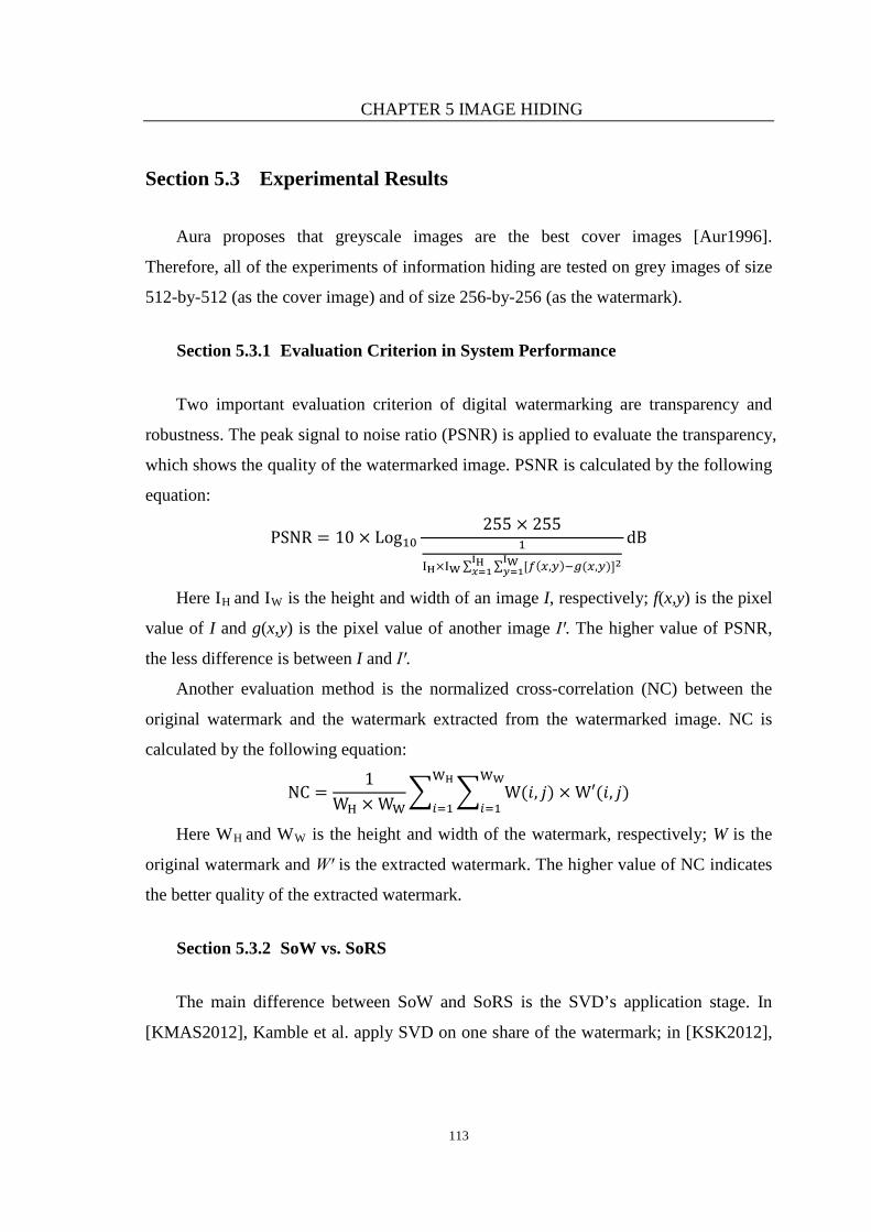
CHAPTER 5 IMAGE HIDING
113
Section 5.3 Experimental Results
Aura proposes that greyscale images are the best cover images [Aur1996].
Therefore, all of the experiments of information hiding are tested on grey images of size
512-by-512 (as the cover image) and of size 256-by-256 (as the watermark).
Section 5.3.1 Evaluation Criterion in System Performance
Two important evaluation criterion of digital watermarking are transparency and
robustness. The peak signal to noise ratio (PSNR) is applied to evaluate the transparency,
which shows the quality of the watermarked image. PSNR is calculated by the following
equation:
PSNR = 10 × Log10255 × 255
1
IH×IW ∑ ∑ [𝑓(𝑥,𝑦)−𝑔(𝑥,𝑦)]2IW𝑦=1
IH𝑥=1
dB
Here IH and IW is the height and width of an image I, respectively; f(x,y) is the pixel
value of I and g(x,y) is the pixel value of another image Iꞌ. The higher value of PSNR,
the less difference is between I and Iꞌ.
Another evaluation method is the normalized cross-correlation (NC) between the
original watermark and the watermark extracted from the watermarked image. NC is
calculated by the following equation:
NC =1
WH × WW� � W(𝑖, 𝑗) × W′(𝑖, 𝑗)
WW
𝑖=1
WH
𝑖=1
Here WH and WW is the height and width of the watermark, respectively; W is the
original watermark and Wꞌ is the extracted watermark. The higher value of NC indicates
the better quality of the extracted watermark.
Section 5.3.2 SoW vs. SoRS
The main difference between SoW and SoRS is the SVD’s application stage. In
[KMAS2012], Kamble et al. apply SVD on one share of the watermark; in [KSK2012],

CHAPTER 5 IMAGE HIDING
114
Kumar et al. perform three levels of DWT and apply SVD on the modified DWT
coefficients.
Therefore, in order to compare the algorithms, we design two algorithms based on
[KMAS2012 and KSK2012].
Section 5.3.2.1 Comparing PSNR between the Carrier Image and the Watermarked Image
Figure 5.9 shows the experimental results of the watermarked image and the
extracted watermark performed by SoW and SoRS under the embedding strength 0.002.
(1) Original Image and the Watermark
(2) Watermarked Image and the Extracted Watermark Performed by SoW

CHAPTER 5 IMAGE HIDING
115
(3) Watermarked Image and the Extracted Watermark Performed by SoRS
Figure 5.9 Watermarked Image and the Extracted Watermarked by the Two
Algorithms
Figure 5.9 indicates that the PSNR and the NC of the watermarks extracted by SoW
and SoRS are of not much difference. But the PSNR value of the watermarked image
between these two algorithms is of great difference. The conclusion can be drawn from
Table 5.1.
Table 5.1 Comparisons of PSNR between SoW and SoRS under Various
Embedding Strength α
α
PSNR 0.002 0.20 0.35 0.50 0.65 0.80 0.999
SoW 109.8408 89.8408 64.98 61.882 59.6031 57.7996 55.8701
SoRS 130.9163 90.7894 85.8049 82.582 80.1838 78.2597 76.1678
Difference 19.187% 1.056% 32.048% 33.451% 34.53% 35.398% 36.33%
Table 5.1 shows that, in all of the test cases, the PSNR of the watermarked image
performed by SoRS is higher than that of SoW. With very high embedding strength,
0.999 for example, SoRS gets 36.33% higher value of PSNR. As a result, for a better
quality of transparency of the watermarked image, SoRS is preferable.
Section 5.3.2.2 Comparing PSNR and NC between the Original Watermark and the Extracted Watermark upon Various Attacks
• JPEG compression attack:
The JPEG compression algorithm is designed to compress image files created using
the Joint Photographic Experts Group (JPEG) standard.

CHAPTER 5 IMAGE HIDING
116
Table 5.2 PSNR and NC between the Original Watermark and the Extracted Watermark
upon JPEG Compression Attack
Attacked
Image
Extracted Watermark PSNR NC
SoW SoRS SoW SoRS SoW SoRS
1
48.1308 55.6145 0.0000 0.8777
40
48.6733 61.2184 0.1835 0.9652
80
51.6574 63.9353 0.6387 0.9810
100
53.4655 70.0117 0.7593 0.9952
From Table 5.2 we see that the NC of SoRS is higher than that of SoW. SoW shows
better visual perceptibility upon strong JPEG compression attack, but with the quality

CHAPTER 5 IMAGE HIDING
117
factor of the attack getting higher, SoW cannot extract the watermark properly,
especially when the compression quality factor is 80.
• Filter attacks:
Digital filter is a system that performs mathematical operations on a signal to reduce
or enhance certain aspects of that signal.
Various filtering attacks, including Gaussian low-pass filter, average filter and
median filter, are performed to test the robustness of these two proposed algorithms.
Table 5.3 PSNR and NC between the Original Watermark and the Extracted Watermark
upon Filtering Attack
Attack Types Attacked Image
Extracted Watermark PSNR NC
SoW SoRS SoW SoRS SoW SoRS
Gaussian
Low-pass Filter
3,0.5
48.1308
62.6053
0.0000
0.9742
3,0.1
49.8408
70.9174 NaN 0.996
1
3,0.8
48.1404
58.8778
0.0047
0.9421

CHAPTER 5 IMAGE HIDING
118
10,0.5
49.4063
59.5672
0.4069
0.9500
Average Filter
3
48.2746
57.712
0.0663
0.9262
10
48.1308
57.5607
0.0000
0.9238
50
48.1308
53.2816
0.0000
0.7409
Median Filter
48.1308
58.2699
0.0000
0.9342
In Table 5.3, NaN stands for Not a Number. It indicates the extracted watermark is
nothing like the original one.

CHAPTER 5 IMAGE HIDING
119
From this table we can see that the performance of SoRS is better than that of SoW
whether in PSNR or NC. Most of the extracted watermarks performed by SoW are
negative images, but the visual perceptibility is even better than those performed by
SoRS.
In a nutshell, SoRS shows better robustness than SoW against filter attacks.
• Contrast adjustment attacks:
Contrast is determined by the difference in the colour and brightness of the image.
Table 5.4 PSNR and NC between the Original Watermark and the Extracted Watermark
upon Contrast Adjustment Attacks
Attack Types Attacked Image
Extracted Watermark PSNR NC
SoW SoRS SoW SoRS SoW SoRS
Histogram
Equalization
Inf 61.6018
1.0000
0.9683
Contrast
Increasing
0.1-0.9
Inf 69.8908
1.0000
0.9951
0.1-0.2
81.2441
55.4150
0.9996
0.8842

CHAPTER 5 IMAGE HIDING
120
0.5-0.6
89.3059
57.5508
0.9999
0.9247
0.8-0.9
48.1746
52.4435
0.0211
0.6842
Inf in this table represents infinite value, it means the extracted watermark is nearly
the same as the original one. In this test, SoW beats SoRS. Even though the NC of SoW
is much lower than that of SoRS when the contrast parameter is 0.8-0.9, from the visual
perception aspect, the extracted watermark performed on SoW is easier to perceive.
• Geometrical transform attacks:
Geometric transformation of images is a class of operations that alter the spatial
relationships between the pixels.
Table 5.5 PSNR and NC between the Original Watermark and the Extracted Watermark
upon Geometrical Transform Attacks
Attack Types Attacked Image
Extracted Watermark PSNR NC
SoW SoRS SoW SoRS SoW SoRS
Cropping
30%
49.3715
58.6718
0.3966
0.9396

CHAPTER 5 IMAGE HIDING
121
50%
48.1323
53.1162
0.0007
0.7607
80%
48.9106
52.6142
0.2859
0.7134
Rotation
30
48.6866
64.6969
0.1668
0.9840
60
49.6073
63.8976
0.3586
0.9808
90
51.1404
62.8536
0.5807
0.9756

CHAPTER 5 IMAGE HIDING
122
Circular Shift
128,128
49.8408
70.9174 NaN 0.996
1
256,256
49.8408
57.712 NaN 0.996
1
Motion Blurred
9,0
48.1308
57.0157
0.0000
0.9568
128,45
48.1308
62.0078
0.0000
0.9929
Scale
0.1
48.1308
56.0903
0.0000
0.9774

CHAPTER 5 IMAGE HIDING
123
0.5
48.1308
59.2653
0.0000
0.9030
10
48.1308
64.5725
0.0000
0.9442
Table 5.5 indicates RoRS performs nicely against most of the geometrical distortion
attacks. But SoW performs better than SoRS in cropping attack, even the NC is nearly
zero, the extracted watermark performed on SoW is easier to perceive.
• Noise addition attacks:
Image noise is random variation of brightness or colour information in images.
Gaussian noise is a standard model of amplifier noise, salt-and-pepper noise will have
dark pixels in bright regions and bright pixels in dark regions, while speckle noise in
conventional radar results from random fluctuations in the return signal from an object
that is no bigger than a single image-processing element. It increases the mean grey level
of a local area [TM2009].
Experimental results from Table 5.6 show the strong robustness of these two
proposed algorithms against noise addition attacks. But SoW slightly beats SoRS.

CHAPTER 5 IMAGE HIDING
124
Table 5.6 PSNR and NC between the Original Watermark and the Extracted Watermark
upon Noise Addition Attacks
Attack Types Attacked Image
Extracted Watermark PSNR NC
SoW SoRS SoW SoRS SoW SoRS
Gaussian Noise
0.5
Inf 67.9833
1.0000
0.9924
0.99
Inf 68.2884
1.0000
0.9929
Salt-pepper
Noise
0.5
Inf 68.6018
1.0000
0.9934
0.99
Inf 68.4210
1.0000
0.9931
Speckle Noise
0.2
Inf 68.1531
1.0000
0.9927

CHAPTER 5 IMAGE HIDING
125
0.5
Inf 68.4494
1.0000
0.9932
0.8
Inf 68.1665
1.0000
0.9927
For better comparison, we draw one graph for PNSR and another one for NC. We
replace Inf with 100 and NaN with -1.
Figure 5.10 PSNR of the Watermark Extracted from SoW and SoRS
0
20
40
60
80
100
120
SoW SoRS

CHAPTER 5 IMAGE HIDING
126
Figure 5.11 NC of the Watermark Extracted from SoW and SoRS
From Figure 5.10 and Figure 5.11, we see that compared to SoW, SoRS performs
better and shows more stability in most cases, even though SoW performs much better
than SoRS when extracting watermark from the image after noise (Gaussian noise,
salt-pepper noise, speckle noise) attacks. This discovery is an interesting and abnormal
one. We tried to find the reasons behind the experiments, only to found out it has to be
explained in mathematical way (because SVD is about the transform of matrix), but is
not actually what we focus on in the research, so we just show the experiments.
Therefore, in general, SoRS has better results of the extracted watermark because it
performs more stable against most of the attacks. Hence for a long-term and general
application, SoRS is more suitable.
Section 5.3.3 SoRS vs. Other Algorithms
In order to authenticate the performance of the proposed technique, SoRS is
compared with other competing algorithms.
0
0.2
0.4
0.6
0.8
1
1.2
SoW SoRS

CHAPTER 5 IMAGE HIDING
127
Section 5.3.3.1 SoRS vs. KMAS
We evaluated the proposed watermarking scheme, by testing on several 512-by-512
still images, see Figure 5.12. The watermark used for test can be seen in Figure 5.13.
(1) Lena (2) Couple (3) Pirate
(4) Cameraman (5)Blonde (6) Mandrill
Figure 5.12 Standard Carrier Images
Figure 5.13 Watermark used in the Experiments

CHAPTER 5 IMAGE HIDING
128
In Kamble et al.’s algorithm [KMAS2012], the PSNR, which obtained between
carrier image and watermarked image for all standard test images, has 109.5099 as the
minimum value and 109.5165 as the maximum value.
But the value of PSNR is decided by the embedding strength α. By experiment,
PSNR of the proposed algorithm can reach 73.9 if α=0.999999 and 235.4 if
α=0.00000001. Thus it is meaningless to compare PSNR obtained between KMAS’s
algorithm and the proposed one.
Therefore, the performance of the algorithms can be compared by NC between
embedded/extracted watermarks. In this case, the embedding strength of the proposed
algorithm α=0.002 with the average PSNR value around 129 on all six standard test
images.
Table 5.7 and Figure 5.14 shows the proposed algorithm is more robust against
different attacks.

CHAPTER 5 IMAGE HIDING
129
Table 5.7 Comparisons of NC between Embedded and Extracted Watermark Performed by KMAL’s Algorithm and SoRS
Image Attacks Lena Couple Pirate Cameraman Blonde Mandrill
KMAS’s SoRS KMAS’s SoRS KMAS’s SoRS KMAS’s SoRS KMAS’s SoRS KMAS’s SoRS
Cropping 0.9865 0.9891 0.9833 0.9888 0.9777 0.9876 0.9865 0.9905 0.9869 0.9918 0.9914 0.9909
Speckle Noise 0.9924 0.9979 0.9898 0.9985 0.9885 0.9979 0.9911 0.9990 0.9894 0.9981 0.9874 0.9977
Gaussian Noise 0.9885 0.9934 0.9885 0.9989 0.9860 0.9979 0.9885 0.9992 0.9864 0.9987 0.9859 0.9980
Rotation 0.9872 0.9928 0.9879 0.9975 0.9809 0.9880 0.9847 0.9976 0.9834 0.9845 0.9891 0.9921
Histogram
Equalization 0.9898 0.9937 0.9841 0.9957 0.9898 0.9952 0.9879 0.9981 0.9864 0.9936 0.9874 0.9942
Salt-Pepper Noise 0.9885 0.9972 0.9853 0.9988 0.9866 0.9973 0.9879 0.9991 0.9889 0.9984 0.9884 0.9983
Gaussian filter 0.9872 0.9879 0.9878 0.9981 0.9872 0.9902 0.9866 0.9932 0.9859 0.9925 0.9909 0.9914
Resize 0.9885 0.98594 0.9872 0.9851 0.9872 0.9814 0.9885 0.9907 0.9929 0.9826 0.9934 0.9833
MotionBlurred 0.9815 0.9877 0.8177 0.9834 0.9838 0.9864 0.9140 0.9899 0.9864 0.9984 0.8980 0.9876

CHAPTER 5 IMAGE HIDING
130
(1) Lena
(2) Couple
(3) Pirate
0.980.9820.9840.9860.988
0.990.9920.9940.9960.998
1
Cropping SpeckleNoise
GaussianNoise
Rotation HistogramEqualization
Salt-PepperNoise
Gaussianfilter
KMAS’s SoRS
0.975
0.98
0.985
0.99
0.995
1
1.005
Cropping SpeckleNoise
GaussianNoise
Rotation HistogramEqualization
Salt-PepperNoise
Gaussianfilter
KMAS’s SoRS
0.965
0.97
0.975
0.98
0.985
0.99
0.995
1
Cropping SpeckleNoise
GaussianNoise
Rotation HistogramEqualization
Salt-PepperNoise
Gaussianfilter
KMAS’s SoRS

CHAPTER 5 IMAGE HIDING
131
(4) Cameraman
(5) Blonde
(6) Mandrill
Figure 5.14 Comparison of NC between KMAS’s Algorithm and SoRS Performed on
Different Standard Carrier Images
0.975
0.98
0.985
0.99
0.995
1
1.005
Cropping SpeckleNoise
GaussianNoise
Rotation HistogramEqualization
Salt-PepperNoise
Gaussianfilter
KMAS’s SoRS
0.975
0.98
0.985
0.99
0.995
1
Cropping SpeckleNoise
GaussianNoise
Rotation HistogramEqualization
Salt-PepperNoise
Gaussianfilter
KMAS’s SoRS
0.975
0.98
0.985
0.99
0.995
1
Cropping SpeckleNoise
GaussianNoise
Rotation HistogramEqualization
Salt-PepperNoise
Gaussianfilter
KMAS’s SoRS
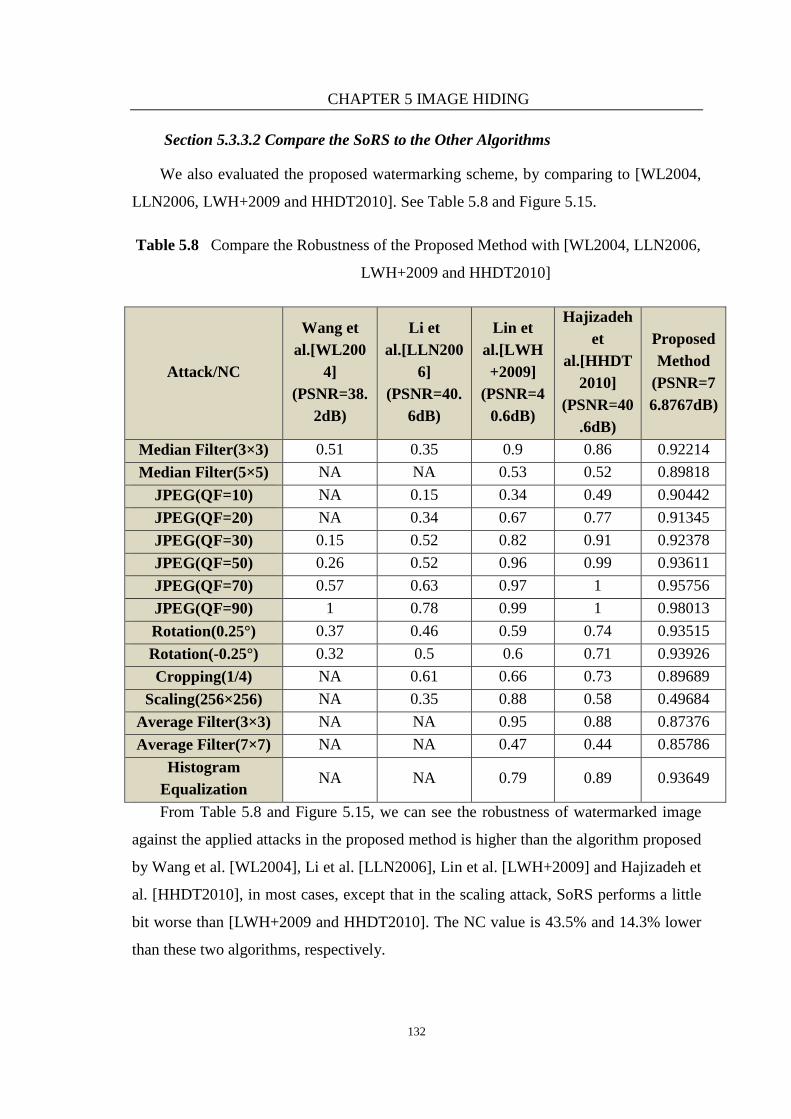
CHAPTER 5 IMAGE HIDING
132
Section 5.3.3.2 Compare the SoRS to the Other Algorithms
We also evaluated the proposed watermarking scheme, by comparing to [WL2004,
LLN2006, LWH+2009 and HHDT2010]. See Table 5.8 and Figure 5.15.
Table 5.8 Compare the Robustness of the Proposed Method with [WL2004, LLN2006,
LWH+2009 and HHDT2010]
Attack/NC
Wang et al.[WL200
4] (PSNR=38.
2dB)
Li et al.[LLN200
6] (PSNR=40.
6dB)
Lin et al.[LWH+2009]
(PSNR=40.6dB)
Hajizadeh et
al.[HHDT2010]
(PSNR=40.6dB)
Proposed Method
(PSNR=76.8767dB)
Median Filter(3×3) 0.51 0.35 0.9 0.86 0.92214 Median Filter(5×5) NA NA 0.53 0.52 0.89818
JPEG(QF=10) NA 0.15 0.34 0.49 0.90442 JPEG(QF=20) NA 0.34 0.67 0.77 0.91345 JPEG(QF=30) 0.15 0.52 0.82 0.91 0.92378 JPEG(QF=50) 0.26 0.52 0.96 0.99 0.93611 JPEG(QF=70) 0.57 0.63 0.97 1 0.95756 JPEG(QF=90) 1 0.78 0.99 1 0.98013 Rotation(0.25°) 0.37 0.46 0.59 0.74 0.93515 Rotation(-0.25°) 0.32 0.5 0.6 0.71 0.93926 Cropping(1/4) NA 0.61 0.66 0.73 0.89689
Scaling(256×256) NA 0.35 0.88 0.58 0.49684 Average Filter(3×3) NA NA 0.95 0.88 0.87376 Average Filter(7×7) NA NA 0.47 0.44 0.85786
Histogram Equalization
NA NA 0.79 0.89 0.93649
From Table 5.8 and Figure 5.15, we can see the robustness of watermarked image
against the applied attacks in the proposed method is higher than the algorithm proposed
by Wang et al. [WL2004], Li et al. [LLN2006], Lin et al. [LWH+2009] and Hajizadeh et
al. [HHDT2010], in most cases, except that in the scaling attack, SoRS performs a little
bit worse than [LWH+2009 and HHDT2010]. The NC value is 43.5% and 14.3% lower
than these two algorithms, respectively.

CHAPTER 5 IMAGE HIDING
133
Figure 5.15 Comparing the Robustness of the Proposed Method with [WL2004, LLN2006, LWH+2009 and HHDT2010]
0
0.2
0.4
0.6
0.8
1
1.2
Wang et al.[WL2004] (PSNR=38.2dB) Li et al.[LLN2006] (PSNR=40.6dB) Lin et al.[LWHK2009] (PSNR=40.6dB)
Hajizadeh et al.[HHDT2010] (PSNR=40.6dB) Proposed Method (PSNR=76.8767)

CHAPTER 5 IMAGE HIDING
134
For more comparison of the robustness of the watermark against JPEG compression,
we also compare the proposed algorithm with Hajizadeh et al. [HHDT2010] and Byun et
al. [BLK2005]. From Table 5.9 and Figure 5.16, the proposed algorithm has the most
robustness to against strong JPEG attack with quality factors 10, 20 and 30. And the NC
of the proposed algorithm is quite stable compared with the competing methods
mentioned in this chapter.
Table 5.9 Compare the NC of the Proposed Method with Hajizadeh et al. [HHDT2010]
and Byun et al. [BLK2005] after JPEG Compression
QF Byun [BLK2005] (PSNR=41.95)
Hajizadeh [HHDT2010] (PSNR=40.6dB)
Proposed Method (PSNR=76.8767)
10 0.49 0.49 0.93 20 0.6 0.77 0.94 30 0.77 0.91 0.95 40 0.81 0.99 0.95 50 0.83 0.99 0.96 60 0.9 1 0.97 70 0.94 1 0.98 80 0.97 1 0.98 90 0.99 1 0.99
100 1 1 0.99
Figure 5.16 Compare the NC of the Proposed Method with Hajizadeh et al.
[HHDT2010] and Byun et al. [BLK2005] after JPEG Compression
00.20.40.60.8
11.2
10 20 30 40 50 60 70 80 90 100
Byun[13](PSNR=41.95)
Hajizadeh et al.[HHDT2010] (PSNR=40.6dB)
Proposed Method (PSNR=76.8767)

CHAPTER 5 IMAGE HIDING
135
Section 5.4 Conclusions
In this chapter, we have proposed a hybrid digital watermarking scheme based on
DWT-SVD and ergodic matrix. The watermark has been divided into four shares and
embedded in the singular values of the carrier image’s second-level DWT.
Experimental results show that, in general, performing SVD on the singular value
revised by the watermark and the carrier image (SoRS) is better than on the singular
value of the watermark (SoW). And the experimental results also show that embedding
watermark in the high frequency subbands has more robustness over low frequency
subbands.
Compared to other watermarking schemes, SoRS has also shown both the
significant improvement in perceptibility and the robustness under various types of
image processing attacks. Even though this algorithm is weak against scaling attacks, it
extracts watermarks of higher quality than other algorithms under many attacks such as
JPEG compression, filtering, histogram equalization, rotation, cropping and noise. As a
whole, the proposed method is a useful tool for ownership identification and copyright
protection.

CHAPTER 6 TEMPORAL APPLICATIONS
136
CHAPTER 6 TEMPORAL
APPLICATIONS
Temporal Logic has been existing for more than a half century, it has so many
applications in the variety fields, but in information security field, it has only been
applied in protocol so far. However, actually, there is such a relation between temporal
logic and information encryption/hiding.
Section 6.1 Formal Characterization of Time-series
Section 6.1.1 Why Choosing Temporal
The term Temporal Logic is a special branch of modal logic. It is largely used to
describe systems of symbolism and rules for representing, and reasoning about,
propositions qualified in terms of time. It is also more specifically refer to Tense Logic,
a modal logic-based system of temporal logic introduced in the 1960s by Arthur Prior
and subsequently developed further by logicians and computer scientists, particularly
Amir Pnueli [DEJ+2007], he suggested using Linear-Time Propositional Temporal
Logic (LTL) to reason about concurrent programs. Temporal logics include interval
temporal logic (ITL) and μ calculus. ITL offers flexible specification and proof
techniques for reasoning about properties involving safety, liveness and projected time
[MWH2002]. Modal μ calculus is an extension of propositional modal logic with a least
fixed point (LFP, the least fixed point is less than or equal to all other fixed points
according to some partial order) operator μ. It can be described and verified properties of
labelled transition systems [LH2007].
Temporal logic can be applied to/in:
• Natural language. Prior, the founding father of temporal logic, lists the
precursors of Tense Logic in [MBZ2008]. One of them is Hans Reichenbach. He

CHAPTER 6 TEMPORAL APPLICATIONS
137
analysed the tenses of English and put forward that the function of each tense is to
specify the temporal relationships amongst a set of three times related to the utterance,
specifically S (the speech time), R (the reference time) and E (the event time). Prior
points out that Reichenbach’s analyses are insufficient to explain the full range of tense
usage in natural language. Consequently much work has been done to refine the analysis
of tenses and other temporal expressions in language such as the temporal prepositions
and connectives (“before”, “after”, “since”, “during”, “until”), using the many varieties
of temporal logic.
• Artificial intelligence. It is often associated with the work of Allen, which is
concerned with how to find a general framework for all the temporal representations
required by AI programs [All1984]. A useful survey of issues involving time and
temporal reasoning in AI is Galton [MK1994], and a comprehensive coverage of the
area is summarized by Fisher et al. [Bee1992] in their handbook in 2005. Much of the
work on temporal reasoning in AI has been closely related to the notorious frame
problem, which is concerned with formalising the logic of actions and events in such a
way that many inferences of this kind are indefinitely made available without our having
to encode them all unambiguously.
• Computing science. Temporal logic is given an intensive application in this
specific area by Pnueli in [DEJ+2007]. It is concentrated on the specification and
verification of programs, especially during the multi-tasking of applications concurrently
being processed by the computer. In order to make sure that such a program behaves
correctly, it is essential to specify the way in which the actions of the various processors
are interrelated. The relative timing of the actions must be cautiously coordinated so that
integrity of the information shared among the processors can be surely maintained.
Non-determinism is an essential concern in computer science applications. There are two
important systems for temporal logic namely, CTL or Computation Tree Logic and the
more expressive CTL System.
It is easy to notice that, there is no such a relation between temporal logic and
cryptography/hiding even though temporal logic has so many applications in the variety

CHAPTER 6 TEMPORAL APPLICATIONS
138
fields. However, in a communication, one party may possibly send a series of
information to the other at different time or in different order.
Since temporal logic, especially temporal order theory, deals with time series data,
we shall apply it in cryptography and information hiding. From the results of CHAPTER
4 and of CHAPTER 5, we take image security as a special case, to analyse how to
realize this goal.
Section 6.1.2 Formalize the Characterization of Time-series
As mentioned in the Section 1.1.1, in most literature in the domain of data mining,
the fundamental time theories based on which time-series and sequences are formed up
are usually not explicitly specified. However, no matter what a time theory or model is
chosen, a temporal order representing the “Immediately Before” relationship is needed
for defining time-series.
In a system based solely on intervals as primitive like that of Allen’s interval
temporal theory [All1984], or a system based on both points and intervals like that of Ma
and Knight [MK1994], such an immediately before relation can be directly expressed by
the “Meets” relation.
N.B. The intuitive meaning of Meets(t1, t2) is that, on the one hand, t1 and t2 don’t
overlap each other (i.e., they don’t have any part in common, not even a point); on the
other hand, there is not any other time object standing between them.
As shown in [MH2006], the two different approaches to the treatment of intervals,
i.e., taking intervals as primitive or as derived objects constructed out of primitive points,
are actually reducible to logically equivalent expressions under some requisite
interpretations. In fact, in a system based solely on points as primitive, say (P, ≤), as the
derived objects, an interval can be defined as a typed (left-open & right-open, left-closed
& right-open, left-open & right-closed, left-closed & right-closed) subset of the set of
primitive points, which must be in one of the following four forms:
(p1, p2) = {p | p∈P ˄ p1<p<p2} [p1, p2) = {p | p∈P ˄ p1≤p<p2}

CHAPTER 6 TEMPORAL APPLICATIONS
139
(p1, p2] = {p | p∈P ˄ p1<p≤p2} [p1, p2] = {p | p∈P ˄ p1≤p≤p2}
where p1<p2 ⇔ p≤p2 ˄ ¬(p1 = p2)
Without confusion, an interval with the special form of [p, p] is simply taken as
identical to point p.
In the same manner as the approach that treats intervals as primitive, an
immediately before relation, “Meets”, can be defined over typed-point-based intervals as
below:
Meets(t1, t2) ⇔∃p1,p,p2∈P(t1 = (p1, p) ∧t2 = [p, p2)
∨t1 = [p1, p) ∧t2 = [p, p2)) ∨t1 = (p1, p) ∧t2 = [p, p2]
∨t1 = [p1, p) ∧t2 = [p, p2] ∨t1 = (p1, p] ∧t2 = (p, p2)
∨t1 = [p1, p] ∧t2 = (p, p2) ∨t1 = (p1, p] ∧t2 = (p, p2]
∨t1 = [p1, p] ∧t2 = (p, p2])
Analogously, the 13 relations introduced by Allen for primitive intervals [All1984],
including “Equal”, “Before”, “After”, “Meets”, “Met-by”, “Overlaps”, “Overlapped-by”,
“Starts”, “Starts-by”, “During”, “Contains”, “Finishes” and “Finished-by”, can also be
defined in terms of the above single relation “Meets”.
From the definition, for any two typed-point-based intervals t1 and t2 such that
Meets(t1, t2), there is a unique time interval corresponds to the ordered union of t1 and
t2.. By axiomatization, this also applies to systems that based solely on intervals as
primitive or based on both points and intervals as primitive. Therefore, in the case
Meets(t1, t2), the unique ordered union of t1 and t2 can be denoted as t1⊕t2.
In a time model based solely on points as primitive, the collection of time-elements
is defined as the minimal set closed under the following rules:
Each primitive point is a time-element;
Each derived typed-point-based interval is a time-element;

CHAPTER 6 TEMPORAL APPLICATIONS
140
If t1 and t2 are two time-elements and Meets(t1, t2), then the unique ordered
union, t1⊕t2 is a time-element.
Similarly, in a time model based on both points and intervals as primitive, the
collection of time-elements is defined as the minimal set closed under the following
rules:
Each primitive point and/or interval is a time-element;
If t1 and t2 are time-elements and Meets(t1, t2), then the unique ordered union,
t1⊕t2 is a time-element.
Within a temporal framework based on a chosen time theory (either point-based,
interval-based, or point&interval-based), a time-series ts is defined as a vector of
time-elements temporally ordered one after another. Formally, a general time-series
(GTS) is a triple (ts, R, Dur) which is defined in terms of the following schema:
GTS 6.1) ts = [t1, …, tn]
GTS 6.2) R=Meets(tj, tj+1) ∨ Before(tj, tj+1), for all j = 1, …, n-1
GTS 6.3) Dur(tk) = dk, for some k where 1≤ k ≤ n and di is a non-negative real
number.
where Before(t1, t2) ∃t(Meets(t1, t) ∧ Meets(t, t2)).
Generally speaking, a time-series may be incomplete in various ways. For example,
if the relation between tj and tj+1 is “Before” rather than “Meets”, it means that the
knowledge about the time-element(s) between tj and tj+1 is not available. In addition, if
Dur(tk) = dk is missing for some k, it means that duration knowledge as for time-element
tk is unknown. Correspondingly, a complete time-series (CTS) is defined in terms of the
schema as below:
CTS 6.1) ts = [t1, …, tn]
CTS 6.2) Meets(tj, tj+1), for all j = 1, …, n-1
CTS 6.3) Dur(ti) = di, for all i = 1, …, n, where di is a non-negative real number.

CHAPTER 6 TEMPORAL APPLICATIONS
141
Section 6.2 Temporal-based Image Cryptosystem
Given Alice sends Bob a sequence of images Img1, Img2, …, Imgn, next time she
might send the same sequence with different order such as Img2, Img1, …, Imgn. What
she can do if the importance of each image changes? How can she change the encryption
results with diverse order of the images to avoid suspicion? Nevertheless, according to
the author’s knowledge, such consideration hasn’t been included in state-of-the-art
cryptosystems, much less in image cryptosystems.
As a result, this section tries to answer the following two questions:
Question6.2.1: How can Alice encrypt different important-level images without
changing the keys?
Question6.2.2: How can Alice get different encryption results if the order of the
images is changed?
Section 6.2.1 Encryption-decryption Process Using Temporal Logic
To solve two questions listed above, we shall apply temporal logic in our
cryptosystem. The basic thoughts are as follows:
(1) The temporal-based image series is defined as a vector of time-elements
temporally ordered one after another.
(2) Take each image as a node, draw the directed graph G.
(3) The k-th cipher image is utilized to encrypt its tail-node image (i.e. the k+1-th
image).
(4) To ensure the k-th image can be decrypted, each tail-node image can have one
and only one head-node image.
Given the cipher keys Ka, Kb and Kc, Ka are all matrices of size n×n. Alice is the
sender and Bob is the receiver. Then for Alice, she carries out the encryption process as

CHAPTER 6 TEMPORAL APPLICATIONS
142
below:
① Load image series [Img1, Img2, …, Imgn]. The order of the series can be set by
the important level of the images. The image with the lowest importance is the first node,
while the image with the highest importance is the last node;
② Draw a directed graph of the image series, and set the corresponding adjacency
matrix A;
③ E(Img1, Ka) returns the cipher-image Img1 encrypted by the key Ka, only the
first image is encrypted by Ka;
④ If [Imgk+1, …, Imgk+m] are the tail-nodes of Imgk, then diffuse each image of
tail-nodes by the key Ka, namely [E(Imgk+1, Ka), …, E(Imgk+m, Ka)]. Therefore, the
histogram of the images (even the pure-colour images) is more equalized. This step is to
enhance the encryption effects;
⑤ Encrypt each tail-nodes by its head-node, i.e., [E(E(Imgk+1, Ka), Imgk), …,
E(E(Imgk+m, Ka), Imgk)];
⑥ Go to ④ unless all the images are encrypted;
⑦ Permute the cipher image series S=[E(Img1, Ka), E(E(Imgk+1, Ka), Imgk), …,
E(E(Imgk+m, Ka), Imgk), …] by Kb, i.e., P(S, Kb). And encrypt the adjacency matrix A
by Kc, i.e.,E(A, Kc);
⑧ Send the encrypted adjacency matrix Aꞌ and the permuted series to Bob.
When Bob receives the series and Aꞌ, he decrypts the images by the following steps:
① Deduce A by Ka, i.e., D(E(Aꞌ, Kc), Kc) = A;
② Get the original order of the series by Kb, i.e., DP(P(S, Kb), Kb) = S;
③ Decrypt the first image by Ka, i.e., D(E(Img1, Ka), Ka) = Img1;

CHAPTER 6 TEMPORAL APPLICATIONS
143
④ Decrypt the tail-nodes images by its head-node image Imgk, i.e.,D(E(E(Imgk+1,
Ka), Imgk)) = E(Imgk+1, Ka);
⑤ Decrypt the image k+1 by the key Ka, i.e., D(E(Imgk+1, Ka), Ka) = Imgk+1;
⑥ Go to ④ unless all the images are decrypted.
Section 6.2.2 Expand the Key Size
If the size of Ka is smaller than that of the image, Alice expands Ka according to the
first encrypted image by the following algorithm:
① H and W is respectively the height and width of the first encrypted image;
② N is the number of the elements of Ka;
③ R rounds the elements of H×W/N to the nearest integers greater than or equal to
H×W/N;
④ ArrayB stores the result of R matrices that Alice calculates;
⑤ for i=1 to R
⑥ the i-th row of ArrayB stores the result of Power(Ka,Ka(i));
⑦ endfor
Then ArrayB is the actually what Alice uses to encrypt the image.
Section 6.2.3 Adjust the Images
In an temporal-based image system, each image in the series [Img1, Img2, …,
Imgn], for example Imgk, could be a “key” to encrypt the next image Imgk+1. The
encryption algorithm can be the same as what we described in Section 4.2 when Img1 is
encrypted by the session key Ka.

CHAPTER 6 TEMPORAL APPLICATIONS
144
Noted that the size of the images are not necessarily equal to each other, we need to
adjust the images so that it can be used to encrypt the next one(s). Such algorithm can be
described as follows:
①Ceil(A) rounds the elements of A to the nearest integers greater than or equal to A;
Sqrt(A) returns the square root of A;
Size(A) returns the size of the matrix A;
②n = size(Imgk) – size(Imgk+1);
③if n> 0, delete the last n elements from Imgk;
④else if n≤0 do the following:
⑤ m=ceil(sqrt(ceil(size(Imgk+1)/size(Imgk))));
⑥for k=1:m
⑦form a new matrix Imgk' such that the weight and the height of it equals to
size(Imgk+1);
⑧end for
⑨delete the last n elements from Imgk ' such n = size(Imgk') – size(Imgk+1);
Section 6.2.4 Security Analysis
A good encryption system shall resist all kinds of known attacks, including
ciphertext-only attack, know-plaintext attack, statistical attack, and various brute-force
attacks. Thus in what follows, we will analyse on the proposed image encryption scheme,
including the most important ones such as key space analysis and statistical analysis,
which demonstrates the satisfactory security of the proposed scheme.

CHAPTER 6 TEMPORAL APPLICATIONS
145
Before security analysis, three original images, which are utilized in the
experiments, are provided in Figure 6.1.
(1) Original Lena Image (of Size 512×512)
(2) Original All-white Image (of Size 320×240)
(3) Original All-black Image (of Size 214×131)
Figure 6.1 Three Images and Their Corresponding Histograms
We randomly pick three images: Lena image, all-white image and all-black image.
Let these images be denoted as A, B, C, respectively. We apply the encryption algorithm
proposed in [Bru1972] and the temporal-based encryption algorithm in this cryptosystem.

CHAPTER 6 TEMPORAL APPLICATIONS
146
Then the encryption result can be seen from Figure 6.2.
(1) Encryption Sequence Is ABC
(2) Encryption Sequence Is CAB
Figure 6.2 Encryption Results with Different Images Sequence
0 100 2000
1000
2000
0 100 2000
500
0 100 2000
100
200
0 100 2000
100
200
0 100 2000
1000
2000
0 100 2000
500
(1.1) Encrypted A and the Corresponding Histogram
(1.2) Encrypted B and the Corresponding Histogram
(1.3) Encrypted C and the Corresponding Histogram
(2.1) Encrypted C and the Corresponding Histogram
(2.2) Encrypted A and the Corresponding Histogram
(2.3) Encrypted B and the Corresponding Histogram

CHAPTER 6 TEMPORAL APPLICATIONS
147
We can see from Figure 6.2 that the cipher images disorganize the plain-images as
much as possible so that they are hard to recognize. And the histogram is fairly uniform
and does not reveal any statistical information of the corresponding plain-image.
Section 6.2.4.1 Key Space Analysis
Aimed at Problem 6.2.1, the key space of a good temporal-based image encryption
system shall not only be large enough to make brute-force attacks infeasible, but also
can encrypt images of different importance without changing the keys.
The algorithms used to encrypt the images can be referred to [Bru1972, Fri1998,
CM2004, MC2004, ZLW2005, GHG2005, AP2009, Moh2009, GBB+2009 and
YWL+2010]. Suppose the secret key Ka has spc different combinations, then for the
encryption systems in these algorithms, the key space is always the same if each image
is encrypted independently. However, in a temporal-based image encryption system, a
head-node image can be taken as a key for the tail-node images, namely a tail-node
image can be encrypted by its head-node image. Therefore, the probability is different
because of working out the images not only relies on the session keys but also on the
head-node image. Even an eavesdropper knows the key Ka, it is still hard for him to get
the exact order of the images without Kb and Kc.
Therefore, in the proposed temporal-based image encryption system, the key space
is Ka ×Kb × Kc.
Section6.2.4.2 Statistical Analysis
Statistical analysis is shown, in this section, by a test on the histograms of the
enciphered images and the cipher image, and on the correlations of adjacent pixels in the
two ciphered images encrypted from the same original image with the same key while in
different sequences (i.e. the head-node is different).
(1) Histogram of the plain-image and the cipher-image
Figure 6.2 shows that the histogram of each image is fairly uniform and does not
reveal any statistical information of the original image.

CHAPTER 6 TEMPORAL APPLICATIONS
148
(2) Correlation of two adjacent pixels
The experiment was divided into 10 groups, each group has 10,000 pairs of pixels,
i.e., R=10,000. The correlation distributions of two adjacent pixels in the cipher-image
are tested randomly in horizontal, vertical and diagonal. Table 6.1 shows the results of
the correlation coefficients of the cipher images using different images as their
head-note:
Table 6.1 Correlation Coefficients of Two Adjacent Pixels in the Cipher-image
B A C A A B C B A C B C
0.007334 -0.01572 -0.01689 -0.00813 0.015068 -0.01082
0.007585 -0.00642 -0.00408 -0.00315 -0.01026 0.008444
-0.01344 0.010856 -0.01093 -0.00747 0.006084 0.003443
-0.00615 0.006587 -0.00548 0.00245 -0.00153 0.014232
0.003614 0.008215 -0.01892 0.011897 -0.00812 -0.00719
0.014298 0.005353 -0.009 -0.00049 0.003064 0.009228
0.00893 0.009849 0.006174 0.010911 -0.00302 -0.00264
7.18E-05 -0.00621 -0.00674 0.011962 0.018025 0.011177
0.001893 0.004651 0.015908 -0.00019 -0.0067 3.17E-03
0.012082 -0.01394 -0.02577 -0.00468 0.003624 0.01623
Here the denotation A C means the correlation coefficients of C using E(A, Ka)
as a key. It is the same to the rest of the denotations.
We also test on various images to compare the results, see Figure 6.3 and Table 6.2.
Image (1) of Figure 6.3 is the original image and (2)-(8) are the images as keys to
encrypt (1). Table 6.2 shows that with different images and the same key Ka, the
correlation coefficients of two adjacent pixels in the cipher-image diverse.

CHAPTER 6 TEMPORAL APPLICATIONS
149
(1) Lena (2) Blonde (3) Hill (4) Man
(5) Couple (6) House (7) Pentagon (8) Peppers
Figure 6.3 Original Image (Image (1)) and the Images used as Keys (Image (2)-(8))
Table 6.2 Correlation Coefficients of Two Adjacent Pixels in the Cipher-image
Blonde Hill Man Couple House Pentagon Peppers
Correlation values 0.0011 0.0108 -0.0069 -0.0018 0.0313 0.0011 -0.0033
It is easy to see that the all the results of correlation coefficients are quite close to 0.
This indicates that our scheme has effectively removed the correlation of adjacent pixels
in the plain-image.
Section6.2.4.3 Sensitivity-based Attack
The temporal-based image encryption algorithm shall be robust enough to resist
sensitivity-based attack. This means if the order of the image series changes, it will
cause a great difference in the cipher-images, or else the temporal theory would be
utterly meaningless in this thesis.

CHAPTER 6 TEMPORAL APPLICATIONS
150
The sensitivity of the cryptosystem is largely infected not by the keys that Alice and
Bob are holding (read [YWL+2010] for reference), but also by the order of the image
series. Here, two common measures are used to test the system: NPCR and UACI.
For more evidence, we used the same formula (4.4) given in Section 4.3.2.2, except
that in this test, we compare the values of corresponding pixels in the two cipher-images.
The values of NPCR, UACI and COV (Covariance) for the cipher-image using
different images as keys are listed in Table 6.3.
Table 6.3 NPCR and UACI of the Cipher-image using Different Images as Keys
This table indicates that in a temporal ordered cryptosystem, the results of the
ciphered images are quite different even they are from the same image and encrypted by
the same key.
Section 6.3 Temporal-based Image Hiding
With more applications of information hiding, especially watermarking, various
techniques are introduced, such as fragile watermarking and robust watermarking. For
the reason that different watermarking techniques showing at different stages with
different purposes, therefore, a new technique, called multiple digital watermarking, is
introduced by other scientists [GPK2005, Lee2009 and HHLL2009].
The multiple digital watermarking techniques are for fixing the problems of the
copyright certification of a digital product produced by multiple authors when it is
released, sold and used. Compared to single watermarking techniques, embedding
multiple watermarks is more complicated. It requires the watermark signals shall not
Encryption Sequence NPCR UACI COV
B A and C A 0.996025 0.334778 -0.00055453
A B and C B 0.996068 0.334648 -0.0017352
A C and B C 0.995898 0.336168 -0.0057025

CHAPTER 6 TEMPORAL APPLICATIONS
151
interfere with each other through the embedding and the detecting procedure. Therefore,
the balance between watermark transparency and robustness is a tough issue.
Multiple digital watermarking can be classified into two categories, i.e., static
multiple digital watermarking and dynamic multiple digital watermarking.
Section 6.3.1 Static Multiple Digital Watermarking with Temporal Logic
Static multiple digital watermarking techniques are simple. Various watermarks can
be jointed into one larger watermark according to some certain rules. For example, if all
the authors create the product simultaneously, multiple watermarks can be sorted
according to the contributions of the authors. See Figure 6.4 for an example.
(1) Greenwich (2) Cambridge (3) Harvard (4) Oxford
(5) Watermark Jointed According to Alphabet
(6) Watermark Jointed According to University Founding year
Figure 6.4 Multiple Watermarks and the Joint Watermark
Considered the limited capacity of the carrier image, multiple watermarks shall not
be simply jointed by putting them together. Other issues, such as image compression or
re-encoding images to decrease the image size, shall be considered. But this is not what

CHAPTER 6 TEMPORAL APPLICATIONS
152
we shall discuss in this thesis, for we only need to focus on the techniques of watermark
embedding and extracting.
Once multiple watermarks are integrated into one, the watermarking scheme
proposed in CHAPTER 5 can be used in static multiple digital watermarking system.
Section 6.3.2 Dynamic Multiple Digital Watermarking Considering Temporal
Logic
Although lots of work has been done in the field of watermarking [BYK1998 and
TWZ2006], little specific work is done in the area of “dynamic multiple digital
watermarking”. By the time we are writing this thesis, we have only found one paper
(which is written by Tang et al. [TWZ2006]), is on this topic. Other papers discussing
“dynamic multiple watermarking” actually reflect in the embedding/extracting process
[GPK2005, TX2008, Lee2009, HHLL2009 and ZYLC2012], rather than in the
collaborating digital products considering temporal issue in an open network. How to
design watermarks created by different authors at different time? – This is what we need
to discuss in this section.
Section 6.3.2.1 How Problems Occur
In a procedure of designing a digital product, especially of collaborating on a
product through network protocol, there are often multiple authors. However, not every
author designs the product at the same time - this makes it difficult for one taking into
account at the start of a product design that:
(1) Who will collaborate on the product design?
(2) What is the number of the authors?
In the highly developed network of today, it is very common that multiple authors
cooperating on a digital product even they don’t know each other. With the improvement
of the work, the number of the authors may also be increasing because such authors are
not a team; they work independently and as an individual. As a result, in order to protect

CHAPTER 6 TEMPORAL APPLICATIONS
153
the copyrights of the authors, each identity of the author shall be designed into one
watermark and be embedded into the digital products.
It is easy to notice that, at a certain time, even when the digital product has been
released on the network, all the validated watermarks have been embedded in the
product by then. But it is not possible to predict in advance whether other watermarks, or
which watermark, will be embedded. This is a common problem of dynamic multiple
digital watermarking: We cannot predict how many watermarks will be embedded in a
digital product.
Therefore, with temporal logic theory, we set parameters as follows:
(1) Denote the digital product as DP;
(2) The number of the collaborative authors is Ni at time Ti;
(3) Denote the collaborative authors as 𝐴1𝑖 ,𝐴2𝑖 , … ,𝐴𝑁𝑖𝑖 at time Ti;
(4) Consequently, the number of the watermarks is also Ni. Denote the watermark
𝑊1𝑖,𝑊2
𝑖 , … ,𝑊𝑁𝑖𝑖 for the authors 𝐴1𝑖 ,𝐴2𝑖 , … ,𝐴𝑁𝑖
𝑖 , respectively;
(5) The version of the product DP released at time Ti is denoted as DPi; and
(6) The single joint watermark for co-authors 𝐴1𝑖 ,𝐴2𝑖 , … ,𝐴𝑁𝑖𝑖 is denoted as Wi.
With these parameters, it is obvious that, every time an author takes part in the
product design, one more watermark will need to be embedded in the product. But since
every product has its volume limitation, we cannot embed countless number of
watermarks over time. As a result, Question 6.3.1 will occur when we design a multiple
digital watermarking technique:
Question6.3.1: How to overcome the contradiction between the limitation of the
image volume and the countless number of watermarks trying to be embedded in?
According to what has been analysed in CHAPTER 5, we decide to solve the

CHAPTER 6 TEMPORAL APPLICATIONS
154
problem by embedding only one watermark regardless how many watermarks there will
be during the product design process.
However, other questions will occur that force us to face them:
Question6.3.2: Who will map the multiple watermarks to a single watermark? And
who will embed it into the image?
Question6.3.3: How to design such single watermark so that it contains the
information of the previous authors as well as the author(s) who will participate in the
product?
Question6.3.4: How to design such single watermark without revealing the plain
information of the authors to those who are going to design the watermark?
Question6.3.5: How to ensure each author that his own watermark has been
embedded into the image?
Tang proposed their method in [TWZ2006], but there are some problems lie in it:
Problem 6.3.1: Tang hasn’t considered the situation that the current authors may
collaborate on the digital product based on multiple previous products. i.e., Tang’s
model can be ascribed by Figure 6.5 (1), while ours can be ascribed by Figure 6.5 (2).
(1) Tang’s Model (2) Our Model
Figure 6.5 Model Comparision between Tang’s Method and Ours
Problem 6.3.2: The digital product may be produced based on multiple products
(different versions of the same product are regarded as different product as well), thus,
Ai
Ak
DPi Aj DPi Ai
Aj
Ak DPj
DPk

CHAPTER 6 TEMPORAL APPLICATIONS
155
how to generate the watermark for the new product? Who is responsible for embedding
the watermark?
Therefore, combine with ergodic-matrix based zero-knowledge protocol, we
propose a scheme to realize dynamic multiple digital watermarking technique to
improve Tang’s method, as well as to solve the problems we proposed.
Section 6.3.2.2 Basic Idea of the Proposed Scheme
At the time Ti when the watermark Wi is about to be inserted in the product DPi-1,
the watermark Wi-1, which has been embedded in DPi-1, shall be able to authenticate the
copyright of all the previous authors. A collaborated digital product work, considers
temporal issues (i.e., which work comes first and which comes next), can be drawn into
a directed graph as the form shown in Figure 6.6:
Figure 6.6 Directed Graph Describing a Collaborated Digital Product Work
The graph is acyclic and unweighted for two reasons:
(1) A new version of the product is generated based on the previous one(s);
(2) Authentication of the product’s authors is the main concern, thus the interval
time of the two products will not affect the watermarks.
Therefore, the graph shall be a DAG (directed acyclic graph) without weight. Such
graph, if only from the view of a new version of DP, can be classified into two scenarios,
as shown in Figure 6.7:
DP1
DP2
DP3
DP5
DP6
DP7
DP8 DP4
DP9

CHAPTER 6 TEMPORAL APPLICATIONS
156
(1) One New DP Is based on Multiple DPs (2) One New DP Is based on a Single DP
Figure 6.7 Two Scenarios of a Collaborated DP Work
For Problem 6.3.1, there’s only one watermark to embed in the product regardless
how many authors are collaborating. Considering the host image’s volume and the
algorithm complexity, we shall firstly map the multiple watermarks to a single one and
then embed it into the host image. Therefore, from the view of the authors who are going
to design a new product, there is only one scenario, which is (2) in Figure 6.7. Thus,
what we need to concern about is to prevent malicious authors cheating in the watermark.
This can be solved by a multi-secret sharing authentication scheme proposed by Wang et
al. in [WQ2006]: In the (t, n) secret sharing scheme, a dealer splits a secret into n shares
and sends a share to each of n participants. The secret message can be recovered by no
less than t members by using a publicly specified algorithm. .
After the watermark design, we can apply authentication protocols to identify the
ownership of the previous version product and embed watermark with the safe duplex
computing protocol [TWZ2006].
For Problem 6.3.2 (see (1) in Figure 6.7 for reference), the new product is based on
the existing products, and each existing product is independent from each other. As a
result, it is not appropriate for any of the authors of the existing products to embed the
watermark. Therefore, we decide to let the author of the new product to do this work. In
this case, there will be various watermarks generated from the new author and any
previous author. Hence, we convert the problem to how to integrate static multiple
watermarks into one.
DPi DPk
DPi
DPk
DPi+j
DPi+1
…

CHAPTER 6 TEMPORAL APPLICATIONS
157
The identification procedure which Bob identifies whether Alice is the true author
is realized by zero-knowledge protocol. The procedure of embedding/extracting
watermark can be referred to the algorithms proposed in CHAPTER 5.
Section 6.3.2.3 Identify the Product’s Ownership by Zero-Knowledge Protocol Based on Ergodic Matrix
Zero-knowledge protocol is a method for one party to prove to another that a
statement (usually a mathematical one) is true, without revealing anything other than the
genuineness of the statement [BFS1988].
Given Alice is the author of DP1 at time T1, Bob is the author at time T2 (T2>T1).
Before Bob decides to work on DP1, he needs to identify whether DP1 is the genuine
product. In other words, he needs to know if Alice is truly the author of DP1. Because
Bob doesn’t want to be a partner of pirates – he has to take up the responsibility of
piracy and may have to face prosecution, and also, he might not get paid for the product
design.
On the other hand, Alice wishes to protect her copyright through the identification
procedure, so that Bob will not be able to cheat when producing the joint watermark (if
Bob does, Alice still holds the fact that Bob admits she is the true author and then sues
him). But in a certain case, such as visual watermark, Alice doesn’t want to reveal too
much detail of her own watermark Wa. Once the watermark is public, anyone can easily
remove the watermark from the host image.
For all the above reasons, we introduce zero-knowledge protocol to prove Alice is
the author of DP1.
(1) Zero-knowledge Protocol Scheme 1:
Registration Process
①Alice sends the personal identification IDa to Bob for the request of registration;
②Bob searches the registration database. If IDa exists, he returns a message to

CHAPTER 6 TEMPORAL APPLICATIONS
158
Alice regarding the registration failure. Otherwise he picks an ergodic matrix Q over
finite field 𝔽𝑞 and sends it to Alice;
③Alice computes PWDa=Qa (a is Alice’s private key). Then she sends (IDa,
PWDa) to Bob.
④Bob sets up a new record for Alice in the registration database, and save (IDa,
PWDa, Q). Thus Alice successfully registers.
Identification Process
①If Alice needs to be identified by Bob, she sends IDa to Bob.
②Bob check records of Alice’s ID in the registration database. If it exists, he will
pick an integer s and sends Qs to Alice.
③Alice computes PWDa ' = (Qs )a and sends PWDa ' to Bob.
④Bob then computes PWDa '' = (PWDa)s= (Qa)s and compares PWDa ' with PWDa'',
if they matches, Alice is successfully identified.
Security Analysis
Ciphertext attack: The attacker intercepts PWDa and Q, and he wants to get Alice’s
private key a with PWDa = Qa. But since the order of Q(Q∈𝔽𝑛×𝑛𝑞 ) is qn-1, which means
the private keys a and s are in the range from 0 to qn-1. Therefore, if q and n are properly
set, a and s can be fairly large so that to get a from Qa is as hard as breaking the discrete
logarithm problem.
Disguise attack: The attacker intercepts Alice’s identification IDa, he then disguises
as Alice. But since a is Alice’s private key and the key space is quite large, he cannot
deduce PWDa, thus he is unable to be identified by Bob.
Resending attack: The attacker intercepts all the information exchanged in an
identification process. He then resends the outdated information in order to disguise

CHAPTER 6 TEMPORAL APPLICATIONS
159
himself as Alice or Bob. But this kind of attack is based on query/response, the
identification information changes each time when Alice and Bob communicate.
Therefore, the attack fails when the attacker resend PWDa ' = (Qs)a. Because Bob’s
private key s is a random number, it changes in each identification process. Thus the
attack will be found when Bob compares PWDa ' with PWDa ''.
Replacement attack: This is the most threatening attack. The attacker intercepts
(IDa, PWDa) when Alice is registering. He then replace Alice’s information with his
(IDatt, PWDatt), and logs in as Alice. Thus he can tamper with or intercept the content of
the communication between Alice and Bob.
Replacement attack can succeed because Alice’s ID is public, which gives the
attacker a good opportunity to replace Alice’s legal information in registration database.
To prevent this attack we propose the other scheme.
(2) Zero-knowledge Protocol Scheme 2–Advanced Version:
In this advanced version, Alice will encrypt her ID with a private key to prevent the
replacement attack.
Registration Process
①Alice requests identification with Bob. Bob then picks an ergodic matrix Q over
finite field 𝔽𝑞 and sends it to Alice;
②Alice encrypts her information by computing IDaa=Qaa and PWDa = Qa, then he
sends (IDaa, PWDa) to Bob.
③Bob searches the registration database. If IDaa exists, he will return a message to
Alice regarding the failed registration. Otherwise he will create a new record for Alice in
the registration database, and will store (IDaa, PWDa, Q). Thus Alice successfully
registers.
Identification Process

CHAPTER 6 TEMPORAL APPLICATIONS
160
①If Alice needs to be identified by Bob, she sends IDaa to Bob.
②Bob checks Alice’s ID record in the registration database. If it exists, he will
randomly pick an integer s and sends Qs to Alice.
③Alice computes IDaa ' = (Qs )aa and sends IDaa ' to Bob.
④Bob then computes IDaa ''=(IDaa)s= (Qaa)s and compares IDaa ' with IDaa ''.
⑤If they match, Bob will further identify Alice’s password PWDa. This process
can refer to Scheme 1.
It is obvious that Scheme 2 is more secure than Scheme 1.Because compared to
Scheme 1, Scheme 2 needs two identifications, i.e., the ID and the password of Alice. To
enhance security, Bob can send different ergodic matrices Q to Alice.
Moreover, Scheme 2 solves the security problem in Scheme 1. This scheme can
resist replacement attack, because in this scheme, Alice encrypts her ID by IDaa=Qaa ,
rather than putting it in public without any security protection.
Section 6.3.2.4 Joint Watermark Generation
Joint watermark can be generated by a trusted institution, and can also be generated
by the communication parties. The former technique is easier to realize: To achieve the
joint watermark, Alice and Bob send their watermarks to a trusted institution, then the
institution produces a watermark according to the features of Alice and Bob’s
watermarks, such as by the formula (6.1):
�𝑊𝑐(𝑖, 𝑗) = 1, 𝑖𝑓 𝑊𝑎(𝑖, 𝑗) ≥ 𝑊𝑏(𝑖, 𝑗) 𝑊𝑐(𝑖, 𝑗) = 0, 𝑖𝑓 𝑊𝑎(𝑖, 𝑗) < 𝑊𝑏(𝑖, 𝑗) (6.1 )
here Wa(i,j), Wb(i,j), Wc(i,j) is the pixel value of Alice’s watermark, of Bob’s
watermark and of the joint watermark, respectively.
If it is not involved with a third party, plus Alice and Bob do not want to reveal
their own watermark, how do they generate a joint watermark?

CHAPTER 6 TEMPORAL APPLICATIONS
161
Yao’s protocol
In [TWZ2006], Tang et al. argues that the joint watermark can be produced with
Yao’s protocol [Yao1982]. Yao’s protocol is described as follows:
For definiteness, suppose Alice holds an integer i and Bob holds j, where 1 <i, j< 10.
Let M be the set of all n-bit nonnegative integers, and Qn be the set of all bijections
(i.e.,1-to-1 onto functions) from M to M. Let Ea be the public key of Alice, it is
generated by picking a random element from Qn. The protocol proceeds as follows:
①Bob picks a random n-bit integer Int, and computes EInt = Ea(Int) with Alice’s
public key;
②Bob sends Alice the number EInt − j + 1;
③Alice computes the following 10 values of yu = Da(EInt−j + u) for u=1, 2, …, 10.
④Alice generates a random prime p of n/2 bits, then computes the values zu = yu
(mod p) for all u; if |zu- zv | ≥ 2 for all u≠v, stop; otherwise generates another random
prime and repeat the process until all zu differ by at least 2;
⑤Alice sends the prime p and the following 10 numbers to Bob: z1, z2, …, zi, zi + 1,
zi+1 +1, zi+2 +1, …, z10 + 1;
⑥Bob checks the j-th number (not counting p) sent from Alice, and decides that i≥j
if zj=x mod p, otherwise i<j.
⑦Bob tells Alice the conclusion.
What the greatest part about this protocol is that it enables two parties to properly
decide who holds the bigger number without knowing each other’s detailed information.
But the biggest drawback is that Bob may refuse to tell Alice the conclusion or may even
lie to her.
In Tang et al.’s scheme, they argue their proposed scheme doesn’t need to worry

CHAPTER 6 TEMPORAL APPLICATIONS
162
about this issue. Because Bob’s refusing to tell or lying about the conclusion to Alice is
simply for the purpose of infringing Alice’s ownership. However, Bob has confirmed
Alice’s copyright before the joint watermark is generated, thus he has no need to do so.
As a result, based on Yao’s protocol, Tang’s scheme [TWZ2006] and ergodic
matrix, we propose a hybrid protocol to produce the joint watermark.
The proposed hybrid scheme
The proposed scheme can be described as follows:
• Generation of the session keys. This can be referred to Section 4.2.1. Alice and
Bob use K1 and K2 as their session keys.
• Alice and Bob encrypt their watermarks by K1 and K2, hence they get the
encrypted watermark Wa' and Wb ', respectively.
• Wa ' and Wb ' are taken respectively as i and j, with Yao’s protocol and formula
(6.1), the joint watermark Wab is generated.
Section 6.3.2.5 the Temporal Model for Watermark Embedding
No matter how many authors collaborate on a digital product, from the view of the
new authors, there’re only two scenarios, see Figure 6.7. Since the watermarks of
multiple digital products can be integrated into one with static multiple digital
watermarking technique, the scenarios can be simplified into one, i.e., the scenario
involves only two watermarks: the watermark of the previous authors and the watermark
of the new authors.
Given (𝐴1𝑖 ,𝐴2𝑖 , … ,𝐴𝑁𝑖𝑖 ), (𝐴1𝑖+1,𝐴2𝑖+1, … ,𝐴𝑁𝑖+1
𝑖+1 ),…,(𝐴1𝑗 ,𝐴2
𝑗 , … ,𝐴𝑁𝑗𝑗 ) are the authors of
DPi, DPi+1,…, DPj at time Ti,Ti+1, …, Tj, respectively. Here i,j∈ℕ and i<j. All of the
watermarks have been properly embedded in the products by time Ti+j.
Later, at time Tk, authors (𝐴1𝑘,𝐴2𝑘 , … ,𝐴𝑁𝑘𝑘 ) wish to design DPk based on DPi,
DPi+1,…, DPj, in this case, the multiple watermarks, W ik,W(i+1)k,…, Wjk (designed by

CHAPTER 6 TEMPORAL APPLICATIONS
163
the watermarks between (𝐴1𝑖 ,𝐴2𝑖 , … ,𝐴𝑁𝑖𝑖 ) and (𝐴1𝑘,𝐴2𝑘, … ,𝐴𝑁𝑘
𝑘 ), (𝐴1𝑖+1,𝐴2𝑖+1, … ,𝐴𝑁𝑖+1𝑖+1 ) and
(𝐴1𝑘 ,𝐴2𝑘, … ,𝐴𝑁𝑘𝑘 ) ,…, (𝐴1
𝑗 ,𝐴2𝑗 , … ,𝐴𝑁𝑗
𝑗 ) and (𝐴1𝑘 ,𝐴2𝑘, … ,𝐴𝑁𝑘𝑘 ), respectively), shall be
integrated into one (denoted as W ijk) before they are embedded in DPk.
Our model is described as follows:
(1) ( 𝐴1𝑘 ,𝐴2𝑘, … ,𝐴𝑁𝑘𝑘 ) verifies if ( 𝐴1𝑖 ,𝐴2𝑖 , … ,𝐴𝑁𝑖
𝑖 ),( 𝐴1𝑖+1,𝐴2𝑖+1, … ,𝐴𝑁𝑖+1𝑖+1 ),…,
(𝐴1𝑗 ,𝐴2
𝑗 , … ,𝐴𝑁𝑗𝑗 ) are the true authors of the digital products, but they don’t need to verify
every author in (𝐴1𝑖 ,𝐴2𝑖 , … ,𝐴𝑁𝑖𝑖 ),(𝐴1𝑖+1,𝐴2𝑖+1, … ,𝐴𝑁𝑖+1
𝑖+1 ),…, (𝐴1𝑗 ,𝐴2
𝑗 , … ,𝐴𝑁𝑗𝑗 ), because in
Section 6.3.2.2 we have presume that the secret message can only be recovered by no
less than t members. In addition, when there are lots of co-authors of a product it will be
a huge work to verify all the authors. The number of verification is Ni+Ni+1+…+Nk. We
presume the (𝐴1𝑘 ,𝐴2𝑘, … ,𝐴𝑁𝑘𝑘 ) only need to verify one author of the digital product, let’s
say such author Ai is the “representative” of (𝐴1𝑖 ,𝐴2𝑖 , … ,𝐴𝑁𝑖𝑖 ). With the ergodic
matrix-based zero-knowledge protocol introduced in Section 6.3.2.3. Then each
representative author of (𝐴1𝑖 ,𝐴2𝑖 , … ,𝐴𝑁𝑖𝑖 ),(𝐴1𝑖+1,𝐴2𝑖+1, … ,𝐴𝑁𝑖+1
𝑖+1 ),…, (𝐴1𝑗 ,𝐴2
𝑗 , … ,𝐴𝑁𝑗𝑗 ) is
verified by (𝐴1𝑘 ,𝐴2𝑘, … ,𝐴𝑁𝑘𝑘 );
(2) Generate multiple watermarks W ik,W(i+1)k,…, W jk by Yao’s protocol;
(3) Generate the joint watermark W ijk from W ik,W(i+1)k,…, W jk;
(4) 𝐴𝑁𝑘 is responsible for embedding the watermark W ijk into DPk. In Tang’s
paper [TWZ2006], they explain that since the authors ANk have admitted (𝐴1𝑖 ,𝐴2𝑖 , … ,𝐴𝑁𝑖𝑖 ),
(𝐴1𝑖+1,𝐴2𝑖+1, … ,𝐴𝑁𝑖+1𝑖+1 ), …,(𝐴1
𝑗 ,𝐴2𝑗 , … ,𝐴𝑁𝑗
𝑗 ) are the authors of DPi, DPi+1, …, DPj, they
cannot take possession of or make use of the digital product exclusively for themselves.
(5) Extract W ijk when it is needed.
Section 6.3.2.6 Security Analysis
The security of the proposed model for dynamic multiple digital watermarking lies

CHAPTER 6 TEMPORAL APPLICATIONS
164
in these aspects: The zero-knowledge protocol, the encrypted watermarks and the joint
watermark.
The security of zero-knowledge protocol based on ergodic matrix has been
analysed in Section 6.3.2.3.
The security of the encrypted watermark depends on the session keys used by Alice
and Bob. This has been analysed in Section 4.3.1.
The security of the joint watermark mainly lies in Yao’s protocol, analysis can be
found in [Yao1982]. The biggest issue lies in this protocol is Bob might refuse to tell or
lie about the conclusion. But since he has confirmed Alice’s copyright before the joint
watermark is generated, thus he has no need to do so.
Section 6.4 Conclusions
In this chapter, based on ergodic matrix, we have applied a formal characterization
of time-series into information cryptography (esp. encryption) and hiding (esp.
watermarking).
We have introduced the computational technique and scheme for temporal ordered
image encryption. The security analysis and experimental results show that it is useful in
encrypting images of different important level without changing the keys. And different
encryption results can be achieved if the temporal order of the images is changed.
We also introduce a static and a dynamic multiple digital watermarking model. The
security analysis shows that, the method of mapping multiple watermarks into a single
one solves the problem of volume limitation and overlapping of multiple watermarks in
a multi-digital-watermarking system.

CHAPTER 7 CONCLUSIONS AND FUTURE WORK
165
CHAPTER 7 CONCLUSIONS AND
FUTURE WORK
Section 7.1 Conclusions
In this thesis, we have accomplished four goals: first, to design a novel multivariate
quadratic equation cryptosystem; second, to build a hybrid-key based image
cryptosystem; third, to propose a DWT-SVD based image hiding scheme; last but not
least, two temporal based frameworks for image cryptography and image hiding,
particularly with the formal characterization of time-series, have been investigated and
explored.
The evolution of representation of time-series and the conventional similarity
measurements have been reviewed in detail. The questions have been pointed out as the
motivation of this dissertation: the general framework with the formal characterization
of time-series.
A formal characterization of time-series has been presented for both complete and
incomplete situations, where the time-series is formalized as a triple (ts, R, Dur) which
denotes the temporal order of time-elements, the temporal relationship between
time-elements and the temporal duration of each time-element respectively.
An MQ-based cryptosystem, which is called BMQE system is proposed. We firstly
summarized that there are so many fine features of ergodic matrix that makes it favorable
in cryptography. Thus, combined with ergodic matrix, we propose such a system over a
finite field 𝔽𝑞. The complexity analysis shows that the proposed system is NP-hard for
MQ problem attackers. And if the parameters (i.e., the number of the variables n,
together with the number of the equations m and the number of the degree q of 𝔽𝑞) are
properly set, relinearization and fixing variables cannot be used to solve this system.

CHAPTER 7 CONCLUSIONS AND FUTURE WORK
166
A hybrid-key and ergodic-matrix based image encryption/authentication scheme
has been proposed as we have found some nice features of ergodic matrix while
investigating BMQE system. It is demonstrated that an ergodic matrix Q∈𝔽50×50256 can be
employed to completely shuffle and diffuse the original image and has an immense key
space of at least 3.08×105898. With this key space, it is robust enough for the
cryptosystem to resist the brute-force attack. Moreover, compared with the existing
chaotic cryptosystems, the proposed system demonstrates more optimistic results: The
change rate in the number of pixels and unified average changing intensity are both
higher, whilst the correlation coefficient is lower. Furthermore, the proposed algorithm
takes on average 200 to 400 milliseconds for the encryption and decryption stage
respectively, which means it is suitable for network transmission.
But the visible encrypted image will easily arouse suspicion. Therefore, we
investigate information hiding techniques and introduce a hybrid digital watermarking
scheme based on DWT-SVD and ergodic-matrix. The information can be designed as an
image and be divided into four shares, then embedded in the singular values of the
carrier image’s second level DWT. Experimental results show that, compared to other
watermarking schemes, the proposed scheme has shown both the significant
improvement in perceptibility and the robustness under various types of image
processing attacks, such as JPEG compression, median filtering, average filtering,
histogram equalization, rotation, cropping, Gaussian noise, speckle noise, salt-pepper
noise. In general, the proposed method is a good useful tool for ownership identification
and copyright protection.
In a real life, when two or more parties communicate, they probably send a series
of images, whether the main communication content lies in the image itself or in the
copyright of the image. Therefore, image cryptography and image hiding involve
temporal issues. Moreover, temporal logic has been neglected in information security
except in network protocol. As a result, we apply a formal characterization of time-series
into information cryptography (esp. encryption) and hiding (esp. watermarking).
Consequently, a scheme for temporal ordered image encryption and a temporal ordered
dynamic multiple digital watermarking model is introduced.

CHAPTER 7 CONCLUSIONS AND FUTURE WORK
167
All in all, we believe that temporal logic and ergodic matrix are very practical tools
to build information security systems in an open network environment. Though the
systems we proposed haven’t been actually used in a real world, we are confident that
they will draw more scientists’ attention and provide valuable references to them.
Section 7.2 Future Work Discussion
• Multivariate Quadratic public key system
We have proposed a cryptosystem based on Multivariate Quadratic, but a public
key system is yet to explore. How to use BMQE system to encrypt a message? How to
apply it in digital signature? These are the problem we need to solve.
In addition, more algebraic methods need to analyse the robustness of BMQE. Such
as Gröbner bases, XL, Dixon resultants, MinRank-based attacks, differential
cryptanalysis, etc.
• Image cryptosystem
Unlike texts, images have some intrinsic features such as bulk data capacity and
high redundancy. Therefore, how to decipher images not “exact” the same to the original
ones since images have bulk data capacity and high redundancy, is what we concern in
the future work. In fact, without specific requirements, some reduction in the size and
the colour quality of an image, or even changing some pixels in the decipher image, will
not affect human perception of the images. For this reason, our future work will focus on
how to encrypt an image such that the deciphered one is not exact the same to the
original one, taking into account that human perception of the images shall not be
affected very much. If this is achieved, the size of the images can be reduced, thus the
transmission speed improves via network.
• Image Hiding
1. Watermark strategies for quantum images

CHAPTER 7 CONCLUSIONS AND FUTURE WORK
168
The quantum computer and quantum network attracts people’s interests to study
quantum information hiding. But until now, not many image hiding research regarding
quantum issues so far [ZGL+2012].
2. The best trade-off between the amount of transmitting information and the
preferable results
In image hiding, the communication procedure has to involved with four singular
values of size 1/4M-by-1/4N (given the size of the carrier image is M-by-N) and eight
unitary matrices of size 1/4m-by-1/4n (given the size of the watermark is m-by-n). These
will cause two problems:
1) to encrypt these matrices is really a time-consuming work, and
2) to transmit these matrices takes up a great deal of bandwidth.
Compared to other algorithms, our experimental results is better not only in PSNR
but also in NC, this comes at the expense of the transmitting a large bulk of the
information of the carrier image and the watermark. But in most cases, the purpose of
watermarking is to verify the copyright. Therefore, the value of PSNR is around 20~40
(see ref. [BLK2005, BYK1998, DCOP1999, DKSA2012, GE2004, GM2012, GPK2005,
HHDT2010 and Jos2000]) and the NC is around 0.8 (according to the experimental
results), the watermarked image is hard to detect and the extracting watermark is still
recognisable.
Therefore, to find the best trade-off between the amount of the transmitting
information and the preferable PSNR and NC will be our future work to be conducted.
3. Investigation on blind watermarking method
Digital watermarking can be divided into visual watermarking and blind
watermarking according to the detection process. Visual watermarking needs the
original data in the test course, it has stronger robustness, but its application is limited.
Blind watermarking does not need original data, which has wide application field, but

CHAPTER 7 CONCLUSIONS AND FUTURE WORK
169
requires a more sophisticated watermark technology.
• Temporal logic
How to apply more temporal logic theory in image encryption and image hiding
system, since the relations between images are not just “Before”, “After”, “Meet”, etc,
they may be taken into account the duration availability.
• A temporal- and quantum-based security system
In a nutshell, no matter how we improve MQ-based system, image cryptosystem,
image hiding system and or temporal logic, our biggest goal is to implement a temporal-
and quantum-based security system, which uses BMQE system as the basic cryptosystem
to encrypt messages and hide them in some carrier media for watermarking or
steganography. For more practical use (which has been discussed in CHAPTER 6),
temporal logic is considered.

REFERENCE
170
REFERENCE
[AL1994] William W. Adams, Philippe Loustaunau. An Introduction to Gröbner
Bases. American Mathematical Society, Graduate Studies in
Mathematics, Vol. 3.1994.
[All1981] James F. Allen. An interval-based representation of temporal
knowledge. In IJCAI’81: Proceedings of the 7th international joint
conference on Artificial intelligence, pages 221–226, San Francisco,
CA, USA, 1981. Morgan Kaufmann Publishers Inc.
[All1983] James F. Allen. Maintaining knowledge about temporal intervals.
Communication of ACM, 26:832–843, 1983.
[All1984] James F. Allen. Towards a general theory of action and time.Artificial
Intelligence, 23:123–154, 1984.
[AH1985] James F. Allen and Patrick J. Hayes.A common-sense theory of time.
In Proceedings of the 9th international joint conference on Artificial
intelligence, volume 1 of IJCAI’85, pages 528–531, San Francisco, CA,
USA, 1985. Morgan Kaufmann Publishers Inc.
[Ano2009] Anonymous, Introduction.web page on Post-quantum cryptography.
[Online]. Available: http://pqcrypto.org/index.html. 2009
[ACOH2007] Avid Arditti, Côme Berbain, Oliver Billet, Henri Gilbert. Compact
FPGA implementations of QUAD. inProceedings of the 2nd ACM
symposium on Information, computer and communications security,
2007, pp. 347-349
[AH1989] Allen, J. and Hayes, J., Moments and Points in an Interval-based
Temporal-based Logic, Computational Intelligence, 5(4),

REFERENCE
171
225-238.1989
[AP1976] H. C. Andrews and C. L. Patterson, Singular value
decomposition(SVD) image coding, IEEE Trans. Commun., vol.
COM-24, pp.425–432, Apr. 1976.
[AP2003] Larry C. Andrews, Ronald L. Phillips. Mathematical Techniques for
Engineers and Scientists. Publisher: SPIE (the Internet Society for
Optical Engineering) Publications. Bellingham, Washington, USA.
[AP2009] Acharya, B., S. K. Panigrahy, et al. Image Encryption Using Advanced
Hill Cipher Algorithm. International Journal of Recent Trends in
Engineering 1(1): 663-667, 2009.
[Aug1883] Auguste Kerckhoffs, La cryptographie militaire, Journal des sciences
militaires, vol. IX, pp. 5–38, Jan. 1883, pp. 161–191, Feb. 1883.
[Aur1996] T. Aura, "Practical Invisibility in DigitalCommunication," In
Information Hiding: FirstInternational Workshop. Lecture Notes in
ComputerScience, Vol. 1174. Springer-Verlag, Berlin HeidelbergNew
York 1996, pp. 265-278.
[BBD2009] Daniel J. Bernstein, Johannes Buchmann, Erik Dahmen. Post-quantum
cryptography. Springer, Berlin, 2009
[BCD2008] John Baena, Crystal Clough, Jintai Ding. Square-Vinegar Signature
Scheme, in Proceedings of PQCrypto 2008, 2008, pp. 17 - 30.
[BD1986] P.J. Brockwell and R.A. Davis, Time Series: Theory and Methods,
Springer Series in Statistics, 1986.
[Bee1992] P. V. Beek: Reasoning About Qualitative Temporal Information.
Artificial Intelligence, 58, 1992, pp:297-326.

REFERENCE
172
[Ben1983] van Benthem, J., The Logic of Time, Kluwer Academic, Dordrech,
1983
[BFS1988] Manuel Blum, Paul Feldman, and Silvio Micali. Non-interactive
zero-knowledge and its applications. In Proceedings of the twentieth
annual ACM symposium on Theory of computing, STOC 1988, page
103–112, 1988.
[BG2006] Oliver Billet, Henri Gilbert. Cryptanalysis of Rainbow.ser. Lecture
Notes in Computer Science. Berlin/Heidelberg, Germany: Springer,
2006, vol. 4116. 2006. pp. 336-347.
[BLK2005] K. Byun, S. Lee, and H. Kim. A watermarking method using
quantization and statistical characteristics of wavelet transform. In
IEEE PDCAT, pages 689–693, 2005.
[Bru1972] Bruce, B., A Model for Temporal References and Application in a
Question Answering Program, Artificial Intelligence, 3, 1-25, 1972
[BWP2005] An Braeken, Christopher Wolf and Bart Preneel, A Study of the
Security of Unbalanced Oil and Vinegar Signature Schemes, Lecture
Notes in Computer Science. Berlin, German. Springer, 2005, pp.19-43.
Vol.3376
[BYK1998] Monica Bansal, Weiqi Yan, and Mohan S Kankanhalli. Multiresolution
scene-based video watermarking using perceptual models. IEEE
Journal on Selected Areas in Communications, 16:540–550, 1998.
[Cha1975] C. Chatfield, The Analysis of Time Series: Theory and Practice,
Chapman andHall. Good general introduction, especially for those
completely new to time series. 1975
[CAB2006] Christopher Wolf, An Braeken, Bart Preneel. On the Security of
Stepwise Triangular Systems. Designs Codes and Cryptography. Vol.

REFERENCE
173
40(3): 285-302. 2006
[CB2002] Christopher. Wolf, Bart. Preneel .(2002). Taxonomy of Public Key
Schemes based on the problem of Multivariate Quadratic equations.
Citeseerx homepage. [Online]. Available: http://citeseerx.ist.psu.
edu/viewdoc/download?doi=10.1.1.80.834&rep=rep1&type=pdf
[CB2005] Christopher Wolf and Bart Preneel. Applications of Multivariate
Quadratic Public Key Systems. Sicherheit 2005: Sicherheit - Schutz
und Zuverlässigkeit, Beiträge der 2. Jahrestagung des Fachbereichs
Sicherheit der Gesellschaft für Informatik e.v. April 2005. pp. 413-424.
[CC2012] Stephen Clark and Ching-Yun (Frannie) Chang. Linguistic
Steganography: Information Hiding in Text. (2012) [Online].
Available: http://www.cl.cam.ac.uk/~sc609/talks/ed12stego.pdf
[CHC2001] Chin-Chen Chang, Min-Shiang Hwang, and Tung-Shou Chen. A new
encryption algorithm for image cryptosystems. Journal of Systems and
Software, 58(2):83–91, 2001
[CKPS2000] Nicolas Courtois, Alexander Klimov, Jacques Patarin, and Adi Shamir.
Efficient algorithms for solving overdefined systems of multivariate
polynomial equations. In Proceedings of the 19th international
conference on Theory and application of cryptographic techniques,
EUROCRYPT’00, pages 392–407, Berlin, Heidelberg, 2000.
Springer-Verlag.
[CM2004] Chen, G., Y. Mao, et al. A symmetric image encryption scheme based
on 3D chaotic cat maps. Chaos, Solitions and Fractals 21: 749-761,
2004.

REFERENCE
174
[Coo1971] S.A. Cook. The complexity of theorem proving procedures. In
Proceedings of Third Annual ACM Symposium on the Theory of
Computing, ACM, New York. pp. 151–158, 1971.
[Cou2001] Nicolas Courtois, The security of Hidden Field Equations (HFE),
Cryptographers’ Track RSA Conference 2001, San Francisco 8-12
April 2001, LNCS 2020, Springer, pp. 266-281.
[Cou2002] Nicloas T Courtois. Higher Order Correlation Attacks, XL algorithm
and Cryptanalysis of Toyocrypt. Information security and
cryptology—ICISC 2002, pp. 182-199, 2002.
[Cou2004] Nicolas T. Courtois. “Algebraic Attacks over GF(2^k), Application to
HFE Challenge 2 and Sflash-v2”. inProceedings of the 7th
international workshop on theory and practice in public key
cryptography, 2004, pp. 201-217.
[CRSS1998] A. R. Calderbank, E. M. Rains, P. W. Shor, and N. J. A. Sloane.
Quantum error correction via codes over GF(4). IEEE Trans. Inform.
Theory, 44:1369–1387, 1998.
[CSC2001] Kuo-Liang Chung, Chao-Hui Shen, and Lung-Chun Chang.A novel
svd- and vq-based image hiding scheme.Pattern Recognition Letters,
pages 1051–1058, 2001.
[DCOP1999] F. Deguillaume, G. Csurka, J. J. K. O'Ruanaidh, and T. Pun, Robust 3d
dft video watermarking.IS&T/SPIE Electronic Imaging 99, 1999.
[DEJ+2007] Yankov D, Keogh E, Medina J, Chiu B, & Zordan V.“Detecting Time
Series Motifs under Uniform Scaling”. In Proceedings of the 13th
ACM SIGKDD international conference on knowledge discovery and
data mining. San Jose, California, Aug 12-15, 2007, pp. 844-853.

REFERENCE
175
[Deu1985] Deutsch, David. Quantum theory, the Church-Turing principle and the
universal quantum computer. InProceedings of the Royal Society of
London, Series A, Mathematical and Physical Sciences 400 (1818):
97–117.July, 1985
[DG2005] Jintai Ding, Jason E. Gower. Inoculating Multivariate Schemes against
Differential Attacks, ser. Lecture Notes in Computer Science. Berlin,
Germany: Springer, 2005, vol. 3958.
[DGS2007] Vivien Dubois, Louis Granboulan, Jacques Stern. “Cryptanalysis of
HFE with internal perturbation”.the 10th International Conference on
Practice and Theory in Public-key Cryptography, 2007, pp.249-265.
[DGS+2005] J. Ding, J. E. Gower, D. Schmidt, C. Wolf, Z. Yin, Complexity
Estimates for the F4 Attack on the Perturbed Matsumoto-Imai
Cryptosystem. ser. Lecture Notes in Computer Science. Berlin,
Germany: Springer, 2005, vol. 3796.
[DH1976] Whitfield Diffie and Martin E. Hellman.New directions in
cryptography.IEEE Transactions on Information Theory, Vol. IT-22:
644-654. 1976.
[Dig1990] P.J. Diggle, Time Series: A Biostatistical Introduction, Oxford
University Press. 1990.
[DK2007] HansDelfs and HelmutKnebl.Symmetric-key encryption.Introduction
to cryptography: principles and applications. Springer.ISBN
9783540492436, 2007.
[DKSA2012] Mahendra M. Dixit, Paramhans K. Kulkarni, Pradeepkumar S.
Somasagar, and Mr. Veerendra C. Angadi. Variable scaling factor
based invisible image watermarking using hybrid dwt - svd
compression - decompression technique. In Electrical, Electronics and

REFERENCE
176
Computer Science (SCEECS), 2012.
[Dre1982] McDermott Drew, A Temporal Logic for Reasoning about Processes
and Plans, Cognitive Science, 6, 101-155, 1982
[DS2006] Jintai Ding and Dieter Schmidt. Multivariate Public Key
Cryptosystems, ser. Advances in Information Security, Berlin,
Germany: Springer, 2006, vol. 25.: 288-301
[DSW2008] Jintai Ding, Dieter Schmidt, Fabian Werner. (2008). Algebraic Attack
on HFE Revisited.in Proc. Information Security, 11th International
Conference, Sept. 2008. pp. 215-227.
[DSY2006] Jintai Ding, Dieter Schmidt, Zhijun Yin. “Cryptanalysis of the New
TTS Scheme in CHES 2004”. International Journal of Information
Security (IJIS), Vol.5(4), pp. 231-240. 2006
[DW2008] Jintai Ding, John Wagner. Cryptanalysis of Rational Multivariate
Public Key Cryptosystems.inProceedings of the 2nd International
Workshop on Post-Quantum Cryptography, 2008, pp. 124-136.
[Fab2010] Fabien Peticolas, English translation of "La cryptographie militaire”,
[Online], Available: http://petitcolas.net/fabien/kerckhoffs/
[Fel2005] Adam Thomas Feldmann, A Survey of Attacks onMultivariate
Cryptosystems, (Master's thesis) , 2005, 88 pages, [Online], Available:
http://etd.uwaterloo.ca/etd/atfeldma2005.pdf
[FGS2005] Pierre-Alain Fouque, Louis Granboulan, and Jacques Stern.Differential
cryptanalysis for multivariate schemes.inProceedings of Advances in
Cryptology-EUROCRYPT 2005, 2005, pp. 341-353.
[FJ2003] Jean-charles Faugère, Antoine Joux. Algebraic Cryptanalysis of
Hidden Field Equation (HFE) Cryptosystems Using Gröbner

REFERENCE
177
Bases.inProceedings of the 23rd annual International Cryptology
conference, pp.44-60, 2003
[FLP2008] Jean-Charles Faugère, Françoise Levy-Dit-Vehel, Ludovic
Perret.“Cryptanalysis of MinRank”.in Proc. the 28th Annual
Conference on Cryptology: Advances in Cryptology, 2008, pp.
280-296.
[Fri1998] Fridrich, J. Symmetric ciphers based on two-dimensional chaotic maps.
International Journal of Bifurcation and Chaos 8(6): 1259-1284, 1998.
[Gal1990] Galton, A. (1990), A Critical Examination of Allen's Theory of Action
and Time, Artificial Intelligence, 42, 159-188.
[GC2000] Louis Goubin and Nicolas T. Courtois.Cryptanalysis of the TTM
cryptosystem.inProceedings of Advances in Cryptology-ASIACRYPT,
2000, pp. 44-57.
[GBB+2009] Jiri Giesl , Tomas Bata , Ladislav Behal , Karel Vlcek , Tomas Bata .
Improving Chaos Image Encryption Speed. International Journal of
Future Communication and Networking 2(3): 23-36, 2009.
[GE2004] Emir Ganic and Ahmet M. Eskicioglu. Robust dwt-svd domain image
watermarking:embedding data in all frequencies. In MM&Sec ’04
Proceedings of the 2004 workshop on Multimedia and security, pages
166–174, New York, NY, USA, 2004. ACM.
[GHG2005] Zhi-Hong Guana, Fangjun Huanga, Wenjie Guan. Chaos-based image
encryption algorithm. Physics Letters A. 346(1-3): 153-157, 2005.
[GM2012] Baisa L. Gunjal and Suresh N. Mali. Strongly robust and highly
secured dwt-svd based colour image watermarking: Embedding data in
all y, u, v colour spaces. Information Technology and Computer
Science, 3:1–7, 2012.

REFERENCE
178
[Gon1982] T. Gonzalez, Unit execution time shop problem. Mathematics of
Operations Research, 1982, V. 7 (1), 57-66.
[GP2006] Aline Gouget, Jacques Patarin. Probabilistic Multivariate Cryptography.
In Proceeding of Progressin Cryptology - VIETCRYPT 2006, First
International Conferenceon Cryptology in Vietnam, Hanoi, Vietnam,
September 25-28, 2006
[GPK2005] D Koutsouris A Giakoumaki, S Pavlopoulos. Multiple digital
watermarking applied to medical imaging. In Proceedings of the
Annual International Conference of the IEEE EMBS, 2005.
[GS2006] Guilin Wang, Sihan Qing. Analysis and Improvement of a Multisecret
Sharing Authenticating Scheme. Journal of Software.
2006,17(7):1627-1623
[HA1987] Hayes, P. and Allen, J. Short time periods.In Proceedings of the 10th
IJCAI, Milan, Morgan Kaufmann Publishers, San Francisco,
981-983.1987.
[HA1992] Paul R. Haddad, Ali N. Akansu. Multiresolution Signal Decomposition:
Transforms, Subbands, and Wavelets. Academic Press, 1992.
[Haa1910] Haar, Alfred. Zur Theorie der orthogonalen Funktionensysteme.
Mathematische Annalen.69 (3): 331–371. 1910
[Hab2012] Hakan Haberdar. Retrieved March 2012.Tutorial: Discrete Cosine
Transform. University of Houston. [Online].
Available: http://www.haberdar.org/Discrete-Cosine-Transform-Tutori
al.htm.
[Har2011] Hareeendra.History of Steganography.(2011). Web page on
Hareendra’s blog.[Online].
Available: http://hareenlaks.blogspot.co.uk/2011/04/history-of-stegano

REFERENCE
179
graphy.html
[HBH2006] O. Hamdi, A. Bouallegue, S. Harari. Hidden Field Equations
Cryptosystem Performances.inProceedings of the IEEE International
Conference on Computer Systems and Applications of AICCSA’06,
2006, pp.308-311.
[HHDT2010] M. HAJIZADEH, M. S. HELFROUSH, M. J. DEHGHANI, A.
TASHK. A robust blind image watermarking method using local
maximum amplitude wavelet coefficient quantization.Advances in
Electrical and Computer Engineering, 1:96–101, 2010.
[HHLL2011] Xingui He, Ertian Hua, Yun Lin and Xiaozhu Liu.Multiple digital
watermarking techniques for cad models.Applied Mechanics and
Materials, Computer-Aided Design, Manufacturing, Modeling and
Simulation:703–708, 2011.
[Hin1993] Hinsley, F.H., Introduction: The influence of Ultra in the Second
World War.Hinsley & Stripp 1993, pp. 1-13, 1993
[HS1991] Halpern, J. and Shoham, Y. A Propositional Model Logic of Time
Intervals, Journal of the Association for Computing Machinery, 38(4),
935-962.1991
[IA2010] Ismail, I. A., M. Amin, et al. A digital image encryption algorithm
based a composition of two chaotic logisitc maps. International
Journal of Network Security11(1): 1-10.2010
[Jor2004] Jormakka, J. Symmetric and asymmetric cryptography
overview.[Online]
Available:http://www.netlab.tkk.fi/opetus/s38153/k2003/Lectures/g33s
ymm_asymm_crypto.pdf.2004
[Jos2000] Josef, S. Secure digital watermark generation based on chaotic

REFERENCE
180
Kolmogorov flows. inProceedings of SPIE, 2000, Security and
Watermarking of Multimedia Content II,3971: 306-313.2000.
[Kat1999] Katherine Pfleger The formula for invisible ink will remain
classified.St. Petersburg Times, June 23, 1999
[Kat2012] Shraddha S. Katariya. Digital watermarking: Review. International
Journal of Engineering and Innovative Technology (IJEIT), 1:143–153,
Feb 2012.
[Ken1976] Kendall, Sir M.G. Time-Series, Second Edition, Charles Griffin &Co..
1976. ISBN 0-85264-241-5.
[Ker1883] Auguste Kerckhoffs, La cryptographie militaire.Journal des sciences
militaires, vol. IX, pp. 5–83, January 1883, pp. 161–191, February
1883.
[Kin1998] N.G. Kingsbury, The dual-tree complex wavelet transform: A new
techniquefor shift invariance and directional filters, in Proceedings of
8th IEEE DSP Workshop, Utah,Aug. 9–12, 1998, paper no. 86.
[KKB2006] M. Kallel, I. F. Kallel, M. S. Bouhlel, Medical Imagewatermarking
Scheme for Preserving the Image history, in Proceedings of ICTTA'06,
2006.pp. 2020-2023.
[KMAS2012] Sushila Kamble, Vikas Maheshkar, Suneeta Agarwal, and Vinay K
Srivastava. Dwt-svd based secured image watermarking for copyright
protection using visual cryptography. Computer Science & Information
Technology, 2:143–150, 2012.
[KPG1999] Aviad Kipnis, Jacques Patarin, Louis Goubin, Unbalanced oil and
Vinegar Signature Schemes, in Proceedings of EUROCRPT’99, 1999,
pp. 206-222.

REFERENCE
181
[KS1999] Aviad Kipnis and Adi Shamir.Cryptanalysis of the HFE public key
cryptosystem.Springer, 1999.
[KSK2012] Satendra Kumar, Ashwini Kumar Saini, and Papendra Kumar. Svd
based robust digital image watermarking using discrete wavelet
transform. International Journal of Computer Applications,
45(10):7–11, May 2012.
[Lad1987] Ladkin, P., Models of axioms for time intervals, In Proceedings of the
6th National Conference on Artificial Intelligence, 1987, pp. 234-239.
[Lad1992] Ladkin, P., Effective solutions of qualitative intervals constraint
problems, Artificial Intelligence, 52, 105-124.1992
[Lam1973] Lampson, B.W., A Note on the Confinement Problem.
Communications of the ACM, Oct.1973.16(10):p. 613-615.
[LCLH2003] Shen-yi Lin , Chih-shen Chen , Li Liu , Chua-huang Huang . Tensor
product formulation for Hilbert space-filling curves.In Proceedings of
Parallel Processing 2003, Kaohsiung, 2003.
[Lee2009] Gil-Je Lee. A novel multiple digital watermarking scheme for the
copyright protection of image. In Innovative Computing, Information
and Control (ICICIC), 2009.
[LH1994] R.Lidl and H.Niederreiter.Introduction to Finite Fields and Their
Applications. Cambridge: Univ. Press, 1994.
[LH2007] Li X, Han J. Mining Approximate Top-K Subspace Anomalies in
Multi-dimensional Time-series data,In Proceedings of the 33rd
international conference on Very large data bases, Vienna, Austria,
Sep 23-27, 2007, pp. 447-458.
[LLN2006] Enping Li, Huaqing Liang, Xinxin Niu. Blind image watermarking

REFERENCE
182
scheme based on wavelet tree quantization robust to geometric attacks
source. In the World Congress on Intelligent Control and Automation
(WCICA), volume 2, pages 10256–10260, 2006.
[Lor2011] BobLord, 1937 Enigma Manual by: Jasper Rosal - English
Translation.[Online].
Available: http://www.ilord.com/enigma-manual1937-english.html.
[LSW2005] Shiguo Lian, Jinsheng Sun, Zhiquan Wang. A block cipher based on a
suitable use of the chaotic standard map.Chaos, Solitions and
Fractals26: 177-129.2005
[LSF2011] Samira Lagzian, Mohsen Soryani, and Mahmood Fathy. A new robust
watermarking scheme based on rdwt-svd. International Journal of
Intelligent Information Processing, 2:48–52, 2011.
[LT1999] B. Lee, Y.S. Tarng. Application of the discrete wavelet transform to
the monitoring of tool failure in end milling using the spindle motor
current. International Journal of Advanced Manufacturing
Technology15 (4): 238–243.1999
[LWH+2009] WeiHung Lin, YuhRau Wang, ShiJinn Horng, TzongWann Kao, and
Yi Pan.A blind watermarking method using maximum wavelet
coefficient quantization.Expert Syst. Appl., 36(9):11509–11516, 2009.
[MBZ2008] Ma J, Bie R, Zhao G. An ontological Characterization of Time-series
and State-sequences for Data Mining, in Proceedings of the 5th
International Conference on Fuzzy Systems and Knowledge Discovery,
Jinan Shandong,Oct 18-20, 2008, pp.325-329.
[MC2004] Miao, Y., G. Chen, et al. "A novel fast image encryption scheme based
on 3D chaotic baker maps." International Journal of Bifurcation and
Chaos 14(10): 3613-3624, 2004.

REFERENCE
183
[MD1979] Michael R. Garey and David S. Johnson. Computers and Intractability
—A Guide to the Theory of NP-Completeness, W.H. Freeman and
Company, pp 338.. ISBN 0-7167-1044-7 or 0-7167-1045-5. 1979
[MH2006] Ma J and Hayes P. “Primitive Intervals Vs Point-Based Intervals:
Rivals Or Allies?”, the Computer Journal, 49(1), 2006, pp.32-41.
[MI1988] Tsutomu Matsumoto and Hideki Imai.Public quadratic
polynomial-tuples for efficient signature-verification and
message-encryption.pages 419–453. Springer-Verlag, 1998.
[MJ1987] M. Herlihy and J. Wing. Axioms for Concurrent Objects.in Proc. the
14th ACM SIGACT-SIGPLAN symposium on Principles of
programming languages. 1987. pp. 13-26
[MK1994] Ma J&Knight B. "A General Temporal Theory", The Computer Journal,
37(2), 1994, pp.114-123.
[MK2003] Ma, J. and Knight, B. (2003), Representing The Dividing Instant, the
Computer Journal, 46(2), 213-222.
[Moh2009] Mohammad, et al., "Image Encryption Using Block-Based
Transformation Algorithm," ed, 2009.
[MP2001] S.S. Maniccam and N.G. Bourbakis. Losslessimagecompression and
encryption using scan. Pattern Recognition, 34:1229–1245, 2001.
[MR2006] M. R. J. A. and R.-V. R., "Image encryption based on phase encoding
by means of a fringe pattern and computational algorithms," Revista
mexicana de física, vol. 52, pp. 53-63, 2006.
[MTS1999] Masaki Miyamoto, Kiyoshi Tanaka, Tatsuo Sugimura. Truncated baker
transformation and its extension to image encryption. InProceedings of

REFERENCE
184
SPIE on Advanced Materials and Optical System for Chemical,1999.
3858: 13-25.
[MVO1996] Alfred J. Menezes, Scott A. Vanstone and Paul C. Van Oorschot.
Handbook of Applied Cryptography. United States, CRC Press:
816.1996
[MWH2002] Moon Y, Whang K, & Han W. General match: a subsequence
matching method in time-series databases based on generalized
windows, In Proceedings of the 2002 ACM SIGMOD international
conference on Management of data, Madison, Wisconsin, Jun3-6, 2002,
pp.382-393.
[NAL+2008] K. A. Navas, Mathews CheriyanAjay,M. Lekshmi, Tampy.S,
Archana, M. Sasikumar. Dwt-dct-svd based watermarking. In
Communication Systems Software and Middleware and Workshops,
2008. COMSWARE 2008, pages 271 – 274, Bangalore, 2008.
[KGK2008] Nidhi S Kulkarni, Indra Gupta, Shailendra N Kulkarni. A Robust
Image Encryption Technique Based on Random Vector, Emerging
Trends in Engineering and Technology, ICETET '08, pp. 15-19, 2008.
[OS2005] IsmetÖztürk. and Sogukpınar Ibrahim.Analysis and Comparison of
Image Encryption Algorithms.World Academy of Science, Engineering
and Technology.2005. 3: 26-30.
[OSG2009] Kazuo Ohzeki, Yuki Seo, and Engyoku Gi.Discontinuity of svd
embedding mapping used for watermarks. In Proceedings of the
Confederated International Workshops and Posters on On the Move to
Meaningful Internet Systems: ADI, CAMS, EI2N, ISDE, IWSSA,
MONET, OnToContent, ODIS, ORM, OTM Academy, SWWS, SEMELS,
Beyond SAWSDL, and COMBEK 2009, 2009.

REFERENCE
185
[PAK1999] Fabien A. P. Petitcolas, Ross J. Anderson and Markus G.
Kuhn.Information Hiding|A Survey. In Proceedings of the IEEE,
special issue on protection of multimedia content, 87(7):1062-1078,
July 1999.
[Par1996] Parberry, I. Scalability of a neural network for the Knight's tour
problem.Neurocomputing12(1,15): 19-33.1996
[Par1997] Parberry, I.An efficient algorithm for the Knight's tour
problem.Discrete Applied Mathematics73(3,21): 251-260.1997
[Pat1995] Jacques Patarin. Cryptanalysis of the Matsumoto and ImaiPublic Key
Scheme of Eurocypt’88.Codes and Cryptography.248-261, 1995.
[Pat1998] Jacques Patarin. Cryptanalysis of the Matsumoto and Imai.Public Key
Scheme of Eurocypt’98Codes and Cryptography. 20(2):175-209, 1998.
[PGC1998] Jacques Patarin, Louis Goubin, Nicolas T. Courtois. “C*-+ and HM:
Variations Around Two Schemes of T. Matsumoto and H. Imai”.
inProceedings of the International Conference on the Theory and
Application of Cryptology and Information Security ASIACRYPT'98,
1998, pp. 35-49.
[PMA2011] Ante Poljicak, Lidija Mandic, Darko Agic. Discrete fourier
transform-based watermarking method with an optimal implementation
radius. Electronic Imaging, 20:033008–033008–8, 2011.
[PZZ2006] Shihui Pei, Hongwei Zhao, Yongzhe Zhao. “Public Key Cryptography
Based on Ergodic Matrices over Finite Field”. Wuhan University
Journal of Natural Sciences. Vol. 11(6), pp. 1525-1528. 2006.
[RCVP2005] K. B. Raja, C. R. Chowdary K. R. Venugopal and L. M. Patnaik.A
secure image steganography using lsb, dct, and compression techniques
on raw images, pp. In IEEE 3rd International Conference on

REFERENCE
186
Intelligent Sensing and Information Processing, pages 170–176,
Bangalore, India, 2005.
[RE1992] G. C.Runger and M. L. Eaton Most powerful invariant permutation
tests.Journal of Multivariate Analysis42(2): 202-209.1992
[Ree1998] JimReeds.Solved: The ciphers in book III of Trithemius's
Steganographia.Cryptologia.Vol. 22, Issue 4, 1998. pp291-317.
[RMP2006] Y. V. Subba Rao, Abhijit Mitra and S. R. Mahadeva Prasanna, A
Partial Image Encryption Method with Pseudo Random
Sequences.Lecture Notes in Computer Science, vol. 4332, pp. 315-325,
2006.
[Sha1949] Shannon, C. Communication theory of secrecy systems.Bell System
Technical Journal1949, 28(4): 656-715.
[SBK2005] Ivan W. Selesnick, Richard G. Baraniuk, and Nick G. Kingsbury, The
Dual-Tree Complex Wavelet Transform, IEEE Signal Processing Mag,
Nov 2005,pp. 1053- 5888.
[SC2007] Mark Stamp, Wing On Chan, SIGABA: Cryptanalysis of the Full
Keyspace, Cryptologia. v 31, July 2007, pp 201–2222
[Sho1987] Y. ShohamTemporal Logics in AI: Semantical and Ontological
Considerations, Artificial Intelligence, 33, 1987, 89-104.
[Sho1997] Peter W Shor. Polynomial-Time Algorithms for Prime Factorization
and Discrete Logarithms on a Quantum Computer.SIM Journal on
Computing.Vol. 26(5): 1484-1509. 1997
[Sin1999] SimonSingh. The Code Book: The Science of Secrecy from Ancient
Egypt to Quantum Cryptography. London: Fourth Estate. 1999, p.
127.ISBN 1-85702-879-1.

REFERENCE
187
[SK2012] Sunesh and Harish Kumar. Watermark attacks and applications in
watermarking. In IJCA Proceedings on National
Workshop-Cum-Conference on Recent Trends in Mathematics and
Computing 2011, RTMC(10):8–10, May 2012. Published by
Foundation of Computer Science, New York, USA.
[SP1999] John J. G. Savard and Richard S. Pekelney, The ECM Mark II: Design,
History and Cryptology, Cryptologia, Vol 23(3), July 1999, pp211–228
[SPCK1998] A. R. Calderbank, E. M. Rains, P. W. Shor, and N. J. A. Sloane.
Quantum error correction via codes over gf(4). IEEE Trans. Inform.
Theory, 44:1369–1387, 1998.
[SS2003] Aloha Sinha, Kehar Singh, A technique for image encryption
usingdigital signature, Optics Communications, pages 1-6, 2003.
[Sta2010] William Stallings. Cryptography and Network Security: Principles and
Practice (fifth edition),Prentice Hall, New Jersey, USA.2010.
[SYOL2002] JiguiSun, FengjieYang, DantongOuyang, ZhanshanLi, Discrete
Mathematics. Beijing: Advanced Education Press, 2002
[Tha2008] Sabu M. Thampi. Information hiding techniques: A tutorial review.
CoRR, abs/0802.3746, 2008.
[TF2005] Xijin Tang and Yong Feng,A new efficient algorithm for solving
systems of multivariate polynomial equations, ser. Lecture Notes in
Computer Science. Berlin, Germany: Springer, 2005, vol. 1807.
[TM2009] Brandt Tso and Paul Mather (2009).Classification Methods for
Remotely Sensed Data (2nd ed.). CRC Press. pp. 37–38
[TX2008] Tao Gu and Xu li. Dynamic digital watermark technique based on
neural network. In Independent Component Analyses, Wavelets,

REFERENCE
188
Unsupervised Nano-Biomimetic Sensors, and Neural Networks VI,
2008.
[Tuc1997] Walter Tuchman.A brief history of the data encryption
standard.Internet besieged: countering cyberspace scofflaws. ACM
Press/Addison-Wesley Publishing Co. New York, NY, USA. 1997. pp.
275–280.
[TWZ2006] Ming Tang, Lina Wang, and Huanguo Zhang.A method of designing
dynamic multiple digital watermarking.Application Research of
Computers, 3:28–30, 2006.
[Vil1994] Vila, L. A survey on temporal Reasoning in Artificial Intelligence, AI
Communication, 7:4-28, 1994.
[Wat2008] John Watrous, Zero-knowledge Against Quantum Attacks.SIAM
Journal on Computing., 39(1), 25–58, 2006.
[Wau2012] Rob Waugh, No speed limit: IBM scientists on verge of creating
'quantum computers' faster than any supercomputer on Earth,
MailOnline,
http://www.dailymail.co.uk/sciencetech/article-2108160/Quantum-com
puters-IBM-verge-creating-machine-faster-supercomputer.html. 2012.
[Whi1929] Whitehead, A. Process and Reality. Cambridge University Press,
Cambridge.1929.
[WL2004] ShiHao Wang and YuanPei Lin. Wavelet tree quantization for
copyright protection watermarking. IEEE Trans. On Imgage
Processing, 13(2):154–165, Feb 2004.
[Wol2005] Christopher Wolf, Multivariate Quadratic Polynomials in Public Key
Cryptography. DIAMANT/EIDMA symposium 2005 on Technische

REFERENCE
189
Universiteit. [Online]. Available: http://www.win.tue.nl/ diamant/sym-
posium05/abstracts/wolf.pdf.
[WP2005a] Christopher Wolf and Bart Preneel.Equivalent keys in HFE, C*,
andvariations.In Proceedings of Mycrypt 2005, volume 3715 of
Lecture Notesin Computer Science, pages 33-49. Serge Vaudenay,
editor, Springer, 2005.Extended version http://eprint.iacr.org/2004/360/,
15 pages.
[WP2005b] Christopher Wolf and Bart Preneel. Superfluous keys in
MultivariateQuadratic asymmetric systems. In Public Key
Cryptography - PKC 2005, volume3386 of Lecture Notes in Computer
Science. Springer, 2005., pages 275-287.
[YWL+2010] HuaqianYang, Kwok-WoWong, XiaofengLiao, WeiZhang,
PengchengWei. A fast image encryption and authentication scheme
based on chaotic maps.Communications in Nonlinear Science and
Numerical Simulation 15(11): 3507-3517, 2010.
[Yao1982] Andrew C. Yao. Protocols for secure computations. In Proceedings of
the 23rd Annual Symposium on Foundations of Computer Science,
SFCS ’82, pages 160–164, Washington, DC, USA, 1982. IEEE
Computer Society.
[Ye2010] GuodongYe. Image scrambling encryption algorithm of pixel bit based
on chaos map.Pattern Recognition Letters.31:347–354, 2010
[YK2003] In-Kwon Yeo, Hyoung Joong Kim. Generalized patchwork algorithm
for image watermarking.Multimedia Systems, 9:261–265, 2003.
[YLLQ2007] Cheng-qun Yin, Li Li, An-qiang Lv and Li Qu. Colour image
watermarking algorithm based on dwt-svd. In Proceedings of the IEEE
International Conference on Automation and Logistics, Jinan, China,

REFERENCE
190
Aug 2007.
[YWL2010] Huaqian Yang, Kwok-Wo Wong, Xiaofeng Liao, Wei Zhang,
Pengcheng Wei. A fast image encryption and authentication scheme
based on chaotic maps. Communications in Nonlinear Science and
Numerical Simulation, 15(11):3507–3517, 2010.
[ZGL+2012] Wei-Wei Zhang, Fei Gao, Bin Liu, and Qiao-Yan Wen Hui Chen. A
watermark strategy for quantum images based on quantum fourier
transform. Quantum Information Processing, pages 1–11, 2012
[ZHJ2005] Yongzhe Zhao, Shenglie Huang, Zhanhua Jiang. “Ergodic Matrix over
GF(2k) and its Properties”. Journal of Chinese Computer Systems Vol.
26(12), pp.2135-2139. 2005.
[ZK1999] Shuqun Zhang and Mohammad A. Karim.Colour image encryption
using double random phase encoding. Microwave and Optical
Technology Letters, 21:318–323, 1999
[ZLW2005] Linhua Zhang,Xiaofeng Liao, Xuebing Wang. An image encrypton
approach based on chaotic maps. Chaos, Solitions and Fractals 24:
759-765, 2005.
[ZMD+2010] Xiaoyi Zhou, Jixin Ma, Wencai Du, Bo Zhao, Miltos Petridis,
Yongzhe Zhao. BMQE system: an MQ euqations system based on
ergodic matrix. InProceedings of the International Conference on
Security and Cryptography: 431-435.2010
[ZPWY2007] Yongzhe Zhao,Shihui Pei, Hongjun Wang, Xiaolin Yang.Using the
Ergodic Matrices over Finite Field to Construct the Dynamic
Encryptor.Journal of Chinese Computer Systems2007(11): 2010-2014.
[ZWZ2004] YongzheZhao, LiouWang, WeiZhang. Information-Exchange Using
the Ergodic Matrices in GF(2). inProceedings of 2nd International

REFERENCE
191
Conference, ACNS 2004, pp. 388-397, 2004.
[ZYLC2012] Li Zhang, Xilan Yan, Hongsong Li, Minrong Chen. A dynamic
multiple watermarking algorithm based on dwt and hvs.
Communications, Network and System Sciences, pages 490–495, 2012.