influence of flow transition on open and ducted propeller ... · influence of flow transition on...

Fourth International Symposium on Marine Propulsors smp’15, Austin, Texas, USA, June 2015

Influence of Flow Transition on Open and Ducted Propeller Characteristics

Anirban Bhattacharyya1, Jan Clemens Neitzel2, Sverre Steen1, Moustafa Abdel-Maksoud2,

Vladimir Krasilnikov3

1 Department of Marine Technology, Norwegian University of Science and Technology (NTNU), Trondheim, Norway 2 Institute for Fluid Dynamics and Ship Theory, Hamburg University of Technology (TUHH), Hamburg, Germany

3 MARINTEK, Trondheim, Norway

ABSTRACT

This paper presents a CFD study of transitional flow

modelling of open and ducted propellers in open water, and

its influence on the open water characteristics. The open

water thrust and torque coefficients are compared with the

results obtained from model tests, as well as with CFD

calculations using the k-ω-SST turbulence model. Paint

tests have been conducted, and the blade streamlines

obtained are compared to those obtained from the CFD

calculations. The impact of using the transition model on

the scale effects on open water characteristics is discussed

using results of full scale simulations. In this work, the

basics of flow transition modelling are addressed first with a

flat plate example, where the friction coefficients at

different Reynolds numbers in the laminar, transition, and

turbulent regimes have been obtained using the γ-Reθ

transition model in combination with the k-ω-SST

turbulence model in Star CCM+. A 2-D foil section is then

studied before applying the transition model to analyze

flows around propellers.

Keywords

Flow transition, CFD, Propeller, Open water characteristics

1 INTRODUCTION

For model scale propellers, laminar flow regimes are

encountered on both faces of the propeller blades, along

with the existence of transitional flow domains, influencing

the thrust and torque characteristics. Additionally, for a

ducted propeller, laminar boundary layer and transition

zones over the duct influences the duct thrust as well as the

duct-propeller interaction, which changes the integral open

water characteristics of the propulsor. The extents of the

transition domains are dependent on both the propulsor

geometry and the Reynolds number. Thus, applying a

turbulence model for CFD calculations without taking care

of the transition effects may not be a fair way to analyze the

flow around marine propulsors in model scale. The flow

around the propulsors in full scale is assumed turbulent, and

hence the consideration of flow transition in model scale

may have an impact on the computed scale effects.

In the work presented here, the CFD study is performed

with the RANS solver of Star-CCM+. For the standard

reference, the k-ω-SST turbulence model is used, while the

γ-Reθ transition model developed by Menter et al. has been

used in conjunction with the k-ω-SST model for transition

modelling. The transition model have been tested using 2D

simulations for a flat plate and the NACA 66-009 profile, in

order to check the sensitivity to certain inflow parameters

like the turbulence intensity and the turbulence viscosity

ratio. The open water characteristics at different propeller

speeds in model scale are calculated separately with the

standard turbulence and transition models, and the results

are compared to those from model tests. To validate the

prediction of the extent of laminar flow regime over the

propeller blade and transition to turbulence, computational

results are compared to paint smear test results. Effects of

using the transition model on the open water characteristics

of a ducted propeller are also investigated. Finally, the

influence of using transition model on the calculated scale

effects is studied with the help of full scale CFD

calculations.

For investigation of propeller characteristics, the most

popular choice has been the RANSE method, which is used

coupled with an isotropic turbulence model, the SST k-ω

model Menter (1994) being a common choice in the recent

works. Investigations of flow around marine propellers by

Stanier (1998), Abdel-Maksoud and Heinke (2002),

Krasilnikov et al. (2007) have been based on the turbulent

flow assumption. A combination of the SST turbulence

model and the transitional model developed by Menter et al.

(2006), has been applied by Müller et al. (2009), to consider

the laminar-turbulent transition flow regime. Based on

model scale calculations using the transition model, and

fully turbulent full scale calculations, a scaling approach

was developed for a series of open propellers. Wang and

Walters (2012) obtained improved prediction accuracies for

propeller performance using a transition-sensitive k-ω eddy-

viscosity turbulence model compared to the SST k-ω model.

The improvements depended on the loading condition. The

tip-vortex strength was better resolved using the transition

model which led to improved calculations for wake flows.

Flow visualizations on the propeller blade using oil-film

method by Sasajima (1976) confirm the existence of

laminar boundary layer in both open and behind conditions.

The propulsor committee report of the 20th ITTC (1993)

presents the flow patterns on the pressure and suction sides

of the propeller blade obtained from paint tests at three

different Reynolds numbers. Laminar boundary layer

existed in the flow near the blade leading edge, which turns

turbulent in a transition zone. The length of turbulent

boundary layer region was found to increase when the

Reynolds number is increased from 0.5*106 to 1.14*106,

with the largest change on the suction side.

An important motive of this study is to evaluate the

influence of transitional flow assumption in the model scale

calculations on the scale effects for open water

characteristics. The flow regime consideration will

influence the propeller forces in model scale and hence the

computed scale effects. Thus, consideration of flow

transition is imperative in order to study the propeller

characteristics in model scale, and also for estimation of the

scale effects.

2 TEST CASES

In this paper, the influence of transition modelling on the

drag characteristics of a flat plate and the NACA 66-009

profile are investigated first, followed by investigations

with a 4-bladed open propeller, and a 4-bladed controllable

pitch ducted propeller fitted with a standard 19A duct. The

details of the two propellers are presented in Table 1.

Further details on the open propeller may be found in

Koushan (2006). The length/ diameter ratio of the 19A duct

is 0.5.

Table 1: Details of propellers used

Open Ducted

Number of Blades 4 4

Blade Area Ratio 0.6 0.64

Diameter (model) 0.25m 0.25m

Pitch ratio at r/R = 0.7 1.1 1.236

3 CFD FORMULATION

The influence of transition modelling has been investigated

using the k-ω-SST turbulence model, and the γ-Reθ

transition model, which again uses the k-ω-SST model as

the basis for calculations. The detailed implementation of

the γ-Reθ transition model in Star CCM+ has been described

by Malan (2009). It is a correlation-based transition model

and the value of intermittency (γ) depends on the transition

onset momentum-thickness Reynolds number (Reθt) through

a correlation defined in the free stream. This free-stream

value is transported to the boundary layer through the

variable Reθt, for which a free stream edge is defined using

a value of wall distance. The friction coefficients for the flat

plate and the NACA 66-009 profile show that the transition

model is quite sensitive to the turbulence intensity (TI) as

well as the turbulence viscosity ratio (TVR), which is the

ratio between the turbulent viscosity and the molecular

dynamic viscosity. The turbulence viscosity ratio influences

the decay of the inflow turbulence and therefore its local

value at the leading edge of the propeller or the duct. While

smaller values of this ratio may lead to higher turbulence

decay, and very low turbulence values in the interesting

region of the flow field close to the investigated object,

higher values may lead to high effective viscosity and cause

excessive diffusion. For the investigated cases, it has been

found that the value of inlet turbulence intensity is reduced

to less than 50% over a distance more than six propeller

diameters when it arrives at the test section. This can occur

physically in a free stream without disturbances, but its

effect is intensified in the solver due to numerical diffusion.

In order to counter this problem, turbulent kinetic energy

source has been used. Here, an additional source term is

added to the transport equation for the kinetic energy (Star

CCM+ user guide). An ‘ambient’ source option keeps the

turbulence intensity constant over the domain by generating

sources to counter the decay. On the other hand, the

‘specified’ turbulence source option may also be used as

mentioned in equation (1), to maintain the desired

turbulence intensity value in the region. A switch function

is applied to turn off the turbulent kinetic energy source in

front of the object.

𝑘𝑠𝑜𝑢𝑟𝑐𝑒 = 3

2∗ (𝑇𝐼𝑟𝑒𝑞𝑢𝑖𝑟𝑒𝑑

2 − 𝑇𝐼𝑒𝑥𝑖𝑠𝑡𝑖𝑛𝑔2) ∗ 𝑈∞

2 (1)

Here, 𝑘𝑠𝑜𝑢𝑟𝑐𝑒is the source strength to be calculated based on

the inflow velocity (𝑈∞), and the difference between the

required turbulence level (𝑇𝐼𝑟𝑒𝑞𝑢𝑖𝑟𝑒𝑑), and the existing

turbulence level (𝑇𝐼𝑒𝑥𝑖𝑠𝑡𝑖𝑛𝑔) in a cell volume in the domain

of interest.

4 2D SIMULATIONS

The flat plate is the most common test case used for viscous

flow simulations. The absence of pressure gradients allows

convenient comparisons of the influences of shear force to

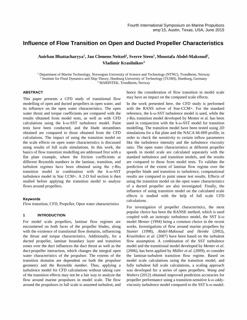
the model test results and empirical base lines. Fig. 1 shows

the results of the shear force coefficient (Cf) using the k-ω-

SST model and the γ-Reθ transition model in comparison to

the theoretical Blasius and Prandtl-von Karman lines. In

Fig. 1, ‘Transition’ and ‘Turbulent’ mean that γ-Reθ

transition model or the k-ω-SST model are applied,

respectively. The transition and turbulent CFD calculations

compare well to the theoretical curves.

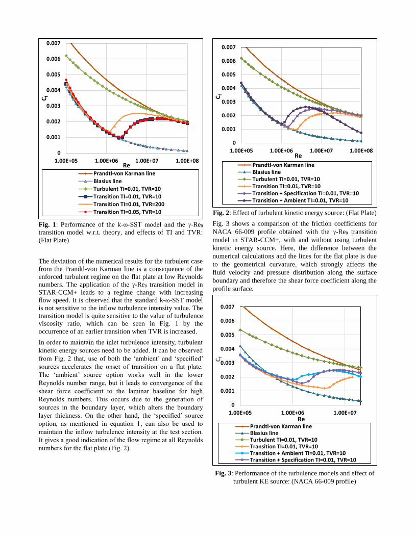
Fig. 1: Performance of the k-ω-SST model and the γ-Reθ

transition model w.r.t. theory, and effects of TI and TVR:

(Flat Plate)

The deviation of the numerical results for the turbulent case

from the Prandtl-von Karman line is a consequence of the

enforced turbulent regime on the flat plate at low Reynolds

numbers. The application of the γ-Reθ transition model in

STAR-CCM+ leads to a regime change with increasing

flow speed. It is observed that the standard k-ω-SST model

is not sensitive to the inflow turbulence intensity value. The

transition model is quite sensitive to the value of turbulence

viscosity ratio, which can be seen in Fig. 1 by the

occurrence of an earlier transition when TVR is increased.

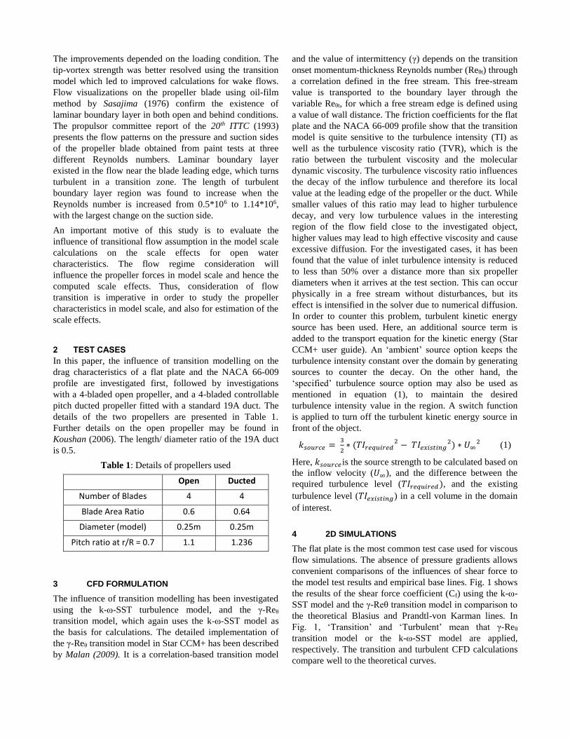
In order to maintain the inlet turbulence intensity, turbulent

kinetic energy sources need to be added. It can be observed

from Fig. 2 that, use of both the ‘ambient’ and ‘specified’

sources accelerates the onset of transition on a flat plate.

The ‘ambient’ source option works well in the lower

Reynolds number range, but it leads to convergence of the

shear force coefficient to the laminar baseline for high

Reynolds numbers. This occurs due to the generation of

sources in the boundary layer, which alters the boundary

layer thickness. On the other hand, the ‘specified’ source

option, as mentioned in equation 1, can also be used to

maintain the inflow turbulence intensity at the test section.

It gives a good indication of the flow regime at all Reynolds

numbers for the flat plate (Fig. 2).

Fig. 2: Effect of turbulent kinetic energy source: (Flat Plate)

Fig. 3 shows a comparison of the friction coefficients for

NACA 66-009 profile obtained with the γ-Reθ transition

model in STAR-CCM+, with and without using turbulent

kinetic energy source. Here, the difference between the

numerical calculations and the lines for the flat plate is due

to the geometrical curvature, which strongly affects the

fluid velocity and pressure distribution along the surface

boundary and therefore the shear force coefficient along the

profile surface.

Fig. 3: Performance of the turbulence models and effect of

turbulent KE source: (NACA 66-009 profile)

0

0.001

0.002

0.003

0.004

0.005

0.006

0.007

1.00E+05 1.00E+06 1.00E+07 1.00E+08

Cf

RePrandtl-von Karman line

Blasius line

Turbulent TI=0.01, TVR=10

Transition TI=0.01, TVR=10



0

0.001

0.002

0.003

0.004

0.005

0.006

0.007

1.00E+05 1.00E+06 1.00E+07 1.00E+08

Cf

Re

Prandtl-von Karman lineBlasius lineTurbulent TI=0.01, TVR=10Transition TI=0.01, TVR=10Transition + Specification TI=0.01, TVR=10Transition + Ambient TI=0.01, TVR=10

0

0.001

0.002

0.003

0.004

0.005

0.006

0.007

1.00E+05 1.00E+06 1.00E+07

Cf

RePrandtl-von Karman lineBlasius lineTurbulent TI=0.01, TVR=10Transition TI=0.01, TVR=10Transition + Ambient TI=0.01, TVR=10Transition + Specification TI=0.01, TVR=10

For the foil with two-dimensional flow effects, the

‘ambient’ specification works better than for the flat plate,

and gives comparatively closer shear force coefficient

values to the ‘specified’ source case. Thus the ‘specified’

source option is definitely a better choice for application to

transition study of model scale propellers, considering the

applicability to both the 2D cases at a wide range of

Reynolds numbers.

5 TRANSITION STUDY ON PROPELLERS

For the propeller simulations, the propeller and duct (in the

ducted propeller case) are defined by their respective

geometries which are used to generate local grids in STAR-

CCM+. The Multi Reference Frame (MRF) method is used,

where the propeller is fixed while its rotation is taken into

account by a local reference frame rotating at the desired

speed. The additional acceleration terms from the rotating

frame are incorporated into the modified equations of

motions. In the normal range of propeller operation the

interactions between moving and stationary parts can be

approximated with sufficient accuracy by the quasi-steady

solution, where the MRF approach is quite suitable. The

entire domain corresponds to one blade passage with

periodic boundary conditions. Fine wall normal mesh

required for the application of transition model (y+ <1), and

this has been achieved by using prismatic cells in the

boundary layer on the propeller blade and duct. Polyhedral

cells constitute the rest of the domain. The propeller model

with the mesh and domain is shown in Fig. 4.

Fig. 4: Open propeller model and domain in Star CCM+

For using the transition model, an inflow turbulence

intensity of 5% has been used, where good comparisons of

open water characteristics and flow patterns have been

obtained compared to model tests. This is similar to

observations made by Müller et al. (2009). To counter the

decay of the inflow turbulence, turbulence kinetic energy

sources are specified as mentioned in equation 1, the

sources being generated from the inlet to a distance of

0.6DP ahead of the propeller (Fig. 5). The full scale

simulations are performed using the k-ω-SST model, where

the propeller has a diameter of 20 times the model propeller.

For consistent comparison, topologically similar meshes

were used for both model and full scale simulations using

the low Reynolds near wall modelling.

Fig. 5: Specified TKE source distribution in Star CCM+

5.1 Open Water Characteristics

The open water thrust and torque coefficients, and open

water efficiency calculated using the transition model for

the open propeller have been compared to the calculations

using the k-ω-SST model, and results from model test

experiments. The comparisons at 5rps and 9rps propeller

speeds are presented in Table 2 and Table 3 respectively.

Table 2: Open water characteristics (open propeller: 5rps)

J

k-ω-SST

model

γ-Reθ

model

Model

test

KTP

0.3 0.477 0.478 0.470

0.5 0.371 0.375 0.375

0.7 0.267 0.273 0.266

10KQ

0.3 0.778 0.774 0.751

0.5 0.642 0.642 0.635

0.7 0.507 0.510 0.507

ηO

0.3 0.292 0.295 0.299

0.5 0.460 0.465 0.470

0.7 0.588 0.596 0.608

The transition model gives higher values of both propeller

thrust coefficient (KT) and torque coefficient (KQ) compared

to the k-ω-SST model at almost all propeller loadings for

both the tested speeds. This can be attributed to an

increment in the pressure component and a minute decrease

of the friction component of the blade forces when the

transition model is used compared to fully turbulent flow

assumptions. The resulting open water efficiency (ηO) is

closer to the value obtained from the model open water

tests. It has been further observed that, the open water

efficiency calculated from the model tests as well as the two

CFD calculations show consistent increments for the higher

propeller speed.

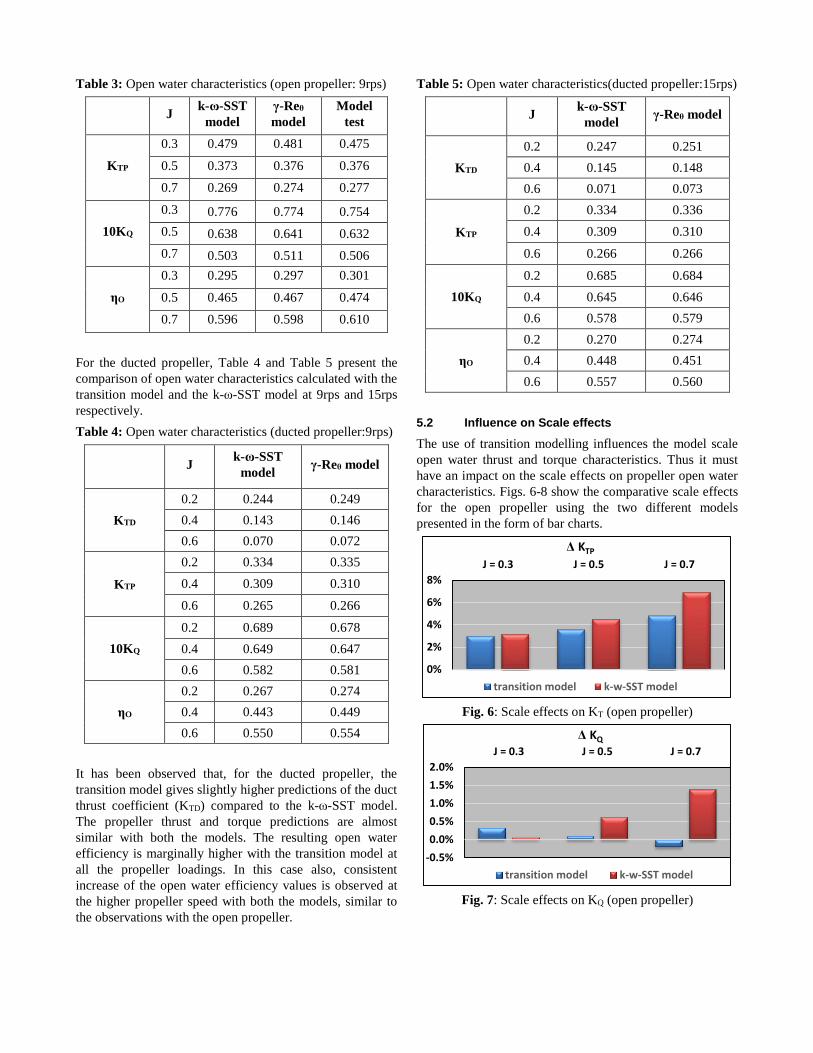
Table 3: Open water characteristics (open propeller: 9rps)

J k-ω-SST

model

γ-Reθ

model

Model

test

KTP

0.3 0.479 0.481 0.475

0.5 0.373 0.376 0.376

0.7 0.269 0.274 0.277

10KQ

0.3 0.776 0.774 0.754

0.5 0.638 0.641 0.632

0.7 0.503 0.511 0.506

ηO

0.3 0.295 0.297 0.301

0.5 0.465 0.467 0.474

0.7 0.596 0.598 0.610

For the ducted propeller, Table 4 and Table 5 present the

comparison of open water characteristics calculated with the

transition model and the k-ω-SST model at 9rps and 15rps

respectively.

Table 4: Open water characteristics (ducted propeller:9rps)

J

k-ω-SST

model γ-Reθ model

KTD

0.2 0.244 0.249

0.4 0.143 0.146

0.6 0.070 0.072

KTP

0.2 0.334 0.335

0.4 0.309 0.310

0.6 0.265 0.266

10KQ

0.2 0.689 0.678

0.4 0.649 0.647

0.6 0.582 0.581

ηO

0.2 0.267 0.274

0.4 0.443 0.449

0.6 0.550 0.554

It has been observed that, for the ducted propeller, the

transition model gives slightly higher predictions of the duct

thrust coefficient (KTD) compared to the k-ω-SST model.

The propeller thrust and torque predictions are almost

similar with both the models. The resulting open water

efficiency is marginally higher with the transition model at

all the propeller loadings. In this case also, consistent

increase of the open water efficiency values is observed at

the higher propeller speed with both the models, similar to

the observations with the open propeller.

Table 5: Open water characteristics(ducted propeller:15rps)

J

k-ω-SST

model γ-Reθ model

KTD

0.2 0.247 0.251

0.4 0.145 0.148

0.6 0.071 0.073

KTP

0.2 0.334 0.336

0.4 0.309 0.310

0.6 0.266 0.266

10KQ

0.2 0.685 0.684

0.4 0.645 0.646

0.6 0.578 0.579

ηO

0.2 0.270 0.274

0.4 0.448 0.451

0.6 0.557 0.560

5.2 Influence on Scale effects

The use of transition modelling influences the model scale

open water thrust and torque characteristics. Thus it must

have an impact on the scale effects on propeller open water

characteristics. Figs. 6-8 show the comparative scale effects

for the open propeller using the two different models

presented in the form of bar charts.

Fig. 6: Scale effects on KT (open propeller)

Fig. 7: Scale effects on KQ (open propeller)

0%

2%

4%

6%

8%

J = 0.3 J = 0.5 J = 0.7

Δ KTP

transition model k-w-SST model

-0.5%

0.0%

0.5%

1.0%

1.5%

2.0%

J = 0.3 J = 0.5 J = 0.7

Δ KQ


The scale effects are presented as the relative differences,

=(FS-MS)/MS*100%, between the full scale (FS) and

model scale (MS) values obtained at 9rps.

Fig. 8: Scale effects on ηO (open propeller)

For almost all the investigated cases, the propeller thrust

and torque are higher in the full scale for the open propeller,

the scale effects being more prominent for the thrust. As the

transition model gives higher propeller forces in the model

scale, the scale effects in general are reduced when these

values are compared to full scale propeller thrust and

torque. The scale effects on open water efficiency increase

with the advance ratio (J), which has been predicted by both

the models. The values obtained with the transition model

are lower in comparison to the k-ω-SST model, the

differences being close to 0.5% at all the loading conditions.

For this particular propeller, the calculated scale effects for

propeller torque are very small, and the values obtained

using the transition model are quite negligible, and smaller

in comparison to the results of k-ω-SST model.

Fig. 9: Scale effects on KTD (ducted propeller)

Fig. 10: Scale effects on KTP (ducted propeller)

Fig. 11: Scale effects on KQ (ducted propeller)

For the ducted propeller, Figs. 9-11 present the scale effect

comparisons for open water characteristics with the two

models. The full scale duct thrust coefficients are higher

than model scale values, while the propeller thrust and

torque coefficients are lower in full scale. The transition

model gives higher duct thrust in model scale (Fig. 9), and

hence causes a reduction in the calculated scale effects

compared to fully turbulent full scale calculations. Contrary

to the open propeller, the propeller thrust coefficient for the

ducted propeller decreases in full scale (Fig. 10) at all

advance coefficients, and the scale effects are slightly

higher with the transition model, though the magnitude is

less than 1.5% in all the cases. The propeller torque

coefficient decreases in full scale for the ducted propeller

(Fig. 11), and the scale effects are larger compared to those

observed for the open propellers (Fig. 7) under similar

loading conditions. These variations with scale are in

agreement with the results presented in earlier referred

works by Abdel-Maksoud and Heinke (2002) and

Krasilnikov et al (2007). Both the models give very similar

predictions of the scale effect on propeller torque, evident

from the similar predictions in model scale in Table 5.

6 PAINT TESTS

Paint tests were performed for the open propeller in the

towing tank at MARINTEK, Norway. The streamline

pattern over the propeller blade has been visualized at three

different propeller speeds corresponding to three values of

blade Reynolds numbers. The selected speeds cover very

well the transitional flow regime and the onset of turbulence

over the blade. The streamlines over the suction and

pressure sides at 5rps, 9rps, and 15rps are shown for the

design loading condition (J=0.7).

The paint streaks over the propeller blade give an indication

of the relative strength of the radial centrifugal force and the

tangential friction force. The lower friction force in the

laminar boundary layer allows the centrifugal force to

dominate, and results in radial paint streaks. On the

contrary, high friction in the turbulent boundary layer

causes the paint particles to follow a tangential path. The

transition zone can be recognized by a change in the paint

flow direction over the blade surface.

0%

2%

4%

6%

J = 0.3 J = 0.5 J = 0.7

Δ ηO


0%

4%

8%

12%

16%

J = 0.2 J = 0.4 J = 0.6

Δ KTD


-2.0%

-1.5%

-1.0%

-0.5%

0.0%

J = 0.2 J = 0.4 J = 0.6

Δ KTP


-5%

-4%

-3%

-2%

-1%

0%

J = 0.2 J = 0.4 J = 0.6

Δ KQ


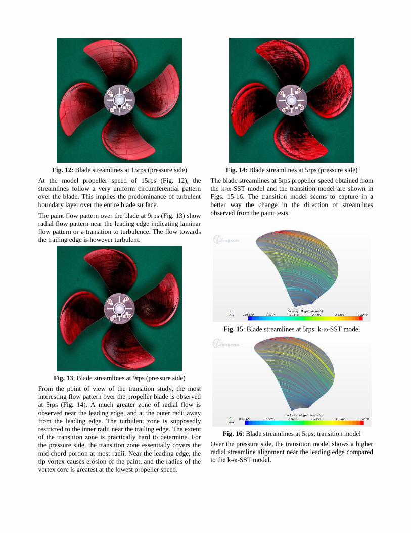
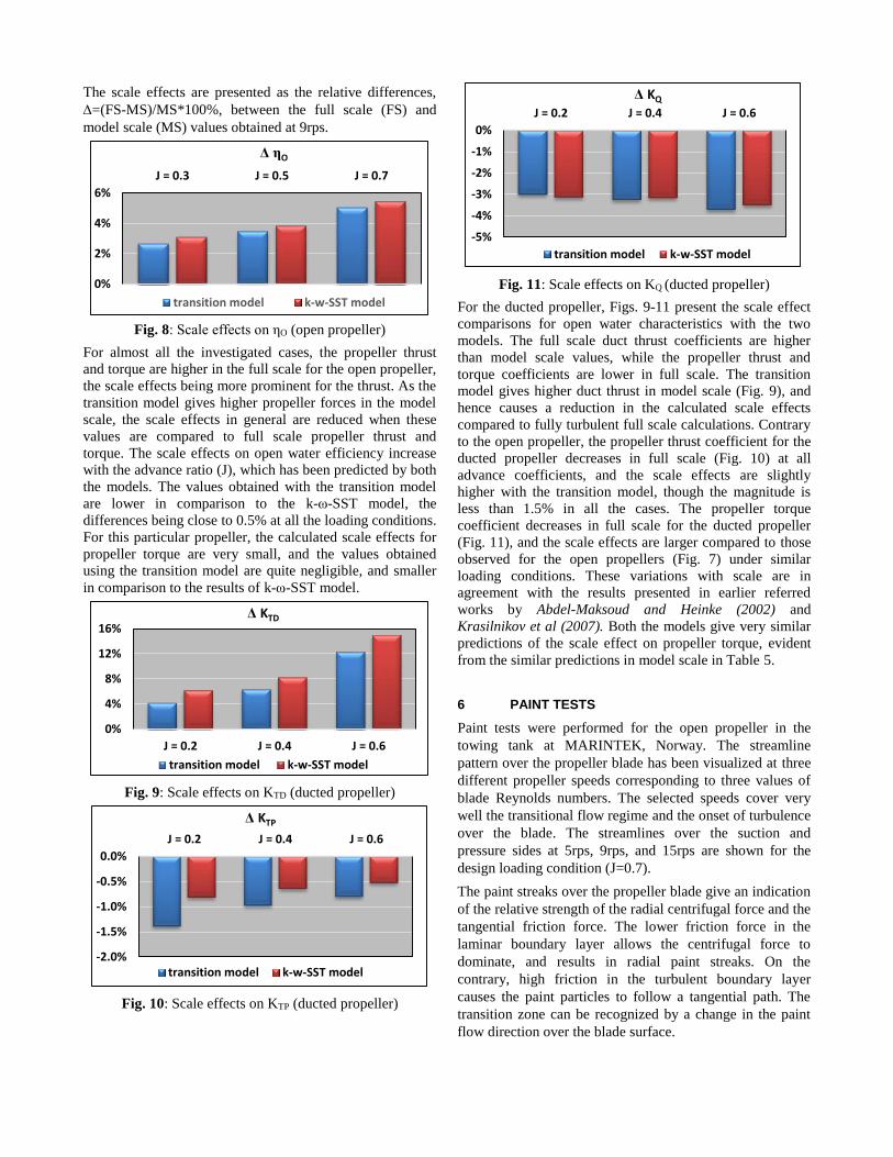
Fig. 12: Blade streamlines at 15rps (pressure side)

At the model propeller speed of 15rps (Fig. 12), the

streamlines follow a very uniform circumferential pattern

over the blade. This implies the predominance of turbulent

boundary layer over the entire blade surface.

The paint flow pattern over the blade at 9rps (Fig. 13) show

radial flow pattern near the leading edge indicating laminar

flow pattern or a transition to turbulence. The flow towards

the trailing edge is however turbulent.


From the point of view of the transition study, the most

interesting flow pattern over the propeller blade is observed

at 5rps (Fig. 14). A much greater zone of radial flow is

observed near the leading edge, and at the outer radii away

from the leading edge. The turbulent zone is supposedly

restricted to the inner radii near the trailing edge. The extent

of the transition zone is practically hard to determine. For

the pressure side, the transition zone essentially covers the

mid-chord portion at most radii. Near the leading edge, the

tip vortex causes erosion of the paint, and the radius of the

vortex core is greatest at the lowest propeller speed.


The blade streamlines at 5rps propeller speed obtained from

the k-ω-SST model and the transition model are shown in

Figs. 15-16. The transition model seems to capture in a

better way the change in the direction of streamlines

observed from the paint tests.

Fig. 15: Blade streamlines at 5rps: k-ω-SST model

Fig. 16: Blade streamlines at 5rps: transition model

Over the pressure side, the transition model shows a higher

radial streamline alignment near the leading edge compared

to the k-ω-SST model.

7 CONCLUSIONS

The influence of transition modelling on the flow around

marine propellers has been investigated, with respect to

propeller forces as well as the flow patterns over the blade

surface in model scale. The impact of using the γ-Reθ

transition model on the scale effects on open water

characteristics is discussed with the help of model and full

scale CFD calculations with the k-ω-SST model.

The flat plate simulations with the γ-Reθ transition model

implemented in Star CCM+ capture the onset of transition,

and provide good agreement of the friction coefficients at

different Reynolds numbers compared to the theoretical

Blasius and Prandtl-von Karman lines. This, along with the

simulations with the NACA 66-009 profile helped in tuning

different parameters and formed the basis for application of

the transition model for the complex flow around marine

propellers. Unlike the standard turbulence models, the

transition model is quite sensitive to inflow turbulence

parameters.

For the open propeller, the propeller thrust and torque

predictions with the transition model are higher compared

to the k-ω-SST model, mainly due to a higher pressure

component. The resulting open water efficiency predictions

are marginally better compared to model test calculations.

The propeller thrust and torque for the open propeller show

positive scale effects, due to higher full scale values

compared to model scale. The use of the transition

modelling in model scale has thus resulted in a reduction of

the scale effects. For the ducted propeller, the transition

model gives higher predictions of the duct thrust in the

model scale, and hence results in a corresponding lower

scale effect, as duct thrust is found to increase in full scale

for all propeller loadings. The propeller thrust and torque

for the ducted propeller decreases in full scale, the scale

effects being more for the torque. For the computed case,

the transition model gives very similar values of propeller

thrust and torque compared to the k-ω-SST model, and

hence the difference in the corresponding scale effects have

been very small.

The streamlines over the blade of the open propeller show

predominance of turbulent boundary layer over the entire

blade at the higher propeller speed of 15rps. The existence

of transition domains becomes visible at the lower speeds.

At the lowest propeller speed, a better prediction of the

streamline pattern is obtained with the transition model,

compared to the paint test results.

The use of transition modelling has a definite influence over

the flow patterns and the pressure and friction components

of the propeller forces in model scale, especially at lower

Reynolds numbers. However, for the cases investigated,

deviation of the propeller characteristics from the results of

the k-ω-SST model are not large, and further investigations

have to be carried out to apply the results of transition

modelling into a systematic scaling procedure for propeller

characteristics.

ACKNOWLEDGEMENT

The work presented here has been conducted within the

frameworks of the ongoing Competence building Project

PROPSCALE coordinated by MARINTEK (Norway) with

support from the Research Council of Norway (grant

number 225326). The consortium members include:

MARINTEK (Norway), Norwegian University of Science

and Technology (Norway), Aalesund University College

(Norway), Hamburg University of Technology (Germany),

China Ship Scientific Research Center (China), Havyard

Group AS (Norway), Rolls-Royce Marine AS (Norway),

Scana Volda AS (Norway) and VARD Design (Norway),

CD-Adapco.

NOMENCLATURE

n [Hz] Propeller rotational speed

D [m] Propeller diameter

V [m/s] Advance speed in open water

J [-] Advance coefficient (𝑉 𝑛𝐷⁄ )

TD [N] Duct thrust

TP [N] Propeller thrust

T [N] Total thrust

Q [N-m] Propeller Torque

KTP [-] Propeller thrust coefficient (𝑇𝑃 𝜌𝑛2𝐷4⁄ )

KTD [-] Duct thrust coefficient (𝑇𝐷 𝜌𝑛2𝐷4⁄ )

KQ [-] Torque coefficient (𝑄 𝜌𝑛2𝐷5⁄ )

ηO [-] Open water efficiency ( 𝐽𝐾𝑇 2𝜋𝐾𝑄⁄ )

REFERENCES

[1] Abdel-Maksoud, M. and Heinke, H.J. (2002),

“Scale Effects on Ducted Propellers,” Proceedings of 24th

Symposium on Naval Hydrodynamics, Fukuoka, Japan

[2] ITTC, 1993, “Report of the Propulsor Committee,”

Proceedings of the 20th ITTC, San Francisco, California

[3] Koushan, K. (2006), “Dynamics of ventilated

propeller blade loading on thrusters” Proceedings of

WMTC2006 World Maritime Technology Conference,

London

[4] Krasilnikov, V.I., Sun, J., Zhang, Zh., & Hong, F.

(2007), “Mesh generation technique for the analysis of

ducted propellers using a commercial RANSE solver and its

application to scale effect study,” Proceedings of the 10th

Numerical Towing Tank Symposium, (NuTTS’07),

Hamburg, Germany

[5] Malan, P. (2009) “Calibrating the γ-Reθ Transition

Model for Commercial CFD,” 47th AIAA Aerospace

Sciences Meeting

[6] Menter, F. R. (1994), “Two-Equation Eddy-

Viscosity Turbulence Models for Engineering

Applications,” AIAA Journal, Vol. 32, No. 8, pp. 1598-

1605.

[7 Müller, S-B., Abdel-Maksoud, M., Hilbert, G.

(2009), “Scale effects on propellers for large container

vessels,” Proceedings of the 1st International Symposium on

Marine Propulsors, (SMP’09), Trondheim, Norway

[8] Menter, F. R., Langtry, R. B., Likki, S. R., Suzen,

Y. B., Huang, P. G., and Volker, S. (2006), “A Correlation-

Based Transition Model Using Local Variables-Part I:

Model Formulation,” ASME J. Turbomach., 128, pp. 413–

422.

[9] Sasajima T. (1975) “A study on the Propeller

Surface Flow in Open and Behind Conditions”, 14th ITTC,

Contribution to Performance Committee, 1975

[10] User Guide: Star CCM+ 9.04.011, CD Adapco

[11] Wang, X. and Walters, K. (2012), “Computational

Analysis of Marine-Propeller Performance Using Transition

Sensitive Turbulence Modeling” ASME J. Fluids

Engineering, Vol-134

DISCUSSIONS

Question from Joao Baltazar

In the paper and in the presentation there is no information

on the iterative convergence of the RANS computations.

What are the maximum residuals when using the transition

model? In the presentation it was mentioned that γ=0 at L.E.

and γ=1 near the tip and/ or T.E. So, that means 0< γ<1 on

the blade surface. What can we say about transition in this

case? Seems that no transition to turbulence has occurred.

Authors’ reply

Thank you for your question. The convergence of blade and

duct coefficients as well as residuals are very satisfactory

when the γ-Reθ transition model is used, though the levels

of residuals are slightly higher compared to those obtained

with fully turbulent calculations. Fig. I shows the typical

residual convergence patterns obtained with the transition

model.

The domain of laminar and transition flow over the blade

surface is very much dependent on the propeller speed

(governing the blade Reynolds number), as well as the

loading condition. The distribution of intermittency (γ) over

an envelope around the blade and duct for J=0.6 at a

propeller speed of 9rps is shown in Fig. II.

Fig. I: Residuals with γ-Reθ transition model

Fig. II: Intermittency (γ) around propeller blade and duct

Comment from Jan Clemens Neitzel (co-author)

Using the ambient specification, the TKE sources lead to a

reduction of the boundary layer height with increasing

Reynolds numbers. The boundary layer height decreased to

a value comparable to the laminar flow estimation results.

Question from Antoine Ducoin

Where is the transition located along the blade span, and

how does it influence the overall characteristics?

Authors’ reply

Thank you for your question. The location and extent of

transition domain over the blade span depends on the

propeller speed and loading. The influence of using

transition model on propeller characteristics is shown in

Tables 2-5. The influence decreases with the increase of

propeller speed, as the blade streamline patterns become

turbulent (Figs. 12-14).

influence of flow transition on open and ducted propeller ... · influence of flow transition on...

Documents