inflation/unemployment regimes and the instability of … inflation/unemployment regimes and the...

1

Inflation/Unemployment Regimes and the Instability of the Phillips Curve

Paul Ormerod1

Bridget Rosewell2

Peter Phelps3

September 2009

1. Corresponding author Volterra Consulting, London, UK, [email protected] 2. Volterra Consulting, London, UK, [email protected] 3. Volterra Consulting and University of Cambridge, UK, [email protected]

JEL classification: C19, E31, N10 Keywords: Phillips curve, inflation, structural change, fuzzy clustering

mailto:[email protected]



2

Abstract

Using the statistical technique of fuzzy clustering, regimes of inflation and unemployment are explored for the

United States, the United Kingdom and Germany between 1871 and 2009. We identify for each country three

distinct regimes in inflation/unemployment space. There is considerable similarity across the countries in both

the regimes themselves and in the timings of the transitions between regimes. However, the typical rates of

inflation and unemployment experienced in the regimes are substantially different. Further, even within a

given regime, the results of the clusterings show persistent fluctuations in the degree of attachment to that

regime of inflation/unemployment observations over time. The economic implications of the results are that,

first, the inflation/unemployment relationship experiences from time to time major shifts. Second, that it is

also inherently unstable even in the short run. It is likely that the factors which govern the

inflation/unemployment trade off are so multi‐dimensional that it is hard to see that there is a way of

identifying periods of short run Phillips curves which can be assigned to particular historical periods with any

degree of accuracy or predictability. The short run may be so short as to be meaningless. The analysis shows

that reliance on any kind of trade off between inflation and unemployment for policy purposes is entirely

misplaced.

1. Introduction From a theoretical standpoint, Friedman (1968) argued that in the long‐run there is no connection

between inflation and the state of demand. In so far as there is consensus on these matters amongst

economists, this is it. However, the ‘long run’ is a theoretical concept, and economic theory offers no

guidance as to how long the long run might be in practice (though see Atkinson (1969) for a

fascinating analysis).

At any point in time, however, it is usually postulated that there is a connection between the rate of

inflation and the level of demand in the economy. The stronger is demand, the higher the rate of

inflation is likely to be. Yet discovering such a relationship in practice has proved fraught with

difficulties.

For example, there is no consensus as to the variable or variables which should be used empirically to

express the level of demand. Unemployment is frequently used, and was indeed chosen for the

seminal article on the Phillips curve attempting to describe the relationship between inflation and the

3

level of demand in pre‐First World War Britain (Phillips, 1958). But even then, different researchers

may estimate different functional forms for any particular empirical relationship.

Much more importantly, such relationships are well known not to be time invariant. In other words, a

reasonable relationship may be discovered to hold in a given economy over some particular period.

However, at some (unknown) point in the future, it will break down. This paper investigates whether

it is possible to identify points of breakdown and whether it makes sense to talk about a distinction

between short run and long run behaviour of the economy in this context.

The flattening of the Phillips curve in recent decades has been acknowledged globally. The

International Monetary Fund (IMF) reports that in many countries across the world, inflation is less

sensitive to business cycles in the 1990s than before (IMF, 2006). Various aspects of the instability in

the relationship between inflation and output have been highlighted in the postwar era. In the case

of the US, Atkeson and Ohanian (2001) show that between 1970 and 1999, there is no meaningful

relationship between inflation and unemployment. In another study, Roberts (2006) reports a near

halving of the slope of the US Phillips curve between 1960‐1983 and 1984‐2002. Furthermore, King,

Stock and Watson (1995) find that only upon introducing time‐variance into the model does there

appear to be any clear negative relationship between inflation and unemployment in the US during

the post‐Second World War era. It has also been suggested that the same negative slope of the

Phillips curve has shifted over time (King and Watson, 1994). These findings indicate that instability

potentially lies in both the slope and level of the Phillips curve.

Stability assessments, including structural break and recursive estimation tests for the Phillips curve

in Germany and the euro area, indicate that substantial parameter instability is present in the early

1980s and also around the time of reunification (Barkbu et al., 2005). The authors find that the

Phillips curve is relatively more unstable in Germany, compared to the US. It is suggested that the re‐

unification in Germany increased the instability of inflation‐unemployment relationship in the euro

area in the early 1990s. The flattening of the Phillips curve over recent decades in the UK has also

been documented (Iakova, 2007).

4

Reasons for this instability that have been suggested are not always independent of each other, but

generally relate to some form of structural change in the economy. For example, greater labour

market competition may reduce the cyclical sensitivity of profit margins. Businesses are more limited

in their ability to raise their prices in response to increased demand (Batini, Jackson and Nickell,

2005).

It has also been suggested that production costs have become less sensitive to the business cycle. In

the case of developed western economies, there has been an increasing trend in businesses

transferring some of their activities to countries such as China and India. This has made workers less

inclined to push for higher wages as unemployment rates fall. Therefore the impact of economic

activity on marginal cost of labour may have changed in the modern era. The ability of firms to hire

workers from Accession countries of Eastern Europe and the increased flow of immigration from such

countries is also likely to have had similar effects (Bean, 2006).

The famous “Lucas Critique”, originating from a paper by Robert Lucas in 1976, is also relevant when

considering the instability of parameters in economic models. The “Lucas Critique” concerns the

behaviour of the policymaker influencing the economic agents’ behaviour. Consider a change in

monetary regime from an inflation‐targeting regime to an alternative one, where the central bank

attempts to permanently climb the Phillips curve (by trading off higher inflation for lower

unemployment). The change in behaviour of the central bank would, at some point, influence the

behaviour of economic agents. For example, firms would foresee higher inflation in the future and

make new decisions over employment levels. Thus the policy change would likely alter the estimated

parameters of the Phillips curve.

Although the empirical support for the “Lucas Critique” is rather mixed, researchers have pointed

towards monetary policy regime changes as having an impact on the Phillips curve. It is considered

that credible monetary policy has improved the ability of central banks to anchor inflation

expectations, thus dampening the impact of real economic activity on inflation and flattening the

Phillips curve (Mishkin, 2007).

5

There have been numerous country‐specific structural changes in the modern economy which have

potentially altered the relationship between inflation and real economic activity. In Germany, the re‐

unification and adoption of the Euro currency are two relatively recent structural changes to have

occurred. In the US, the Federal Reserve became more aggressive in the fight against high inflation

following the economic distress of the 1970s. In the UK, the independence of the Bank of England is

thought to have made monetary policy more credible.

All of these propositions are essentially post hoc justifications for changes in a relationship which has

its roots in an empirical association of economic aggregates. An important implication of the

literature on empirical Phillips curves is that there is no settled view as to how and why they break

down, with many reasons being put forward, both of a general and a country‐specific nature. But

break down they undoubtedly do.

In this paper, we characterise the inherent instability of the empirical Phillips curve using annual data

in three major economies, the United States, the United Kingdom and Germany over the period 1871

– 2009. There are two inherent reasons for the instability of empirical Phillips curves. First, these

major capitalist economies each operate at any point in time in one of three distinct regimes in

inflation/unemployment rate space. The probability of remaining at time (t+1) in the regime which

obtains at time t is high, but there is a probability of switching to a different regime. We obtain

empirical estimates of the transition probability matrices.

We use the statistical technique of fuzzy clustering to illustrate these points, using long run data for

Germany, the United Kingdom and the United States. This approach has the important attribute of

expressing the strength of association of any given observation with a particular regime rather than

creating a simple classification.

This brings us to the second reason for the instability of the Phillips curves. Not only do economies

move from one regime to another, but the observations within any given regime have different

degrees of membership of it. An observation is allocated to a particular regime because its

attributes, on which the clustering is carried out, have more in common with those observations in

6

this regime than in other regimes. However, the degree to which this is the case varies, from being

only marginally closer to one group than to another, to being unequivocally in one group to the

exclusion of others. The degrees of memberships of inflation/unemployment regimes constantly

fluctuate over time within any given regime.

The economic implications of the results described here are that there are occasional major

shocks/changes in economic behaviour which move economies from one inflation/unemployment

regime to another. And importantly, in addition, there is a continuous sequence of small shocks

which change the degree to which observations can be characterised as belonging to the same

regime.

Section 2 describes the data, section 3 the technique of fuzzy clustering, and section 4 sets out the

results.

2. Data

The main sources for the historical data are Maddison (1995) and Mitchell (1978). United States pre‐

Second World War unemployment data is taken from Romer (1986) and Coen (1973). Data since

1994 is available in the IMF database.

A striking feature of the data over the 1871‐2009 period is the similarity of the distributions in

inflation rates between the three countries, where inflation is defined as the percentage change in

the consumer price index. There is of course the quite exceptional period in Germany in the early

1920s, culminating in the hyperinflation of 1924. We exclude these years from the analysis. To

anticipate, we identify three regimes in inflation/unemployment space in each country, so strictly

speaking we identify four regimes, with the massive German inflation 1920‐24 constituting a separate

regime.

Table 1 sets out the summary statistics for inflation 1871‐2009 in the three countries (excluding 1920‐

1924 for Germany, a point we do not repeat below)

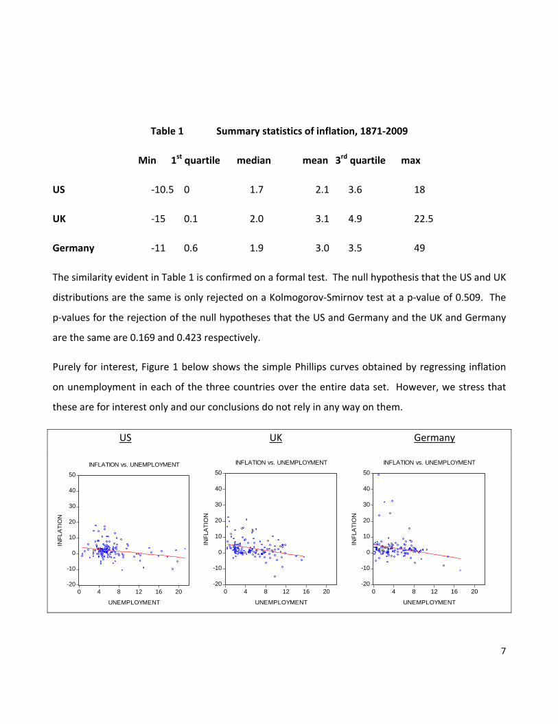
Table 1 Summary statistics of inflation, 1871‐2009

Min 1st quartile median mean 3rd quartile max

US ‐10.5 0 1.7 2.1 3.6 18

UK ‐15 0.1 2.0 3.1 4.9 22.5

Germany ‐11 0.6 1.9 3.0 3.5 49

The similarity evident in Table 1 is confirmed on a formal test. The null hypothesis that the US and UK

distributions are the same is only rejected on a Kolmogorov‐Smirnov test at a p‐value of 0.509. The

p‐values for the rejection of the null hypotheses that the US and Germany and the UK and Germany

are the same are 0.169 and 0.423 respectively.

Purely for interest, Figure 1 below shows the simple Phillips curves obtained by regressing inflation

on unemployment in each of the three countries over the entire data set. However, we stress that

these are for interest only and our conclusions do not rely in any way on them.

US UK Germany

-20

-10

0

10

20

30

40

50

0 4 8 12 16 20

UNEMPLOYMENT

INF

LAT

ION

INFLATION vs. UNEMPLOYMENT

-20

-10

0

10

20

30

40

50

0 4 8 12 16 20

UNEMPLOYMENT

INF

LAT

ION


-20

-10

0

10

20

30

40

50

0 4 8 12 16 20

UNEMPLOYMENT

INF

LAT

ION


7

8

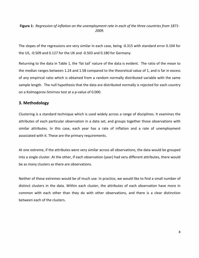
Figure 1: Regression of inflation on the unemployment rate in each of the three countries from 1871‐2009.

The slopes of the regressions are very similar in each case, being ‐0.315 with standard error 0.104 for

the US, ‐0.509 and 0.127 for the UK and ‐0.503 and 0.180 for Germany.

Returning to the data in Table 1, the ‘fat tail’ nature of the data is evident. The ratio of the mean to

the median ranges between 1.24 and 1.58 compared to the theoretical value of 1, and is far in excess

of any empirical ratio which is obtained from a random normally distributed variable with the same

sample length. The null hypothesis that the data are distributed normally is rejected for each country

on a Kolmogorov‐Smirnov test at a p‐value of 0.000.

3. Methodology

Clustering is a standard technique which is used widely across a range of disciplines. It examines the

attributes of each particular observation in a data set, and groups together those observations with

similar attributes. In this case, each year has a rate of inflation and a rate of unemployment

associated with it. These are the primary requirements.

At one extreme, if the attributes were very similar across all observations, the data would be grouped

into a single cluster. At the other, if each observation (year) had very different attributes, there would

be as many clusters as there are observations.

Neither of these extremes would be of much use. In practice, we would like to find a small number of

distinct clusters in the data. Within each cluster, the attributes of each observation have more in

common with each other than they do with other observations, and there is a clear distinction

between each of the clusters.

Classical clustering groups each observation, on the basis of its attributes, unequivocally into one or

other of the clusters. We overlay classical clustering techniques with fuzzy logic and use fuzzy

clustering.

Fuzzy clustering assigns each observation to some degree to each of the clusters. In the jargon, each

observation has a membership of each cluster. Membership is calculated as a proportion, so the sum

of the memberships of each observation is 1. An observation which is very typical of a particular

cluster will have a membership of that cluster of close to 1, and close to zero for the other clusters.

On the other hand, an observation which is a more marginal member will have a similar membership

value for two (or very occasionally more) clusters. It will be allocated to the cluster for which its

membership is highest, but it has attributes which place it on the margin between clusters.

Fuzzy clustering therefore contains more information in its output than classical clustering. The

concept of membership and how this might evolve in future is a key part of the calculations of the

potential range of inflation.

More specifically, we start with a data set X consisting of n observations, where each observation is a

vector in a d‐dimensional space. The aim of clustering is to divide the data into c clusters, where c can

be between 2 and n. The divisions should be such that within the clusters the data have similar

characteristics and the average difference between cluster characteristics is maximised.

The attributability of observation xj to cluster k is ukj . With classical clustering ukj can only take the

value 0 or 1, but with fuzzy clustering it can take any value between 0 and 1.

Classical clustering,

)1(}1,0{kju

Fuzzy clustering,

9

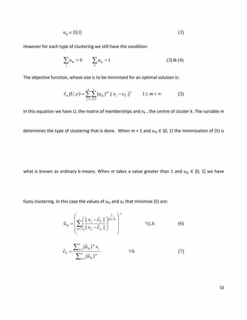
)2(]1,0[kju

However for each type of clustering we still have the condition:

)4(&)3(10 k

kjj

kj uu

The objective function, whose size is to be minimised for an optimal solution is:

)5(1||||)(),( 2

1 1

mxuUJ kj

n

j

c

k

mkjm

In this equation we have U, the matrix of memberships and vk , the centre of cluster k. The variable m

determines the type of clustering that is done. When m = 1 and ukj {0, 1} the minimisation of (5) is

what is known as ordinary k‐means. When m takes a value greater than 1 and ukj [0, 1] we have

fuzzy clustering. In this case the values of ukj and vk that minimise (5) are:

)6(,||ˆ||

||ˆ||u

1

1

)1(

2

kjx

xc

g

m

gj

kjkj

)7()ˆ(

)ˆ(ˆ

1

1 ku

xun

j

mkj

n

j jm

kj

k

10

As the centres of the clusters are not known before the clustering process, the memberships cannot

be calculated directly, and an iterative process has to be used. The optimal ukj can be found by

repeating the following process

(i) m and cluster number c are assumed, and a norm in equation (5) is defined appropriately (for

our purposes, the standard Euclidean norm). In addition, an initial value U(0) Mfc is set for U

(where Mfc is the space satisfying the above conditions (2), (3) and (4) ). The value can be

taken at random.

(ii) The cluster centre vk(0) is calculated using U(0) and equation (7)

(iii) U(1) is calculated using vk(0) and equation (6)

(iv) Defining an appropriate norm and threshold value , the preceding steps are repeated until

|||| )1()( pp UU

11

n (6).

When the inequality in step (iv) is satisfied, we are left with the c optimal cluster centres , vk(p),

whose memberships U(p) are given by equatio

There is no absolutely unequivocal way of determining the optimal number of clusters in any given

data set. However, a formal tool which is widely used to calculate this is the Dunn coefficient

(Kaufman and Rousseeuw, 1990). The coefficient is calculated with the data grouped into a single

cluster, into two clusters, and so on up to N clusters. The cluster number which maximises the value

of this coefficient is a reliable number of clusters to choose.

Dunn’s coefficient is a measure of how well n observations are classified into c clusters by a clustering

algorithm:

n

j

c

kkjn

D1 1

21

Where is a measure of the distance of observation j from the centre of cluster k, normalised so

that .

kj

1

kj 1

c

k

If an object is equidistant from all cluster centres ckj 1 kand the theoretical minimum value

of D (although it is difficult to see how this would happen in practice) is cc

ncn

D111

2min .

Therefore the range of D , 11 Dc , is dependent on c, so in order to compare the Dunn’s

coefficient of clusterings using different c, it is necessary to use the standardised Dunn’s coefficient:

c

DD

11c

1~

.

A certain amount of judgment may still be involved in the case where two or even three cluster

numbers have similar values for the coefficient, but the Dunn coefficient offers a helpful guide to the

number of clusters to choose.

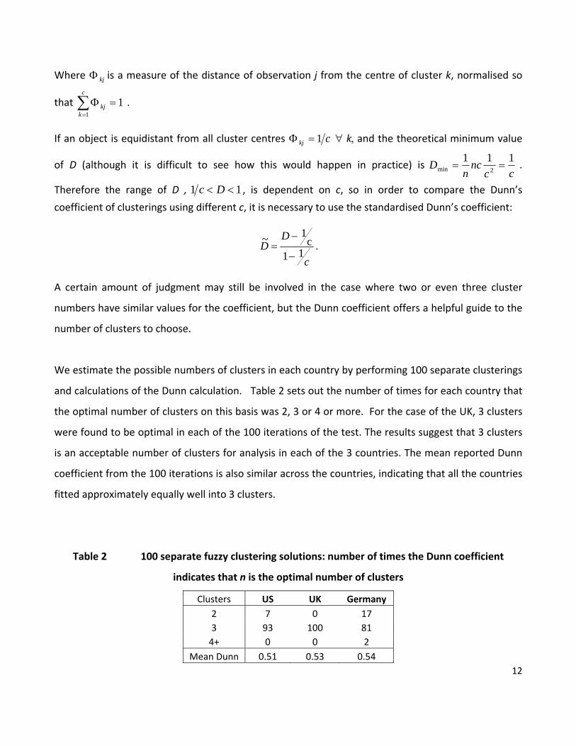
We estimate the possible numbers of clusters in each country by performing 100 separate clusterings

and calculations of the Dunn calculation. Table 2 sets out the number of times for each country that

the optimal number of clusters on this basis was 2, 3 or 4 or more. For the case of the UK, 3 clusters

were found to be optimal in each of the 100 iterations of the test. The results suggest that 3 clusters

is an acceptable number of clusters for analysis in each of the 3 countries. The mean reported Dunn

coefficient from the 100 iterations is also similar across the countries, indicating that all the countries

fitted approximately equally well into 3 clusters.

Table 2 100 separate fuzzy clustering solutions: number of times the Dunn coefficient

indicates that n is the optimal number of clusters

Clusters US UK Germany

2 7 0 17

3 93 100 81

4+ 0 0 2

Mean Dunn 0.51 0.53 0.54

12

13

4. Results

For each country, we carried out 500 separate calculations of the fuzzy clustering algorithm, and

report the averages across the 500 solutions. We first describe the values of inflation and

unemployment at the centre of each cluster. The fuzzy clustering algorithm, once the number of

clusters is decided, allocates each observation a degree of membership of each of the clusters. As

noted above, the degree for any particular cluster can be between 0 and 1 (or 0 and 100 per cent),

and the sum of the degrees across the clusters for any given observation is 1 (100 per cent). Each

observation is allocated to the cluster for which its degree of membership is highest. For the most

part, the degree to which it is in this cluster is high compared to its degrees of membership of the

other clusters, but there are some observations which lie on the borderline between two clusters.

The cluster centres are the values of the attributes, in this case inflation and unemployment, of a

hypothetical observation whose degree of membership of that cluster is 1.

We then go on to present information on the degrees of membership of the clusters for the

observations on a time series basis.

4.1 US Cluster Analysis

Averaged over 500 separate solutions of the fuzzy cluster algorithm, the values of inflation and

unemployment at the centre of each cluster can be calculated and are shown below in Table 3

Table 3 Values for US inflation and unemployment rates at cluster centres, averaged across

500 separate solutions of the fuzzy clustering algorithm

Cluster

Description Inflation Unemployment Observations

Steady 0.9 5.1 85

Weak ‐1.7 14.2 17

14

Disruption 6.7 5.8 37

The first cluster has low inflation and low unemployment. Of the 139 years in the data set, 85 are

allocated to this cluster. The majority of the last 15 years have fallen into this category. For purposes

of description, we call this cluster ‘steady’.

The second cluster is characterised by low inflation/deflation and high unemployment. This cluster is

the least common, and figures the most heavily around the time of the Great Depression. We have

labelled it ‘weak’.

The final cluster shows moderate to high inflation and moderate unemployment. More than one

quarter of the data belong to this cluster and it has been labelled ‘disruption’. Years with high

membership of the cluster are the war years and the years around the oil price hikes in the 1970s.

Figure 2 below draws on the fact that fuzzy clustering allocates any given observation a degree of

membership of each cluster, in contrast to classical clustering which allocates it unequivocally to one

or the other cluster. Figure 2 shows the degree of membership of each of the clusters for each

annual observation in the US 1871‐2009.

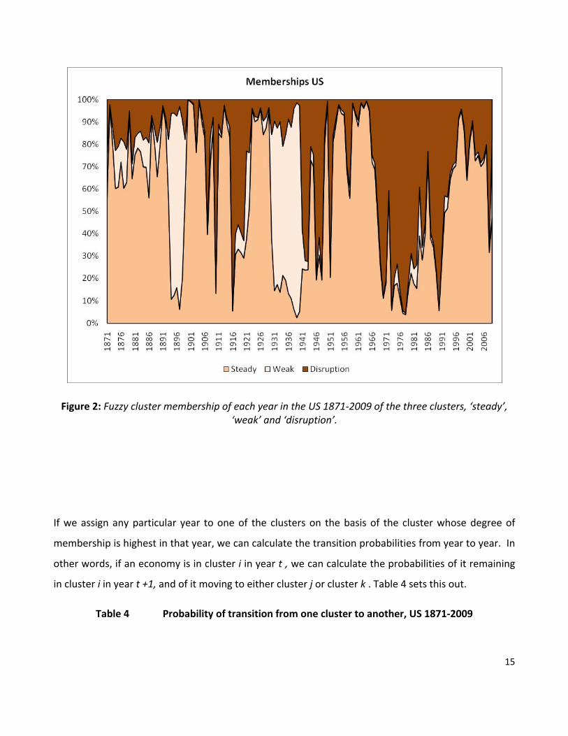
Figure 2: Fuzzy cluster membership of each year in the US 1871‐2009 of the three clusters, ‘steady’, ‘weak’ and ‘disruption’.

If we assign any particular year to one of the clusters on the basis of the cluster whose degree of

membership is highest in that year, we can calculate the transition probabilities from year to year. In

other words, if an economy is in cluster i in year t , we can calculate the probabilities of it remaining

in cluster i in year t +1, and of it moving to either cluster j or cluster k . Table 4 sets this out.

Table 4 Probability of transition from one cluster to another, US 1871‐2009

15

16

Transition Matrix

US T2

Cluster Steady Weak Disruption

Steady 0.87 0.02 0.11

Weak 0.12 0.82 0.06 T1

Disruption 0.24 0.03 0.73

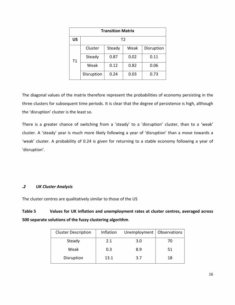
The diagonal values of the matrix therefore represent the probabilities of economy persisting in the

three clusters for subsequent time periods. It is clear that the degree of persistence is high, although

the ‘disruption’ cluster is the least so.

There is a greater chance of switching from a ‘steady’ to a ‘disruption’ cluster, than to a ‘weak’

cluster. A ‘steady’ year is much more likely following a year of ‘disruption’ than a move towards a

‘weak’ cluster. A probability of 0.24 is given for returning to a stable economy following a year of

‘disruption’.

.2 UK Cluster Analysis

The cluster centres are qualitatively similar to those of the US

Table 5 Values for UK inflation and unemployment rates at cluster centres, averaged across

500 separate solutions of the fuzzy clustering algorithm.

Cluster Description Inflation Unemployment Observations

Steady 2.1 3.0 70

Weak 0.3 8.9 51


The first is the ‘steady’ cluster with reasonably low levels of inflation and unemployment. The

majority of observations fall into this cluster. The second is the ‘weak’ cluster and has high

unemployment and low inflation. This is similar to the US ‘weak’ cluster, although in the UK this

accounts for more than a third of total memberships. The final cluster is characterised by high

inflation and moderate unemployment and is thus labelled ‘disruption’. This cluster is apparent

during the First and Second World Wars as well as the 1970s oil crisis.

Whereas most of the past 15 years have fallen into the ‘steady’ category, there has recently been a

noticeable shift towards the ‘weak’ cluster.

Figure 3: Fuzzy cluster membership of each year in the UK 1871‐2009 of the three clusters, ‘steady’, ‘weak’ and ‘disruption’.

17

18

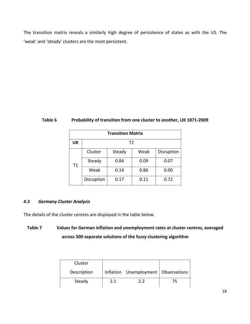
The transition matrix reveals a similarly high degree of persistence of states as with the US. The

‘weak’ and ‘steady’ clusters are the most persistent.

Table 6 Probability of transition from one cluster to another, UK 1871‐2009

Transition Matrix

UK T2

Cluster Steady Weak Disruption

Steady 0.84 0.09 0.07

Weak 0.14 0.86 0.00 T1


4.3 Germany Cluster Analysis

The details of the cluster centres are displayed in the table below.

Table 7 Values for German inflation and unemployment rates at cluster centres, averaged

across 500 separate solutions of the fuzzy clustering algorithm

Cluster

Description Inflation Unemployment Observations

Steady 2.1 2.2 75

19

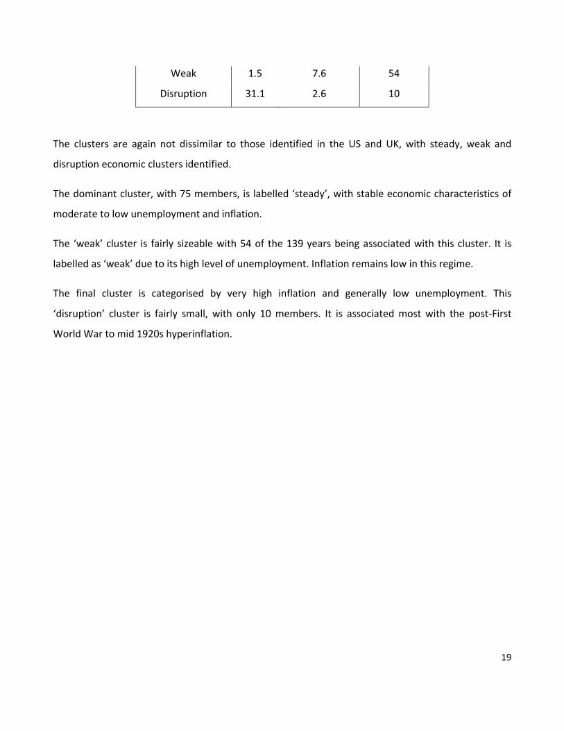
Weak 1.5 7.6 54


The clusters are again not dissimilar to those identified in the US and UK, with steady, weak and

disruption economic clusters identified.

The dominant cluster, with 75 members, is labelled ‘steady’, with stable economic characteristics of

moderate to low unemployment and inflation.

The ‘weak’ cluster is fairly sizeable with 54 of the 139 years being associated with this cluster. It is

labelled as ‘weak’ due to its high level of unemployment. Inflation remains low in this regime.

The final cluster is categorised by very high inflation and generally low unemployment. This

‘disruption’ cluster is fairly small, with only 10 members. It is associated most with the post‐First

World War to mid 1920s hyperinflation.

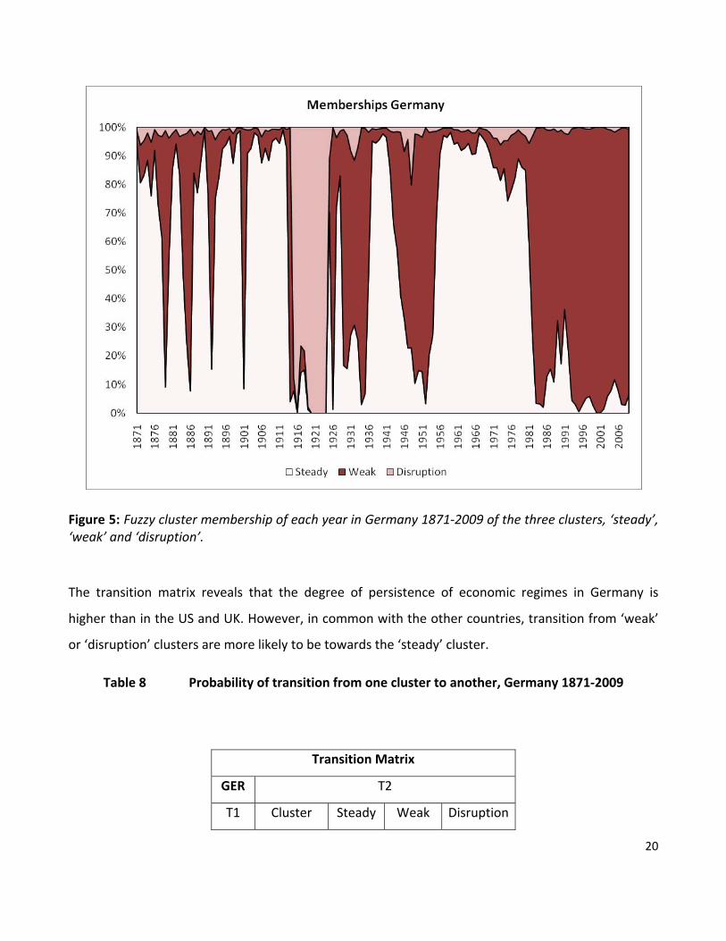
Figure 5: Fuzzy cluster membership of each year in Germany 1871‐2009 of the three clusters, ‘steady’, ‘weak’ and ‘disruption’.

The transition matrix reveals that the degree of persistence of economic regimes in Germany is

higher than in the US and UK. However, in common with the other countries, transition from ‘weak’

or ‘disruption’ clusters are more likely to be towards the ‘steady’ cluster.

Table 8 Probability of transition from one cluster to another, Germany 1871‐2009

Transition Matrix

GER T2

T1 Cluster Steady Weak Disruption

20

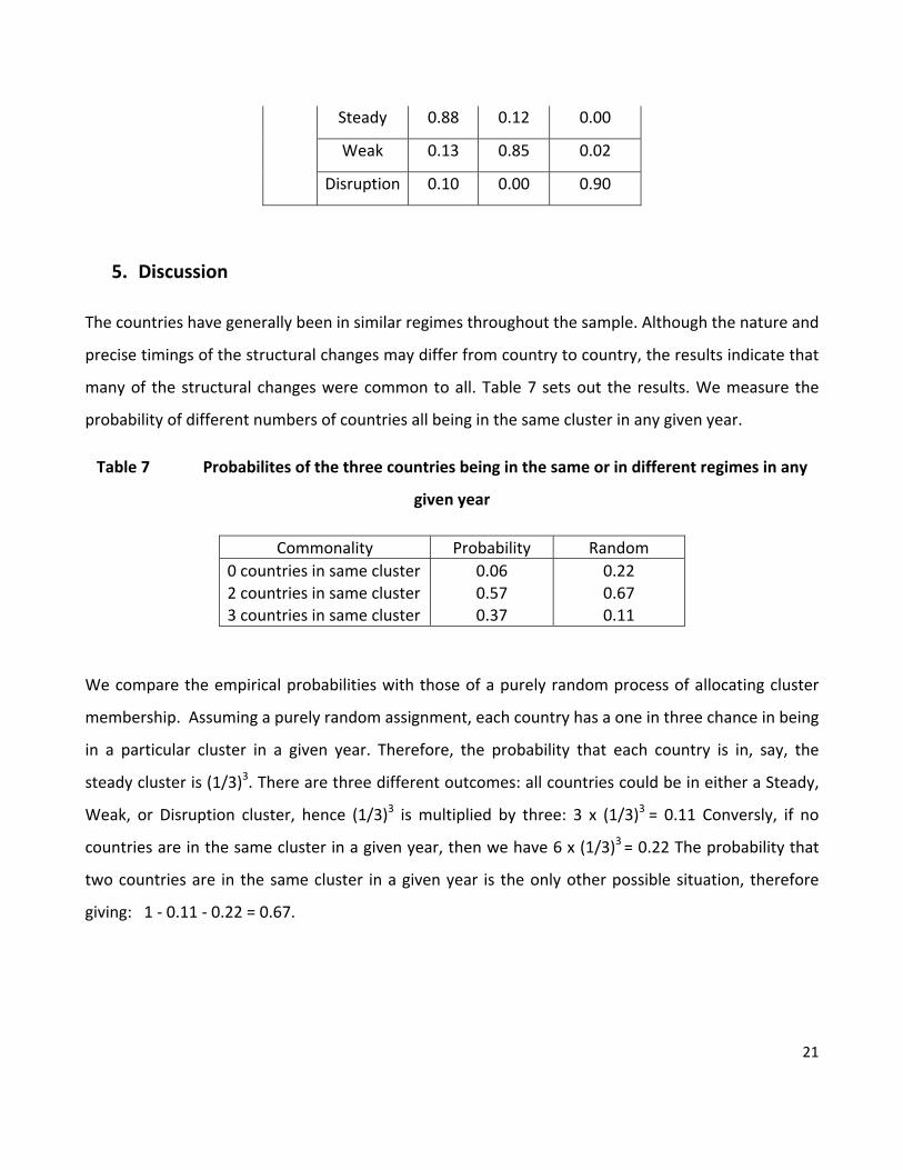
21

Steady 0.88 0.12 0.00

Weak 0.13 0.85 0.02


5. Discussion

The countries have generally been in similar regimes throughout the sample. Although the nature and

precise timings of the structural changes may differ from country to country, the results indicate that

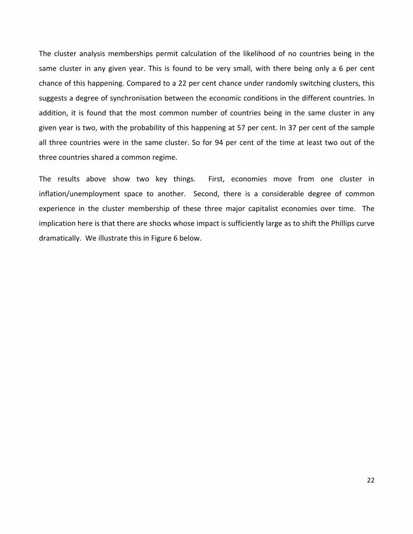
many of the structural changes were common to all. Table 7 sets out the results. We measure the

probability of different numbers of countries all being in the same cluster in any given year.

Table 7 Probabilites of the three countries being in the same or in different regimes in any

given year

Commonality Probability Random

0 countries in same cluster 0.06 0.22

2 countries in same cluster 0.57 0.67 3 countries in same cluster 0.37 0.11

We compare the empirical probabilities with those of a purely random process of allocating cluster

membership. Assuming a purely random assignment, each country has a one in three chance in being

in a particular cluster in a given year. Therefore, the probability that each country is in, say, the

steady cluster is (1/3)3. There are three different outcomes: all countries could be in either a Steady,

Weak, or Disruption cluster, hence (1/3)3 is multiplied by three: 3 x (1/3)3 = 0.11 Conversly, if no

countries are in the same cluster in a given year, then we have 6 x (1/3)3 = 0.22 The probability that

two countries are in the same cluster in a given year is the only other possible situation, therefore

giving: 1 ‐ 0.11 ‐ 0.22 = 0.67.

22

The cluster analysis memberships permit calculation of the likelihood of no countries being in the

same cluster in any given year. This is found to be very small, with there being only a 6 per cent

chance of this happening. Compared to a 22 per cent chance under randomly switching clusters, this

suggests a degree of synchronisation between the economic conditions in the different countries. In

addition, it is found that the most common number of countries being in the same cluster in any

given year is two, with the probability of this happening at 57 per cent. In 37 per cent of the sample

all three countries were in the same cluster. So for 94 per cent of the time at least two out of the

three countries shared a common regime.

The results above show two key things. First, economies move from one cluster in

inflation/unemployment space to another. Second, there is a considerable degree of common

experience in the cluster membership of these three major capitalist economies over time. The

implication here is that there are shocks whose impact is sufficiently large as to shift the Phillips curve

dramatically. We illustrate this in Figure 6 below.

1880 1900 1920 1940 1960 1980 2000

Date

0

1

0

1

0

1

weak by date

steady by date

disruption by date

Average Memberships 1871-2009

Mem

ber

ship

Figure 6: Average membership of ‘weak’, ‘steady’ and ‘disruption’ clusters, 1871‐2009.

It is apparent from Figure 6 that there are several commonalities. The First World War created much

‘disruption’ for all three economies, with substantial levels of inflation being recorded. The years

around the Great Depression show up as ‘weak’ in all countries, with unemployment levels very high

and substantial deflation experienced by all.

The period before the First World War shows little membership of the disruption regime but rapid

swings between membership of the ‘steady’ and ‘weak’ group. On average the 1960s show the most

consistently strong memberships.

A prolonged period of relative stability was experienced for around 20 years following the Second

World War. This stability persisted for longer in Germany, whilst both the US and UK suffered a

decade of disruption which was marked by stagflation.

23

24

Notably, it is difficult to identify significant periods with high memberships of one regime persisting.

Mixtures are prevalent as well changes in these mixtures.

The natural instinct of economists when confronted by evidence of a distinct shift in an important

empirical relationship is to to try to identify a major change which can account for this. Sometimes,

this will be successful. However, we note in this context that recent research in network theory,

describing the percolation of shocks across a system of interconnected agents, suggests that it is

possible for even minor shocks to have dramatic consequences (for example, Watts, 2002; Ormerod

and Colbaugh, 2006). An example is the massive stockmarket crash in October 1987, for which no

major cause has ever been identified.

A further implication of Figure 6, however, is that although transitions from one

inflation/unemployment regime to another are relatively rare, there are persistent fluctuations in the

degrees of membership of a regime, even in periods of relative stability in terms of the dominant

regime. These imply in turn that the instability of the short‐run empirical Phillips curve is endemic.

The factors which govern the inflation/unemployment trade off are so multi‐dimensional that it is not

really possible to identify them empirically. There may be periods when an estimated relationship

appears to exist, but of necessity it will break down even in the absence of any major shock which

might enable the breakdown to be identified.

In this context it is hard to see that there is a way of identifying periods of short run Phillips curves

which can be assigned to particular historical periods with any degree of accuracy or predictability.

The short run may be so short as to be meaningless and in addition the clustering shows how

unpredictable transitions to new regime memberships will be. If nothing else, this analysis shows

that reliance on any kind of trade off between inflation and unemployment for policy purposes is

entirely misplaced.

25

References

1. A.Atkeson and L. Ohanian, 2001, “Are Phillips Curves Useful for Forecasting Inflation?",

Federal Reserve Bank of Minneapolis Quarterly Review, 25(1), pp. 2‐11.

2. B. Barkbu, V. Cassino, A. Gosselin‐Lotz, L Piscitelli, 2005, “The New Keynesian Phillips Curve in

the United States and the Euro Area: Aggregation Bias, Stability and Robustness,” Bank of

England Working Paper No. 285.

3. N. Batini, B. Jackson, and S. Nickell, 2005, “An Open Economy New Keynesian Phillips Curve for

the UK”, Journal of Monetary Economics, 52, pp. 1061‐1071.

4. C. Bean, “Globalisation and Inflation”, Speech to LSE Economics Society, Oct. 2006.

5. R. Coen 1973, “Labor Force and Unemployment in the 1920s and 1930s: A Re‐examination

based on Postwar Experience”, The Review of Economics and Statistics, 55(1):46‐55.

6. M. Friedman, 1968, "The Role of Monetary Policy", AER, 58(1), pp. 1‐17.

7. D. Iakova, 2007, “Flattening of the Phillips Curve: Implications for Monetary Policy”, IMF

Working Paper 07/76.

8. International Monetary Fund, World Economic Outlook, IMF, April 2006.

9. L. Kaufman, and P. Rousseeuw, Finding Groups in Data: An Introduction to Cluster Analysis,

1990 Wiley, New York.

10. R. King and M. Watson, 1994, “The post‐war U.S. Phillips curve: A Revisionist Econometric

History”, Carnegie‐Rochester Conference Series on Public Policy, Vol. 41, pp. 157–219.

11. R. King, J. Stock, and M. Watson, 1995, “Temporal Instability of the Unemployment‐Inflation

Relationship”, Federal Reserve Bank of Chicago Economic Perspectives Vol. 19, pp. 2‐12.

12. R. Lucas, 1976, “Econometric Policy Evaluation: A Critique,” Carnegie‐Rochester Conference

Series on Public Policy, 1, pp. 19‐46.

13. A.Maddison, Dynamic Forces in Capitalist Development, Oxford University Press, 1991.

14. F. Mishkin, 2007, “Inflation Dynamics”, NBER Working Paper No. 13147.

15. B. Mitchell, European Historical Statistics 1750‐1970, Columbia University Press, 1978.

16. P. Ormerod and R. Colbaugh, 2006, “Cascades of Failure and Extinction in Evolving Complex

Systems”, Journal of Artificial Societies and Social Simulation, Vol. 9, 4.

26

17. A.W. Phillips, 1958, "The Relationship between Unemployment and the Rate of Change of

Money Wages in the UK 1861‐1957”, Economica, 25, pp. 283‐299.

18. J. Roberts, 2006, “Monetary Policy and Inflation Dynamics”, International Journal of Central

Banking, 3, Vol. 2, pp. 193‐230.

19. C. Romer, 1986, “Spurious Volatility in Historical Unemployment Data”, Journal of Political

Economy, 94(1), pp. 1‐37.

20. D. Watts, 2002, “A Simple Model of Global Cascades on Random Networks”, Proceedings of

the National Academy of Science, 99, pp. 5766‐5771.

inflation/unemployment regimes and the instability of … inflation/unemployment regimes and the...

Documents