INEQUALITY, TRANSFERS AND GROWTH :

New Evidence from the Economic Transition in Poland

Michael KeaneNew York University and Yale University

Eswar S . PrasadInternational Monetary Fun d

The National Council for Eurasian and East Europea n Research910 17th Street, N .W .

Suite 300Washington, D .C. 20006

TITLE VIII PROGRAM

Project Information*

Sponsoring Institution :

University of Minnesota

Principal Investigator :

Michael Keane

Council Contract Number :

S14-8g

Date :

July 10, 2000

Copyright Informatio n

Individual researchers retain the copyright on their work products derived from research funde dthrough a contract or grant from the National Council for Eurasian and Fast European Researc hNCEEER) . However, the NCEEER and the United States Government have the right to duplicat e

and disseminate, in written and electronic form, reports submitted to NCEEER to fulfill Contract o r;rant Agreements either (a) for NCEEER's own internal use, or (b ) for use by the United State s

Government, and as follows : l) for further dissemination to domestic, international, and foreigngovernments, entities and/or individuals to serve official United States Government purposes or (2)for dissemination in accordance with the Freedom of Information Act or other law or policy of th eUnited States Government granting the public access to documents held by the United State sGovernment. Additionally, NCEEER may forward copies of papers to individuals in response tospecific requests . Neither NCEEER nor the United States Government nor any recipient of thisReport may use it for commercial sale .

The work leading to this report was supported in part by contract or grant funds provided by the National Councilfor Eurasian and East European Research, funds which were made available by the U .S . Department of State underTitle VIII (The Soviet-East European Research and Training Act of 1983, as amended) . The analysis andinterpretations contained herein are those of the author.

ii

Executive summary

This paper challenges the conventional wisdom that inequality in Poland increased markedl y

during the economic transition that began in 1989-90 . Using micro data from the Household Budge t

Surveys, we find that. after a brief spike in 1989 . income and consumption inequality actually declined to

below pre-transition levels during 1990-92 and then increased gradually, rising only moderately above

pre-transition levels by 1997 . In sharp contrast, inequality in labor earnings increased markedly an d

consistently throughout the 1990-97 period . We find that social transfer mechanisms, including pensions,

played an important role in mitigating increases in both overall inequality and poverty .

We argue that, from a political economy perspective, transfer mechanisms were well-designed t o

reduce political resistance to market-oriented reforms in the early years of transition . paving the way for

rapid growth . Finally. we provide cross-country evidence from the transition economies that is consisten t

with our interpretation of the Polish experience and is also consistent with recent work in growth theor y

which suggests that redistribution that reduces inequality can enhance growth .

iii

Introduction

Among the most dramatic economic events of the early 1990s was the beginning of the process o f

transformation of countries in Eastern Europe from planned to market economies . These transition

economies have had considerably different experiences in terms of the speed and success of transition and

in terms of macroeconomic outcomes, including output growth . But a widely held view is that, in all of

these economies, the economic upheaval associated with the process of transition has led to substantial

increases in inequality (see, e .g ., Aghion and Commander. 1999) .

In this paper, we challenge this conventional wisdom for one of the more successful transitio n

countries — Poland. Using micro data from the Household Budget Surveys ( HBS) conducted by th e

Polish Central Statistical Office (CSO), we examine the evolution of income and consumptio n

distributions in Poland over the period 1985-1997 . Our sample covers the first eight years of the

economic transition that began with the so-called "big bang" reform of Au gust 1989 to January 1990 . 1

Thus. we are able to trace out the time path of income and consumption inequality for an extended period

both leading up to and following the "big bang ." Although we highlight changes in aggregate measure s

of inequality, such as Gini coefficients, to compare our results with those for other countries, the micr o

data enable us to provide a more detailed characterization of changes in Polish income and consumptio n

distributions and over a longer period than any previous study of transition economies .

The authors thank the staff at the Polish Central Statistical Office . especially Wiesław Łagodzinski and Jan Kordos ,for assistance with the data . We also thank Krzystof Przybylowski and Barbara Kaminska for excellent translation sof the survey instruments and Branko Milanovic for generously sharing his cross-country data with us . We receivedhelpful comments on earlier versions of this paper from numerous colleagues including Mark De Broeck, Vincen tKoen. Branko Milanovic, Micha ł Rutkowski, Adam Szulc and seminar participants at Johns Hopkins, New YorkUniversity, Stanford, CEMFI . CEEER, the World Bank, the IMF and meetings of the Econometric Society and th eEuropean Economic Association . Financial support was provided by the National Council for Eurasian and Eas t

European Research .

The communist government ended food price controls as it left power in August 1989 . The new Mazowieck i

government implemented the Balcerowicz plan in January 1990 . This ended price controls on most other products ,leading to substantial inflation and changes in relative prices . Other aspects of the reforms, including reductions i n

state orders for manufactured goods and restraints on credit for state-owned enterprises, along with external shockssuch as increased import competition and the collapse of the Council for Mutual Economic Assistance trade bloc ,contributed to large declines in real GDP (of 11 .o percent in 1990 and 7 .0 percent in 1991, according to IMF

estimates) .

1

Contrary to conventional wisdom, we find no evidence that income and consumption inequalit y

increased in the early years of the transition . In fact, our preferred estimate of the Gini coefficient for th e

overall individual income distribution actually declined from 0 .256 in 1988 to 0.230 in 1992. It then

began a gradual increase, reaching levels comparable to the pre-transition period in 1994-96 and the n

rising to 0 .276 by 1997 . To put an increase of 0 .020 in the income Gini coefficient in perspective, it i s

only two-thirds as great as the increase reported for the U .S . in the 1980s by Atkinson. Rainwater, an d

Smeeding (1995) . Viewed another way, it still leaves Poland with a Gini value closer to those o f

Scandinavian countries (around 0 .25) than that of the U .S . (0 .408) (see World Bank. 2000) .

However, we find that inequality in labor earnin gs increased steadily and substantially during th e

transition period of 1989-1997 . For instance, we estimate that the Gini measure of inequality for

individuals in worker-headed households, based only on the labor earnin gs of those households, increase d

steadily from 0 .252 in 1988 . the last full year prior to the transition . to 0 .298 in 1997 . This increase in th e

Gini coefficient for labor earnin gs (0 .046) was more than twice that of the Gini for overall incom e

0 .020) . Analysis of individual earnings data, also from the HBS, indicates that earnings differential s

across education levels increased rapidly during the transition . reflecting sharp increases in educatio n

premia . But the premium for labor market experience fell sharply after the transition and the position o f

older workers deteriorated relative to younger workers, consistent with the notion of rapid obsolescenc e

of skills of older workers in a period of massive industrial restructurin g

Furthermore although we find no evidence of increases in overall inequality, an analysis of th e

relative positions of different socioeconomic groups indicates that there were indeed winners and losers i n

the process of transition . We find that social transfers played a key role in between-group incom e

dynamics as well as in mitigating the increase in income inequality during the transition, particularly in

the early phase . A marked increase in the generosity of public sector pensions in 1991 led to a substantial

exit of older workers from the labor force onto the pension rolls in 1991-92 and improved the relative

income position of pensioner-headed households . At the same time, other social transfers increased from

3% of GDP in 1989 to about 5% by 1992 . Together, these changes were sufficient to counteract the

increase in earnings inequality . As Dewatripont and Roland (1996) point out such increases in pension s

and other social transfers can be rationalized as necessary to achieve initial political support for the "bi g

bang" reform strategy . From 1993 onward, growth in transfers was halted and overall inequality began t o

rise gradually .

A substantial proportion of transfers was in fact directed not towards households at the bottom of

the income distribution but towards the middle class and, via the increased generosity of pensions, t o

older workers who were potentially big losers in terms of employment and earnings prospects during th e

transition. Absolute levels of poverty did in fact increase during the transition and, while social transfers

mitigated this increase, they did not entirely prevent it . Thus, although transfers may not have been well

targeted from a welfare perspective. our results suggest that., from a political economy perspective ,

transfers may have been a critical component for ensuring social stability and setting the stage for rapi d

reforms, including enterprise restructuring, during the early years of the transition .

In the final part of the paper. we also provide cross-country evidence on inequality, social

transfers and growth in the transition economies that is consistent with our interpretation of the Polish

experience . Across 14 countries for which we can observe Gini values both prior to and several year s

after the start of the transition (i .e . . in 1988-89 and 1995-97), the mean increase in the Gini is 0 .095 ,

which is several times larger than that observed in Poland . In fact Poland had the least growth i n

inequality in this sample of countries but . at the same time, has experienced the fastest economic growth .

Poland had cumulative GDP growth of 10 .4% over the first 8 years of transition, compared to an averag e

of -25 .3% for our sample of 14 countries . We find that the correlation between growth and changes i n

inequality in transition economies has been strongly negative . This result holds up even when we contro l

for a number of key factors that may help to explain growth, such as indicators of initial conditions an d

measures of policy reforms aimed at market liberalization – including establishment of property right s

and other legal institutions, degree of price liberalization and privatization, etc .

3

The relationship between growth and inequality has been the subject of considerable debate i n

recent years (see the survey by Aghion, Caroli and Garcia-Penalosa . 1999). A traditional view is that

higher inequality is associated with higher rates of growth . Kuznets (1955) presented evidence of a U -

shaped relationship between inequality and per capita GNP, which he interpreted as evidence tha t

inequality increases in the early stages of development and falls thereafter .- But more recent empirical

work suggests a negative correlation between inequality and growth (see, e .g., Persson and Tabellini,

1994) . Recent work in growth theory has rationalized this finding by showing that redistributive transfer s

can enhance growth in an environment characterized by significant liquidity constraints . 3 Also, in a

political economy model, Alesina and Rodrik (1994) show that income redistribution can enhance growt h

by reducing political support for taxation of capital . And Perotti (1996) finds empirical support for th e

view that redistribution can enhance growth by fostering socio-political stability .

ln our view, the evidence we provide on transfers and inequality in Poland is relevant to thi s

literature on inequality, redistribution and growth . As noted above, we find that a high level of socia l

(cash) transfers mitigated the increase in inequality in Poland during the transition . In fact, socia l

transfers as a percent of GDP averaged 17 .7% during 1990-1997, the highest level in any transition

country. The mean level of transfers across the 18 countries for which we have data was 10 .8%. The

high level of transfers in Poland at least partially explains the fact that Poland had the smallest increase i n

inequality during the transition . In fact. Gomułka (I998) refers to a -Polish model" of transitio n

"distinguished by an exceptionally large volume of social transfers, especially . . . pensions" that " . . .helped

to reduce the social cost of reform but is inhibiting Poland's ability to sustain rapid growth ." This theme

- that the level of transfers in Poland will hinder future growth – has been sounded by many authors ,

2A standard argument is that inequality fosters growth in environments characterized by liquidity constraints ,

because only wealthy individuals can bear the sunk costs of starting industrial activities . Evans and Jovanovic(I989) provide some evidence that capital market constraints affect the decision to become an entrepreneur even i nthe U .S ., a country with highly developed capital markets .

For instance, Galor and Zeira (I993) turn on its head the argument that wealth concentration encourages growthwhen there are liquidity constraints . They present a model with borrowing constraints in which individua lproductivity is a concave function of human capital and show that redistribution of wealth from the rich to the poo renhances growth because the poor have a higher marginal productivity of investment . Related results have bee nobtained by Banerjee and Newman (I993), Aghion and Bolton (1996) and Benabou (I996) .

4

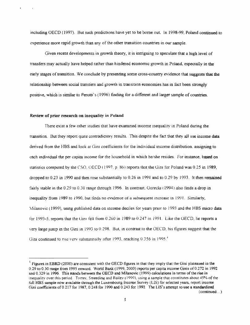
including OECD (1997) . But such predictions have yet to be borne out . In 1998-99, Poland continued to

experience more rapid growth than any of the other transition countries in our sample .

Given recent developments in growth theory, it is intriguing to speculate that a high level o f

transfers may actually have helped rather than hindered economic growth in Poland . especially in the

early stages of transition . We conclude by presenting some cross-country evidence that suggests that th e

relationship between social transfers and growth in transition economies has in fact been strongl y

positive, which is similar to Perotti's (1996) finding for a different and larger sample of countries .

Review of prior research on inequality in Poland

There exist a few other studies that have examined income Inequality in Poland during th e

transition . But they report quite contradictory results. This despite the fact that they all use income data

derived from the HBS and look at Gini coefficients for the individual income distribution, assigning to

each individual the per capita income for the household in which he/she resides . For instance, based on

statistics computed by the CSO . OECD (I997 . p . 86) reports that the Gini for Poland was 0 .25 in 1989 ,

dropped to 0 .23 in 1990 and then rose substantially to 0 .26 in 1991 and to 0 .29 by 1993 . It then remained

fairly stable in the 0 .29 to 0 .30 range through 1996 . In contrast . Gorecki (1994) also finds a drop i n

inequality from 1989 to 1990 . but finds no evidence of a subsequent increase in 1991 . Similarly,

Milanovic (1999), using published data on income deciles for years prior to 1993 and the HBS micro dat a

for 1993-5 . reports that the Gini fell from 0 .260 in 1989 to 0 .247 in 1991 . Like the OECD, he reports a

very large jump in the Gini in 1993 to 0 .298 . But, in contrast to the OECD. his figures suggest that th e

Gini continued to rise very substantially after 1993. reaching 0 .356 in 1995 .4

4Figures in EBRD (2000) are consistent with the OECD figures in that they imply that the Gini plateaued in the

0 .29 to 0 .30 range from 1995 onward . World Bank (1999, 2000) reports per capita income Ginis of 0 .272 in 199 2and 0 .329 in 1996 . This stands between the OECD and Milanovic (1999) calculations in terms of the rise i ninequality over this period . Torrey. Smeedin g and Bailey (1999), using a sample that constitutes about 45% of th efull HBS sample now available through the Luxembourg Income Survey (LIS) for selected years, report incom eGini coefficients of0 .217 for 1987, 0 .248 for 1990 and 0.243 for 1992 . The LIS's attempt to use a standardized

(continued . . . )

5

To summarize. all three studies suggest that income inequality declined from 1989 to 1990. The

CSO-OECD figures Imply a very large increase in income inequality in 1991, while the Milanovic an d

Gorecki figures do not show this . The CSO-OECD (1997) and Milanovic (1999) figures are consistent ,

however, in implying that large increases in inequality occurred between 1992 and 1993 . But the CSO-

OECD figures indicate that inequality then stabilized ., while the Milanovic figures imply that it gre w

substantially again in 1994-95 .

What can account for this wide divergence in reported results? A problem with the studies cited

above is that they do not all use the actual HBS micro data for the period prior to 1993 . Rather, for the

period prior to 1993 . the Gini values in the studies cited above were approximated using aggregate data

on quantiles of the income distribution published by the CSO in the annua l

publication Budzety Gospodarstw , which we henceforth refer to as the Surveys: The accuracy of thes e

approximations is certainly an issue .

But a more serious problem is that in 1993 the CSO switched from quarterly to monthly data

collection . Since income is typically more variable at the monthly than the quarterly frequency, this shift

alone would have created a substantial increase in cross-sectional income inequality and in the Gini

coefficient . Below we will argue that the switch to monthly income reporting accounts for most of the

increase in inequality between 1992 and 1993 reported in both OECD (1997) and Milanovic (1999) .

In the Appendix. we develop a technique for adjusting the 1993-1997 income and consumptio n

data for the increased variability that may be attributable solely to the shift from quarterly to monthl y

reporting . The basic idea of our approach is to assume that income consists of a permanent or predictabl e

definition of income across country surveys could account for part of the difference between their results and thoseof other authors and the CS O

- The Surveys report the number of households in each of several per capita income ranges, along with the averageper capita income within each range, and the average number of persons per household within each range . Thenumber of income ranges reported differs by year . This difference in reporting may itself account for some changein the Gini over time Also, as described below, the income definition used by the CSO included some inappropriat eitems, and in some years the CSO made adjustments for family size, but this was not done consistently over time .

6

component (determined by education, age and other observable characteristics of household members )

plus a mean zero idiosyncratic component . We then assume that the variance of the idiosyncrati c

component would not have jumped abruptly between the fourth quarter of 1992 and the first month o f

1993 . Rather, we assume that the variance of the idiosyncratic component varies smoothly over tim e

(measured in months) according to a polynomial time trend . We estimate this polynomial trend, along

with a dummy for post-1992 that captures the discrete jump in variance that occurred with the change to

monthly income reporting . Then, at the individual level. we scale down the idiosyncratic component of

the post-1992 income data to eliminate this jump in variance .

Another potential problem with previous studies is that the aggregate income statistics reporte d

by the CSO. as well as those repotted by other former communist countries, differ in a number of

important ways from economically meaningful measures of income . The official statistics appear to

reflect total revenues or "inflows" since they include loans. dissaving, and cash holdings at the beginning

of the survey period . For farmers, income includes gross . rather than net. farm revenues . This is an

important issue as approximately one-fifth of Polish households are either farm households or mixed

worker-farmer households . Access to the micro data enables us to make important adjustments in orde r

to obtain a more meaningful measure of income (by excluding non-income revenue items and b y

calculating net farm income) .

' It is possible to make some (but not all) of the necessary adjustments to income using information in the aggregat e

data on categories of income . Inconsistencies in the set of adjustments actually made may account for some of th ediscrepancies in Gini values reported in previous studies .

In a similar vein, the aggregate consumption figures published by the Polish CSO . as well as by other formercommunist countries, often do not correspond to Western-style measures of consumption . Rather, they correspondto a measure of total outflows, including saving and repayment of loans . For farm households, consumptio nincludes farm investment and purchases of supplies. An indication of the strange nature of the aggregateconsumption data is provided by Milanovic (1998, p . 41), who reports that in 1993 the Gini for consumption is 0 .31 ,which substantially exceeds the Gini of 0 .28 for income. He also reports that in 1993 the ratio of consumption toincome is 1 .30, an unreasonably high figure . Our access to the detailed micro data enables us to make necessar yadjustments to the categories that are included in consumption . We then find the more plausible results thatconsumption Ginis are smaller than income Ginis and that the aggregate consumption to income ratio falls in th e0 .89 to 0 .96 range during the 1985–97 period .

7

Both our procedure for adjusting for the spurious increase m inequality stemming for the switc h

to a monthly reporting interval, and our corrections for the definitions of income and consumption . rely

on access to the HBS micro data. In particular, the variance correction requires access to the data for an

extended period of time . Our study is unique in that it is based on the HBS micro data for a long sampl e

period., extending from five years prior to the "big bang" to eight years after . To our knowledge, no prio r

study of inequality in Poland has adjusted for the change in survey design in 1993, and most have not

adjusted for the definitional problems noted above .

Of the several improvements we make over previous studies (use of micro data for the pre-1993

period, correction of the income definition, and adjustment for the switch to a monthly sampling frame i n

1993), it is our adjustment to the change in sampling frame to 1993 that has the greatest effect . We will

argue that failure to account for this change caused prior studies to greatly overstate the increase in

inequality in Poland. In fact, this adjustment is central to our finding that Poland has had the least increase

of inequality of any transition country

The Household Budget Survey s

The CSO has been collecting detailed micro data on household income and consumption at leas t

since 1978, using fairly sophisticated sampling techniques . In the HBS. the primary sampling unit is the

household. A two-stage geographically stratified sampling scheme is used, where the first-stage samplin g

units are the area survey units and the second-stage units are individual households . Households were

At the time we began our study, the Polish CSO had never before released the HBS micro data. A lon gnegotiation process by the first author duri n g 1992—93 led to its release . Subsequently . the micro data for the firsthalf of 1993 was released to the World Bank and this data is used in World Bank ( 1995) and Milanovic (1998) .

More recently, the data for 1993-96 have been obtained by researchers at the World Bank . A subsample of the HB Sis also now available through the Luxembourg Income Survey (LIS) for 1987, 1990 and 1992 . Thus, no priorresearchers have had access to the micro data for the entirety of the extended period that we examine .

The sampling scheme was designed to obtain a survey sample that was representative of the underlyin gpopulation. But the non-response rates differed across demographic groups, necessitating the use of samplin gweights in order to achieve representativeness . We used sampling weights in our analysis where appropriate bu tthese made little difference to any of the main results .

8

surveyed for a full quarter (until 1992) or for a full month (from 1993 onward) in order to monitor thei r

income and spending patterns . Supplementary information on household demographics . durable good

holdings, etc . is collected from the same households once every year . The typical sample size is about

25,000 households per year . The CSO uses the data obtained from these household surveys to create

aggregate tabulations that are then presented in the monthly and annual Statistical Bulletins, or Surveys .

The HBS contains detailed information on sources and amounts of income for both household s

and individuals within each household. Total income is broken down into four main categories : labor

income (including wages, salaries and nonwage compensation) ; pensions ; social benefits and other

transfers; and other income . Social benefits include income from unemployment benefits that were

introduced in late 1989 . A key point is that the data include measures of the value of in-kind payment s

from employers to workers, which have been an important part of workers ' compensation in Poland and

other transition economies . For farm households . farm income and expenditures . as well as consumptio n

of the farm's produce. are also reported. There were no taxes on personal income until 1992 . After that

year, we use net incomes in the analysis .

In addition to the income data the HBS also contains very detailed information on consumption .

For this study, we aggregate the consumption information and only examine household total consumptio n

and total nondurables consumption . Finally. the HBS also contains information on characteristics of the

dwelling, stocks of durables, and demographic characteristics of all household members .

In the immediate aftermath of the big bang, Poland experienced rapid inflation and substantia l

relative price changes . Using information from various CSO publications and IMF data bases, we hav e

extracted quarterly and . for 1993-9 monthly time series on prices that we use to deflate the income an d

consumption data . Our ability to match the frequency of the price data to the frequency of the survey dat a

on income and consumption is important in the context of the large absolute and relative price change s

that occurred during the transition .

Two important changes were made to the HBS survey design in 1993 . We have already noted th e

change to monthly income and consumption reporting . The other major change was an attempt to obtain

a more representative sample of the self-employed . This group's size is believed to have increased

markedly since the transition began, resulting in its under-representation in the HBS data during the

period 1990-92 . In the next section. we examine the extent to which under-representation of the self -

employed may have led to understatement of the extent of inequality in the early years of the transition .

Table 1 (at the end of this paper) reports sample means for some of the variables used extensivel y

in our analysis of inequality .10 Two interesting features are that the average share of income fro m

transfers and the share of pensioner-headed households increase markedly after the transition . We discuss

this in greater detail below. The demographic characteristics of households and household heads remain

quite stable during and after the transition . The means of the education dummies indicate a small increase

in average levels of educational attainment or household heads in the 1990s (a similar increase occurs i n

the general population as well) .

Inequality

In this section . we examine various aspects of inequality in Poland over the period 1985-1997 .

For the years 1993-1997, we use the income and consumption measures that are adjusted (using th e

procedure described in the Appendix) for the increase to idiosyncratic variance that occurred with th e

shift to a monthly reporting period .

The measures of inequality we examine are based on the distribution of individual income o r

consumption, unless explicitly noted otherwise . .A key problem in inequality measurement is ho w to

account for household composition and household economies of scale when measuring household well-

being, or when assigning individual income or consumption levels to household members . Most prior

studies of income inequality in Poland and other transition economies have ignored these issues and

10 Note that the sample size falls in 1992 In that year, half of the total sample was used to test the new monthl ysurvey; these data were considered unreliable and not made available to us .

1 0

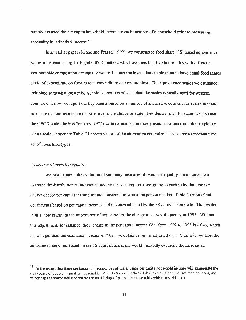
simply assigned the per capita household income to each member of a household prior to measurin g

inequality in individual income .

In an earlier paper ( Keane and Prasad- 1999), we constructed food share (FS) based equivalenc e

scales for Poland using the Engel (1895) method, which assumes that two households with differen t

demographic composition are equally well off at income levels that enable them to have equal food shares

( ratio of expenditure on food to total expenditure on nondurables) . The equivalence scales we estimated

exhibited somewhat greater household economies of scale than the scales typically used for wester n

countries . Below we report our key results based on a number of alternative equivalence scales in orde r

to ensure that our results are not sensitive to the choice of scale . Besides our own FS scale, we also use

the OECD scale, the McClements ( 1977) scale ( which is commonly used in Britain), and the simple pe r

capita scale . Appendix Table B I shows values of the alternative equivalence scales for a representative

set of household types .

Measures of overal l inequality

We first examine the evolution of summary measures of overall inequality . In all cases, we

examine the distribution of individual income or consumption), assigning to each individual the per

equivalent (or per capita) income for the household in which the person resides . Table 2 reports Gini

coefficients based on per capita Incomes and incomes adjusted by the FS equivalence scale . The results

in this table highlight the importance of adjusting for the change in survey frequency in 1993 . Without

this adjustment for instance . the increase in the per capita income Gini from 1992 to 1993 is 0 .045, which

is far larger than the estimated increase of 0 .021 we obtain using the adjusted data . Similarly, without the

adjustment, the Ginis based on the FS equivalence scale would markedly overstate the increase i n

11To the extent that there are household economies of scale, using per capita household income will exaggerate the

'.veil-being of people in smaller households . And. to the extent that adults have greater expenses than children, us eof per capita income will understate the well-being of people in households with many children .

1 1

inequality that occurred between 1992 and 1993 (i .e. . a Gini increase of 0 .046 vs . 0 .018). We use

adjusted income and consumption measures for 1993-97 in all of the remaining analysis .

We also examine the Ginis with adjusted income but excluding the self-employed in 1993-96 .

The inclusion of the self-employed makes only a small difference to either set of Ginis and suggests tha t

under-representation of the self-employed in 1990-92 is unlikely to have resulted in a significan t

downward bias in Gini coefficients for those years . ' 2

The appropriate way of treating the self-employed so as to maintain maximum comparability o f

the inequality measures over time is a difficult issue . For purposes of comparing two adjacent years like

1992 and 1993 . it is probably best to exclude the self-employed. since their fraction of the populatio n

changed little in that short interval . But . for purposes of comparing the degree of inequality in 1997 wit h

years prior to the big bang, it is best to Include the self-employed . since the increase in the number of self-

employed over that period is quite si gnificant and could be an important source of increased inequality .

Henceforth we focus on results includin g the self-employed, recognizing that this generates a bit of a

spurious jump in inequality in 1992- 93 due to the slight change in sample composition .

Table 3 first reports Gini coefficients based on four alternative equivalence scales . Note that the

three scales that account for household economies of scale FS . McClements, OECD) produce very

similar Ginis, typically differing only in the third decimal place . The Ginis based on all four scale s

indicate that inequality increased in 1989 compared to the level in 1985-88, but that inequality returned to

pre-transition levels in 1990 . and continued to decline in I991-92 . The Gini based on the FS scale shows

the sharpest decline in inequality in 1989-92 (from 0 .263 to 0 .230) and the Gini based on per capita

income shows the smallest decline (from 0 .278 to U .2641. but Ginis based on all four scales exhibit the

same basic pattern .

Since this group covers household heads engaged in a wide variety of businesses, households in this group do notsystematically have higher income levels than the sample averages . In fact, the distribution of income among th eself-employed is just slightly more unequal than for the general population .

1 2

In short, inequality spiked up in the immediate aftermath of the big bang but, by 1992, was no

higher than the levels seen before the transition . Starting in 1993, however, inequality began to rise and ,

by 1997, was at a level higher than the peak attained in 1989 . This pattern is robust to the choice o f

equivalence scale . It is important to note, however, that the increase in inequality even by 1997 wa s

hardly dramatic . For example, using the FS equivalence scale, the Gini rose from 0 .256 in 1988 (the year

before the transition) to 0 .276 in 1997 . This increase of 0 .020 is smaller than the increase of 0 .03

reported for the U .S. in the 1980s by Atkinson. Rainwater and Smeeding (1995), or the increase from

0 .326 to 0 .361 reported for the United Kingdom from 1986 to 1991 in World Bank (1999, 2000) .

Conventional wisdom suggests that inequality rose much more in Poland than our results suggest .

All of our Gini coefficients, regardless of the equivalence scale on which they are based, imply a muc h

smaller increase in inequality than is implied by official CSO-OECD (1997) figures for 1989-96 on which

the conventional wisdom about the sharp increase in inequality after the transition appear to be based .

Those figures imply that the Gini coefficient for per capita income rose from 0 .249 in 1989 to 0 .290 in

1993 . ln the same period. our per capita Ginis are rather flat_ rising only from 0 .278 to 0 .282 . For 1996 .

the OECD reports a Gini value of 0 .300 while our value is 0 .301 . During 1989-1996 (the longest period

for which we can compare results), the OECD figures imply an increase of 0 .051 while our figures imply

an increase of only 0 .023 . Thus, while the OECD figures imply an increase in inequality in Poland durin g

the transition that is very large by historical standards, our figures imply an increase that is substantiall y

smaller . Furthermore, our results using the FS scale, which we consider more reliable, imply essentiall y

no increase in inequality over the 1989-1996 period (i .e ., the Gini changes from 0 .263 to 0.265).13

Note that, in the 1990s, our Ginis are closer to those computed by the CSO . In an earlier paper (Keane an dPrasad, 1999), we described a detailed attempt we made to reconcile our Gini coefficients for earlier years with th eCSO-OECD figures, which are also purportedly based on the HBS data . We did not succeed completely . Thedifferences can, to a large extent, be atttibuted to (i) the CSO's use of "revenues" rather than incomes in earlieryears ; (ii) use of grouped data in calculating Ginis (in the 1980s, tabulated decile groups were used, with al lindividuals in a given decile group being ascribed the mean income level within that decile--in recent years ,percentile groups have been used) ; and (iii) the apparent inconsistent use of equivalence scales over time (this i sbased on private correspondence with the CSO) .

1 3

We also examined inequality based on income net of transfers (Table 3, row 5) . 14 Interestingly ,

this reveals a very different picture . The Gini coefficient for income excluding transfers increased b y

0 .066 from 1988 to 1997, more than three times the increase in the Gini for overall income . Thus, it

appears that transfers played a crucial role in inequality dynamics after the transition . We investigate thi s

in greater detail below.

Rows 6-10 of Table 3 report results for consumption inequality (using, as noted earlier, adjusted

consumption data for 1993-97) . Consumption is a better measure of welfare than income, particularly as

measures based on income could overstate inequality since they may reflect idiosyncratic income shock s

that could be smoothed by households . .As expected. the Gini coefficients for nondurables consumptio n

are lower than those for income . Nevertheless . independent of the choice of equivalent scale . they show a

pattern of changes in inequality almost identical to that based on income . Using total consumptio n

reveals a similar picture .

We wished to examine whether our main results were sensitive to the choice of inequalit y

measure. It is well known that the Gini coefficient is particularly sensitive to changes in a distribution

near the median (see Atkinson . 1970). The coefficient of variation (CV) (and its monotonic transforms ,

one of which we use here) is more sensitive to changes at the high end of a distribution. while the mean

logarithmic deviation is more sensitive to changes near the low end . We report these inequality measures

in the bottom 6 rows of Table 3 . in order to determine if they tell a consistent story . In fact, they do.

When we use either income or nondurables consumption, both these measures of inequality also show an

upward spike in 1989, followed by a decline in 1990-92 to below the pre-transition level, and a

subsequent steady increase in 19Q3-97 to a level modestly above that in the pre-transition period .

When we look at income net of transfers, both the coefficient of variation and mean logarithmi c

deviation show far greater increases in inequality over the transition period than for total income . This

14Since transfers tend to be stable over time, the adjustment factors (used to adjust for the change in surve y

frequency in 1993-96) for income net of transfers were nearly identical to those we computed for income includin gtransfers .

1 4

pattern is particularly interesting in the case of the CV measure, which is most sensitive to changes at th e

high end of the distribution. This result stems from the fact that transfers in Poland are focused not onl y

at the low end of the income distribution but extend well into the high end . We give more details on the

targeting of transfers below .

To summarize, we find no evidence to support the view, based on official statistics, of a sharp

increase in total income inequality following the transition in Poland . Rather, we find that the increase in

income inequality was modest compared, for instance, to increases observed in the U .S . and the U.K . in

the 1980s and 1990s . Our results also differ markedly in terms of the timing of changes in inequality .

The OECD-CSO figures imply that inequality grew tremendously from 1989 to 1993, and that it then

stayed rather flat through 1996 . Our results indicate that inequality actually fell from 1989-1992 . But we

find that inequality rose noticeably after 1993 and, especially, in 1996 and 1997 . Thus, we find that mos t

of the increase in inequality occurred several years after the "big bang," and long after the OECD-CS O

figures imply the increase had already ceased .

This difference in timing has important implications for the interpretation of what occurre d

during the transition . The OECD-CSO figures for Poland, as well as the comparable figures for all othe r

transition economies (e.g., Milanovic. 1999), are often interpreted as evidence that substantial increases i n

inequality are an inevitable concomitant of the process of transition to a market economy . Our results,

however, indicate that the change in inequality during the first seven years of the transition in Poland wa s

quite modest . Thus, our results suggest that changes in inequality during transition may not be inevitabl e

but, rather. may result from particular policy choices . In later sections of the paper . we discuss in greate r

detail the role of social transfer policies in inequality dynamics.

Note that our results concerning the evolution of inequality over time were not at all sensitive t o

the choice of a particular equivalence scale . Hence, we use only the FS scale in all further analysis. 15 To

15 We recomputed many of the later results in the paper using different equivalence scales . Although the levels ofinequality were slightly affected by the choice of equivalence scale, as is the case in Table 3, patterns of th eevolution of inequality over time were robust to this choice .

1 5

this point, we have focused on the Gini coefficient and other summary measures in order to compare ou r

results with those of other authors and the CSO . We now exploit our access to the micro data to provide a

richer characterization of the evolution of inequality in Poland.

Quantile ratios and shares

In this section, we examine income inequality by looking at quantile ratios and shares .

Unlike the scalar inequality measures considered in section 4 .I, examination of quantiles allows one to

consider changes in inequality at various different points in the distribution . Figure I plots the 90-10 and

75-25 quantile ratios for each year over the sample period . The quantiles for individuals were calculated

using real household income and nondurable consumption . both adjusted using the FS equivalence scale .

The quantile ratios reveal some interesting patterns . After a brief spike in 1989 . the 90-10 quantile rati o

fell back to its pre-transition level before gradually increasing in the mid-1990s . However, note that the

cumulative increase in the 90-10 ratio from the period 1985-88 through 1997 is only about 0 .20, hardly a

substantial increase . To put this in perspective . Gottschalk and Smeedin g (1997) report a much greater

increase of 1 .04 (from 4 .75 to 5 .79) in the 90-10 ratio for the U .S . from 1980 to 1990 .

The 90-10 ratio for consumption follows a pattern very similar to that of the income ratio over th e

period 1988-97 (although, for reasons that are not clear . It exhibits an upward trend prior to th e

transition) . The 75-25 quantile ratios for income and consumption are essentially unchanged over the

sample period, indicating even great . stability in the middle part of these distributions . We also

examined finer breakdowns of the 90-10 and 75-25 quantile ratios (e .g ., the 90-50 and 50-10 quantiles

ratios) and found that inequality was equally distributed above and below the median and that there were

no significant changes in patterns of inequality that could be detected using these finer breakdowns of th e

data .

Table 4, which reports the shares of income and consumption going to each quintile of th e

respective distributions, provides an alternative perspective . The shares of income, total consumption, an d

nondurables consumption going to individuals in different quintile ranges have remained remarkably

1 6

stable over time, except for a slight and transitory improvement in the relative position of the botto m

quintiles right after the big bang. The evolution of income net of transfers is, however, dramaticall y

different. The total share going to the bottom two quintiles fell from over 15 percent in 1985-7 to 13 . 3

percent by 1992 and further to 10 .7 percent by 1997 . This was mirrored by an increase in the share of the

top quintile, from about 41 percent in 1985-87 to over 46 percent by 1997. These results confirm that

transfers played an important role in the dampening of potential increases in inequality during the

transition, especially at the lower end of the distribution .

Kernel density estimates of income and consumptio n distributions

To obtain a visual representation of changes in the shape and features of the entire distribution ,

we now examine kernel density estimates of household income and consumption distributions . Figure 2

(top panel) presents kernel density estimates for real household income for the years 1988, 1992, 199 3

and 1995 . 16 The density is calculated at the same 200 income points for all four years, and the first 12 5

are plotted in the figure . This covers at least 98% of the households in all four years . Figure 4 (lower

panel) also contains kernel density estimates for real household nondurable consumption for the same

four years . Reflecting the more compact distribution of consumption . the first 75 points cover more than

99% of the households .

The change in the shape of the densities between the year 1988 and selected years after the bi g

bang is striking. Much of the change simply reflects the decline in mean income and consumption

following the big bang . However, the change in shape observed in Figure 2 is not due simply to a

contraction of the mean. To see this . consider taking the distribution for 1991 and multiplying all of th e

income figures by the ratio of mean income in 1988 to that in 1991 . Such a transformation will preserve

relative inequality measures, while equating mean income in 1991 with that in 1988 . This enables us to

1 7

16 An Epanechnikov kernel with a bandwidth of 4000 was used for the kernel density estimation. No adjustmen t

was made for household size .

directly compare the shapes of the distributions . abstracting from mean differences . The 1988 incom e

density and the transformed densities for 1991 and also for 1995 are plotted together in Figure 3 (th e

vertical lines indicate the mean) .

The most prominent features of Figure 3 are that, in moving from 1988 to 1991 . the mass in the

left tail is reduced, and the distribution becomes more peaked around the mode . This accounts for the

declines in the Gini measures noted in Section 4 .1 . A key aspect of what happened during the transition

becomes apparent if one compares the top panels of Figures 2 and 3 . In Figure 2, we see that, as the

overall income distribution shifted left there was a support area at about 34 to 58 thousand zlotys (price s

indexed to 100 in 1992Q4) below which household income tended not to fall . Because of the drop in

mean real income from 1988 to 1991 . the ratio of this support level to mean income increased. In Figure

3 . this has the effect of shifting to the right the fat part of the left tail of the scale-adjusted incom e

distribution .

We investigated the income sources of households with real income in the 34 to 58 thousand

zloty range. and found that these households recei v e over 80% of their income from pensions (80 .5% in

1988 . 82.2% in 1991) . These percenta ges drop off quickly as household income rises above the 5 8

thousand zloty level . The percentage of total household income for all households coming from pension s

was 16 .8% in 1988 and 26 .8% in 199I . Thus, the households with income in the support area of about 34

to 58 thousand zlotys got a far higher share of income from pensions than the typical household .

Furthermore . It is important to note that . while mean real household income fell from 178969 zloty i n

1988 to I31563 zloty in 199I, the mean real pension actually rose from 29811 to 35258 . This resulted

from legislation that took effect in 1991 that made pensions substantially more generous . Hence, it i s

clear from our results that the new pension law helped shift the fat part of the left tail of the income

distribution to the ri ght and that this contributed importantly to the reductions in inequality measures that

1 8

we have noted .17 The lower panel of Figure 3, which compares the adjusted distributions for 1991 and

1995, shows that this effect was further accentuated through 1995 .

Between-group change s in inequality

We have found no evidence of an increase in overall inequality in Poland m the immediate

aftermath of the big bang, regardless of which of several inequality measures we consider . However, thi s

does not mean that there were not winners and losers in the transition . We now turn to an analysis of how

different groups fared in terms of relative income and consumption .

Figure 4 shows how median Income and consumption evolved for four types of household s

differentiated by main income source of the household head : workers, farmers . mixed worker-farmers and

pensioners. A notable feature of the results is that the use of equivalence scales is important . The per

capita household income and consumption plots in the top panel suggest that pensioner-heade d

households moved from a middle position to being clearly better off than other households after the bi g

bang. According to Milanovic (1998 . p . 49), who looked at per capita income . " . . .pensions thus

contributed strongly to increase inequality . '

But the per equivalent unit results in the lower panels tell a very different story . s They indicate

that pensioner-headed households had much lower median income and consumption than other groups

during the 1985-89 period, and that their relative position improved dramatically after the big bang so a s

to bring their income and consumption up to almost the same level as the next lowest group (farmers) . As

17 It is also worth noting that the fraction of households headed by pensioners (and other social benefit recipients )

increased from about 28% in the 1985-89 period to 36% in 1992 . Opting for the more generous pensions wasapparently an attractive option for workers who did not fare well in the transition . We return to this issue later .

18 The reason for the difference in the scales is that the mean numbers of persons in worker, farmer, worker/farmerand pensioner households are 3 59 . 3 o4 . 4 55 and 1 88 respectively. while the mean numbers of equivalent units ar e

1 .69, 1 .77, 2 .08 and 1 .19 respectiveł y .

1 9

a result, we find that pensions contributed importantly to a reduction in inequality . ' The main impetus

behind the improved relative position of pensioners was a substantial increase in pension levels that too k

place in 1991 . In fact, by 1997 . the relative position of pensioner-headed households was inferior only t o

that of worker-headed households .

We also examined the fractions of households that fall in each quintile of the income distribution ,

conditional on education or age of the household head (results not shown here) . One main finding was

the substantial improvement in the relative positions of households whose heads have higher educational

qualifications . For example. in 1989, 45 .8% of households in which the head had a colle ge degree were

in the top quintile . This fraction rose to 58% by 1992 and further to 60 .2% by 1997 . By contrast, i n

1989. among households in which the head had only a primary school education . 14 .9% were in the to p

quintile . but this had fallen to 9 .5% by 1992 and to 8% by 1997 .-mother striking result was th e

improvement of conditions for the old, which resulted from more generous pensions . Among household s

in which the head was over 60 years old, 392% were in the bottom quintile in 1989, but this dropped t o

only 24 .3% by 1992 . ln contrast_ the probabilities that a household with a young (18-30) or middle age d

(31-60) head would fall in the bottom quintile of the income distribution increased over the same period .

Within-group changes i n inequality

In this section. we address the question of the extent to which inequality is within vs . between

group, and the extent to which each type of inequality changed over the transition . The single paramete r

generalized entropy measures of inequality can be additively decomposed into within- and between-group

components (see Shorrocks . 1084) . This family includes the mean log deviation and half the square o f

the coefficient of variation. but not the Gini coefficient . Hence, in the top panel of Table 5, we report

decompositions of the former two inequality measures for income, grouping individuals by the mai n

19 In a result that echoes ours . Garner and Terrell (1998) find that pensions substantially reduced inequality (asmeasured by income Gini coefficients) during the early transition years in the Czech and Slovak republics .

2 0

income source of the household head . Notice that the vast majority of inequality is within group, rather

than between group, which is not surprising given the coarse nature of the grouping . Both measures

indicate that most of the increase in inequality during the transition was within group .

An interesting finding, which is apparent in the second panel of Table 5 . is that the changes in

within-group inequality were very different across different groups . For instance, Gini coefficients

estimated separately for each group indicate a steady rise in inequality for individuals in worker-headed

households, from 0 .189 in 1988 to 0 .248 in 1997 . This increase of 0 .059 in the Gini for individuals in

worker-headed households is almost three times as great as the 0 .020 increase in the Gini for the overall

income distribution . The Gini coefficients in Table 5 indicate that within-group inequality actually fell

among farmer and mixed worker-farmer households during the transition . There was also a modest

increase in inequality within pensioner-headed households .

The most striking result here is the significant and steady increase in inequality among worker -

headed households after 1988 . The bottom two rows of Table 5 reveal that much of the increase in

income inequality among worker-headed households can be attibuted to increased inequality in labo r

income. When we look at labor income alone, the Gini increased from .252 in 1988 to .298 in 1997, an

increase of .046 . Thus, we see that inequality in labor earnings grew substantially more than inequality i n

the overall income distribution .

It is interesting to examine how overall income levels of worker-headed households wer e

influenced by the human capital attributes of the household head . We ran quantile regressions of log rea l

household income on characteristics of the household head (and an urban dummy) . We do not report the

results in detail here but only briefly summarize the main findin gs. Log incomes for households wit h

heads in all education groups drop substantially at all quantile points from 1989 to 1990 ; these decline s

are greater at the upper quantile points, implying a slight reduction in within-education group inequality .

However, by 1992, there is a clear divergence across groups . Households with a college-educated head

experience a recovery in income : those with a high school-educated head have stable real incomes at mos t

quantile points ; and households headed by persons with lower educational qualifications experience a

continuing decline in income . This divergence across groups is accentuated during 1994-96, confirmin g

the earlier results that indicated rising inequality among worker-headed households after the transition .

Earnings inequality

In order to gain more insight into the sources of changes in labor earnings inequality, we also

examined the evolution of earnings for individual workers . These data are available in the HBS for all

years except 1993 and 1997 . We analyzed changes in the wage structure using OLS and quantile

regression techniques . To conser v e space. we do not present those results here but only briefl y

summarize the main findings that are relevant to this paper .

The most prominent result in the wage regressions was the sharp increase in education premi a

after the transition. Estimates of standard human capital earnin gs functions (see . e .g., Willis, 1986)

indicated that the earnings premium for a college degree relative to a primary school degree increased

from 47% in 1987 to I02% in 1996 . The high school premium increased from 23% to 45% over the same

period. These figures are also reflected in our earlier comments about the greater representation o f

households with better-educated heads in the upper quantiles of the income distribution as the transition

progressed .

Our finding of a sharp Increase in education premia after the transition is consistent with that of

Gorecki (1994) . based on his examination of aggregate Polish wage data, and of authors who have

examined the wage structure in other transition economies . For Instance . Ham. Svejnar, and Terrell

1995) examine surveys conducted by the Federal Ministry of Labor in Czechoslovakia in 1988 and 1991 .

They find that the wage gap between university and elementary school graduates increased from 58% in

1988 to 63% in 1991 . Based on her analysis of Russian data, Brainerd (1998) reports that, from 1991 to

1994, the marginal return to a year of education rose from 3 .1% to 6 .7% for men and from 5 .4% to 9 .6%

for women.

The other main result in our wage regressions was that experience premia are estimated to hav e

declined sharply in the early years of the transition . These declines were quite large at all quantile points

2 2

of the distribution that we examined and were especially sharp for older workers . There was a slight

recovery in experience premia in 1994-96 : this recovery was greater for older workers while, for younge r

and middle-aged workers. experience premia remain below their pre-transition levels even by 19% .

Our results indicate that the returns to general human capital, reflected in education premia, ros e

markedly after the transition while the returns to experience, especially for older workers, decline d

sharply in the early years of the transition . This is consistent with the notion of rapid obsolescence o f

firm- or industry-specific skills during a period of rapid technological change and industrial restructurin g

(see Svejnar . 1996) . Workers with higher levels of general human capital are better able to adapt to suc h

changes, while older workers, who typically have higher levels of firm- or industry-specific huma n

capital, face a sharp decline in their earnings potential . This, combined with the increased generosity o f

pensions . explains the surge in the number of pensioner-headed households in 1991-1992 that we noted i n

Table f . Indeed, self-selection into retirement probably accounts for the recovery in experience premia

for older workers that occurred after 1992 . since a large number of older workers, particularly in the 55 -

65 age bracket. retired in 1991-92 . The patterns of changes in earnings inequality that we have discusse d

here have important implications for understanding key aspects of the political economy of the transitio n

process. This is the subject of the next section .

The targeting of transfers : a political economy perspective

The analysis thus far has indicated that, while inequality in labor earnings did increas e

substantially among workers and worker-headed households, the overall rise in income inequality durin g

the transition was quite effectively dampened by social transfer mechanisms . In this section, we provide a

more detailed examination of the targeting of transfers .

First, we examine the extent to which transfers alleviated poverty . The poverty line is, of course,

a rather arbitrary concept . But there is widespread agreement that the poverty lines developed by th e

Institute of Labor and Social Affairs in Warsaw are "overly generous (see OECD, 1997, p .91 ;

23

Milanovic, 1998, p . 66) . 20 Instead. we calculate poverty lines by first constructing the median of per

equivalent household income using pooled data for the entire 1985-97 period . Then, we alternately define

a household as being in poverty if it has per equivalent income below either one-half or two-thirds of tha t

median. The first panel of Table 6 shows the fraction of the population living in households with pe r

equivalent income below each of those thresholds in each year. For instance, the fraction of th e

population below the one-half median threshold jumped from about 2-3% in 1988-89 to 6% in 1990-92 .

This fraction rose further in 1993 . peaked at 10% in 1994 . and then declined moderately by 1997 . A key

finding is that, while poverty jumped in the immediate aftermath of the big bang, it did not increase much

in the subsequent two years . Poverty rates based on the two-thirds median income threshold are higher

but have the same time profile .

To analyze the targeting of transfers . we first conducted the simple experiment of removin g

transfers from household income and redistributing the transfers equally to all households based on their

number of equivalent units . Such an experiment of course assumes away any behavioral response o f

households to the change in transfer rule, but it does reveal the extent to which transfers alleviate poverty

in a purely accounting sense . In 1992. the fraction of people below the two-thirds median threshold drop s

from 27% to 20% (columns 4 and 2) as a result of transfers . while the fraction below the one-half median

threshold drops from 16% to 6% (columns 3 and 1) . Perfect targeting of transfers would imply that the

percentage below the one-half median threshold should be reduced to zero before the percentage below

two-thirds of the median is reduced at all . Thus, the fact that transfers appear to do less to reduce th e

fraction of people below the one-half median threshold suggests that targeting to the least well-of f

households could have been substantially improved .

ln short, while transfers did mitigate the increase in poverty during the transition, they coul d

clearly have been better targeted if the goal was to prevent an increase in poverty .

20 Using these poverty lines . Szulc (I994, 1995) calculates that the percentage of households in poverty rose from16 .7% in 1989 to 34 .2% in 1990, and further to 40 .3% in 1992 . But the poverty line appears to lose its meaning i nthe local context when such a large fraction of the population is counted as poor .

24

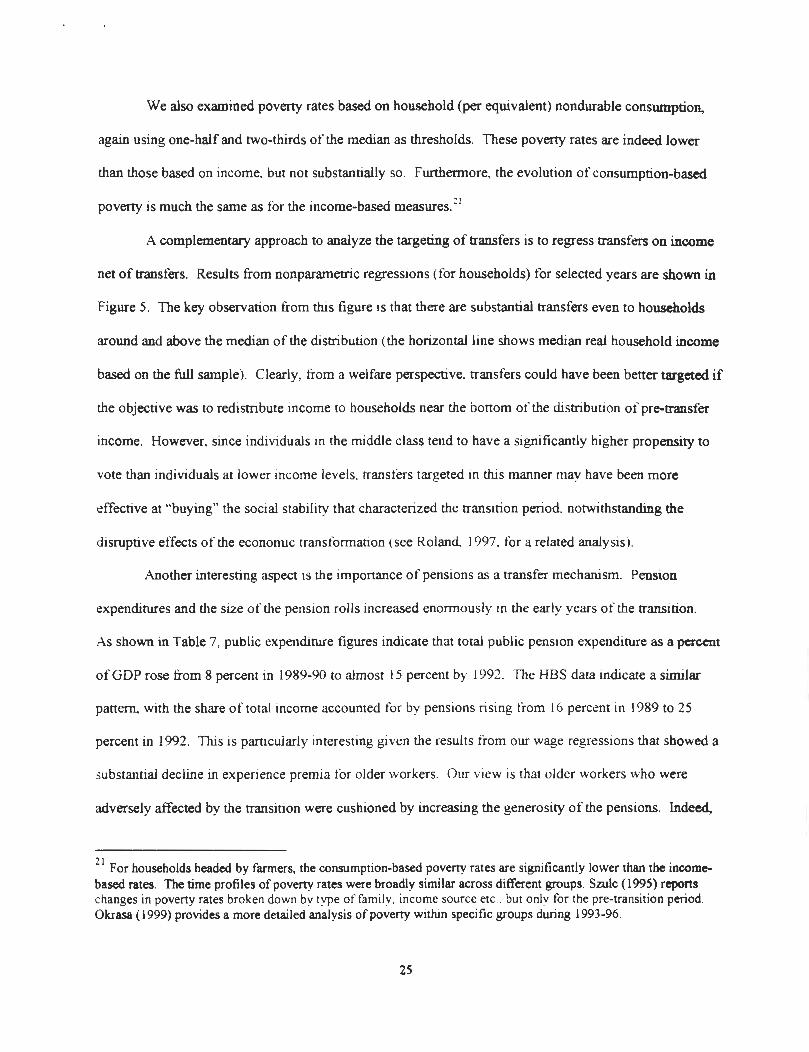
We also examined poverty rates based on household (per equivalent) nondurable consumption,

again using one-half and two-thirds of the median as thresholds . These poverty rates are indeed lower

than those based on income, but not substantially so . Furthermore, the evolution of consumption-base d

poverty is much the same as for the income-based measures .21

A complementary approach to analyze the targeting of transfers is to regress transfers on incom e

net of transfers . Results from nonparametric regressions (for households) for selected years are shown in

Figure 5 . The key observation from this figure is that there are substantial transfers even to households

around and above the median of the distribution (the horizontal line shows median real household income

based on the full sample) . Clearly, from a welfare perspective . transfers could have been better targeted i f

the objective was to redistribute income to households near the bottom of the distribution of pre-transfe r

income. However, since individuals in the middle class tend to have a significantly higher propensity t o

vote than individuals at lower income levels, transfers targeted in this manner may have been mor e

effective at "buying" the social stability that characterized the transition period_ notwithstanding the

disruptive effects of the economic transformation (see Roland. 1997, for a related analysis) .

Another interesting aspect is the importance of pensions as a transfer mechanism . Pension

expenditures and the size of the pension rolls increased enormously in the early years of the transition .

As shown in Table 7, public expenditure figures indicate that total public pension expenditure as a percen t

of GDP rose from 8 percent in 1989-90 to almost 15 percent by 1992 . The HBS data indicate a similar

pattern, with the share of total income accounted for by pensions rising from lb percent in 1989 to 2 5

percent in 1992 . This is particularly interesting given the results from our wage regressions that showed a

substantial decline in experience premia for older workers . Our view is that older workers who wer e

adversely affected by the transition were cushioned by increasing the generosity of the pensions . Indeed,

21For households headed by farmers, the consumption-based poverty rates are significantly lower than the income -

based rates. The time profiles of poverty rates were broadly similar across different groups . Szulc (1995) reportschanges in poverty rates broken down by type of family, income source etc . but on ł y for the pre-transition period .Okrasa (1999) provides a more detailed analysis of poverty within specific groups during 1993-96 .

2 5

the replacement rate (average pension as a ratio of average wage) rose from about 52 percent in 1988-89

to 65 percent in 1991 and remained above 60 percent through 1997 (OECD, 1998) .

Furthermore, since older workers had the most to lose from the privatization or closure of existin g

state-owned firms, giving them the option of moving on to the pension rolls may have been a key factor

in removing a potential political obstacle to enterprise restructuring and privatization . This option,

reflected in a relaxation of the pension eligibility requirements in 1990-91, was indeed exercised by a

large number of workers, resulting in an increase in the number of newly granted pensions from about 0 . 6

million per year in 1988-89 to almost I .4 million in 1991 (OECD . 1998, p . 65) . Consistent with thi s

result, we find that, in the HBS data among households headed by a person in the 55-65 age range, th e

share of labor income in total income declined from 24 percent in 1989 to I2 percent by 1994 . before

recovering somewhat to 16 percent by 1997 In these years, the share of pension income in total incom e

for these households was b4 percent, 74 percent. and 73 percent. respectively.22

Thus. transfers may have contributed not only to social stability but also to ensuring the

conditions necessary for reforms such as privatization and enterprise restructuring that paved the way fo r

high growth after the transition . .As shown in the bottom panel of Table 7, this was accompanied by a

substantial increase in the general government budget deficit in the early years of the transition . Although

there was an attempt to hold the line on transfers in 1990, starting in 1991, the increased generosity o f

pensions and other social benefits led to a mushrooming of the deficit . This proved unsustainable and, by

1993, growth in transfer expenditures (as a percent of GDP) had been halted, although pensions and othe r

social benefits were at a higher level than in the pre-transition years . The increase in aggregate inequalit y

after 1993 is yet another indicator of how important the growth in transfers was in dampening the rise i n

overall inequality in the early years of the transition .

22Among households with heads in the 45-55 age range and in lower age ranges, there was a small drop from 198 9

to 1992 in the share of income from labor income, but this was mostly offset by an increase in other social benefit srather than pensions . Among households with heads aged 65 and older, pensions constitute 85-90 percent of totalincome, with labor income accounting for barely 2 percent .

26

To summarize, the analysis in this paper highlights the role of policy choices, as embodied i n

transfer and other policies, on the dynamics of inequality during the transition to a market economy. In

particular, we have argued that the increase in transfer expenditures ( and. consequently, the budge t

deficit) during the critical early years of the transition may have played an important role in setting th e

stage for the successful economic transition in Poland .

Inequality, transfers and growth : some cross-country evidenc e

Our detailed analysis of the Polish transition experience has suggested that, from a political

economy perspective, the use of transfer mechanisms to mitigate the potential rise in inequality during th e

transition to a market economy may have important implications for the success of the transition process .

In this section. we expand our analysis to provide a cross-country perspective on the experiences of th e

transition economies of Eastern Europe in terms of inequality, social transfers and growth .

.A prerequisite for the investi gation is that we have available for each country two measures of

income inequality : one for a year prior to the start of the transition and a second for a year several year s

after the start of the transition (so that the data do not simply capture the effects of the initial phase o f

transition on inequality) . It is also important that the pre- and post-transition Gini values for each country

be based on similar measures of income, similar sampling time frames, similar data sets, etc ., so that th e

measures are reasonably comparable . Fable 8 reports pre- and post-transition Gini values, obtained fro m

(3 different sources that we believe reasonably satisfy these comparability criteria . The sources ar e

Milanovic (1998, 1999), World Bank (1997 . 1999, 2000) and OECD (1997) .

The Gini coefficients in Table 8 are all for the respective individual income distributions ,

assigning to each individual the per capita income of the household . We have argued earlier that it woul d

be more reasonable to use equivalence scales to accommodate household economies of scale and th e

different consumption needs of children versus adults . But only per capita income Ginis are available for

most transition economies . Ginis based on labor earnings are available for more countries, but these

would not account for the effect of transfers on the distribution of total income, which is our focus .

2 7

Some omissions from the table are noteworthy . We require that post-transition Gini values be in

the 1995-7 period . As a result . we are unable to obtain post-transition values for the Slovak Republic ,

Uzbekistan . Turkmenistan and Moldova . Gini values for these countries are constructed by Milanovi c

(1998) for 1993, but we view this as too soon after the start of the transition for our purposes .

While Gini information for transition countries is scarce, there were 5 cases where we had Gini s

for both 1988 and 1989 and two cases (besides Poland) where we had Ginis for both 1995 and 1996 . In

the former cases we took 1988 (the earlier year) and in the latter cases we took 1996 (the later year) . Also

note that the post-transition Gini values for Lithuania and Kazakhstan are for consumption rather than

income. This probably understates the increase in income inequality in these countries . Since these

countries also had poor growth performance. the effect Is . if anything . to understate the negativ e

correlation between GDP growth and changes m inequality that we find (see below) .

Table 8 reports annualized cumulative GDP growth in the first 8 years of transition . This

corresponds to the 1990-97 period for all eastern European countries except Romania (1991-98) and the

other Former Soviet Union countries (1992-99) . The table also reports the mean level of social (cash )

transfers. as a percent of GDP. averaged over the period from the first year of the transition through 1997 .

Note that Poland and Slovenia are the only countries that surpassed pre-transition levels of GDP after 8

years . These countries also have amon g the hi ghest average levels of social transfers (17 .7% of GDP for

Poland, 14 .8% for Slovenia) .

Finally, Table 8 also reports two variables that could be relevant for explaining the differen t

growth experiences of the transition economies . The first is a summary

measure of the EBRD transitio n

indicators for each country, taken from the EBRD ' s 1 995 Transition Report . This is a measure of

government policies in terms of the degree of transition towards a market economy framework .23, 24. The

The EBRD report contains ten measures of the degree of transition to a market economy . Three of the measuresrelate to enterprises : the degree of large and small scale enterprise privatization, and the degree of enterpris erestructuring (including elimination of soft-budget constraints) . Three measures relate to markets and trade : thedegree of price liberalization, the degree of trade liberał ization and access to foreign exchange, and the extent o fenforcement actions to prevent abuse of market power . Two measures relate to financial institutions : bankin g

(continued . . . )

28

second variable is a measure of the difficulty of the initial conditions facing each country at the start o f

the transition . This variable, taken from de Melo, Denizer. Gelb and Tenev (1997, henceforth MDGT), i s

constructed using factor analysis and is based on the degree of industrialization . extent of initial

macroeconomic imbalances, geographic orientation of trade and length of time under communism. We

report the first common factor from their analysis . A higher score indicates more favorable initial

conditions .25

Figure 6 plots cumulative GDP growth in the first 8 years of transition against the change in th e

Gini coefficient . A strong negative relationship is obvious, with those countries that have experienced th e

best growth performance also having the least increase in income inequality . The simple correlation is -

0 .86 . The bottom panel of the figure also plots the relation between growth and government transfers as a

percent of GDP, for all 18 countries for which we were able to obtain transfer data . The relationship i s

strongly positive . with a simple correlation of 0 .67 (0 .61 in the subsample of 14 countries for which we

have Gini coefficients) . Note that finding a positive correlation between transfers and growth i s

particularly surprising given the blatant denominator bias driving the correlation in the opposite directio n

(higher output growth increases the denominator of the transfer to GDP ratio) . 26 It is interesting that both

reform and interest rate liberalization, and the establishment of securities markets . And two measures capture theextent and effectiveness of the legal framework for securing property rights and regulating business activity . Themeasures are on a scałe of I to 4+ . with I indicating little progress and 4+ indicating a level comparable to that o fwestern industria ł ized countries . We averaged the transition indicators within each of the 4 groupings (scoring a 4 +as a 5), and then averaged across those 4 scores, to obtain an overall measure of liberalization .

,4 We conducted an exploratory regression analysis to see what combination of the EBRD indicators would bes t

explain growth . We tried r e g ressions of cumulative GDP growth in the first 8 years of transition on many differentsummary measures of the ten EBRD indicators . We found that the equal weighting within each of the 4 broadcategories, followed by equal weighting of the four broad categories, produced as good an Rsquared as any othe r

procedure .

25 It is worth noting that this measure is very highly correlated with distance from Western Europe . Thus, by usin gthis variable to explain growth, one risks falling into the vacuous conclusion that the Centra ł Asian countries di dpoorly because they are Central Asian countries . However, it is interesting that Uzbekistan did much better(relatively) than would be expected given its initial conditions, while Bulgaria and Latvia did much worse . We didnot use the second factor from MDGT because it had a negligible partial correlation with GDP growth.

26 Another problem is that higher transfers do not necessarily imply more redistribution . As noted by Commande rand Lee (1998), transfers in Russia have actually become regressive in the transition .

29

of these results that we find here for transition economies have also been reported by authors such as

Perotti (1996) for a different but much larger sample of industrial and developing countries .

These results are at least not inconsistent with recent developments m growth theory which imply

that redistribution to enhance equality may actually enhance rather than dampen growth . But it is of

course possible that some third factor explains both good growth performance and the maintenance o f

income equality in transition economies, and that the correlation we see between growth and the chang e

in inequality has no causal interpretation. To investigate further. we tried regressions of growth o n

changes in the Gini coefficients . along with the EBRD measure of extent of transition to a market

economy framework and the MDGT measure of initial conditions facing each country — the idea being

that the extent of liberalization or the difficulty of initial conditions are plausible omitted factors that

could explain both growth and chan ges in inequality .

These results, reported in Table 9 . indicate that. individually, the EBRD transition indicator, th e

MDGT initial conditions measure . and the changes in the Gini coefficients are all highly significantl y

related to GDP growth (adjusted Rsquareds range from 0 .57 to 0 .72) . In column 4 . we include all three

variables . Interestingly, only the EBRD transition indicator and the Gini difference are significant, whil e

the initial condition indicator is not . This suggests that initial conditions did not matter for growth onc e

subsequent policy choices ( the transition indicators) are controlled for . The results in column 5 confirm

this, since the adjusted Rsquared increases when the initial condition indicator is excluded from the

regression . The coefficient estimates imply that market liberalization is positively associated wit h

growth, while increasing inequality is negatively associated with growth .

Of course. a problem with these results is the potential endogeneity of the change in inequality .

In an attempt to address this problem. in column 6 we instrument for the Gini difference using the initia l

condition indicator. This procedure relies on the (admittedly strong) identifying assumption that initia l

conditions do not directly affect growth once we control for subsequent policy choices (the transition

indicator) . Granted that, in column b we are identifying the effect of inequality on growth through

variation in inequality outcomes that can be attributed to initial conditions differences (as opposed to

3 0

changes in inequality that may have been caused by subsequent growth outcomes) . Interestingly, the

coefficient on the Gini difference does not change much and remains highly significant . In fact, thi s

coefficient is quite stable whether we include initial conditions in the re gression (column 4), use initia l

conditions to instrument for the difference ( column 6), or exclude initial conditions entirely and run OLS

(column 5) .

A coherent interpretation of these results would be that greater progress towards a marke t

economy framework enhances growth but that . conditional on the degree of liberalization, policy that

maintains a greater degree of equality is more conducive to growth . Initial conditions do not affect

growth directly once one controls for policy choices . But initial conditions do seem to matter through

their effects on policy . in particular . countries with better initial conditions have not only made more

rapid progress towards liberalization. but they have also tended to pursue policies that have resulted i n

smaller increases in inequality in the process . Only to the extent that better initial conditions have led t o

more liberalization or more equality have they enhanced growth . Of course, as noted above, thi s

interpretation relies on a strong identifying assumption and other interpretations can not be ruled out .

We are naturally cautious about drawing strong conclusions from I4 data points . But, on the

other hand. note that this is not really a "small sample" but rather the entire population of Easter n

European countries experiencing the transition process (barring a few for which data are not available) .

One might feel we could obtain more conclusive results by exploiting the panel aspect of the data . But

inspection of the data over time reveals that for each country there is tremendous persistence in growt h

performance, as well as in the degree of liberalization and the extent of increase in income inequality .

That is, those countries that have relatively good growth performance. a relatively high degree of

liberalization, and a relatively low increase in inequality tend to remain that way throughout th e

transition, and vice-versa. Thus, we do not feel that there is much to be gained by looking at these data a s

a panel . It would be an illusion to think there are many more than 14 independent observations to wor k

with here .

3 1

Our overall interpretation of these results is that, consistent with the Polish experience that w e

have analyzed in detail in this paper, the use of social transfer mechanisms and other policies to buffer the

potential increase in income inequality . especially in the critical early phase of transition. appears to b e

important in generating a successful transition to a market economy . We have argued that the Polis h

experience points to an interesting example of targeting of transfers that while not necessarily ideal fro m

the perspective of preventing an increase in poverty, may have been crucial for garnering political support

for the drastic market-oriented reforms that facilitated Poland's strong growth performance in the 1990s .

Concluding remarks

This paper has argued, based on detailed analysis of household income and consumption data fo r

the period 1985-97, that . in Poland. there is little evidence of a substantial increase in overall inequalit y

during the transition that began m 1989-90 . This contradicts the conventional wisdom that the process o f

transition to a market economy is inevitably accompanied by a surge in inequality . However, we did find

that earnings inequality among workers increased substantially during the transition . We also

documented that social transfer mechanisms played an important role in dampening the increase in overal l

inequality and in between-group Income dynamics . We argued that. although the structure of transfer s

may not necessarily have been ideal from the perspective of preventing an increase in poverty, transfer

mechanisms may have played a critical role in maintaining social stability and in reducing politica l

resistance to the structural reforms that were undertaken in the early years of the transition and tha t

facilitated Poland's subsequent strong growth performance . Finally, we presented cross-country evidenc e

on inequality, transfers and growth in transition economies that, while not conclusive, is consistent with

the notion that social transfers and other policies aimed at mitigating increases in inequality, especially in

the critical early phase of transition, may be conducive to growth .

3 2

Appendix : Accounting for the change in survey frequency in 199 3

A few important changes were introduced to the HBS in 1993 . Starting in that year, households

were surveyed for only one month rather than for a full quarter . In addition, the sampling scheme was

modified to provide better coverage of the self-employed . Further, police, security and military personnel

were included in the survey. Other aspects of the survey, such as the two stage sampling scheme and the

structure of the survey instrument, were left essentially unchanged .

For the purposes of measuring cross-sectional inequality, the change in survey frequency is th e

most important change . In this appendix, we develop a technique for adjusting the 1993-1997 income an d

consumption data for the increased variability that may be attributable to the shift from quarterly t o

monthly reporting . We begin by assuming the following, -'statistical" or -'forecasting" model fo r

household income :

Yht =alt

3 t -ht - o, E-h t

where Y h , is income of household h in period t . \ h, is a vector of household characteristics used to predic t

household income, and s h , is the unpredictable or idiosyncratic component of household income scaled t o

have a standard deviation of unity The time-specific standard deviation that scales the idiosyncrati c

component of household income Is denoted by a, . Our objective is to estimate the increase in a t for the

1993-97 period that is due solely to the switch to a monthly reporting interval .

We begin by estimating equation l) separately for each quarter from 1985-1992 and eac h month

from 1993-1997 .27 The variables included in X ht, are controls for education level. age and sex of th e

household head, controls for presence of a spouse and age of the spouse. and controls for household size,

urban residence, and primary income source of the household head . While the coefficients on most of th e

controls were stable over time in these regressions . one interesting aspect was that the education of th e

household head became more important as the transition progressed . A key feature of the results was tha t

3 3

27 These results are not reported in the paper but are available from the authors .

the R 2 values dropped sharply after the shift to monthly reporting in 1993 . Presumably, the bulk of thi s

drop is due to greater idiosyncratic variability of income, as well as greater relative importance o f

measurement error, when income is reported at monthly rather than quarterly frequencies .

Next we assume that the standard deviations of the residuals from estimation of equation (1 )

follow the process :

(2)

In 6, =

+ n,t + 12t :

c i t .

?t,,YB, 7 51[t>96] – rlt t = 2, 4 95 ;

t = 97. 98 156 .

Here t is a monthly time index . For the years 1985 through 1992, the data are quarterly, so t is assigned as

the midpoint of the interval covered by each quarter (that is, t = 2 . 4 95) . The variable I[t>96] is an

indicator for the 1993-1997 sample period in which the data is monthly . Thus,

captures the structura l

shift in the error standard deviation attributable to the shift to a monthly data frequency . The time

polynomials capture the evolution of the error standard deviation over tune due to changes in within-

group income inequality, controlling for the group characteristics included in X . The term YB, control s

for the effect of changes in mean income on the error standard deviation . Finally, rp t captures purely

idiosyncratic period-specific chan ges in income variability .

Analysis of the residuals from equation ( 1) indicates that households with different primar y

income sources (i .e ., worker-headed households, farm households, mixed farmer/worker households an d

pensioner households) have very different error variances. as well as different behavior of the error

variances over time . Therefore . we estimate equation (2) separately for each household ripe, using th e

time series of residual variances from (1) .

Estimates of equation (2) for each of the four household types are reported in Table Al, and plot s

of actual and predicted values of the dependent variable In 6, are presented in Figure A I . Observe that

the estimates of 7 5 are largest for farm and mixed farmer/worker households (0 .369 and 0 .201), smaller

for workers (0 .165) and smallest for pensioners (0 .044). This is as we would expect since the increase i n

income variability as a result of switching to a monthly survey period should be lowest for pensioners –

3 4

whose primary income source is very stable from month to month — and greatest for farmers (wit h

workers somewhere in between ) . The plots of the log residual standard deviations from the estimation of

equation ( l) clearly reveal the jump in the error standard deviation that occurs for each group in Januar y

1993 (t = 97) . It is this jump that the coefficients 7 5 on the post-1992 dummy are picking up .

There are a number of other Interesting aspects of the plots in Figure Al . For workers, note the

cluster of large residual standard deviations in the five periods t = 32, 34, 36, 38 . 40, which correspond to

the fourth quarter of 1988 through the fourth quarter of 1989 . There is then a precipitous drop in the

residual variance in the period t = 42 . which corresponds to the first quarter of 1990 . This drop in the

standard deviation is mainly a scale effect, resulting from the sharp fall in real incomes that occurred righ t

after the big bang . The model tracks this drop in the standard deviation well due to the inclusion of th e

mean income level term .

Also note that the error standard deviation appears to rise substantially in 1996-97 for all groups .

But this in itself does not necessarily mean that the within-group income equality began to grow rapidl y

in 1996-97 . Part of the increase is purely a scale effect due to the fact that mean real income levels grew

substantially in Poland in 1996-97 . In Figure A2 (top panel), we plot the polynomial in time alone,

holding YB, fixed at the full sample mean, and setting 1(t ' 06] to zero . These plots indicate tha

t within-group income inequality did begin to grow substantially in 1996-97. even after controlling for changes i n

the scale of real income . Including the time dummy (lower panel) shows the effect of the adjustment o n

within-group residual variances .

Finally, we adjust the income data for 1993-1997 to account for the increase in the idiosyncrati c

variance that we estimate occurred solely due to the shift to a monthly reporting period in January 1993 .

We define adjusted income for the 1993-97 period as :

(3)

YAht = apt + ftX„-ia, / exp(1t5) Eht

t=97.98 156 .

Here E h , is the estimated residual from equation (1) and n5 is our estimate from equation (2) of the

increase in the log of the residual standard deviation due to the switch to monthly income reporting . The

3 5

scale factors exp(It i ) differ for households with each of the four primary income sources . They are 1 .179 ,

1 .446, 1 .222 and 1 .045 for worker-headed households, farm households, mixed worker-farmer an d

pensioner-headed households . respectively .

A problem we confront is that a representative sample of the self-employed was not obtained in

the pre-1993 surveys. Some respondents in the pre-1993 surveys report that they are self employed . But

representation of this group in the pre-1993 data is too small to obtain reliable estimates of the group- an d

time-specific residual variances . Besides, we could not be sure of the extent to which any change i n

variance for this group in 1993-97 is due to the shift to monthly reporting vs . increased representativeness

of the self-employed sample . Thus. we simply assume the same scale factor for the self-employed as w e

do for workers (1 .1 79). In any case . it turns out that our results on changes in inequality are not ver y

sensitive to how we treat the self-employed. because they constitute only about 5-6 percent of the sample .

We also adjust the consumption data using the same procedure we use for income. We do not

discuss those results in detail but simply note that the scale factors exp (r«) for consumption are 1 .108 ,

1 .149 . 1 .118 and 1 .086 for worker-headed households . farm households. mixed worker-farmer and

pensioner-headed households . respectively. As expected . these are lower than the income adjustmen t

factors and are quite similar across different groups . For pensioner households . the jump in consumption

variability is greater than the jump in income variability with the switch to monthly reporting . While

these households have more stable month-to-month income streams than other households, there is n o

obvious reason to expect their month-to-month variability in tastes for consumption to be lower . Finally ,

we adjust the consumption data for the self-employed usin g the same scale factor we used for workers.

3 6

References

Aghion. Philippe and Simon Commander (1999) "On the Dynamics of Inequality in the Transition . "Economics of Transition . Vol . 7 :2, pp . 275-98 .

Aghion, Philippe and Patrick Bolton ( 1997) "A Trickle-Down Theory of Growth and Development wit h

Debt Overhang," Review of Economic .studies . Vol . 64 :2, pp. 151-62 .

Aghion Philippe. Eva Caroli and Cecilia Garcia-Peñalosa (1999) "Inequality and Economic Growth : Th ePerspective of the New Growth Theories ." Journal of Economic Perspectives, Vol . 37:4, pp. 1615 -

60 .

Alesina. Alberto and Dani Rodrik (I994) "Distributive Politics and Economic Growth, " Quarterly

Journal of Economics . Vol . 109 :2 . pp . 465-90 .

Atkinson, Anthony B . (1970) "On the Measurement of Inequality . " Journal of Economic Theory, Vol . 2 ,

pp . 244-63 .

Atkinson. Anthony B . . Lee Rainwater and Timothy M. Smeeding (1995) "Income Distribution in OEC D

Countries : Evidence from the Luxembourg Income Study_ OECD Social Polic y_ Studies No. 1 8

( Pans. France : OECD) _

Banerjee, Abhijit and Andrew F. Newman (1993) "Occupational Choice and the Process o f

Development," Journal of Political Economy, Vol . 101 :2, pp . 274-98 .

Benabou. Roland (1996) "Inequality and Growth . " NBER Macroeconomics Annual, Vol . 11, pp . 11-74 .

Brainerd, Elizabeth (1998) "Winners and Losers in Russia's Economic Transition ." American Economi c

Review, Vol . 88 :5, pp. 1094-I116 .

Commander. Simon and L ne Lee ( 1998) "!low does Public Policy .Affect the Income Distribution ?

Evidence from Russia 1992-1996 . . . Manuscript, EBRD . London .

De delo. Martha . Cevdet Denizen Alan Gelb and Stoyan Teney (199,) "Circumstance and Choice: The

Role of Initial Conditions and Policies in Transition Economies, " World Bank Policy Research

Working Paper No . 1866 .

Dewatripont. Mathias and Gerard Roland (I996 ) "Transition as a Process of Large-Scale Institutiona l

Change," Economics of Transition . Vol . 4 :1 . pp . 1-30 .

Engel, E . (1895) "Die Lebenskosten bel gischer Arbeiter-Familien früher and jetzt." Bulletin de l 'Institu t

international de Statistique . Vol . 9. pp . I-129 .

Evans, David S . and Boyan Jovanovic (1989) " .fin Estimated Model of Entrepreneurial Choice unde r

Liquidity Constraints," Journal of Political Economy, Vol . 97:4, pp. 808-27 .

Galor. Oded and Joseph Zeira (1993) "Income Distribution and Macroeconomics," Review of Economic

Studies, Vol. 60:1. pp. 35-52.

Garner, Thesia and Katherine Terrell (1998) "A Gini Decomposition of Inequality in the Czech and

Slovak Republics Durin g_* the Transition . " Economics of Transition . Vol . 6 :I . pp . 23-46 .

3 7

Gomułka. Stanislaw (1998) "The Polish Model of Transformation and Growth."Economics ofTransition ,

Vol . 6 :l . pp . I63-7 1

Gorecki, Brunon (1994) "Evidence of a New Shape of Income Distribution in Poland ." Eastern EuropeanEconomics, pp . 32-51 .

Gottschalk. Peter and Timothy I . Smeeding ( 1997) "Cross-National Comparisons of Earnings an dIncome Inequality," Journal of Economic Literature, Vol . 35 :2 . pp . 633-87 .

Ham, John C . . Jan Svejnar and Katherine Terrell . 1995 . "Czech Republic and Slovakia." inU nemployment. Restructuring and the Labor Market ln Eastern Europe and Russia, Simo n

Commander and Fabrizio Coricelli (eds .) (Washington . DC : The World Bank) .

IMF (1994) "Poland: The Path to a Market Economy. " Occasional Paper No . 113 .

Keane, Michael P . and Eswar S . Prasad 1999) "Consumption and Income Inequality in Poland Durin gthe Economic Transition" IMF Working Paper 99/14 .

McClements, Leslie (1977) "Equivalence Scales for Children ." Journal of Public Economics, Vol . 8 . pp .191-210 .

Milanovic. Branko (1998) "Income. Inequality and Poverty during the Transition from Planned to MarketEconomy, " World Bank Regional and Sectoral Studies .

Milanovic . Branko 1999) "Explaining the Increase in Inequality During Transition, " Economics ofTransition, Vol . 7 :2, pp . 299-34I .

OECD (1997, 1998) "OECD Economic Surveys : Poland" ( Paris . France : OECD) .

Okrasa. Wlodzimierz (1999) "Who Avoids and Who Escapes from Poverty during the Transition :Evidence from Polish Panel Data, 1993-96," Policy Research Working Paper No . 2218, The`World Bank .

Perotti, Roberto (1996) "Growth . lncome Distribution and Democracy : What the Data Say, " Journal ofEconomic Growth, Vol . 1, pp. i49-187 .

Persson. Torsten and Guido Tabellini (1994) "Is Inequality Harmful for Growth? " American Economi c

Review, Vol . 84 :3, pp. 600-21 .

Roland, Gerard (1997) "Political Constraints and the Transition Experience," in Lessons from th e

Economic Transition: Central and Eastern Europe in the 1990s . Salvatore Zecchini (ed . )(Amsterdam, Holland : Kluwer Academic Publishers) .

Shorrocks, Anthony F . (1984) "Inequality Decomposition by Population Subgroups," Econometrica, Vol .

52, pp . 1369-85 .

Svejnar . Jan. 1996 . "Enterprises and Workers in the Transition : Econometric Evidence." AmericanEconomic Review Papers and Proceedings, Vol . 86 :2, pp . 123-27 .

3 8

Szulc, Adam (1994) "Poverty in Poland During the Transition Period : 1990-1992 Evidence," Statistics in

Transition, Vol. 5, pp . 669-82 .

Szulc, Adam (1995) "Measurement of Poverty: Poland in the 1980s."Review ofIncome and Wealth, Vol .41 :2 . pp . 191-205 .

Torrey, Barbara Boyle . Timothy M. Smeeding and Debra Bailey, "Income Transitions in Centra l

European Households . " Economic Development and Cultural Change, Vol . 47:2, pp . 237-57 .

Willis, Robert J . (1986) "Wage Determinants : A Survey and Reinterpretation of Human Capital EarningsFunctions ." in Handbook of Labor Economics, Vol . 1, (eds.) Orley Ashenfelter and Richar d

Layard (Amsterdam: North Holland) .

World Bank (1995) "Understanding Poverty in Poland Country Study .

World Bank (1997-2000) "World Development Indicators . "

3 9

Table 1 . Sample Means for Selected Years

1988 1989 1990 1991 1992 1993 1995 1997

Real household income (shares )Labor income 0.52 0 .53 0 .51 0 .49 0.49 0.50 0 .52 0.56Transfers 0 .23 0 .22 0.26 0.32 0.34 0.33 0.33 0.32Farm income 0.18 0 .19 0.16 0 .12 0.12 0 .11 0 .11 0.08Other income 0.06 0 .05 0.06 0 .06 0.05 0.07 0.05 0.05

Real household consumption (shares )Durables 0 .13 0 .14 0 .11 0 .10 0 .08 0.08 0.08 0.1 0Nondurables 0.87 0 .86 0 .89 0 .90 0 .92 0.92 0.92 0.90

Food 0 .45 0 .46 0 .53 0 .47 0 .44 0.43 0.41 0 .38

Household characteristicsUrban 0 .51 0 .51 0 .51 0 .52 0 .64 0 .66 0.65 0 .67Number of persons in household 3 .27 3 .27 3 .24 3 .16 3 .14 3 .15 3 .18 3 .1 2

Primary income source of householdWorkers 0 .5 5 055 0.53 0 .50 0 .49 0 .44 0 .42 0 .42Farmers 0 .10 0.10 0.10 0.09 0.09 0 .08 0 .08 0.06Mixed, worker-farmers 0 .07 007 0.07 0.07 0 .06 0 .06 0 .06 0.06Pensioners, others 0 .28 0 .28 0.30 0.34 0.36 0.38 0 .39 0.40Self-employed 0.05 0.06 0.06

Household head characteristicsMale, 18-30 0 .11 0 .10 0 .10 0 .10 0 .10 0.10 0.10 0 .1 1Male, 31-60 0.58 0 .59 0 .57 0 .57 0 .57 0.59 0.59 0 .58Male, >60 0.13 0 .14 0 .14 0 .14 0 .14 0 .13 0.13 0 .1 3

Female, 18-30 0 .01 0 .01 0 .01 0 .01 0 .01 0 .01 0 .01 0 .0 1Female, 31-60 0 .09 0 .09 0 .09 0 .09 0 .09 0 .09 0 .09 0.09Female, >60 0 .08 0 .08 0 .08 0.09 0 .09 0 .08 0 .08 0.08

Age 47 .54 47 .78 47.90 48 .30 48 .45 47.96 48 .03 48 .09

College degree 0 .07 0.06 0 .06 0 .07 0 .08 0.09 0 .09 0 .09Some college 0 .00 0 .00 0 .00 0 .00 0 .00 0 .01 0 .01 0 .0 1High school 0 .20 0 .19 0 .20 0 .21 0 .23 0 .24 0.24 0 .26

Some high school 0 .01 0 .01 0 .02 0 .01 0 .01 . . . . . . . . .

Basic vocational training 0.31 0 .33 0 .33 0 .33 0 .33 0.34 0.36 0 .3 5Primary school 0 .34 0 .34 0 .32 0 .32 0 .30 0 .28 0 .26 0.25

Primary school not completed 0.07 0 .06 0 .05 0.05 0.04 0 .04 0 .03 0.02

Number of observations (households)

1985 21,560 1989 29,366 1992 10,642 1995 31,874

1986 25,475 1990 29,148 1993 31,966 1996 31,782

1987 29,510 1991 28,632 1994 31,942 1997 31,6591988 29,287

Notes: The components of income and consumption are shown as (mean) shares of total income and consumption, respectively .

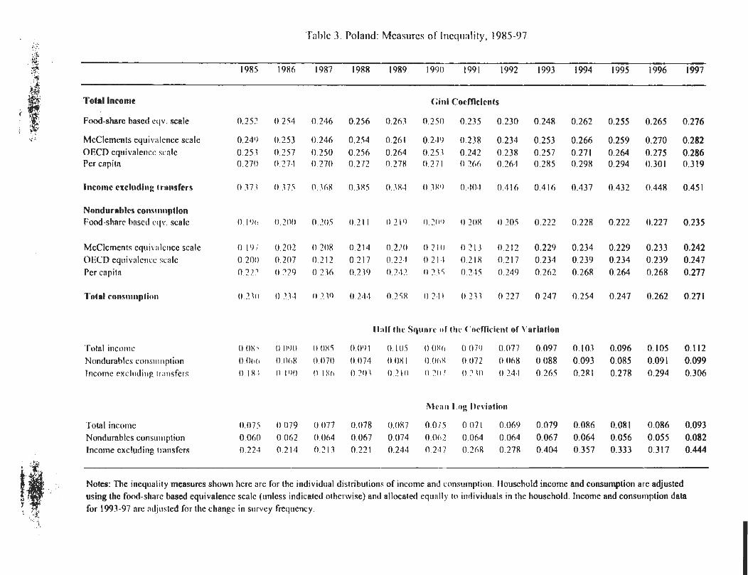
Table 3. Poland: Measures of Inequality, 1985-97

1985 1986 1987 1988 1989 1990

1991 1992 1993 1994 1995 1996 1997

Total Income Gini Coefficient s

Food-share based eqv. scale 0 .252 0 .254 0.246 0.256 0 .263 0 .250 0.235 0.230 0.248 0 .262 0 .255 0.265 0 .276

McClements equivalence scale 0 .249 (1 .253 0.246 0.254 0 .261 0 .219 0.238 0.234 0.253 0 .266 0.259 0.270 0 .282OECD equivalence scale 0.253 0 .257 0.250 0.256 0 .264 0 .253 0.242 0.238 0.257 0 .271 0 .264 0.275 0 .286Per capita 0 .270 0 .27 .1 0 270 0.272 0 .278 0 .271 0 266 0.264 0.285 0 .298 0.294 0.301 0 .319

Income excluding transfers 0 37I 0 .375 0.368 0.385 0 .384 (1 380 0.401 0 416 0 .416 0 .437 0.432 0 .448 0.45 1

Nondurables consumptio nFood-share based eqv . scale (1 . 196 0 . 2110 0 2115 0 .211 (1 . 219 0 209 0 208 II 205 0.222 0 .228 0 .222 0.227 0.23 5

McClements equivalence scale 0 .19 r 0 .202 (1 208 0 .214 0.220 0 210 0 213 0 .212 0.229 0 .234 0 .229 0.233 0 .242OECD equivalence scale 0 20(1 0 .21)7 0 212 0 217 0.221 0 21-1 0 .218 0 .217 0.234 0 .239 0.234 0.239 0 .24 7Per capita 0 .222 0 229 0 236 (1 . 239 0.242 0 215 0 215 0.249 0.262 0 .268 0 .264 0 .268 0 .27 7

Total consumption 0210 0 21-1 O 719 0 244 0 .258 0 2 . 11 (( .231 0 227 0 .247 0.254 0.247 0 .262 0.27 1

Total income (1 08' 11

(19(1 0 085 0 091

Half the Square of the Coefficient of Variation

0 .103 0 .096 0.105 0 .11 2O 105 0 080 O 019 O (177 0 .09 7

Nondurables consumption 0.066 0 1)68 0 117)) (( 1)74 0 .081 0 068 01)72 0 068 0.088 0 .093 0 .085 0.091 0.09 9Income excluding transfers 0 18 1 0

1 o o ) I t

1 8 6 0 201 0 . 2 1 1 1 O 207 0 210 0 .241 0 .265 0 .281 0 .278 0 .294 0.30 6

Total income 0.075 0 .079 0 077 0 .078 0 .087

Mean Log Deviation

0 .079 0.086 0.081 0 .086 0.09 30.075 0 .071 0 .06 9

Nondurables consumption 0.060 0 062 0 .1)64 0 .067 0 .074 0.062 0 .064 0 .064 0 .067 0.064 0.056 0 .055 0.08 2Income excluding transfers 0.224 0.214 0 .213 0 .221 0 .244 0.247 O 268 0 .278 0 .404 0.357 0.333 0.3I7 0.444

Notes : The inequality measures shown here are for the individual distributions of income and consumption . Household income and consumption are adjuste dusing the food-share based equivalence scale (unless indicated otherwise) and allocated equally to individuals in the household . Income and consumption data

for 1993-97 arc adjusted for the change in survey frequency .

1985

1986

1987

1988

1989

1990

1991

1992

1993

1994

1995

1996

199 7

Table4. Quantile Shares of Income and Consumptio n

Total Incom eQuantile range

< 20 9.0 9.l 9 . 5 9 .-1 9 . 3 9 .7 10 .4 10 .5 10 .2 9 .6 9 .9 9 .4 9 . l

21940 14 .8 14 .9 15 .0 147 4 .4 4 .9 153 5 .2 11 .6 14 .5 14 .6 11 .3 14 . 3

41-60 18 .5 18 .1 17 .9 17 .5 17 6 8 .0 184 8 6 17 .9 17 .9 17 .9 17 .7 17 . 8

61-80 23 .0 22 .4 22 0 21 .6 22 0 22 .3 22 .1 22 .8 22 .0 22 .0 22 .2 22 .0 22 . l

>80 34 .6 15 . 5 35 7 16 8 36 .7 35 .1 31 .1 12 . 9 35 .3 35 .9 35 .5 36 .6 16 . 8

< 20 2 .4 2 .2 2? 2' 2 .7

Income net of transfers

I .7 1 .2 l .3 0 .9 11 . 52 .2 1 .9 2 . 0

21-40 12 .7 12 .9 13 .3 12 .7 2 5 12 .5 12 .A 11 .3 112 10 .8 10 .7 10 .0 0 . 2

41-60 19 .0 18 .8 18 .7 (8 .0 18 .I 18 .6 189 18 .3 I7 .9 17 .8 17 .8 17 .3 17 . 7

61-80 25 .3 24 .4 24 .0 23 .1 24 .0 24 .8 25 .5 26 .0 24 .9 25 .1 25 .2 25 .l 25 . 1

>80 40.6 41 .6 41 .8 41 .1 42 .8 41 .8 41 .6 -12 .4 4-1.3 45 .2 45 .1 46 .7 .1 6 . 5

<20 10 .7 108 109 10 10I

Total consumption

07 III 11 .0 11 .l 10 .8 0 . 60 .6 I1 0

21-40 14 .6 14 .7 148 140 142 14 .7 150 14 .9 1510 149 14 .9 14 .7 4 . 8

41-60 18 .0 18 .0 178 170 76 180 182 18 .3 I8 .3 182 18 .3 18 .1 8 . 2

61-8(1 22 .4 22 .0 21 .8 21

8 22 .1 22 .1 22 .3 22 .5 22 3 22 3 22 .5 22 .5 22 . 5

80 34 .3 34 - 4 14 . 7 35 . 1 35 .9 14 .7 33 5 33 .6 313 33 .5 33 .2 33 .9 .1 . 9

<20 I1 .6 11 .7 11 .0 I1 .6 Il2

Nondurables consumption

1I

I ll .0 1I .1 I0 .8 10 . 611 .5 lI

8 11 . 2

21-40 15 .4 15 .7 15 .8 15 .5 15 .4 15 .6 (5 .8 15 .5 15 .0 I4 .9 14 .9 14 .7 14 . 8

4I-60 18 .7 18 .8 18 .7 18 .6 8 .6 18 .8 18 .7 18 .7 I8 .3 18 .2 18 .3 18 .1 8 . 2

61-80 22 .7 22 .4 22 .l 22 .3 22 .7 22 .5 2254 22 .6 22 .3 22 .3 22 .5 22 .5 22 . 5

>80 31 .7 31 .3 31 .5 32 .0 32 .2 31 .7 31 .3 32 .0 33 .3 33 .5 33 .2 33 .9 1 ; .9

Note : Each column indicates the share of aggregate income or consumption accounted for by persons within different quantile ranges for that variable .

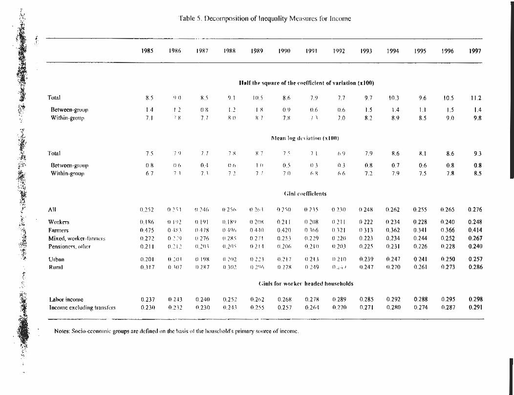
Table 6. Poverty Rates

incomeIncome excluding transfers:

lump-sum redistribution of transfersNondurablesconsumption

Year < 1/2 median < 2i3 median median < 213 median < 1/2 median < 2/3 median

1985 0 .03 0 .10 0 .10 0 .17 0 .01 0.051986 0 .03 0d0 0 .09 0 .16 0 .01 0.061987 0 .04 0.11 0 .I0 0 .17 0 .01 0.081988 0 .03 0 .08 9 9 .09 0 .15 0 .01 0 .071989 0 .02 0 .07 0 .08

0.100 .01 0 .07

1990 0 .06 0 .20 0 .13 025 0 .04 0 .1 71991 0 .05 0 .1 7 0 .13 0 .20 0 .04 0 .161992 0 .06 0 .20 0 .16 0 .27 0 .04 0 .1 8

1993 0 .08 0 .23 1) .16 0 .29 0 .00 0 .171994 0 .10 =b ') .18 0 .31 0 .06 0 .2 31995 0 .09 x ) .2 .1 0.17 0.30 0 .06 0 .22:996 0 .08 2 : 1- 0 .28 0 .05 0 .20

1997 0 .07 18 0 .I5 0 .25 0 .05 0 .19

Notes : Household income and consumption are adjusted by food-share based equivalence scales and deflated by theaggregate CPI . Each individual in a

en household is then assigned the same level of income or consumption .The poverty lines based on median real income and real consumption are computed using data across all years . Eachcolumn indicates the fraction of the sample population below 1.2 or 2 .3 of median real income or consumption ,

respectively . Median annual real income and real nondurables consumption at 1992:Q4 prices are, respectively ,

3,370 and 2,829 in new zloty (I0 .000 old zloty = 1 new zloty) . Using the OECD PPP exchange rate for 19920 .677 new zloty = US$1) . this yields income poverty lines expressed in U .S . dollars of 2 .192 (1 .2 median) and

3 .323 (2,3 median) per equivalent unit . The corresponding poverty lines based on consumption are 2,089 and 2,786 .Poverty lines for different families can be constructed using the equivalence scales in the last column of Table B1 .

The poverty lines are the same for the first and second panels .

Table 7. Social Transfers

1988

1989

1990

1991

1992

1993

1994

1995

1996

1997

General Government Expenditures(in percent ofGDP )Cash transfers to individuals

9 .4

11 .2

I0.6

17 .3

19.9

20 .-1

20.2

19 .7

18 .7

19 . 4

Pensions

7 . I

8 .2

8 I

12 .2

11 .8

15 .0

14 .9

14 .5

14 .3

14 . 4

Unemployment benefits

0 0

(l O

I1 2

1 2

l .7

l .2

I .2

1 .2

1 .1

1 . 0

Other benefits

2 .3

3 .0

2 3

3 .9

3 .4

4 .2

4 . I

4 .0

3 .3

4 . 0

Mean Cash Transfers (HBS data)

Total transfers

41 154

41792

3625 , 1

449 , 18

44691

43486

44171

44860

46786

48197

(avg . ratio to total income)

(23 .4)

(21 .8)

(26 .3)

(32 .2)

(33 .6)

(31 .6)

(32.8)

(32.7)

(32 .4)

(31 .3)

Pensions

29857

30, 197

273117

33520

333,16

33172

34672

36240

38008

4071 5

(avg. ratio to total income)

(17 .0)

(15 .9)

(19 .8)

(24 .0)

(25 .l)

(24 .l)

(25 .8)

(26 .4)

(26 .3)

(26.4)

Other cash benefits (incl . Ul)

11280

11279

8927

11404

1 1323

10315

9498

8620

8777

7482

(avg. ratio to total income)

(6 1)

(5 .9)

(6 5)

(8 .2)

(8 5)

(7 .5)

(7 .l)

(6 .3)

(6 .1)

(4 .9)

general Government Balance(in percent of GDP)

0 .0

-7 .4

3 .l

-6 .5

-6 .7

-2 .9

-3 .0

-3 .1

-3,4

-3 . 1

Seal GDP (annual % change)

4 .0

0 .3

-1 1 .6

-7 .0

2 .6

3 .8

5 .2

7 .0

6 .1

6 .9

Notes : The data on real GDP and government expenditures are taken from various IMF sources . The figures in the middle panel (mean

transfers in HBS data) are expressed in terms of 199204 prices.

Table 8. Cross-Country Dat a

Annualized Gini coefficients Average cash Initia lcumulative transfers Transition condition

Country GDP growth Pre-transition Post-transitionDifference

(% of (GDP) indicators indicato r

Poland l .25 0 272 0 301 II 029 7 .7 14 .3 1 .1 8Slovenia 0.47 0

17 . 1 0 .22 1 1) 049 14-8 13 .0 1 .2 4Czech Republic -0 .29 0 194 0 .25 1 0 .061) 12 .l 14 .7 1 .4 3Slovak Republic -0 .56 0 195 . . 11 .8 13 .3 1 .2 5Hungary -l .15 0 .248 0 .308 0 060 6 .5 14 .7 1 .4 7Uzbekistan -2 .17 0 282 . . 11 .5 9 .0 -l .1 5Romania -2 .18 0 .233 0 280 0 .047 8 .9 9 .8 0 .9 4Estonia -3 .05 0 230 0 .351 11 .124 l(1 .0 12 .5 -0 .3 3Belarus -4 .23 O 228 0 .28X 0 .060 8 .9 8 .3 -1 .1 9Kazakhstan -5 .03 0 257 0 .35-1 (1 .097 6 .9 8 .3 -1 .0 7Bulgaria -5 .03 0 228 0 317 0 .089 11 .8 10 .3 0 .5 5Lithuania -5 .65 0 225 0 32-1 0 .099 9 . 6 I0 .5 -0 .5 2Russia -6 .14 0 218 0 .3811 11 .142 7 .5 9 .7 -0 .3 4Kyrgyzstan -6 .67 1) 260 0.40 5 11 .145 12 .4 10 .3 -l .0 3Latvia -6 .89 0 225 0 . 1')t 0 . 095 11 .8 10 .2 -0 .4 6Turkmenistan -10 .27 0 26-1 3 .l 4 .3 -1 .2 7

Ukraine -10 .64 (( 231 017 t 1) 2 . 10 9 .4 8 .7 -0 .9 1Moldova -10 .89 (I 241 9 4 9 .7 -0 .80

Notes : Annualized cumulative GDP growth is measured over the first eight cars of transition . "l he first year of transition is 1990 for Bulgaria, the Czec h

Republic, Hungary, Poland, Romania, and the Slovak Republic ; 1991 for Slovenia ; and 1992 for the Baltics, Russia and other countries of the former Sovie tUnion. Data on Gini coefficients were taken from Milanovic (1998, 1999), World Bank (1997, 1999, 2000), OECD (1997) and, for Poland, from this paperData on average cash transfers from the transition years through 1997 arc from Milanovic (1998) . The transition indicator is a weighted average of th etransition indicators in the EBRD's 1995 Transition Report (Table 2 .l) . The index of the difficulty of initial conditions (a higher score indicates mor efavorable conditions) is taken from de Melo, Denizer, Gelb, and Tenev (1997 )

Table 9 . Cross-Country Regressions

Dependent variable: Annualized cumulative real GDP growth in first 8 years of transition

( 1) (2) (3) (1,4) (5) (6)

Change in Gini *100 -0.520* . . . . . . -0.365' -0 .381* -0.442*

(0 .089) (0.075) (0 .065) (0.149)

Transition indicator . . 1 .121* . . 0 .587* 0.671* 0.599*0 .261) j 0 .243) ( 0 .154) (0.225)

Initial conditions index . . . 2 .617* 0 .283 . . . . . .

(0 .562) (0.616 )

Constant 1 .020 -16.388* -1.124* -6.990* -7.757* -6 .373

(0 .967) (2.952) (0.551) (2 .751) 2.107) (3 .731)

Adjusted Rsquared -2 0 .57 0 .61 0 .83 0 .89 0 .88

Number of observations 14 14 14 i 4 14 14

Notes: A positive change in the Gini coefficient reflects an increase m inequality after the transition . The

transition indicator captures progress in various dimensions of transition to a market economy. A higher

value indicates better progress . The initial conditions index is defined such that a higher value indicates .

:more favorable initial conditions at the start of transition . See Table 8 for a detaile d description

of the data used in these regressions . Regressions (l) throu gh (5) are OLS specifications . while regression

(6) is an IV specification with the initial conditions index used as an instrument for the change in the Gin i

coefficient. Standard errors are reported in parentheses . An asterisk indicates statistical significance a t

the 5 percent level .

Table Al . Regressions Using Income Residual s

Workers Farmers Workers/farmers Pensioners

Time O .001 0.006 O .006 0.000

(0.002) (0 .006) (0.006) (0.001 )

Time ^2/10^3 O .000 O.188 -0.171 -0.002

(O.000) (0 .092) (0.092) (0.023)

Time ^3/10^6 0.001 O.919 0 .859 -0.009

(0 .010) (0 .365) (0.364) (0 .095)

Mean real income 0 .207 O.126 0 .116 0.367

+O .014) (0.013) (0.021) (0 .027)

Dummy for 93-97 ) .16~ ')369 ') .201 O .044

(O .028) (0.102) (O.098) (0.026)

Adjusted Rsquared O .88 O .65 0 .51 0.85

Number of observations 92 92 92 92

Notes: The dependent variable is the log standard deviation of the residuals fro m

equation (l) . Standard errors are reported in parentheses .

Table B l . Equivalence Scales as a Function of Household Compositio n

Food-Share Equation s

Household Type :GUS

(OECD McClements OLS I V

Single person households

1 HD = Male, 31-60 0.54 0 .59 0 .55 0 .74 0 .7 1

2 HD = Male, 18-30 0 .50 0 .59 0.55 0.72 0 .70

3 HD = Male. >60 0.50 0 .59 0 .55 0 .74 0 .68

4 HD = Female, 3I-60 0 .06 0 .59 0 .55 0 .66 0 .6 5

5HD = Female, I8-30 ? . 16 0 .59 0 .55 0 .63 0 .646HD = Female . >60 to 0 .59 0 .55 0 .60 0 .5 3

Married Couples

00 1 .00 1 .00 1 .00 I .00HD = Male . 31-60 : Female. 31 -60)

8

HD = Male, 18-30 : Female 18-30 00 1 .00 0 .91 0 .9 2

9

HD = Male . >60 : Female 060 00 ; .00 1 .00 1 .03 0 .9 2

Married couples with one ki dHD = Male . 31-60 : Female . 31-60

29 11 .12 1 .I 01')

Male/Female, < 7

1 1 Male/Female, 8-12 .32 1 .29 1 .20 1 .16 1d 4

2

Male, 13-17 46 29 . .19 1 .1 7

:3

Female, 13-I7 ~l 29 1 .29 1 .10 I .1 3

Married Couples with older dependent sHD = Male, 31-60 ; Female, 3I-60

1 .50 :

01 :00 1 .20 I .2 314 Male . >60

15

Female, >60 1 .06 1 .01 1 .40 1 .32 1 .29

16

Male . >60: Female. >60 2 .00 2 .00 1 .80 1 .63 I .59

Notes : HD indicates the head of household . The equiva ł ence scales shown in the last two columns are based on OLS

and IV estimates, respectively, of food share equations using the HBS data. Equivalence scales based on IV estimates(column 5) are used in the paper.

Figure 1 . Income and Consumption Quantile Ratios

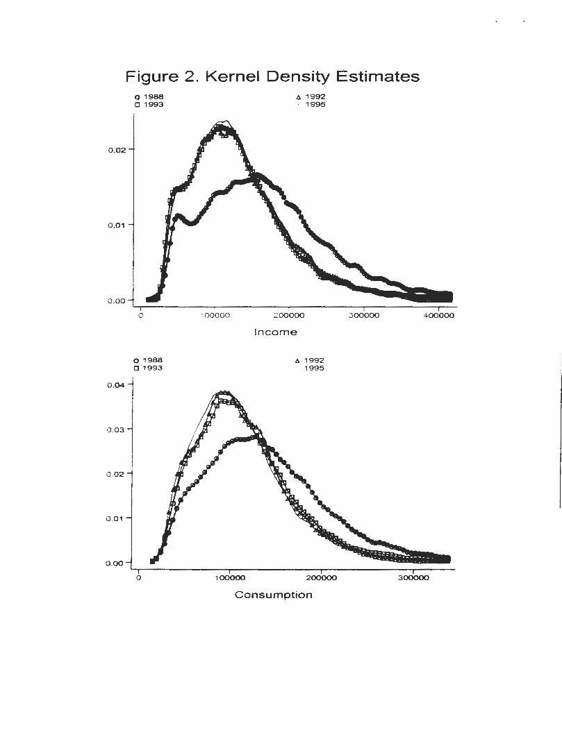
Figure 2 . Kernel Density Estimates

Figure 3 . Kernel Density Estimates : Adj . Income

Figure 4 . Median income, consumption for diff . socioeconomic groups

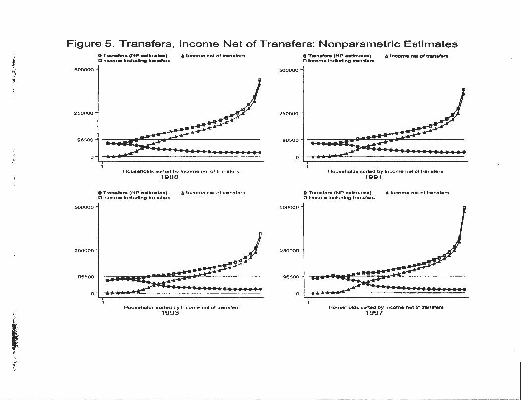
Figure 5 . Transfers, Income Net of Transfers : Nonparametric Estimates

Figure 6 . Transfers, Inequality and Growth During Transition

Figure Al . Income Residuals, Fitted Values from Stage II Regressions

Figure A2 . Time Polynomials, Stage II Regression s

Fitted Time Polynomials + Estimated Dummy for 93-97