inequality: is it a result of globalization?

ICADE BUSINESS SCHOOL

INEQUALITY: IS IT A RESULT OF GLOBALIZATION?

Autor: Marta Aldasoro Frías

Director: Santiago Budría Rodriguez

MadridJunio de 2017

1

Marta Aldasoro

Frías

INEQ

UA

LITY

: IS

IT A

RES

ULT

OF

GLO

BA

LIZA

TIO

N?

2

Abstrac t This paper reviews the trends for the period 1980-2015 of some of the main macroeconomic variables of the countries of

greater interest of our sample and investigates the determinants influencing the variance of the Gini coefficients as representative of inequality measurement. The empirical results observed when comparing the results of the regression modelling obtained one clear conclusion can be drawn: the two determinants that are significant for all three country groups are Population and Globalization. Population has a positive effect in increasing inequality of income distribution for all of them, whereas globalization has only a positive effect in European countries and emerging countries, but with a big impact over the same, but in the United States in has a negative effect, reducing inequality levels of income distribution. The question regarding the decisions of the UK and the USA of adopting protectionist measures, and if it is a good idea is answer it terms of globalization and income distribution inequality finding that it would be a positive decision for the UK and a negative one for USA. Key words: Globalization, Technological progress, Inequality, and International Trade.

3

INDEX ABSTRACT 2

INTRODUCTION 4

OBJECTIVES 6

RELATED INVESTIGATIONS 7

CAPITAL IN THE TWENTY-FIRST CENTURY 7 EMPIRICAL ANALYSIS ON THE DETERMINANTS OF INCOME INEQUALITY IN KOREA 10

THEORETICAL FRAME 11

GROSS DOMESTIC PRODUCT (GDP) 11 GROSS DOMESTIC PRODUCT PER CAPITA (GDPPC) 13 EVOLUTION OF POPULATION 15 EXPORTS AND IMPORTS 15 GINI INDEX 17 UNEMPLOYMENT 18 INFLATION 19

METHODOLOGY 20

TIME SERIES 20 OBJECTIVES OF TIME SERIES ANALYSIS 20 COMPONENTS OF A TIME SERIES 21 DESCRIPTIVE ANALYSIS OF TIME SERIES 21 CLASSIFICATION OF TIME SERIES 22 TREND ESTIMATION 22 POSSIBLE ESTIMATION PROBLEMS: SEASONALITY OF DATA 23 PANEL DATA 26 OBJECTIVES OF PANEL DATA ANALYSIS 26 SPECIFICATION OF A PANEL DATA MODEL 26 ADVANTAGES AND DISADVANTAGES OF THE PANEL DATA TECHNIQUE 27

DATA ANALYSIS 28

EUROPEAN COUNTRIES DESCRIPTIVE STATISTICS 29 UNITED STATES DESCRIPTIVE STATISTICS 29 EMERGING COUNTRIES DESCRIPTIVE STATISTICS 29

ANALYSIS OF RESULTS 30

EUROPEAN COUNTRIES 30 UNITED STATES 31 EMERGING COUNTRIES 31 COMPARISON OF COEFFICIENTS OF DETERMINANT VARIABLES BETWEEN COUNTRIES 32 LIMITATIONS OF OUR PROPOSED MODEL 33

CONCLUSIONS 34

REFERENCES 35

BOOKS 35 REPORTS 38 ARTICLES 38 INTERNET WEBPAGES 38

ANNEX 38

VARIABLES USED IN THE REGRESSION 39

4

INTRODUCTION

“The idea of comparative advantage—with its implication that trade between two nations normally raises the real incomes of both—is, like evolution via natural selection, a concept that seems simple and compelling to those who understand it. Yet anyone who becomes involved in discussions of international trade beyond the narrow circle of academic economists quickly realizes that it must be, in some sense, a very difficult

concept indeed.”

Paul Krugman y Maurice Obstfeld1

Globalization is the process by which countries or nations open their barriers to exchange capital, goods

and services, etc. The International Monetary Fund defines it as follows, “Globalization refers to the increasing integration of economies around the world, particularly through the movement of goods, services, and capital across borders”2. However, it is a very controversial issue, as it will be seen, and a very popular topic nowadays.

The present times raise a huge interest in the possible consequences of both the Brexit and the

protectionist policies the United States of America is undertaking. Many economists give their opinion on this matter, and many agree that not only can there be consequences on the economy, but also on the general welfare of the population.

Over the years, economists have considered free trade as a vehicle to increase total income or welfare of countries as well as their productivity, essentially with a positive focus on exports, which create employment, and negative on imports, which destroy it. Moreover, the theory of endogenous growth tells us that in the case of talking about a small country, this country will not be able to live outside international trade, so we observe a dependence of the modern economy on this activity or a co-dependency between countries.

The problem is that globalization, due to the difficulty to find the correct balance of international trade, is not only a source of income, but also of inequality. This phenomenon is increasingly being studied as a matter of worrisome, as for instance by Professor Elhanan Helpman. Helpman is a professor at Harvard University and is a scholar specialized in economic growth and international trade. This economist argues that the growing inequality that we have been seeing these past years is not created by factors such as the loss of influence suffered by unions or the fall in real terms of minimum wages, but the two following factors: international trade and change or technological advance.

On the one hand, with respect to international trade, developed countries follow a similar trend with

respect to their preferences: they import products that are low-skilled labour-intensive and export high-skilled labour-intensive products. This implies a rise in the demand for skilled workers by companies in industrialized countries, which has a positive effect on the salary of this group with respect to workers with a low qualification, which causes an increase of the wage gap between these two groups, or what is equal to a greater inequality.

Technological progress has also been argued to have the same effect as international trade. With a greater use and advance of technology, it is also necessary for workers to have knowledge of how to use this technology, as it is implemented in all sectors. Therefore, with the advance and implementation of technology, the demand for skilled workers, or technology savvy individuals, is also increasing, and thus the salary is also increased with respect to low-skilled workers and, once again, increasing the wage gap between these two groups.

The technological progress lived in the past decades is unique in the history of mankind. There have

never been so many discoveries in such a short period of time in both technological and scientific fields. Capitalism and globalization are participants of the huge technological advance due to the creation of greater synergies as result of the global acquaintanceship of today´s economies.

1 Krugman, Paul R. And Maurice Obstfeld, The Economics and Politics of International Trade: Freedom and Trade, Volume II, page 22 2 https://globalisms.wordpress.com/imfs-definition/ - International Monetary Fund

5

Elhanan Helpman gets to the conclusion in his papers that international trade effectively contributes in great amount to the increase of inequality, but it is the technological advance that has most weight in this wage difference.

The statements of this economist are corroborated by the report of the International Monetary Fund (IMF) "World Economic Outlook"3 released this past April of 2017. This report asserts that globalization is necessary for international prosperity because, not only increases the productivity and growth of a country as mentioned above, but also facilitate the access to capital and technology, and this increases welfare and reduces poverty.

The report quantifies the effect of globalization and technology on which Helpman's work is based, with

technology being the most explanatory variable of the decline in wages, accounting for 50% of this decline and globalization accounting for 25%, reaching the lowest registered wage level for half a century.

Globalization and technology are having the same effect on the income distribution mentioned by

Helpman since, given the shift in activity from production to more capital-focused activities, demand for skilled workers rises with respect to unskilled workers, and this is increasing global inequality. The concern of the IMF is that the impact of these advances in technology and globalization is greater on the wages of the second group mentioned, and not so much on the first, asking countries to strive to take measures for the distribution of income in a more equitable way, in order to reduce these social effects derived from technology and globalization. After the opening of the Chinese economy in the 1980´s, China has not yet encountered a mechanism to ensure a reduction of its inequality levels. The economic theory asserts the fact that poverty and inequality are inefficient in a market economy. However, the high levels of economic growth experienced by China in the last decade resulted in a greater income distribution and hence, declining poverty. Although, according to Dwayne Benjamin, the reforms have drastically increased China´s inequality. He assures that the rapid economic growth has led to a significant reduction of poverty in rural areas whereas it has only virtually eliminated poverty in urban areas, and all this should be contrasted with the increase of economic inequalities. The United States of America is nowadays known as the most inegalitarian developed country on Earth. Thomas Piketty, Emanuel Saez and Gabriel Zucman, outstanding global inequality experts have developed studies were it is observable that the past four decades have showed the fastest redistribution effect of income towards the rich people of the entire history. These authors also talk about the abrupt change of trend there was between periods, being the first the period from 1946 to 1980 and the second from 1980 to the present. One of the reasons the authors give for the widening of this income gap is the stock market and the benefits got from capital. The upper class has benefited from speculative bubbles, transferring with these actions colossal amounts of money. Historians often remember that before the emergence of monopolies and financial capital, the American economy was the most socially egalitarian of the Western world, but since the latter part of the nineteenth century the United States has transformed into a country of “capitalist thieves”. In India, the problem of inequality may be due to several reasons. There is a religious issue that divides the society between castes or classes that determines from its future labor until the person with whom they can marry. But analysts say that globalization is a factor that helps to intensify this inequality. India is becoming a power in open digital economy. This requires a higher educational level of society, but given the great inequality of society and its distribution by caste that is not an option for a large part of the population. Therefore, globalization could effectively contribute to the increase in inequality in India. Until 1980 the United Kingdom had remained as a country with really low wealth inequality, but due to the second globalization wave the distribution of wealth in this country changed dramatically. This is shown very clearly in the latest report of Alvaredo, Atkinson and Morelli were they clarify the following: “The UK went from being more unequal in terms of wealth than the US to being less unequal. However, the decline in UK wealth concentration came to an end around 1980, and since then there is evidence of an increase in top shares, notably in the distribution of wealth

3 http://www.imf.org/en/Publications/WEO/Issues/2017/04/04/world-economic-outlook-april-2017

6

excluding housing in recent years”.4 Nowadays, the UK is one of the developed countries with a greatest wealth gap. The 1% richest part of UK´s population is 20 times wealthier than the 20% part of the population with least resources, according to this report. Moreover, the five richest families are wealthier than 12 million British citizens. In its last report Oxfam classifies Spain as the second country of the European Union with the greatest inequality growth since the burst of the Great Recession. This country has been experiencing an economic recovery shown by the growth of its GDP since 2014, but this growth has not been reflected in the incomes of the population with the lowest level of rent. As the OCDE and INE data show, in 2015 the poorest segment of the population lost 33.4% of their wealth, whilst the three richest people of the country saw their wealth increase by 3%. The wealth of these three people quantifies as the same as the 30% of the poorest population of the country. It is observable the importance of the wealth gap of this country. To carry out this end of master project, previous theories and analysis of reliable sources on this matter, as well as using databases of international organizations as a data recollection resource will be used as motivation, being the main references in this aspect the International Monetary Fund, the World Bank and the OECD data webpages amongst others.

OBJECTIVES

The objective of this end of master Project is to effectively quantify the variables which have increased inequality during the years, to see if the United Kingdom and the United States of America are following the correct path into a level of international trade which reduces the inequality in their countries, or if this situation will only worsen the allocation of income, causing more poverty and inequalities.

The is an aim to address if in fact globalization has been a significant variable in order to increase

inequality, or if other variables are more significant to see if effectively the United Kingdom and the United States of America are taking the right decision when opting for protectionist policies or measures. The UK and the USA are the highlighted countries because of their recent decisions towards protectionism, to observe the possible effects. This matter is important as there could be a contagion effect within countries as for example the case of France with Marie Le Pain, or the tense situation with the European Union, as people every day are more and more worried about the future of their economies due to the current situation.

This paper will start by talking about previous investigations documenting about this issue. The book

“Capital in the Twenty-First Century” by Thomas Piketty will be useful in order to get a first image about some of the countries we will be investigating. In this section it will be shown the evolution of inequality documented by this author and the evolution of the 1% richest population of the US, the comparison between US´s and European Union´s wealth and taking also a look at the information recollected about emerging countries.

In the second section of this paper some theoretical information and definition of relevant variables will

be provided in order to fully understand the variables that will be studied and presented along this paper. Followed by doing a brief overview of the current information about this issue, doing a comparison of some relevant variables for the countries to analyse. It will be a contrast between developed and emerging countries, which could be relevant in order to determine the importance of factors as globalization or technological advance due to their different stages of development and commercial opening. An analysis of countries or union of countries will be carried out, in economic and political aspects which are developed, as for example countries of Europe as Spain and the United Kingdom or the United States of America, comparing it to countries as China and India, which are developing at a really fast pace in the last years, and could be very illustrative for this study.

After the methodology that will be used will be explained, and the variables of the econometric model that will be used in order to explain the main variable: inequality, as well as trying to do a forecast about the future of some countries. The econometric methodology to be used will be a time series analysis, which will be

4 Alvaredo, Facundo, Atkinson, Anthony B. and Morelli, Salvatore, Top Wealth Shares in the UK over more than a Century, WID.world working paper series nº 2017/2

7

helpful for doing a descriptive analysis in the first instance, helping us to understand the data in more depth. Some examples of graph analysis and visually detecting seasonality and trend will be provided, as well as explaining the main problems the model can have and the way of taking out these factors.

Once the study has been carried out, a descriptive analysis of the data, as well as an explanation of the

variables used, how they were obtained or created in some cases will be exposed. The estimation of the regression will give a series of values for the betas of each of the variables that are believed to be a determinant of the distribution of the income inequality that will be used as comparison between countries.

Finally there would be exposed the conclusions of the investigation.

RELATED INVESTIGATIONS

The inequality debate and its possible causes is a very in the mainstream topic. There are plenty of scholars investigating the reasons or factors that are causing the increase of inequality worldwide. Between them, we can mention Thomas Piketty, a French economist and author of the book “Capital in the Twenty-First Century”, which talks about income and wealth inequality looking at historical data and evolution in the last century.

Generally, when it comes to quantifying the variables and the impact they have on inequality increase,

the most used variable to represent inequality is the Gini Coefficient. The report “Empirical Analysis on the Determinants of Income Inequality in Korea” is an example of a report using this variable. This paper published in the International Journal of Advanced Science and Technology and written by Hae-Young Lee, Jongsung Kim and Beom Cheol Cin, will be a motivation for the variables selection of this study, as its aim it to determine the variables affecting the income inequality in Korea. In this study the same will be done for the selected country sample.

Capital in the Twenty-Firs t Century Although this book talks in great part of the situation of France, it also talks about other countries that

result interesting for our study, as for example the US or China amongst others. He and his colleagues make use of simple variables and easy to understand chart illustrations. “Piketty and his colleagues have deployed their charts to reshape the entire inequality debate”- The New Yorker.

In the following graph Piketty analyses the income inequality in the US since 1910. It is observable a U

shape that we will see in the analysis of inequality of other countries which is representative of a situation of high inequality, followed by an intense decrease of inequality during a prolonged period of time and the successive increase of inequality. It could be due to the stock market crash of 1929 very well known as the “Black Thursday”. The crash of the stock market decreases the wealth of the population with higher living standards, that as it is also seen in this book, usually have great part of their returns in financial products, and therefore it decreases the inequality.

Graph 1.1: Income Inequality in the United States

8

Source: piketty.pse.ens.fr/capital21c5 The fact that many rich people tend to invest their money in financial instruments and this could be the

reason for the inequality levels from the past due to the Black Thursday could be verified in the following graph. In this graph he analyses the income and wealth of various groups. In the past years it is very common the analysis of the income or wealth of the median or middle class population, but there were not many investigations about the so called “top one per cent” and this author does consider this population “elite”. This is observed in the following chart.

Graph 1.2: Decomposition of US´s top income decile

Source: piketty.pse.ens.fr/capital21c6

In this graph the U shape mentioned above for the top 1%, 5% and 10% annual incomes is once again

observable. Comparing this graph to the previous one it can see that this group’s trend follows the total inequality in the US, which could mean it is the principal cause of it. The other two categories in this graph follow a much more stable evolution in an upward trend since 1940. For all three groups it is seen that in the Great Recession their income falls, or slows down at least, but soon they recover. It is the top 1% which represents the greatest part of inequality, being observable that it has a great increase of their income going from a 10% share of national income in 1980 to doubling it to a 20%in 2010.

In the following chart the author introduces data from Europe, and compares it to the US levels. As he

clarifies in the text, although Europe had had during great part of the history greater levels of inequality, this changes decades ago for the US to become the country with the highest inequality levels.

Graph 1.3: Wealth inequality in Europe vs. US

5 Thomas Piketty, Capital in the Twenty-First Century, page 32 6 Thomas Piketty, Capital in the Twenty-First Century, page 297

9

Source: piketty.pse.ens.fr/capital21c7 This graph does not talk about income, but about wealth. It is a comparison between the historical levels

of wealth inequality of the top 10% and top 1% of United stated and Europe. During the period being observed it is appreciated that Europe has a wealth distribution more unequal than the US. It is in 1960 when this trend changes, and reverts, becoming the US more wealthy unequal than Europe, and this levels have maintained ever since.

Forbes Magazine releases every year a list of the top 10 wealthiest people in the world. In 2010 three of these where from the United States: Bill Gates with 53,000 million dollars, Warren Buffet with 47,000 million dollars and Lawrence Ellison with 28,000 million dollars, which is a total of 128,000 million dollars being owned by only three individuals in the US. There were also three men in this list from Europe, Amancio Ortega, Bernard Arnault and Karl Albrecht, owning between the three of them 76,000 million dollars which, although being immensely high, 52,000 million dollars less that what is owned by the US individuals mentioned before. With this an assertion is not being done about if this people are the main factor of the wealth inequality distribution of course but they do affect upwards when doing a mean, as the mean takes into account these incomes.

Not only he does a comparison with Europe but Piketty also realizes a comparison with emerging countries as we observe in the following chart and which results of great interest for this study:

Graph 1.4: Income Inequality in emerging countries


7Thomas Piketty, Capital in the Twenty-First Century, page 3558 Thomas Piketty, Capital in the Twenty-First Century, page 333

10

The famous U shape is once again observed for emerging or developing countries. Looking at the top percentage of inequality reached by this countries, and comparing them to United States levels we can conclude that the US still has much higher inequality levels than emerging countries overall. Although, it is observable than countries as Colombia, Argentina or South Africa is highly income inequitative. It is interesting to observe China´s inequality levels. Although China has been growing exponentially, the inequality has also increased immensely.

Finally there is a graph that illustrates Piketty´s investigation conclusions. The graph illustrates the rate

of return of capital after taxes and capital losses comparing it to the worldwide output growth. The rate of return of capital was higher than the growth rate for great part of history, but after World War II until nowadays this exceptionally changed, being the output growth higher than the rate of return of capital, but Piketty believes there are signs showing this is coming to an end, and it will if the tax rate of return on capital continues to be 30%. In the following graph it is also observable the author´s estimates about the future situation.

Graph 1.5: Rate of return of capital versus growth rate of world output


Piketty concludes that there is a “central contradiction” with the theory of capitalism. Growth rate has normally been below the rate of return, which is translated into a steady rising inequality, but “the consequences for the long-term dynamics of the wealth distribution are potentially terrifying”10. When r > g it is a sign that the wealth created in the past grows at a higher pace than the world output and wages, creating a great inequality in society. His solution to this issue is to apply a progressive tax on capital returns, “This will make it possible to avoid an endless inegalitarian spiral while preserving competition and incentives for new instances of primitive accumulation… This would contain the unlimited growth of global inequality of wealth, which is currently increasing at a rate that cannot be sustained in the long run”11

The difficulty to this thought, as Piketty says, is the necessity of international cooperation also with respect to policy application to achieve an efficacious regulation on capitalism. With the nowadays situation were instead of integrating countries it seems there is an increasing tendency to disharmonize the possibility suggested by this author of integrating policies seems fairly improbable.

Empiri cal Analys is on the Determinants o f Income Inequal i ty in Korea This paper observes the trends of income inequality in Korea in the time period 1980-2012. Furthermore, this paper tries to find the determinants influencing this income distribution inequality, and will be a motivation source in order to choose the variables in the actual study. The variables used in the Korean Empirical analysis are the following:

Description Definition Nominal GDP per capita (in Won) Ln (GDP/population)

9 Thomas Piketty, Capital in the Twenty-First Century, page 362 10 Thomas Piketty, Capital in the Twenty-First Century, page 577 11 Thomas Piketty, Capital in the Twenty-First Century, page 578

11

Yearly consumer price growth rate %Variation CPI Share of elderly population Population over 65/working-age population Share of middle school students Middle school students/school-aged population Growth rate of agricultural product % Variation in agricultural production Unemployment rate Unemployed/working-age population Female employment rate Female employment/working-age population Share of self employed Self-employed/employed Foreign direct investment Ln (FDI) Trade openness (Exports + Imports)/GNI Share of import Imports/GNI Share of investment Investment/GDP Share of government spending Government spending/GNI

Source: own creation taken from the report12 What the study reveals is that Korea´s inequality increases from 2003 to 2009, when it reaches a peak, and then it starts to decrease in 2010, maintaining a constant level since 2011. The decile ratio for households for both market income and disposable income increased until 2011, being a relevant factor in the increase of the Gini Index. On the other hand, the variable of government spending as a share of GNI was found not to be relevant in the increase of inequality in Korea. The investment share in GDP shows a negative correlation with the income distribution, in other words, as the investment share of GDP increases, the distribution inequality decreases. Another variable that presents a negative estimate over inequality is the level of education or share of middle school students in school-age population As a factor found to increase income inequality it was revealed to be the share for the elderly in working population. Korea´s population has been having aging problems, just like Spain, and it was found to be one of the variables that most influences the increase of income distribution inequality. Finally, the share of trade volume, or what could also be called globalization, showed a positive, significant estimate, meaning that as the trade volume over GNI increases, income inequality increases.

A remarkable sentence in this paper is “As Stockhammer (2010) argues, three major building blocks of neo-liberalism – globalization, financialization and rising inequality – are closely intertwined to create the imbalances that caused the most recent global economic crisis.” At the end of this paper it will be confirmed if this sentence applies to the research that will be carried out in this study.

THEORETICAL FRAME The previous studies served as motivation to try and quantify the several shocks or factors affecting the

level of inequality of the society, that also have to be considered in this study to see what is the real weight globalization is having over the increase of social divergence.

Gross Domest i c Product (GDP) Gross Domestic Product, GDP from now on, is the value given to the final goods and services produced in

a country during a determined period of time. It is the most used indicator to measure the economic dimensions of the countries. It is composed by the following variables;

- Consumption (C): the goods and services purchased by consumers. It is the largest component of GDP.

- Investment (I): the sum of non-residential investment, which is the purchase of new plants or machines by companies, and residential investment, which is the purchase of new housing by individuals.

- Public Spending (G): goods and services purchased by the State in all its instances.

12 Lee, Kim and Cin (2013), Empirical Analysis on the Determinants of Income Inequality in Korea, page 101

12

- Exports (X): purchases of domestic goods and services by foreigners.

- Imports (I): purchases of foreign goods and services by consumers, businesses and the State.

To this GDP variables mentioned, there are others that are interconnected, and affect in great measure to the last ones:

- Inflation: it is a continuous rise of the general price level of the economy.

- Inflation rate: rate at which this price level rises.

- Unemployment rate: coefficient between the number of the people unemployed and the active population. High unemployment rate indicates that the economy may not be using some of its resources efficiently; therefore the economy does not work correctly.

o Active population = employed + unemployed

o Unemployed: is the number of people without work but who are looking for one. It is important to make this specification because there are people that have stopped looking and they must not be included in this group.

These last variables will also be studied in this paper for the countries of our interest.

To start off the GDP for China, the United Stated, the European Union, United Kingdom, Spain, the OECD members, India and the World data have been graphed for the period 1960 to 2014, and measured in current US dollars. With this graph it can be seen in absolute terms the comparison between developed and emerging countries.

Graph 2. 1: Gross domestic Product (GDP) current US dollars

Source: Own creation with data from Worldbank13

It is said that there have been two globalization waves, the first around 1960 and a second one around

1980. In the graph it is appreciable that from 1960 United States and Europe grew exponentially being part of the first globalization wave. United States grew in a more stable way, whereas Europe has more peaks and lows but having always the United States as a reference line where it seems to always come back.

On the other hand, China and India do not follow the same trend as the last mentioned. China

maintains a really low and stable GDP until 1980 when it takes advantage of the second globalization wave and starts to grow slowly and in 2000 when it starts growing exponentially. China offers preferential fiscal advantages

13 http://data.worldbank.org/indicator/NY.GDP.MKTP.CD

13

to foreign investors, which has made China the greatest enterprise receptor in a worldwide level, which is one of the reasons that explain the GDP growth experienced by this country in the last decades.

India also took advantage of the second globalization wave, but has not grown with the same intensity as

China, although it has seen its GDP grow considerably. In 2000 its GDP grows at a further pace, following China´s trend, although in a lower magnitude.

United Kingdom and Spain also see a substantial growth in their GDP since 1980. The UK grew at a

faster pace than China did, until 2006, that China´s GDP surpasses the UK´s, possibly due to the financial crisis. Since then UK´s GDP fell until 2010 when it starts to recover, growing at a slow pace. The same happens to the Spanish GDP. Since 1990 it grows, not as much as the countries mentioned above, but above India´s level, until 2008, that the financial crisis strokes the country and India grows above Spain in 2009.

Although the GDP of China and India has increased immensely, especially China´s, what it represents

from the worldwide gross domestic product is still far away from the United States and the European Union, although it seems China is going to catch up in the next decade. In 1960 China represented only a 4% of the worldwide GDP and India a 3% compared to a 27% that represented Europe and a 40%, which represented the United States. But contrarian to China´s tendency, Europe´s and United State´s GDP has a downward trend, falling in 2015 to represent a 22% and a 24% of the worldwide GDP respectively, falling the weight of the United States nearly by half of what it represented 55 years ago. China on the other hand, now represents a 15% of the worldwide gross domestic product, which is a huge increase. The growth seen in these emerging countries is not reflected in the same magnitude on the wealth of the population. This will be shown in the following section.

Gross Domest i c Product per capi ta (GDPpc)

The Gross Domestic Product per capita (GDPpc) is the division of the GDP by the total population of a country. United States’ per capita GDP follows the same tendency as its GDP, and it´s increase along time is exponential, and the same could be said for the European Union, but China´s per capita GDP compared to its GDP evolution is remarkably low. The growth of the economy has not been observed in the gross domestic product per capita of the Chinese population. In the following chart what can be observed is how the same comparison, with the same countries, leads to the conclusion that although there is an excessive growth of the Chinese economy especially since 2000, this growth cannot be observed in the wealth of the people of this same country. The comparison shows that citizens of the United States or the European Union possess more than the citizens of what is predicted to become the first world power by 2020.

Moreover, countries like Spain and the United Kingdom, with lower GDP and growth levels for the last

years have their per capita GDP twice or more bigger than China´s. European countries in general have seen their GDP decreasing since the burst of the financial crisis in 2007, whereas United States and China have grown exponentially, although China´s per capita GDP continues to be far away from the rest of the countries analysed.

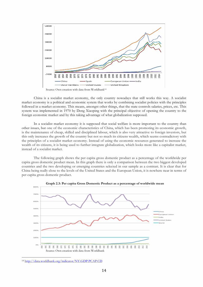
Graph 2.2: Per capita Gross Domestic Product

14


China is a socialist market economy, the only country nowadays that still works this way. A socialist

market economy is a political and economic system that works by combining socialist policies with the principles followed in a market economy. This means, amongst other things, that the state controls salaries, prices, etc. This system was implemented in 1970 by Deng Xiaoping with the principal objective of opening the country to the foreign economic market and by this taking advantage of what globalization supposed.

In a socialist market economy it is supposed that social welfare is more important to the country than

other issues, but one of the economic characteristics of China, which has been promoting its economic growth, is the maintenance of cheap, skilled and disciplined labour, which is also very attractive to foreign investors, but this only increases the growth of the country but not so much its citizens wealth, which seems contradictory with the principles of a socialist market economy. Instead of using the economic resources generated to increase the wealth of its citizens, it is being used to further integrate globalization, which looks more like a capitalist market, instead of a socialist market.

The following graph shows the per capita gross domestic product as a percentage of the worldwide per capita gross domestic product mean. In this graph there is only a comparison between the two biggest developed countries and the two developing or emerging countries selected in our sample as a contrast. It is clear that for China being really close to the levels of the United States and the European Union, it is nowhere near in terms of per capita gross domestic product.

Graph 2.3: Per capita Gross Domestic Product as a percentage of worldwide mean

Source: Own creation with data from Worldbank

14 http://data.worldbank.org/indicator/NY.GDP.PCAP.CD

15

One of the reasons for this disparity between countries could be the population, so it will be checked if

this might be the reason in the following section.

Evolut ion o f populat ion In the previous section there was an issue to clarify: if the low per capita gross domestic product of

China was due to the strategy followed by the country with wage levels or if it was due to the difference in population. To check this the elaboration the following graph, which shows the annual percentage growth of the population.

Graph 2.4: Population growth (annual %)


What it´s observed in the graph is that, although China´s population grew very quickly until 1971, then its growth rate decreases rather quickly, and today its population growth is under the rest of the country’s population growth analysed in this paper, with the exception of the European Union and Spain. So the lack of dispersion of wealth to the Chinese citizens must be due to de policy established of low wages to maintain a greater incentive for foreign investors and to favour companies with lower costs.

India on the contrary, has the highest population growth of all four countries, although it has a

downward trend, it is understood that its increase of gross domestic product is not being reflected in the per capita gross domestic product because of the increase of population. Spain is the country within our selected countries of study, with the least population growth, and this is also why it could reflect higher per capita gross domestic product.

Exports and Imports

Exports and imports are considered a measure of openness of the country or globalization. Several facts have already been mentioned before in this paper, and they will again be observable in the following graphs. The graphs are elaborated with data from the World Bank and show the exports of goods and services measured as a percentage of the GDP.

Graph 2.5: Imports of goods and services (% of GDP)

15 http://data.worldbank.org/indicator/SP.POP.TOTL

16


When looking at the imports it is seen that the United States has maintained a low, constant and stable

increase of its imports as a percentage of its GDP, being the country with the lowest percentage of imports with respect to its production of our sample of countries. There is a generalised trend though, that can be observed from the late 90´s to 2006 approximately, were it is observed a great increase for the majority of the representation of imports on the GDP.

Countries as for example Spain, and the UK are the countries that have a greater participation of

imports on their GDP. Generally it is seen that countries of the European Union have higher levels of imports. Spanish imports have increased greatly it importance within its GDP since 1960, increasing by nearly five times, whilst the UK has always had an important part of its GDP destined to imports, possibly due to its geographical isolation.

On the other hand, although China and India have increased their commercial openness, and this is seen

also in imports, especially in the first years of the 2000´s, both countries have seen a reduction of their imports in the last ten years.

Something similar happens to the exports of these countries seen in graph 2.6 seen as following. The

countries of the European Union continue to be the ones that more export in mean as percentage of their GDP. Spanish exports have also raised importance by five times as percentage of its GDP. Since the 2000´s India´s and China´s exports grow six times approximately since 1960, which has been an extraordinary phenomenon. China has decreased by almost 13 porcentual points, not being so affected Indi´s exports decreasing only by 5%.

Graph 2.6: Exports of goods and services (% of GDP)

17

Source: Own creation with data from Worldbank The reduction of exports can be due to the financial crisis that has affected our sample study countries. Another reason could be the increase of generalised GDP of these countries, representing these exports less quantity of the same. Many literates have considered exports and imports as a cause of the increase of inequality, this will be seen when the model is carried out.

Gini Index

The Gini Index is the most used resource for measuring inequality levels of countries accross the globe. It is a measurement of the income distribution and in some cases also of the wealth distribution among population that is performed throughout statistical methods. It generally refers to the inequality in income, as measuring wealth is very difficult. This index is ranged from 0 to 1, 0 being perfect distribution or equiality, and 1 being the contrary, perfect inequality. Although the possibility of overpassing this range above 1 is possible, because it takes into account the negative income or wealth. But the only case in which the gini index would have a zero value would be if each and every person resident of a country earned exactly the same.

The following graph shows the Gini Index of China, UK, India, US and Spain. The problem with this

index is that there is not enough data, and there is no calculation of this index for the European Union as a whole or at a worldwide level, and for some countries for example China and India which the WorldBank only has data of this index for two and one years respectively. Even the countries which have been years calculating this index as for example the US have not registered data in an annual basis, but only with several years of difference.

Graph 2.7: Gini Index (annual %)


16 http://data.worldbank.org/indicator/SI.POV.GINI

18

The range of the graph is in percentages from 0% to 100%. As it is observable from the graph, US´s inequality increases from 1986 to 1997 by 3 porcentual points, and since then is has oscillated around a mean of 40%, being its highest value of 41,75% in 2007, and the latest data being 41,06% in 2013. The US is the most inegalitarian country with the exception of China, confirming the assertion of some economists mentioned at the beginning of this paper that it is the developed country with highest income inequality. The United Kingdom on the contrary has seen a reduction of income inequality since 2004. Its gini index has reduced 3,65% in 8 years, which is approximately the same to US´s increase of inequality. The UK is the only developed country of our sample that has experienced this reduction. Spain for example, being also an European country, has seen an increase of 2,51% of its inequality index for the period 2004 to 2012. The mean gini index for both countries though is similar, around 34,5%, as the UK started with high levels of inequality and Spain with lower levels, and then have experienced contrary trends.

For China we only have available two data: 42,83% in 2008 and 42,16% in 2012. There has been a reduction of inequality in four years, but it should be considered that data could not be as reliable. Finally, India´s gini index is of 35,15% in 2011, but has the same issue of reliability of data as China.

The explanation of these levels could be due to the unemployment levels of each country. This data will

be observed in the following section.

Unemployment As it has been already mentioned before, an important variable to consider in the influence of the increase of inequality is the unemployment rate of a country. Obviously, if a country has higher levels of unemployment, there would be a higher proportion of the population of the country living in worst conditions, and this could be a reason of inequality increase. In the following graph there are illustrated a recollection of data from 1991 to 2016 of the total unemployment measured as a percentage of the total labour force. The first, and most astonishing evidence got from the graph are the level of unemployment of Spain. Not other country of our sample, not even the European Union mean or the OCDE members reach such levels, for the exception of the period 2004 to 2006 were the European Union has barely the same unemployment as Spain, but still below. In the Spanish trend it can be observed an M form, having its highest peaks in 1994, and 2013. From 1991 to 1994, there is a steep increase, due to the crisis suffered in this country. Since 1994, the unemployment rate starts to decrease rapidly, also incentivised by the creation of the real estate bubble that created a lot of employment. In 2007, the financial crisis bursts, and unemployment grows higher than in 1994. From 20013 to 2016, following with the country´s economic recovery, unemployment has reduced also, by 5%.

Graph 2.8: Unemployment, total (% of total labor force)


19

The rest of the samples of countries selected in this paper have lower, and similar unemployment rates. China and India for example, are the two countries that show a lower unemployment as a percentage of their labor force. Since 1980, when they focus on increasing the commercial openness of the country there is a reduction of unemployment especially for India. Another country with really low unemployment rates is the United States. This country is considered the most inegalitarian developed country, but it is definitely not due to its unemployment levels. It is observed that it increases in 2007, with the collapse of Lehman Brothers, but it reaches a maximum of 10% unemployment in 2010 and has seen a big increase of its employment since then, reaching a 4%. The United Kingdom follows the same trend as the US, although it never reached such high levels of unemployment during the crisis, the today have the same proportion of unemployment out of their total labor force. From the study of unemployment it is clear that for some countries unemployment can be an important factor when increasing the inequality levels, as for example Spain, that its employment lack of flexibility in the market has as a consequence a greater impact in the unemployment rates in times of crisis. For others, such as China, India or the US it is obvious that unemployment would not be a significant factor in the increase of inequality.

Inf lat ion

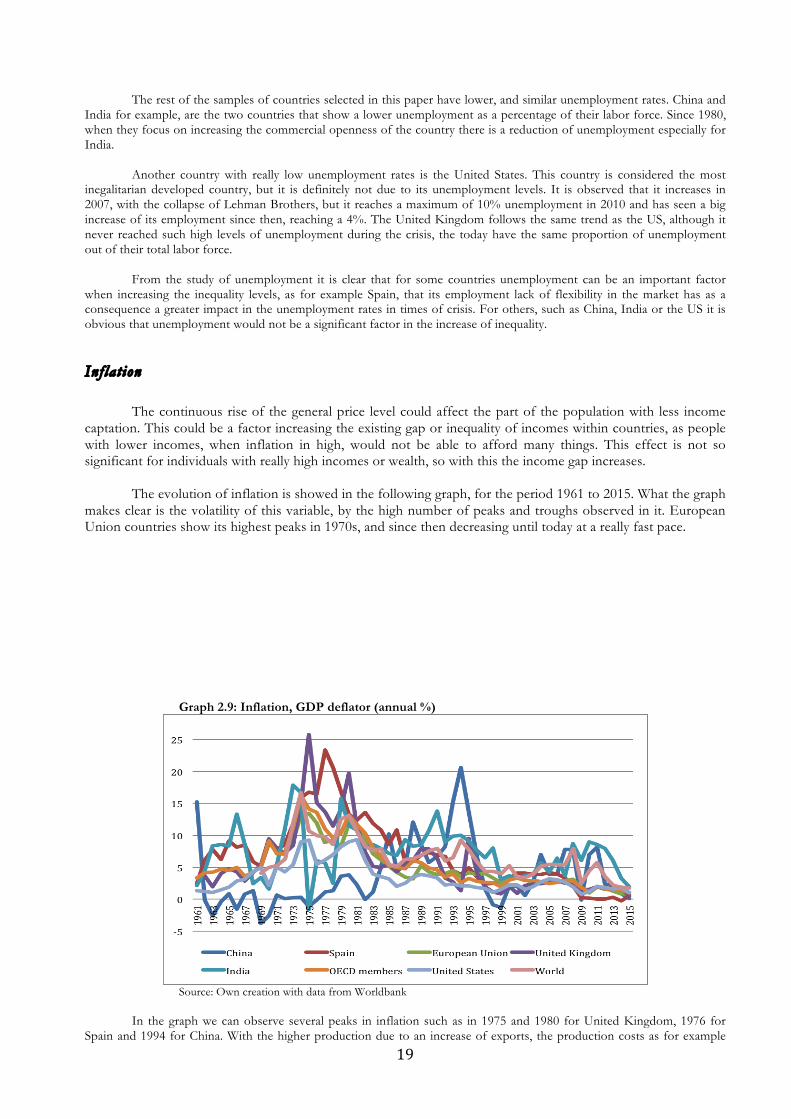
The continuous rise of the general price level could affect the part of the population with less income captation. This could be a factor increasing the existing gap or inequality of incomes within countries, as people with lower incomes, when inflation in high, would not be able to afford many things. This effect is not so significant for individuals with really high incomes or wealth, so with this the income gap increases. The evolution of inflation is showed in the following graph, for the period 1961 to 2015. What the graph makes clear is the volatility of this variable, by the high number of peaks and troughs observed in it. European Union countries show its highest peaks in 1970s, and since then decreasing until today at a really fast pace.

Graph 2.9: Inflation, GDP deflator (annual %)


In the graph we can observe several peaks in inflation such as in 1975 and 1980 for United Kingdom, 1976 for

Spain and 1994 for China. With the higher production due to an increase of exports, the production costs as for example

20

the costs of workforce, machinery, transport, which is very related also to a possible increase or decrease of costs derived from oil prices, etc., can increase. If these costs increase it could translate into higher product costs., and therefore increase inflation. This could be one of the reasons that explain the evolution of inflation.

The explanation of the last decade’s reduction and more or less stabilization of inflation are the monetary policies

being adopted with the objective of having an inflation close but below the 2% which is said to be the optimal level of inflation. This is why in the graph it can be observed how the countries of our sample´s inflation converge to be around 2%.

METHODOLOGY

For the carry out of this study a time series analysis would be the correct method in order to see the weight or influence each variable has in order to explain the total inequality. A time series is when data is collected for a variable during time at equidistant spaced time points.

Time series have a fundamental characteristic: the observations are not independent the one from the

other, and so when carrying out the analysis this will have to be taken into account, following the chronological temporal order of the observations of the sample data taken. This means that the statistical methods normally used for the independence of the observations are not valid for the analysis of time series, because the observations of a specific moment of time are dependent of values of the past series.

Depending on the observations any quantitative variable can be or discrete or continuous. Discrete variables are values within a given numeric group, but there are no intermediate values. Continuous variables on the other hand, can take any intermediate value between two observable values within an interval.

A temporal series can also be classified into deterministic or stochastic or random. If it is possible to

predict exactly the values it is said to be deterministic. If by contrary you can only partially predict the future using past observations but not in an accurate way, using a probability distribution to conclude the future values or predictions but being conditioned to past values the time series is said to be random or stochastic.

Panel data will be used, as the data collected are several variables for a period of time and for different

countries. This technique allows to realize a more dynamic analysis as it incorporates a temporal dimension of the data. It will allow identifying information as for example the individual effects and temporal effects.

Time Ser ies

Objectives of time series analysis

The objectives of using a time series analysis will be two: Descriptive and Prediction.

1. Descriptive

When studying a time series, you begin by drawing it, or in other words, by doing a graph with the data to analyse. From this we can identify the following:

- If there is an existence of trend in the data. - If the data has a stational factor. This is, when there is a trend in a specific month or months of the

period selected. - Identify existing outliers. These are abnormal values within our data, which can distort our results.

2. Prediction

The first objective of description is only an explanation of the past, but by using a time series analysis it is

also possible to do a prediction or forecast of the future. This will be possible when all the possible distortions of the data mentioned above are amended.

21

Components of a time series

The descriptive study of time series is based on decomposing the variation of the series into several basic

components. This method is not always the most accurate or appropriate, but it is useful when it comes to identifying a trend or periodicity in the series. This descriptive approach consists in identifying components that correspond to a long-term trend, a seasonal behaviour or a random component. The components to be identified are usually the following:

1. Trend: it is a long-term change that occurs in relation to an average level or, in other words, it is a long-term change in the mean.

2. Seasonality Effect: it occurs when the time series has a certain periodicity in a certain period repeatedly (annually, monthly, weekly, etc.). For example, in the stock market there is a saying “buy Monday, sell Friday”, it is called the “Monday effect”. It has been seen for a long period of time that the market has a tendency to fall every Monday. The contrary is seen in the prices of stocks on Friday, with the accumulation of rises in price of the week, it is said to be the best moment to sell, or buy short, to anticipate to “Monday effect”. If the seasonality in data is recognised and understood easily, and are measurable, they can be eliminated from the series.

3. Randomness: Once we have done the two previous steps of component identification, some random values remain. It is important not to remove trend and seasonality before this step. What it is intended is to identify the kind of random behaviour these residues present, using some kind of probabilistic model that describes them, as for example AR, MA, ARIMA, etc.

Of the three components mentioned above, the first two are deterministic components, while the latter

is a random component. Thus, it can be denoted that

Xt = Tt + Et + It Where:

- Tt is the trend, - Et is the seasonal component, which constitutes the deterministic part, - It is the noise or random part.

The randomness component is crucial when it comes to clarify the behaviour of a series in the long-term. It

is necessary to identify and isolate the random component and to study which probabilistic model is the most appropriate. Once we know this probabilistic model we will be able to know the behaviour of the series in the long term. This will be a reason for using Statistical Inference.

The ways to isolate this random component are normally the following: 1. Through a descriptive approach: Tt and Et are estimated and we obtain It as:

It = Xt - Tt - Et

2. Through the “Box-Jenkins” approach: By using transformations or filters it is possible to eliminate the

trend and seasonality from Xt, leaving only the probabilistic part. This probabilistic part is then fitted with parametric models.

Descriptive analysis of time series The first descriptive tool that will used is the time chart. The construction of a time chart is very useful when it comes to analyzing a time series because it enables us to observe its behavior. There are different types of time series, and each of them will be treated differently.

22

Classification of time series Time series can be classified into:

1. Stationary: A series is stationary when it is stable, in other words, when the mean and the variance of data are constant over time. This would be observed in a graph when the values of a series oscillate around a constant mean and variance, with respect to that mean also remains constant over time. Basically, it is a stable series over time, without any systematic variation of its values. However, it is also possible to apply the same methods to non-stationary series if they are previously transformed into stationary ones.

2. Non-Stationary: As contrary to stationary time series, non-stationary time series mean and variance

change over time. These variations in the average determine long term trend increases or decreases, so the series does not oscillate around a constant value.

Trendestimation In order to estimate the trend an assumption will be made: that it is a non-stationary series without a seasonal component, that is, that the series can be decomposed into

Xt = Tt + It For the sake of the estimation of Tt it must be assumed some hypothesis about its form. Several cases will be analysed:

a) Deterministic trend For this case the assumption it will by taken is that the trend follows a deterministic function. The simplest version of this function is a straight line, that is:

Tt = a + bt a and b being two constants to be determined. These constants will be estimated throughout a linear regression model and the variables Xt and the time t = 1, 2, 3, . . . , n. In this way, if the parameters â and b are estimated, then the irregular component would be:

It = Xt - â - t Graph 3.1: Series and linear tendency

Source: Halweb UC3M17 After estimating throughout a linear regression what it is obtained is a stationary series. It is not always possible to adjust the trend of the series by a straight line. If this is the case, the trend should be adjusted by a

17http://portal.uc3m.es/portal/page/portal/dpto_estadistica

23

polynomial or a curve that adjusts better, having to adjust a nonlinear regression. Another option would be to describe the trend in an evolutionary way or to differentiate the series.

b) Evolutionary trend (moving averages) An evolutionary trend is a trend that is assumed to be a function that evolves slowly over time and that can be approximated in very short intervals (for example 2 or 5 data). This can be done by a simple function of time, for example a line as we saw for deterministic trends, but now its coefficients change smoothly over time. We assume that the representation of the trend by a line is valid for three consecutive periods of time, t - 1, t, t + 1, and we represent the trends in the three consecutive periods as follows: Tt-1 = Tt - growth Tt Tt+1 = Tt + growth We now make the average of these three periods of time so that would result as follows:

mt = [(xt-1 + xt + xt+1 )]/3

mt = Tt + [It-1 + It + It+1] /3

As the irregular component has zero mean, the mean of these three values can be assumed to be unimportant against the trend. Mt would represent the trend at that moment of time. This operation is called the “triple moving average”. When doing this method or operation we lose the most antique and most recent observations. If were to calculate the moving averages of order 5, we will lose the two most recent observations and the two oldest observations.

c) Differentiation of the series The third and most generally used method for eliminating the trend is to make the assumption that the trend evolves slowly over time, so that at time t the trend should be close to the trend at time t-1. Hence, if we subtract from each value its previous value, the resulting series would be approximately free of trend. This method of eliminating the trend is called differentiation of the series, and it consists in moving from the original series xt to the series yt by:

yt = xt-xt-1

In this way, the differentiated series proves to be stationary.

Possible estimation problems: seasonality of data A seasonal component is a component os the series that is composed by oscillations that are prodcued in periods equal or less to one year and that they repeat themselves regularly throughout different years. If a year is considered as the period or repetition frame, fluctuations of the magnitude can be observed throughout its months, semester, trimester, cuatrimester, etc. The origin of this seasonal variations could be in factors as climatological seasons, cultural or tradition such as Christmas, vacacions, etc. For example, climatology affects the commercialization of icecreams, or summer clothing. When it is intended in the economic phenomena to analyze its real evolution we must eliminate the seasonal component since its fluctuations can distort the information provided by the series. That is, if we are analyzing sales of ice cream, we can not compare the volume of sales of the second quarter with the volume of sales of the third, because this variable has a strong seasonal component. The fact of being in the third quarter implies a higher level of sales, without which it can be considered an important fact. In order to compare two different quarters, we must eliminate the stational effect. This process is called the deseasonalisation of the observed series.

24

Graph 3.2: Seasonal data sample

Source: Halweb UC3M18 A series is deseasonalized when the seasonal factor and its effect is eliminated. This is done by eliminated from the value of the month or year that presents the seasonality the coefficient. For example, in a monthly seasonal effect, there would be 12 coefficients. In order to estimate them, the mean od the observations for each month has to be calculated (M1….M12). The seasonal coefficient would be:

Si = Mi-M for 1 = 1, ..., 12. Being M the total mean of the observations. The sum of all the seasonal coefficients must be zero. A deseasonalized series would look something as the following: Graph 3.3: Destationalised series

Source: Halweb UC3M19 In order to eliminate the trend, we have to apply the procedures mentioned in the previous section to the seasonally adjusted series. This could be done for example by means of differentiating the time series. This would result in a graph looking something as the following: Graph 3.4: Differentiated and destationalised series

Source: Halweb UC3M20

18 http://portal.uc3m.es/portal/page/portal/dpto_estadistica 19 http://portal.uc3m.es/portal/page/portal/dpto_estadistica20 http://portal.uc3m.es/portal/page/portal/dpto_estadistica

25

However it is observable that this series returns to have seasonaity issues. The problem here is that, in the moment we have differentiated it, the a seasonal effect has appeared again in the series. So it is better explained we will analyze some observations of the series x1, x2, · · ·, x13, x14 · · · To seasonally adjust the series, we performed the following transformation:

y1 =x1-E1 y2 =x2-E2 ···

y13 =x13-E1 y14 =x14-E2

··· So now, when we differentiate the series the result would be:

z2 = y2 -y1 = x2 -x1 - E2 +E1 = x2 -x1 -(E2 - E1) ···························

z14 = y14 -y13 = x14 - x13 - E2 +E1 = x14 - x13 - (E2 - E1) By this, a seasonal coefficient appears in the series: (E2 - E1). So it is possible to solve this problem, the trend of the seasonally adjusted series should be eliminated by the methods enumerated in the previous section. Another possible solution, which is the most appropriate, is to eliminate first the trend of the series and secondly to de-seasonalise the series. To verify that the series has a seasonal component, it can be checked by means of a time series graph. The following graph is an example of a graph that shows the seasonal coefficients of the series. As it can be observed these are higher for the months of July and August, and are lower for the months of December and February, which indicates that there is seasonality. Graph 3.5: Stational coefficients

Source: Halweb UC3M21 In the following graph an example of the seasonal decomposition of the series. The graph shows red horizontal lines representing each month, which show the mean of the series for each month. The vertical blue lines show the variation of the series for each month in different years. The graph shows a growing trend. Graph 3.6: Seasonal Decomposition


21 http://portal.uc3m.es/portal/page/portal/dpto_estadistica22http://portal.uc3m.es/portal/page/portal/dpto_estadistica

26

In the following chart year to year series are represented. We can see there is seasonality because the year to year variation of the different months is very similar, which indicates there is seasonality. Moreover, the twelve-year charts are in increasing order: the first year is below the second year, the second year is below the third year, and so on. This indicates that the series has an increasing tendency.

Graph 3.7: Annual Series


These charts would be useful in case that the simple inspection of the time chart is not enough.

Panel Data

Objectives of Panel Data Analysis

The principal objective of panel data is to capture the non-observable heterogeneity. This non-observable heterogeneity can be between economic agents as for time, as it cannot be detected throughout time series and cross-sectional data. This technique allows to realize a more dynamic analysis as it incorporates a temporal dimension of the data. It will allow identifying information as for example the individual effects and temporal effects. Individual effects are those that affect unequally to each of the agents of the sample, which are invariable with time, and affect in a direct way. Temporary effects on the other hand, are those that affect all variables equally and do not vary in time. These types of effects are usually associated to macroeconomic shocks, which can affect equally all variables of study.

Specification of a Panel Data Model The general specification for a panel data regression model would be the following24:

Yit = αit + Xitβ + uit , being i = 1, …., N and t= 1, …, T Where:

- i : is the individual or in this paper the country studied - t : is the period of time - α : is a vector of interceptors (the value of the dependent variable when all the rest of variables are

zero)of n parameters - β : is a vector of K parameters - Xit : is the ith observation at time t for the K explanatory variables. NxT will give the total sample of

observations. - uit : is the error term. This term has a further decomposition:

Uit = µi + δt + εit

23 http://portal.uc3m.es/portal/page/portal/dpto_estadistica 24 Burdisso, Tamara (1997)

27

Where:

o µi : represents the non-observable effects that differ between the studied units but not in time. o δt : represents the non-quantifiable effects that vary in time but not within the variables of the

sample taken. o εit : Is a purely random effect.

The most common or most used error term model when using panel data is the so-called “one way”, which makes the assumption that δt = 0. There are different variants to this “one way” model, which differ in the assumptions given to the µt. Generally these assumptions are the following:

1) µt = 0. This is the simplest assumption as it considers that there is no existence of non-observable heterogeneity between individuals or countries. Given this assumption, Uit would satisfy the general linear model and so the least-squares estimation method would produce the best estimators.

2) µt is a fixed and different effect for each country or individual. In this case, the unobservable heterogeneity is incorporated into the constant of the model.

3) µt is an unobservable random variable that varies between individuals but not over time. The other error term model is the so-called “two way”, which, as contrary to the “one way” model δt

≠ 0. This model is useful in order to capture the specific temporary effects or shocks that are not considered in this model.

Advantages and Disadvantages of the Panel Data Technique The panel data techinique counts with several advantages and disadvantages in comparison with the time series technique and the cross sectional technique. Between the uncountable number of each of them25 the most relevant are the following:

a) Advantages:

• Possibility to introduce a greater number of observations, increasing the degree of freedom and reducing the collineality between the explanatory variables and, ultimately, improving the efficiency of the estimations.

• This technique allows to capture the non-observable heterogeneity for both the individuals of the sample as for periods of time.

• It allows the application of a series of hypothesis testing in order to accept or reject the heterogeneity and how to capture it.

• This method makes the assumption that the individuals or countries are heterogenious, avoiding the bias that a cross sectional method could have.

• It allows the ellaboration and testing of complex behavioural models in comparison with the time series and cross section analysis.

• It enables a better way of studying the dynamics of adjustment processes. This is useful for studies as this one, for the observance of duration and permanence of certain levels of economic condition as for example unemplyment, poverty, wealth, etc.

b) Disadvantages:

• Generally, the disadvantages associated with the panel data technique are related with the information obtainance and processing of the statistical information of the individual units os the study, if this information is obtained from surveys or interviews or other sources that are not 100% representative.

25 For more advantages and disadvantages read Baltagi (1999) and Hsiao (1986)

28

DATA ANALYSIS

In order to find out the determinants of the Gini Index or income distribution inequality, this paper uses annual macroeconomic series for the period 2005 to 2015 because of the lack of information. For the recompilation of data the World Bank, OCDE and IMF have been, amongst others great and reliable resources. Yet it is true that many countries do not have a register of many variables, normally the ones that are less developed. In this section we will analyze the existing variables per country, which will then be used for our model. Some data related to the Gini Index are estimations from the WorldBank and other sources.

Inequality is defined by the Cambridge Dictionary as “the unfair situation in society when some people have more opportunities, money, etc. than other people”. “Although asset and wealth inequality is more appropriate than income inequality to represent the inequality in distribution, due to the lack of data on asset and wealth, this paper uses the Gini index for the measure of the inequality in distribution”.26 This sentence from the study of inequality in Korea is applicable to our study also, as the income distribution inequality Gini Index is the variable that we will try to explain.

For the index to represent globalization, a calculation of the share of trade volume has been calculation adding

exports and imports of the country in a year and then doing the division of the result by GNI. The rest of the

data is from the OCDE for European countries and from the World Bank for the United States, China and

India.

Table 1: Variable Definition Description Definition

Gini Index Gini Index of income distribution inequality (% from 0-100)

Inflation Yearly consumer price growth rate Population Total regardless of legal status or citizenship Unemployment rate Unemployment, total (% of total labor force) Foreign direct investment Total investment Openness Degree (Exports + Imports)/GNI

Source: own creation In order to see the determinants of income inequality a regression using the panel data methodology and from this some betas will be obtained. From this the impact of every variable will be observed throughout this beta and it will be possible to compare between the different groups of countries developed and emerging countries. In the following table the countries used for each group will be specified.

Table 2: Sample of countries selected

Developed countries Developing Countries United States

Austria Belgium Cyprus

Czech Republic Denmark Estonia Finland France

Germany Greece

Hungary Iceland Ireland

Italy Latvia

Lithuania Luxembourg

Malta Netherlands

Norway Poland

Portugal Slovakia Slovenia

Spain Sweden

United Kingdom

China India

Source: Own elaboration

26 Lee, Kim and Cin (2013), Empirical Analysis on the Determinants of Income Inequality in Korea, page 101

29

European countries Descriptive Statistics

Table 3: Descriptive statistics of European Countries

Source: Own creation from results from Gretl and data obtained from the Worldbank and the OCDE

United States Descriptive Statistics Table 4: Descriptive statistics of United States

Source: Own creation from results from Gretl and data obtained from the Worldbank

Emerging countries Descriptive Statistics Table 5: Descriptive statistics of China and India

Gini Population

OpennessDegree Unemployment Inflation

ForeignDirectInvestment

Mean 29,107 17594000 1,9499 8,5838 2,259 4906700000

Median 28,3 8351600 1,1973 7,564 2,1071 -300830000

Minimum 22,5 293580 0,52675 2,251 -4,4799 -1,9074E+11

Maximum 38,9 82501000 19,493 27,466 15,431 2,111E+11

Typ.Deviation 3,9256 23267000 2,7329 4,4637 2,2081 34984000000

C.V 0,13486 1,3224 1,4016 0,52002 0,97747 7,1298

Assimetry 0,33508 1,5123 4,2766 1,7357 1,8231 0,3732

Curtosis -0,95888 0,84533 19,074 3,7428 75571 10,945

Percentile5% 23,7 407610 0,62043 3,4329-

0,46054 -27880000000

Percentile95% 35,61 65309000 6,1526 17,753 5,6739 68183000000

Interquantilerange 6,5 14181000 0,94141 4,28 2,3095 1,2924E+11

Missingobservations 0 0 0 0 0 0

IntraD.T 3,7708 22733000 2,5583 4,4094 2,1666 34929000000

BetweenD.T 1,387 6476100 1,203 0,95741 0,56493 4252200000

NºObservations 297 297 297 297 297 297

Gini Population



Mean 47,109 17594000 1,9499 8,5838 2,259 4906700000

Median 46,9 8351600 1,1973 7,564 2,1071 -300830000

Minimum 46,3 293580 0,52675 2,251 -4,4799 -1,9074E+11

Maximum 48,1 82501000 19,493 27,466 15,431 2,111E+11

Typ.Deviation 0,61066 23267000 2,7329 4,4637 2,2081 34984000000

C.V 0,012963 1,3224 1,4016 0,52002 0,97747 7,1298

Assimetry 0,37365 1,5123 4,2766 1,7357 1,8231 0,3732

Curtosis -1,0779 0,84533 19,074 3,7428 75571 10,945

Interquantilerange 1 14181000 0,94141 4,28 2,3095 -27880000000


Gini Population



Mean 45,343 1,2836e+09 0,55707 4,0499 5,4196 -7,9510e+10

Median 47,7 1,3074e+09 0,54882 4,1470 5,1589 -4,9277e+10

Minimum 33 1,1443e+09 0,42691 3,49 -0,70295 -2,3165e+11

Maximum 51 1,3712e+09 0,71431 4,593 11,992 -4,6287e+09

30

Source: Own creation from results from Gretl and data obtained from the World Bank

ANALYSIS OF RESULTS In this section the results of the estimation of the regression will be exposed through the Gretl outputs that have been introduced in this paper. In the final part of this section a comparison between the coefficients of each variable and between countries will be made in order to analyse how each variable affects to a greater or lesser extent to the inegalitarian distribution of income.

European Countr i e s

The results of this analysis are a mean of the European countries selected, and so the possible effects are for the group of countries.

Modelo 1: con corrección de heterocedasticidad, utilizando 297 observaciones Variable dependiente: Gini

Coeficiente Desv. Típica Estadístico t Valor p

const 25.0195 0.444745 56.2560 <0.0001 *** Population 5.25795e-08 6.00885e-09 8.7503 <0.0001 *** Opennessdegree 0.0918425 0.0342199 2.6839 0.0077 *** Unemployment 0.291719 0.0247626 11.7807 <0.0001 *** Inflation 0.170032 0.0894533 1.9008 0.0583 * Foreign Direct Investment

−8.78558e-12 3.14686e-12 −2.7919 0.0056 ***

Estadísticos basados en los datos ponderados:

Suma de cuad. residuos 779.0398 D.T. de la regresión 1.636188 R-cuadrado 0.501855 R-cuadrado corregido 0.493296 F(5, 291) 58.63343 Valor p (de F) 4.43e-42 Log-verosimilitud −564.6277 Criterio de Akaike 1141.255 Criterio de Schwarz 1163.418 Crit. de Hannan-Quinn 1150.128

Estadísticos basados en los datos originales:

Media de la vble. dep. 29.10741 D.T. de la vble. dep. 3.925567 Suma de cuad. residuos 3413.585 D.T. de la regresión 3.424987

------------------------------------------------------------------------------------------------------------------------------

What it is observed from the results given by Gretl is that the variables population, openness degree or globalization, unemployment, and inflation increase the inequality in the distribution of incomes of Europe, having them all a very significant effect, being inflation the less, but still significant variable. Foreign Direct Investment has a negative impact over the Gini coefficient, as for every unit it increases the coefficient decreases −8.78558e-12 units. The model explains a 50,19% of the Gini coefficient.

Typ.Deviation 5,9786 6,8889e+07 0,082007 0,39026 3,5021 7,4137e+10

C.V 0,13185 0,053669 0,14721 0,096364 0,6462 0,93243

Assimetry -1,3869 -0,63364 0,42023 -0,14741 0,2767 -0,72888

Curtosis 0,17335 -0,82148 -0,71406 -1,4822 -0,85892 -0,80467

Interquantilerange 2,5 1,1253e+08 0,43173 3,496 -0,38112 1,2209e+11


IntraD.T 4,1781 4,2089e+07 0,075258 0,30359 2,2873 4,0269e+10

BetweenD.T 7,5345 7,6414e+07 0,050411 0,35098 0,3,7287 8,6860e+10

31

From these results the United Kingdom might be taking the correct decision when deciding to decrease its commercial and population opening, as both variables would mean that if one unit of each increases, the Gini coefficient would increase by 0,0918 units.

United Sta te s

The model in the case of United States´ regression explains a 93% of the variability of the Gini coefficient, which is amazingly high.

Modelo 1: con corrección de heterocedasticidad, utilizando 297 observaciones

Variable dependiente: Gini

Coeficiente Desv. Típica Estadístico t Valor p Population 1.79470e-07 7.06578e-09 25.40 2.45e-07 *** Openness degree −24.2511 5.91732 −4.098 0.0064 *** Unemploymen −0.197130 0.0749912 −2.629 0.0391 ** Inflation 0.707564 0.0773722 9.145 9.62e-05 *** Foreign Direct Investment

3.82960e-12 2.10718e-12 1.817 0.1190

Estadísticos basados en los datos ponderados:

Suma de cuad. residuos 8.287306 D.T. de la regresión 1.175252 R-cuadrado 0.929749 R-cuadrado corregido 0.882914 F(5, 291) 15.88150 Valor p (de F) 0.002098 Log-verosimilitud −14.05089 Criterio de Akaike 38.10177 Criterio de Schwarz 40.09125 Crit. de Hannan-Quinn 36.84769

Estadísticos basados en los datos originales: Media de la vble. dep. 47.10909 D.T. de la vble. dep. 0.610663 Suma de cuad. residuos 1.331571 D.T. de la regresión 0.471093

------------------------------------------------------------------------------------------------------------------------------ For the United States case we see different results. In this case the Foreign Direct Investment is found

not to affect United States´ income distribution inequality, as it results not to be significant. Population once again affects positively the inequality, increasing it, as well as Inflation, which for every unit it increases, the Gini index increases in 0,707564 units.

Contrary to what it was found for European countries the variable of globalization, openness degree and

unemployment are significant factors that reduce income distribution inequality. For example, if unemployment increases in one unit, the Gini coefficient would decrease by 0,197 units, and if the openness degree increases in one unit, it would decrease 24,25 units. This result would be a signal that the protectionist measures being taken by the United States Government would have a negative effect for the country, as it would very possibly increase its inequality in terms of income distribution.

Inflation is a variable that for Blinder and Esaki (1978) is only a “progressive tax in that the poor and middle classes lose relatively less than the rich”, but this is not what our results for both developed groups of countries show, as for both an increase of one unit of inflation would result in an increase of 0,877596 units of the Gini Index.

Emerg ing countr i e s China and India´s mean determinant coefficients show different results than the previously seen for

European countries mean and United States.

Modelo 2: con corrección de heterocedasticidad, utilizando 15 observaciones Variable dependiente: Gini

Coeficiente Desv. Típica Estadístico t Valor p

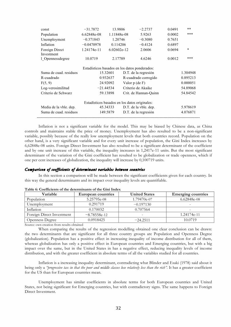
32

const −31.7872 13.9806 −2.2737 0.0491 ** Population 6.62848e-08 1.11848e-08 5.9263 0.0002 *** Unemployment −0.371843 1.20746 −0.3080 0.7651 Inflation −0.0470978 0.114206 −0.4124 0.6897 Foreign Direct Investment

1.24174e-11 6.02602e-12 2.0606 0.0694 *

l_Opennessdegree 10.0719 2.17789 4.6246 0.0012 ***

Estadísticos basados en los datos ponderados: Suma de cuad. residuos 15.32601 D.T. de la regresión 1.304948 R-cuadrado 0.932637 R-cuadrado corregido 0.895213 F(5, 9) 24.92092 Valor p (de F) 0.000051 Log-verosimilitud −21.44534 Criterio de Akaike 54.89068 Criterio de Schwarz 59.13898 Crit. de Hannan-Quinn 54.84542

Estadísticos basados en los datos originales:

Media de la vble. dep. 45.34333 D.T. de la vble. dep. 5.978619 Suma de cuad. residuos 149.5879 D.T. de la regresión 4.076871

------------------------------------------------------------------------------------------------------------------------------

Inflation is not a significant variable for the model. This may be biased by Chinese data, as China controls and maintains stable the price of money. Unemployment has also resulted to be a non-significant variable, possibly because of the really low unemployment levels that both countries record. Population on the other hand, is a very significant variable and for every unit increase of population, the Gini Index increases by 6,62848e-08 units. Foreign Direct Investment has also resulted to be a significant determinant of the coefficient and by one unit increase of this variable, the inequality increases in 1,2417e-11 units. But the most significant determinant of the variation of the Gini coefficient has resulted to be globalization or trade openness, which if one per cent increases of globalization, the inequality will increase by 0,100719 units.

Compar ison o f co e f f i c i en t s o f de t e rminant var iab l e s be tween countr i e s In this section a comparison will be made between the significant coefficients given for each country. In

this way the general determinants and its impact over inequality levels are quantifiable. Table 6: Coefficients of the determinants of the Gini Index

Variable European countries United States Emerging countries Population 5.25795e-08 1.79470e-07 6.62848e-08 Unemployment 0.291719 −0.197130 - Inflation 0.170032 0.707564 - Foreign Direct Investment −8.78558e-12 - 1.24174e-11 Openness Degree 0.0918425 −24.2511 10.0719

Source: own creation from results obtained When comparing the results of the regression modelling obtained one clear conclusion can be drawn:

the two determinants that are significant for all three country groups are Population and Openness Degree (globalization). Population has a positive effect in increasing inequality of income distribution for all of them, whereas globalization has only a positive effect in European countries and Emerging countries, but with a big impact over the same, but in the United States in has a negative effect, reducing inequality levels of income distribution, and with the greater coefficient in absolute terms of all the variables studied for all countries. Inflation is a increasing inequality determinant, contradicting what Blinder and Esaki (1978) said about it being only a “progressive tax in that the poor and middle classes lose relatively less than the rich”. It has a greater coefficient for the US than for European countries mean. Unemployment has similar coefficients in absolute terms for both European countries and United States, not being significant for Emerging countries, but with contradictory signs. The same happens to Foreign Direct Investment.

33

Limita t ions o f our proposed mode l It is important to mention that there may be problems of reverse causality. That is, GDP growth can be interpreted as a variable that affects, through our estimated beta, inequality. It can also be argued that changes in inequality stimulate or slow down economic growth.

StatisticsHowTo defines reverse causality as follows: “Reverse causality means that X and Y are associated, but not in the way you would expect. Instead of X causing a change in Y, it is really the other way around: Y is causing changes in X”.

There is a link between, on the one hand, international financial integration and financial development and, on the other, between financial development and economic growth. However, this does not necessarily imply that the first factor constitutes the cause of the latter is causal to the third. The policy of opening a country's finances may be endogenous or dependent, to some extent, on the development of the financial system and this can be, in turn, endogenous to economic growth. The existence of endogeneity leads us to determine the direction of causality. Figure 1: Factors That Enable International Financial Integration Contributory to Economic Growth

Reverse causality

Looking to the diagram from left to right, the first relationship is between the international financial integration and the financial development. It is normal for governments to ensure the liberalization of financial markets, as well as promoting their integration when to circumstances have happened or are about to happen: first, as a response to unusually high levels of demand for investment in the previous years and second, as an anticipation of shocks to marginal productivity of capital. If the governments decided to liberalise the financial markets this would cause the rate of growth of real investment to increase, especially due to the expectations generated. The positive expectations on marginal productivity of capital would cause both an investment growth and a financial liberalization; therefore, although there is an existing correlation between these two concepts, the financial liberalization would not be the cause of the investment increase.

In the second relationship, the financial development may influence the economic growth, and the other way round, having the economic growth an influence over financial development, causing a possible simultaneity bias. The possible problem that could arise from this is what is called an inverse causality to that posed in Figure X. It is also possible for the causality not to exist, and so both effects can be conduced by common omitted variables (Rajan and Zingales, 1998).

If for example we started at a specific period of time, the level of financial development at the beginning

of this period predicts the economic growth rate of the years yet to come. (King and Levine, 1993b; Levine and

Factors surrounding financial integration

Effects of financial integration

Channels through which financial integration causes economic growth

Financial liberalization Technological development

Financial engineering Institutional investments

Competition Induction to the adoption of better

policies

Direct and Indirect Barriers International Risk Diversification

Possibilities Liquidity

Bank Development International Capital flows

Cost of capital Allocation efficiency

Level of financial development

Inte

rna

tion

al f

ina

nc

ial I

nte

gra

tion

Eco

no

mic

gro

wth

Distortions Distortions

34

Zervos, 1998b). So these two authors believed that this factor could be used for doing forecasts about the future economic growth rate. From what these two authors tell us it could be concluded not only that finance is conditioned by the economic activity, but also the level of financial development conditions the future economic growth.

However, there is a problem with the previous statement, and it is that this approach does not properly

captures the bias in simultaneity, and therefore, does not determine the existence of causality in the relationship mentioned. Financial development is able to predict growth simply because the financial system is developed in anticipation to future economic growth. It could be thought that if financial development occurs ahead of time, it cannot be produced as a response to necessities of the real economy, but due to or as a cause of economic growth.

However, this argument is not valid formally because financial development can be an early indicator of growth, that is, the financial markets can anticipate the increase of economic activity and develop in anticipation of this activity. Financial markets capitalize on the current value of growth opportunities, while financial institutions lend more capital if they believe the economy will grow. Thus, financial development can simply be an early indicator and not a causal factor (Rajan and Zingales, 1998).

In this sense, some authors have demonstrated that the positive relationship between financial development and economic growth is not due to the simultaneity bias (Levine, 1998 and Levine, 1998). 1999, Levine et al., 2000), but there is a causality in the direction proposed in Figure 1. Now, studies based on samples and different periods have observed that there may be bi-directionality in the causality between both factors (Ahmed and Ansari, 1998, Neusser and Kugler, 1998), although depending on the characteristics of the countries analysed the intensity of causality varies in one way or another. With regard to the present work, the remarkable thing is that there is not only causality in the direction and the growth is higher in countries with greater financial development (Alfaro et al, 2004; M, 2004).

CONCLUSIONS This paper reviews the trends of some of the main macroeconomic variables of the countries of greater interest of our sample and investigates the determinants influencing the variance of the Gini coefficients as representative of inequality measurement. The trend analysis is for a period between 1980 and 2015, but the regression model estimation only takes values for the time period 2005 to 2015 due to the lack of information of some variables.

35

On the level of globalization and poverty, the situation between China and the EU is different. In the Chinese economy, the problems of poverty come from the increasingly liberalized economic activity. The authorities act step by step, to fight against this poverty and adapt their policies to the conjuncture. In the EU, poverty problems are less serious, but they are structural. That is to say, in the structure of economies, a non-negotiable part of the population is left out of the process of production and income generation. The institutions try to act with social policies that are insufficient until today.

The empirical results observed when comparing the results of the regression modelling obtained one clear conclusion can be drawn: the two determinants that are significant for all three country groups are Population and Openness Degree (globalization). Population has a positive effect in increasing inequality of income distribution for all of them, whereas globalization has only a positive effect in European countries and Emerging countries, but with a big impact over the same, but in the United States in has a negative effect, reducing inequality levels of income distribution, and with the greater coefficient in absolute terms of all the variables studied for all countries. Inflation is an increasing inequality determinant, contradicting what Blinder and Esaki (1978) said about it being only a “progressive tax in that the poor and middle classes lose relatively less than the rich”. It has a greater coefficient for the US than for European countries mean. Unemployment has similar coefficients in absolute terms for both European countries and United States, not being significant for Emerging countries, but with contradictory signs. The same happens to Foreign Direct Investment.

It is important to mention that there may be problems of reverse causality. That is, GDP growth can be interpreted as a variable that affects, through our estimated beta, inequality. It can also be argued that changes in inequality stimulate or slow down economic growth. In terms of the questions, which were aimed to answer at the beginning of this end of master project about, if globalization was causing inequality the answer would be that it depends of the case, but generally it does. This leads to the second question, which was aimed to answer: are the United States and the United Kingdom taking a good decision leaning towards protectionist measures? Once again it depends. For European countries as a mean, it was found that the globalization representative variable increased income distribution inequality, and by looking at this result it would be a good idea in terms of reducing inequality, but for the US it was found the opposite result, as this variable reduced its Gini coefficient, being the wrong decision to take.

REFERENCES

Books Arnaud Costinot y Andrés Rodríguez-Clare en el Handbook of International Economics, volumen 4. El título, Trade Theory with Numbers: Quantifying the Consequences of Globalization,

36

JEFFREY G. WILLIAMSON, (Capítulo 5) Globalización: ¿Hacia un mundo más desigual? El desarrollo económico mundial en perspectiva histórica. Cinco siglos de revoluciones industriales, globalización y desigualdad. Santiago Colmenares (traductor y coordinador científico). Prensas de la universidad de Zaragoza. Thomas Piketty, Capital in the Twenty – First Century

Box, G.E.P., Jenkins, G.M., Reinsel, G.C. (1994), Time Series Analysis – Forecasting and Control (3rd edition), Prentice Hall.

Reinsel, G.C. (1997), Elements of Multivariate Time Series Analysis (2nd edition), Springer.

Brooks, C. (2002), Introductory Econometrics for Finance, Cambridge.

Davidson, R., MacKinnon, J.G. (2004), Econometric Theory and Methods, Oxford.

Beck, T y Levine, R (2004): “Stock Markets, Banks, and Growth: Panel Evidence”, Journal of Banking and Finance, 28, 423-442

Bekaert, G ; Harvey, C R y Lundblad, D (2005): “Does Financial Liberalization Spur Growth?”, Journal of Financial Economics, 77(1), 3-55

Bekaert, G ; Harvey, C R ; Lundblad, C y Siegel, S (2004): “Global Growth Opportunities and Market Integration”, National Bureau of Economic Research (NBER) Working Paper, 10990, Cambridge, 1-47.

Bencivenga, V.R. y Smith, B.D. (1991): “Financial Intermediation and Endogenous Growth”, Review of Economic Studies, 58(2), 195-209.

Chen, Z. y Khan, M.S. (1997): “Patterns of Capital Flows to Emerging Markets: A Theoretical Perspective”, International Monetary Fund (IMF) Working Paper, 13, 1-32

De Gregorio, J. y Guidotti, P.E. (1995): “Financial development and Economic Growth”, World Development, 23(3), 433-448

Demirgüç-Kunt, A. y Levine, R. (1996a): “Stock Market, Corporate Finance, and Economic Growth: An Overview”, World Bank Economic Review, 10, 223-240

Demirgüç-Kunt, A. y Levine, R. (1996b): “Stock Market Development and Financial Intermediaries: Stylized Facts”, World Bank Economic Review, 10(2), 291-322.

Devereux, M.B. y Smith, G.W. (1994): “International risk sharing and Economic Growth”, International Economic Review, 35(4), 535-550

Edwards, S (2001): “Capital Mobility and Economic Performance: Are Emerging Economies Different?”, National Bureau of Economic Research (NBER) Working Paper, 8076, Cambridge, 1-32

Fischer, S (2003): “Globalization and Its Challenges”, American Economic Review, 93(2), 1-30.

Gupta, N y Yuan, K (2005): “On the Growth Effects of Liberalizations”, Social Science Research Network (SSRN) Working Paper, junio, 1-34

Kaminsky, G L y Schmukler, S L (2003): “Short-run Pain, Long-Run Gain The Effects of Financial Liberalization”, International Monetary Fund (IMF) Working Paper, 34, 1-59.

Kose, M A ; Prasad, E M y Terrones, M E (2005): “Growth and Volatility In an Era of Globalization”, IMF Staff Papers, 52, 31-63

Kraay, A. (1998): “In Search of the Macroeconomic Effect of Capital Account Liberalization”, World Bank Group Manuscript,

37

1 de octubre, 1-45

Levine, R ; Loayza, N y Beck, T (2000): “Financial Intermediation and Growth: Causality and Causes”, Journal of Monetary Economis, 46, 31-77

Love, I (2001): “Financial Development and Financing Constraints: International Evidence From the Structural Investment Model”, Social Science Research Network (SSRN) Working Paper, 1-49.

Lusinyan, L (2002): “International Capital Flows, Economic Growth and Financial Market Efficiency”, European University Institute Working Paper, Department of Economics, 20, 1-36

Mclean, B y Shrestha, S (2002): “International Financial Liberalization and Economic Growth”, Reserve Bank of Australia Research Discussion Paper, 03, Economic Research Department, 1-24

Merton, R.C. (1992): “Financial Innovation and Economic Performance”, Journal of Applied Corporate Finance, 4(4), 12-22

Neusser, K. y Kugler, M. (1998): “Manufacturing Growth and Financial Development: Evidence From OECD Countries”, Review of Economics and Statistics, 80, 638-646

Obstfeld, M. (1994): “Risk Taking, Global Diversification and Growth”, American Economic Review, 84(5), 1.310-1.329.

Prasad, E ; Rogoff, K Wei, S y Kose, M A (2003): “Effects of Financial Globalization on Developing Countries: Some Empirical Evidence”, International Monetary Fund (IMF) Occasional Paper, 220, septiembre, 1-86

Rajan, R.G. y Zingales, L. (1998): “Financial Dependence and Growth”, American Economic Review, 88, 559-586.

Schmukler, S L y Zoido-Lobatón, P (2001): “Financial Globalization: Opportunities and Challenges for Developing Countries”, World Bank Working Paper, 30 de mayo, 1-47

Shirakawa, M; Okina, K. y Shiratsuka, S. (1997): “Financial Market Globalization: Present and Future”, Institute for Monetary and Economic Studies Discussion Paper Series, 56

Stulz, R M (2005): “The Limits of Financial Globalization”, Journal of Finance, 60(4), 1.595-1.638.

Wacziarg, R y Welch , K (2003): “Trade Liberalization and Growth: New Evidence”, National Bureau of Economic Research (NBER) Working Paper, 10152, Cambridge, 1-90.

Azizur, Rahman y Riskin, Carl “Inequality and Poverty in China in the Age of Globalization”, 2001

Begg Iain, Draxler Juraj y Mortensen Jorgen, “Is Social Europe Fit for Globalisation? A study of the social impact of

globalisation in the European Union”, 2008

Forum OCDE “Growing Income Inequality in OECD Countries: What drives it and How Can Policy Tackle it?” Paris,

mayo 2011

Benjamin, Dwayne «Income inequality during China's Economic Transition», China's Great Transformation, Cambridge,

2008

De la Dehesa, Guillermo « Globalización, desigualdades y pobreza », Ediciones Alianza Editorial,

2003

Kaplinsky, Raphael “Globalization, Poverty and Inequality”, 2005

38

Milanovic Branko “Worlds Apart: Measuring Global and International Inequality” Princeton University Press, 2005

Wu Yi y Wei Shang-Jin «Globalization and Inequality: Evidence from Within China», Cambridge, Massachusetts, National

Bureau of Economic Research, 2001

Reports International Monetary Fund: “World Economic Outlook” April 2017 Kuhn and Ríos-Rull, 2013 Update on the U.S. Earnings, Income, and Wealth Distributional Facts: A View from Macroeconomics

Lee, Kim and Cin, Empirical Analysis on the Determinants of Income Inequality in Korea, April 2013, International Journal of Advanced Science and Technology

Artic l es

Globalización y desigualdad – Libertad González 17/02/2017 Pikkety´s Inequality Story in Six Charts – John Cassidy March 26, 2014 http://www.newyorker.com/news/john-cassidy/pikettys-inequality-story-in-six-charts

Internet webpages https://madeinchina2013.wordpress.com/2013/03/29/50/ http://elespaciohumanizado.wikispaces.com/GLOBALIZACIÓN+Y+DESIGUALDADES+TERRITORIALES+Y+SOCIALES http://www.statisticshowto.com/reverse-causality/ http://elpais.com/diario/2003/01/07/internacional/1041894001_850215.html http://www.politicaexterior.com/articulos/economia-exterior/las-tic-en-africa-sector-economico- en-alza-y-herramienta-social/ http://www.who.int/mediacentre/factsheets/fs355/es/ http://www.alternatives-economiques.fr/mondialisation-et-inegalites---parc_fr_art_1_26796.html http://www.robert-schuman.eu/fr/questions-d-europe/0296-l-europe-dans-la-mondialisation- risques-et-atouts http://ec.europa.eu/public_opinion/archives/eb/eb73/eb73_vol2_fr.pdf http://europa.eu/rapid/press-release_MEMO-13-631_es.htm https://www.wsws.org/es/articles/2016/12/24/eeuu-d24.html http://wid.world/world/#sfiinc_p99p100_z/US;CN;GB;IN;ES/last/eu/k/p/yearly/s/false/3.4125000000000005/30/curve/false http://www.bccr.fi.cr/investigacioneseconomicas/metodoscuantitativos/Tecnica_datos_panel,_una_guia_para_su_uso_e_interpretacion.pdf

ANNEX

39

Variab le s used in the r egr e s s ion

European Countries

Country YearGini(%) Population

Opennessdegree

Unemployment(%) Inflation


Austria 2005 26,3 8.201.359 1,1424380 5,627999783 2,304765879 193822310,2

Austria 2006 25,3 8.254.298 1,1900711 5,243000031 1,449618451 5581271419

Austria 2007 26,2 8.282.984 1,3579253 4,857999802 2,168599053 10177102307

Austria 2008 27,7 8.307.989 1,3377958 4,127999783 3,21592066 21598079156

Austria 2009 27,5 8.335.003 1,0616790 5,301000118 0,506312509 1264455428

Austria 2010 28,3 8.351.643 1,1142370 4,820000172 1,813535031 7680910617

Austria 2011 27,4 8.375.164 1,2937318 4,56400013 3,266938912 15145339304

Austria 2012 27,6 8.408.121 1,2194936 4,864999771 2,485675087 13230033894

Austria 2013 27,0 8.451.860 1,1674063 5,335000038 2,000157493 10578469481

Austria 2014 27,6 8.506.889 1,1973190 5,619999886 1,605805605 -2589378871

Austria 2015 27,2 8.576.261 1,1111807 5,72300005 0,896567005 7232905919

Belgium 2005 28,0 10.445.852 1,7008171 8,43999958 2,784303489 -1139201857

Belgium 2006 27,8 10.511.382 1,7746598 8,24600029 1,79094071 -8688143202

Belgium 2007 26,3 10.584.534 2,0035165 7,458000183 1,822063641 -13095644187

Belgium 2008 27,5 10.666.866 2,0769463 6,975999832 4,489444205 32847748785

Belgium 2009 26,4 10.753.080 1,6338175 7,907999992 -0,049480455 -61786380962

Belgium 2010 26,6 10.839.905 1,6602054 8,291999817 2,189218922 -53443937320

Belgium 2011 26,3 11.000.638 1,9110507 7,139999866 3,531058241 -31908772417

Belgium 2012 26,5 11.094.850 1,8128870 7,541999817 2,838723095 27171589994

Belgium 2013 25,9 11.161.642 1,8612646 8,425000191 1,11223458 4855245259

Belgium 2014 25,9 11.180.840 1,9185830 8,522999763 0,34 7408952889

Belgium 2015 26,2 11.237.274 1,6544647 8,482000351 0,558102452 8974302409

Cyprus 2005 28,7 733.067 1,1313911 5,303999901 2,558451986 -614353041,3

Cyprus 2006 28,8 744.013 1,1585246 4,543000221 2,495874931 -974613952,3

Cyprus 2007 29,8 757.916 1,3794412 3,921999931 2,372492743 -1032465697

Cyprus 2008 29,0 776.333 2,1008251 3,654999971 4,669171081 2291496850

Cyprus 2009 29,5 796.930 1,8884677 5,363999844 0,374079976 -2069640308

Cyprus 2010 30,1 819.140 2,0507378 6,263000011 2,381258363 3483638096

Cyprus 2011 29,2 839.751 2,0374537 7,855999947 3,289449396 -4209030710

Cyprus 2012 31,0 862.011 1,7091509 11,79500008 2,389768958 2490289577

Cyprus 2013 32,4 865.878 1,7197085 15,87100029 -0,400053061 -461198672,6

Cyprus 2014 34,8 858.000 1,8044489 16,08799934 -1,354988854 -1638538251

Cyprus 2015 33,6 847.008 1,5557839 14,90799999 -2,096997691 9385180818Czech

Republic 2005 26,0 10.198.855 1,4272957 7,927000046 1,846170702 -11628846667Czech

Republic 2006 25,3 10.223.577 1,5337525 7,147999763 2,528104997 -4042665554Czech

Republic 2007 25,3 10.254.233 1,7118075 5,320000172 2,927443471 -8963737209Czech

Republic 2008 24,7 10.343.422 1,7148945 4,392000198 6,350986289 -2257634944Czech

Republic 2009 25,1 10.425.783 1,3346607 6,662000179 1,044811886 -1951523283Czech

Republic 2010 24,9 10.462.088 1,4564850 7,278999805 1,408717924 -4918465928Czech

Republic 2011 25,2 10.486.731 1,6869283 6,710999966 1,936389149 -2592551186

40

CzechRepublic 2012 24,9 10.505.445 1,6431344 6,978000164 3,299073139 -6180626420Czech

Republic 2013 24,6 10.516.125 1,6598243 6,953000069 1,434726602 379979406,5Czech

Republic 2014 25,1 10.512.419 1,8069355 6,107999802 0,337186898 -4014433931Czech

Republic 2015 25,0 10.538.275 1,6744417 5,046000004 0,344782438 1085936218

Denmark 2005 23,9 5.411.405 1,0646884 4,829999924 1,808805419 3372185289

Denmark 2006 23,7 5.427.459 1,1289659 3,897000074 1,890073335 5726180176

Denmark 2007 25,2 5.447.084 1,2634637 3,801000118 1,714031313 8185821306

Denmark 2008 25,1 5.475.791 1,3178103 3,434000015 3,399474759 12133094650

Denmark 2009 26,9 5.511.451 0,9936434 6,006999969 1,326372231 1942771757

Denmark 2010 26,9 5.534.738 1,0076988 7,464000225 2,297730121 11500336082

Denmark 2011 26,6 5.560.628 1,1338244 7,572999954 2,758682261 -760896205,7

Denmark 2012 26,5 5.580.516 1,0838723 7,526000023 2,397914857 5210202439

Denmark 2013 26,8 5.602.628 1,1223457 6,997000217 0,78907178 10625216770

Denmark 2014 27,7 5.627.235 1,1515250 6,589000225 0,56402054 3732464397

Denmark 2015 27,4 5.659.715 1,0472347 6,168000221 0,452034154 5399350145

Estonia 2005 34,1 1.358.850 1,7973752 8,032999992 4,089689921 -2253768927

Estonia 2006 33,1 1.350.700 1,8399840 5,914999962 4,42991487 -675619881,8

Estonia 2007 33,4 1.342.920 1,9735028 4,592000008 6,597638594 -977361941,1

Estonia 2008 30,9 1.338.440 1,9192050 5,454999924 10,36560303 -618602267,5

Estonia 2009 31,4 1.335.740 1,3304822 13,54800034 -0,084776494 -503213311,9

Estonia 2010 31,3 1.333.290 1,6165243 16,70700073 2,975580329 -1351125196

Estonia 2011 31,9 1.329.660 2,0329793 12,32800007 4,977614784 -2487904958

Estonia 2012 32,5 1.325.217 1,9128007 10,02099991 3,934921578 -506081682,4

Estonia 2013 32,9 1.320.174 1,9008475 8,630999565 2,788496796 -236392968,6

Estonia 2014 35,6 1.315.819 1,8755574 7,352000237 -0,144815519 -763249727,6

Estonia 2015 34,8 1.314.870 1,5504024 6,186999798 -0,456766653 185776472,2

Finland 2005 26,0 5.236.611 0,8752698 8,383999825 0,861059229 -390440069,1

Finland 2006 25,9 5.255.580 0,9613477 7,718999863 1,566666667 -2838700281

Finland 2007 26,2 5.276.955 1,0823134 6,854000092 2,510666229 -5461934622

Finland 2008 26,3 5.300.484 1,1243032 6,368999958 4,065951657 10734709538

Finland 2009 25,9 5.326.314 0,8046825 8,25 0,00061529 4918451853

Finland 2010 25,4 5.351.427 0,8485491 8,394000053 1,210357625 2766177847

Finland 2011 25,8 5.375.276 0,9542537 7,781000137 3,416809034 2455848423

Finland 2012 25,9 5.401.267 0,9270037 7,68900013 2,808332326 3445292138

Finland 2013 25,4 5.426.674 0,9299045 8,19299984 1,478288133 -2302767992

Finland 2014 25,6 5.451.270 0,9339756 8,663000107 1,041200006 -17443282593

Finland 2015 25,2 5.471.753 0,7922615 9,376000404 -0,207164371 -17532304205

France 2005 27,7 62.772.870 0,6584308 8,946000099 1,735587081 33679643405

France 2006 27,3 63.229.635 0,7042172 8,93599987 1,68372645 51416740927

France 2007 26,6 63.645.065 0,7756360 8,053999901 1,488073528 48464051603

France 2008 29,8 64.007.193 0,7864163 7,484000206 2,813915043 67954539784

France 2009 29,9 64.350.226 0,6094079 9,147000313 0,088084169 70242406326

France 2010 29,8 64.658.856 0,6445054 9,303999901 1,529639382 33683933606

France 2011 30,8 64.978.721 0,7266257 9,248000145 2,117486809 20268741865

France 2012 30,5 65.276.983 0,7066354 9,81499958 1,9556855 19081607551

France 2013 30,1 65.600.350 0,7195400 10,35200024 0,86360693 -13974523390

41

France 2014 29,2 65.942.093 0,7397541 10,30500031 0,507700673 47836648622

France 2015 29,2 66.488.186 0,6720728 10,35900021 0,037803733 -1646425318

Germany 2005 26,1 82.500.849 0,8121429 11,16699982 1,546910755 29127076868

Germany 2006 26,8 82.437.995 0,8830601 10,25 1,577429241 60497862973

Germany 2007 30,4 82.314.906 1,0030928 8,657999992 2,29834058 89824664374

Germany 2008 30,2 82.217.837 0,9995360 7,525000095 2,628383067 67063594532

Germany 2009 29,1 82.002.356 0,7963325 7,742000103 0,312737723 42985133316

Germany 2010 29,3 81.802.257 0,8663172 6,96600008 1,103808561 60640054569

Germany 2011 29,0 80.222.065 0,9739394 5,823999882 2,075172931 10349172079

Germany 2012 28,3 80.327.900 0,9277475 5,379000187 2,008491182 33647156576

Germany 2013 29,7 80.523.746 0,9435215 5,230999947 1,504722267 28057010596

Germany 2014 30,7 80.767.463 0,9622415 4,980999947 0,906797035 1,05588E+11

Germany 2015 30,1 81.197.537 0,8685891 4,624000072 0,234429945 62608628931

Greece 2005 33,2 10.969.912 0,5330269 9,994000435 3,54507305 818350755,2

Greece 2006 34,3 11.004.716 0,5731242 9,008000374 3,19594597 -1175033341

Greece 2007 34,3 11.036.008 0,6645989 8,395999908 2,89500102 3303102385

Greece 2008 33,4 11.060.937 0,7293839 7,760000229 4,15279636 -2527382308

Greece 2009 33,1 11.094.745 0,5267496 9,616000175 1,210073956 -322696446,5

Greece 2010 32,9 11.119.289 0,5348237 12,7130003 4,712981576 1163213775

Greece 2011 33,5 11.123.392 0,6418393 17,86499977 3,329870174 725321022,3

Greece 2012 34,3 11.086.406 0,5720861 24,43899918 1,501519795 -984863584,3

Greece 2013 34,4 11.003.615 0,6890923 27,4659996 -0,921271918 -3643182504

Greece 2014 34,5 10.926.807 0,7495983 26,49099922 -1,312242411 318538897,2

Greece 2015 34,2 10.858.018 0,6055735 24,89699936 -1,735902366 990703726,4

Hungary 2005 27,6 10.097.549 1,5044628 7,188000202 3,550808314 -5404639802

Hungary 2006 33,3 10.076.581 1,6996513 7,493999958 3,878312373 -451194078,7

Hungary 2007 25,6 10.066.158 2,1041151 7,406000137 7,935008875 -2485819395

Hungary 2008 25,2 10.045.401 2,2466825 7,816999912 6,066157153 -1399243483

Hungary 2009 24,7 10.030.975 1,7577118 10,02999973 4,209189843 -825238300,6

Hungary 2010 24,1 10.014.324 1,9220732 11,17199993 4,881345076 -3839509481

Hungary 2011 26,9 9.985.722 2,1067935 11,02900028 3,920735315 -1859497934

Hungary 2012 27,2 9.931.925 1,9543857 11,00300026 5,667639606 -2764575024

Hungary 2013 28,3 9.908.798 1,9504506 10,17700005 1,721102477 -151742325,4

Hungary 2014 28,6 9.877.365 2,0466206 7,724999905 -0,222315061 -3546198038

Hungary 2015 28,2 9.855.571 1,8697478 6,813000202 -0,070282476 -1916340138

Iceland 2005 25,1 293.577 0,7376534 2,546999931 4 3352308059

Iceland 2006 26,3 299.891 0,9326142 2,829999924 6,675824176 1576731943

Iceland 2007 28,0 307.672 1,0026227 2,250999928 5,06366784 7452567240

Iceland 2008 27,3 315.459 1,0771272 2,946000099 12,67818916 -2420335044

Iceland 2009 29,6 319.368 0,7550507 7,21999979 12,00581173 2838909471

Iceland 2010 25,7 317.630 0,9001531 7,56400013 5,393595958 -1167232804

Iceland 2011 23,6 318.452 1,1288153 7,027999878 3,990412645 313938110,1

Iceland 2012 24,0 319.575 0,9965145 6 5,1952906 -5553899415

Iceland 2013 24,0 321.857 1,2184143 5,375999928 3,884644993 54485032,75

Iceland 2014 22,7 325.671 1,2180983 4,896999836 2,034999715 -745446301

Iceland 2015 23,6 329.100 1,1210164 3,979000092 1,631284916 -611301522,5

Ireland 2005 31,9 4.111.672 2,3749873 4,342000008 2,431540999 44824253570

42

Ireland 2006 31,9 4.208.156 2,5450347 4,414999962 3,938894713 20816925829

Ireland 2007 31,3 4.340.118 2,9917082 4,673999786 4,87992471 -4014366973

Ireland 2008 29,9 4.457.765 3,0561076 6,399000168 4,053506283 34905390728

Ireland 2009 28,8 4.521.322 2,6219511 12,00800037 -4,47993767 545425983,9

Ireland 2010 30,7 4.549.428 2,7300270 13,85400009 -0,946166395 -20931725589

Ireland 2011 29,8 4.570.881 3,1510574 14,625 2,578870455 -25201352356

Ireland 2012 30,5 4.582.707 3,1075625 14,67199993 1,692784715 -19621467336

Ireland 2013 30,7 4.591.087 2,9599205 13,04399967 0,502678204 -12371927262

Ireland 2014 31,1 4.605.501 3,3464207 11,26299953 0,196785831 11685685364

Ireland 2015 29,8 4.628.949 3,3096478 9,395999908 -0,294599018 -20249872618

Italy 2005 32,7 57.874.753 0,5765285 7,730000019 1,999065857 15534858722

Italy 2006 32,1 58.064.214 0,6208888 6,77699995 2,06978661 1994653601

Italy 2007 32,0 58.223.744 0,6984350 6,074999809 1,821444594 54034928445

Italy 2008 31,2 58.652.875 0,7033472 6,72300005 3,375044061 77127987930

Italy 2009 31,8 59.000.586 0,5328108 7,749000072 0,750149177 1783220147

Italy 2010 31,7 59.190.143 0,5729832 8,362000465 1,539893392 20790846843

Italy 2011 32,5 59.364.690 0,6517499 8,359000206 2,741438213 17376783155

Italy 2012 32,4 59.394.207 0,6162897 10,65499973 3,04136253 6762717743

Italy 2013 32,8 59.685.227 0,6287294 12,14900017 1,219992129 745082518,8

Italy 2014 32,4 60.782.668 0,6469001 12,68299961 0,241057543 3380852443

Italy 2015 32,4 60.795.612 0,5851432 11,89599991 0,03878675 1066725286

Latvia 2005 36,2 2.249.724 1,1360067 10,03299999 6,723585912 -584616668,2

Latvia 2006 38,9 2.227.874 1,2412386 7,03000021 6,5 -1492584400

Latvia 2007 35,4 2.208.840 1,3807481 6,052000046 10,14084507 -1944230967

Latvia 2008 37,5 2.191.810 1,2892917 7,738999844 15,43052003 -1090405680

Latvia 2009 37,5 2.162.834 0,8090764 17,51499939 3,471196455 -160862601,2

Latvia 2010 35,9 2.120.504 1,0674188 19,48200035 -1,070663812 -355624241,3

Latvia 2011 35,1 2.074.605 1,3774924 16,20599937 4,401154401 -1392764811

Latvia 2012 35,7 2.044.813 1,3948651 15,04699993 2,211472011 -917304687,2

Latvia 2013 35,2 2.023.825 1,3607596 11,86699963 0 -495702652

Latvia 2014 35,5 2.001.468 1,3476031 10,84599972 0,631057021 -493053256

Latvia 2015 35,4 1.986.096 1,1911186 9,873000145 0,179171333 -635862920,4

Lithuania 2005 36,3 3.355.220 1,2542946 8,324999809 2,643462936 -346333208,8

Lithuania 2006 35,0 3.289.835 1,3524283 5,78000021 3,745037021 -1565337680

Lithuania 2007 33,8 3.249.983 1,4220460 4,25 5,730244104 -1376421163

Lithuania 2008 34,5 3.212.605 1,6025396 5,826000214 10,92741147 -1636444109

Lithuania 2009 35,9 3.183.856 1,0368017 13,78499985 4,451512479 234964448,4

Lithuania 2010 37,0 3.141.976 1,3548340 17,81399918 1,319184445 -808279863,2

Lithuania 2011 33,0 3.052.588 1,7666661 15,39000034 4,130300688 -1398191305

Lithuania 2012 32,0 3.003.641 1,7358553 13,36499977 3,089983269 -300831263,8

Lithuania 2013 34,6 2.971.905 1,7986670 11,77000046 1,047466621 -281361074,9

Lithuania 2014 35,0 2.943.472 1,7084194 10,69799995 0,103789914 -17091877,75

Lithuania 2015 37,9 2.921.262 1,5158289 9,119999886 -0,884108435 -789739198,9

Luxembourg 2005 26,5 461.230 9,7443782 4,487999916 2,489582068 8433893478

Luxembourg 2006 27,8 469.086 13,6052893 4,730999947 2,675833333 -11909357875

Luxembourg 2007 27,4 476.187 13,7606072 4,065000057 2,303365771 74681264989

Luxembourg 2008 27,7 483.799 15,1119878 5,059999943 3,400264976 31652837225

43

Luxembourg 2009 29,2 493.500 12,3649751 5,122000217 0,369816243 19216072628

Luxembourg 2010 27,9 502.066 11,3382981 4,361000061 2,273404833 -18806912181

Luxembourg 2011 27,2 511.840 15,7427083 4,901000023 3,409795876 -32661356219

Luxembourg 2012 28,0 524.853 17,0321716 5,139999866 2,664199548 -92114810809

Luxembourg 2013 30,4 537.039 19,4931289 5,84800005 1,734030794 -1,38092E+11

Luxembourg 2014 28,7 549.680 17,3247377 5,852000237 0,629749069 59814232666

Luxembourg 2015 28,5 562.958 15,1686781 6,669000149 0,474513795 2,11102E+11

Malta 2005 27,0 402.668 3,1360055 6,922999859 3,007966525 -10836581582

Malta 2006 27,1 404.999 4,2630319 6,797999859 2,773264171 -10169806468

Malta 2007 26,3 405.616 6,0005439 6,472000122 1,251349406 -20955526177

Malta 2008 28,1 407.832 6,9401287 5,977000237 4,256736946 1324324761

Malta 2009 27,4 410.926 5,8954997 6,888999939 2,085357332 -7540424529

Malta 2010 28,6 414.027 5,2987981 6,847000122 1,516833766 -5916362403

Malta 2011 27,2 414.989 6,6109480 6,377999783 2,721905169 -12176874387

Malta 2012 27,1 417.546 6,2228933 6,308000088 2,417624644 -11581403391

Malta 2013 27,9 421.364 6,1448161 6,386000156 1,374906203 -9348296226

Malta 2014 27,7 425.384 5,9629569 5,803999901 0,311500058 -8646598173

Malta 2015 28,1 429.344 5,0292461 5,390999794 1,099931591 -9738046700

Netherlands 2005 26,9 16.305.526 1,7753188 4,723999977 1,674081313 56654578521

Netherlands 2006 26,4 16.334.210 1,8621138 3,904999971 1,16765306 1,4814E+11

Netherlands 2007 27,6 16.357.992 2,2153668 3,178999901 1,614180118 -1,37496E+11

Netherlands 2008 27,6 16.405.399 2,2054510 2,75 2,486550321 77155323458

Netherlands 2009 27,2 16.485.787 1,7419573 3,413000107 1,189904616 44369432327

Netherlands 2010 25,5 16.574.989 1,9284466 4,449999809 1,275552568 75769696494

Netherlands 2011 25,8 16.655.799 2,1688806 4,977000237 2,341070178 39568402457

Netherlands 2012 25,4 16.730.348 2,1079761 5,821000099 2,455547653 -1729671274

Netherlands 2013 25,1 16.779.575 2,1934403 7,243000031 2,506898527 87166306611

Netherlands 2014 26,2 16.829.289 2,3413810 7,415999889 0,97603508 -43728626933

Netherlands 2015 26,7 16.900.726 1,9995413 6,872000217 0,600248147 9594525634

Norway 2005 28,2 4.606.363 0,9021990 4,381000042 1,522058824 21676267877

Norway 2006 29,2 4.640.219 0,9514286 3,398999929 2,332150359 6643671611

Norway 2007 23,7 4.681.134 1,0268583 2,493000031 0,728997098 -1881082807

Norway 2008 25,1 4.737.171 1,0561839 2,549999952 3,766160764 15747871947

Norway 2009 24,1 4.799.252 0,7290581 3,102999926 2,166847237 1332335635

Norway 2010 23,6 4.858.199 0,8229623 3,520999908 2,399257688 8307773566

Norway 2011 22,9 4.920.305 0,9344422 3,214999914 1,300970874 2699870111

Norway 2012 22,5 4.985.870 0,8594980 3,122999907 0,709219858 -164481753

Norway 2013 22,7 5.051.275 0,8125470 3,423000097 2,131709174 9506946684

Norway 2014 23,5 5.107.970 0,7851662 3,483999968 2,025096285 21338176146

Norway 2015 23,9 5.166.493 0,6841283 4,296000004 2,17364832 14349832531

Poland 2005 35,6 38.173.835 0,8489544 17,74600029 2,107050758 -6907000000

Poland 2006 33,3 38.157.055 0,9282836 13,84000015 1,114943945 -10670000000

Poland 2007 32,2 38.125.479 1,0259496 9,602000237 2,388059701 -17445000000

Poland 2008 32,0 38.115.641 1,0397110 7,118000031 4,349378235 -9908000000

Poland 2009 31,4 38.135.876 0,7695469 8,166999817 3,825977877 -8094000000

Poland 2010 31,1 38.022.869 0,8987287 9,637000084 2,707452359 -8879000000

Poland 2011 31,1 38.062.718 1,0340905 9,631999969 4,258333333 -13670000000

44

Poland 2012 30,9 38.063.792 0,9798556 10,0880003 3,556869954 -6031000000

Poland 2013 30,7 38.062.535 1,0185991 10,32600021 1,034269836 -4206000000

Poland 2014 30,8 38.017.856 1,0815462 8,989999771 0,106951872 -12977000000

Poland 2015 30,6 38.005.614 0,9872029 7,500999928 -0,991300366 -9815000000

Portugal 2005 38,1 10.494.672 0,7636769 7,581999779 2,293867255 -1807286112

Portugal 2006 37,7 10.511.988 0,8783527 7,646999836 2,743315096 -4425908061

Portugal 2007 36,8 10.532.588 0,9775698 7,964000225 2,805070127 2453534189

Portugal 2008 35,8 10.553.339 1,0154858 7,552000046 2,590407797 -2372931122

Portugal 2009 35,4 10.563.014 0,7757077 9,43200016 -0,835530022 -2022596466

Portugal 2010 33,7 10.573.479 0,8396713 10,77000046 1,402572899 -12132551379

Portugal 2011 34,2 10.572.721 0,9242155 12,67700005 3,653011004 5819618003

Portugal 2012 34,5 10.542.398 0,8724061 15,52700043 2,773338541 -17061519055

Portugal 2013 34,2 10.487.289 0,9162938 16,18300056 0,274416667 -3934101821

Portugal 2014 34,5 10.427.301 0,9590814 13,89400005 -0,278153367 -3601461072

Portugal 2015 34,0 10.374.822 0,8701739 12,44400024 0,487938624 -1222606315

Slovakia 2005 26,2 5.372.685 1,6448812 16,25600052 2,709084946 -2909275666

Slovakia 2006 28,1 5.372.928 1,8171097 13,37300014 4,483331204 -5198966252

Slovakia 2007 24,5 5.373.180 1,9316584 11,14299965 2,756723716 -3415742672

Slovakia 2008 23,7 5.376.064 1,8885393 9,508000374 4,598179763 -4119402470

Slovakia 2009 24,8 5.382.401 1,4106069 12,02499962 1,615104641 971700226,6

Slovakia 2010 25,9 5.390.410 1,5799837 14,37899971 0,957018133 -876870211,3

Slovakia 2011 25,7 5.392.446 1,9277480 13,61699963 3,919285991 -2731568056

Slovakia 2012 25,3 5.404.322 1,8601559 13,9630003 3,606102635 -3009616220

Slovakia 2013 24,2 5.410.836 1,9281210 14,22099972 1,40047369 272619005,6

Slovakia 2014 26,1 5.415.949 1,9493377 13,18400002 -0,07616533 642488635,5

Slovakia 2015 23,7 5.421.349 1,7797902 11,48099995 -0,325219777 6431971,158

Slovenia 2005 23,8 1.997.590 1,2528595 6,506000042 2,477454396 88500000

Slovenia 2006 23,7 2.003.358 1,3718916 5,949999809 2,462561564 214483506,1

Slovenia 2007 23,2 2.010.377 1,6043033 4,81799984 3,611165333 331238039,9

Slovenia 2008 23,4 2.010.269 1,6236808 4,370999813 5,65184627 250730681,5

Slovenia 2009 22,7 2.032.362 1,2078792 5,856999874 0,855920114 685805559,1

Slovenia 2010 23,8 2.046.976 1,2707234 7,236000061 1,840965347 -119288908,5

Slovenia 2011 23,8 2.050.189 1,4990127 8,166000366 1,810579921 -889654081,9

Slovenia 2012 23,7 2.055.496 1,4440641 8,840000153 2,598297643 -599895589,6

Slovenia 2013 24,4 2.058.821 1,5010126 10,10200024 1,760351239 -71956748,04

Slovenia 2014 25,0 2.061.085 1,5560315 9,668000221 0,200074858 -806579715,7

Slovenia 2015 24,5 2.062.874 1,4698591 8,961999893 -0,518126124 -1370123685

Spain 2005 32,2 43.296.338 0,6531704 9,145999908 3,369714479 17342536453

Spain 2006 31,9 44.009.971 0,6934846 8,451999664 3,515374911 72310788511

Spain 2007 31,9 44.784.666 0,7849374 8,232000351 2,787030473 72878932143

Spain 2008 32,4 45.668.939 0,7612208 11,25500011 4,075660764 -3891886888

Spain 2009 32,9 46.239.273 0,5722133 17,85700035 -0,287996835 2417396306

Spain 2010 33,5 46.486.619 0,6092137 19,86000061 1,79988133 -3190839141

Spain 2011 34,0 46.667.174 0,7127137 21,39100075 3,196146412 13204883170

Spain 2012 34,2 46.818.219 0,6734627 24,78700066 2,446000185 -27432527182

Spain 2013 33,7 46.727.890 0,7118990 26,09399986 1,408546292 -24739214246

Spain 2014 34,7 46.512.199 0,7417840 24,44099998 -0,150870313 9500120896

45

Spain 2015 34,6 46.449.565 0,6673261 22,05699921 -0,500461321 32529145626

Sweden 2005 23,4 9.011.392 0,9789718 7,486000061 0,453170853 17494702867

Sweden 2006 24,0 9.047.752 1,1416743 7,065999985 1,360214686 -449796007,8

Sweden 2007 23,4 9.113.257 1,2827166 6,160999775 2,212168834 9747824805

Sweden 2008 24,0 9.182.927 1,2931527 6,235000134 3,437049106 -6671950489

Sweden 2009 24,8 9.256.347 0,8717163 8,350999832 -0,494460544 17513961647

Sweden 2010 24,1 9.340.682 1,0853107 8,609999657 1,157988027 21497722411

Sweden 2011 24,4 9.415.570 1,2136076 7,803999901 2,961150738 16794642421

Sweden 2012 24,8 9.482.855 1,0972614 7,975999832 0,888377507 13221654816

Sweden 2013 24,9 9.555.893 1,0536475 8,052000046 -0,04429297 26368845165

Sweden 2014 25,4 9.644.864 1,0231303 7,953000069 -0,179638494 4784231040

Sweden 2015 25,2 9.747.355 0,8747785 7,43200016 -0,046784745 8785612927UnitedKingdom 2005 34,6 60.182.050 3,4616162 4,75 2,049668311 -92742954100UnitedKingdom 2006 32,5 60.620.361 0,8785388 5,349999905 2,333527794 -61381481566UnitedKingdom 2007 32,6 61.073.279 0,9628193 5,262000084 2,321035915 1,6088E+11UnitedKingdom 2008 33,9 61.571.647 0,9112729 5,614999771 3,613498886 1,03242E+11UnitedKingdom 2009 32,4 62.042.343 0,6766729 7,537000179 2,166231372 -62945021961UnitedKingdom 2010 32,9 62.510.197 0,7543192 7,787000179 3,285714286 -12327098017UnitedKingdom 2011 33,0 63.022.532 0,8794413 8,036999702 4,484239645 53821554015UnitedKingdom 2012 31,3 63.495.303 0,8339575 7,886000156 2,821709747 -34727249184UnitedKingdom 2013 30,2 63.905.297 0,8098599 7,526000023 2,554546687 -8222267228UnitedKingdom 2014 31,6 64.351.155 0,7964011 6,111000061 1,460191609 -1,90739E+11UnitedKingdom 2015 32,4 64.875.165 0,7288973 5,301000118 0,050020842 -1,14504E+11

Source: own creation with data from the Worldbank and OCDE United States

Country Year Gini Population Opennessdegree Unemployment InflationForeignDirectInvestment

USA 2005 46,4 295516599 0,314490658 5,099999905 3,392746845 -76402000000

USA 2006 46,6 298379912 0,349922991 4,599999905 3,225944101 1772000000

USA 2007 46,9 301231207 0,382215842 4,599999905 2,852672482 1,92876E+11

USA 2008 47 304093966 0,392818144 5,800000191 3,839100297 18990000000

USA 2009 46,3 306771529 0,31579836 9,300000191 -0,355546266 1,59938E+11

USA 2010 46,9 309346863 0,356203137 9,600000381 1,640043442 95231000000

USA 2011 46,9 311718857 0,387934772 8,899999619 3,156841569 1,82996E+11

USA 2012 47,5 314102623 0,381722354 8,100000381 2,069337265 1,35212E+11

USA 2013 47,6 316427395 0,378322426 7,400000095 1,464832656 1,17657E+11

USA 2014 48,1 318907401 0,377705576 6,199999809 1,622222977 1,36072E+11

USA 2015 48 321418820 0,356011949 5,300000191 0,118627136 -30787000000Source: own creation with data from the Worldbank Emerging countries Country Year Gini Population Opennessdegree Unemployment Inflation ForeignDirectInvestment

China 2005 48,3 1303720000 0,660844833 4,139999866 1,821647757 -90379127564

China 2006 48,7 1311020000 0,697868708 4 1,463189043 -1,0015E+11

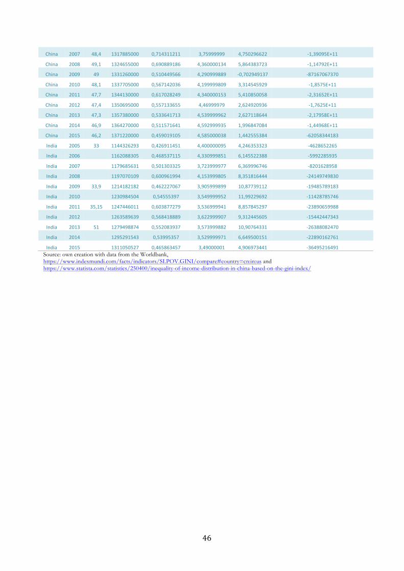
46

China 2007 48,4 1317885000 0,714311211 3,75999999 4,750296622 -1,39095E+11

China 2008 49,1 1324655000 0,690889186 4,360000134 5,864383723 -1,14792E+11

China 2009 49 1331260000 0,510449566 4,290999889 -0,702949137 -87167067370

China 2010 48,1 1337705000 0,567142036 4,199999809 3,314545929 -1,8575E+11

China 2011 47,7 1344130000 0,617028249 4,340000153 5,410850058 -2,31652E+11

China 2012 47,4 1350695000 0,557133655 4,46999979 2,624920936 -1,7625E+11

China 2013 47,3 1357380000 0,533641713 4,539999962 2,627118644 -2,17958E+11

China 2014 46,9 1364270000 0,511571641 4,592999935 1,996847084 -1,44968E+11

China 2015 46,2 1371220000 0,459019105 4,585000038 1,442555384 -62058344183

India 2005 33 1144326293 0,426911451 4,400000095 4,246353323 -4628652265

India 2006

1162088305 0,468537115 4,330999851 6,145522388 -5992285935

India 2007

1179685631 0,501303325 3,723999977 6,369996746 -8201628958

India 2008

1197070109 0,600961994 4,153999805 8,351816444 -24149749830

India 2009 33,9 1214182182 0,462227067 3,905999899 10,87739112 -19485789183

India 2010

1230984504 0,54555397 3,549999952 11,99229692 -11428785746

India 2011 35,15 1247446011 0,603877279 3,536999941 8,857845297 -23890659988

India 2012

1263589639 0,568418889 3,622999907 9,312445605 -15442447343

India 2013 51 1279498874 0,552083937 3,573999882 10,90764331 -26388082470

India 2014

1295291543 0,53995357 3,529999971 6,649500151 -22890162761

India 2015

1311050527 0,465863457 3,49000001 4,906973441 -36495216491Source: own creation with data from the Worldbank, https://www.indexmundi.com/facts/indicators/SI.POV.GINI/compare#country=cn:in:us and https://www.statista.com/statistics/250400/inequality-of-income-distribution-in-china-based-on-the-gini-index/

inequality: is it a result of globalization?

Documents